Tracing Outflowing Metals in Simulations of Dwarf and Spiral Galaxies

Charlotte R. Christensen1 , Romeel Davé2 , Alyson Brooks3 , Thomas Quinn4, and Sijing Shen51 Physics Department, Grinnell College, 1116 Eighth Avenue, Grinnell, IA 50112, USA; christenc@grinnell.edu

2 School of Physics and Astronomy, The University of Edinburgh, Royal Observatory Edinburgh, Blackford Hill, Edinburgh, EH9 3HJ, UK3 Department of Physics and Astronomy, Rutgers University, the State University of New Jersey, 136 Frelinghuysen Road, Piscataway, NJ 08854-8019, USA

4 Astronomy Department, University of Washington, 3910 15th Avenue NE, Seattle, WA 98195-0002, USA5 Institute of Theoretical Astrophysics, University of Oslo, Postboks 1029, Blindern, NO-0315 Oslo, NorwayReceived 2018 March 26; revised 2018 August 22; accepted 2018 September 14; published 2018 November 9

Abstract

We analyze the metal accumulation in dwarf and spiral galaxies by following the history of metal enrichment andoutflows in a suite of 20 high-resolution simulated galaxies. These simulations agree with the observed stellar andgas-phase mass–metallicity relation, an agreement that relies on large fractions of the produced metals escapinginto the circumgalactic media. For instance, in galaxies with Mvir∼109.5–1010 M, we find that about ∼85% ofthe available metals are outside of the galactic disk at z=0, although the fraction decreases to a little less than halfin Milky-Way-mass galaxies. In many cases, these metals are spread far beyond the virial radius. We analyze themetal deficit within the ISM and stars in the context of previous work tracking the inflow and outflow of baryons.Outflows are prevalent across the entire mass range, as is reaccretion. We find that between 40% and 80% of allmetals removed from the galactic disk are later reaccreted. The outflows themselves are metal-enriched relative tothe ISM by a factor of 0.2 dex because of the correspondence between sites of metal enrichment and outflows. As aresult, the metal mass loading factor scales as vmetals circ

0.91h µ - , a somewhat shallower scaling than the total massloading factor. We analyze the simulated galaxies within the context of analytic chemical evolution models bydetermining their net metal expulsion efficiencies, which encapsulate the rates of metal loss and reaccretion. Wediscuss these results in light of the inflow and outflow properties necessary for reproducing the mass–metallicityrelation.

Key words: galaxies: abundances – galaxies: evolution – intergalactic medium – methods: numerical

1. Introduction

Galaxies evolve through a balance between gas accretion andoutflows. Cosmological accretion of gas from the intergalacticmedia enables the continued growth of halos (Nelson et al.2013), and metal-poor cold-gas accretion has been detectedthrough absorption on the outskirts of galaxies (Kacprzak et al.2012; Bouche et al. 2013; Crighton et al. 2013). Additionally,reaccretion of previously ejected material provides continuousfuel and can easily dominate over cosmological accretion ingalaxies with halo masses >1011–1012 M(Oppenheimer et al.2010). This material exists as metal-enriched gas in thecircumgalactic media (CGM) prior to its reaccretion (Cheunget al. 2016).

Meanwhile, gas loss from galaxies is accomplished throughfeedback-driven outflows. Such outflows are ubiquitous inhigh-redshift star-forming galaxies and local starburst galaxies(e.g., Heckman et al. 1990; Pettini et al. 2001; Shapley et al.2003; Martin 2005; Weiner et al. 2009; Steidel et al. 2010;Rubin et al. 2014), and both semi-analytic models andsimulations have found them to be necessary to reproducekey observations such as the stellar mass–halo mass relation(Scannapieco et al. 2012; Stinson et al. 2012b; Henriques et al.2013; Hopkins et al. 2013; White et al. 2015). Together withaccretion, outflows set the baryonic content within the disk andregulate star formation (Davé et al. 2012; Lilly et al. 2013;Dekel & Mandelker 2014; Christensen et al. 2016).

In addition to regulating the baryonic content in galaxies,outflows are key to establishing their metal content. Forexample, comparisons of the total metals within the interstellarmedia and stellar disk to the total mass of metals producedpredict that 20%–25% of metals remain in the stars and ISM of

Milky-Way-mass galaxies (Peeples et al. 2014) and 6%remained within the stars and ISM of a dwarf galaxy (McQuinnet al. 2015). As a result, outflows are a leading candidate toregulate the metallicity within the disks of galaxies andestablish the mass–metallicity relation (MZR; e.g., Tremontiet al. 2004; Finlator & Davé 2008; Ma et al. 2016) and itssecond-parameter dependences on star formation rate and gascontent(Davé et al. 2012). The amplitude and slope of theMZR can be explained by the tendency of outflows to reducethe effective yield and by the greater efficiency of outflows inremoving material from low-mass halos in combination withtheir reduced star formation efficiency. While analytic modelscan explain the MZR by parameterizing metal inflow andoutflow efficiencies (Erb 2008; Spitoni et al. 2010; Peeples &Shankar 2011; Davé et al. 2012; Lilly et al. 2013), these modelsgenerally do not account for the reaccretion of metal-enrichedmaterial. Additionally, many of these models assume thatoutflows share the same metallicity as the ISM, whileobservations show evidence for metal enrichment comparedto the ISM (Chisholm et al. 2016). Understanding the rates ofreaccretion and the relative enrichment of outflows is key tounderstanding the source of the MZR.A corollary to the outflow-driven metal depletion of disk

material is the redistribution of metals to the CGM and beyond.Since metals originate primarily in the stellar disks of galaxies,their presence throughout the CGM provides a tracer of thehistory of inflows and outflows. In particular, strong transportof metals by galactic outflows is indicated by the large, oxygen-rich halos surrounding present-day (Prochaska et al. 2011;Tumlinson et al. 2011) and high-redshift (Lehner et al. 2014)star-forming galaxies. Observations of metal-line absorption

The Astrophysical Journal, 867:142 (19pp), 2018 November 10 https://doi.org/10.3847/1538-4357/aae374© 2018. The American Astronomical Society. All rights reserved.

1

around dwarf galaxies (Bordoloi et al. 2014), around theAndromeda galaxy (Lehner et al. 2015), and throughoutthe intergalactic medium (IGM; e.g., Cooksey et al. 2013;D’Odorico et al. 2013; Michael Shull et al. 2014) provideadditional evidence for outflow-driven enrichment. On thetheoretical side, simulations generally require strong outflowsfrom stellar feedback in order to reproduce the rapidlyadvancing observations of metal lines around galaxies (e.gStinson et al. 2012b; Ford et al. 2013; Hummels et al. 2013;Shen et al. 2013; Suresh et al. 2015). Metal-line absorptionobservations also provide a range of constraints to the thermaland dynamical states of the CGM and indicate a primarilybound, multiphase CGM with photoionized and/or collision-ally ionized gas embedded in a hotter low-density medium (fora review, see Tumlinson et al. 2017).

Galaxy-formation simulations can both provide the prove-nance of metals in the disk and halo, and establish the historyof metal accretion and outflow. Simulations thus far haveprimarily focused on examining total baryonic mass loss andreaccretion (e.g., Oppenheimer et al. 2010; Woods et al. 2014;Muratov et al. 2015; Christensen et al. 2016; Anglés-Alcázaret al. 2017). They have tended to converge on mass loadingfactors with mass scalings between those expected formomentum- and energy-conserving winds. Simulations havealso tended to agree that recycling of material is common, fuelslate-time star formation (Oppenheimer et al. 2010; Woods et al.2014), and modifies the angular momentum profile (Brooket al. 2012; Übler et al. 2014; Christensen et al. 2016).However, the fate of outflowing gas, including the rates andtimescales of outflow reaccretion, are highly model-dependent,illustrating the importance of largely unexamined processeshappening within the CGM. The examination of metals withinand surrounding galaxy halos can help delineate betweenmodels by, for instance, tracing the eventual distribution ofstellar-enriched material. As an example of this type oftheoretical investigation, Shen et al. (2012) found satelliteprogenitors and nearby dwarf galaxies to be the source of 40%of metals within 3 Rvir of a z=3 progenitor of a Milky-Way-mass halo. In a different investigation, Muratov et al. (2017)found high recycling rates of metals at early times and in low-mass galaxies, leading to similar metallicities of inflowing andoutflowing material within the central halos. In contrast,outflows from their L

*

galaxies at low redshift were veryweak, leading to the accumulation of metals within stars. Weexpand upon these types of studies by following theaccumulation of metals within galaxies by tracing gas flows.

Following on the work of Christensen et al. (2016), we use asuite of galaxy-formation simulations to quantify the cycle ofmetal production, loss, and accretion over two and a half ordersof magnitude in virial mass. By tracking the history ofsmoothed particle hydrodynamic gas particles, we identifyinstances of accretion and ejection, determine the eventuallocation of the metals produced by the galaxy, and measure themetallicity of the outflows. In Section 2, we present the suite ofsimulations and describe the analysis. Results are presented forthe redshift zero metal census (Section 3.2) and metaldistribution (Section 3.3), the history of metal cycling(Section 3.4), the metallicity of outflows (Section 3.5), andthe metal mass loading factor (Section 3.6). These results arediscussed in light of the MZR and other works (Section 4), andour conclusions are presented in Section 5.

2. Simulation and Analysis

We used cosmological simulations of seven individualvolumes to follow the history of metals in 20 field galaxieswith final virial masses between 109.5 and 1012 M (Table 1).This is the same set of simulations analyzed in Christensenet al. (2016). An overview of the sample is given below, and adescription with greater detail can be found in Brookset al. (2017).These simulations were computed using the N-body+

SPH code, GASOLINE (Wadsley et al. 2004). GASOLINE is anSPH extension to the parallel, gravity-tree-based N-body codePKDGRAV (Stadel 2001). The simulations assume a ΛCDMcosmology using WMAP3 (Spergel et al. 2007) parameters:Ω0=0.24, Λ=0.76, h=0.73, and σ8=0.77. In order toachieve high resolution while including the cosmological context,we used the “zoom-in” volume renormalization technique (Katz &White 1993). The final sample includes galaxies selected from amedium-resolution 503 Mpc3 volume and a higher resolution 253

Mpc3 volume. In the high-resolution (medium-resolution) simula-tions, the force spline softening length is ò=87 (170)pc, and theparticle masses for the dark matter, gas, and stars (at theirformation) are, respectively, 1.6 (13)×104, 3.3 (27.0)×103, and1.0 (8.0)×103Me.

GASOLINE follows non-equilibrium abundances of H (includ-ing H2) and He species. Photoionization and heating rates arebased on a redshift-dependent cosmic ultraviolet background6

while H2 dissociation is based on the Lyman–Werner radiationproduced by nearby star particles (Christensen et al. 2012). Hand He cooling channels include collisional ionization (Abelet al. 1997), H2 collisions, radiative recombination (Black 1981;Verner & Ferland 1996), photoionization, bremsstrahlung, andline cooling (Cen 1992) Metal-line cooling rates are calculatedfrom CLOUDY (version 07.02; Ferland et al. 1998) models basedon the gas temperature, density, metallicity, and cosmic UVbackground under the assumptions of ionization equilibrium andoptically thin gas.Star formation proceeds stochastically according to

pm

me1 , 1c t tgas

star

X

X XH2

H2 H I dyn*= - - D+( ) ( )

where p is the probability of a gas particle spawning a starparticle in a time step Δt, mgas is the mass of the gas particle,mstar is the mass of the potential star, c*=0.1 is the star-forming efficiency, XH2 and XH I are the mass fractions of theparticle in the form of H2 and H I, respectively, and tdyn is thedynamical time. The dependency on the H2 abundance ensuresthat star formation happens in dense (ρ10 amu cm−3), coldgas; however, star formation is technically allowed in any gasparticle with densities greater than 0.1 amu cm−3 and tempera-tures less than 103 K.Energy from Type II supernovae (SNe II) is distributed to the

surrounding gas particles according to the “blastwave” approach(Stinson et al. 2006), assuming a Kroupa et al. (1993) initialmass function (IMF) and the canonical 1051 ergs per SN. In thissubgrid recipe, the cooling of feedback-affected particles isdisabled for the theoretical lifetime of a hot, low-density shellproduced during the momentum-conserving phase of the SN

6 The cosmic ultraviolet background used is an unpublished updated versionof Haardt & Madau (1996), specified in CLOUDY (Ferland et al. 1998) as“table HM05.”

2

The Astrophysical Journal, 867:142 (19pp), 2018 November 10 Christensen et al.

remnant (McKee & Ostriker 1977). This recipe differs frommany other recipes (e.g., Springel & Hernquist 2003; Davé et al.2011; Scannapieco et al. 2012) in that no momentum kick isadded to the particles; the particle remains hydrodynamicallycoupled to the rest of the simulation, and the feedback dependsonly on the local gas properties. We do not include a separatemodel for other forms of stellar feedback, such as radiationpressure (e.g., Stinson et al. 2012a; Hopkins et al. 2013), thathelp drive a galactic wind through additional momentum transferor by making the gas more responsive to the SN feedback.Instead, this blastwave recipe represents the total stellar feedbackfrom young stars.

We follow the production and distribution of oxygen andiron separately. Metals are returned to the ISM both throughSNe I and II and stellar winds. For SNe II, metals aredistributed to the same gas particles as the feedback energy,assuming the production rates from Raiteri et al. (1996) withyields from Woosley & Weaver (1995). SNe Ia are calculatedto occur using the rates from Raiteri et al. (1996). Each SN Iaproduces 0.63 M iron and 0.13 M oxygen (Thielemann et al.1986), which are transferred to the nearest gas particles. Energyfrom SNe Ia is also distributed to the gas particles within thesmoothing kernel; however, cooling is not disabled for theseparticles as it is for SNe II. Mass is returned to the ISM bystellar winds using mass loss rates from Weidemann (1987).This mass is distributed to gas particles within the smoothing

sphere of the star particle, assuming the same metallicity as thestar particle.Metals are further distributed throughout the gas through

diffusion (Shen et al. 2010). In this model, based onSmagorinsky (1963), subgrid turbulent mixing is treated as ashear-dependent diffusion term. As a result, the highestdiffusion rates are calculated for shearing flows. Instances ofcompressive or purely rotating flows result in no diffusion. Atunable parameter, called the metal diffusion coefficient, is usedto scale the strength of diffusion. For these simulations, aconservative value of 0.01 was chosen for the metal diffusioncoefficient.

2.1. Postprocessing Analysis

Individual halos were selected from snapshots of thesimulations during postprocessing. We used AMIGA’S HALOFINDER (Gill et al. 2004; Knollmann & Knebe 2009),7 in whichareas of overdensity are identified using grid hierarchy and thengravitationally unbound particles are iteratively removed fromthe prospective halos. The virial radius, Rvir, is defined suchthat the average halo density is a multiple of the backgrounddensity. This multiple evolves with redshift but is approxi-mately equal to 100 times the critical density at z=0. The

Table 1Properties of the Set of Galaxies at z=0

Sim. Softening Gas Particle Halo ID Virial Mass Gas Mass Stellar Vf

Name Length Mass in Rvir Mass(pc) (M) (M) (M) (M) (km s−1)

(1) (2) (3) (4) (5) (6) (7)

h799 87 3.3×103 1a,b,c 2.4×1010 1.4×109 1.4×108 554 6.8×109 4.1×107 1.8×107 336 4.4×109 3.9×107 3.5×106 27

h516 87 3.3×103 1a,b,c,d 3.8×1010 2.3×109 2.5×108 672 1.5×1010 3.7×108 8.1×107 34

h986 170 2.7×104 1b,c 1.9×1011 1.7×1010 4.5×109 1032 5.9×1010 3.2×109 1.2×109 773 3.8×1010 2.4×109 4.6×108 768 1.1×1010 6.4×107 4.0×107 3515 4.4×109 8.7×107 6.2×106 2916 3.2×109 3.0×107 2.3×106 27

h603 170 2.7×104 1b,c 3.4×1011 3.1×1010 7.8×109 11523 1.0×1011 6.1×109 3.8×109 753 2.9×1010 1.8×108 3.9×108 50

h258 170 2.7×104 1b,e 7.7×1011 5.6×1010 4.5×1010 1824 1.1×1010 1.4×108 5.9×107 43

h285 170 2.7×104 1b 8.8×1011 6.3×1010 4.6×1010 1644 3.4×1010 1.2×109 3.9×108 649 1.2×1010 3.1×108 5.4×107 52

h239 170 2.7×104 1b 9.1×1011 8.1×1010 4.5×1010 165

Notes.a Appears in Governato et al. (2012).b Appears in Munshi et al. (2013).c Appears in Christensen et al. (2014).d Appears in Christensen et al. (2012).e Appears in Zolotov et al. (2012).

7AMIGA’S HALO FINDER is available for download athttp://popia.ft.uam.

es/AHF/Download.html.

3

The Astrophysical Journal, 867:142 (19pp), 2018 November 10 Christensen et al.

main progenitor of each galaxy was traced back in time fromredshift zero through the creation of a merger tree and wasdefined at each snapshot to be the halo that contained themajority of particles from the subsequent snapshot.

2.1.1. Inflow/Outflow Identification

After the main progenitor halo had been identified at eachsnapshot, we identified all instances of accretion and outflow.To do this, gas particles were classified in each snapshot asbeing part of the disk, within the halo, and outside the galaxy.Accretion events and ejection were found by identifying theinstances when particles moved from one classification toanother. The time resolution of this tracking comes from thespacings between snapshots, which were ∼100 Myr for all ofthe simulations. As a result, we were unable to measureaccretion and ejection at a time resolution less that 100Myr,and it is possible for accretion and ejection events to have beenmissed if a particle left and reentered the galaxy between timesteps.

We used the following criteria for classifying particles intodifferent components. Gas particles are defined as being in thehalo if they are within the virial radius. They are defined aswithin the disk if they (1) have density >0.1 amu cm−3, (2)have temperature <1.2×104 K, and (3) are less than 3 kpcfrom the plane of the disk. These disk parameters were chosento thermodynamically select for the ISM and to spatiallyeliminate cool gas in accreting satellites.

Particles are classified as being accreted onto the halo eachsnapshot they go from not being part of a halo to beingincluded in it. Similarly, particles are classified as beingaccreted onto the disk each step they are included in the diskafter not having been included in it during the previoussnapshot. Particles may, therefore, be accreted onto the diskor halo multiple times. As may be expected, particles areidentified as leaving the disk each time they move from disk tohalo. However, we also further divided the ejected materialbetween material that is merely heated and material that passesmore stringent constraints for ejecta. This division is necessaryas it is common for gas particles to be heated by SNe totemperatures greater than 1.2×104 K but then to quicklyradiate their energy away without having a substantial effect onthe disk dynamics. Therefore, we defined the followingclassifications, with each later classification a subset of theprevious ones.

1. Material removed from the disk includes all gas that isclassified as disk material in one step and outside of thedisk in the next step.

2. Material ejected from the disk includes those particlesremoved from the disk that become dynamically unboundfrom the baryonic disk. Specifically, a particle is definedto be “unbound from the disk” at any snapshot afterleaving a disk if its velocity exceeds the escape velocityfor a mass equal to the sum of the ISM and stellar masslocated at the center of the galaxy. This classification ismost similar to what is generally referred to as outflows.

3. Material expelled from the halo includes all particles thatare classified as being in the disk in one instance and atany later point travel beyond the virial radius. Note thatwe are focusing our analysis on gas that was ever part ofthe ISM and so do not include in our analysis gas that wasonly ever part of the halo prior to leaving it.

Together, these classifications allowed us to determine all gasparticles that were ever part of the halo or disk and their historyof accretion and outflow.One additional complication in tracking the flow of metals in

and out of galaxies is that metal diffusion is included in thesimulation. As a result, metals may pass from within the disk tothe halo through diffusion, as opposed to an SPH particleleaving the disk. Therefore, it is best in these circumstances tothink of the SPH particles as tracer particles of the metaldistribution that pick up on bulk motion while missing some ofthe small-scale diffusion. Based on comparing the mass ofmetals within the disk and halo at each time step to thatexpected from particle tracing, we were able to account for90% of the metal movement from disk to halo and back.Throughout this paper, we note those aspects of the analysiswhere diffusion could further affect the results and specify howwe addressed it.

3. Results

3.1. Mass–Metallicity Relation

We assess our simulated galaxies with reference to theobserved MZR. These simulations were previously shown to beconsistent with the redshift zero gas-phase MZR, stellar mass–halo mass relation, and the baryonic and i-band Tully–Fisherrelation (Christensen et al. 2016). Galaxies generated with aprevious version of GASOLINE have also been shown todemonstrate an evolving gas-phase MZR (Brooks et al. 2007).Here, we expand our analysis to show our simulated galaxiesalong the gas-phase MZR at multiple redshifts and the redshiftzero stellar MZR.Figure 1 compares the gas-phase oxygen abundances

at z=3, 2.3, 0.8, and 0 to the observed values. In orderto best mimic observations, stellar masses are determinedfrom broadband magnitudes using KCORRECT (Blanton &Roweis 2007). Metallicities were calculated using the starformation rate-weighted average gas particle oxygen abun-dances. Weighting by the star formation rate (i.e., theprobability of the gas particle forming a star) was chosen tomimic the measurement of metallicities in star-forming regionsof observed galaxies. The simulated galaxies show a slightincrease in the normalization of the MZR with decreasingredshift.We compare our simulated galaxies to observational data

from z∼3 (Mannucci et al. 2009), z∼2.3 (Erb et al. 2006;Steidel et al. 2014; Sanders et al. 2015), z∼0.8 (Zahid et al.2011), and z∼0 (Tremonti et al. 2004; Lee et al. 2006;Andrews & Martini 2013). These observations were madebased on different diagnostics using different calibrations, andthe systematic uncertainty between the different metallicitydiagnostics could be as much as 0.7 dex (Kewley & Ellison2008). In order to demonstrate the evolution of the MZR, weshowed or converted to the N2 calibration (Pettini & Pagel2004) where possible; in particular, we used the formula inKewley & Ellison (2008) to transform Tremonti et al. (2004)and Zahid et al. (2011) to the N2 calibration. Compared toobservations, the simulations at z=3 may have slightly toohigh of metallicities. However, given the lack of overlap in themass range and the large systematic uncertainties in theobserved metallicities, the simulations appear largely consistentwith observations.

4

The Astrophysical Journal, 867:142 (19pp), 2018 November 10 Christensen et al.

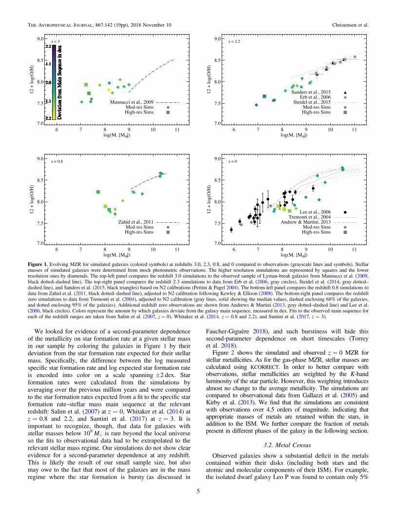
We looked for evidence of a second-parameter dependenceof the metallicity on star formation rate at a given stellar massin our sample by coloring the galaxies in Figure 1 by theirdeviation from the star formation rate expected for their stellarmass. Specifically, the difference between the log measuredspecific star formation rate and log expected star formation rateis encoded into color on a scale spanning±2 dex. Starformation rates were calculated from the simulations byaveraging over the previous million years and were comparedto the star formation rates expected from a fit to the specific starformation rate–stellar mass main sequence at the relevantredshift: Salim et al. (2007) at z=0, Whitaker et al. (2014) atz=0.8 and 2.2, and Santini et al. (2017) at z=3. It isimportant to recognize, though, that data for galaxies withstellar masses below 109 M is rare beyond the local universeso the fits to observational data had to be extrapolated to therelevant stellar mass regime. Our simulations do not show clearevidence for a second-parameter dependence at any redshift.This is likely the result of our small sample size, but alsomay owe to the fact that most of the galaxies are in the massregime where the star formation is bursty(as discussed in

Faucher-Giguère 2018), and such burstiness will hide thissecond-parameter dependence on short timescales (Torreyet al. 2018).Figure 2 shows the simulated and observed z=0 MZR for

stellar metallicities. As for the gas-phase MZR, stellar masses arecalculated using KCORRECT. In order to better compare withobservations, stellar metallicities are weighted by the K-bandluminosity of the star particle. However, this weighting introducesalmost no change to the average metallicity. The simulations arecompared to observational data from Gallazzi et al. (2005) andKirby et al. (2013). We find that the simulations are consistentwith observations over 4.5 orders of magnitude, indicating thatappropriate masses of metals are retained within the stars, inaddition to the ISM. We further compare the fraction of metalspresent in different phases of the galaxy in the following section.

3.2. Metal Census

Observed galaxies show a substantial deficit in the metalscontained within their disks (including both stars and theatomic and molecular components of their ISM). For example,the isolated dwarf galaxy Leo P was found to contain only 5%

Figure 1. Evolving MZR for simulated galaxies (colored symbols) at redshifts 3.0, 2.3, 0.8, and 0 compared to observations (grayscale lines and symbols). Stellarmasses of simulated galaxies were determined from mock photometric observations. The higher resolution simulations are represented by squares and the lowerresolution ones by diamonds. The top-left panel compares the redshift 3.0 simulations to the observed sample of Lyman-break galaxies from Mannucci et al. (2009,black dotted–dashed line). The top-right panel compares the redshift 2.3 simulations to data from Erb et al. (2006, gray circles), Steidel et al. (2014, gray dotted–dashed line), and Sanders et al. (2015, black triangles) based on N2 calibrations (Pettini & Pagel 2004). The bottom-left panel compares the redshift 0.8 simulations todata from Zahid et al. (2011, black dotted–dashed line), adjusted to N2 calibration following Kewley & Ellison (2008). The bottom-right panel compares the redshiftzero simulations to data from Tremonti et al. (2004), adjusted to N2 calibration (gray lines, solid showing the median values, dashed enclosing 68% of the galaxies,and dotted enclosing 95% of the galaxies). Additional redshift zero observations are shown from Andrews & Martini (2013, gray dotted–dashed line) and Lee et al.(2006, black circles). Colors represent the amount by which galaxies deviate from the galaxy main sequence, measured in dex. Fits to the observed main sequence foreach of the redshift ranges are taken from Salim et al. (2007, z = 0), Whitaker et al. (2014, z=0.8 and 2.2), and Santini et al. (2017, z=3).

5

The Astrophysical Journal, 867:142 (19pp), 2018 November 10 Christensen et al.

of all the metals produced by its stars in its disk (1% in the formof stars; McQuinn et al. 2015). On the more massive side,Peeples et al. (2014) found that in galaxies with stellar massesbetween 109.2 M and 1011.6 M, approximately 20%–25%(with an uncertainty range between 10% and 40%) of themetals produced by the stars remained in the disks of thegalaxies. This metal deficit is a companion to the “MissingBaryon Problem”; like the missing baryons, these metals arepresumed to largely be contained within the CGM. Here weexamine the metal census for our population of galaxies. Sincewe have excluded satellites (as defined by Amiga Halo Finder)from our sample, our analysis focuses on metals lost forreasons other than stripping by a more massive halo.

Figure 3 shows the fraction of metals available to eachgalaxy contained within the halo (r<Rvir), the stars, and theISM at redshifts two and zero. The mass of metals available isdefined to be the sum of all metals produced by the stars withinthe final halo. To do this, we used the same metal productionmodels included within GASOLINE for SNe II and SNe Ia tocalculate the mass of oxygen and iron produced by all starparticles given their age and metallicity and assuming a Kroupaet al. (1993) IMF. Since observations do not tally the metalscontained within stellar remnants, we also did not include themwhen calculating the mass of metals contained within the stars.Specifically, we reduced the mass of metals in each star particleby the mass fraction of that particle in the form of stellarremnants based on its age and metallicity.

We find that a substantial fraction of metals are lost fromgalaxies of all masses; by z=0 between 35% and 85% of themetals had been removed from the galactic disk and between15% and 75% from the entire halo, as defined by the virialradius. The metal fractions contained in stars show a strongmass dependency with higher mass galaxies retaining a greaterfraction of metals in stars. By z=0, the fraction of metalscontained within the entire halo also shows some evidence formass scaling for those halos with M*>107 M. Within thismass range, lower mass galaxies appear more able to remove

metals through outflows, likely because of their lowergravitational potential. This result mirrors a similar one inChristensen et al. (2016), where 20% of baryons ever accretedto the galaxy were retained within it at z=0 for dwarfgalaxies, while closer to 80% were retained within Milky-Way-mass galaxies. However, the three galaxies with z=0 stellarmasses <107 M complicate this mass trend by retainingrelatively large fractions of their metals within Rvir. Thesegalaxies may illustrate a transition to a mass range where thelow gravitational potentials that could aid metal loss arecounterbalanced by incredibly low rates of star formation.Notably, similar fractions of metals are retained within the ISMfor galaxies of all masses. Similarly, the fraction of metalsretained within the CGM does not show a clear mass trend.The metal deficit is well established even by z=2, with

generally ∼60% or less of metals retained within the virialradius. This result is consistent with observations indicatingthat the missing metals problem is already in place by z∼2(e.g., Pagel 1999). In the evolution from z=2 to z=0, thefraction of metals retained within the lowest mass galaxies(M*<107.5) is reduced as outflows continue to expel metals.

Figure 2. Stellar MZR for simulated galaxies (colored symbols) compared toobserved values (grayscale symbols). Redshift zero stellar metallicities fromsimulations were calculated using the K-band weighted average metallicity ofall star particles in the galaxy. Stellar masses of simulated galaxies weredetermined from mock photometric observations. The higher resolutionsimulations are represented by teal filled squares and the lower resolutionones by diamonds. Gray filled circles represent observational data for dwarfirregular and dwarf spheroidal galaxies from Kirby et al. (2013). Black linesshow observational data from Gallazzi et al. (2005); the solid line shows themedian values, and the dotted lines show the 16th and 84th percentile data. Thesimulated galaxies appear consistent with the observed data, and there is nodistinction between the two different resolutions.

Figure 3. Redshift z=2 and z=0 location of all the metals produced by eachof the galaxies. The metal mass contained in each component is normalized byMz,available, which is defined to be the sum of all metals produced by the starswithin the final halo. Each bar represents a unique galaxy with the fractioncontained within stars shown in green, the fraction contained within the ISMshown in maroon, and the fraction within the virial radius but not within theISM and stars (i.e., the CGM) shown in blue. In part because of their largerstellar mass, more massive galaxies retain a greater fraction of their metals instars. The metal fraction retained within the CGM does not show a clear masstrend and, by z=0, neither does the fraction retained within the ISM.

6

The Astrophysical Journal, 867:142 (19pp), 2018 November 10 Christensen et al.

By contrast, the metal mass fraction within the highest massgalaxies increases, primarily as those metals become lockedinto stars. Across the entire range of galaxies, the fraction ofmetals within the halo gas tends to decrease over time.

A similar analysis of numerical simulations in Muratov et al.(2017) found comparable z=0 mass trends in metal mass loss.As in ours, they found that greater fractions of the availablemetals were locked within stars for Milky-Way-mass galaxiesthan for dwarf galaxies, while the fraction retained within theISM showed a negligible mass trend. However, higher amountsof metals were retained in the CGM, stars, and ISM in theirsimulations than in ours. The difference was greatest in theMilky-Way-mass galaxies (M*∼4×1010 M). While wefind that 50%–60% of available metals are retained in stars and80%–90% within a virial radius at a redshift of zero, they foundcloser to 80% in stars and >90% within a virial radius.Differences between these results are most likely due todifferences in implementing feedback, as will be discussedfurther in Section 4.

Observational constraints for halos in this mass range arelimited. Nevertheless, we draw some comparisons at both thehigh and the low ends. The largest survey of the fraction ofmetals retained in stars within dwarf galaxies are for eightdwarf spheroidal Milky Way satellites with stellar massesbetween 5.6×105 and 1.8×107 M Kirby et al. (2011). Theydetermined that <1%–4% of the metals produced by the starsin their sample of galaxies were retained within the stellarcomponent (with the greatest fraction retained in the mostmassive dwarf), which they found suggestive of an energy-driven scaling for the mass loading factor. In comparison, wefound that our four galaxies in this mass range retained asimilar fraction of their metals in stars (specifically, 3%, 4%,4%, and 6% for the galaxies with masses between 2.3×106

and 1.8×107 M). Likewise, these simulations exhibit massloading factors with energy-driven scalings (Christensenet al. 2016). Despite this apparent agreement, it is dangerousto draw strong conclusions from this comparison, as theobserved sample of dwarf spheroidal galaxies has a substan-tially different environment and evolutionary history than ourfield dwarf irregular galaxies. In particular, tidal and/or rampressure stripping acting on the observed satellites may haveimpacted the fraction of metals retained within stars bycontributing to metal loss prior to the cessation of starformation. Furthermore, we cannot compare the fraction ofmetals retained within the ISM for our sample to data fromKirby et al. (2011), as dwarf spheroidal galaxies are necessarilylacking an ISM because of their satellite environment.

Observational measurements of the metal census for fielddwarf galaxies are difficult to achieve because H II regions arerequired in addition to stellar spectroscopy. The only currentlyavailable observational metal census for a field dwarf galaxy isfor Leo P (McQuinn et al. 2015). Leo P shows no evidence ofinteraction and has a metallicity consistent with a low-luminosity extension of the MZR, implying that it is arepresentative galaxy. It has a stellar mass half that of ourlowest mass galaxy and has a similar, although slightly smaller,metal fraction retained within its stars as our two lowest massgalaxies (3% and 4% for the simulated dwarf galaxies and∼1% in Leo P; McQuinn et al. 2015). When comparingthe fraction of metals retained within the ISM, it is important touse similar definitions in selecting ISM material. In Figure 3,we use the same definition of “disk” material as in our particle

tracing code: (1) density >0.1 amu cm−3, (2) temperature<1.2×104 K, and (3) less than 3 kpc from the plane of thedisk (Section 2.1.1). However, observations generally (and inthe case of Leo P, specifically) measure ISM mass through H Iand, when detectable, H2. In low-mass halos, in particular, thedifference between these two ISM definitions can besignificant. Therefore, we also calculate the fraction of metalsretained within the ISM as determined by scaling gas particleswithin 3 kpc of the disk plane by their HI and H2 content. Wecalculate that our two lowest mass galaxies retained 9% and10% of their metals within the ISM defined this way, comparedto the ∼4% determined for Leo P. This factor of 2 differencemay imply that the simulations retain too many of their metalsin their ISM. Or it is possible that the discrepancy can beexplained by the differences in stellar masses between Leo Pand the simulations, and the stochasticity in metal retentionamong dwarf galaxies. Larger samples of both observed andsimulated dwarf galaxies will be needed to draw firmerconclusions as to the consistency of the results.For our most massive galaxies, the metals retained can be

compared with observations from Peeples et al. (2014). Theaverage 64% of metals we found retained in Milky-Way-massgalaxy disks is substantially greater than the ∼25% measuredby Peeples et al. (2014). This is a qualitatively similar butsmaller level of disagreement than Muratov et al. (2017) hadwith Peeples et al. (2014). It is possible that this discrepancycould argue for the need for an additional form of feedback,such as AGN feedback, in the most massive of our galaxies.However, comparisons to the gas and stellar MZR confirm thatthe metallicities in our simulations are consistent with observedvalues (Section 3.1). Given that the metal content within theISM and stars agrees with observations, the discrepancy withPeeples et al. (2014) almost certainly originates fromdifferences in how the available metal mass is calculated.While GASOLINE uses the yields from Woosley & Weaver(1995) for SNe II, Peeples et al. (2014) assumed higher yieldsbased on other models. Additionally, Peeples et al. (2014)assumed significantly higher mass loss rates (∼55%) fromsimple stellar populations using a Chabrier (2003) IMF thanGASOLINE does using a Kroupa et al. (1993) IMF. As a result,Peeples et al. (2014) calculated about four times as much metalmass available for the same stellar mass as our simulationsproduce. Assuming a higher value of Mz,available than what isactually used in the simulations profoundly reduces thepresumed fraction of metals retained in both the disk and theCGM (defined to be material within 150 kpc of the galaxy inPeeples et al. 2014).By changing our calculation of the metals available (and, to a

much lesser extent, how we select for ISM and CGM material)to be consistent with Peeples et al. (2014), we can compareMilky-Way-mass galaxies ( M Mlog 10.6* ~( ) ) and slightlylower mass spiral galaxies (9.5<log(M*/M)<10.0) tomeasurements from Peeples et al. (2014). Specifically, underthese assumptions, the simulated Milky-Way-mass galaxies arepredicted retain on average 13% of their metals in their diskand 17% within 150 kpc, compared to the observed ∼25% and>30% for those components. Similarly, the simulated lowermass spiral galaxies would be predicted to retain on average8% in their disk and 15% within 150 kpc, compared to theobserved ∼20% and >40%. So, by changing the calculation ofMz,available to follow the method in Peeples et al. (2014), wemoved from predicting about twice as many metals retained in

7

The Astrophysical Journal, 867:142 (19pp), 2018 November 10 Christensen et al.

the CGM and disks of spiral galaxies to half as many.Therefore, we cannot yet claim agreement with Peeples et al.(2014), but uncertainties in metal yields also limit the ability ofobservations to constrain the simulations.

3.3. Redshift Zero Distribution of Metals

Observations of the CGM have shown metals distributed outto the virial radius (e.g., Tumlinson et al. 2011), and in somecases, O VI has been observed out to R5 vir (Pratt et al. 2018),demonstrating the far reach of outflows. Simulations have alsohighlighted the reach of outflows, especially in low-massgalaxies. Ma et al. (2016) found that their dwarf galaxiesretained only 2%–20% of their metals within a virial radius,while Shen et al. (2014) calculated that 87% of the metalsproduced by a group of seven dwarf galaxies were spread overa 33 Mpc3 volume, equating to a distance of ∼17.5 Rvir of themost massive dwarf galaxy. Here, we examine the extent ofmetal enrichment of the CGM by showing the metal fractioncontained within a given radius. In Figure 4, the left-handpanels shows the normalized cumulative histogram of thez=0 locations of gas or stars ever part of the galaxy halo sincethe start of the simulation. The right-hand panels weight thoseparticles by their metal content to demonstrate the eventualdistribution of metals. The top panels show the physicaldistribution of the matter, while the bottom panels show thedistances scaled by the virial radius. All histograms are shownout to 300 kpc. This distance corresponds to the largest impactparameter typically used for observations of the CGM andensures that the analysis is within the highest resolved regionsof the simulation. Note that the normalization factor for this

plot differs from the mass of metals available used inSection 3.2, as in this plot only those metals contained withingas or star particles that were ever part of the main progenitorare considered.Since metal diffusion can occur across gas particles, it is

possible that the eventual location of some metals may not bethe same as the gas particle they exited the halo with. Moreexactly, one may consider the gas particles to be tracer particlesassociated with the underlying metal distribution. Therefore,the eventual location of the gas particles follows the bulkmotion of the metals at a limited resolution. In order to avoidunderestimating the mass of metals exiting the virial radiusbecause of metal diffusion we make the following adjustmentwhen generating Figure 4. For those particles that exit the virialradius, we consider their metallicity at the time they exit, whilein all other instances the redshift zero metallicity is used.As would be expected from the substantial fractions of

metals beyond the virial radius (Figure 3), the metal enrichmentcontinues far beyond Rvir. The distribution of both total massand metals relative to the virial radii shows clear trends withgalaxy mass. Metals and total mass tend to remain closer to thecenters of more massive galaxies because of their largergravitational potential. However, this mass trend is complicatedby the three lowest mass galaxies, whose metals are lessdispersed than most of the medium-mass galaxies. The lack ofmass and metal dispersal in these smallest galaxies likelyresults from their extremely low star formation rates.We find that on average about 78% of metals are contained

within the virial radii of the three most massive halos. Galaxieswith virial masses between 109.5 and 1010.5 M only retain onaverage 45% percent of their metals within a virial radius. In

Figure 4. Normalized, cumulative histograms of the z=0 location of the mass (left) and metals (right) ever within the galaxy halo since z=3 as a function of radius.The top panels show the absolute distances, while in the bottom panels the distances are scaled by the virial radius of the corresponding galaxy. The line colors,spanning from yellow (low mass) to purple (high mass), represent the galaxy mass. The shape of the curves and the relationship between different galaxies are similarfor the mass and metal histograms. However, the metal mass fraction tends to be higher at small radii and flatten off more slowly at large radii.

8

The Astrophysical Journal, 867:142 (19pp), 2018 November 10 Christensen et al.

general, the trend of increasing dispersal relative to the virialradius with decreasing virial mass is similar to that found byMa et al. (2016), although these simulations have slightly moremetals retained within a virial radius for dwarfs and slightlyfewer for Milky-Way-mass galaxies than in Ma et al. (2016).For instance, in Ma et al. (2016), essentially all metalsproduced by their Milky-Way-mass galaxy were retainedwithin one virial radius (and almost all within 0.1 Rvir) whiletheir Mvir=2.5×109 M galaxy retained only 2% of itsmetals within a virial radius.

Metals are generally more likely to be retained close to thecenter of the galaxy than total mass. This phenomenon isapparent in the shallowness of the histograms of cumulativemetals at very small radii. It can be seen even more clearlythrough the average metallicity of the particles—i.e., the ratioof the histogram of metals to the histogram of the mass that wasever within the galaxy disk (Figure 5). For almost all of thegalaxies, the metallicity is relatively high at the center anddrops toward the virial radius. This relatively high metalretention can be explained by the tendency of star formation tooccur throughout the galactic disk, where the gas iscomparatively metal-enriched, resulting in metals becominglocked into stars. After the virial radius, the metallicities tend torise again. The change from inside to outside of the virial radiusis a result of our selection—since only those particles that wereonce within the virial radius are analyzed, those particles thatare outside of the virial radius at z=0 are especially likely tohave been part of an outflow. The frequent continued rise inmetallicity after Rvir results from the correlation between metalinjection and SN energy. Those particles that travel fardistances most likely received large amounts of both energyand metals.

3.4. History of Metal Enrichment

The history of metal enrichment of both the CGM and ISMcan be seen by chronicling pristine accretion, star formation,outflows, and reaccretion. At any point in time, the metal

content within the ISM and stars is the sum of the metalsaccreted from outside the halo (either in the form of gas orstars) and the metals produced by the stars within the galaxyminus the net metal loss in outflows. This net metal loss is thetotal mass of metals that have left the galaxy minus the mass ofmetals that reaccreted onto it. In Figure 6, we show the historyof these processes and the total metal mass contained within theISM and stars as a function of time for each of the simulatedgalaxies.Metal production within the galaxy by stars is shown by the

long-dashed green line. Similar to the amount of “metalsavailable” generated for Figure 3, the metal production rates arecalculated using the same enrichment models as GASOLINE.However, to find the metal production history, we onlyconsider the metals produced within the main progenitor. Todo this, the mass of metals produced between two snapshotswas calculated for those star particles within the mainprogenitor during the latter snapshot. Additional metals aregained through externally accreted gas and stars, frequently aspart of a merger. Rates of externally accreted metals weretallied using all gas and star particles that had previously beenexternal to the main progenitor. Gas particles and stars wereconsidered accreted at the time they first entered the galacticdisk; however, we determined the metal mass accreted usingthe metallicity of the gas particles at the time they enter thehalo. The metallicity at this earlier time was chosen to ensurethat any additional metals picked up as the particle traveledthrough the halo were not included as external accretion. For allhalos, the metals produced by a galaxy overwhelm the metalsgained through external accretion, a point that will be furtherquantified later in this section.Except in the highest mass galaxies, the mass of metals

contained in the ISM and stars is only a small fraction of thetotal metals produced and accreted from external sources, asalso seen in Section 3.2. Therefore, it is clear that metalremoval via outflows must be instrumental in setting the metalcontent of the galaxies. The cumulative mass of metalsremoved from the disk is shown as the negatively valued goldline. The subset of metals removed that achieve sufficientenergy to exceed the escape velocity of the disk, what isgenerally considered part of an outflow and what we term as“ejected,” are shown as the negatively valued red line. An evensmaller subset of metals is fully “expelled” from the halo, i.e.,they reach a distance farther than the virial radius. Thecumulative history of these metals is shown as the blue line.The fraction of metals removed from the disk that satisfy eitherthe ejected or expelled criteria depends strongly on halo mass.The more massive the halo, the higher the energy thresholds forejection and expulsion, and the less likely a particle achieving atemperature or density sufficient to not be considered removedfrom the ISM will actually be part of an outflow. An additionaldistinction between the material removed from the ISM and thesubset that is ejected or expelled can be seen in the differentshapes of the curves. The mass of metals expelled and ejectedtrack the mass of metals produced since both follow the starformation history (and, therefore, the history of stellarfeedback) in the galaxy. In contrast, the mass of metals lostfrom the disk continues to rise steeply over time as metalscontinuously rapidly pass in and out of the disk.Substantial amounts of metal mass are returned to the disk,

indicating the importance of gas recycling. We show thecumulative history of all metals reaccreted after leaving the

Figure 5. Metallicity of the material ever once within Rvir, calculated from theratio of the histogram of metals to the histogram of the mass. The spatialdistributions are scaled by the virial radius of each of the galaxies. As inFigure 4, the line colors, spanning from yellow (low mass) to purple (highmass), represent galaxy mass. Metallicities generally decrease out to Rvir. Onlythose particles ever within Rvir are included in this analysis, so particles beyondRvir at z=0 were likely once part of an outflow. This selection explains thefrequent rise in metallicity beyond Rvir.

9

The Astrophysical Journal, 867:142 (19pp), 2018 November 10 Christensen et al.

Figure 6. History of the metal buildup within galaxies. All values are scaled by the total mass of metals produced by the stars in the main progenitor by z=0. Thez=0 virial mass of each galaxy is listed in the upper-left corner of each panel. The black solid line represents the metal mass contained within the ISM and stars. Allother positive-valued lines show the cumulative histograms of the mass of metals produced by stars (green long-dashed line), accreted externally (purple dotted–dashed), reaccreted to the disk after being removed from it (gold), and reaccreted to the disk after being ejected (maroon). The solid negatively valued lines show thecumulative histograms of the mass of metals removed from the disk (gold), ejected from the disk (maroon), and expelled beyond the virial radius (light blue).Additionally, the net metal mass removed from the disk is shown by the dashed gold line. The net metal mass removed was calculated by subtracting the reaccretedmetal mass from the removed metal mass.

10

The Astrophysical Journal, 867:142 (19pp), 2018 November 10 Christensen et al.

disk (calculated by subtracting the externally accreted metalmass from the total accretion) as the positively valued goldline. For illustrative purposes, we also show the cumulativehistory of metals reaccreted as part of particles previouslyejected from the disk (red positively valued line). However, thisquantity carries the caveat that additional metals may bereaccreted after being ejected by diffusing to other accretedparticles. Therefore, this line is a lower limit on the mass ofmetals actually reaccreted following an outflow. Finally, weshow the net mass of metals removed from the disk (cumulativehistory of metals removed minus the cumulative history ofmetals reaccreted after removal) as the dashed gold line.

Reaccretion is common across our entire sample. In fact, forall galaxies, there is as much metal reaccretion after removal asthere is metal production; for the most massive galaxies,multiple cyclings of gas lead the metal reaccretion mass toexceed the metal production by factors of a few. More massivegalaxies tend to have slightly higher rates of reaccretion ofremoved metals, as shown by the difference between the totalmass of metals removed and the net mass of metals removed.Despite the prevalence of recycling, however, much of themetal mass produced remains within the CGM. In fact, the netmetal loss exceeds the total metals contained in the disk at allredshifts for any but the three most massive galaxies. Whilesome of these “permanently removed” metals escape the halo,they may also remain within Rvir, as seen when the net metalloss exceeds the mass of metals expelled (in other cases wheremergers result in the reaccretion of gas from outside the virialradius, the net metal loss from the disk may be less than thetotal mass of metals expelled).

In the remainder of this section, we further quantify how theamount of material accreted, outflowing, and reaccreted scaleswith the halo mass. To begin, we quantify the role of externalaccretion in contributing metals. The fraction of metals thatwere originally accreted from external sources as gas is shownas a function of halo mass in Figure 7. In this analysis, the massof metals accreted as gas is compared to the total mass ofmetals accreted as gas and produced within the main progenitorby z=0. As also seen in Figure 6, the fraction of metalsexternally accreted is uniformly small. However, there appearsto be a mass trend, with the most massive galaxies generally

accreting a larger fraction of their metals from external sources,probably primarily through mergers.Figure 8 shows the mass of metals in outflows divided by the

total mass of metals available (metals either produced by starsor externally accreted as gas). Because the same metals can exitthe disk multiple times, this number is frequently greater thanone. In particular, the large amount of metals removed fromthe disk compared to the amount available highlights theprevalence of both gas removal and gas reaccretion. Thelikelihood of metals being removed from the disk is largelyindependent of halo mass, because the possibility of gas beingheated is basically independent of the galaxy dynamics. Thelikelihood of metals being ejected (i.e., part of an outflow),though, is sensitive to mass, because the particles must exceedan energy threshold. As a result, in more massive galaxies, asmaller fraction of either the metals available or the metalsremoved from the disk is actually considered ejected. Even inthe most massive halos, though, ∼20% of the available metalsare ejected from the main progenitor. When considering thefraction of metals expelled beyond the virial radius for galaxieswith virial masses greater than ∼2.5×1010 M, we see asimilar, although slightly reduced, trend as for the mass ofmetals removed from the disk. Specifically, the fractionexpelled is ∝ log(Mvir/M)

−0.31 while the fraction ejectedis ∝ log(Mvir M)

−0.44. As seen in Figure 6, in these moremassive galaxies, a majority of the gas particles that exitthe disk also exit the virial radius, explaining the similarity inthe trends. For galaxies with Mvir3×1010 M, however,the fraction of metals that are expelled beyond the virial radiusis roughly constant, even as the fraction that exits the diskincreases with decreasing halo mass. As a result, in the lowestmass galaxies, a minority of the metals ejected from the diskare able to escape the virial radius. This effect is especiallystrong for the three lowest mass galaxies, which have beenpreviously shown to retain metals relatively close to theircenters (Figures 3 and 4).Figure 9 quantifies the fraction of gas reaccreted. Through-

out this section, we divide among gas removed from the disk,ejected from the disk, and expelled beyond the virial radius.The fractions of the gas that are reaccreted by z=2 andz=0 are shown as a function of halo mass. All reaccretionrates rose from z=2 to z=0 as the greater time elapsed

Figure 7. Fraction of metals within Rvir at z=0 accreted externally as gas. Thedenominator includes the sum of all metals produced and all metals accreted asgas from external sources, including through galaxy mergers. In general, alarger fraction of the metals available to higher mass galaxies are accretedexternally but the fraction of metals externally accreted is low across the entiremass range.

Figure 8. Fraction of metals produced or accreted as gas that were removedfrom the disk (yellow circles), were ejected from the disk (i.e., becamedynamically unbound from the disk; maroon squares), or were expelled beyondthe virial radius (blue diamonds). Because metals can be lost again after beingreaccreted, this fraction can be greater than one.

11

The Astrophysical Journal, 867:142 (19pp), 2018 November 10 Christensen et al.

allowed for more material to cycle back. As anticipated,reaccretion rates are lower for outflowing material satisfying amore stringent energy cut. However, rates of reaccretion atz=0 are substantial throughout. In a couple of galaxies, thefraction of mass reaccreted after having left the virial radiuseven exceeds 30%. At z=0, we see slight positive mass trendsin the fraction of mass reaccreted after removal from the disk.The fractions of mass reaccreted after ejection or expulsion donot show consistent trends with mass, likely because the massof the halo is already incorporated into the determination ofwhether a particle is ejected or expelled.

We also show the metal fraction reaccreted after having beenremoved from the disk. As in Figure 6, we determine the massof metals reaccreted by subtracting the mass of metalsexternally accreted from the total mass of metals accreted ontothe disk.8 The fraction of metals returned, while high, isnoticeably lower than the mass fraction returned. Thisdifference is likely the result of the correspondence betweenthe amount of metals and the amount of energy transferred togas from SNe. Those particles least likely to return to the diskare those that received the most SN energy and, presumably,relatively large amounts of metals.

3.5. Outflow Metallicities

In analytic models of halo enrichment, outflows arefrequently assumed to share the same metallicity as the ISM(e.g., Davé et al. 2012; Lilly et al. 2013). However, thecorrespondence between SN enrichment and the generation of

outflows implies that outflows may be metal-enriched com-pared to the rest of the ISM. Recent observations of outflowsby Chisholm et al. (2016) appear to confirm the relativeenrichment of outflows. If true, the degree of enrichment wouldbe an important parameter in modeling the metallicities ofgalaxies. Here, we examine the history of outflow and inflowmetallicity in comparison to the ISM.Figure 10 shows the average metallicities of outflowing and

accreting material over time for four representative galaxiesspanning our range of masses. Metallicities of both gasremoved from the disk and ejected are shown. Ejected materialis more metal-rich than material simply removed from the diskbecause the “ejection” criterion selects for gas particles thatreceive sufficient SN feedback to dynamically escape the diskand are, consequently, more likely to also receive largeamounts of metals. Both types of outflowing gas, though, areenhanced compared to the ISM, either because of enrichmentby the SNe driving the outflow or because the particlesoriginate in already metal-enhanced areas of ongoing starformation.We also show the metallicities of accreted material. The

metallicity of all accreted gas incorporates both the metalsaccreted from external galaxies and those reaccreted to the disk.We calculated the metallicity of the subset of that material thatis reaccreted by excluding the gas mass that was being accretedto the disk for the first time and those metals that had beenaccreted onto the halo. As expected, the reaccreted material isan especially metal-enriched subset of the total accretion. Bothaccretion and reaccretion tend to track the metallicities of thedisk material, since that is the primary source of metals in thehalo. Occasionally, the metallicity of the reaccreting materialappears to be offset in time from the metallicity of the ejectedand removed material, e.g., the top-left panel between 2and 6 Gyr. This temporal offset is a clear signature offountaining. However, the short reaccretion timescales of∼1 Gyr (Christensen et al. 2016) and noise in the data makethem difficult to identify.In order to further study mass trends in the relative metal

enhancement of outflowing material, we examine the distribu-tion of ejected particle metallicities for all galaxies inFigure 11. This figure shows the histograms of the relativemetal enrichment of the ejected material. To determine thisenrichment, the metallicity of all ejected gas particles at thesnapshot after they leave the disk was divided by the meanmetallicity of the ISM at that snapshot. The histograms tend topeak close to one, indicating that ejected gas is most likely toshare a similar metallicity to the ISM. However, the histogramsalso show long tails toward higher levels of metal enrichment,which raises the overall average metal enrichment of outflows.Highly enriched ejected gas particles are most likely the resultof the simultaneous transfer of large amounts of metals andenergy from nearby SNe, while gas particles with metallicitiescloser to that of the ambient ISM are more likely to have beenejected through entrainment. The mass trend seen in thesehistograms may also be explained by differing amounts ofentrainment. Histograms for low-mass galaxies peak closer toone than high-mass galaxies, probably because larger amountsof ambient ISM are carried out from these galaxies duringoutflow events (Christensen et al. 2016), although a morehomogeneous distribution of metals in the ISM of dwarfgalaxies could have a similar effect.

Figure 9. Fraction of metals and mass that are reaccreted by z=2 (top panel)and z=0 (bottom panel). Open symbols show the mass fraction of particlesreaccreted after either being removed from the disk (yellow circles), beingejected from the disk (maroon squares), or expelled beyond the virial radius(blue diamonds). Filled yellow circles show the fraction of metal mass removedfrom the disk that is later reaccreted.

8 We do not show the metal fraction returned by previously ejected orexpelled particles because metal diffusion allows metals to be transferred fromejected particles to other particles in the halo.

12

The Astrophysical Journal, 867:142 (19pp), 2018 November 10 Christensen et al.

We further quantify the mean metallicities of outflows atdifferent redshifts (Figure 12, top panel). Unsurprisingly, theejecta metallicity, like that of the disk gas, increases with halomass. There is little to no redshift evolution in the relationshipbetween ejecta metallicity and virial mass despite the evolvingmass–metallicity relation.

Dividing the mean metallicity of the ejected gas by that ofthe ISM at the time when it was ejected provides ameasurement of the relative enrichment of the ejecta atdifferent redshifts (Figure 12, bottom panel). We see a largerange of enrichment levels and a few cases where the outflow

metallicity is actually lower than the ambient ISM. We also donot observe a clear metal enrichment trend with mass, althoughthere is some evidence that intermediate-mass galaxies have thehighest level of metal enrichment. Conversely, the very lowestmass galaxies had some of the smallest amounts of relativemetal enrichment, possibly arising from higher rates ofentrainment in these galaxies. Therefore, the low metallicitiesof dwarf galaxies are not because they preferentially ejectedmetals compared to more massive galaxies but are ratherbecause they are more efficient at ejecting material in general,as will be explored in the next section. Metal enrichment levels

Figure 10. History of average metallicities of outflowing and accreting material for four example galaxies spanning a range of masses. The virial masses of eachgalaxy are shown in the top-left corners of the panels. The solid black line shows the average metallicity of the ISM. Solid colored lines show the average metallicityof gas that is removed from the disk (gold) and ejected such that it dynamically escapes the disk (maroon). The long-dashed purple line follows the average metallicityof all accreted and reaccreted material. The short-dashed gold line shows the average metallicity of material reaccreted onto the disk.

13

The Astrophysical Journal, 867:142 (19pp), 2018 November 10 Christensen et al.

did tend to be higher at z=2 and, to a lesser extent, at z=1.At these redshifts, the ISM metallicity would have been lower,leading to a greater difference between it and the recentlyenriched gas near SNe.

By z=0, the average relative enrichment was only a factorof 1.5. These redshift zero metal enrichment results for themost massive galaxies are consistent with observations of NGC6090 (M*=1010.7 M), which showed a factor of 1.3=100.11

greater metallicity in outflows than the ISM (Chisholmet al. 2016). Similar, although slightly smaller, amounts ofmetal enrichment were also found by Muratov et al. (2017) intheir simulations. Specifically, for redshifts 4<z<0, theyfound that winds were generally more metal-enriched by afactor of ∼1–1.5. As in this work, they also found a trendtoward greater metal enrichment at higher redshift. Likewise,they did not observe a general mass dependency but didobserve that outflows with no metal enrichment (or even metaldepletion) compared to the interstellar media came from thesmallest galaxies.

3.6. Metal Mass Loading

The efficiency of galaxies at expelling their metals can bequantified as the “metal mass loading” factor, i.e., the rate atwhich metals are ejected divided by the rate at which starformation occurs. An effective metal mass loading representingthe metal loss integrated over the history of the galaxy can befound by dividing the total mass of metals in outflows by thetotal mass of stars formed. Figure 13 shows the effective metalmass loading as a function of circular velocity for severaldifferent ways of identifying outflows: all gas removed fromthe disk, gas that exceeds the escape velocity for the disk(“ejected”), and gas that is expelled beyond the virial radius.The metallicities used in these calculations are the metallicitiesof gas particles at the snapshot immediately prior to theirremoval. As would be expected, increasingly stringent criteriafor identifying outflowing material result in lower effectivemetal mass loading rates. Requiring that the outflowingmaterial satisfy an energy criterion, either exceeding the escape

Figure 11. Normalized histogram of the metallicities of ejected gas particlesdivided by the mean metallicity of the ISM at the time of ejection. Each curverepresents all gas ejected over the history of a single galaxy, with differentcolors corresponding to different redshift zero virial masses. Most curves peakclose to one with a long tail toward higher metal enrichment. The curves formore massive galaxies tend to peak at higher levels of metal enrichment,perhaps indicating reduced amounts of entrained material in outflows fromthose galaxies.

Figure 12. Metallicity of ejected material. The top panel shows the meanmetallicity of the gas ejected at different redshifts as a function of virial mass.There is a trend toward increasing metallicity with increasing virial mass, as isexpected from the MZR. There is no observed redshift evolution in therelationship between outflow metallicity and galaxy mass. The bottom panelshows the mean metallicity of the ejected material normalized by the meanmetallicity of the disk gas at that redshift. Compared to the ambient gas,outflows generally involve much more highly enriched material. The relativeenrichment of the ejected material increases with z.

Figure 13. Total mass of metals lost over the history of the galaxy normalizedby the total stellar mass formed, also known as the effective metal massloading, shown as a function of galaxy circular velocity. The effective metalmass loading shown here is scaled by the stellar yield for the Kroupa et al.(1993) IMF: 0.01. Different symbols represent different selection criteria foroutflowing material: gold circles include all material that leaves the disk,maroon squares show only ejected material that exceeds the escape velocity ofthe disk, and blue diamonds show only material that is eventually expelledbeyond the virial radii. Tightening the criteria for outflow identification torequire gas to either dynamically escape the disk or leave the halo both reducesthe effective metal mass loading and introduces a mass dependency. Whilesimilar amounts of metals are removed from the ISM because of stellarfeedback, the deeper potential wells of higher mass galaxies result in a smallermass of metals in outflows per stellar mass formed.

14

The Astrophysical Journal, 867:142 (19pp), 2018 November 10 Christensen et al.

velocity or leaving the virial radii, also introduces a massdependency to the effective metal mass loading. While similaramounts of metals per stellar mass formed are removed fromthe disk across the entire mass range of galaxies, the deeperpotential wells of more massive galaxies result in smallerfractions of the metals able to dynamically escape the disk. Theresult is substantially lower efficiencies of metal loss throughoutflows in more massive galaxies.

Figure 14 shows a more instantaneous metal mass loadingfactor, ηmetals, as determined using particle-tracing-selectedoutflows (filled symbols) and through a calculation of the metalflux (asterisks). In the case of the particle-tracing-selectedoutflows, metal loss and star formation rates are calculated for1 Gyr time bins centered on each of four redshifts (z=0, 0.5,1.0, and 2.0). We only consider the metals carried by gasexceeding the disk escape velocity (“ejected”), as this criterionbest selects for gas generally considered part of outflows. Apower-law fit to the data for all redshifts results in

vmetals circ0.91h µ - . A similar fit to the total mass loading function

in Christensen et al. (2016) had a vcirc2.2- dependency. The

shallower dependency of the metal mass loading, also detectedin Creasey et al. (2015), is the result of the MZR. The relationcan be explained by scaling the mass loading relation by themetallicity of the outflow. As seen in Figure 12, outflowmetallicity increases with virial mass following a scalingof approximately Z M vejecta vir

0.46circ1.4µ µ . This scaling is very

similar to that observed for the low end of the MZR, aswould be anticipated from the lack of mass scaling inthe relative metal enhancement of the ejecta. Therefore,

Z v v vmetals ejecta total circ1.4

circ2.2

circ0.91h h= µ ~- - . As a result, while

dwarf galaxies have low metallicities and they do notpreferentially eject metals compared to higher mass galaxies,their tendency to eject more mass overall results in high metalmass loading factors.

Metal mass loading factors were previously measured inMuratov et al. (2017) by calculating the metal flux through a0.25Rvir sphere surrounding the center of the galaxy. In order todraw a direct comparison to their work, we also show the metalmass loading factor as determined from the flux, ηflux,

following the method in Muratov et al. (2017). Specifically,we identified all particles with outward radial velocities withina spherical shell of inner radius 0.2 Rvir and outer radius 0.3 Rvir

as part of an outflow. Using these particles, Z,fluxh is defined tobe

M

M

t Mv Z m dL

1 1, 2Z ,flux

SFR SFRrad SPH SPHh =

¶¶

= S˙ ˙ ( )

where MSFR is the star formation rate averaged over 100Myr,vrad are the radial velocities of the outflowing gas particles,ZSPH are the metallicity of the particles, mSPH are their masses,and dL is the width of the spherical shell (0.1 Rvir). Similarly toMuratov et al. (2017), we calculated Z,fluxh at five differentsnapshots in the last 3 Gyr to reduce the noise. We found thatcalculating the metal mass loading factor using flux through asphere, rather than particle tracing, introduces a greater amountof scatter. However, the trend and scaling are similar for bothmethods, indicating that our metal mass loading factors arelargely insensitive to the method used to measure them.Muratov et al. (2017) found a metal mass loading factor

approximately equal to the SNe II yield (0.02) for theirsimulations across all masses and redshifts, which theyinterpret as implying that all metals produced through SNe IIare immediately ejected, at least temporarily. In contrast, wefind a definite mass dependency. We calculate metal massloading factors for dwarf galaxies slightly higher thansimulation yields and metal mass loading factors for Milky-Way-mass galaxies almost a factor of 5 lower than the yields.The fact that the metal mass loading factors are slightly higherthan the yields in our dwarf galaxies likely indicates thatentrainment is removing (at least temporarily) additional metalsbeyond those produced by the SNe, while the lower metal massloading factors for more massive galaxies demonstrate that SNeare incapable of removing most of the produced metals fromthe more massive disks. Both of these phenomena are likelyabsent in the Muratov et al. (2017) FIRE simulations.

4. Discussion

4.1. Generation of the Mass–Metallicity Relation

The MZR can be explained through a combination of inflow,outflow, and recycling rates, in addition to star formationefficiencies. Here we discuss the role of these processes inestablishing the MZR in the simulated galaxies presented here.As a framework, we modify the analytic model outlined inAppendix C of Peeples & Shankar (2011) to includereaccretion (see Zahid et al. 2014 for a similar modification).One can write the instantaneous change in the metal mass,

MZ˙ , as

M Z M Z M Z M

Z M Z M , 3

Z

W W

IGM acc ISM SFR ej recy

reaccr reaccr

= - +

- +

˙ ˙ ˙ ˙˙ ˙ ( )

where ZIGM is the metallicity of the IGM, Macc˙ is the rate ofexternal mass accretion, ZISM is the metallicity of the ISM,MSFR˙ is the star formation rate, Zej is the metallicity of gasbeing returned to the ISM by stars, Mrecy˙ is the rate at whichmass is returned from ISM by stars, ZW is the metallicity of thegalactic wind, MW˙ is the rate of mass outflow, Zreaccr is themetallicity of the reaccreted material, and Mreaccr˙ is the rate of

Figure 14. Mass of metals ejected in particle-tracing-selected outflows dividedby the mass of stars formed in 1 Gyr time bins (i.e., the instantaneous metalmass loading) as a function of galaxy circular velocity (filled symbols).Measurements were made at z=0, 0.5, 1, and 2. A logarithmic fit to theejection data at all redshifts is shown by the solid line. The asterisks show theinstantaneous metal mass loading at z=0 as calculated by measuring the fluxthrough a spherical shell of radius R0.25 vir for comparison. The instantaneousmetal mass loading factors shown here are scaled by a typical stellar yield for aKroupa et al. (1993) IMF: 0.01.

15

The Astrophysical Journal, 867:142 (19pp), 2018 November 10 Christensen et al.

mass reaccretion. We can define a nucleosynthetic yield:

y ZM

MZ f . 4ej

recy

SFRej recy= =

˙˙ ( )

For the IMF and theoretical yield models used in this paper,y≈0.01. By also defining a metal accretion efficiency,

aZ

Z

M

MIGM

ISM

acc

SFRz = ´

˙˙ , Equation (3) can be simplified to

M M

y ZZ M Z M

Z M1 . 5

Z

aW W

SFR

ISMreaccr reaccr

ISM SFRz

=

+ - --⎛

⎝⎜⎛⎝⎜

⎞⎠⎟

⎞⎠⎟

˙ ˙˙ ˙

˙ ( )

Similarly to ζa, we define a net metal expulsion efficiency:

Z M Z M

Z M. 6W W

netreaccr reaccr

ISM SFRz =

-˙ ˙˙ ( )

Provided reaccretion happens on reasonably short time periods,M f MWreaccr reaccr=˙ ˙ , and

M Z Z f

Z M, 7W W

netreaccr reaccr

ISM SFRz =

-˙ ( )˙ ( )

where freaccr is the fraction of material leaving the disk that islater reaccreted. If there were to be no reaccretion of windmaterial, freaccr would be equal to 0 and netz would reduce to

Z

Z

M

MnetW W

ISM SFRz = ´

˙˙ . By substituting ζnet into Equation (5), it

reduces to

M M y Z 1 . 8Z aSFR ISM netz z= + - -˙ ˙ ( ( )) ( )

The scaling of netz with halo mass uniquely determines theMZR if a stellar mass–halo mass relation is adopted and if yand ζa are assumed to be independent of halo mass. To simplifyfurther, one could assume that ζa≈0, an assumption supportedby the minimal metallicity of externally accreted materialmeasured in our simulations (Figure 6). Similarly, y isindependent of time for a given IMF.

By combining equations governing the instantaneous changein total mass and metal mass and assuming a power-lawrelationship between gas fraction and stellar mass such thatF K Mg

M

M fg

**= = g- , one can write

dZ

dZ

y Z F

M f

1 1

19

g g a g

g

net

recy

z z g=

+ - - - -

-*

( ( ))( )

( )

following the derivation in Appendix C of Peeples & Shankar(2011). For a given relationship between ζnet and M*, thisequation can be integrated with respect to M* to producean MZR.

In Figure 15, we show ζnet versus vcirc for our simulations.To calculate ζnet, we determined the net mass removed from thedisk across 1 Gyr time bins at four different redshifts and scaledthe values by the ISM metallicity and star formation rate atthose times. Excluding the 3 out of 40 instances when the metalinflux exceeded the metal outflux, we find that the data are wellfit by a power law: v3.4net circ

1.7z = - . The scaling with vcirc is lessextreme than the mass loading factor, vtotal circ

2.2h µ - , but more sothan the metal mass loading factor, vmetals circ

0.91h µ - . As freaccr,the fraction of material reaccreted after leaving the disk, isrelatively constant with halo mass (Figure 9), the more extrememass scaling for ζnet than ηmetals must arise from the additionalfactor of 1/ZISM in ζnet. Since ZISM is smaller in low-mass

galaxies, this factor results in ζnet having a stronger massdependency.For comparison, we also show three best-fit functions for netz

to different observed MZRs from Peeples & Shankar (2011).These functions were based on SDSS data of local, star-forming galaxies, compiled and adjusted for different metalli-city indicators by Kewley & Ellison (2008). The indicators,Tremonti et al. (2004), Pettini & Pagel (2004) N II, andKobulnicky & Kewley (2004), were chosen to represent therange of possible values.9 The fits shown have beenextrapolated (shown with a thinner line) beyond theM*=108.5 M (vcirc∼50 km s−1) limit used in Kewley &Ellison (2008).For galaxies with vcirc>50 km s−1, ζnet lies within what

would be expected for different metallicity indicators, althoughnotably slightly lower than the Pettini & Pagel (2004) N IIcalibration we compared to previously in this paper. For lessmassive galaxies, ζnet is lower than what would be expected byextrapolating fits from more massive galaxies. However, aslightly flatter MZR at these masses is consistent with datafrom observed dwarf galaxies by Lee et al. (2006), explainingwhy the simulations are still able to match the observed MZRat lower masses. This analysis illustrates the role of outflows inour simulations in setting the MZR.

4.2. Comparison with Other Simulations

The net metal expulsion efficiency, ζnet, encapsulates a largeamount of physics that together define the rate of metal lossfrom the disk for a given halo mass, including the mass loadingfactors, rates of recycling, and the relative metal enrichment ofoutflow and reaccretion. Other simulations with differentoutflow mechanics may achieve similar fits to the MZR byhaving similar values of ζnet. For example, higher rates of metaloutflows may be balanced by higher rates of metal recycling.This can happen either because of a greater total amount of

Figure 15. Net metal expulsion efficiency, ζnet, calculated by dividing the netmass loss from the disk by the total stellar mass formed and scaling by the ISMmetallicity and star formation rate, vs. the circular velocity of the galaxy.Measurements are shown for 1 Gyr bins at four different redshifts. The solidblack line shows a power-law fit to the data. Thick patterned black lines showthe predicted relationship between ζW and vcirc from Peeples & Shankar (2011),assuming observed MZRs based on three different indicators, Tremonti et al.(2004; not adjusted, dashed), Pettini & Pagel (2004; dotted), and Kobulnicky &Kewley (2004; dotted–dashed). The thin patterned black lines show theextrapolation of the predicted relationships below the observed range.

9 Note that in comparing our data to the MZR in Section 3.1, we showed datausing or adjusted to the Pettini & Pagel (2004) N II calibration when possible.

16

The Astrophysical Journal, 867:142 (19pp), 2018 November 10 Christensen et al.

recycling or because of a smaller difference between the inflowand outflow metallicity. Alternatively, higher enrichment ofoutflowing material relative to the ISM could compensate forlower mass loading factors. Additionally, different massscalings of the mass loading factors, amount of reaccretion,and relative enrichment of outflows may conspire to producesimilar scalings for ζnet. We discuss here the numerics of oursimulations in comparison to different feedback models andhighlight the measurements that could help break thedegeneracy.

The delayed-cooling, blastwave model for SN feedback usedin these simulations naturally produces energy-driven windscalings (Christensen et al. 2016), which is consistent withthose models generally assumed for lower halo masses insimulations with hydrodynamically decoupled winds (Fordet al. 2014; Vogelsberger et al. 2014). However, compared tosimulations using hydrodynamically decoupled winds, oursimulations result in higher amounts of preventative feedbackand lower rates of recycling, presumably because of the highertemperature of the halo gas (Christensen et al. 2016). Forinstance, Oppenheimer & Davé (2008) found that about 85% ofwind particles were reaccreted with recycling timescalesbetween 1010 and 108 years, depending on halo mass(Oppenheimer et al. 2010), while the blastwave feedbackmodel used here resulted in about half the outflow gasreaccreting at least once with timescales of 109 years,independent of halo mass (Christensen et al. 2016). Giventhese differences, we would anticipate hydrodynamicallydecoupled wind simulations that also reproduce the MZR tohave higher values of MW˙ and Mreaccr˙ than our simulations.

Our simulations behave more similarly to those presented inMuratov et al. (2017), who used a feedback model based onenergy and momentum injection according to stellar populationsynthesis models. Those simulations had reaccretion times of afew hundred million years for all halo masses (Anglés-Alcázaret al. 2017). While those recycling times are shorter than the109 year timescales measured for our sample of simulations, thesimilar lack of a mass dependency is striking. As expected fromthe shorter recycling times, the fraction of outflowing massreaccreted was also higher: 50%–80% of gas, compared to the25%–65% of ejected material reaccreted in our simulations.The simulations in Muratov et al. (2017) also have generallyhigher mass loading factors with a steeper mass dependency.Their degree of wind metal enrichment is lower and has ashallower mass dependency than in our simulations. Those twofactors combined result in a flat metal mass loading factorcompared to the vmetals circ

0.91h µ - scaling presented here. Wewould expect the higher reaccretion rates they find to bebalanced by their higher metal mass loading factors, resultingin values of ζnet similar to ours. However, while some of thedifference in reaccretion is almost certainly the result ofthe different feedback models, these studies do not selectoutflows the same way, introducing uncertainty in making thecomparison.

The range of numerical models able to reproduce the MZRwithin the observational uncertainties raises the question ofwhat observations could be used to distinguish between them.The rates and metallicities of inflowing and outflowing materialare one set of key quantities; however, selecting the same gas insimulations that observers detect is not trivial. The amount,temperature, and density of metals in the CGM can provide acomplementary constraint to the MZR. For example, the

distance metals are spread to varies depending on feedbackmodels and should be closely related to the timescales andlikelihood of reaccretion. However, this comparison is limitedboth by the difficulty in making and interpreting observationsof the CGM and the difficulty in creating a simulation that cancorrectly reproduce the multiphase CGM. Furthermore, typicalsimulations do not resolve the low-density CGM to high levels,so it is possible that substantial amounts of the CGM could bein structures below the resolution limit.

5. Conclusions

In this paper, we analyze the drivers of the metal distributionin a set of 20 simulated galaxies spanning two and a half ordersof magnitude in halo mass that match the observed character-istics, including the stellar and gaseous MZR. We follow theaccumulation of metals in galaxies by tracking their metalproduction and by identifying instances of metal accretion andloss. This analysis enables us to determine the role of galacticwinds and reaccretion in determining the mass of metals withindifferent components of a galaxy and its CGM.

1. Gas outflows are highly effective at removing metalsfrom galactic disks. In the lowest mass galaxies, as littleas 10% of the metals produced may remain within theISM or stars at z=0, while that fraction rises to as muchas ∼50% for Milky-Way-mass galaxies. This mass trendis dominated by the stars. While the ISM retains a similarrange of fractions (between 5% and 25%) of the producedmetals across galaxy mass, the fraction locked in starsrises steeply with galaxy mass. Those metals that do exitthe disk of the galaxy are widely dispersed, with themajority lying beyond the virial radius. Because of theirdeeper potential wells, more massive galaxies aregenerally better able to retain their metals within theirvirial radius and show lower dispersal of metals.However, this mass trend becomes complicated for dwarfgalaxies, as the very lowest mass galaxies are able toretain a moderate fraction of their metals, despite theirshallow potentials. In these galaxies, extremely low starformation rates are likely responsible for the reducedmetal loss.

2. The history of metal enrichment of the ISM and starslargely follows the history of metal production by starswith less than 10% of metals at z=0 coming fromexternally accreted gas or stars. Large amounts of metalscycle rapidly in and out of the disk with the cumulativehistory of gas loss sometimes exceeding the mass ofmetals produced by a factor of 3. The majority of thesemetals (generally between 50% and 80%), however, arequickly returned to the disk. The fraction of these metalsthat become dynamically unbound from the disk(“ejected”) is much higher in low-mass than high-massgalaxies. These ejected metals are more likely topermanently remain outside of the disk.

3. Ejected material tends to be somewhat more metal-richthan the ambient ISM, because gas that receives energyfrom SNe most likely also received metals from the samestellar population. This effect is largely independent ofgalaxy mass and is generally stronger at high redshiftwhen the ISM metallicity at a given virial mass wouldhave been lower. Gas that is removed from the disk, but

17

The Astrophysical Journal, 867:142 (19pp), 2018 November 10 Christensen et al.

not necessarily considered part of an outflow, also showssome amount of metal enrichment, especially at earlytimes, but the effect is reduced, presumably because thismaterial includes gas not as strongly heated by SNe.Because of dilution by low-metallicity external accretion,the average metallicity of accreted material is lower thanoutflowing material and, in most cases, the ISM.However, even when excluding external accretion, themetallicity of material reaccreted after being removedfrom the disk is lower than the metallicity of the removedmaterial. This difference in metallicity indicates atendency for some highly enriched material to remainoutside the disk.

4. The metal mass loading factor, ZWM

metals SFRWh =

˙, shows a

power-law dependency on virial velocity, similar to thestandard mass loading factor. However, we observe aflattening of the power from a=−2.2 to a=−0.91when comparing the metal mass loading to the standardmass loading. This flattening can be entirely explained bythe reduced metallicity of the ISM in lower massgalaxies. Therefore, while low-mass galaxies have low-metallicity ISM and are no more likely to preferentiallyeject metals than higher mass galaxies, their exceptionallyhigh mass loading factors still produce high rates of metalloss per stellar mass formed.

5. The MZR can be explained using an alternative depictionof the metal expulsion efficiency, Z M Z M

Z MnetW W reaccr reaccr

ISM SFRz = -˙ ˙

˙ ,which scales the net metal loss rate from winds by the starformation rate and ISM metallicity. We find that ζnetscales as vcirc

1.7- , which is consistent with what would beexpected from the observed MZR. We find the out-flowing material to be enriched to the same degreerelative to the ISM independent of stellar mass, whilereaccretion rates of metals removed from the disk areonly slightly higher in more massive galaxies. As a result,the metal expulsion efficiency, ζnet, shares a similar,though slightly shallower, scaling with vcirc as the massloading factor.

These results illustrate how outflows and gas recycling, incombination with accretion and varying star formationefficiency, can together produce the MZR. The simulationsnaturally produce the mass loading factors of energy-drivenwinds, with a slight metal enhancement and moderate rates ofreaccretion across all halo masses. However, this is not aunique solution to producing the MZR, and further compar-isons to the metal content, distribution, and thermodynamicstructure of the CGM are necessary to constrain how exactlygas transfer between the ISM and CGM determines thebaryonic and metal content of galaxies.

The authors are grateful to the referee for the thoughtfulcritique that improved this paper. The authors would like tothank Rachel Somerville for her insightful feedback. Resourcessupporting this work were provided by the NASA High-EndComputing (HEC) Program through the NASA AdvancedSupercomputing (NAS) Division at Ames Research Center aswell as the Texas Supercomputing Center. T.Q. acknowledgessupport from NSF grant NSF AST-1514868. R.D. acknowl-edges support from the South African Research ChairsInitiative and the South African National Research Foundation.

This research was also supported in part by the NSF undergrant No. NSF PHY11-25915.

ORCID iDs

Charlotte R. Christensen https://orcid.org/0000-0001-6779-3429Romeel Davé https://orcid.org/0000-0003-2842-9434Alyson Brooks https://orcid.org/0000-0002-0372-3736Sijing Shen https://orcid.org/0000-0001-8523-1171

References

Abel, T., Anninos, P., Zhang, Y., & Norman, M. L. M. 1997, NewA, 2, 181Andrews, B. H., & Martini, P. 2013, ApJ, 765, 140Anglés-Alcázar, D., Faucher-Giguère, C.-A., Kereš, D., et al. 2017, MNRAS,

470, 4698Black, J. H. J. 1981, MNRAS, 197, 553Blanton, M. R., & Roweis, S. 2007, AJ, 133, 734Bordoloi, R., Tumlinson, J., Werk, J. K., et al. 2014, ApJ, 796, 136Bouche, N., Murphy, M. T., Kacprzak, G. G., et al. 2013, Sci, 341, 50Brook, C. B., Stinson, G., Gibson, B. K., et al. 2012, MNRAS, 419, 771Brooks, A. M., Governato, F., Booth, C., et al. 2007, ApJL, 655, L17Brooks, A. M., Papastergis, E., Christensen, C. R., et al. 2017, ApJ, 850, 97Cen, R. 1992, ApJS, 78, 341Chabrier, G. 2003, PASP, 115, 763Cheung, E., Stark, D. V., Huang, S., et al. 2016, ApJ, 832, 182Chisholm, J., Tremonti Christy, A., Leitherer, C., & Chen, Y. 2016, MNRAS,

463, 541Christensen, C., Quinn, T., Governato, F., et al. 2012, MNRAS, 425, 3058Christensen, C. R., Davé, R., Governato, F., et al. 2016, ApJ, 824, 57Christensen, C. R., Governato, F., Quinn, T., et al. 2014, MNRAS, 440, 2843Cooksey, K. L., Kao, M. M., Simcoe, R. A., O’Meara, J. M., &

Prochaska, J. X. 2013, ApJ, 763, 37Creasey, P., Theuns, T., & Bower, R. G. 2015, MNRAS, 446, 2125Crighton, N. H. M., Hennawi, J. F., & Prochaska, J. X. 2013, ApJL, 776, L18Davé, R., Finlator, K., & Oppenheimer, B. D. 2012, MNRAS, 421, 98Davé, R., Oppenheimer, B. D., & Finlator, K. 2011, MNRAS, 415, 11Dekel, A., & Mandelker, N. 2014, MNRAS, 444, 2071D’Odorico, V., Cupani, G., Cristiani, S., et al. 2013, MNRAS, 435, 1198Erb, D., Shapley, A. E., Pettini, M., et al. 2006, ApJ, 644, 813Erb, D. K. 2008, ApJ, 674, 151Faucher-Giguère, C.-A. 2018, MNRAS, 473, 3717Ferland, G. J., Korista, K., Verner, D. A., et al. 1998, PASP, 110, 761Finlator, K., & Davé, R. 2008, MNRAS, 385, 2181Ford, A. B., Dave, R., Oppenheimer, B. D., et al. 2014, MNRAS, 444, 1260Ford, A. B., Oppenheimer, B. D., Davé, R., et al. 2013, MNRAS, 432, 89Gallazzi, A., Charlot, S., Brinchmann, J., White, S. D. M., & Tremonti, C. A.

2005, MNRAS, 362, 41Gill, S. P. D., Knebe, A., & Gibson, B. K. 2004, MNRAS, 351, 399Governato, F., Zolotov, A., Pontzen, A., et al. 2012, MNRAS, 422, 1231Haardt, F., & Madau, P. 1996, ApJ, 461, 20Heckman, T. M., Armus, L., & Miley, G. K. 1990, ApJS, 74, 833Henriques, B. M. B., White, S. D. M., Thomas, P. A., et al. 2013, MNRAS,

431, 3373Hopkins, P. F., Kereš, D., Oñorbe, J., et al. 2013, MNRAS, 445, 581Hummels, C. B., Bryan, G. L., Smith, B. D., & Turk, M. J. 2013, MNRAS,

430, 1548Kacprzak, G. G., Churchill, C. W., Steidel, C. C., Spitler, L. R., &

Holtzman, J. A. 2012, MNRAS, 427, 3029Katz, N., & White, S. D. M. 1993, ApJ, 412, 455Kewley, L. J., & Ellison, S. L. 2008, ApJ, 681, 1183Kirby, E. N., Cohen, J. G., Guhathakurta, P., et al. 2013, ApJ, 779, 102Kirby, E. N., Martin, C. L., & Finlator, K. 2011, ApJL, 742, L25Knollmann, S. R. S., & Knebe, A. 2009, ApJS, 182, 608Kobulnicky, H. A., & Kewley, L. J. 2004, ApJ, 617, 240Kroupa, P., Tout, C., & Gilmore, G. 1993, MNRAS, 262, 545Lee, H., Skillman, E. D., Cannon, J. M., et al. 2006, ApJ, 647, 970Lehner, N., Howk, J. C., & Wakker, B. P. 2015, ApJ, 804, 79Lehner, N., O’Meara, J. M., Fox, A. J., et al. 2014, ApJ, 788, 119Lilly, S. J., Carollo, C. M., Pipino, A., Renzini, A., & Peng, Y. 2013, ApJ,

772, 119Ma, X., Hopkins, P. F., Faucher-Giguère, C.-A., et al. 2016, MNRAS,

456, 2140

18

The Astrophysical Journal, 867:142 (19pp), 2018 November 10 Christensen et al.

Mannucci, F., Cresci, G., Maiolino, R., et al. 2009, MNRAS, 398, 1915Martin, C. L. 2005, ApJ, 621, 227McKee, C. F., & Ostriker, J. P. 1977, ApJ, 218, 148McQuinn, K. B. W., Skillman, E. D., Dolphin, A., et al. 2015, ApJL, 815, L17Michael Shull, J., Danforth, C. W., & Tilton, E. M. 2014, ApJ, 796, 49Munshi, F., Governato, F., Brooks, A. M., et al. 2013, ApJ, 766, 56Muratov, A. L., Kereš, D., Faucher-Giguère, C.-A., et al. 2015, MNRAS,

454, 2691Muratov, A. L., Kereš, D., Faucher-Giguère, C.-A., et al. 2017, MNRAS,

468, 4170Nelson, D., Vogelsberger, M., Genel, S., et al. 2013, MNRAS, 429, 3353Oppenheimer, B. D., & Davé, R. 2008, MNRAS, 387, 577Oppenheimer, B. D., Davé, R., Kereš, D., et al. 2010, MNRAS, 406, 2325Pagel, B. E. J. 1999, arXiv:astro-ph/9911204Peeples, M. S., & Shankar, F. 2011, MNRAS, 417, 2962Peeples, M. S., Werk, J. K., Tumlinson, J., et al. 2014, ApJ, 786, 54Pettini, M., & Pagel, B. E. J. 2004, MNRAS, 348, L59Pettini, M., Shapley, A. E., Steidel, C. C., et al. 2001, ApJ, 554, 981Pratt, C. T., Stocke, J. T., Keeney, B. A., & Danforth, C. W. 2018, ApJ, 855, 18Prochaska, J. X., Weiner, B., Chen, H.-W., Mulchaey, J., & Cooksey, K. 2011,

ApJ, 740, 91Raiteri, C., Villata, M., & Navarro, J. F. 1996, A&A, 315, 105Rubin, K. H. R., Prochaska, J. X., Koo, D. C., et al. 2014, ApJ, 794, 156Salim, S., Rich, R. M., Charlot, S., et al. 2007, ApJS, 173, 267Sanders, R. L., Shapley, A. E., Kriek, M., et al. 2015, ApJ, 799, 138Santini, P., Fontana, A., Castellano, M., et al. 2017, ApJ, 847, 76Scannapieco, C., Wadepuhl, M., Parry, O. H., et al. 2012, MNRAS, 423, 1726Shapley, A. E., Steidel, C. C., Pettini, M., & Adelberger, K. L. 2003, ApJ,

588, 65Shen, S., Madau, P., Aguirre, A., et al. 2012, ApJ, 760, 50Shen, S., Madau, P., Conroy, C., Governato, F., & Mayer, L. 2014, ApJ,

792, 99

Shen, S., Madau, P., Guedes, J., et al. 2013, ApJ, 765, 89Shen, S., Wadsley, J., & Stinson, G. S. 2010, MNRAS, 407, 1581Smagorinsky, J. 1963, MWRv, 91, 99Spergel, D. N., Bean, R., Doré, O., et al. 2007, ApJS, 170, 377Spitoni, E., Calura, F., Matteucci, F., & Recchi, S. 2010, A&A, 514, A73Springel, V., & Hernquist, L. 2003, MNRAS, 339, 289Stadel, J. 2001, PhD thesis, Univ. WashingtonSteidel, C. C., Erb, D. D. K., Shapley, A. E., et al. 2010, ApJ, 717, 289Steidel, C. C., Rudie, G. C., Strom, A. L., et al. 2014, ApJ, 795, 165Stinson, G. S., Brook, C., Maccio, A. V., et al. 2012a, MNRAS, 428, 129Stinson, G. S., Brook, C., Prochaska, J. X., et al. 2012b, MNRAS, 425, 1270Stinson, G. S., Seth, A. C., Katz, N., et al. 2006, MNRAS, 373, 1074Suresh, J., Bird, S., Vogelsberger, M., et al. 2015, MNRAS, 448, 895Thielemann, F.-K., Nomoto, K., & Yokoi, K. 1986, A&A, 158, 17Torrey, P., Vogelsberger, M., Hernquist, L., et al. 2018, MNRAS, 477, L16Tremonti, C., Heckman, T. M., Kauffmann, G., et al. 2004, ApJ, 613, 898Tumlinson, J., Peeples, M. S., & Werk, J. K. 2017, ARA&A, 55, 389Tumlinson, J., Thom, C., Werk, J. K., et al. 2011, Sci, 334, 948Übler, H., Naab, T., Oser, L., et al. 2014, MNRAS, 443, 2092Verner, D. A., & Ferland, G. J. 1996, ApJS, 103, 467Vogelsberger, M., Genel, S., Springel, V., et al. 2014, MNRAS, 444, 1518Wadsley, J., Stadel, J., & Quinn, T. R. 2004, NewA, 9, 137Weidemann, V. 1987, A&A, 188, 74Weiner, B. J., Coil, A. L. A., Prochaska, J. X., et al. 2009, ApJ, 692, 187Whitaker, K. E., Franx, M., Leja, J., et al. 2014, ApJ, 795, 104White, C. E., Somerville, R. S., & Ferguson, H. C. 2015, ApJ, 799, 201Woods, R. M., Wadsley, J., Couchman, H. M. P., Stinson, G., & Shen, S. 2014,

MNRAS, 442, 732Woosley, S. E., & Weaver, T. A. 1995, ApJS, 101, 181Zahid, H. J., Dima, G. I., Kudritzki, R.-P., et al. 2014, ApJ, 791, 130Zahid, H. J., Kewley, L. J., & Bresolin, F. 2011, ApJ, 730, 137Zolotov, A., Brooks, A. M., Willman, B., et al. 2012, ApJ, 761, 71

19

The Astrophysical Journal, 867:142 (19pp), 2018 November 10 Christensen et al.