tracking economic growth during the covid-19: a …

Note Covid-19 27 gennaio 2021

TRACKING ECONOMIC GROWTH DURING THE COVID-19: A WEEKLY INDICATOR FOR ITALY

DAVIDE DELLE MONACHE, SIMONE EMILIOZZI

AND ANDREA NOBILI1

Following the breakout of the Covid-19 pandemic, economic forecasting has become more complex. One way to address these new challenges is to exploit the information content of high frequency variables to construct a synthetic and timely indicator of the business cycle. Using data reduction techniques in a mixed-frequency framework, we develop an Italian Weekly Economic Index (ITWEI), which proves to be particularly useful for forecasting and policy analysis during the pandemic period.

The Covid-19 pandemic has made forecasting economic activity more challenging and complex. Beyond the lag and the revisions in the releases of official data on economic activity, that make forecasting a challenging task even in normal circumstances, several factors make the current cyclical phase unique, putting standard econometric models to the test (Locarno and Zizza, 2020). First, the size of the shock was unprecedented. Figure 1 compares all recessionary episodes in Italy from the 60s to present, and suggests that the downturn determined by the breakout of the sanitary emergency was the most abrupt one ever experienced. Second, the fact that the pandemic is at the same time a large supply and demand shock could have induced structural breaks in the relationship between the macroeconomic variables. Third, the lockdown measures aimed at containing the spread of the coronavirus represented a serious obstacle to the production of official statistics by National Statistical Agencies2 (Biancotti et al., 2020). Against this background, policymakers need a timely and accurate measure of the business cycle to assess timely the severity of the on-going recession, adopt prompt and appropriate policy responses and monitor the intensity and the speed of the recovery.

One way to address these challenges is to exploit the information content of high frequency macroeconomic variables that are strongly responsive to developments affecting the real economy (e.g. tightening or loosening of the lockdown measures amid pandemic concerns) to construct a synthetic and timely indicator of the business cycle. In this note, borrowing from the methodology 1 Banca d’Italia. We thank Valentina Aprigliano, Simone Auer, Fabio Busetti, Paolo Del Giovane, Michele Lenza, Alberto Locarno, Taneli Makinen, Concetta Rondinelli, Stefano Siviero, Giordano Zevi, Roberta Zizza and participants to the 2020 ECB workshop “Tracking the economy with high frequency data” for useful discussions and suggestions. All remaining errors are ours. The views expressed here are personal and do not reflect the position of Bank of Italy. 2 In April, Istat temporarily suspended the publication of its monthly survey on Business and Consumer confidence. Eventually, statistical agencies took appropriate action that maintained the continuity and quality of official statistical production. As to Bank of Italy’s experience, see Casa and D’Alessio (2020).

Note Covid-19 27 January 2020

2

proposed by Lewis et al. (2020a; 2020b) for the US economy, we develop an Italian Weekly Economic Index (ITWEI, hereafter), which is particularly useful for policy analysis in the current circumstances. We compute ITWEI as the principal component of twelve series covering the period from January 2011 to present. Since our dataset comprises both weekly and monthly variables, we contribute to the existing literature by proposing an approach taking into account the different timeliness and frequency of the data with the view of filtering the relevant information in the weekly indicators considered.3

Figure 1. Italian recessions in the period 1960Q1-2020Q2: peaks and troughs

Notes: official recession dates are available from the ISTAT chronology until 2010Q4; for the period 2011Q1 - 2020Q2 we derive the dates using the Bry-Boschan method for business cycle analysis. We normalize GDP data to 100 in the starting quarter of each recessionary episode.

In the next section, we describe the data used and the methodology. We illustrate the estimation of this high frequency business cycle indicator in a real-time setting to obtain a timely and accurate nowcast of the year-on-year growth rate of real GDP4 on a weekly basis. We then assess the ITWEI 3 Other central banks are currently engaged in developing a measure of real economic activity in real time fashion. Eraslan and Götz (2020) propose a Weekly Activity Index (WAI) for Germany, which is calculated by applying the principal component analysis and the Expectation Maximization algorithm (see Dempster et al., 1977; Stock and Watson, 2002) to a mixed-frequency dataset comprising monthly industrial production, quarterly real GDP and nine weekly indicators (i.e. electricity consumption; truck toll mileage index; worldwide number of flights; “unemployment”, “short-time work” and “state support” variables derived from Google search terms; number of passers-by on shopping streets; air pollution; Index of Current Conditions as part of consumer sentiment). A previous version of WAI also included a measure of cash usage. It should be noted that the variables used in the estimation may be subject to data revisions which can also result in revisions of past values of WAI in the weekly updates. Rua and Lourenço (2020) estimate a daily economic activity index (DEI) for Portugal to monitor the business cycle during the lockdown period. The indicator is estimated as the common component of five daily time series that co-move strongly with GDP, namely card-based payments, road traffic of heavy commercial vehicles, cargo and mail landed, electricity consumption and natural gas consumption. Jardet and Meunier (2020) investigate whether high-frequency data can improve the nowcasting performance of world GDP growth using a large dataset of 151 monthly and 39 weekly series for 17 advanced and emerging countries, representing 68% of world GDP. Woloszco (2020) develops a weekly tracker of economic activity for 46 OECD and G20 countries using Google Trends search data. 4 Given the strong seasonality characterizing most of the high-frequency data, all variables enter the principal component model in year-on-year changes. The resulting year-on-year nowcast of real GDP can be converted in the corresponding quarter-on-quarter changes.


3

dynamics and its predictive content for real GDP. In particular, we show that ITWEI has a good predictive ability both out-of-sample during the Covid-19 pandemic (January 2020- September 2020), and in-sample in “normal times” (January 2011- December 2019).

Further analysis is currently ongoing to improve in the estimation of the leading indicator. First, we are increasing the number of weekly variables stemming from several sources, such as credit card transactions, textual data, timely labor market flows, indicators of social and mobility restrictions related to the pandemic (i.e. Stringency Index and Google Mobility Data). Second, we are developing the forecasting model in a fully-fledged State-Space framework to improve the estimation of the weekly signal. Finally, we are evaluating whether the contribution of each variable to the computation of the synthetic indicator varies across different regimes.

Data and methodological aspects

Table 1 lists the twelve series used to construct our weekly indicator of economic activity, including their source, description, start date, frequency, release date and the type of macroeconomic block. We consider four “genuinely” weekly variables, namely gas pipelined to the industrial sector, consumption of electricity, trends in point-of-sale transactions (POS)5 from the payment system and an index of volume searches on Google Trends6 of the term “CIG” (the acronym for Cassa integrazione guadagni, the most important Italian short-time work scheme). These indicators are available at daily frequency and aggregated to obtain weekly figures. Moreover, the information set comprises eight monthly variables7, namely traffic flows on motorways, three expenditure indexes provided by ConfCommercio (goods, services and their total), the purchasing managers’ indices (PMI) for both manufacturing and services, the total amount of CIG authorized works8 and the value added tax on imports.

We transform all weekly series to represent 52-week percentage changes (i.e. year-on-year growth rates), which also allows us to eliminate most of the strong seasonal patterns in these high-frequency data. However, this transformation does not eliminate calendar differences such as the number of working days, the weekdays in the reference period (including moving holidays like Easter) that may vary from year to year. To eliminate any seasonal pattern from monthly series we use year-on-year growth rates.

5 Several studies showed that payments data track well the economic activity. See Esteves (2009), Carlsen and Storgaard (2010), Duarte et al. (2017), Galbraith and Tkacz (2018), Bodas et al. (2018), Ardizzi et al. (2019), Aladangady et al. (2019), Aprigliano et al. (2020), Aprigliano (2020), Ardizzi et al. (2020), Chetty et al. (2020), Carvalho et al. (2020), Känzig et al. (2020) and Aprigliano et al. (2020). 6 Google trends indexes are often used in the literature as predictors for labor market variables as in D’Amuri and Marcucci (2017), Baker and Fradkin (2017) and D’Amuri and Viviano (2020). 7 Most of these variables also enter a wide range of nowcasting models used at Banca d’Italia to predict the main macroeconomic variables at a lower frequency. These are models for the prediction of industrial production, which range from simple OLS regressions based on electricity consumption and soft indicators (Marchetti and Parigi, 2000) to Bayesian VAR models with Kalman filter (Aprigliano, 2020). As for forecasting real GDP and its main demand and supply components from national accounts, we rely on bridge models (Baffigi et al., 2004), dynamic factor model with Kalman smoothing (Aprigliano, 2020), as well as Bayesian model averaging (Bencivelli et al., 2016). High frequency electricity data have been extensively used to track the economic activity in several countries during the pandemic crisis, as in Cicala (2020). 8 The actual data on short time work for Italy comprises the total amount of hours of the three types of subsidies ordinary, extraordinary and derogatory.


4

Table 1. Data description

Panel A of Figure 2 shows the annual weekly growth rates of total electricity consumption, gas

pipelined to the industrial sector and POS transactions from January 2020 to September 2020. The three variables are able to timely track the evolution of Italian economic activity during the highly volatile pandemic period. Panel B displays the volume of weekly Google searches for the term “CIG”. In order to deal with missing data generated by both the mixed-frequency nature and the asynchronous release patterns of the data, we use the Expectation-Maximization (EM) algorithm (Dempsteret al., 1977). Following Stock and Watson (2002), ITWEI is estimated as the first principal component (PC) of the dataset balanced with the EM algorithm. The idea underlying this approach is that a small number – in our application, a single – latent factor drives the co-movements of the observed variables. Each time series is then the sum of the dynamic effect of the common factor and an idiosyncratic component, which may arise from measurement error and from special features that are specific to an individual series. Principal component models have been largely used in the past to estimate synthetic indicators of economic activity (see Stock and Watson, 2016, for a review of the empirical literature). ITWEI is, then, normalized to match the mean and the standard deviation of year-on-year Italian GDP quarterly growth rate. 9

In the case of Italy, Aprigliano and Bencivelli (2013) relied on this class of models to estimate Ita-coin, a monthly real-time estimate of the trend in economic activity, drawing from a much larger number of variables, including real GDP. It is important to remark that ITWEI differs from Ita-coin in some methodological aspects and in the potential use for policy analysis. Ita-coin is designed to closely fit the medium-to-long-run trend of economic activity on a monthly basis, as computed by applying a band-passed asymmetric two-sided filter to macroeconomic variables. As a result, the monthly estimates of the business cycle tend to remain more stable even following pronounced fluctuations in economic activity, as in the case of the effects of the Covid-19 pandemic. ITWEI,

9 Computing the average of the weekly indicator ITWEI in a quarter we generate an estimator of GDP growth in year-on-year terms (𝐼𝐼𝐼𝐼𝐼𝐼𝐼𝐼𝐼𝐼𝑡𝑡 ��). In order to convert this number in a quarter-on-quarter growth rate we proceed in two steps: 1) we calculate the level of GDP for the forecasted quarter using 𝐺𝐺𝐺𝐺𝑃𝑃𝑡𝑡� = (1 + 𝐼𝐼𝐼𝐼𝐼𝐼𝐼𝐼𝐼𝐼𝑡𝑡 ��)𝐺𝐺𝐺𝐺𝑃𝑃𝑡𝑡−4; 2) we obtain the quarter-on-quarter growth rate (𝑦𝑦𝑞𝑞𝑞𝑞𝑞𝑞� ) using the formula: 𝑦𝑦𝑞𝑞𝑞𝑞𝑞𝑞� = � 𝐺𝐺𝐺𝐺𝑃𝑃𝑡𝑡�

𝐺𝐺𝐺𝐺𝑃𝑃𝑡𝑡−1− 1� ⋅ 100.

Number Description Name (short) Start Frequency Release date Block

1 POS expenditure POS 1 jan 2010 daily t+1 daysConsumer

Expenditure2 Electric consumption Terna 1 jan 2010 daily t+1 days Manif

3 Gas to industrial sector Gas 1 jan 2010 daily t+1 days Manif4 Google Trends short-time work index G-CIG 1 jan 2010 daily t+1 days Labor

5Traffic flows

(Cargo & Trucks)ASPI 2010m1 monthly t+10 days Manif

6ConfCommercio

services expenditureICC services 2010m1 monthly t+10 days Services

7ConfCommercio

goods expenditureICC goods 2010m1 monthly t+10 days Services

8ConfCommerciototal expenditure

ICC total 2010m1 monthly t+10 days Services

9 PMI manifacturing PMI manufacturing 2010m1 monthly t+2 days Manif

10 PMI services PMI services 2010m1 monthly t+2 days Services

11 Short-time work subsidies CIG 2010m1 monthly t+35 days Labor

12VAT on imported goods & Services

VAT imports 2010m1 monthly t-3 days Fiscal


5

instead, is designed to more promptly react to abrupt changes in economic activity, thus providing a weekly estimate of economic growth, without any pre-filtering of the observed series.

Figure 2. High-frequency indicators of the business cycle

Panel A: Electricity consumption, gas pipelined to the industrial sector, POS transactions

(weekly data; year-on-year percentage changes)

Panel B: Volume of searches on Google Trends for the term “CIG” (weekly data; levels)


6

Table 2 shows the estimation results from PC estimation. The extracted PC explains slightly less than half of total variance in the dataset. The weekly variables, such as POS, total electricity consumption, gas pipelined to the industrial sector and the Google Trends index of short-time work, display higher loadings in absolute value. The monthly ones, such as ConfCommercio’s expenditure indexes and the PMI for services, receive less weight in the PC10. All variables loadings exhibit the expected signs: POS, total electricity consumption and gas load positively in the principal component, while both the labor market indexes load negatively.

Table 2. Principal component analysis: main estimation results

A major difference with respect to the approach proposed by Lewis et al. (2020a; 2020b) for

the US is that we consider both weekly and monthly variables while they only rely on “genuinely” weekly indicators.11 Although the “genuinely” weekly series display a visible cyclical pattern, they also exhibit considerable noise from week to week; therefore, extracting common trends from these variables to construct a synthetic indicator of economic growth can be very difficult. The joint use of weekly and monthly indicators acts as a sort of “discipline device” in the extraction of the underlying signal for economic activity.

Assessing ITWEI dynamics and its predictive content for real GDP

In Figure 3 we plot the dynamics of ITWEI on a weekly basis as an indicator of the intra-month fluctuations in real economic activity. The estimated values at each point in time are in-sample as obtained by applying the principal component analysis over the entire sample period (i.e. from January 2011 to September 2020). Panel A suggests that, historically, ITWEI has been quite informative. In order to make a better comparison between ITWEI and quarterly GDP growth rate, in the figure we also report the quarterly averages of weekly year-on-year changes in ITWEI and the

10 We experimented adding to the dataset the monthly Italian industrial production and the quarterly Italian real GDP growth rate. Since both series suffer from strong publication lags, they receive a low weight in the principal component estimation: their inclusion does not alter significantly the ITWEI estimate. 11 Lewis et al. (2020a; 2020b) extract a single principal component from a set of ten weekly indicators for the real economy. Their dataset contains the following variables: a measure of same-store retail sales, an index of consumer sentiment, the initial unemployment insurance claims, the insured unemployment continued claims, an index of temporary and contract employment, the daily series of Federal withholding tax collections, a measure of steel production, a measure of fuel sales, an index of US railroad traffic and a measure of electricity consumption. Weekly information on the dynamics of the labor market is particularly important in terms of information content for economic activity in the US.

Variable Factor Loading1 POS 0.72 Total Electricity consumption 0.73 Gas pipelined to industrial sector 0.64 Short-time work - Google trends -0.85 ASPI 0.26 ICC goods 0.37 ICC services 0.38 ICC total 0.39 VAT imports 0.210 PMI manufacturing 0.211 PMI services 0.212 Short-time work -0.2

Variance Explained by 1st PC: 0.46


7

official data for GDP released by Istat. The index seems to track the GDP series relatively well with an empirical correlation higher than 0.9. The close relationship with GDP indicates that, despite the noise inherent in the raw high-frequency data, the methodology used to combine these data into a weekly index produces an informative and timely signal of real economic activity. We just observe a systematic underestimation of GDP growth rate during the sovereign debt crisis in 2011-12, and a moderate overestimation in the recovery phases in 2013-14, while the performance in the most recent period is satisfactory.

Figure 3. Developments in Italian Weekly Economic Indicator (ITWEI) (weekly data; year-on-year changes)

Panel A: whole sample period

Panel B: zoom in the time of Covid-19 pandemic

Notes: ITWEI is estimated using data from January 2010 to September 2020 (light blue line). The dark blue line is the quarterly average of the weekly ITWEI. The red line is the quarterly y-o-y GDP growth rate (weekly disaggregated with constant value).


8

As for the challenge of tracking economic activity in times of Coronavirus, Panel B zooms in on the index from December 2019 to September 2020. ITWEI signals a substantial stagnation since the beginning of 2020 and started to record strong negative values following the partial lockdown announced on February 23rd and, more pronouncedly, in the aftermath of the national lockdown of March 9th. The indicator reaches its minimum in the second part of April, as a result of the closure of “non-essential activities” from March 23rd; it implies a fall in GDP by about -30% with respect to the previous year in the weeks most intensely affected by the lockdown.12 Afterwards, the index signals a gradual attenuation of the severity of the recession, which is visible somewhat before the partial lifting of the lockdown measures from May 4th and reflected the partial recovery in PMIs with respect to the low of April, especially in the manufacturing sector, as well as the improvement in the dynamics of the “genuinely” weekly variables.13

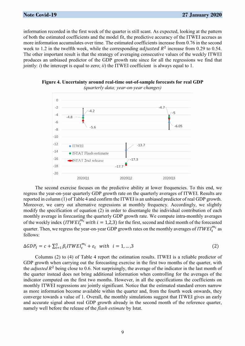
We present a real-time out-of-sample nowcasting exercise during Covid-19 pandemic using ITWEI to predict the year-on-year real GDP growth rate. For the first quarter of 2020 the point forecast, with information up to March 202014, was a -4.2% fall against the -4.8% realized value according to the flash estimate published by Istat (-5.4% the 2nd release; Figure 4). Considering the estimation uncertainty, the 95% confidence bands15 around the point forecast ranged from -6.2% to -2.2%.

As for the second quarter, with the information available up to the end of May, ITWEI predicted a drop in economic activity by about -14% y-o-y (within a [-15.8%; -12.2%] confidence band), against -17.3% according to the flash estimate (-17.7% the 2nd release; Figure 4). For the third quarter, the central prediction was -6% (within a [-8%; -4%] band), against a flash estimate of -4.7% (-5.0% the 2nd release; Figure 4). Thus, realized GDP values fell inside confidence bands in the first and third quarters, but not in the second quarter when the drop in economic activity was exceptionally large.

In order to assess the predictive content of the ITWEI indicator for GDP growth in normal times, we carry out some in-sample predictive regressions excluding the Covid-19 period. The first exercise aims at evaluating the ability of ITWEI in predicting GDP growth at the intra-monthly level as the weekly information accumulates over the quarter with data from January 2011 to December 2019. Accordingly, we regress the year-on-year quarterly GDP growth rate (Δ𝐺𝐺𝐺𝐺𝑃𝑃𝑡𝑡) on the flow of information constructed averaging consecutive weekly values of ITWEI (𝐼𝐼𝐼𝐼𝐼𝐼𝐼𝐼𝐼𝐼𝑡𝑡 ��):

Δ𝐺𝐺𝐺𝐺𝑃𝑃𝑡𝑡 = 𝑐𝑐 + 𝛽𝛽𝑤𝑤𝐼𝐼𝐼𝐼𝐼𝐼𝐼𝐼𝐼𝐼𝑡𝑡 �� + 𝜀𝜀𝑡𝑡 𝑤𝑤ℎ𝑒𝑒𝑒𝑒𝑒𝑒 𝐼𝐼𝐼𝐼𝐼𝐼𝐼𝐼𝐼𝐼𝑡𝑡 �� = 1𝑤𝑤∑ 𝐼𝐼𝐼𝐼𝐼𝐼𝐼𝐼𝐼𝐼𝑤𝑤𝑖𝑖=1 𝑖𝑖 𝑎𝑎𝑎𝑎𝑎𝑎 𝑤𝑤 = 1, … ,12 (1)

Columns (1) to (12) in Table 3 show that at the weekly frequency, the ITWEI index enters significantly and with a positive value in all forecasting regressions, except for the first one, when

12 The erratic developments in some weeks of April are likely to reflect some calendar effects, such as Easter holidays. 13 The timeliness of the indicator is confirmed by industrial production data released for April, which surprised forecasters on the upside. This outcome might have reflected two main factors. First, the fraction of the “non-essential” activities suspended by the Prime Ministerial Decree of 22 March 2020 may have been lower than previously estimated, due to both the requests for derogation and changes in the ATECO code towards “essential” activities by a considerable number of companies. Second, expectations about a partial lifting of the restrictions in May could have generated additional demand in the final part of April, especially for the companies already open for the supply of inputs necessary for the reactivation of production. 14 The prediction is obtained in real-time by averaging consecutive weekly values of ITWEI in the forecasted quarter. 15 Confidence bands are computed using the real-time estimated standard error of the regression between the year-on-year GDP growth rate and the ITWEI index aggregated at quarterly frequency. The confidence bands have a 95% coverage since they are obtained as the product between the standard error of the regression (e.g. the one in Table 3) and the 97.5th percentile of the normal distribution.


9

information recorded in the first week of the quarter is still scant. As expected, looking at the pattern of both the estimated coefficients and the model fit, the predictive accuracy of the ITWEI accrues as more information accumulates over time. The estimated coefficients increase from 0.76 in the second week to 1.2 in the twelfth week, while the corresponding 𝑎𝑎𝑎𝑎𝑎𝑎𝑎𝑎𝑎𝑎𝑎𝑎𝑒𝑒𝑎𝑎 𝑅𝑅2 increase from 0.29 to 0.54. The other important result is that the strategy of averaging consecutive values of the weekly ITWEI produces an unbiased predictor of the GDP growth rate since for all the regressions we find that jointly: i) the intercept is equal to zero; ii) the ITWEI coefficient is always equal to 1.

Figure 4. Uncertainty around real-time out-of-sample forecasts for real GDP

(quarterly data; year-on-year changes)

The second exercise focuses on the predictive ability at lower frequencies. To this end, we

regress the year-on-year quarterly GDP growth rate on the quarterly averages of ITWEI. Results are reported in column (1) of Table 4 and confirm the ITWEI is an unbiased predictor of real GDP growth. Moreover, we carry out alternative regressions at monthly frequency. Accordingly, we slightly modify the specification of equation (2) in order to disentangle the individual contribution of each monthly average in forecasting the quarterly GDP growth rate. We compute intra-monthly averages of the weekly index (𝐼𝐼𝐼𝐼𝐼𝐼𝐼𝐼𝐼𝐼𝑡𝑡

𝑚𝑚𝑖𝑖 𝑤𝑤𝑤𝑤𝑎𝑎ℎ 𝑤𝑤 = 1,2,3) for the first, second and third month of the forecasted quarter. Then, we regress the year-on-year GDP growth rates on the monthly averages of 𝐼𝐼𝐼𝐼𝐼𝐼𝐼𝐼𝐼𝐼𝑡𝑡

𝑚𝑚𝑖𝑖 as follows:

Δ𝐺𝐺𝐺𝐺𝑃𝑃𝑡𝑡 = 𝑐𝑐 + ∑ 𝛽𝛽𝑖𝑖𝐼𝐼𝐼𝐼𝐼𝐼𝐼𝐼𝐼𝐼𝑡𝑡𝑚𝑚𝑖𝑖3

𝑖𝑖=1 + 𝜀𝜀𝑡𝑡 𝑤𝑤𝑤𝑤𝑎𝑎ℎ 𝑤𝑤 = 1, … ,3 (2)

Columns (2) to (4) of Table 4 report the estimation results. ITWEI is a reliable predictor of GDP growth when carrying out the forecasting exercise in the first two months of the quarter, with the adjusted 𝑅𝑅2 being close to 0.6. Not surprisingly, the average of the indicator in the last month of the quarter instead does not bring additional information when controlling for the averages of the indicator computed on the first two months. However, in all the specifications the coefficients on monthly ITWEI regressions are jointly significant. Notice that the estimated standard errors narrow as more information become available within the quarter and, from the fourth week onwards, they converge towards a value of 1. Overall, the monthly simulations suggest that ITWEI gives an early and accurate signal about real GDP growth already in the second month of the reference quarter, namely well before the release of the flash estimate by Istat.


10

Table 3. GDP growth and ITWEI: in-sample regressions at weekly frequency

Notes: HAR standard errors computed using the Newey-West estimator. Results starred at 1%, 5% and 10% levels, ***, **, *.

Dependent variable: real GDP growth

(1) (2) (3) (4) (5) (6) (7) (8) (9) (10) (11) (12) 𝐼𝐼𝐼𝐼𝐼𝐼𝐼𝐼𝐼𝐼𝑎𝑎𝐼𝐼12 1.20***

(0.26) 𝐼𝐼𝐼𝐼𝐼𝐼𝐼𝐼𝐼𝐼𝑎𝑎𝐼𝐼11 1.17***










(0.28) 𝐼𝐼𝐼𝐼𝐼𝐼𝐼𝐼𝐼𝐼𝑎𝑎𝐼𝐼1 0.15

(0.17) 𝐶𝐶𝐶𝐶𝑎𝑎𝑎𝑎𝑎𝑎 0.10 0.04 -0.03 -0.03 -0.06 -0.10 -0.10 -0.08 -0.03 -0.02 0.01 -0.02

(0.40) (0.33) (0.32) (0.27) (0.26) (0.27) (0.28) (0.27) (0.25) (0.26) (0.26) (0.26) Observations 36 36 36 36 36 36 36 36 36 36 36 36

R2 0.05 0.31 0.37 0.49 0.56 0.52 0.51 0.55 0.59 0.56 0.53 0.55 Adjusted R2 0.02 0.29 0.36 0.48 0.54 0.51 0.50 0.54 0.58 0.55 0.52 0.54 Residual Std. Error (df = 34)

1.56 1.33 1.26 1.14 1.07 1.10 1.12 1.07 1.03 1.06 1.09 1.07

F Statistic (df = 1; 34) 1.78 15.30*** 20.39*** 32.87*** 42.45*** 37.35*** 35.76*** 41.75*** 48.37*** 43.18*** 38.71*** 41.70***


11

Table 4. GDP growth and ITWEI: in-sample regressions at quarterly and monthly frequency

Notes: HAR standard errors computed using the Newey-West estimator. Results starred at 1%, 5% and 10% levels, ***, **, *.

Dependent variable: real GDP growth

(1) (2) (3) (4) 𝐼𝐼𝐼𝐼𝐼𝐼𝐼𝐼𝐼𝐼𝑎𝑎

𝑄𝑄 1.24***

(0.25) 𝐼𝐼𝐼𝐼𝐼𝐼𝐼𝐼𝐼𝐼𝑎𝑎𝑚𝑚3 -0.44

(0.44) 𝐼𝐼𝐼𝐼𝐼𝐼𝐼𝐼𝐼𝐼𝑎𝑎𝑚𝑚2 0.88** 1.16**

(0.39) (0.52) 𝐼𝐼𝐼𝐼𝐼𝐼𝐼𝐼𝐼𝐼𝑎𝑎𝑚𝑚1 1.25*** 0.39 0.54

(0.25) (0.39) (0.38) 𝐶𝐶𝐶𝐶𝑎𝑎𝑎𝑎𝑎𝑎 -0.05 -0.06 -0.07 -0.08

(0.26) (0.26) (0.25) (0.24) Observations 36 36 36 36 R2 0.57 0.56 0.61 0.62 Adjusted R2 0.56 0.55 0.59 0.59 Residual Std. Error 1.05 (df = 34) 1.06 (df = 34) 1.01 (df = 33) 1.01 (df = 32) F Statistic 45.26*** (df = 1; 34) 43.86*** (df = 1; 34) 25.92*** (df = 2; 33) 17.62*** (df = 3; 32)


12

References

Aladangady, A., S. Aron-Dine, W. Dunn, L. Feiveson, P. Lengermann, and C. Sahm (2019). From Transactions Data to Economic Statistics: Constructing Real-time, High-frequency, Geographic Measures of Consumer Spending (No. w26253). National Bureau of Economic Research. Aprigliano, V., G. Ardizzi and L. Monteforte (2019) Using Payment System Data to Forecast Economic Activity, International Journal of Central Banking, 15(4), 55-80. Aprigliano, V., G. Ardizzi, A. Cassetta, A. Cavallero, S. Emiliozzi, A. Gambini, N. Renzi and R. Zizza (2020) Exploiting payments to track the Italian economic activity: the experience at Banca d’Italia, Banca d’Italia, Occasional Papers, forthcoming. Aprigliano, V. and L. Bencivelli (2013). Ita-coin: a new coincident indicator for the Italian economy, Banca d’Italia, Working Papers, n. 935. Aprigliano, V. (2020) A large Bayesian VAR with a block‐specific shrinkage: A forecasting application for Italian industrial production, Journal of Forecasting, forthcoming. Aprigliano, V. (2020) Short-term forecasting of the quarterly national accounts with novel variables, Banca d’Italia, mimeo. Ardizzi, G., S. Emiliozzi, J. Marcucci and L. Monteforte (2019) News and consumer card payments, Banca d’Italia, Temi di Discussione n. 1233. Ardizzi, G., A. Nobili and G. Rocco (2020) Game changer in payment habits: evidence from daily data during a pandemic, Banca d'Italia, forthcoming. Baffigi, A., R. Golinelli, and G. Parigi (2004). Bridge models to forecast the euro area GDP, International Journal of forecasting, 20(3), 447-460. Baker, S. R., and A. Fradkin (2017). The impact of unemployment insurance on job search: Evidence from Google search data, Review of Economics and Statistics, 99(5), 756-768. Baker, S. R., R. A. Farrokhnia, S. Meyer, M. Pagel, and C. Yannelis (2020). How does household spending respond to an epidemic? consumption during the 2020 Covid-19 pandemic (No. w26949). National Bureau of Economic Research. Bencivelli, L., M. Marcellino and G. Moretti (2017). Forecasting economic activity by Bayesian bridge model averaging, Empirical Economics, 53(1), 21-40. Biancotti, C., A. Rosolia, F. Venditti and G. Veronese (2020). Salviamo i dati economici dal Covid-19, Banca d’Italia, available at: https://www.bancaditalia.it/media/notizie/2020/Biancotti-et-al-13042020.pdf Bodas, D., J. R. García, J. Murillo, M. Pacce, T. Rodrigo, P. Ruiz de Aguirre, C. Ulloa, J. de Dios Romero and H. Valero (2018). Measuring Retail Trade Using Card Transactional Data, BBVA Research. Carlsen, M. and P. E. Storgaard, (2010). Dankort payments as a timely indicator of retail sales in Denmark, Technical report. Carvalho, V. M., S. Hansen, A. Ortiz, J. R. Garcia, T. Rodrigo, S. Rodriguez Mora, and P. Ruiz de Aguirre (2020). Tracking the COVID-19 crisis with high-resolution transaction data, mimeo. Casa, M., G. D’Alessio (2020). Le statistiche della Banca d’Italia nell’epoca del Coronvirus, Banca d’Italia, available at: https://www.bancaditalia.it/media/notizie/2020/Nota-COVID-Statistiche-2020.10.22.pdf

https://www.bancaditalia.it/media/notizie/2020/Biancotti-et-al-13042020.pdf

https://www.bancaditalia.it/media/notizie/2020/Biancotti-et-al-13042020.pdf

https://www.bancaditalia.it/media/notizie/2020/Nota-COVID-Statistiche-2020.10.22.pdf

https://www.bancaditalia.it/media/notizie/2020/Nota-COVID-Statistiche-2020.10.22.pdf


13

Chen, H., W. Qian, and Q. Wen (2020). The impact of the COVID-19 pandemic on consumption: Learning from high frequency transaction data. Available at SSRN 3568574. Chetty, R., J. N. Friedman, N. Hendren, and M. Stepner (2020). How did covid-19 and stabilization policies affect spending and employment? A new real-time economic tracker based on private sector data (No. w27431). National Bureau of Economic Research. Cicala, S. (2020). Early Economic Impacts of COVID-19 in Europe: A View from the Grid. Tech. rep. Online, last accessed: May 6, 2020. University of Chicago. D’Amuri, F. and J. Marcucci (2017). The predictive power of Google searches in forecasting US unemployment, International Journal of Forecasting, 33 (4), 801-816. D’Amuri, F. and E. Viviano (2020). L’impatto di breve periodo del covid-19 sulla ricerca di lavoro, Banca d’Italia, available at: https://www.bancaditalia.it/media/notizie/2020/labsupply_googleITA.pdf Dempster, A. P., N. M. Laird and D. B. Rubin (1977). Maximum Likelihood from Incomplete Data via the EM Algorithm, Journal of the Royal Statistical Society, 39, 1– 22. Duarte, C., P. M. Rodrigues, and A. Rua (2017). A Mixed Frequency Approach to the Forecasting of Private Consumption with ATM/POS Data, International Journal of Forecasting, 33 (1), 61–75. Eraslan, S. and T. Götz (2020). Weekly activity index for the German economy, Deutsche Bundesbank, available at: https://www.bundesbank.de/wai Esteves, P. S. (2009). Are ATM/POS Data Relevant When Nowcasting Private Consumption?, Technical Report. Galbraith, J. W. and G. Tkacz (2018). “Nowcasting with Payments System Data”, International Journal of Forecasting, 34 (2), 366–76. Jardet, C. and B. Meunier (2020). High-frequency data for nowcasting world GDP growth, Banque de France, mimeo Känzig, D., S. Hacioglu and P. Surico (2020). Consumption in the time of Covid-19: Evidence from UK transaction data, mimeo. Lewis, D.J., K. Mertens, and J.H. Stock (2020a). Monitoring Economic Activity in Real Time, Federal Reserve Bank of New York, Economic research, available at: https://libertystreeteconomics.newyorkfed.org/2020/03/monitoring-real-activity-in-real-time- the-weekly-economic-index.html Lewis, D.J., K. Mertens, J.H. Stock and M. Trivedi (2020b). Measuring Real Activity Using a Weekly Economic Index (No. 920). Federal Reserve Bank of New York. Locarno, A., and R. Zizza (2020). Forecasting in the time of Coronavirus, Banca d’Italia, available at: https://www.bancaditalia.it/media/notizia/forecasting-in-the-time-of-coronavirus Rua, A., and N. Lourenço (2020). The DEI: tracking economic activity daily during the lockdown, (No. w202013) Banco de Portugal. Stock, J. H. and M. W. Watson (2002). Macroeconomic Forecasting Using Diffusion Indexes, Journal of Business & Economic Statistics, 20:2, 147–162. Stock, J.H. and M.W. Watson (2016). Dynamic Factor Models, Factor-Augmented Vector Autoregressions, and Structural Vector Autoregressions in Macroeconomics, Handbook of Macroeconomics, in: J. B. Taylor & Harald Uhlig (ed.), Handbook of Macroeconomics, Elsevier. Verbaan, R., W. Bolt and C. van der Cruijsen (2017). Using debit card payments data for nowcasting Dutch household consumption, De Nederlandsche Bank NV Working Paper, 571.

https://www.bancaditalia.it/media/notizie/2020/labsupply_googleITA.pdf

https://www.bundesbank.de/wai

https://libertystreeteconomics.newyorkfed.org/2020/03/monitoring-real-activity-in-real-time-%20the-weekly-economic-index.html

https://libertystreeteconomics.newyorkfed.org/2020/03/monitoring-real-activity-in-real-time-%20the-weekly-economic-index.html

https://www.bancaditalia.it/media/notizia/forecasting-in-the-time-of-coronavirus


14

Woloszko, N. (2020). Tracking activity in real time with Google Trends, OECD Economics Department Working Papers, No. 1634, OECD Publishing, Paris, https://doi.org/10.1787/6b9c7518-en.

https://doi.org/10.1787/6b9c7518-en

https://doi.org/10.1787/6b9c7518-en

tracking economic growth during the covid-19: a …

Documents