BANCO CENTRAL DE RESERVA DEL PERÚ

Tracking the Exchange Rate Management in Latin America

César Carrera*

* Banco Central de Reserva del Perú

DT. N° 2014-020 Serie de Documentos de Trabajo

Working Paper series Diciembre 2014

Los puntos de vista expresados en este documento de trabajo corresponden a los autores y no reflejan

necesariamente la posición del Banco Central de Reserva del Perú.

The views expressed in this paper are those of the authors and do not reflect necessarily the position of the Central Reserve Bank of Peru.

Tracking the Exchange Rate Management in

Latin America

CÉSAR CARRERA†

Banco Central de Reserva del Perú

This version: July 2013

Abstract:

The exchange rate is one of the most important prices in any open economy. Tracking deviations from

its long-run value may provide important information for policymakers. One way to track such

deviations is to compute the distribution of exchange-rate observed values and compare them with

those of Benford’s law. I document such cases for 15 Latin American countries, for the two most

widely traded currencies. Latin American countries are small open economies that are characterized

for having different degrees of dollarization and intervention in the forex market. This is an

alternative view of how these characteristics play a role with respect to an implied equilibrium

exchange rate.

JEL Classification: C16, F31, F41

Key words: Exchange rate, Forex, Benford’s law.

† I would like to thank Phillipe Bachetta, Lawrence Christiano, Thomas Wu, Diego Winkelried, Adrian Armas,

Nelson Ramirez-Rondan, Sofia and Catherine Carrera, and Hilda Guay for their valuable comments and

suggestions. Maria Robles and Yrasema Dioses provided excellent research assistance. The points of view

expressed throughout this document are the author’s own and are not necessarily shared by the institutions with

which he is currently affiliated.

CÉSAR CARRERA is a Senior Economist in the Research Department, Banco Central de Reserva del Perú, Jr.

Miroquesada 441, Lima, Perú. Email: cesar.carrera@bcrp.gob.pe

2

1. INTRODUCTION

The exchange rate is a key variable for any open economy because it reflects trading and

financial conditions. The value of exports and imports is subject to the volatility of the

exchange rate. The variability of the exchange rate is also important for the determination of

interest rate parity conditions. In that regard, several open economies suffered crises related

to the value of the dollar. Accepting payment for debt in dollars when revenues and incomes

are in local currency may cause solvency issues if the volatility of the exchange rate is high.

In particular, several Latin American economies experience a phenomenon called

dollarization (common use of the dollar rather than domestic currency for transactions). In

addition, some economies fully replaced their domestic currency and now use U.S. dollars

instead.

The forex (FX) market is the world’s largest and most liquid market, with trillions of

dollars being traded on any given day between millions of parties all around the world. The

2010 Triennial Central Bank Survey, which is conducted by the Bank of International

Settlement (BIS), shows a substantial increase in global foreign exchange market activity.1

According to this survey, the U.S. dollar and the euro are the most widely traded currencies

in the world, especially for spot transactions (see Table 1).

On the other hand, Benford’s law (the law of the first digit or the law of the leading

digits) refers to the frequency distribution of digits in many sources of data. Under this law,

the larger the digit the less frequent this digit is likely to be the first digit. The implied

distribution of first digits can be described on a logarithmic weakly monotonic distribution.

1 Triennial Central Bank Survey: Report on global foreign exchange market activity in 2010. Bank of

International Settlements (BIS).

3

Benford’s law can also be extended for the expected distribution for the second digit and

beyond. For this law to hold, data have to be distributed across multiple orders of magnitude

(for example, the list of numbers that represents the populations of U.S. cities). This law does

not hold if there is any cutoff that excludes a portion of the underlying data above a

maximum or below a minimum value (for example, cities defined as a settlement with a

population between 30,000 and 99,000).

TABLE 1 – TURNOVER IN THE GLOBAL FOREIGN EXCHANGE MARKETS

NOTES: 1/ DAILY AVERAGES IN APRIL, IN BILLIONS OF U.S. DOLLARS. 2/ PERCENTAGE SHARES OF AVERAGE

DAILY TURNOVER IN APRIL (THE SUM OF THE PERCENTAGE SHARES OF INDIVIDUAL CURRENCIES TOTALS

200% INSTEAD OF 100% BECAUSE TWO CURRENCIES ARE INVOLVED IN EACH TRANSACTION). SOURCE: BIS

(2010).

The result of Benford’s law has been found to apply to a wide variety of data sets,

including those of the social sciences. For example, Varian (1972), De Grauwe and Decupere

(1992), El Sehity et al. (2005), and Abrantes-Metz et al. (2011) have all used this law to

check the validity of supported data in economics.

De Grauwe and Decupere (1992) are the only ones who use Benford’s law as a

benchmark for realizations of the exchange rate. Donaldson and Kim (1993), Koedijk and

Stork (1994), and Ley and Varian (1994) demonstrate the existence of price clustering in the

last digit of stock market indices. They also tested for psychological barriers through the

observation of unequal passing values of predetermined digits. De Grauwe and Decupere

(1992) follow this strategy of clustering in the FX market for the USD/DEM and USD/JPY

exchange rates and compare them against the implied distribution in Benford’s law. These

1998 2001 2004 2007 2010

A. Global foreign exchange market turnover 1/

Foreign exchange instruments 1527 1239 1934 3324 3981

Spot transactions 568 386 631 1005 1490

Other options and products 959 853 1303 2319 2491

B. Currency distribution of global foreign exchange market turnover 2/

U.S. dollar 87 90 88 86 85

Euro 38 37 37 39

Other currencies 113 72 75 77 76

4

studies infer that clustering, or unequal observations of various digits, implies that

psychological barriers exist.2

In the case of Latin American countries, the application of exchange rate policies is

heterogeneous. In the presence of a crisis, policymakers reacted with measures that range

from exchange rate bands to open market operations. In that regard, I depart from De Grauwe

and Decupere (1992) and argue that the implied Benford’s law distribution can be used as a

benchmark of long-run misalignments that those policies generate. Rather than using

Abrantes-Metz and coauthors’ (2011) strategy of a stable period as a benchmark, I use the

euro exchange rate as a benchmark for the U.S. dollar exchange rate.

In this paper, I investigate whether deviations in the exchange rate from the implied

distribution in Benford’s law provides evidence of deviations in the exchange rate from a

long-run equilibrium perspective. In that regard, I use samples from at least 10 years over the

two most traded currencies in the world for 15 Latin American countries in order to be

consistent with a long-run perspective. I basically find that in economies in which exchange

rate policies are more active, deviations from Benford’s law are stronger. This may suggest

that these policies tend to distort this relative price.

The remainder of this paper is organized as follows: Part 2 introduces Benford’s law and

its relationship with data in economics. Part 3 presents the main characteristic of the data.

Part 4 includes an estimation and comparison of each exchange rate distribution versus the

implied Benford’s distribution. Part 5 concludes.

2 Mitchell and Izan (2006) argue that this interpretation is misleading and the evidence found in previous

literature is not strong enough to argue in favour of psicological barriers in the exchange rate market.

5

2. BENFORD’S LAW

In a given data set, Benford (1938) shows that the probability of occurrence of a certain

digit as the first digit decreases logarithmically as the value of the digit increases from 1 to 9.

This observation is known as Benford’s law and holds for data sets in which the occurrence

of numbers is free from any restriction. This result has been probed to hold for a wide variety

of variables.3 This law can be generalized to numbers with a base different than 10, or to

posterior positions of a digit in a number.4

Several studies show that numbers that have been tampered with or are unrelated or

fabricated do not usually follow Benford’s law. Thus, significant deviations from the Benford

implied distribution may indicate unauthorized intervention or fraudulent or corrupted data.

2.1 The first and second digit

Benford’s law implies that the probability of a digit to be the first digit in a numerical

variable is given by:

𝑃𝑟𝑜𝑏(𝑥 = 𝑑) = 𝑙𝑜𝑔10(1 + 𝑑−1) for d = 1, 2, 3, … 9 (1)

where d is the value of the digit.

Equation (1) can be generalized for the probability of being the second digit:

𝑃𝑟𝑜𝑏(𝑥 = 𝑑) = ∑ 𝑙𝑜𝑔10[1 + (10𝑘 + 𝑑)−1]9𝑘=1 for d = 0, 1, 2, 3, … 9 (2)

Equations (1) and (2) imply distributions for the first and second digit of a numerical

variable, respectively (see Table 2 and Figure 1).

3 In Benford (1938), the data from 20 different domains are tested. The original data set included the surface

areas of 335 rivers, the sizes of 3,259 U.S. populations, 104 physical constants, 1,800 molecular weights, 5,000

entries from a mathematical handbook, 308 numbers contained in an issue of Readers’ Digest, the street

addresses of the first 342 persons listed in American Men of Science, and 418 death rates. 4 For details and extensions to Benford’s law, see Gottwald and Nicol (2002), Lolbert (2008), and Clippe and

Ausloos (2012).

6

TABLE 2 – BENFORD’S LAW

FIGURE 1 – BENFORD’S LAW

A: FIRST DIGIT

B: SECOND DIGIT

Digit First digit Second digit

0 0,12

1 0,30 0,11

2 0,18 0,11

3 0,12 0,10

4 0,10 0,10

5 0,08 0,10

6 0,07 0,09

7 0,06 0,09

8 0,05 0,09

9 0,05 0,08

0,00

0,05

0,10

0,15

0,20

0,25

0,30

0,35

1 2 3 4 5 6 7 8 9

0,00

0,02

0,04

0,06

0,08

0,10

0,12

0,14

0 1 2 3 4 5 6 7 8 9

7

2.2 Use of Benford’s law in Economics

Varian (1972) argues that Benford’s law could be used to detect possible fraud in socio-

economic data. If people who make up figures tend to distribute their digits uniformly, then

comparing the frequency of the first-digit distribution with that expected from Benford’s

distribution would show significant differences. Along the same lines, Nigrini (1999) showed

that Benford’s law could be used in auditing as an indicator of accounting and expenses

fraud.

El Sehity et al. (2005) use Benford’s law as a benchmark for price adjustments and for

detecting irregularities in prices. El Sehity et al. (2005) use two facts: (i) retail managers use

psychological pricing to make the prices of goods appear to be just below a round number,

and (ii) the euro was introduced in several cities in 2002. Those facts distorted existing

nominal price patterns while at the same time retaining real prices. The authors find that the

tendency toward psychological prices results in different inflation rates independent of the

price pattern.

Some other works that use Benford’s law and the idea of a psychological barrier in

financial assets are De Grauwe and Decupere (1992), De Ceuster et al. (1998), Aggarwal and

Lucey (2007), and Dorfleitner and Klein (2009). In particular, De Grauwe and Decupere

(1992) cluster the USD/DEM and USD/JPY exchange rates and compare them against

Benford’s law. De Grauwe and Decupere (1992), Ley (1996), and De Ceuster et al. (1998)

argue that Benford’s law describes many data series, including financial data, so that

widespread clustering simply due to the form of the number itself is possible.

Abrantes-Metz and Bajari (2009) study how statistical methods have started to be used in

antitrust and finance to detect a variety of conspiracies and manipulations. Abrantes-Metz et

al. (2011) investigate deviations of the LIBOR from equilibrium values by testing different

8

realizations for different samples (around February 2006) and suggest that those deviations

have as a source the collusion among big commercial banks.

2.3 Equilibrium exchange rate?

The real exchange rate equilibrium value has always been a key issue in international

economics. Views about its behavior range from the short-run market approach to the long-

run power purchasing parity theory. Among all views to derive equilibrium exchange rate

values, the Behavioral Equilibrium Exchange Rate (BEER) approach is one of the most

accepted and is based on a long-run (cointegrating) relationship between the real exchange

rate and economic fundamentals. The BEER value is the predicted exchange rate from the

cointegrating equation. This long-run view is complemented with a vector error correction

model (VECM) that identifies how quickly the real exchange rate converges toward its long-

run equilibrium value.

Dufrénot et al., (2008) argue that the experience of real exchange rates has been

characterized by substantial misalignments, with time lengths much higher than those

suggested by theoretical models. According to the standard view, deviations from the

equilibrium level are temporal because there are forces that ensure mean-reverting dynamics.

Béreau et al. (2010) points out that this relationship can be explained with nonlinear

dynamics and, if so, that exchange rates can spend long periods away from their fundamental

values.

The goal of my paper is to contribute to this literature by providing evidence of such

misalignments process of the exchange rate toward its equilibrium value.

9

3. DATA CHARACTERISTICS

Previous to testing the deviations of the exchange rate from equilibrium values, I describe

first the currencies under inspection and then describe the two exchange rates. In the next

section, I use these results to test the deviations from the distribution implied by Equation (2).

In this paper, “exchange rate” refers to the spot exchange rate.5 For most countries in this

sample, this variable is also known as the interbank exchange rate. The data are taken from

Bloomberg and at daily frequency. For most countries, the data for the U.S. dollar exchange

rate became available beginning in 1993. Some other countries have data available starting in

1994. Data for the euro exchange rate begin in 1999.

3.1 Latin American currencies

In Latin American countries, exchange rate policies refer to the U.S. dollar. For most

Latin American countries during the 1990s, the exchange rate policy was characterized by an

exchange rate target zone that takes the form of a band, i.e., the exchange rate was flexible as

long as it was inside the limits of the band. During the 2000s, a float managed exchange rate

was used. Interventions in the exchange rate market to either influence the exchange rate

inside the band or reduce its volatility have been the common factor in the region.

The northern countries of South America, such as Colombia and Venezuela, followed

fairly different approaches with respect to the exchange rate. In Colombia, during the 90s, the

exchange rate policy was characterized for exchange-rate bands (in some periods with even a

crawling peg in the limit of the band). During the 2000s, the mechanism was direct

5 This is the rate of a foreign exchange contract for immediate delivery. Spot exchange rates are also known as

“benchmark rates” because spot rates represent the price that a buyer expects to pay for a foreign currency in

another currency.

10

intervention. In Venezuela, the exchange rate policy can be characterized as exchange rate

bands (90s) and a fixed exchange rate, which is under review every year (2000s).

Some other countries such as Brazil and Argentina experienced major changes in their

domestic currencies in the 90s. These countries were looking for pegged exchange rates at

equal parity to the U.S. dollar. By the 2000s, they both follow managed float exchange rate

policies.6 Neighboring countries such as Uruguay and Paraguay followed different exchange

rate policies. Uruguay was directly affected by the exchange rate policy in Argentina, and

during the 90s, this country used an exchange rate band, turning to a managed float exchange

rate in the 2000s.

In the Pacific, there were also mixed policies. While Chile used a band during the 90s and

then switched to a managed float exchange rate, Peru primarily used a managed float

exchange rate in which interventions were aimed at the reduction in the volatility of the

exchange rate. On the other hand, Ecuador used direct interventions, with a central bank

fixing the exchange rate. In 1994, the country had a managed float exchange rate; in 1995, it

used exchange rate bands; and it began using a full dollarization program in 2000.7

In Central America, there were also mixed exchange rate policies. In Guatemala and the

Dominican Republic, the exchange rate was fixed (crawling peg) by the government (in the

90s) and a managed float policy was instituted thereafter (2000s). Costa Rica adopted the

crawling-peg policy (in the 90s and the mid-2000s) and then crawling bands. El Salvador

used a fixed exchange rate (during the 90s) and, since January 2001, the U.S. dollar has

become that country’s legal tender.8

6 In the case of Argentina, from January 1992 to January 2002 (this period is known as Plan de Convertibilidad),

1 peso equaled 1 U.S. dollar. Since then it has been allowed to float freely. The official Brazilian rate, from

October 1993 to January 1999 (plan Real), was 1 real equals 1 U.S. dollar. Since January 1999, the official rate

has been the managed float exchange rate. 7 On March 13, 2000, the Ecuadorian National Congress approved a new exchange system whereby the U.S.

dollar was adopted as the main legal tender in Ecuador for all purposes; on March 20, 2000, the Central Bank of

Ecuador started to exchange sucres for U.S. dollars at a fixed rate of 25,000 sucres per U.S. dollar; and since

April 30, 2000, all transactions have been denominated in U.S. dollars. 8 The exchange rate was then fixed at 8.75 colones per U.S. dollar. Since 1993, the rate has been fixed at 8.755.

11

At the beginning of the 1990s, Mexico used a band policy, with a fixed lower bound and

a crawling peg in the upper bound. Later on (in 1994) the band scheme was abandoned, and

Mexico entered into a scheme of a managed float exchange rate.

3.2 The U.S. dollar and the euro

The first and foremost traded currency in the world is the U.S. dollar. This currency can

be found in a pair with any currency and often acts as the intermediary in triangular currency

transactions. In addition, the U.S. dollar is used by some countries as the official currency

(dollarization) and is widely accepted in other nations, acting as an alternative form of

payment (partial dollarization). The U.S. dollar is also a benchmark or target rate for

countries that choose to fix or peg their currencies in order to stabilize their exchange rates.

The euro was introduced into world markets on January 1, 1999, and it is the official

currency of the majority of nations within the eurozone. Despite being a new currency, the

euro has quickly become the second most traded currency and the world’s second largest

reserve currency. As a matter of fact, many nations within Europe and Africa peg their

currencies to the euro to stabilize their exchange rates. With the euro being a widely used and

trusted currency, it is very prevalent in the FX market and adds liquidity to any currency pair

it trades within.

4. ESTIMATIONS AND EMPIRICS

The distribution implied in Benford’s law can be thought of as a benchmark that permits

identification of the deviation in the realization of a variable from equilibrium values. In the

absence of any intervention, the exchange rate should reflect fundamental conditions.

12

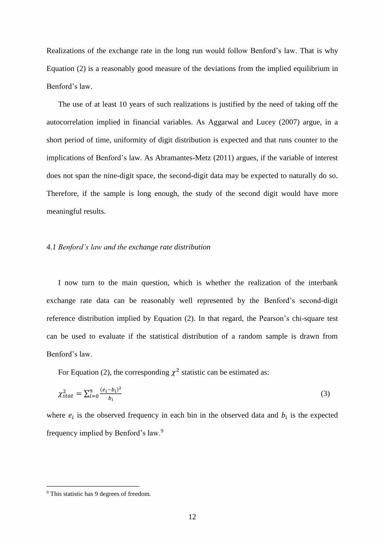
Realizations of the exchange rate in the long run would follow Benford’s law. That is why

Equation (2) is a reasonably good measure of the deviations from the implied equilibrium in

Benford’s law.

The use of at least 10 years of such realizations is justified by the need of taking off the

autocorrelation implied in financial variables. As Aggarwal and Lucey (2007) argue, in a

short period of time, uniformity of digit distribution is expected and that runs counter to the

implications of Benford’s law. As Abramantes-Metz (2011) argues, if the variable of interest

does not span the nine-digit space, the second-digit data may be expected to naturally do so.

Therefore, if the sample is long enough, the study of the second digit would have more

meaningful results.

4.1 Benford’s law and the exchange rate distribution

I now turn to the main question, which is whether the realization of the interbank

exchange rate data can be reasonably well represented by the Benford’s second-digit

reference distribution implied by Equation (2). In that regard, the Pearson’s chi-square test

can be used to evaluate if the statistical distribution of a random sample is drawn from

Benford’s law.

For Equation (2), the corresponding 𝜒2 statistic can be estimated as:

𝜒𝑠𝑡𝑎𝑡2 = ∑

(𝑒𝑖−𝑏𝑖)2

𝑏𝑖

9𝑖=0 (3)

where 𝑒𝑖 is the observed frequency in each bin in the observed data and 𝑏𝑖 is the expected

frequency implied by Benford’s law.9

9 This statistic has 9 degrees of freedom.

13

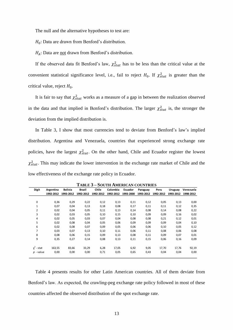
The null and the alternative hypotheses to test are:

𝐻0: Data are drawn from Benford’s distribution.

𝐻𝐴: Data are not drawn from Benford’s distribution.

If the observed data fit Benford’s law, 𝜒𝑠𝑡𝑎𝑡2 has to be less than the critical value at the

convenient statistical significance level, i.e., fail to reject 𝐻0. If 𝜒𝑠𝑡𝑎𝑡2 is greater than the

critical value, reject 𝐻0.

It is fair to say that 𝜒𝑠𝑡𝑎𝑡2 works as a measure of a gap in between the realization observed

in the data and that implied in Benford’s distribution. The larger 𝜒𝑠𝑡𝑎𝑡2 is, the stronger the

deviation from the implied distribution is.

In Table 3, I show that most currencies tend to deviate from Benford’s law’s implied

distribution. Argentina and Venezuela, countries that experienced strong exchange rate

policies, have the largest 𝜒𝑠𝑡𝑎𝑡2 . On the other hand, Chile and Ecuador register the lowest

𝜒𝑠𝑡𝑎𝑡2 . This may indicate the lower intervention in the exchange rate market of Chile and the

low effectiveness of the exchange rate policy in Ecuador.

TABLE 3 – SOUTH AMERICAN COUNTRIES

Table 4 presents results for other Latin American countries. All of them deviate from

Benford’s law. As expected, the crawling-peg exchange rate policy followed in most of these

countries affected the observed distribution of the spot exchange rate.

Digit Argentina Bolivia Brazil Chile Colombia Ecuador Paraguay Peru Uruguay Venezuela

1992-2012 1993-2012 1992-2012 1992-2012 1992-2012 1993-2000 1993-2012 1992-2012 1993-2012 1998-2012

0 0,36 0,29 0,22 0,12 0,13 0,11 0,12 0,05 0,13 0,00

1 0,07 0,04 0,13 0,18 0,08 0,17 0,11 0,11 0,12 0,35

2 0,02 0,04 0,05 0,11 0,13 0,14 0,08 0,14 0,08 0,22

3 0,02 0,03 0,05 0,10 0,15 0,10 0,09 0,09 0,16 0,02

4 0,02 0,05 0,03 0,07 0,04 0,08 0,08 0,21 0,12 0,01

5 0,02 0,08 0,04 0,05 0,06 0,09 0,09 0,09 0,04 0,10

6 0,02 0,08 0,07 0,09 0,05 0,06 0,06 0,10 0,05 0,12

7 0,03 0,07 0,13 0,10 0,11 0,06 0,11 0,08 0,06 0,08

8 0,08 0,06 0,15 0,09 0,13 0,08 0,11 0,09 0,07 0,01

9 0,35 0,27 0,14 0,08 0,13 0,11 0,15 0,06 0,16 0,09

χ2 - stat 163,55 83,66 33,29 6,28 17,05 6,92 9,05 17,70 17,76 92,19

p - value 0,00 0,00 0,00 0,71 0,05 0,65 0,43 0,04 0,04 0,00

14

TABLE 4 – OTHER LATIN AMERICAN COUNTRIES

4.2 The euro: A Benchmark

A natural extension of this analysis is to make homogeneous samples for all countries.

First of all, I estimate the exchange rate against the U.S. dollar for the period from 1994

through 2012. Then, I calculate a similar distribution for the euro spot exchange rate. Given

the fact that the euro appeared in 1999, I re-estimate the distribution of the U.S. exchange rate

for the sample period. Finally, I re-estimate the distribution of the U.S. and the euro exchange

rate for sample periods at least 10 years longer.

Table 5 presents the outcome from the homogeneous sample period for all countries. In

the case of the U.S. dollar for 1994 to 2012, the results slightly differ from the whole sample

analysis. There are no surprises here. When the euro exchange rate is considered, Benford’s

law holds for most countries. This fact may have support from the little intervention in the

euro exchange rate market. In order to make a reasonable comparison between these two

currencies, I consider a similar sample for the U.S. exchange rate. Only Chile and Paraguay

have exchange rate distributions in line with the distribution suggested by Benford’s law.

Digit Costa Rica Dominican Rep. El Salvador Guatemala Mexico

1994-2012 1993-2012 1993-2012 1993-2012 1992-2012

0 0,17 0,02 0,00 0,09 0,25

1 0,19 0,02 0,00 0,05 0,22

2 0,08 0,10 0,00 0,05 0,13

3 0,06 0,13 0,00 0,05 0,14

4 0,05 0,09 0,00 0,02 0,07

5 0,08 0,17 0,00 0,08 0,05

6 0,06 0,20 0,02 0,19 0,03

7 0,07 0,13 0,98 0,19 0,03

8 0,09 0,08 0,00 0,17 0,04

9 0,14 0,07 0,00 0,13 0,04

χ2 - stat 17,37 34,96 957,48 48,16 42,91

p - value 0,04 0,00 0,00 0,00 0,00

15

TABLE 5 – EXCHANGE RATE AND BENFORD’S LAW

In the case of the U.S. dollar, there are differences, even if small, when the sample is

reduced. The 𝜒𝑠𝑡𝑎𝑡2 , which is my measure of the gap between distributions, suggests that

fewer years of observations may distort the original results. Therefore, it is worth it to

observe the evolution of the 𝜒𝑠𝑡𝑎𝑡2 in a sample period that has at least 10 years’ worth of

observations and still stay in the long-run view of the exchange rate.

Table 6 provides the 𝜒𝑠𝑡𝑎𝑡2 for the U.S. exchange rate for samples of 14, 13, 12, 11, and 10

years. From Table 6 it is possible to infer that for most countries, Benford’s law does not

hold. Some countries have a bigger gap than others, some countries keep experiencing an

increasing upward trend, and some countries tend to reduce this gap. At the margin, some

countries sort of have a fixed exchange rate, which clearly differs from Benford’s law.

On the other hand, Table 7 shows a similar comparison for the euro exchange rate. In this

case, Benford’s law holds for most countries at different sample sizes. The absence of an

explicit exchange rate policy with respect to the euro may explain this result.

U.S. Dollar (1994-2012) Euro (1999-2012) U.S. Dollar (1999-2012)

χ2 - stat p - value χ2 - stat p - value χ2 - stat p - value

Argentina 140,26 0,00 13,86 0,13 103,11 0,00

Bolivia 85,80 0,00 38,84 0,00 112,34 0,00

Brazil 29,09 0,00 22,16 0,01 29,11 0,00

Chile 8,07 0,53 2,99 0,96 4,92 0,84

Colombia 19,23 0,02 13,16 0,16 36,38 0,00

Paraguay 8,88 0,45 5,18 0,82 6,88 0,65

Peru 22,46 0,01 13,49 0,14 35,62 0,00

Uruguay 17,56 0,04 7,89 0,55 29,77 0,00

Venezuela 47,62 0,00 92,33 0,00

Costa Rica 17,37 0,04 8,62 0,47 22,05 0,01

Dominican Republic 35,24 0,00 12,17 0,20 40,03 0,00

El Salvador 960,39 0,00 70,45 0,00 956,83 0,00

Guatemala 47,72 0,00 46,60 0,00 60,60 0,00

Mexico 33,63 0,00 17,23 0,05 73,53 0,00

16

TABLE 6 – U.S. EXCHANGE RATE AND BENFORD’S LAW

TABLE 7 – EURO EXCHANGE RATE AND BENFORD’S LAW

In Figure 2, I present the behavior of the 𝜒𝑠𝑡𝑎𝑡2 for the case of the U.S. dollar. There are a

couple of countries well inside the region of Benford’s law (Chile and Paraguay); there are a

couple more that have a clear tendency to reach this threshold (Dominican Republic and

Peru, Figure 2A); and there are a couple of countries that reach this area and then tend to

diverge (Brazil and Costa Rica, Figure 2B).

1999-2012 2000-2012 2001-2012 2002-2012 2003-2012

χ2 - stat p - value χ2 - stat p - value χ2 - stat p - value χ2 - stat p - value χ2 - stat p - value

Argentina 103,11 0,00 89,98 0,00 67,91 0,00 53,57 0,00 70,25 0,00

Bolivia 112,34 0,00 122,48 0,00 139,96 0,00 175,49 0,00 202,65 0,00

Brazil 29,11 0,00 24,33 0,00 16,10 0,06 20,81 0,01 26,60 0,00

Chile 4,92 0,84 4,33 0,89 4,79 0,85 5,23 0,81 8,29 0,50

Colombia 36,38 0,00 38,77 0,00 46,62 0,00 47,47 0,00 50,87 0,00

Paraguay 6,88 0,65 6,41 0,70 11,07 0,27 14,37 0,11 15,58 0,08

Peru 35,62 0,00 35,17 0,00 25,34 0,00 23,61 0,00 23,78 0,00

Uruguay 29,77 0,00 36,62 0,00 50,53 0,00 53,38 0,00 67,88 0,00

Venezuela 92,33 0,00 106,73 0,00 134,05 0,00 168,59 0,00 212,07 0,00

Costa Rica 22,05 0,01 23,71 0,00 17,50 0,04 27,19 0,00 38,45 0,00

Dominican Republic 40,03 0,00 35,70 0,00 32,88 0,00 26,13 0,00 21,43 0,01

El Salvador 956,83 0,00 992,84 0,00 1006,78 0,00 1006,78 0,00 1006,78 0,00

Guatemala 60,60 0,00 64,92 0,00 58,01 0,00 55,07 0,00 51,63 0,00

Mexico 73,53 0,00 85,12 0,00 103,86 0,00 116,81 0,00 127,21 0,00

1999-2012 2000-2012 2001-2012 2002-2012 2003-2012

χ2 - stat p - value χ2 - stat p - value χ2 - stat p - value χ2 - stat p - value χ2 - stat p - value

Argentina 13,86 0,13 20,53 0,01 14,53 0,10 11,65 0,23 9,95 0,35

Bolivia 38,84 0,00 42,32 0,00 51,41 0,00 54,25 0,00 60,97 0,00

Brazil 22,16 0,01 28,23 0,00 21,65 0,01 30,44 0,00 39,69 0,00

Chile 2,99 0,96 4,42 0,88 3,04 0,96 4,08 0,91 3,10 0,96

Colombia 13,16 0,16 12,83 0,17 7,43 0,59 6,99 0,64 7,08 0,63

Paraguay 5,18 0,82 5,81 0,76 5,24 0,81 5,72 0,77 6,41 0,70

Peru 13,49 0,14 20,32 0,02 18,53 0,03 15,01 0,09 20,97 0,01

Uruguay 7,89 0,55 8,56 0,48 9,08 0,43 14,73 0,10 12,16 0,20

Venezuela 47,62 0,00 33,02 0,00 22,53 0,01 17,29 0,04 18,33 0,03

Costa Rica 8,62 0,47 5,11 0,82 2,95 0,97 1,56 1,00 0,98 1,00

Dominican Republic 12,17 0,20 12,17 0,20 8,20 0,51 4,69 0,86 6,17 0,72

El Salvador 70,45 0,00 79,86 0,00 98,53 0,00 121,22 0,00 159,00 0,00

Guatemala 46,60 0,00 56,07 0,00 66,77 0,00 76,66 0,00 93,77 0,00

Mexico 17,23 0,05 23,15 0,01 27,65 0,00 34,14 0,00 45,77 0,00

17

FIGURE 2 – 𝝌𝒔𝒕𝒂𝒕𝟐

FOR THE U.S. DOLLAR

A:

B:

In Figure 3, the 𝜒𝑠𝑡𝑎𝑡2 for the case of the euro is clearly inside the threshold of Benford’s

law. In the cases of Mexico and Brazil, the gap tends to increase as the sample considers a

fewer number of years (Figure 3A). Surprisingly, as the sample is reduced, Benford’s law

tends to hold for Venezuela (Figure 3B).

0

5

10

15

20

25

30

35

40

45

1999-2012 2000-2012 2001-2012 2002-2012 2003-2012

Brazil Chile Paraguay Costa Rica Benchmark

0

5

10

15

20

25

30

35

40

45

1999-2012 2000-2012 2001-2012 2002-2012 2003-2012

Chile Paraguay Peru Dominican Republic Benchmark

18

FIGURE 3 – 𝝌𝒔𝒕𝒂𝒕𝟐

FOR THE EURO

A:

B:

4.3 Deviations from Benford reference distribution

Numerous factors may explain temporal misalignments: transaction costs, heterogeneity

of buyers and sellers, speculative attacks on currencies, the presence of target zones, noisy

traders causing abrupt changes, and the heterogeneity of central banks’ interventions. All

these factors imply either a relationship between the exchange rate and the economic

fundamentals or an adjustment mechanism with time-dependent properties.

0

5

10

15

20

25

30

35

40

45

50

1999-2012 2000-2012 2001-2012 2002-2012 2003-2012

Brazil Chile Colombia

Paraguay Uruguay Costa Rica

Dominican Republic Mexico Benchmark

0

5

10

15

20

25

30

35

40

45

50

1999-2012 2000-2012 2001-2012 2002-2012 2003-2012

Argentina Chile Colombia Paraguay

Peru Uruguay Venezuela Costa Rica

Dominican Republic Benchmark

19

Here, I consider a period long enough that the adjustment process can be viewed as a

short-run deviation from the fundamentals of the economy. The detected processes here help

at modeling asymmetries inherent to the adjustment process. This is particularly interesting

because these asymmetries may explain, for instance, the unequal durations of

undervaluations and overvaluations. Here, all I can say is that there are deviations from a

long-run equilibrium exchange rate perspective, and these deviations seem to be stronger in

some cases, even though a flexible exchange regime is in place.

5. CONCLUSIONS

I use Benford’s law to compare the realization of the exchange rate with respect to long-

run implied equilibrium realizations of the U.S. dollar exchange rate. Benford’s implied

distribution can be viewed as a reasonable alternative to structural models of the fundamental

exchange rate to detect deviations from a long-run perspective. Deviations from this implied

distribution may be reflecting factors such as transaction costs, changing regimes

fluctuations, or open market operations. Moreover, such an approach helps to understand

delays that are inherent to the adjustment process. This is particularly interesting because

these delays may explain the unequal likelihood of undervaluations or overvaluations. As a

second step, I make a comparison against a currency that has a less active monetary policy:

the euro.

In the case of the U.S. dollar, Benford’s law holds for two countries (Chile and

Paraguay); however, in the case of the euro, the law seems to hold for most Latin American

countries. Although the U.S. dollar is important for most transactions in these economies and

there are explicit policies associated with it, the euro has become an important currency and

20

an alternative to the U.S. dollar in these countries as well, even though there are not active

policies regarding the exchange rate observed in the market.

Finally, I find that the gap for this law to hold true became lower in the U.S. dollar

exchange rate market for the case of Dominican Republic and Peru, which suggests that if the

exchange rate is deviated, this deviation seems not to hold under a long-run perspective.

REFERENCES

Abrantes-Metz, R., Villas-Boas, S., Judge, G., 2011. Tracking the Libor rate. Applied

Economic Letters 18, 893 – 899.

Abrantes-Metz, R., Bajari, P., 2009. Screens for conspiracies and their multiple applications.

Antitrust Magazine, December.

Aggarwal, R., Lucey, B., 2007. Psychological barriers in gold prices? Review of Financial

Economics, 16, 217–230

Benford, F., 1938. The Law of Anamalous Numbers. Proceedings of the American

Philosophy Society, 78, 551 – 572.

Béreau, S., López, A., Mignon, V., 2010. Nonlinear adjustment of the real exchange rate

towards its equilibrium value: A panel smooth transition error correction modeling.

Economic Modelling, 27, 404–416.

Clippe, P., Ausloos, M., 2012. Benford’s law and Theil transform of financial data. Physica

A, 391, 6556–6567.

De Ceuster, M., Dhaene, G., Schatteman, T., 1998. On the hypothesis of psychological

barriers in stock markets and Benford’s Law. Journal of Empirical Finance, 5, 263–279

De Grauwe, P., Decupere, D., 1992. Psychological barriers in the foreign exchange market.

Journal of International and Comparative Economics 1, 87–101.

Donaldson, R., Kim, H., 1993. Price barriers in the Dow Jones Industrial Average. Journal of

Financial and Quantitative Analysis 28 (3), 313–330.

Dufrénot, G., Lardic, S., Mathieu, L., Mignon, V., Péguin-Feissolle, A., 2008. Explaining the

European exchange rates deviations: long memory or non-linear adjustment? Journal of

International Financial Markets, Institutions & Money 18 (3), 207–215.

Dorfleitner, G., Klein, C., 2009. Psychological barriers in European stock markets: Where are

they? Global Finance Journal 19, 268–285.

21

El Sehity, T., Hoelzl, E., Kirchler, E., 2005. Price developments after a nominal shock:

Benford’s law and psychological pricing after the euro introduction. International Journal of

Research in Marketing, 22, 471–80.

Gottwald, G., Nicol, M., 2002. On the nature of Benford’s Law. Physica A, 303, 387–396.

Koedijk, K., Stork, P., 1994. Should we care? Psychological barriers in stock markets.

Economics Letters, 44 (4), 427–432.

Ley, E., 1996. On the peculiar distribution of the U.S. stock indexes’ digits. American

Statistician, 50 (4), 311–313.

Ley, E.,Varian, H., 1994. Are there psychological barriers in the Dow-Jones Index? Applied

Financial Economics, 4 (3), 217–224.

Lolbert, T., 2008. On the non-existence of a general Benford’s law. Mathematical Social

Sciences, 55, 103–106.

Mitchell, J., Izan, H., 2006. Clustering and psychological barriers in exchange rates. Journal

of International Financial Markets, Institutions & Money, 16, 318–344.

Nigrini, M., 1999. I’ve got your number. Journal of Accountancy, 187(5), 79-83.

Varian, H., 1972. Benford’s law. American Statistician, 26, 65.