traction control system development for an awd hybrid vehicle
TRANSCRIPT

POLITECNICO DI TORINO
Dipartimento di Ingegneria Meccanica e Aerospaziale
Corso di Laurea Magistrale in Ingegneria Meccanica
Tesi di laurea
Traction Control System development
for an AWD hybrid vehicle
Relatori: Prof. Alessandro Vigliani Ing. Antonio Tota Tutor aziendale: Ing. Salvatore Calanna
Candidata: Roberta Laneve
Dicembre 2020

i
Contents
List of figures ...................................................................................................................................... iii
List of tables ....................................................................................................................................... vii
Acknowledgments ......................................................................................................................... viii
Abstract................................................................................................................................................. ix
1 Introduction ............................................................................................................................... 1
1.1 Thesis structure ............................................................................................................... 3
2 14 DOF Vehicle dynamics ..................................................................................................... 5
2.1 Ride dynamics ................................................................................................................... 5
2.2 Handling dynamics ......................................................................................................... 7
2.3 Handling diagrams ....................................................................................................... 12
2.4 Tire dynamics ................................................................................................................. 19
3 VI–CarRealTime ..................................................................................................................... 24
3.1 Vehicle Model on VI-CarRealTime ......................................................................... 24
3.2 Co-simulation with MATLAB/Simulink................................................................ 36
4 Traction Control System .................................................................................................... 38
4.1 Traction Control action .............................................................................................. 38
4.2 Traction Control Design ............................................................................................. 39
4.2.1 Target longitudinal slip calculation ............................................................. 41
4.2.2 Comfort mode ........................................................................................................ 43
4.2.3 Sport mode ............................................................................................................. 45
4.2.4 Wet mode ................................................................................................................ 47
4.3 PID Controller ................................................................................................................ 48
4.4 Control implementation on MATLAB-Simulink ................................................ 50
5 Simulation tests results ...................................................................................................... 54
5.1 Tests scenario ................................................................................................................ 54
5.2 Comparison with passive vehicle .......................................................................... 57
5.2.1 Mu-split road .......................................................................................................... 57
ii
5.2.2 Variable Mu-split road ........................................................................................ 61
5.2.3 Low friction road .................................................................................................. 64
5.3 Comparison with internal VI-CarRealTime TC system .................................. 67
6 Driving Simulator results ................................................................................................... 71
6.1 Tests executions ............................................................................................................ 72
6.2 Driver feedback .............................................................................................................. 77
7 Conclusions .............................................................................................................................. 79
7.1 Future developments .................................................................................................. 80
Bibliography ...................................................................................................................................... 82

iii
List of figures
Figure 1: 14 DOF vehicle model [17] ........................................................................................ 5
Figure 2: Vehicle ride model (adapted from [18]) .............................................................. 6
Figure 3: Vehicle handling model (adapted from [19]) .................................................... 7
Figure 4: Sprung mass roll equilibrium (adapted from [20]) ........................................ 9
Figure 5: Lateral load transfer (adapted from [20]) ....................................................... 10
Figure 6: Longitudinal load transfer – driving condition (adapted from [20]) ... 11
Figure 7: Bicycle vehicle model cornering (adapted from [22]) ................................ 12
Figure 8: Kinematic steering (adapted from [23]) ........................................................... 13
Figure 9: Dynamic steering (adapted from [21]) ............................................................. 13
Figure 10: Steer angle versus lateral acceleration at constant path curvature
(adapted from [21]) ...................................................................................................................... 15
Figure 11: Understeer gradient evaluation during a ramp-steer manoeuvre ..... 16
Figure 12: Side-Slip angle diagram for a ramp-steer manoeuvre ............................. 17
Figure 13: Static Margin diagram for a ramp-steer manoeuvre ................................ 18
Figure 14: Roll angle and LLTD [%F] diagrams for a ramp-steer manoeuvre .... 19
Figure 15: Wheel free body diagram (adapted from [19]) ........................................... 19
Figure 16: Position of wheel centre of rotation in pure rolling (C), breaking (C')
and traction (C'') condition [23] .............................................................................................. 20
Figure 17: Curves 𝐹𝑥(𝑆) for different load values for a tire 225/50 R 17 [20] .... 21
Figure 18: Curves 𝐹𝑦(𝛼)and 𝑀𝑧(𝛼) for different load values for a tire 225/50 R 17
[20] ....................................................................................................................................................... 22
Figure 19: 𝐹𝑦 − 𝐹𝑥 characteristic for combined slip [21] ............................................. 23
Figure 20: Curve produced by the original sine version of the Magic Formula [21]
................................................................................................................................................................ 23
Figure 21: VI-CarRealTime vehicle model [26] .................................................................. 24
Figure 22: VI-CarRealTime Vehicle Reference System [26] ......................................... 25
Figure 23: Hybrid vehicle powertrain configuration on VI-CarRealTime .............. 27
Figure 24: Rear engine torque-speed map .......................................................................... 27
Figure 25: Differential characteristic during rampsteer manoeuvres (20 deg/s
@100 km/h, 130 km/h, 170 km/h, 200 km/h) .................................................................... 29
Figure 26: Front electric motor torque-speed map ......................................................... 29

iv
Figure 27: Front brake calliper [27] ....................................................................................... 31
Figure 28: Rear brake calliper [27] ......................................................................................... 31
Figure 29: VI-CarRealTime suspension forces evaluation [26] ................................... 32
Figure 30: Toe and Camber angles VI-CarRealTime sign reference .......................... 33
Figure 31: Dampers’ characteristics ....................................................................................... 33
Figure 32: Vehicle’s roll characteristics on a rampsteer manoeuvre (20 𝑑𝑒𝑔/
𝑠 @100 𝑘𝑚/ℎ) .................................................................................................................................. 34
Figure 33: Parallel wheel travel suspension test .............................................................. 34
Figure 34: Vehicle’s handling characteristics on a rampsteer manoeuvre
(20 𝑑𝑒𝑔/𝑠 @100 𝑘𝑚/ℎ) ............................................................................................................... 35
Figure 35: Vehicle's static margin ............................................................................................ 35
Figure 36: VI-CarRealTime model Simulink block (s-function) ................................... 36
Figure 37: Simulink interface for VI-CarRealTime s-function input ports .............. 36
Figure 38: Longitudinal and lateral wheel ground forces as function of
longitudinal slip ............................................................................................................................... 38
Figure 39: General control scheme for each vehicle wheel .......................................... 40
Figure 40: Pacejka 𝐹𝑥0(𝑆) curve of vehicle front wheels ............................................... 42
Figure 41: Influence of wheel vertical load on wheel longitudinal force, for 𝜇 = 1
(front wheels) ................................................................................................................................... 42
Figure 42: Influence of road friction coefficient on wheel longitudinal force, for
𝐹𝑧 = 4000 𝑁 (front wheels) ....................................................................................................... 43
Figure 43: Comfort mode front wheels control scheme ................................................. 44
Figure 44: Comfort mode rear wheels control scheme ................................................... 44
Figure 45: Sport mode front wheels control scheme ....................................................... 45
Figure 46: Sport mode rear wheels control scheme ........................................................ 46
Figure 47: Sport mode yaw-rate control for front wheels ............................................ 47
Figure 48: Wet mode front wheels control scheme ......................................................... 48
Figure 49: Wet mode rear wheels control scheme ........................................................... 48
Figure 50: Block diagram of a process with a feedback controller [32] ................. 49
Figure 51: PID controller structure [32] ............................................................................... 49
Figure 52: Control scheme on MATLAB-Simulink ............................................................. 51
Figure 53: Target wheels longitudinal slips block ............................................................ 51
v
Figure 54: Wheels actual longitudinal slips block ........................................................... 52
Figure 55: Traction Control block ........................................................................................... 52
Figure 56: Traction Control sub-blocks ................................................................................ 53
Figure 57: VI-EventBuilder interface ...................................................................................... 54
Figure 58: Driver throttle demand during acceleration manoeuvre ....................... 55
Figure 59: Road friction coefficients during mu-split manoeuvre ............................ 55
Figure 60: Road friction coefficients on variable mu-split manoeuvre ................... 56
Figure 61: Road friction coefficients during low friction manoeuvre ..................... 56
Figure 62: Wheels longitudinal slips during mu-split test ............................................ 57
Figure 63: Driver steering angle and vehicle longitudinal acceleration during mu-
split test ............................................................................................................................................... 58
Figure 64: Wheels traction torques during mu-split test .............................................. 59
Figure 65: Right wheels normal load during mu-split test ........................................... 59
Figure 66: Driver steering angle and driver steering angle speed during mu-split
test (Sport mode) ............................................................................................................................ 60
Figure 67: Vehicle yaw-rate and longitudinal acceleration during mu-split test
(Sport mode) ..................................................................................................................................... 60
Figure 68: Wheels longitudinal slips during variable mu-split test .......................... 62
Figure 69: Driver steering angle and vehicle longitudinal acceleration during
variable mu-split test .................................................................................................................... 62
Figure 70: Driver steering angle and vehicle longitudinal acceleration during
variable mu-split test (Sport mode) ........................................................................................ 63
Figure 71: Wheels traction torque during variable mu-split test .............................. 64
Figure 72: Wheels longitudinal slips during low friction test ..................................... 64
Figure 73: Driver steering angle and vehicle longitudinal acceleration during low
friction test ........................................................................................................................................ 65
Figure 74: Wheels traction torque during low friction test ......................................... 66
Figure 75: Right wheels normal load during low friction test .................................... 66
Figure 76: Driver steering angle and vehicle longitudinal acceleration during low
friction test (different 𝜇 value estimated) ........................................................................... 67
Figure 77: VI-CarRealTime TCS options for electric motor and engine .................. 67
vi
Figure 78: Comparison of designed TC (Comfort and Sport modes) and VI-CRT TC
on mu-split test: driver steering angle, longitudinal acceleration, wheels
longitudinal slips ............................................................................................................................. 68
Figure 79: Comparison of designed TC (Comfort and Sport modes) and VI-CRT TC
on low friction test: driver steering angle, longitudinal acceleration, wheels
longitudinal slips ............................................................................................................................. 69
Figure 80: Danisi Engineering dynamic driving simulator [34] ................................. 71
Figure 81: Results of mu-split manoeuvre: wheel longitudinal slips, motors and
engine torque, vehicle longitudinal acceleration, driver steering angle, vehicle
trajectory ............................................................................................................................................ 74
Figure 82: Results of low friction manoeuvre: wheel longitudinal slips, motors
and engine torque, vehicle longitudinal acceleration, driver steering angle,
vehicle trajectory............................................................................................................................. 76

vii
List of tables
Table 1: Vehicle parameters ...................................................................................................... 25
Table 2: Passengers and fuel parameters ............................................................................ 26
Table 3: Sprung mass parameters ........................................................................................... 26
Table 4: Transmission Gear Ratios ......................................................................................... 28
Table 5: Acceleration performance targets ......................................................................... 30
Table 6: Brake system characteristics ................................................................................... 31
Table 7: Front and rear suspension characteristics ........................................................ 33
Table 8: Controllers' coefficient before and after on-line tests .................................. 78

viii
Acknowledgments
Desidero ringraziare il Politecnico di Torino e Danisi Engineering per avermi dato
l’opportunità di partecipare ad un interessante progetto, in un anno sicuramente
non poco complesso.
Ringrazio i miei relatori prof. Alessandro Vigliani e ing. Antonio Tota, per i
preziosi suggerimenti e le conoscenze trasmesse.
Grazie al gruppo AVD di Danisi Engineering per avermi accolta in questi mesi, ed
in particolare il mio tutor ing. Salvatore Calanna per avermi guidata con dedizione
e professionalità in questo percorso.

ix
Abstract
The purpose of this thesis work is to design a Traction Control System algorithm
for an All-Wheel-Drive (AWD) hybrid vehicle. Generally, the control aim is to
prevent the driven wheels from spinning in order to guarantee vehicle stability,
especially on slippery roads. In this specific case, the control logic has to be also
adapted for three vehicle driving modes: Comfort, Wet, and Sport. The work is
developed in collaboration with Danisi Engineering company (Nichelino – TO).
First of all, the 14-degrees-of-freedom vehicle model is implemented on the VI-
CarRealTime software, and its overall dynamic performances are evaluated. The
vehicle object of this study is a high-performance one, equipped with two
independent electric motors on front wheels and an internal combustion engine
on rear axle.
The control structure is developed on MATLAB-Simulink environment: starting
from setting general control aims, the differences among the three driving modes
are established. The controller acts on the vehicle powertrain, reducing motors
and engine output torques in case of wheels excessive rotation. Proportional-
Integral (PI) controllers are adopted for torques regulation.
The three Traction Control modes performances are at first assessed through off-
line tests, which consist of co-simulations of VI-CarRealTime and MATLAB-
Simulink environments. The passive and the controlled vehicles are compared on
different scenarios to verify the effectiveness of control action: a straight-line
maximum acceleration manoeuvre is performed on different road conditions,
including constant mu-split, variable mu-split and low friction surfaces. The same
set of scenarios is also used to analyse the differences between the proposed
control and an internal VI-CarRealTime one. Tests’ results show how all the
designed control achieves its task, enhancing vehicle stability and acceleration
performance. Finally, on-line acceleration manoeuvres tests are performed:
vehicle model and control are implemented on a dynamic driving simulator.
During tests executions the driver’s subjective feedback is collected, to evaluate
how the control activation affects driver perception of the vehicle dynamic
behaviour.


1
1 Introduction
In recent decades, vehicle safety and comfort have gathered increasing interest
in the automotive field. For this purpose, over the past years active safety
technologies have been developed and improved: they are systems that actively
intervene in vehicle operations, generally limiting the movement and retarding
the vehicle itself, in order to stabilize its handling response in critical situations
and maintain its steerability. These systems aim to support the driver in difficult
driving conditions preventing accidents and, thus, contributing to road safety [1].
Among them, Traction Control System (TCS), also called Anti Slip Regulation
(ASR), plays an important role: it enhances vehicle’s longitudinal performances
preventing the driving wheels from spinning when the vehicle accelerates
excessively, particularly on low friction roads and during cornering. In fact, the
loss of traction of wheels leads not only to reduced vehicle velocity or
acceleration in the longitudinal direction, but also, due to tire behaviour, to a poor
lateral performance, so it compromises vehicle handling and stability and it does
not react in the way that the driver would generally expect [1]. In this context, it
is clear that TCS action is fundamental; therefore, it started to be implemented
during the 1990s, initially as an expansion of ABS (TCS can be considered the
counterpart of ABS substantially), and nowadays it is widespread in all the
vehicles [2].
Nowadays, new development and improvement of TCS algorithms can be
achieved with vehicles powered, partially or totally, by electric motors: with
Emissions Standards requiring even more significant reductions in vehicle
emissions, automotive constructors show a recent interest in powertrain
electrification. Hybrid Electric Vehicles (HEV) seem to be the most successful
solution, representing the best compromise between high performances demand
and fuel efficiency: the presence of conventional Internal Combustion Engine
(ICE) permits to overcome the autonomy range limits of batteries, which affect
pure Electric Vehicles, and at the same time the electric powertrain allows better
management of engine functioning, optimizing its operation [3][4]. An HEV
Introduction
2
powertrain can be defined as parallel or series: in the first case, both engine and
electric motors power can be used for propulsion because each of them is
connected to the wheels independently; in the other case, the engine charges the
electric motors' batteries through a generator, thus it has no direct connection to
vehicle wheels [3].
The presence of a hybrid electric powertrain architecture, both parallel and
series, influences TCS design: the controller regulates wheels’ longitudinal slips
mainly acting on the wheel driving torque, which is reduced in case of excessive
wheels rotation; torque limiting is achieved acting on different parameters for
ICEs and electric motors.
For vehicles driven by conventional ICEs, TCS usually reduces engine torque
through various methods: regulating the air amount through throttle valve
opening, reducing the injected fuel quantity, modifying the ignition timing,
cutting spark ignition. In addition, TCS can limit the slip also adding a braking
torque contribute, so increasing brake pressure: brake system response to
control activation is faster than engine one and also permits to differentiate the
control of each wheel, but using it excessively leads to a significant reduction of
its lifetime; as a consequence, breaking system intervention can represent only
an adjustment to the control: it is used when driving wheel slip ratio is high, for a
short time, and in conjunction with engine torque regulation to avoid excessive
fuel consumption [5][6]. In [7] a traction controller based only on engine torque
reduction is proposed: it consists of a PID controller, integrated with a fuzzy logic
controller to improve its performance. [8] shows an innovative control, including
PID and ant colony optimization controller to regulate both engine torque and
brake pressure.
With a hybrid powertrain, TCS can exploit the advantages of electric motors: it
permits a direct torque control, which involves a fast torque response, while
thermal engine control includes several delay factors; it is easy to estimate the
output torque value through measuring the motor current; it is possible to
control each wheel independently with the corresponding motor so that the
control can be more effective in case of roads with different friction for left and

Introduction
3
right wheels and vehicle stability and driving comfort are improved [9][10][11].
Several studies present various algorithms to control the electric powertrains. In
[12] a comparison of different control strategies for electric motors is shown: the
authors assess strength and weaknesses of MTTE, PID, H∞, sliding mode
controllers. [13] proposes an explicit nonlinear model predictive control method,
showing the advantages with respect to a PI controller.
As regards 4WD hybrid powertrain, different solutions have been presented to
combine the control of ICE and electric motors: [14] describes a PID controller
improved by a fuzzy logic integration. In [4] an innovative traction control system
combined with the vehicle Energy Management System is proposed: the aim of
this strategy is to provide both proper vehicle traction and optimized fuel
consumption. [15] shows a new sliding mode controller to achieve the maximum
traction force at the wheels.
The present thesis is inserted in this scenario: this work aims to design a TCS
algorithm for a four-wheel-drive Hybrid Vehicle. The vehicle object of this study
is a high performance one, motorized by two independent electric motors on
front wheels and an ICE on rear axle; vehicle dynamic behaviour and
performances can be settled by the driver switching from Comfort driving mode
to Sport or Wet ones. Consequently, the control logic, which is differentiated for
front and rear vehicle axles, has to be adapted to achieve the task of each driving
mode.
The definition of the hybrid vehicle dynamic model and the design of Traction
Control System is part of a project of Danisi Engineering company, located in
Nichelino (TO), which supported the development of the whole work sharing
know-how and resources.
1.1 Thesis structure
The structure of this thesis is illustrated below:
Chapter 2: 14 DOF Vehicle dynamics. Equations of vehicle dynamics are

Introduction
4
explained referring to a 14 DOF vehicle model: ride, handling and tire dynamics
are considered. A paragraph is also dedicated to handling diagrams, which
characterize vehicle behaviour.
Chapter 3: VI–CarRealTime. In this chapter, the implementation of the vehicle
model on VI-CarRealTime software is shown: each vehicle subsystem is
illustrated with the corresponding specifications and targets, and vehicle
performances are assessed. In the last paragraph of the chapter, co-simulation
with MATLAB-Simulink is explained: this method would be used to make the
control communicate with the vehicle model.
Chapter 4: Traction Control System. The development of Traction Control logic
is described: starting from explaining control aims in general, the targets
expected for the three driving modes are defined. Subsequently, the control
structure is illustrated, pointing out the main differences between Comfort, Sport
and Wet mode and how they are expected to affect vehicle behaviour. Huge
attention is given to the controller chosen for this purpose, which is a PID one,
describing how its properties are considered suitable for Traction Control
purpose. Finally, the implementation of the control algorithm on MATLAB-
Simulink is reported.
Chapter 5: Simulation tests results. The three modes of Traction Control are
tested with co-simulations between VI-CarRealTime and MATLAB-Simulink
environments. Firstly, the passive vehicle and the controlled one are compared
on different simulation test scenarios to assess the effectiveness of control action;
three straight-line acceleration manoeuvres are taken into account,
differentiated by road conditions: constant mu-split, variable mu-split, low
friction. The same set of scenarios is used in the second part of the chapter to
analyse the differences between the designed control and an internal VI-
CarRealTime one.
Chapter 6: Driving Simulator results. Vehicle model and control modes are
implemented on a dynamic driving simulator, in order to perform the same off-
line manoeuvres tests and to obtain feedbacks by a human driver about how the
control activation affects vehicle’s dynamic behaviour.
5
2 14 DOF Vehicle dynamics
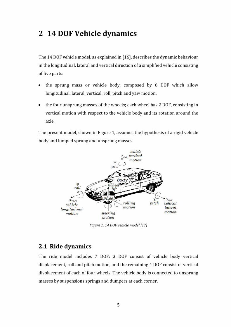
The 14 DOF vehicle model, as explained in [16], describes the dynamic behaviour
in the longitudinal, lateral and vertical direction of a simplified vehicle consisting
of five parts:
• the sprung mass or vehicle body, composed by 6 DOF which allow
longitudinal, lateral, vertical, roll, pitch and yaw motion;
• the four unsprung masses of the wheels; each wheel has 2 DOF, consisting in
vertical motion with respect to the vehicle body and its rotation around the
axle.
The present model, shown in Figure 1, assumes the hypothesis of a rigid vehicle
body and lumped sprung and unsprung masses.
Figure 1: 14 DOF vehicle model [17]
2.1 Ride dynamics
The ride model includes 7 DOF: 3 DOF consist of vehicle body vertical
displacement, roll and pitch motion, and the remaining 4 DOF consist of vertical
displacement of each of four wheels. The vehicle body is connected to unsprung
masses by suspensions springs and dumpers at each corner.

14 DOF Vehicle dynamics
6
Figure 2: Vehicle ride model (adapted from [18])
According to Figure 2, it is possible to define vehicle forces equilibriums
exploiting Newton second law:
• Vehicle sprung mass’ vertical equilibrium:
𝐹𝑠𝑓𝑙 + 𝐹𝑑𝑓𝑙 + 𝐹𝑠𝑓𝑟 + 𝐹𝑑𝑓𝑟 + 𝐹𝑠𝑟𝑙 + 𝐹𝑑𝑟𝑙 + 𝐹𝑠𝑟𝑟 + 𝐹𝑑𝑟𝑟 = 𝑚𝑠�̈�𝑠 (2. 1)
where 𝐹𝑠𝑖𝑗 and 𝐹𝑑𝑖𝑗 are respectively suspensions springs and dumpers forces
for each vehicle corner; each spring is characterized by stiffness 𝑘𝑠𝑖 , while
each dumper is characterized by a dumping coefficient 𝑐𝑠𝑖;
• Vehicle body rotational equilibrium around the 𝑦 axle (pitching moment):
(𝐹𝑠𝑟𝑙 + 𝐹𝑑𝑟𝑙 + 𝐹𝑠𝑟𝑟 + 𝐹𝑑𝑟𝑟)𝑏 − (𝐹𝑠𝑓𝑙 + 𝐹𝑑𝑓𝑙 + 𝐹𝑠𝑓𝑟 + 𝐹𝑑𝑓𝑟)𝑎 = 𝐼𝑝�̈� (2. 2)
• Vehicle body rotational equilibrium around 𝑥 axle (rolling moment):
(𝐹𝑠𝑓𝑙 + 𝐹𝑑𝑓𝑙)𝑡𝑓2+ (𝐹𝑠𝑟𝑙 + 𝐹𝑑𝑟𝑙)
𝑡𝑟2− (𝐹𝑠𝑓𝑟 + 𝐹𝑑𝑓𝑟)
𝑡𝑓2− (𝐹𝑠𝑟𝑟 + 𝐹𝑑𝑟𝑟)
𝑡𝑟2=
= 𝐼𝑟�̈�
(2. 3)

14 DOF Vehicle dynamics
7
• Unsprung masses (wheels) vertical equilibrium:
{
𝐹𝑡𝑓𝑙 − 𝐹𝑠𝑓𝑙 − 𝐹𝑑𝑓𝑙 = 𝑚𝑢𝑓𝑙�̈�𝑢𝑓𝑙𝐹𝑡𝑓𝑟 − 𝐹𝑠𝑓𝑟 − 𝐹𝑑𝑓𝑟 = 𝑚𝑢𝑓𝑟�̈�𝑢𝑓𝑟𝐹𝑡𝑟𝑙 − 𝐹𝑠𝑟𝑙 − 𝐹𝑑𝑟𝑙 = 𝑚𝑢𝑟𝑙�̈�𝑢𝑟𝑙𝐹𝑡𝑟𝑟 − 𝐹𝑠𝑟𝑟 − 𝐹𝑑𝑟𝑟 = 𝑚𝑢𝑟𝑟�̈�𝑢𝑟𝑟
(2. 4)
where 𝐹𝑡𝑖𝑗 are the forces due to tires stiffnesses 𝑘𝑡𝑖 .
2.2 Handling dynamics
The handling model includes 7 DOF: 3 DOF consist of vehicle body longitudinal
and lateral displacement and yaw motion, and the remaining 4 DOF consist of the
rotation of each wheel.
Figure 3: Vehicle handling model (adapted from [19])
In the same way of ride dynamics, vehicle forces equilibriums can be derived from
Figure 3:
• Vehicle’s longitudinal equilibrium:
𝐹𝑥𝑓𝑙 cos 𝛿𝑙 − 𝐹𝑦𝑓𝑙 sin 𝛿𝑙 + 𝐹𝑥𝑓𝑟 cos 𝛿𝑟 − 𝐹𝑦𝑓𝑟 sin 𝛿𝑟 + 𝐹𝑥𝑟𝑙 + 𝐹𝑥𝑟𝑟 +
−1
2𝜌𝐶𝑥𝐴𝑓𝑉𝑥
2sgn𝑉𝑥 = 𝑚𝑎𝑥 (2. 5)
where 𝜌 is the air density, 𝐶𝑥 is the drag coefficient and 𝐴𝑓is the vehicle
frontal area, 𝛿𝑙 and 𝛿𝑟 are respectively the left and right wheel steering
angles. From (2.5), the longitudinal inertial acceleration 𝑎𝑥 at the centre of
gravity can be obtained.

14 DOF Vehicle dynamics
8
• Vehicle’s lateral equilibrium, through which lateral inertial CG acceleration
𝑎𝑦 can be derived:
𝐹𝑥𝑓𝑙 sin 𝛿𝑙 + 𝐹𝑦𝑓𝑙 cos 𝛿𝑙 + 𝐹𝑥𝑓𝑟 sin 𝛿𝑟 + 𝐹𝑦𝑓𝑟 cos 𝛿𝑟 + 𝐹𝑦𝑟𝑙 + 𝐹𝑦𝑟𝑟 = 𝑚𝑎𝑦 (2. 6)
• Vehicle’s rotational equilibrium around the 𝑧 axle (yaw moment):
𝑎(𝐹𝑥𝑓𝑙 sin 𝛿𝑙 + 𝐹𝑦𝑓𝑙 cos 𝛿𝑙 + 𝐹𝑥𝑓𝑟 sin 𝛿𝑟 + 𝐹𝑦𝑓𝑟 cos 𝛿𝑟) +
+𝑡𝑓2(𝐹𝑥𝑓𝑟 cos 𝛿𝑟 − 𝐹𝑦𝑓𝑟 sin 𝛿𝑟 − 𝐹𝑥𝑓𝑙 cos 𝛿𝑙 + 𝐹𝑦𝑓𝑙 sin 𝛿𝑙) +
+𝑡𝑟2(𝐹𝑥𝑟𝑟 − 𝐹𝑥𝑟𝑙) − 𝑏(𝐹𝑦𝑟𝑙 + 𝐹𝑦𝑟𝑟) + 𝑀𝑧𝑓𝑙 +𝑀𝑧𝑓𝑟 +𝑀𝑧𝑟𝑙 +𝑀𝑧𝑟𝑟 = 𝐼𝑧�̈�
(2. 7)
where 𝑀𝑧𝑖𝑗 are the wheel aligning moments. Integrating this equation, it is
possible to obtain the yaw-rate �̇�.
Vehicle velocities can be derived from lateral and longitudinal accelerations and
yaw-rate through the relationships described in (2.8):
{𝑉𝑥 = ∫(𝑎𝑥 +𝑉𝑦�̇�)𝑑𝑡
𝑉𝑦 = ∫(𝑎𝑦 −𝑉𝑥�̇�)𝑑𝑡 (2. 8)
Knowing the two components, vehicle’s overall velocity and side-slip angle can be
calculated:
𝑉 = √𝑉𝑥2 + 𝑉𝑦
2
𝛽 = tan−1𝑉𝑦𝑉𝑥
(2. 9)
Vehicle CG accelerations influence the value of vertical forces which act on each
corner of the vehicle: they cause load transfer between front and rear axles or left
and right vehicle sides, which should be taken into account in the vehicle model.
The presence of a lateral acceleration produced by tire cornering forces generates
an inertial reaction force, called centrifugal force. It causes a roll motion and, as a
consequence, a lateral load transfer. The roll angle 𝜙 can be evaluated through
the moment equilibrium of sprung mass around vehicle roll centre, considering a

14 DOF Vehicle dynamics
9
horizontal roll axis:
𝐼𝑟�̈� + 𝐶�̇� + 𝐾𝜙 = 𝑚𝑎𝑦𝐻𝑟𝑜𝑙𝑙 cos𝜙 +𝑚𝑔𝐻𝑟𝑜𝑙𝑙 sin𝜙 (2. 10)
𝑚𝑎𝑦 = 𝑚𝑎𝑦,𝑅𝐶 + 𝐻𝑟𝑜𝑙𝑙�̈� (2. 11)
Where 𝐾 and 𝐶 are respectively the vehicle total roll stiffness and total roll
damping:
𝐾 = 𝐾𝑓𝑟𝑜𝑛𝑡 + 𝐾𝑟𝑒𝑎𝑟
𝐶 = 𝐶𝑓𝑟𝑜𝑛𝑡 + 𝐶𝑟𝑒𝑎𝑟 (2. 12)
Substituting (2.11) into (2.10),
�̈� =𝑚𝐻𝑟𝑜𝑙𝑙(𝑎𝑦,𝑅𝐶 cos𝜙 + 𝑔 sin𝜙) − 𝐶�̇� − 𝐾𝜙
𝐼𝑟 +𝑚𝐻𝑟𝑜𝑙𝑙2 (2. 13)
Integrating two times (2.13), the roll angle is calculated.
Figure 4: Sprung mass roll equilibrium (adapted from [20])
14 DOF Vehicle dynamics
10
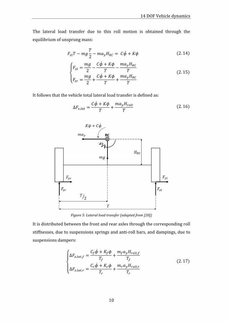
The lateral load transfer due to this roll motion is obtained through the
equilibrium of unsprung mass:
𝐹𝑧𝑙𝑇 −𝑚𝑔𝑇
2−𝑚𝑎𝑦𝐻𝑅𝐶 = 𝐶�̇� + 𝐾𝜙 (2. 14)
{
𝐹𝑧𝑙 =𝑚𝑔
2−𝐶�̇� + 𝐾𝜙
𝑇−𝑚𝑎𝑦𝐻𝑅𝐶
𝑇
𝐹𝑧𝑟 =𝑚𝑔
2+𝐶�̇� + 𝐾𝜙
𝑇+𝑚𝑎𝑦𝐻𝑅𝐶
𝑇
(2. 15)
It follows that the vehicle total lateral load transfer is defined as:
Figure 5: Lateral load transfer (adapted from [20])
It is distributed between the front and rear axles through the corresponding roll
stiffnesses, due to suspensions springs and anti-roll bars, and dampings, due to
suspensions dampers:
{
∆𝐹𝑧,𝑙𝑎𝑡,𝑓 =
𝐶𝑓�̇� + 𝐾𝑓𝜙
𝑇𝑓+𝑚𝑓𝑎𝑦𝐻𝑟𝑜𝑙𝑙,𝑓
𝑇𝑓
∆𝐹𝑧,𝑙𝑎𝑡,𝑟 =𝐶𝑟�̇� + 𝐾𝑟𝜙
𝑇𝑟+𝑚𝑟𝑎𝑦𝐻𝑟𝑜𝑙𝑙,𝑟
𝑇𝑟
(2. 17)
∆𝐹𝑧,𝑙𝑎𝑡 =𝐶�̇� + 𝐾𝜙
𝑇+𝑚𝑎𝑦𝐻𝑟𝑜𝑙𝑙
𝑇 (2. 16)

14 DOF Vehicle dynamics
11
In the same way, the presence of a positive longitudinal acceleration due to
driving traction condition generates an inertial reaction force, which causes a
pitch motion and a longitudinal load transfer:
∆𝐹𝑧,𝑙𝑜𝑛𝑔 =𝑚𝑎𝑥ℎ𝐺𝑙
(2. 18)
Along longitudinal direction, also the aerodynamic resistance causes a
longitudinal load transfer:
∆𝐹𝑧,𝑎𝑒𝑟 =
12𝜌𝐶𝑥𝐴𝑓𝑉𝑥
2sgn𝑉𝑥
𝑙ℎ𝐴 (2. 19)
Figure 6: Longitudinal load transfer – driving condition (adapted from [20])
After adding load transfers to the forces due to static load distribution and
aerodynamic downforce, the overall vertical forces on each vehicle corner are
reported in (2.20):
{
𝐹𝑧𝑓𝑙 =
1
2
𝑚𝑔𝑏
𝑙+1
2(1
2𝜌𝐶𝑧,𝑓𝐴𝑓𝑉𝑥
2) −1
2(∆𝐹𝑧,𝑙𝑜𝑛𝑔 + ∆𝐹𝑧,𝑎𝑒𝑟) − ∆𝐹𝑧,𝑙𝑎𝑡,𝑓
𝐹𝑧𝑓𝑟 =1
2
𝑚𝑔𝑏
𝑙+1
2(1
2𝜌𝐶𝑧,𝑓𝐴𝑓𝑉𝑥
2) −1
2(∆𝐹𝑧,𝑙𝑜𝑛𝑔 + ∆𝐹𝑧,𝑎𝑒𝑟) + ∆𝐹𝑧,𝑙𝑎𝑡,𝑓
𝐹𝑧𝑟𝑙 =1
2
𝑚𝑔𝑎
𝑙+1
2(1
2𝜌𝐶𝑧,𝑟𝐴𝑓𝑉𝑥
2) +1
2(∆𝐹𝑧,𝑙𝑜𝑛𝑔 + ∆𝐹𝑧,𝑎𝑒𝑟) − ∆𝐹𝑧,𝑙𝑎𝑡,𝑟
𝐹𝑧𝑟𝑟 =1
2
𝑚𝑔𝑎
𝑙+1
2(1
2𝜌𝐶𝑧,𝐴𝑓𝑉𝑥
2) +1
2(∆𝐹𝑧,𝑙𝑜𝑛𝑔 + ∆𝐹𝑧,𝑎𝑒𝑟) + ∆𝐹𝑧,𝑙𝑎𝑡,𝑟
(2. 20)
14 DOF Vehicle dynamics
12
2.3 Handling diagrams
Vehicle handling performance, so how the vehicle behaves with respect to a
steering driver demand, has great importance to assess vehicle stability: for this
purpose, some characteristics are used to study it.
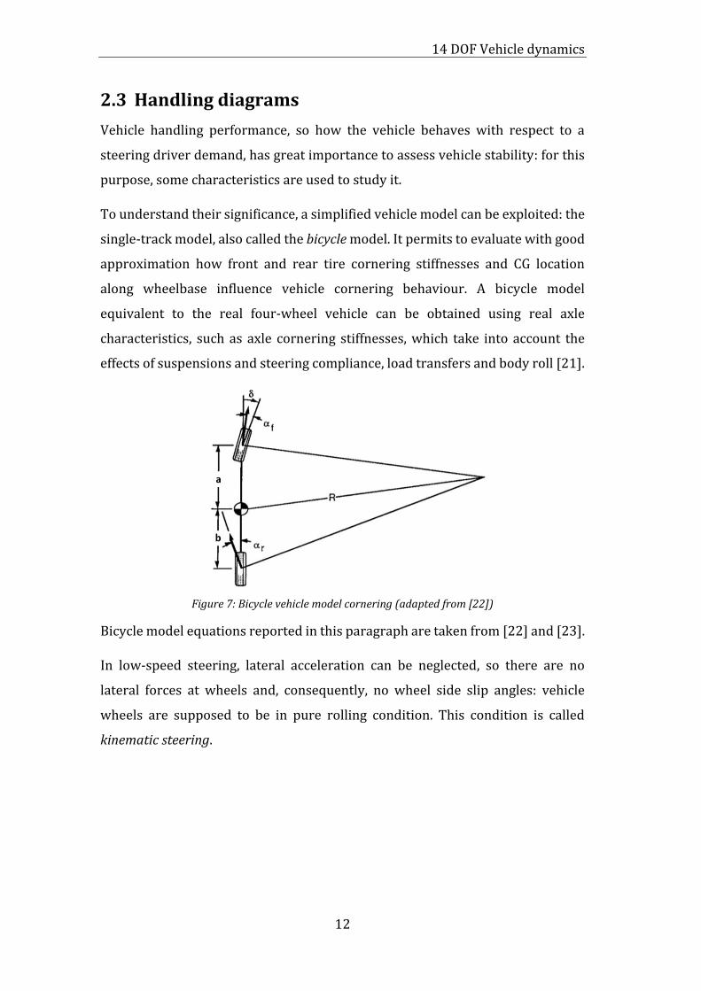
To understand their significance, a simplified vehicle model can be exploited: the
single-track model, also called the bicycle model. It permits to evaluate with good
approximation how front and rear tire cornering stiffnesses and CG location
along wheelbase influence vehicle cornering behaviour. A bicycle model
equivalent to the real four-wheel vehicle can be obtained using real axle
characteristics, such as axle cornering stiffnesses, which take into account the
effects of suspensions and steering compliance, load transfers and body roll [21].
Figure 7: Bicycle vehicle model cornering (adapted from [22])
Bicycle model equations reported in this paragraph are taken from [22] and [23].
In low-speed steering, lateral acceleration can be neglected, so there are no
lateral forces at wheels and, consequently, no wheel side slip angles: vehicle
wheels are supposed to be in pure rolling condition. This condition is called
kinematic steering.

14 DOF Vehicle dynamics
13
Figure 8: Kinematic steering (adapted from [23])
From Figure 8 vehicle scheme, if vehicle wheelbase can be considered negligible
compared to the radius of turn,
𝑅 ≈ 𝑙 cot 𝛿 ≈𝑙
𝛿 ⇒ 𝛿𝑘𝑖𝑛 =
𝑙
𝑅 (2. 21)
𝑅 ≈ 𝑏 cot 𝛽 ≈𝑏
𝛽 ⇒ 𝛽𝑘𝑖𝑛 =
𝑏
𝑅 (2. 22)
When vehicle speed cannot be considered small, a lateral acceleration is present;
as a consequence, wheels have lateral slip angles different from zero and generate
lateral forces: this condition is called dynamic steering.
Figure 9: Dynamic steering (adapted from [21])

14 DOF Vehicle dynamics
14
In a steady-state condition, so when the vehicle is travelling at a constant speed
𝑉, and considering small angles (𝑅 ≫ 𝑙), the forces in lateral direction must
balance the centrifugal force due to lateral acceleration:
𝐹𝑦𝑓 + 𝐹𝑦𝑟 = 𝑚𝑎𝑦 = 𝑚𝑉2
𝑅 (2. 23)
For the moment equilibrium around the centre of gravity,
𝐹𝑦𝑓𝑎 − 𝐹𝑦𝑟𝑏 = 0 ⇒ 𝐹𝑦𝑓 = 𝐹𝑦𝑟𝑏
𝑎 (2. 24)
Substituting (2.24) in lateral equilibrium (2.23),
{
𝐹𝑦𝑟 = 𝑚𝑉2
𝑅
𝑎
𝐿= 𝑚𝑟
𝑉2
𝑅
𝐹𝑦𝑓 = 𝑚𝑉2
𝑅
𝑏
𝐿= 𝑚𝑓
𝑉2
𝑅
(2. 25)
Considering to be in the linear region of the curve 𝐹𝑦(𝛼), which is valid for small
wheel lateral angles, for each axle the lateral force is obtained as the product of
wheel lateral slip angle and the corresponding cornering stiffness:
{𝐹𝑦𝑟 = 𝐶𝛼𝑟𝛼𝑟𝐹𝑦𝑓 = 𝐶𝛼𝑓𝛼𝑓
(2. 26)
Substituting (2.26) in lateral force expression (2.25),
{
𝛼𝑟 =
𝑚𝑟
𝐶𝛼𝑟
𝑉2
𝑅
𝛼𝑓 =𝑚𝑓
𝐶𝛼𝑓
𝑉2
𝑅
(2. 27)
From simple geometrical relationships of vehicle angles,
𝛿 = 𝛿𝑘𝑖𝑛 + 𝛼𝑓 − 𝛼𝑟 (2. 28) Substituting (2.27) in (2.28),
𝛿 − 𝛿𝑘𝑖𝑛 = (𝑚𝑓
𝐶𝛼𝑓−𝑚𝑟
𝐶𝛼𝑟)𝑉2
𝑅= 𝑈𝐺
𝑉2
𝑅 (2. 29)
14 DOF Vehicle dynamics
15
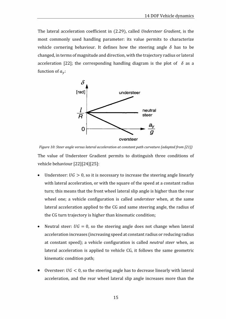
The lateral acceleration coefficient in (2.29), called Understeer Gradient, is the
most commonly used handling parameter: its value permits to characterize
vehicle cornering behaviour. It defines how the steering angle 𝛿 has to be
changed, in terms of magnitude and direction, with the trajectory radius or lateral
acceleration [22]; the corresponding handling diagram is the plot of 𝛿 as a
function of 𝑎𝑦:
Figure 10: Steer angle versus lateral acceleration at constant path curvature (adapted from [21])
The value of Understeer Gradient permits to distinguish three conditions of
vehicle behaviour [22][24][25]:
• Understeer: 𝑈𝐺 > 0, so it is necessary to increase the steering angle linearly
with lateral acceleration, or with the square of the speed at a constant radius
turn; this means that the front wheel lateral slip angle is higher than the rear
wheel one; a vehicle configuration is called understeer when, at the same
lateral acceleration applied to the CG and same steering angle, the radius of
the CG turn trajectory is higher than kinematic condition;
• Neutral steer: 𝑈𝐺 = 0, so the steering angle does not change when lateral
acceleration increases (increasing speed at constant radius or reducing radius
at constant speed); a vehicle configuration is called neutral steer when, as
lateral acceleration is applied to vehicle CG, it follows the same geometric
kinematic condition path;
• Oversteer: 𝑈𝐺 < 0, so the steering angle has to decrease linearly with lateral
acceleration, and the rear wheel lateral slip angle increases more than the
14 DOF Vehicle dynamics
16
front wheel one; a vehicle configuration is called oversteer when, at the same
lateral acceleration applied to the CG and same steering angle, the radius of
the CG turn trajectory is lower than kinematic condition. Oversteer vehicles
are characterized by a critical speed, above which they develop unstable
behaviour:
𝑉𝑐𝑟𝑖𝑡 = √−𝑙
𝑈𝐺 (2. 30)
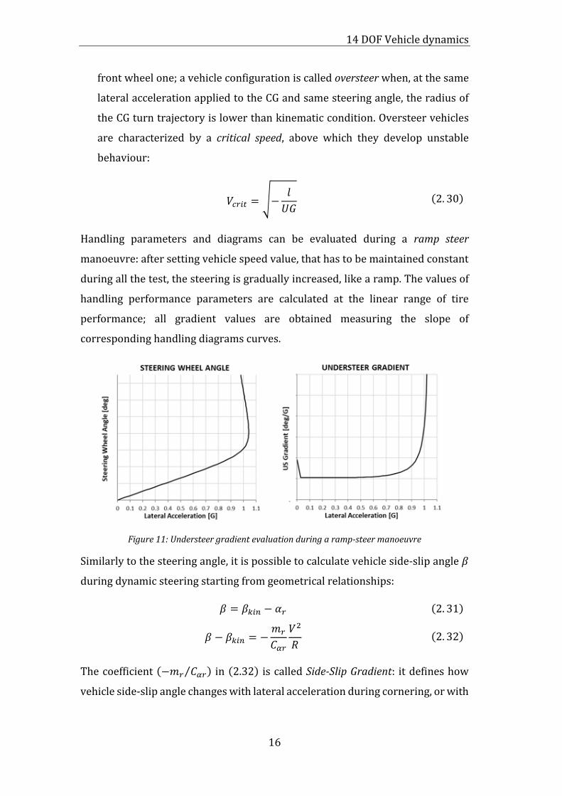
Handling parameters and diagrams can be evaluated during a ramp steer
manoeuvre: after setting vehicle speed value, that has to be maintained constant
during all the test, the steering is gradually increased, like a ramp. The values of
handling performance parameters are calculated at the linear range of tire
performance; all gradient values are obtained measuring the slope of
corresponding handling diagrams curves.
Figure 11: Understeer gradient evaluation during a ramp-steer manoeuvre
Similarly to the steering angle, it is possible to calculate vehicle side-slip angle 𝛽
during dynamic steering starting from geometrical relationships:
𝛽 = 𝛽𝑘𝑖𝑛 − 𝛼𝑟 (2. 31)
𝛽 − 𝛽𝑘𝑖𝑛 = −𝑚𝑟
𝐶𝛼𝑟
𝑉2
𝑅 (2. 32)
The coefficient (−𝑚𝑟 𝐶𝛼𝑟⁄ ) in (2.32) is called Side-Slip Gradient: it defines how
vehicle side-slip angle changes with lateral acceleration during cornering, or with
14 DOF Vehicle dynamics
17
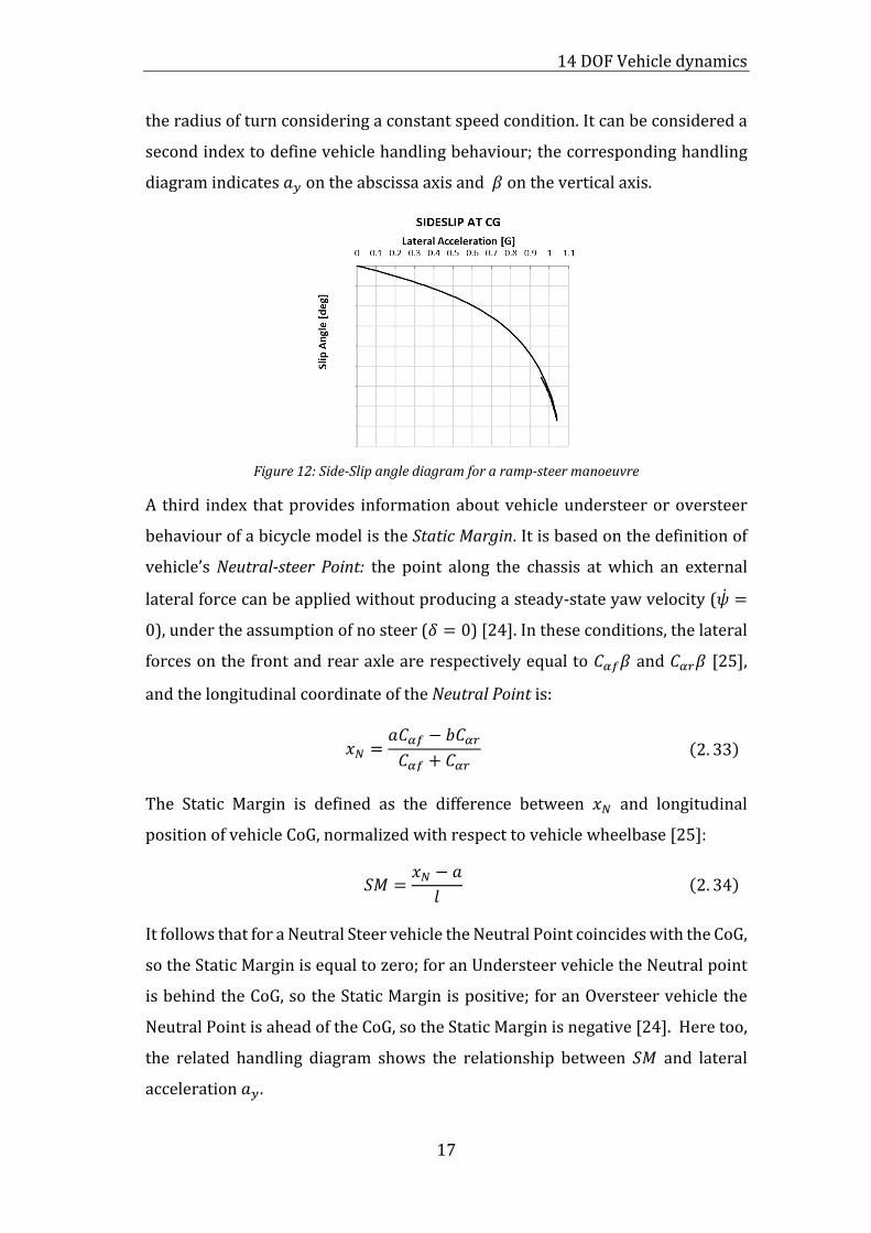
the radius of turn considering a constant speed condition. It can be considered a
second index to define vehicle handling behaviour; the corresponding handling
diagram indicates 𝑎𝑦 on the abscissa axis and 𝛽 on the vertical axis.
Figure 12: Side-Slip angle diagram for a ramp-steer manoeuvre
A third index that provides information about vehicle understeer or oversteer
behaviour of a bicycle model is the Static Margin. It is based on the definition of
vehicle’s Neutral-steer Point: the point along the chassis at which an external
lateral force can be applied without producing a steady-state yaw velocity (�̇� =
0), under the assumption of no steer (𝛿 = 0) [24]. In these conditions, the lateral
forces on the front and rear axle are respectively equal to 𝐶𝛼𝑓𝛽 and 𝐶𝛼𝑟𝛽 [25],
and the longitudinal coordinate of the Neutral Point is:
𝑥𝑁 =𝑎𝐶𝛼𝑓 − 𝑏𝐶𝛼𝑟
𝐶𝛼𝑓 + 𝐶𝛼𝑟 (2. 33)
The Static Margin is defined as the difference between 𝑥𝑁 and longitudinal
position of vehicle CoG, normalized with respect to vehicle wheelbase [25]:
𝑆𝑀 =𝑥𝑁 − 𝑎
𝑙 (2. 34)
It follows that for a Neutral Steer vehicle the Neutral Point coincides with the CoG,
so the Static Margin is equal to zero; for an Understeer vehicle the Neutral point
is behind the CoG, so the Static Margin is positive; for an Oversteer vehicle the
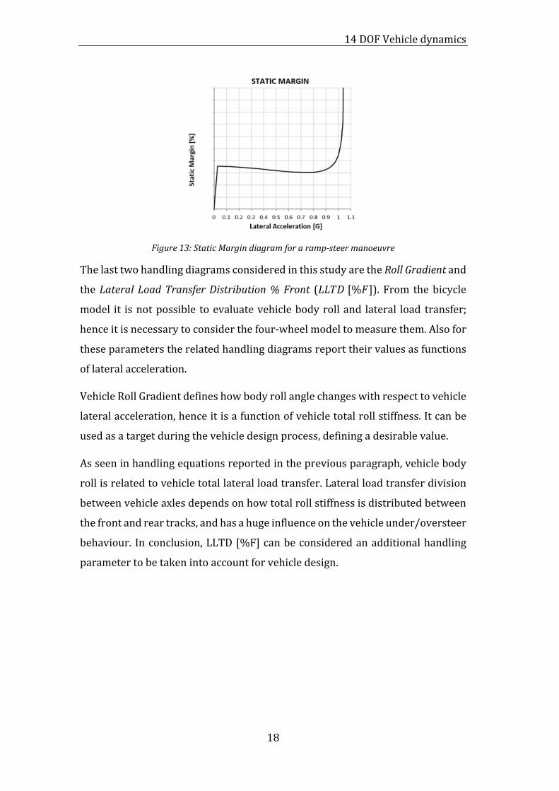
Neutral Point is ahead of the CoG, so the Static Margin is negative [24]. Here too,
the related handling diagram shows the relationship between 𝑆𝑀 and lateral
acceleration 𝑎𝑦.
14 DOF Vehicle dynamics
18
Figure 13: Static Margin diagram for a ramp-steer manoeuvre
The last two handling diagrams considered in this study are the Roll Gradient and
the Lateral Load Transfer Distribution % Front (𝐿𝐿𝑇𝐷 [%𝐹]). From the bicycle
model it is not possible to evaluate vehicle body roll and lateral load transfer;
hence it is necessary to consider the four-wheel model to measure them. Also for
these parameters the related handling diagrams report their values as functions
of lateral acceleration.
Vehicle Roll Gradient defines how body roll angle changes with respect to vehicle
lateral acceleration, hence it is a function of vehicle total roll stiffness. It can be
used as a target during the vehicle design process, defining a desirable value.
As seen in handling equations reported in the previous paragraph, vehicle body
roll is related to vehicle total lateral load transfer. Lateral load transfer division
between vehicle axles depends on how total roll stiffness is distributed between
the front and rear tracks, and has a huge influence on the vehicle under/oversteer
behaviour. In conclusion, LLTD [%F] can be considered an additional handling
parameter to be taken into account for vehicle design.

14 DOF Vehicle dynamics
19
Figure 14: Roll angle and LLTD [%F] diagrams for a ramp-steer manoeuvre
2.4 Tire dynamics
For each wheel, the dynamic equilibrium around its centre is described by (2.35),
where the single degree of freedom is its angular speed:
Figure 15: Wheel free body diagram (adapted from [19])
𝐼𝑊�̇� = 𝑇𝑡𝑟𝑎𝑐𝑡𝑖𝑜𝑛 − 𝑇𝑏𝑟𝑎𝑘𝑒 − 𝐹𝑟𝑒𝑠𝑅𝑙 − 𝐹𝑥𝑅𝑙 (2. 35)
Where:
• 𝐼𝑊 is the wheel inertia;
• 𝑇𝑡𝑟𝑎𝑐𝑡𝑖𝑜𝑛 is the traction torque;
• 𝑇𝑏𝑟𝑎𝑘𝑒 is the brake torque;
• 𝑅𝑙 is the tire loaded radius, calculated as the difference between undeformed
radius and the vertical deflection due to the vertical load on tire (obtained

14 DOF Vehicle dynamics
20
through tire’s vertical stiffness 𝑘𝑣):
𝑅𝑙 = 𝑅𝑤 −𝐹𝑧,𝑡𝑖𝑟𝑒𝑘𝑣
(2. 36)
• 𝐹𝑟𝑒𝑠 is the rolling resistance of the wheel, defined as the product between
wheel’s vertical load on the tire and a rolling coefficient (a polynomial
function of vehicle speed):
𝐹𝑟𝑒𝑠 = (𝑓0 + 𝑓1𝑉 + 𝑓2𝑉4)𝐹𝑧,𝑡𝑖𝑟𝑒 (2. 37)
• 𝐹𝑥 is the longitudinal force transmitted by the tire to the ground; its value
depends on wheel vertical load, friction coefficient with the ground, tire
characteristics and longitudinal deformation during vehicle motion.
Considering a wheel rolling on a level road without applying on it a braking or
tractive torque (pure rolling condition), the rolling radius 𝑅𝑒 , lower than tire
undeformed radius 𝑅𝑤, is defined as the ratio between the longitudinal speed of
the wheel 𝑉 and its angular speed 𝜔0:
𝑅𝑒 =𝑉
𝜔0 (2. 38)
If on the rolling wheel a braking torque is applied, due to tire deformability the
new rolling radius 𝑅′𝑒 is higher than 𝑅𝑒, and the angular velocity 𝜔 lower than
𝜔0; in the same way if a tractive torque is applied on the wheel, 𝑅′𝑒 is lower than
𝑅𝑒, and 𝜔 higher than 𝜔0 [23].
Figure 16: Position of wheel centre of rotation in pure rolling (C), breaking (C') and traction (C'') condition [23]

14 DOF Vehicle dynamics
21
To evaluate the magnitude of tire’s longitudinal deformation, so the difference of
tire condition compared to pure rolling, longitudinal slip 𝑆 is defined:
𝑆 =𝑅𝑒𝜔 − 𝑉
max(𝑉, 𝑅𝑒𝜔) (2. 39)
• during braking, 𝑉 > 𝑅𝑒𝜔, so 0 > 𝑆 > −1
• during traction, 𝑉 < 𝑅𝑒𝜔, so 1 > 𝑆 > 0
The presence of a not negligible longitudinal slip on the tire contact patch
generates a longitudinal wheel ground force.
Figure 17: Curves 𝐹𝑥(𝑆) for different load values for a tire 225/50 R 17 [20]
In the same way, the tire exerts a lateral force when there is a lateral deformation,
detected by the wheel side slip angle (or lateral slip angle) 𝛼:
tan 𝛼 =𝑉𝑐𝑦𝑉𝑐𝑥
(2. 40)
where 𝑉𝑐𝑦 and 𝑉𝑐𝑥 are respectively lateral and longitudinal velocities of the wheel
centre, so by definition 𝛼 is the angle between wheel longitudinal midplane and
wheel velocity direction.
The resultant lateral force 𝐹𝑦 is generally applied at a distance from the centre of
the contact patch, called pneumatic trail 𝑡. As a consequence, it causes a self-
aligning moment 𝑀𝑧 = 𝐹𝑦𝑡 which tends to align the wheel longitudinal midplane
14 DOF Vehicle dynamics
22
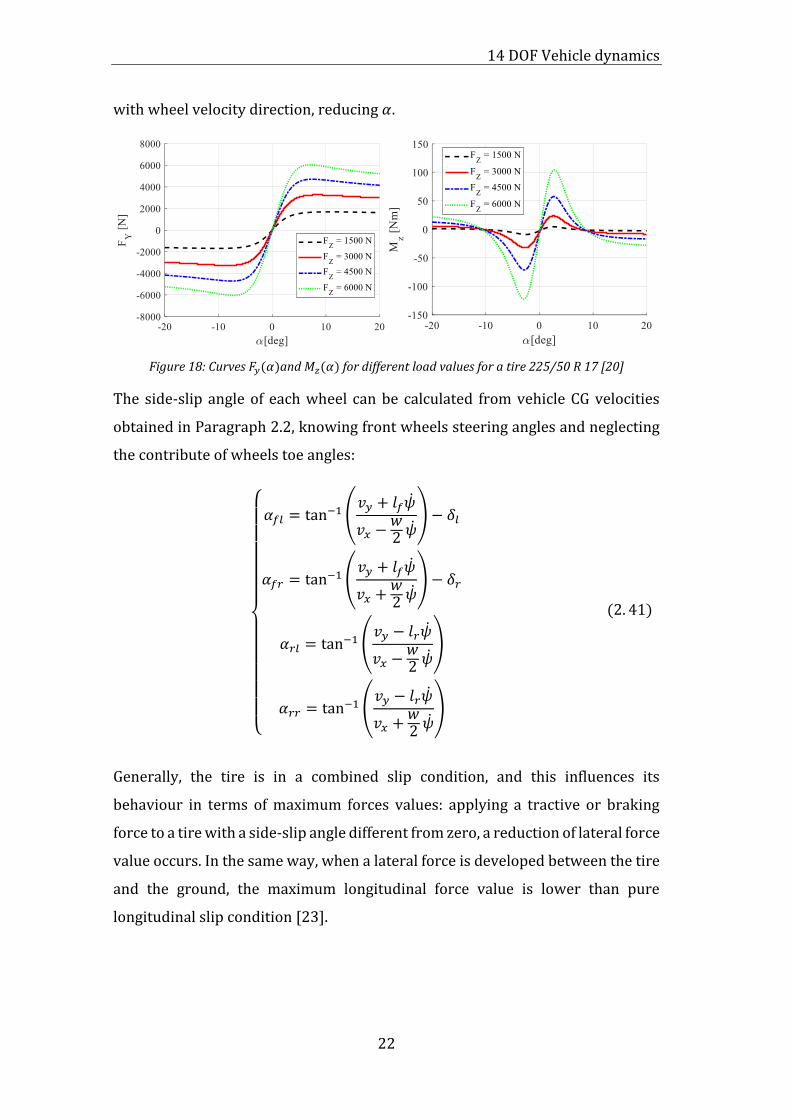
with wheel velocity direction, reducing 𝛼.
Figure 18: Curves 𝐹𝑦(𝛼)and 𝑀𝑧(𝛼) for different load values for a tire 225/50 R 17 [20]
The side-slip angle of each wheel can be calculated from vehicle CG velocities
obtained in Paragraph 2.2, knowing front wheels steering angles and neglecting
the contribute of wheels toe angles:
{
𝛼𝑓𝑙 = tan
−1(𝑣𝑦 + 𝑙𝑓�̇�
𝑣𝑥 −𝑤2�̇�) − 𝛿𝑙
𝛼𝑓𝑟 = tan−1(
𝑣𝑦 + 𝑙𝑓�̇�
𝑣𝑥 +𝑤2�̇�) − 𝛿𝑟
𝛼𝑟𝑙 = tan−1(
𝑣𝑦 − 𝑙𝑟�̇�
𝑣𝑥 −𝑤2 �̇�
)
𝛼𝑟𝑟 = tan−1(
𝑣𝑦 − 𝑙𝑟�̇�
𝑣𝑥 +𝑤2�̇�)
(2. 41)
Generally, the tire is in a combined slip condition, and this influences its
behaviour in terms of maximum forces values: applying a tractive or braking
force to a tire with a side-slip angle different from zero, a reduction of lateral force
value occurs. In the same way, when a lateral force is developed between the tire
and the ground, the maximum longitudinal force value is lower than pure
longitudinal slip condition [23].
14 DOF Vehicle dynamics
23
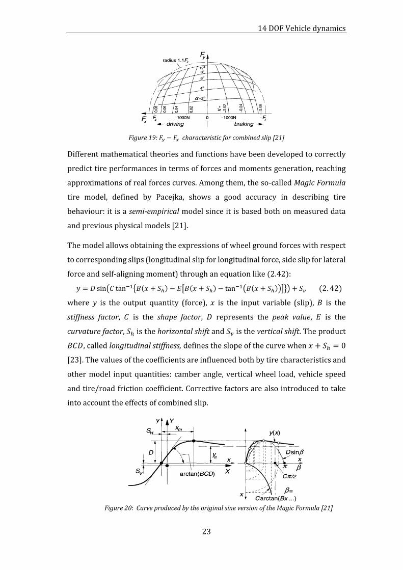
Figure 19: 𝐹𝑦 − 𝐹𝑥 characteristic for combined slip [21]
Different mathematical theories and functions have been developed to correctly
predict tire performances in terms of forces and moments generation, reaching
approximations of real forces curves. Among them, the so-called Magic Formula
tire model, defined by Pacejka, shows a good accuracy in describing tire
behaviour: it is a semi-empirical model since it is based both on measured data
and previous physical models [21].
The model allows obtaining the expressions of wheel ground forces with respect
to corresponding slips (longitudinal slip for longitudinal force, side slip for lateral
force and self-aligning moment) through an equation like (2.42):
𝑦 = 𝐷 sin(𝐶 tan−1{𝐵(𝑥 + 𝑆ℎ) − 𝐸[𝐵(𝑥 + 𝑆ℎ) − tan−1(𝐵(𝑥 + 𝑆ℎ))]}) + 𝑆𝑣 (2. 42)
where 𝑦 is the output quantity (force), 𝑥 is the input variable (slip), 𝐵 is the
stiffness factor, 𝐶 is the shape factor, 𝐷 represents the peak value, 𝐸 is the
curvature factor, 𝑆ℎ is the horizontal shift and 𝑆𝑣 is the vertical shift. The product
𝐵𝐶𝐷, called longitudinal stiffness, defines the slope of the curve when 𝑥 + 𝑆ℎ = 0
[23]. The values of the coefficients are influenced both by tire characteristics and
other model input quantities: camber angle, vertical wheel load, vehicle speed
and tire/road friction coefficient. Corrective factors are also introduced to take
into account the effects of combined slip.
Figure 20: Curve produced by the original sine version of the Magic Formula [21]
24
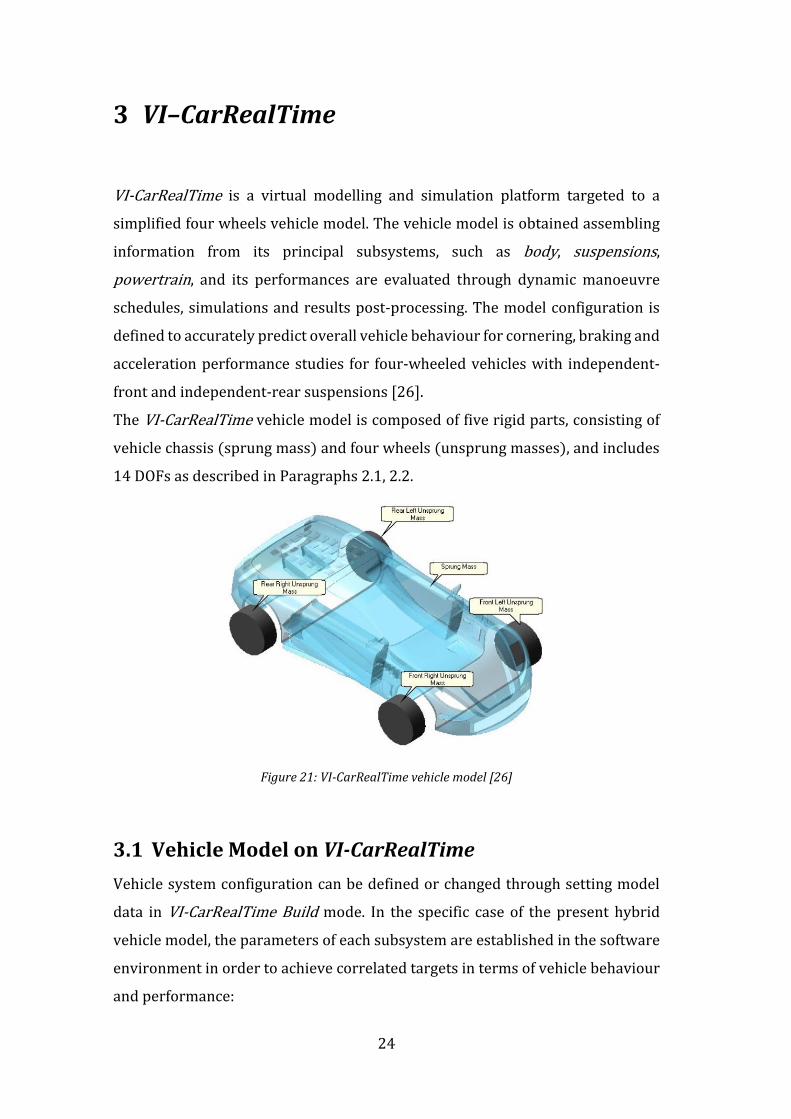
3 VI–CarRealTime
VI-CarRealTime is a virtual modelling and simulation platform targeted to a
simplified four wheels vehicle model. The vehicle model is obtained assembling
information from its principal subsystems, such as body, suspensions,
powertrain, and its performances are evaluated through dynamic manoeuvre
schedules, simulations and results post-processing. The model configuration is
defined to accurately predict overall vehicle behaviour for cornering, braking and
acceleration performance studies for four-wheeled vehicles with independent-
front and independent-rear suspensions [26].
The VI-CarRealTime vehicle model is composed of five rigid parts, consisting of
vehicle chassis (sprung mass) and four wheels (unsprung masses), and includes
14 DOFs as described in Paragraphs 2.1, 2.2.
Figure 21: VI-CarRealTime vehicle model [26]
3.1 Vehicle Model on VI-CarRealTime
Vehicle system configuration can be defined or changed through setting model
data in VI-CarRealTime Build mode. In the specific case of the present hybrid
vehicle model, the parameters of each subsystem are established in the software
environment in order to achieve correlated targets in terms of vehicle behaviour
and performance:

VI–CarRealTime
25
• Body: in this subsystem information about mass, inertia and setup of
vehicle sprung mass can be set. In this case, sprung mass parameters are
defined starting from target specifications about the overall vehicle,
including the presence of the driver, passenger and fuel, and knowing
unsprung masses inertial information:
Vehicle (kerb + 2 passengers + fuel)
Parameter Value
Mass [𝑘𝑔] 1850
Wheelbase [𝑚𝑚] 2600
CoG height [𝑚𝑚] 490
Weigth distribution %Front [%] 48
Rolling inertia 𝐼𝑥𝑥 [𝑘𝑔𝑚2] 700
Pitch inertia 𝐼𝑦𝑦[𝑘𝑔𝑚2] 2600
Yaw inertia 𝐼𝑧𝑧[𝑘𝑔𝑚2] 2900
Table 1: Vehicle parameters
All the vehicle values are defined considering VI-CarRealTime Vehicle
Reference System:
Figure 22: VI-CarRealTime Vehicle Reference System [26]
VI-CarRealTime reference systems are consistent with the standards ISO
8855 and SAE Recommended Practice J670f. As regards Vehicle one, the
origin 𝑆0 is located at 𝑍 = 0 of Global Reference Frame, as shown in Figure
22, and at half front vehicle track. The axes are oriented, at design time,
with 𝑋 + pointing forward in the direction of motion, 𝑌 + pointing
leftward, 𝑍 + pointing upward [26].
VI–CarRealTime
26
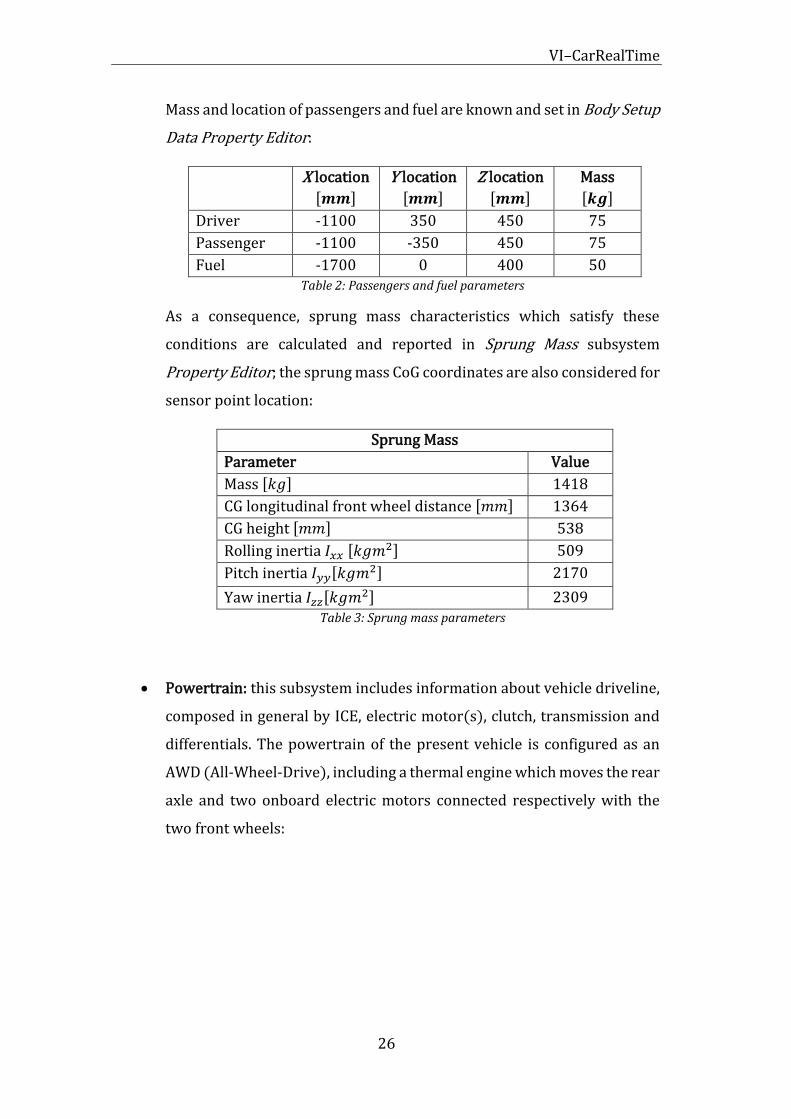
Mass and location of passengers and fuel are known and set in Body Setup
Data Property Editor:
X location
[𝒎𝒎]
Y location
[𝒎𝒎]
Z location
[𝒎𝒎]
Mass
[𝒌𝒈]
Driver -1100 350 450 75
Passenger -1100 -350 450 75
Fuel -1700 0 400 50 Table 2: Passengers and fuel parameters
As a consequence, sprung mass characteristics which satisfy these
conditions are calculated and reported in Sprung Mass subsystem
Property Editor; the sprung mass CoG coordinates are also considered for
sensor point location:
Sprung Mass
Parameter Value
Mass [𝑘𝑔] 1418
CG longitudinal front wheel distance [𝑚𝑚] 1364
CG height [𝑚𝑚] 538
Rolling inertia 𝐼𝑥𝑥 [𝑘𝑔𝑚2] 509
Pitch inertia 𝐼𝑦𝑦[𝑘𝑔𝑚2] 2170
Yaw inertia 𝐼𝑧𝑧[𝑘𝑔𝑚2] 2309
Table 3: Sprung mass parameters
• Powertrain: this subsystem includes information about vehicle driveline,
composed in general by ICE, electric motor(s), clutch, transmission and
differentials. The powertrain of the present vehicle is configured as an
AWD (All-Wheel-Drive), including a thermal engine which moves the rear
axle and two onboard electric motors connected respectively with the
two front wheels:
VI–CarRealTime
27
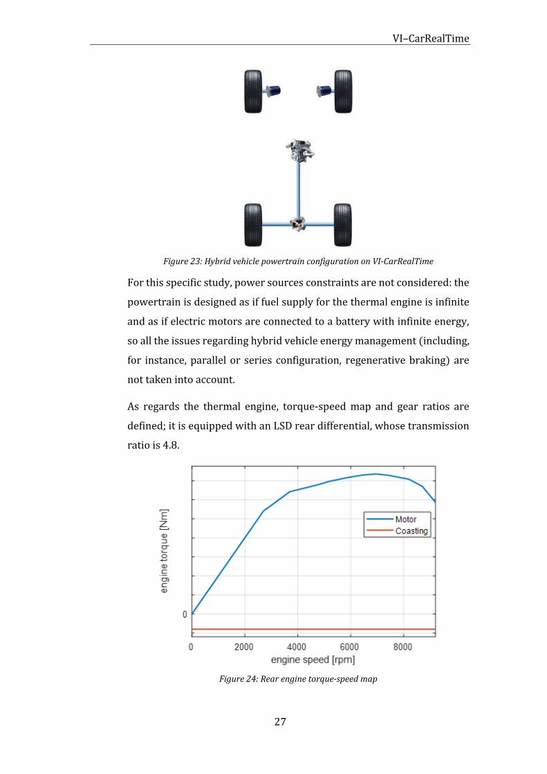
Figure 23: Hybrid vehicle powertrain configuration on VI-CarRealTime
For this specific study, power sources constraints are not considered: the
powertrain is designed as if fuel supply for the thermal engine is infinite
and as if electric motors are connected to a battery with infinite energy,
so all the issues regarding hybrid vehicle energy management (including,
for instance, parallel or series configuration, regenerative braking) are
not taken into account.
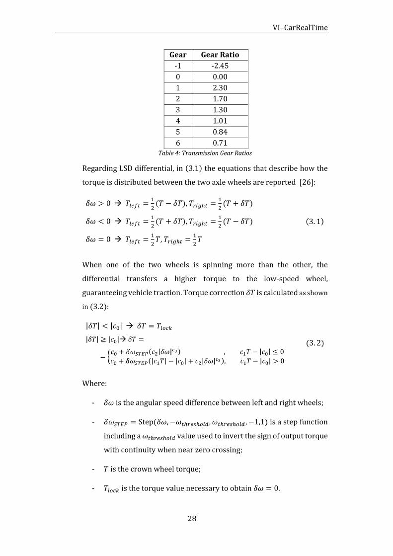
As regards the thermal engine, torque-speed map and gear ratios are
defined; it is equipped with an LSD rear differential, whose transmission
ratio is 4.8.
Figure 24: Rear engine torque-speed map
VI–CarRealTime
28
Gear Gear Ratio
-1 -2.45
0 0.00
1 2.30
2 1.70
3 1.30
4 1.01
5 0.84
6 0.71 Table 4: Transmission Gear Ratios
Regarding LSD differential, in (3.1) the equations that describe how the
torque is distributed between the two axle wheels are reported [26]:
𝛿𝜔 > 0 → 𝑇𝑙𝑒𝑓𝑡 =1
2(𝑇 − 𝛿𝑇), 𝑇𝑟𝑖𝑔ℎ𝑡 =
1
2(𝑇 + 𝛿𝑇)
𝛿𝜔 < 0 → 𝑇𝑙𝑒𝑓𝑡 =1
2(𝑇 + 𝛿𝑇), 𝑇𝑟𝑖𝑔ℎ𝑡 =
1
2(𝑇 − 𝛿𝑇)
𝛿𝜔 = 0 → 𝑇𝑙𝑒𝑓𝑡 =1
2𝑇, 𝑇𝑟𝑖𝑔ℎ𝑡 =
1
2𝑇
(3. 1)
When one of the two wheels is spinning more than the other, the
differential transfers a higher torque to the low-speed wheel,
guaranteeing vehicle traction. Torque correction 𝛿𝑇 is calculated as shown
in (3.2):
|𝛿𝑇| < |𝑐0| → 𝛿𝑇 = 𝑇𝑙𝑜𝑐𝑘
|𝛿𝑇| ≥ |𝑐0|→ 𝛿𝑇 =
= {𝑐0 + 𝛿𝜔𝑆𝑇𝐸𝑃(𝑐2|𝛿𝜔|
𝑐3) , 𝑐1𝑇 − |𝑐0| ≤ 0
𝑐0 + 𝛿𝜔𝑆𝑇𝐸𝑃(|𝑐1𝑇| − |𝑐0| + 𝑐2|𝛿𝜔|𝑐3), 𝑐1𝑇 − |𝑐0| > 0
(3. 2)
Where:
- 𝛿𝜔 is the angular speed difference between left and right wheels;
- 𝛿𝜔𝑆𝑇𝐸𝑃 = Step(𝛿𝜔,−𝜔𝑡ℎ𝑟𝑒𝑠ℎ𝑜𝑙𝑑, 𝜔𝑡ℎ𝑟𝑒𝑠ℎ𝑜𝑙𝑑, −1,1) is a step function
including a 𝜔𝑡ℎ𝑟𝑒𝑠ℎ𝑜𝑙𝑑 value used to invert the sign of output torque
with continuity when near zero crossing;
- 𝑇 is the crown wheel torque;
- 𝑇𝑙𝑜𝑐𝑘 is the torque value necessary to obtain 𝛿𝜔 = 0.
VI–CarRealTime
29
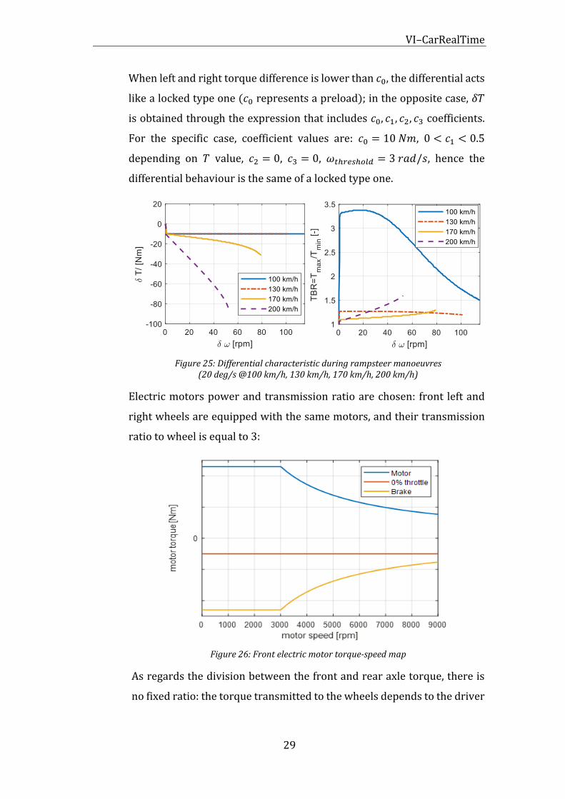
When left and right torque difference is lower than 𝑐0, the differential acts
like a locked type one (𝑐0 represents a preload); in the opposite case, 𝛿𝑇
is obtained through the expression that includes 𝑐0, 𝑐1, 𝑐2, 𝑐3 coefficients.
For the specific case, coefficient values are: 𝑐0 = 10 𝑁𝑚, 0 < 𝑐1 < 0.5
depending on 𝑇 value, 𝑐2 = 0, 𝑐3 = 0, 𝜔𝑡ℎ𝑟𝑒𝑠ℎ𝑜𝑙𝑑 = 3 𝑟𝑎𝑑/𝑠, hence the
differential behaviour is the same of a locked type one.
Figure 25: Differential characteristic during rampsteer manoeuvres (20 deg/s @100 km/h, 130 km/h, 170 km/h, 200 km/h)
Electric motors power and transmission ratio are chosen: front left and
right wheels are equipped with the same motors, and their transmission
ratio to wheel is equal to 3:
Figure 26: Front electric motor torque-speed map
As regards the division between the front and rear axle torque, there is
no fixed ratio: the torque transmitted to the wheels depends to the driver
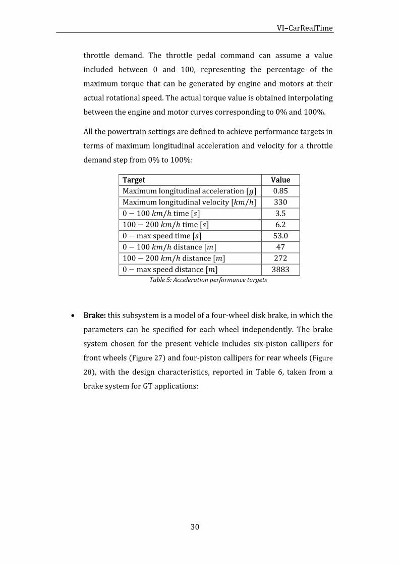
VI–CarRealTime
30
throttle demand. The throttle pedal command can assume a value
included between 0 and 100, representing the percentage of the
maximum torque that can be generated by engine and motors at their
actual rotational speed. The actual torque value is obtained interpolating
between the engine and motor curves corresponding to 0% and 100%.
All the powertrain settings are defined to achieve performance targets in
terms of maximum longitudinal acceleration and velocity for a throttle
demand step from 0% to 100%:
Target Value
Maximum longitudinal acceleration [𝑔] 0.85
Maximum longitudinal velocity [𝑘𝑚/ℎ] 330
0 − 100 𝑘𝑚/ℎ time [𝑠] 3.5
100 − 200 𝑘𝑚/ℎ time [𝑠] 6.2
0 − max speed time [𝑠] 53.0
0 − 100 𝑘𝑚/ℎ distance [𝑚] 47
100 − 200 𝑘𝑚/ℎ distance [𝑚] 272
0 − max speed distance [𝑚] 3883 Table 5: Acceleration performance targets
• Brake: this subsystem is a model of a four-wheel disk brake, in which the
parameters can be specified for each wheel independently. The brake
system chosen for the present vehicle includes six-piston callipers for
front wheels (Figure 27) and four-piston callipers for rear wheels (Figure
28), with the design characteristics, reported in Table 6, taken from a
brake system for GT applications:

VI–CarRealTime
31
Element Front value
(left and right)
Rear value
(left and right)
Brake pedal ratio [%] 50 50
Master cylinder diameter [𝑚𝑚] 30 30
Calliper acting radius diameter [𝑚𝑚] 152.5 140
Calliper piston 1 diameter [𝑚𝑚] 38 36
Calliper piston 2 diameter [𝑚𝑚] 30 28
Calliper piston 3 diameter [𝑚𝑚] 28 36
Calliper piston 4 diameter [𝑚𝑚] 38 28
Calliper piston 5 diameter [𝑚𝑚] 30 -
Calliper piston 6 diameter [𝑚𝑚] 28 -
Pad friction coefficient [−] 0.43 0.47 Table 6: Brake system characteristics
Figure 27: Front brake calliper [27]
Figure 28: Rear brake calliper [27]
This brake configuration permits to obtain a brake torque distribution
front of 60 % and to reach a target maximum longitudinal acceleration of
1.2 𝑔 in a 100 − 0 𝑘𝑚/ℎ breaking manoeuvre.
• Front and rear suspensions: in VI-CarRealTime, suspensions subsystems
are described using a conceptual approach: there are no physical part or
linkage in the model, but lookup tables describe the suspensions’

VI–CarRealTime
32
behaviour, so computational times are reduced.
The movement of the wheel is related to vertical jounce (independent
variable in equations of motion) through a proper constraint in order to
define wheel position and orientation (remaining wheel 5 DOFs) by
lookup tables. Suspensions kinematic can be modelled as independent, as
a function of corresponding single wheel jounce, or dependent, as a
function of both left and right wheels jounces. The compliance effect is
taken into account considering wheel position and orientation as
functions of wheel jounce and external load. The effect of suspension
components (springs, dampers, bumpers) is projected onto wheels:
lookup tables are used to get element forces applied at the respective
component, and a motion ratio from wheel to suspension component
travel is exploited to obtain equivalent force at wheel centre [26].
Figure 29: VI-CarRealTime suspension forces evaluation [26]
As regards the vehicle object of this study, the suspensions specifications
are modelled importing some K&C results for subsystem lookup tables
and defining the components parameters shown in Table 7 and Figure 31:

VI–CarRealTime
33
Wheel location
Front Rear
Track [𝑚𝑚] 1680 1650
Springs
Front Rear
Preload [𝑁] 6170 5550
Stiffness [𝑁/𝑚𝑚] 85 80
Anti-Roll Bar
Front Rear
Stiffness (SWT)[𝑁/𝑚𝑚] 26.3 17.5
Bumpers
Front Rear
Bumpstop clearance [𝑚𝑚] 15.5 26.9
Reboundstop clearance [𝑚𝑚] 55 63
Static wheel angles
Front Rear
Toe [𝑑𝑒𝑔] -0.1 0.15
Camber [𝑑𝑒𝑔] -1 -1.5 Table 7: Front and rear suspension characteristics
Figure 30: Toe and Camber angles VI-CarRealTime sign reference
Figure 31: Dampers’ characteristics
VI–CarRealTime
34
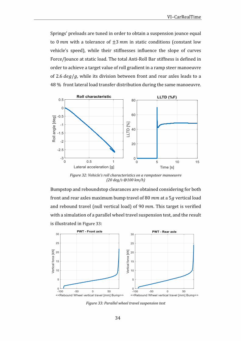
Springs’ preloads are tuned in order to obtain a suspension jounce equal
to 0 𝑚𝑚 with a tolerance of ±3 𝑚𝑚 in static conditions (constant low
vehicle’s speed), while their stiffnesses influence the slope of curves
Force/Jounce at static load. The total Anti-Roll Bar stiffness is defined in
order to achieve a target value of roll gradient in a ramp steer manoeuvre
of 2.6 𝑑𝑒𝑔/𝑔, while its division between front and rear axles leads to a
48 % front lateral load transfer distribution during the same manoeuvre.
Figure 32: Vehicle’s roll characteristics on a rampsteer manoeuvre (20 deg/s @100 km/h)
Bumpstop and reboundstop clearances are obtained considering for both
front and rear axles maximum bump travel of 80 𝑚𝑚 at a 5𝑔 vertical load
and rebound travel (null vertical load) of 90 𝑚𝑚. This target is verified
with a simulation of a parallel wheel travel suspension test, and the result
is illustrated in Figure 33:
Figure 33: Parallel wheel travel suspension test

VI–CarRealTime
35
• Front and rear unsprung masses and tires: these subsystems collect
information about mass and inertia of unsprung mass pairs of the vehicle
model; they also acquire information about tires’ behaviour through tire
property files, which include tires characteristics defined through
coefficients of Pacejka tire model.
In tire property files used for this vehicle, some coefficients, in particular
the scaling coefficients 𝜆 of Pacejka formulas, are tuned in order to
achieve target handling performances (evaluated in a ramp steer
manoeuvre): acting on cornering stiffnesses of front and rear tires, an
understeer gradient of 56 𝑑𝑒𝑔/𝑔 and a sideslip gradient of 0.81 𝑑𝑒𝑔/𝑔
are reached.
Figure 34: Vehicle’s handling characteristics on a rampsteer manoeuvre (20 deg/s @100 km/h)
Figure 35: Vehicle's static margin

VI–CarRealTime
36
3.2 Co-simulation with MATLAB/Simulink
Through a specific interface, VI-CarRealTime environment can interact with
MATLAB/Simulink: it is possible to connect the vehicle model with MATLAB and
use MATLAB tools to make it more complicated, adding for example control
systems or accessories developed in MATLAB/Simulink itself. This interface
allows the user to run co-simulations and analyse test results.
The VI-CarRealTime model is shared with the MATLAB environment as an s-
function representing the car plant; the s-function receives the car data from VI-
CarRealTime as a parameter consisting of a file which collects all the model
information. Some input and output ports can be specified at the s-function,
choosing them from lists of possible channels, so the resulting overall interface is
a unique Simulink block that can be connected to other blocks through its ports.
Figure 36: VI-CarRealTime model Simulink block (s-function)
Figure 37: Simulink interface for VI-CarRealTime s-function input ports
VI–CarRealTime
37
To start a co-simulation, the user has first to follow the standard approach on the
VI-CarRealTime platform as if he has to run a standalone simulation, setting the
vehicle model and the manoeuvre event. After making the set-up actions useful
to make MATLAB s-function communicate with the defined VI-CarRealTime event,
it is possible to run the co-simulation from the Simulink environment.
38
4 Traction Control System
4.1 Traction Control action
As already mentioned, Traction Control System (TCS) objective is to limit driving
wheels longitudinal slip under a threshold value in order to prevent wheels
spinning during accelerations, especially with low friction surface road; the
control also aims to maintain wheel slip near the optimal value, which
corresponds to maximum possible longitudinal wheel ground force [28].
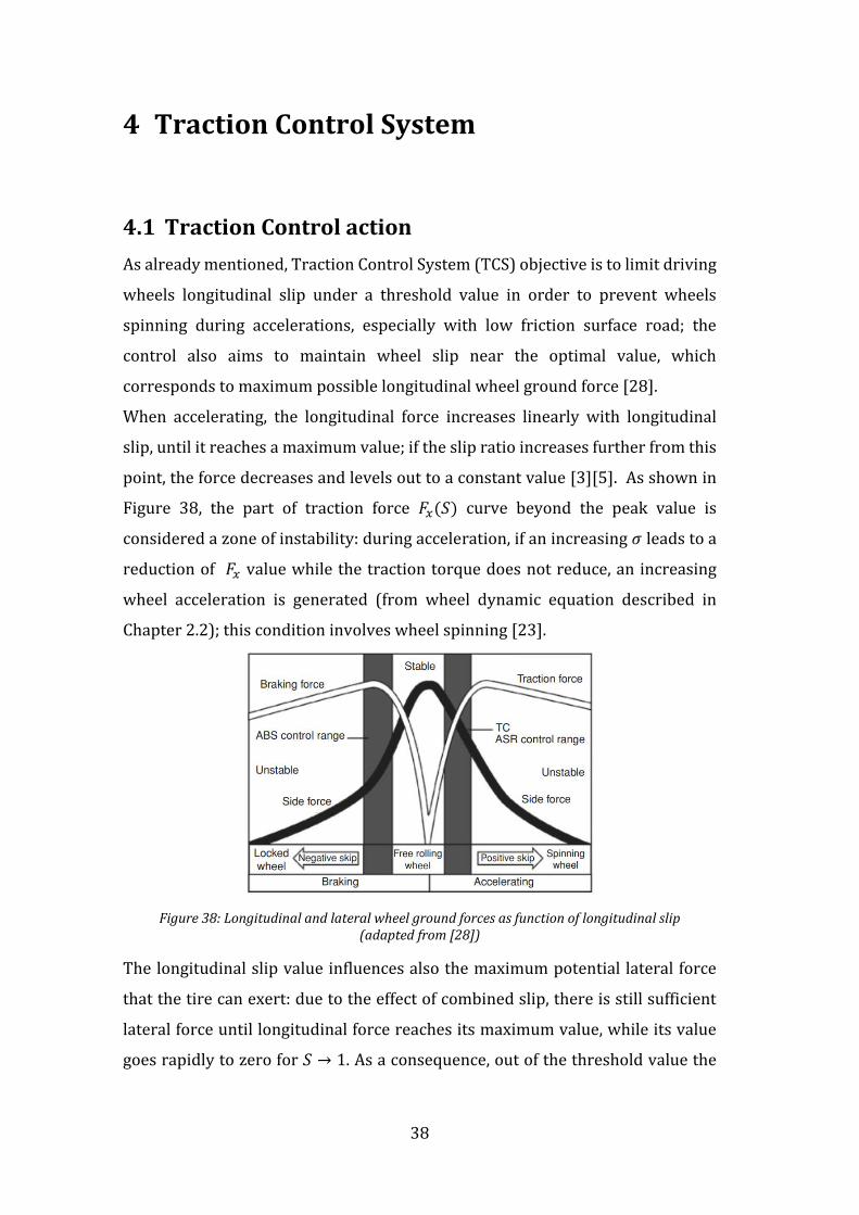
When accelerating, the longitudinal force increases linearly with longitudinal
slip, until it reaches a maximum value; if the slip ratio increases further from this
point, the force decreases and levels out to a constant value [3][5]. As shown in
Figure 38, the part of traction force 𝐹𝑥(𝑆) curve beyond the peak value is
considered a zone of instability: during acceleration, if an increasing 𝜎 leads to a
reduction of 𝐹𝑥 value while the traction torque does not reduce, an increasing
wheel acceleration is generated (from wheel dynamic equation described in
Chapter 2.2); this condition involves wheel spinning [23].
Figure 38: Longitudinal and lateral wheel ground forces as function of longitudinal slip (adapted from [28])
The longitudinal slip value influences also the maximum potential lateral force
that the tire can exert: due to the effect of combined slip, there is still sufficient
lateral force until longitudinal force reaches its maximum value, while its value
goes rapidly to zero for 𝑆 → 1. As a consequence, out of the threshold value the

Traction Control System
39
vehicle stability is compromised because its force capacity in the lateral direction
is severely reduced: spinning front or rear wheels lead respectively to the loss of
steering control or directional stability [28]. In this case, an incorrect reaction of
the driver causes the loss of vehicle control, in particular on slippery roads or at
turns [8].
TCS purpose of keeping the wheel inside the stable slip range is basically obtained
with limiting the driving power to the wheel. A proper control has to be precise,
dynamic, capable to detect and react to changes of condition in real-time, and
robust with respect to external disturbances [30].
The limiting action of TCS maximizes vehicle’s longitudinal acceleration both in
straight lines and cornering since it enhances the longitudinal performance of
driving tires without exceeding their limits [30]. At the same time, it ensures
handling stability, guaranteeing satisfactory tire performance in the lateral
direction, and so vehicle safety.
4.2 Traction Control Design
The vehicle object of this study presents three different driving modes that can
be directly selected by the driver with a switch, depending on environmental
conditions and personal driving preferences:
• Comfort: it represents the default mode, used for routine drives; the vehicle
offers a “middle” performance, balanced between powertrain efficiency and
comfort drive feel;
• Wet: used in case of rain or adverse conditions in general, when the driver
realizes the vehicle shows less traction compared to dry roads; it supports the
driver when driving on a slippery road surface, helping him to maintain
vehicle stability;
• Sport: used on track to reach the maximum of vehicle’s dynamic
performances, makes the most of the powertrain possibilities.
It follows that the TCS algorithm settings have to be adjusted in order to adapt its
operations to the whole vehicle mode performance. In Comfort mode, the control
operation has to ensure vehicle stability considering generally dry condition
Traction Control System
40
roads. In Wet mode the control has to guarantee safety, being more reactive when
wheels lose the grip on low-friction roads and limiting the tractive power quickly
and much more than Comfort mode. In Sport mode, the control has to let the
vehicle enhance its longitudinal and lateral handling, so its action has to be
smoother than Comfort mode.
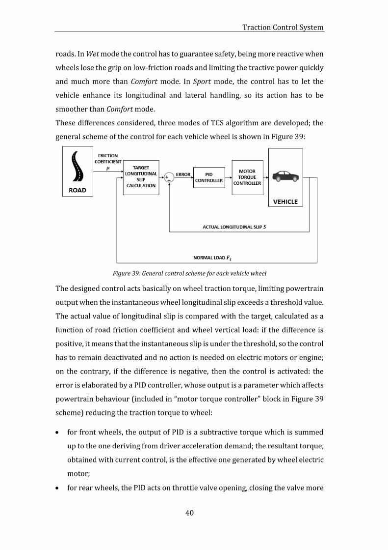
These differences considered, three modes of TCS algorithm are developed; the
general scheme of the control for each vehicle wheel is shown in Figure 39:
Figure 39: General control scheme for each vehicle wheel
The designed control acts basically on wheel traction torque, limiting powertrain
output when the instantaneous wheel longitudinal slip exceeds a threshold value.
The actual value of longitudinal slip is compared with the target, calculated as a
function of road friction coefficient and wheel vertical load: if the difference is
positive, it means that the instantaneous slip is under the threshold, so the control
has to remain deactivated and no action is needed on electric motors or engine;
on the contrary, if the difference is negative, then the control is activated: the
error is elaborated by a PID controller, whose output is a parameter which affects
powertrain behaviour (included in “motor torque controller” block in Figure 39
scheme) reducing the traction torque to wheel:
• for front wheels, the output of PID is a subtractive torque which is summed
up to the one deriving from driver acceleration demand; the resultant torque,
obtained with current control, is the effective one generated by wheel electric
motor;
• for rear wheels, the PID acts on throttle valve opening, closing the valve more

Traction Control System
41
than it would be expected from driver acceleration command; in this way, the
engine output torque would be lower.
It follows that front wheels can be controlled independently, because each of
them is connected to the corresponding electric motor; as a consequence, on front
wheels it is possible to optimize longitudinal slip control.
As regards rear wheels, both of them are moved by the engine, thus it is necessary
to define which wheel has to be taken as reference for the activation of the
control. It also follows that control action itself would not always optimize the
slip condition of both the two wheels. In particular, when rear wheels are
travelling simultaneously on different friction surfaces: if the control activates
referring to the wheel which is spinning more, it will slow down also the wheel
that has not yet exceeded the slip limit, penalizing rear axle traction; if the control
considers less spinning wheel as the target of activation, it will allow the other
wheel to reach high longitudinal slip value, reducing vehicle stability with respect
to the previous situation. Based on specific targets of each driving mode, it would
be more proper to choose the first or second case.
To avoid the possibility that the control turns repeatedly ON and OFF when the
actual longitudinal slip value is around the target one, a hysteresis algorithm is
implemented: ON and OFF thresholds have different values and limit a neutral
zone that includes the target slip; the control activates when the monitored slip
is higher than the upper value and deactivates when it is under the lower one.
4.2.1 Target longitudinal slip calculation
The target longitudinal slip is the value that has to be compared with the
instantaneous slip one to determine traction control activation.
As explained in Paragraph 4.1, the wheel longitudinal slip has to remain under
the value for which maximum longitudinal force is generated. Considering to be
in pure longitudinal slip condition, wheel’s ground longitudinal force depends, as
well as on longitudinal slip, on wheel’s vertical load 𝐹𝑧 and road friction
coefficient 𝜇. For this study the Pacejka tire model is considered, for which
Traction Control System
42
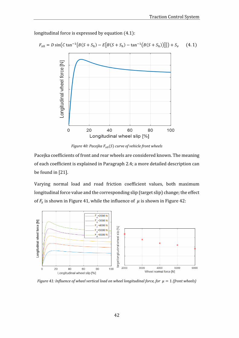
longitudinal force is expressed by equation (4.1):
𝐹𝑥0 = 𝐷 sin(𝐶 tan−1{𝐵(𝑆 + 𝑆ℎ) − 𝐸[𝐵(𝑆 + 𝑆ℎ) − tan
−1(𝐵(𝑆 + 𝑆ℎ))]}) + 𝑆𝑣 (4. 1)
Figure 40: Pacejka 𝐹𝑥0(𝑆) curve of vehicle front wheels
Pacejka coefficients of front and rear wheels are considered known. The meaning
of each coefficient is explained in Paragraph 2.4; a more detailed description can
be found in [21].
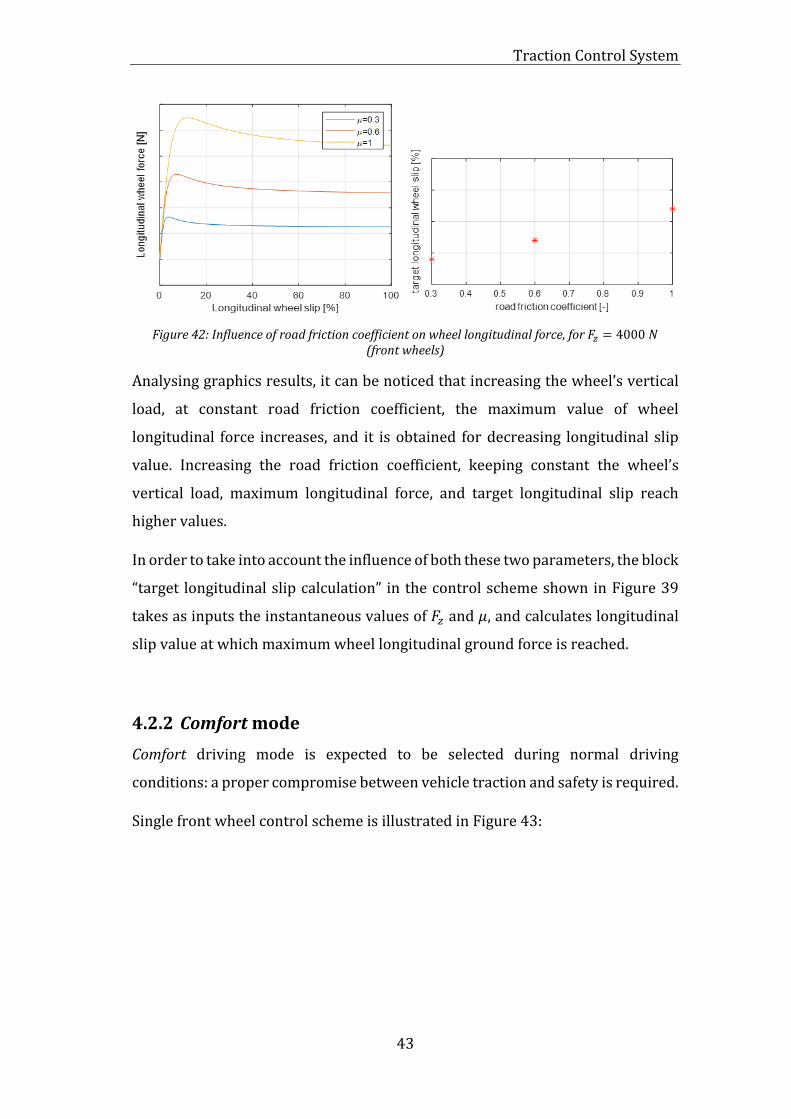
Varying normal load and road friction coefficient values, both maximum
longitudinal force value and the corresponding slip (target slip) change; the effect
of 𝐹𝑧 is shown in Figure 41, while the influence of 𝜇 is shown in Figure 42:
Figure 41: Influence of wheel vertical load on wheel longitudinal force, for 𝜇 = 1 (front wheels)
Traction Control System
43
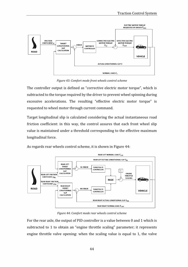
Figure 42: Influence of road friction coefficient on wheel longitudinal force, for 𝐹𝑧 = 4000 𝑁 (front wheels)
Analysing graphics results, it can be noticed that increasing the wheel’s vertical
load, at constant road friction coefficient, the maximum value of wheel
longitudinal force increases, and it is obtained for decreasing longitudinal slip
value. Increasing the road friction coefficient, keeping constant the wheel’s
vertical load, maximum longitudinal force, and target longitudinal slip reach
higher values.
In order to take into account the influence of both these two parameters, the block
“target longitudinal slip calculation” in the control scheme shown in Figure 39
takes as inputs the instantaneous values of 𝐹𝑧 and 𝜇, and calculates longitudinal
slip value at which maximum wheel longitudinal ground force is reached.
4.2.2 Comfort mode
Comfort driving mode is expected to be selected during normal driving
conditions: a proper compromise between vehicle traction and safety is required.
Single front wheel control scheme is illustrated in Figure 43:
Traction Control System
44
Figure 43: Comfort mode front wheels control scheme
The controller output is defined as “corrective electric motor torque”, which is
subtracted to the torque required by the driver to prevent wheel spinning during
excessive accelerations. The resulting “effective electric motor torque” is
requested to wheel motor through current command.
Target longitudinal slip is calculated considering the actual instantaneous road
friction coefficient: in this way, the control assures that each front wheel slip
value is maintained under a threshold corresponding to the effective maximum
longitudinal force.
As regards rear wheels control scheme, it is shown in Figure 44:
Figure 44: Comfort mode rear wheels control scheme
For the rear axle, the output of PID controller is a value between 0 and 1 which is
subtracted to 1 to obtain an “engine throttle scaling” parameter; it represents
engine throttle valve opening: when the scaling value is equal to 1, the valve
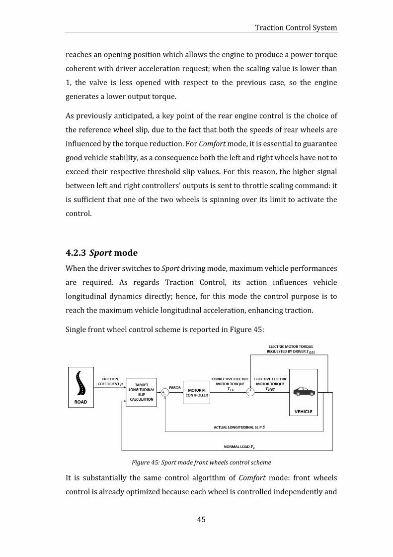
Traction Control System
45
reaches an opening position which allows the engine to produce a power torque
coherent with driver acceleration request; when the scaling value is lower than
1, the valve is less opened with respect to the previous case, so the engine
generates a lower output torque.
As previously anticipated, a key point of the rear engine control is the choice of
the reference wheel slip, due to the fact that both the speeds of rear wheels are
influenced by the torque reduction. For Comfort mode, it is essential to guarantee
good vehicle stability, as a consequence both the left and right wheels have not to
exceed their respective threshold slip values. For this reason, the higher signal
between left and right controllers’ outputs is sent to throttle scaling command: it
is sufficient that one of the two wheels is spinning over its limit to activate the
control.
4.2.3 Sport mode
When the driver switches to Sport driving mode, maximum vehicle performances
are required. As regards Traction Control, its action influences vehicle
longitudinal dynamics directly; hence, for this mode the control purpose is to
reach the maximum vehicle longitudinal acceleration, enhancing traction.
Single front wheel control scheme is reported in Figure 45:
Figure 45: Sport mode front wheels control scheme
It is substantially the same control algorithm of Comfort mode: front wheels
control is already optimized because each wheel is controlled independently and
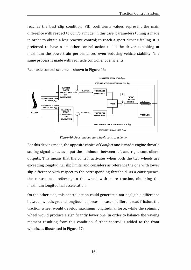
Traction Control System
46
reaches the best slip condition. PID coefficients values represent the main
difference with respect to Comfort mode: in this case, parameters tuning is made
in order to obtain a less reactive control; to reach a sport driving feeling, it is
preferred to have a smoother control action to let the driver exploiting at
maximum the powertrain performances, even reducing vehicle stability. The
same process is made with rear axle controller coefficients.
Rear axle control scheme is shown in Figure 46:
Figure 46: Sport mode rear wheels control scheme
For this driving mode, the opposite choice of Comfort one is made: engine throttle
scaling signal takes as input the minimum between left and right controllers’
outputs. This means that the control activates when both the two wheels are
exceeding longitudinal slip limits, and considers as reference the one with lower
slip difference with respect to the corresponding threshold. As a consequence,
the control acts referring to the wheel with more traction, obtaining the
maximum longitudinal acceleration.
On the other side, this control action could generate a not negligible difference
between wheels ground longitudinal forces: in case of different road friction, the
traction wheel would develop maximum longitudinal force, while the spinning
wheel would produce a significantly lower one. In order to balance the yawing
moment resulting from this condition, further control is added to the front
wheels, as illustrated in Figure 47:
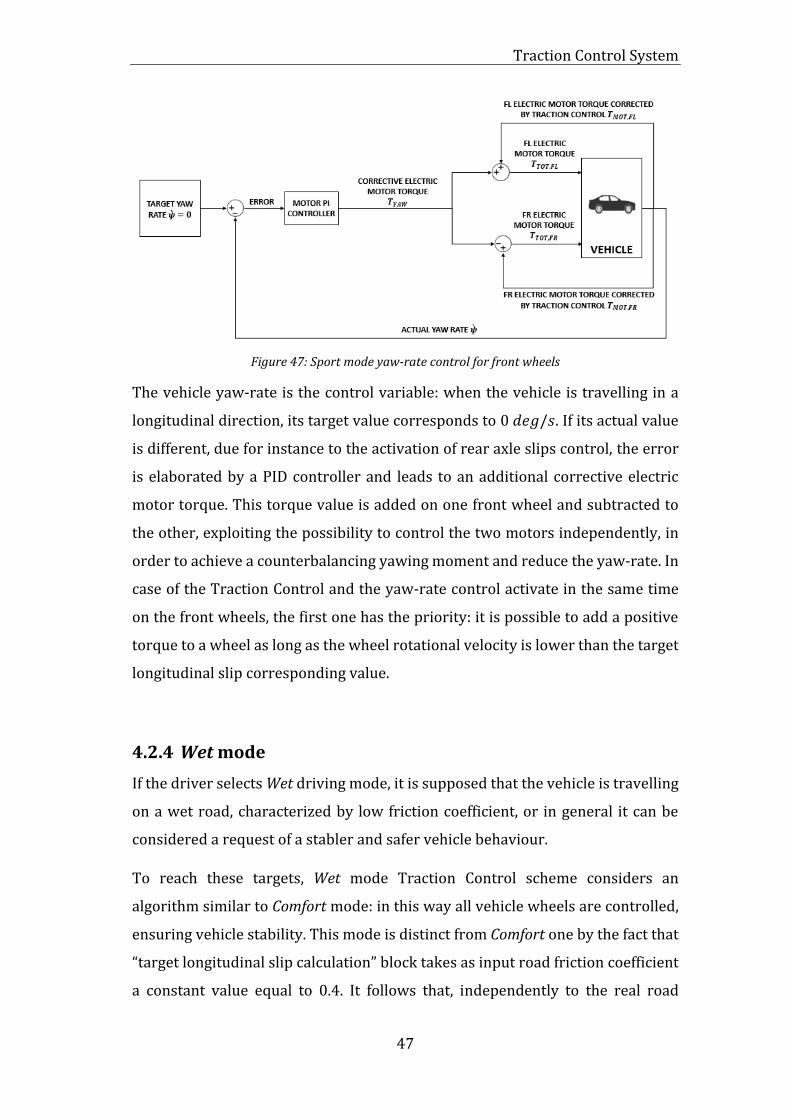
Traction Control System
47
Figure 47: Sport mode yaw-rate control for front wheels
The vehicle yaw-rate is the control variable: when the vehicle is travelling in a
longitudinal direction, its target value corresponds to 0 𝑑𝑒𝑔/𝑠. If its actual value
is different, due for instance to the activation of rear axle slips control, the error
is elaborated by a PID controller and leads to an additional corrective electric
motor torque. This torque value is added on one front wheel and subtracted to
the other, exploiting the possibility to control the two motors independently, in
order to achieve a counterbalancing yawing moment and reduce the yaw-rate. In
case of the Traction Control and the yaw-rate control activate in the same time
on the front wheels, the first one has the priority: it is possible to add a positive
torque to a wheel as long as the wheel rotational velocity is lower than the target
longitudinal slip corresponding value.
4.2.4 Wet mode
If the driver selects Wet driving mode, it is supposed that the vehicle is travelling
on a wet road, characterized by low friction coefficient, or in general it can be
considered a request of a stabler and safer vehicle behaviour.
To reach these targets, Wet mode Traction Control scheme considers an
algorithm similar to Comfort mode: in this way all vehicle wheels are controlled,
ensuring vehicle stability. This mode is distinct from Comfort one by the fact that
“target longitudinal slip calculation” block takes as input road friction coefficient
a constant value equal to 0.4. It follows that, independently to the real road
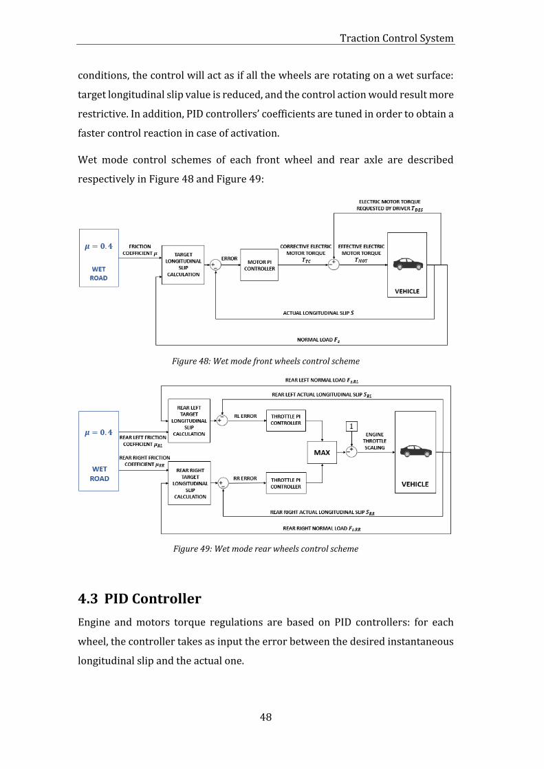
Traction Control System
48
conditions, the control will act as if all the wheels are rotating on a wet surface:
target longitudinal slip value is reduced, and the control action would result more
restrictive. In addition, PID controllers’ coefficients are tuned in order to obtain a
faster control reaction in case of activation.
Wet mode control schemes of each front wheel and rear axle are described
respectively in Figure 48 and Figure 49:
Figure 48: Wet mode front wheels control scheme
Figure 49: Wet mode rear wheels control scheme
4.3 PID Controller
Engine and motors torque regulations are based on PID controllers: for each
wheel, the controller takes as input the error between the desired instantaneous
longitudinal slip and the actual one.
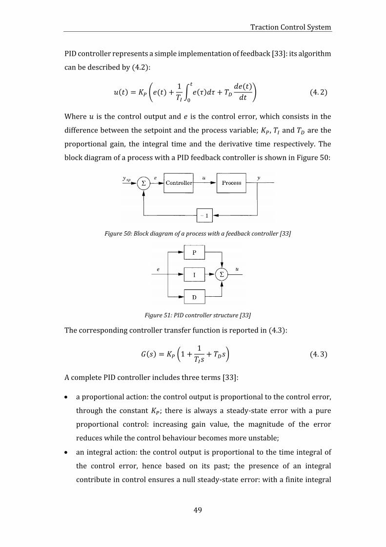
Traction Control System
49
PID controller represents a simple implementation of feedback [33]: its algorithm
can be described by (4.2):
𝑢(𝑡) = 𝐾𝑃 (𝑒(𝑡) +1
𝑇𝐼∫ 𝑒(𝜏)𝑑𝜏𝑡
0
+ 𝑇𝐷𝑑𝑒(𝑡)
𝑑𝑡) (4. 2)
Where 𝑢 is the control output and 𝑒 is the control error, which consists in the
difference between the setpoint and the process variable; 𝐾𝑃, 𝑇𝐼 and 𝑇𝐷 are the
proportional gain, the integral time and the derivative time respectively. The
block diagram of a process with a PID feedback controller is shown in Figure 50:
Figure 50: Block diagram of a process with a feedback controller [33]
Figure 51: PID controller structure [33]
The corresponding controller transfer function is reported in (4.3):
𝐺(𝑠) = 𝐾𝑃 (1 +1
𝑇𝐼𝑠+ 𝑇𝐷𝑠) (4. 3)
A complete PID controller includes three terms [33]:
• a proportional action: the control output is proportional to the control error,
through the constant 𝐾𝑃; there is always a steady-state error with a pure
proportional control: increasing gain value, the magnitude of the error
reduces while the control behaviour becomes more unstable;
• an integral action: the control output is proportional to the time integral of
the control error, hence based on its past; the presence of an integral
contribute in control ensures a null steady-state error: with a finite integral
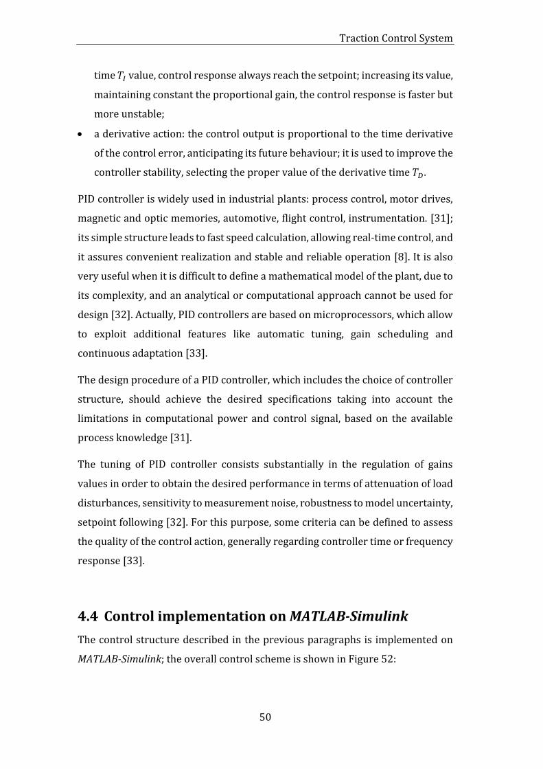
Traction Control System
50
time 𝑇𝐼 value, control response always reach the setpoint; increasing its value,
maintaining constant the proportional gain, the control response is faster but
more unstable;
• a derivative action: the control output is proportional to the time derivative
of the control error, anticipating its future behaviour; it is used to improve the
controller stability, selecting the proper value of the derivative time 𝑇𝐷.
PID controller is widely used in industrial plants: process control, motor drives,
magnetic and optic memories, automotive, flight control, instrumentation. [31];
its simple structure leads to fast speed calculation, allowing real-time control, and
it assures convenient realization and stable and reliable operation [8]. It is also
very useful when it is difficult to define a mathematical model of the plant, due to
its complexity, and an analytical or computational approach cannot be used for
design [32]. Actually, PID controllers are based on microprocessors, which allow
to exploit additional features like automatic tuning, gain scheduling and
continuous adaptation [33].
The design procedure of a PID controller, which includes the choice of controller
structure, should achieve the desired specifications taking into account the
limitations in computational power and control signal, based on the available
process knowledge [31].
The tuning of PID controller consists substantially in the regulation of gains
values in order to obtain the desired performance in terms of attenuation of load
disturbances, sensitivity to measurement noise, robustness to model uncertainty,
setpoint following [32]. For this purpose, some criteria can be defined to assess
the quality of the control action, generally regarding controller time or frequency
response [33].
4.4 Control implementation on MATLAB-Simulink
The control structure described in the previous paragraphs is implemented on
MATLAB-Simulink; the overall control scheme is shown in Figure 52:
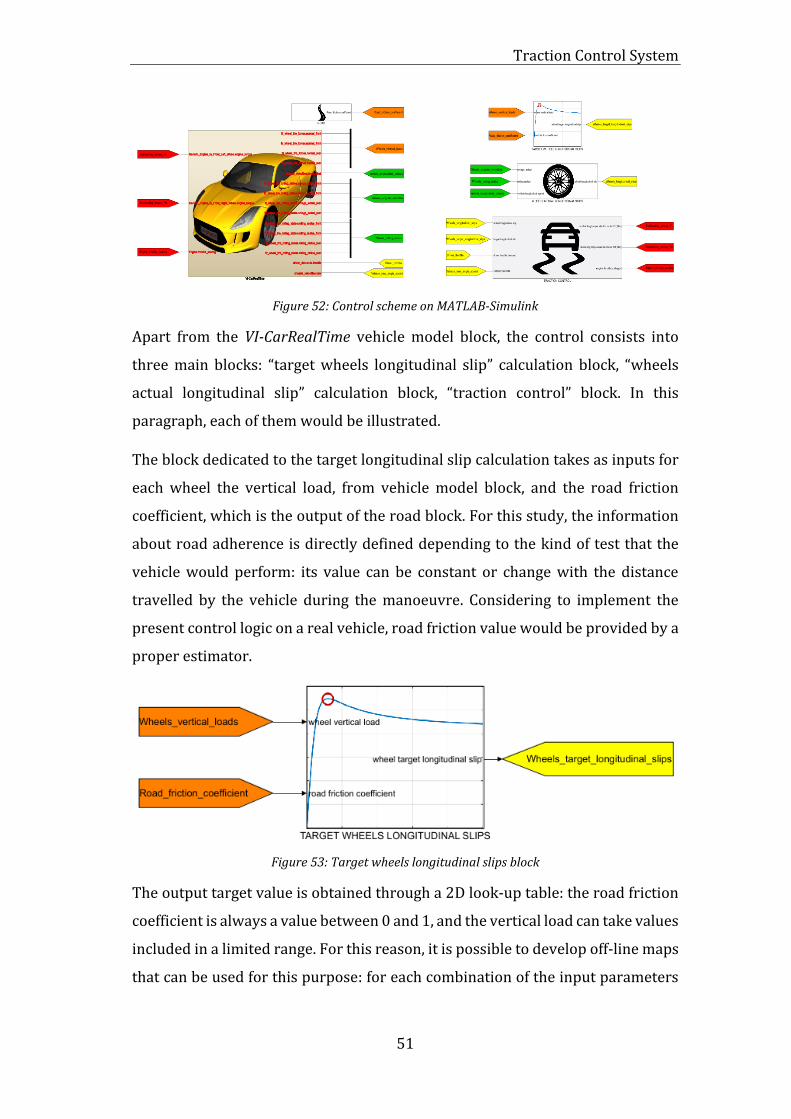
Traction Control System
51
Figure 52: Control scheme on MATLAB-Simulink
Apart from the VI-CarRealTime vehicle model block, the control consists into
three main blocks: “target wheels longitudinal slip” calculation block, “wheels
actual longitudinal slip” calculation block, “traction control” block. In this
paragraph, each of them would be illustrated.
The block dedicated to the target longitudinal slip calculation takes as inputs for
each wheel the vertical load, from vehicle model block, and the road friction
coefficient, which is the output of the road block. For this study, the information
about road adherence is directly defined depending to the kind of test that the
vehicle would perform: its value can be constant or change with the distance
travelled by the vehicle during the manoeuvre. Considering to implement the
present control logic on a real vehicle, road friction value would be provided by a
proper estimator.
Figure 53: Target wheels longitudinal slips block
The output target value is obtained through a 2D look-up table: the road friction
coefficient is always a value between 0 and 1, and the vertical load can take values
included in a limited range. For this reason, it is possible to develop off-line maps
that can be used for this purpose: for each combination of the input parameters
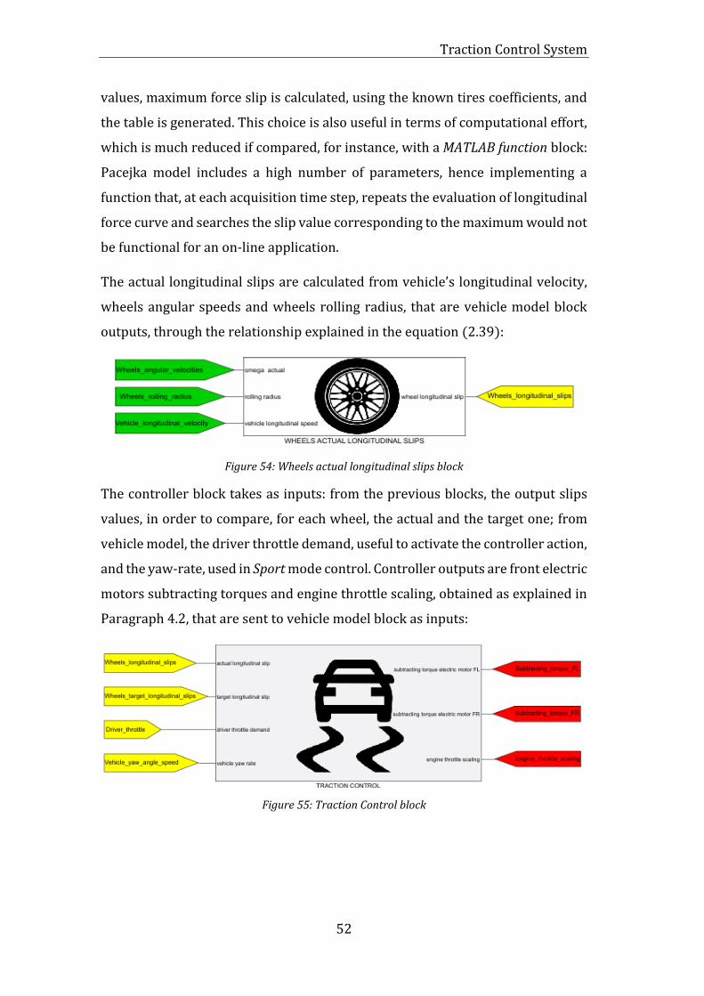
Traction Control System
52
values, maximum force slip is calculated, using the known tires coefficients, and
the table is generated. This choice is also useful in terms of computational effort,
which is much reduced if compared, for instance, with a MATLAB function block:
Pacejka model includes a high number of parameters, hence implementing a
function that, at each acquisition time step, repeats the evaluation of longitudinal
force curve and searches the slip value corresponding to the maximum would not
be functional for an on-line application.
The actual longitudinal slips are calculated from vehicle’s longitudinal velocity,
wheels angular speeds and wheels rolling radius, that are vehicle model block
outputs, through the relationship explained in the equation (2.39):
Figure 54: Wheels actual longitudinal slips block
The controller block takes as inputs: from the previous blocks, the output slips
values, in order to compare, for each wheel, the actual and the target one; from
vehicle model, the driver throttle demand, useful to activate the controller action,
and the yaw-rate, used in Sport mode control. Controller outputs are front electric
motors subtracting torques and engine throttle scaling, obtained as explained in
Paragraph 4.2, that are sent to vehicle model block as inputs:
Figure 55: Traction Control block
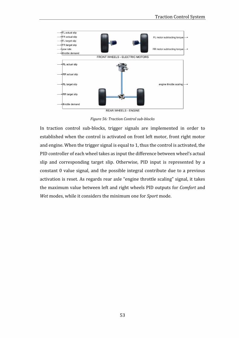
Traction Control System
53
Figure 56: Traction Control sub-blocks
In traction control sub-blocks, trigger signals are implemented in order to
established when the control is activated on front left motor, front right motor
and engine. When the trigger signal is equal to 1, thus the control is activated, the
PID controller of each wheel takes as input the difference between wheel’s actual
slip and corresponding target slip. Otherwise, PID input is represented by a
constant 0 value signal, and the possible integral contribute due to a previous
activation is reset. As regards rear axle “engine throttle scaling” signal, it takes
the maximum value between left and right wheels PID outputs for Comfort and
Wet modes, while it considers the minimum one for Sport mode.
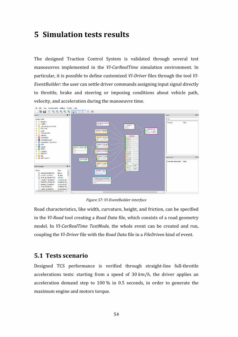
54
5 Simulation tests results
The designed Traction Control System is validated through several test
manoeuvres implemented in the VI-CarRealTime simulation environment. In
particular, it is possible to define customized VI-Driver files through the tool VI-
EventBuilder: the user can settle driver commands assigning input signal directly
to throttle, brake and steering or imposing conditions about vehicle path,
velocity, and acceleration during the manoeuvre time.
Figure 57: VI-EventBuilder interface
Road characteristics, like width, curvature, height, and friction, can be specified
in the VI-Road tool creating a Road Data file, which consists of a road geometry
model. In VI-CarRealTime TestMode, the whole event can be created and run,
coupling the VI-Driver file with the Road Data file in a FileDriven kind of event.
5.1 Tests scenario
Designed TCS performance is verified through straight-line full-throttle
accelerations tests: starting from a speed of 30 𝑘𝑚/ℎ, the driver applies an
acceleration demand step to 100 % in 0.5 seconds, in order to generate the
maximum engine and motors torque.

Simulation tests results
55
Figure 58: Driver throttle demand during acceleration manoeuvre
The manoeuvre is carried out on three different road conditions:
• Mu-split: a mu-split road surface is characterized by different adhesion
coefficient on the right and left side. On this kind of road, a vehicle without
TCS would lose its stability during acceleration because of the different
traction of wheels on the two vehicle’s sides. If TCS is active on the vehicle, it
should help to maintain the straight-line path without requiring a significant
driver effort.
Figure 59: Road friction coefficients during mu-split manoeuvre
• Variable Mu-split: the road shows different friction coefficients on its two
sides, with a variable value during the acceleration: from 1 to 0.5 and then 0.7
for the right side, from 0.4 to 0.8 and then 0.5 for the left one. For this test, a

Simulation tests results
56
vehicle behaviour similar to the constant Mu-split case is expected, and, in
addition, the robustness of control against fast-changing road conditions can
be analysed.
Figure 60: Road friction coefficients on variable mu-split manoeuvre
• Low friction: the road surface has a uniform low friction coefficient, which
reproduces wet conditions. In this case, all the wheels of the passive vehicle
lose their adhesion with the road because of their excessive slips; as explained
in Paragraph 4.1, this situation represents a dangerous condition because
none of the vehicle wheels would be able to generate force the in lateral
direction, hence in presence of a steering driver demand the vehicle would
react with an unstable behaviour. The TC system attempts to limit each wheel
slip, making the most of surface friction and enhancing vehicle traction.
Figure 61: Road friction coefficients during low friction manoeuvre

Simulation tests results
57
5.2 Comparison with passive vehicle
The developed algorithm’s effectiveness is demonstrated through a comparison
between the vehicle equipped with TC and the passive vehicle, performing the
simulations of the three described scenarios.
5.2.1 Mu-split road
The simulation outputs included in the time range between 7 and 13 seconds,
which is involved by the control activation, are reported.
Figure 62: Wheels longitudinal slips during mu-split test
Considering the results shown in Figure 62 after the acceleration command, the
rotational speed of passive vehicle right wheels, which are in contact with lower
adhesion coefficient, diverges rapidly, as expected. On the rear axle, owing to the
LSD differential action, also the left wheel starts to spin: the differential transfers
a higher torque to the traction wheel in order to accelerate it, until it reaches the
same longitudinal slip value of the right wheel, which receives a lower torque.
This condition leads the vehicle to the instability, confirmed by the steering wheel
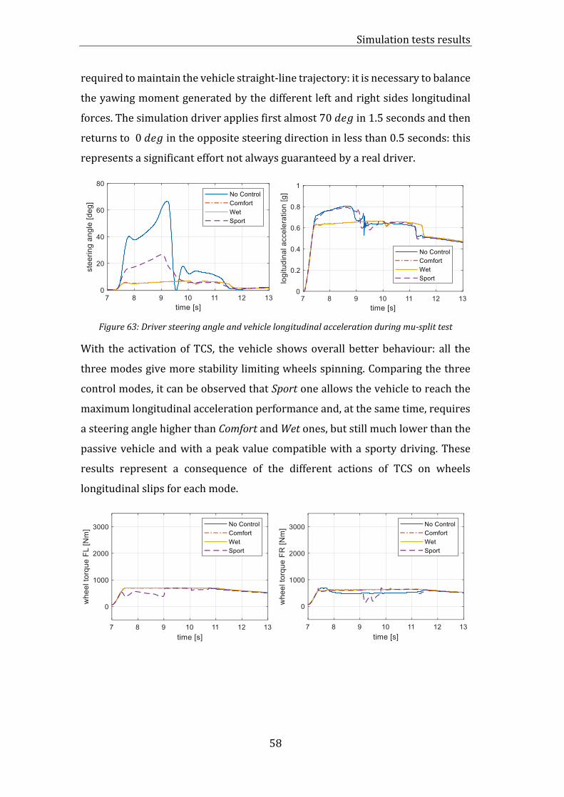
Simulation tests results
58
required to maintain the vehicle straight-line trajectory: it is necessary to balance
the yawing moment generated by the different left and right sides longitudinal
forces. The simulation driver applies first almost 70 𝑑𝑒𝑔 in 1.5 seconds and then
returns to 0 𝑑𝑒𝑔 in the opposite steering direction in less than 0.5 seconds: this
represents a significant effort not always guaranteed by a real driver.
Figure 63: Driver steering angle and vehicle longitudinal acceleration during mu-split test
With the activation of TCS, the vehicle shows overall better behaviour: all the
three modes give more stability limiting wheels spinning. Comparing the three
control modes, it can be observed that Sport one allows the vehicle to reach the
maximum longitudinal acceleration performance and, at the same time, requires
a steering angle higher than Comfort and Wet ones, but still much lower than the
passive vehicle and with a peak value compatible with a sporty driving. These
results represent a consequence of the different actions of TCS on wheels
longitudinal slips for each mode.
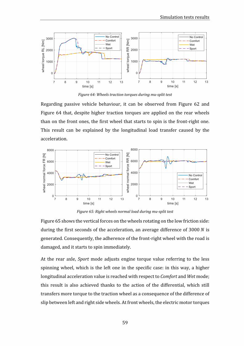
Simulation tests results
59
Figure 64: Wheels traction torques during mu-split test
Regarding passive vehicle behaviour, it can be observed from Figure 62 and
Figure 64 that, despite higher traction torques are applied on the rear wheels
than on the front ones, the first wheel that starts to spin is the front-right one.
This result can be explained by the longitudinal load transfer caused by the
acceleration.
Figure 65: Right wheels normal load during mu-split test
Figure 65 shows the vertical forces on the wheels rotating on the low friction side:
during the first seconds of the acceleration, an average difference of 3000 𝑁 is
generated. Consequently, the adherence of the front-right wheel with the road is
damaged, and it starts to spin immediately.
At the rear axle, Sport mode adjusts engine torque value referring to the less
spinning wheel, which is the left one in the specific case: in this way, a higher
longitudinal acceleration value is reached with respect to Comfort and Wet mode;
this result is also achieved thanks to the action of the differential, which still
transfers more torque to the traction wheel as a consequence of the difference of
slip between left and right side wheels. At front wheels, the electric motor torques

Simulation tests results
60
exhibited in Figure 64 result from both longitudinal slips and yaw-rate controls:
without the last of them, only the right motor torque would be reduced to
regulate the wheel spinning, while, in this case, further subtracting torque
contributes can be observed. It is possible to compare driver steering and driver
steering speed of Sport mode considering the cases of yaw-rate control and no
yaw-rate control to verify its performance, as shown in Figure 66:
Figure 66: Driver steering angle and driver steering angle speed during mu-split test (Sport mode)
The yaw-rate control presence permits a reduction of the maximum steering
angle required to the driver, from 30 𝑑𝑒𝑔 to 26 𝑑𝑒𝑔, and of steering oscillations
in general, confirmed by lower peak values of steering velocity.
Figure 67: Vehicle yaw-rate and longitudinal acceleration during mu-split test (Sport mode)
Since for this manoeuvre the yaw-rate control activation causes only a reduction
of front motors traction torque, it follows that also the overall vehicle longitudinal
acceleration is reduced. However, this effect is considered acceptable if compared
with the advantages in terms of vehicle stability. Furthermore, it has to be noticed
that, during acceleration, the longitudinal load transfer increases the rear axle
wheels vertical load; as a result, most of vehicle longitudinal acceleration is due
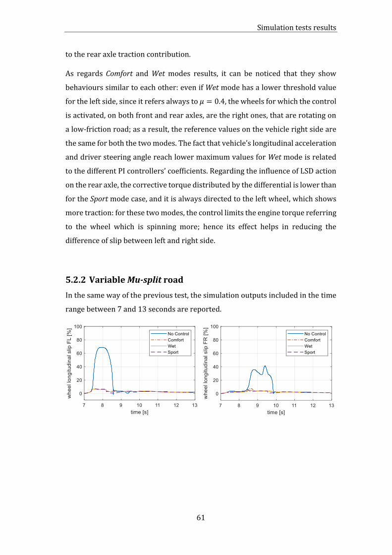
Simulation tests results
61
to the rear axle traction contribution.
As regards Comfort and Wet modes results, it can be noticed that they show
behaviours similar to each other: even if Wet mode has a lower threshold value
for the left side, since it refers always to 𝜇 = 0.4, the wheels for which the control
is activated, on both front and rear axles, are the right ones, that are rotating on
a low-friction road; as a result, the reference values on the vehicle right side are
the same for both the two modes. The fact that vehicle’s longitudinal acceleration
and driver steering angle reach lower maximum values for Wet mode is related
to the different PI controllers’ coefficients. Regarding the influence of LSD action
on the rear axle, the corrective torque distributed by the differential is lower than
for the Sport mode case, and it is always directed to the left wheel, which shows
more traction: for these two modes, the control limits the engine torque referring
to the wheel which is spinning more; hence its effect helps in reducing the
difference of slip between left and right side.
5.2.2 Variable Mu-split road
In the same way of the previous test, the simulation outputs included in the time
range between 7 and 13 seconds are reported.
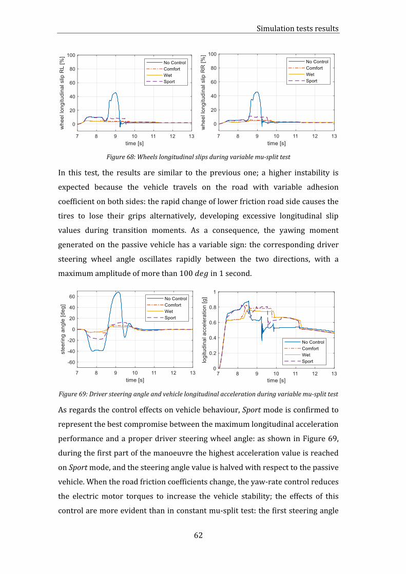
Simulation tests results
62
Figure 68: Wheels longitudinal slips during variable mu-split test
In this test, the results are similar to the previous one; a higher instability is
expected because the vehicle travels on the road with variable adhesion
coefficient on both sides: the rapid change of lower friction road side causes the
tires to lose their grips alternatively, developing excessive longitudinal slip
values during transition moments. As a consequence, the yawing moment
generated on the passive vehicle has a variable sign: the corresponding driver
steering wheel angle oscillates rapidly between the two directions, with a
maximum amplitude of more than 100 𝑑𝑒𝑔 in 1 second.
Figure 69: Driver steering angle and vehicle longitudinal acceleration during variable mu-split test
As regards the control effects on vehicle behaviour, Sport mode is confirmed to
represent the best compromise between the maximum longitudinal acceleration
performance and a proper driver steering wheel angle: as shown in Figure 69,
during the first part of the manoeuvre the highest acceleration value is reached
on Sport mode, and the steering angle value is halved with respect to the passive
vehicle. When the road friction coefficients change, the yaw-rate control reduces
the electric motor torques to increase the vehicle stability; the effects of this
control are more evident than in constant mu-split test: the first steering angle
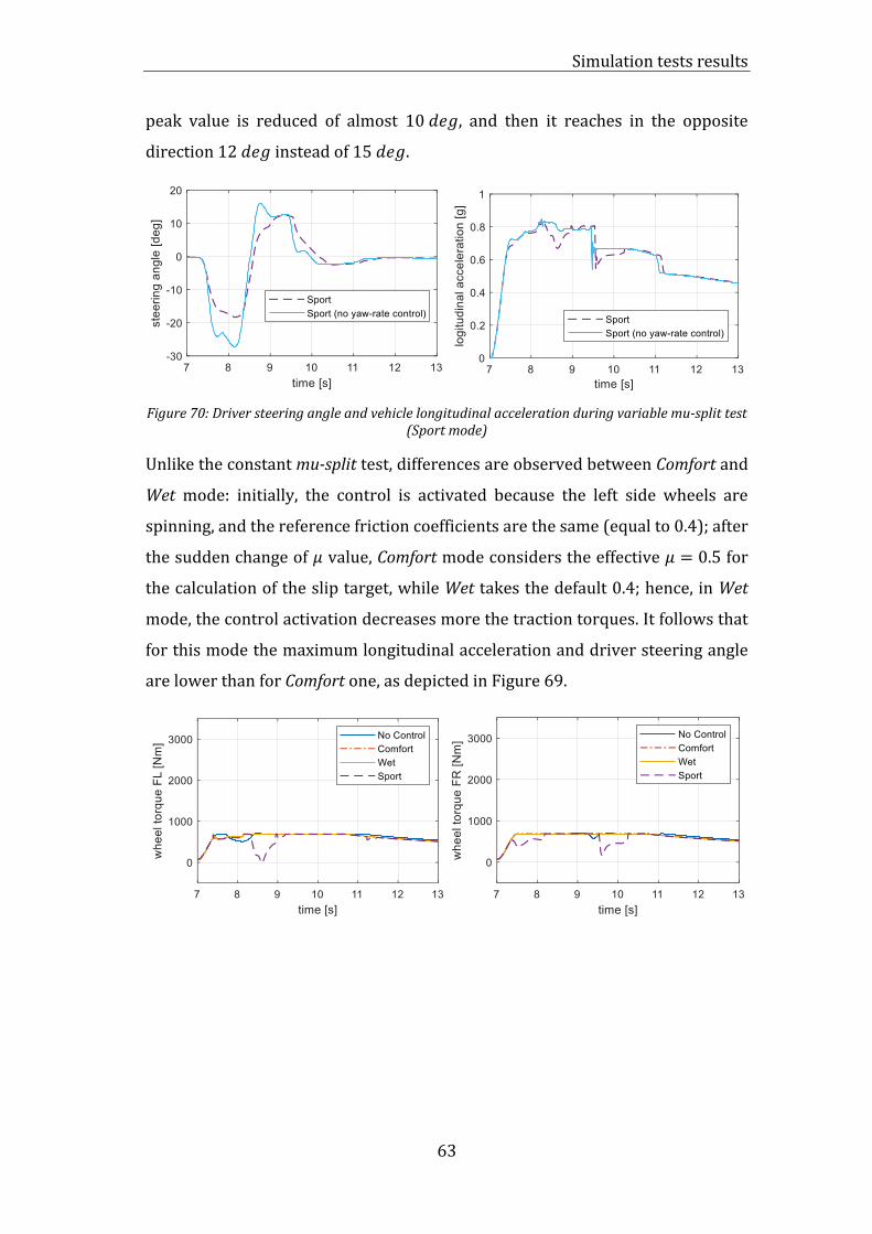
Simulation tests results
63
peak value is reduced of almost 10 𝑑𝑒𝑔, and then it reaches in the opposite
direction 12 𝑑𝑒𝑔 instead of 15 𝑑𝑒𝑔.
Figure 70: Driver steering angle and vehicle longitudinal acceleration during variable mu-split test (Sport mode)
Unlike the constant mu-split test, differences are observed between Comfort and
Wet mode: initially, the control is activated because the left side wheels are
spinning, and the reference friction coefficients are the same (equal to 0.4); after
the sudden change of 𝜇 value, Comfort mode considers the effective 𝜇 = 0.5 for
the calculation of the slip target, while Wet takes the default 0.4; hence, in Wet
mode, the control activation decreases more the traction torques. It follows that
for this mode the maximum longitudinal acceleration and driver steering angle
are lower than for Comfort one, as depicted in Figure 69.

Simulation tests results
64
Figure 71: Wheels traction torque during variable mu-split test
5.2.3 Low friction road
During this test, the target road friction value is 0.4 for all the control modes, as a
consequence, the results on vehicle behaviour are expected to be differentiated
only for the contribute of PI coefficients value. The simulation outputs included
in the time range between 7 and 17 seconds are reported.
Figure 72: Wheels longitudinal slips during low friction test
As regards the passive vehicle, it can be observed from Figure 72 that all the
wheels exceed the limit: the instability due to the loss of adherence requires a

Simulation tests results
65
reaction of the driver with a steering command to maintain the trajectory, after a
few seconds from the initial acceleration command. With the TC intervention, the
driver steering effort is nulled: for each axle, left and right wheels are rotating
with the same speed, with small slip values, and are subjected to the same
working conditions. On the rear axle, the engine torque reduced by the control is
distributed equally by the differential, and the same longitudinal forces are
developed on both axle sides; as a result, no yawing moment is generated, and
the vehicle maintains the straight-line trajectory.
Figure 73: Driver steering angle and vehicle longitudinal acceleration during low friction test
Unlike the mu-split tests, it can be observed from Figure 72 that on the passive
vehicle all the wheels on the low surface start to spin immediately: during this
manoeuvre smaller longitudinal acceleration is reached and the longitudinal load
transfer is lower, consequently all the wheels lose quickly the adherence with the
road.
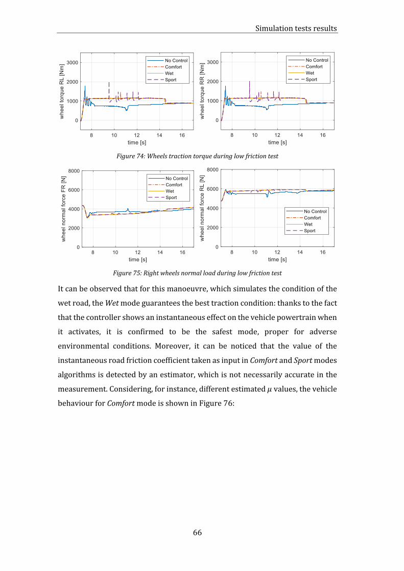
Simulation tests results
66
Figure 74: Wheels traction torque during low friction test
Figure 75: Right wheels normal load during low friction test
It can be observed that for this manoeuvre, which simulates the condition of the
wet road, the Wet mode guarantees the best traction condition: thanks to the fact
that the controller shows an instantaneous effect on the vehicle powertrain when
it activates, it is confirmed to be the safest mode, proper for adverse
environmental conditions. Moreover, it can be noticed that the value of the
instantaneous road friction coefficient taken as input in Comfort and Sport modes
algorithms is detected by an estimator, which is not necessarily accurate in the
measurement. Considering, for instance, different estimated 𝜇 values, the vehicle
behaviour for Comfort mode is shown in Figure 76:
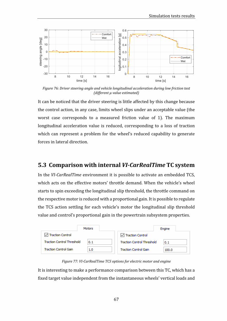
Simulation tests results
67
Figure 76: Driver steering angle and vehicle longitudinal acceleration during low friction test (different 𝜇 value estimated)
It can be noticed that the driver steering is little affected by this change because
the control action, in any case, limits wheel slips under an acceptable value (the
worst case corresponds to a measured friction value of 1). The maximum
longitudinal acceleration value is reduced, corresponding to a loss of traction
which can represent a problem for the wheel’s reduced capability to generate
forces in lateral direction.
5.3 Comparison with internal VI-CarRealTime TC system
In the VI-CarRealTime environment it is possible to activate an embedded TCS,
which acts on the effective motors’ throttle demand. When the vehicle’s wheel
starts to spin exceeding the longitudinal slip threshold, the throttle command on
the respective motor is reduced with a proportional gain. It is possible to regulate
the TCS action settling for each vehicle’s motor the longitudinal slip threshold
value and control’s proportional gain in the powertrain subsystem properties.
Figure 77: VI-CarRealTime TCS options for electric motor and engine
It is interesting to make a performance comparison between this TC, which has a
fixed target value independent from the instantaneous wheels’ vertical loads and

Simulation tests results
68
friction coefficients, and the Comfort and Sport modes of the proposed control
method.
The first test considered is the acceleration on constant mu-split road described
in Paragraph 5.2.1: the simulation outputs are reported in Figure 78.
Figure 78: Comparison of designed TC (Comfort and Sport modes) and VI-CRT TC on mu-split test: driver steering angle, longitudinal acceleration, wheels longitudinal slips
It can be observed that the results of VI-CRT control are a middle ground between
the Comfort mode vehicle behaviour and the Sport mode one. The vehicle reaches
higher longitudinal acceleration than Comfort mode, but not the maximum
possible value. On FR wheel, the VI-CRT target is higher than the value at which
the tire generates the maximum longitudinal ground force because the control is
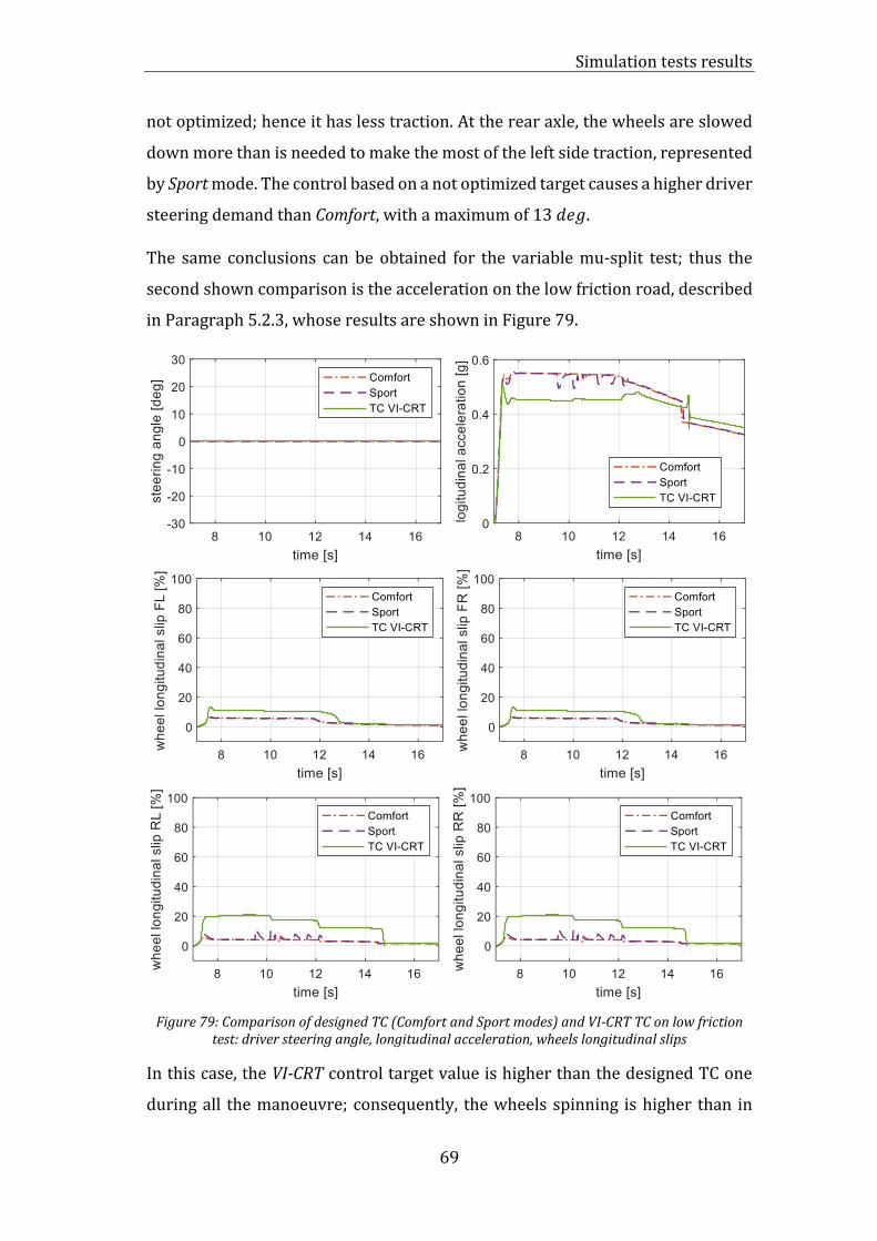
Simulation tests results
69
not optimized; hence it has less traction. At the rear axle, the wheels are slowed
down more than is needed to make the most of the left side traction, represented
by Sport mode. The control based on a not optimized target causes a higher driver
steering demand than Comfort, with a maximum of 13 𝑑𝑒𝑔.
The same conclusions can be obtained for the variable mu-split test; thus the
second shown comparison is the acceleration on the low friction road, described
in Paragraph 5.2.3, whose results are shown in Figure 79.
Figure 79: Comparison of designed TC (Comfort and Sport modes) and VI-CRT TC on low friction test: driver steering angle, longitudinal acceleration, wheels longitudinal slips
In this case, the VI-CRT control target value is higher than the designed TC one
during all the manoeuvre; consequently, the wheels spinning is higher than in
Simulation tests results
70
Comfort and Sport modes both, and the vehicle loses traction. On the straight-line
manoeuvre, there is no evidence of vehicle instability because the VI-CRT control
still limits wheels slips, and the wheels of the same axle rotate at the same speed
hence no yawing moment is generated; however, this condition can represent a
problem in case of request of wheel lateral ground forces.

71
6 Driving Simulator results
The three control modes are tested on a dynamic driving simulator: the same
vehicle model used for VI-CarRealTime off-line simulations is implemented on the
simulator system, and comparisons between passive and active vehicles can be
made in terms of driver feeling.
The simulator is called dynamic since it is characterized by a motion system that
provides accurate feedback to the driver about vehicle handling and ride
behaviour. For this work, in particular, the tests are carried on the Danisi
Engineering dynamic simulator, provided by VI-Grade, which is equipped with a
nine-degrees-of-freedom moving platform, called Driver in Motion (DiM) [34].
Figure 80: Danisi Engineering dynamic driving simulator [35]
In addition to precise motion perception, the real driving situation feeling is also
given by the virtual environment surrounding the simulator. First of all, the
driver sits in a real cabin taken from a vehicle, and a virtual road scene is
projected on a screen all around him: the visual system is necessary to give the
driver the correct impression about vehicle speed and movement. To obtain a
realistic driver interaction with commands, the simulator cockpit is equipped
with additional actuators that imitate faithfully the feel of pedal and steering
wheel. Engine and driving noises are also reproduced, depending on engine
Driving Simulator results
72
power, engine speed, and driving speed, to let the driver perceive the external
environment as realistically as possible [36].
Using driving simulator tests leads to many advantages: it permits to identify
problems earlier in the design process [34], and to correct them reducing
systems’ development times and costs. With respect to road tests, driving
simulator ones guarantee: no risks for the driver and the environment, allowing
a safe representation of critical driving situations; the possibility to repeat the
same test with identical conditions many times, showing high reproducibility;
quick and simple changes of vehicle and environment (tracks, weather
conditions) parameters [36]. For this study, the dynamic driving simulator is
exploited to assess the designed TC system’s effectiveness reproducing the same
road scenarios analysed in Paragraph 5.1.
6.1 Tests executions
Before starting tests executions, it is necessary to let the driving simulator system
communicate with the control logic designed on Simulink. First of all, the VI-
CarRealTime vehicle model is implemented on the simulator to obtain the same
handling and ride dynamic responses of off-line tests. Then, road scenarios are
created: infinite straight-line roads with high friction (𝜇 = 1), low friction (𝜇 =
0.4) and mu-split (𝜇𝑙𝑒𝑓𝑡 = 1, 𝜇𝑟𝑖𝑔ℎ𝑡 = 0.4) surface respectively.
The Simulink scheme is rearranged to be compatible with the simulator: the
vehicle model block is substituted by more blocks, each of them representing the
corresponding input or output simulator channel. The new scheme is then
compiled and then uploaded on the system. Regarding the electric motors, the
acquisition of the subtractive torques, generated by the control in case of
activation, have to be specified to the system before starting the tests.
After setting all these initial aspects, the maximum acceleration performances are
executed. The first test is made on a mu-split surface: starting from 30 𝑘𝑚/ℎ, the
driver imposes a 100 % throttle step demand and tries to maintain the straight-
line trajectory. The same manoeuvre is repeated with the passive vehicle and the
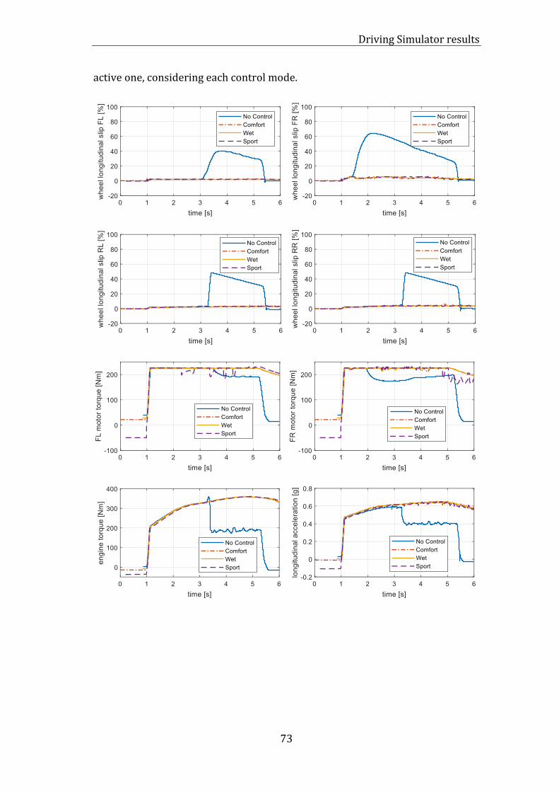
Driving Simulator results
73
active one, considering each control mode.

Driving Simulator results
74
Figure 81: Results of mu-split manoeuvre: wheel longitudinal slips, motors and engine torque, vehicle longitudinal acceleration, driver steering angle, vehicle trajectory
As shown in Figure 81, the driver steering reaction is not sufficient to maintain
vehicle control and guarantee the straight-line trajectory on the passive vehicle.
Initially, only the front-right wheel starts to rotate excessively, due to the
significant longitudinal load transfer during the acceleration, as explained for off-
line performance. The driver does not immediately perceive the loss of adherence
on the right side of the vehicle, but after a few moments, when the vehicle has
already lost its stability. This unstable condition does not permit to reach good
acceleration performance. Instead, as can be seen by the trajectory plot, the
vehicle goes on the right side of the road: this also causes the front-left wheel’s
spinning, changing from high to low friction surface.
With the control activation, the vehicle shows higher stability. It reaches higher
longitudinal values and maintains the straight-line trajectory with a small driver
steering effort: the required steering angle maximum value is lower than 10 𝑑𝑒𝑔
for all the three modes.
Unlike the corresponding off-line test, there are no significant differences
between Sport mode and the other two ones. In the first part of the acceleration,
only the front-right wheel causes the control activation; hence the vehicle
response is similar for each control mode. When also the rear axle wheels spin,
the Sport modes provide a slightly higher engine torque. During all the duration
of the manoeuvre, Sport mode acceleration performance is penalized by the yaw-
rate control, which reduces the torque of front-left and front-right motor
alternatively. Consequently, it can be affirmed that the vehicle behaviour seems
to be substantially the same for all the three control modes in a simulation of the
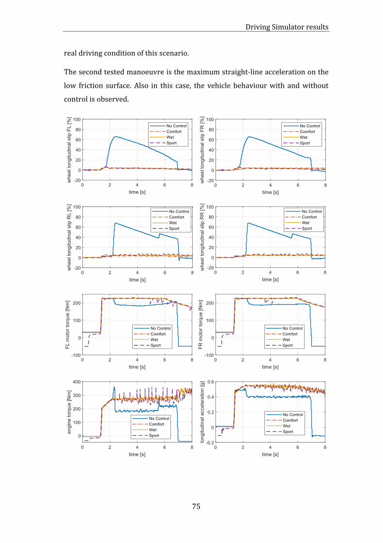
Driving Simulator results
75
real driving condition of this scenario.
The second tested manoeuvre is the maximum straight-line acceleration on the
low friction surface. Also in this case, the vehicle behaviour with and without
control is observed.

Driving Simulator results
76
Figure 82: Results of low friction manoeuvre: wheel longitudinal slips, motors and engine torque, vehicle longitudinal acceleration, driver steering angle, vehicle trajectory
On the passive vehicle, all the four wheels lose adherence with the road, and, as a
consequence, the vehicle becomes unstable. Even if the driver reacts with a
steering angle demand that reaches a maximum value of 60 𝑑𝑒𝑔, it is not
sufficient to maintain the trajectory: he loses the vehicle control.
With the control activation, the wheels’ rotation is maintained under a threshold.
In the same way of the relative off-line test, for each control modes the limit slip
value of all the wheels is calculated referring to a road friction coefficient of 0.4,
thus the differences among them are due to PI controllers’ coefficients.
All the three modes allow the vehicle to achieve a satisfactory longitudinal
acceleration during all the manoeuvre, while maintaining its directional stability
without driver steering effort: the maximum steering value is 1 𝑑𝑒𝑔, while the
maximum lateral displacement with respect to the straight-line trajectory is less
than 1 𝑚. This behaviour is the result of the good functioning of all three control
modes in general. Considering the wheels slips value, it can be noticed that on
front wheels there are no differences between Sport, Comfort, and Wet: for Sport
mode, the slips values are slightly decreased when the yaw-rate control activates,
but the reductions are not significant. The different controllers tuning is evident
on the rear axle: Sport throttle scaling command on engine torque is more
fluctuating than Comfort and Wet ones. As a result, it can be observed that, during
the acceleration, rear wheels slips have higher peak values for Sport mode than
for Comfort and Wet ones. This aspect influences vehicle acceleration
performance: in Comfort and Wet modes, the rear wheels instantaneously acquire
grip with the road, and the vehicle shows overall better traction than in Sport
Driving Simulator results
77
mode.
For this manoeuvre scenario, it can be affirmed that the on-line test confirms the
result of the off-line simulation.
6.2 Driver feedback
One of the advantages of the driving simulator tests is collecting the professional
driver feedback about the vehicle’s dynamic behaviour during the manoeuvres’
performance. In this way, it is possible to change rapidly vehicle model
parameters and/or, for this specific case, PI controllers’ coefficients in order to
reach the desired target. This process would not be easy and fast with road
testing, because it involves physical components’ changes and software’s
updates. Different configurations can be tested with a driving simulator, and the
driver’s feelings can be taken into account while evaluating the best solution.
For this study, it is important to know driver’s feedback about how the control
activation changes the vehicle response to his acceleration command. For both
the test manoeuvres, in general the presence of the traction control helped the
driver maintain the trajectory without a great steering effort. While repeating the
acceleration on mu-split or low friction surface, in some cases it was necessary to
apply a high steering angle value to complete the manoeuvre. However, the
lateral displacement of the vehicle was not negligible: in a real driving situation,
it would correspond to a change of roadway, which can be dangerous if
considering a normal traffic condition. In the other cases, the driver lost the
vehicle control because his reaction wasn’t quick enough. As a consequence, the
active vehicle makes him feel more comfortable and safer while performing the
manoeuvre.
On the other hand, the three modes’ differences are not so evident from the
driver’s point of view. In particular, the driver perception is that Comfort and Wet
modes decrease the powertrain torques in a stabler way than Sport mode:
especially on the rear axle, the torque is reduced instantaneously and without
fluctuation, which gives the impression of a more “linear” recovery of vehicle
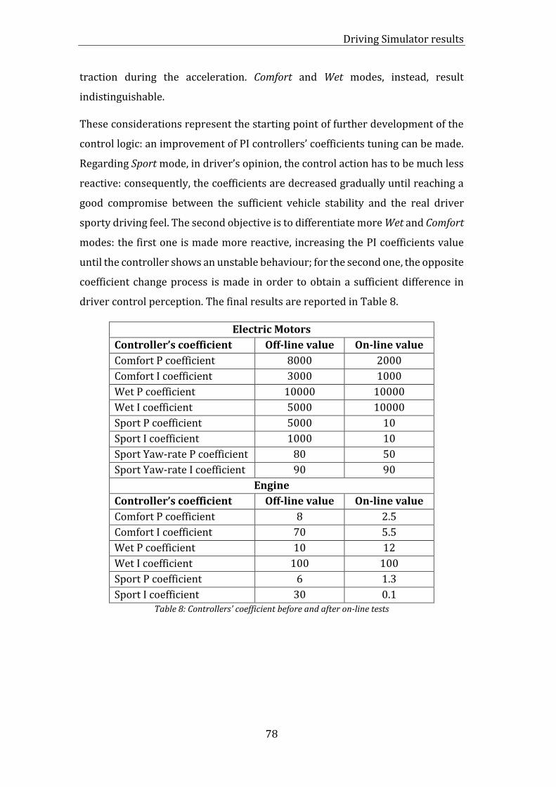
Driving Simulator results
78
traction during the acceleration. Comfort and Wet modes, instead, result
indistinguishable.
These considerations represent the starting point of further development of the
control logic: an improvement of PI controllers’ coefficients tuning can be made.
Regarding Sport mode, in driver’s opinion, the control action has to be much less
reactive: consequently, the coefficients are decreased gradually until reaching a
good compromise between the sufficient vehicle stability and the real driver
sporty driving feel. The second objective is to differentiate more Wet and Comfort
modes: the first one is made more reactive, increasing the PI coefficients value
until the controller shows an unstable behaviour; for the second one, the opposite
coefficient change process is made in order to obtain a sufficient difference in
driver control perception. The final results are reported in Table 8.
Electric Motors
Controller’s coefficient Off-line value On-line value
Comfort P coefficient 8000 2000
Comfort I coefficient 3000 1000
Wet P coefficient 10000 10000
Wet I coefficient 5000 10000
Sport P coefficient 5000 10
Sport I coefficient 1000 10
Sport Yaw-rate P coefficient 80 50
Sport Yaw-rate I coefficient 90 90
Engine
Controller’s coefficient Off-line value On-line value
Comfort P coefficient 8 2.5
Comfort I coefficient 70 5.5
Wet P coefficient 10 12
Wet I coefficient 100 100
Sport P coefficient 6 1.3
Sport I coefficient 30 0.1 Table 8: Controllers' coefficient before and after on-line tests

79
7 Conclusions
In this thesis, a Traction Control System algorithm for an All-Wheel-Drive hybrid
vehicle is developed. In particular, the control is applied to a high-performance
vehicle whose dynamic behaviour can be adapted setting three different driving
modes: Comfort, Wet, and Sport. The control acts on the vehicle powertrain,
reducing the tractive torque when the driving wheels rotate excessively. Each of
the two front wheels is connected to the corresponding onboard electric motor;
hence the torque control is activated independently on the single spinning wheel.
On the rear axle, both of the wheels are moved by a thermal engine whose torque
is distributed by an LSD differential: depending on the control mode, when one
or both the wheels exceed the slip limit value, the engine output torque is reduced
closing the throttle valve. The effectiveness of the control activation is assessed
through full-throttle straight-line acceleration manoeuvres, performed with off-
line tests, on VI-CarRealTime and MATLAB-Simulink software, and on-line ones,
on a dynamic driving simulator.
Analysing test results, it can be observed that the control improves the vehicle
stability: as regards off-line tests, the driving torque reduction prevents the
wheels from spinning and allows the driver to reduce the steering effort
necessary to maintain the straight-line trajectory. The maximum steering angle
value decreases from Sport to Comfort and Wet modes: this result confirms that
the last two ones are more focused on vehicle safety. In general, on the active
vehicle the wheels’ longitudinal slips show low values; hence the vehicle itself
always maintains the grip with the road and achieves a higher maximum
longitudinal acceleration. The acceleration performance is enhanced in Sport
mode, especially when some of the vehicle wheels are on a dry surface: it can be
noticed for the mu-split test that the overall 𝑎𝑥value is higher for this mode; on
the contrary, for a low-friction surface (wet road) the most indicated mode is the
Wet one, because of its fastest controllers’ response.
Similar conclusions can be made considering the driving simulator tests: when

Conclusions
80
the driver accelerates with the passive vehicle, it is difficult for him to maintain
the vehicle control on a low-friction or a mu-split road; with the presence of the
control, he feels more comfortable while performing the manoeuvre, verifying
off-line simulations results. During the on-line tests, the differences among the
three modes result not as evident as for the off-line simulations: the vehicle
dynamic behaviour’s perception is substantially the same when changing from
Sport to Comfort or Wet mode. Starting from this feedback, a further PI
controllers’ tuning process is made: the tests manoeuvres are repeated several
times and the controllers’ coefficients are gradually modified in order to
differentiate more the three modes from the driver point of view, always taking
into account the target of each of them described in Paragraph 4.2.
As a conclusion, thanks to DiM tests and the opportunity to know the professional
driver’s feedback, the final tuning results in a robust, stable and effective Traction
Control System logic.
7.1 Future developments
For this study, the control logic is designed considering that all the inputs
parameters are known: during off-line tests, all the variables values are provided
by the VI-CarRealTime vehicle model; during the on-line ones, the same model is
installed on the driving simulator, which represents a full-sensorized vehicle;
hence all the necessary control input channels are available. This condition is not
satisfied when the control is implemented on a real vehicle; thus, the next steps
for the development of the proposed control regard the deepening of this aspect.
Examples of possible future studies are reported as follows:
1. The two most important control inputs from the vehicle model are the wheels’
vertical loads and the tire/road friction coefficient; both generally cannot be
directly measured but estimated.
As regards the wheels’ normal loads, normally the vehicles are not equipped
with force transducers; hence they have to be evaluated. This is not an easy
task because many factors, such as the change of vehicle mass, the load

Conclusions
81
transfers and the road conditions, affect their value. In [37] an algorithm for
the wheel vertical forces estimation is proposed, which can be applied on
vehicles instrumented with standard sensors.
Different methods and algorithms have been studied to estimate the road
friction coefficient. In [38] the most used approaches are described: they are
substantially divided into model-based and experiment-based methods. The
first ones evaluate the road friction through mathematical models related to
vehicle and wheel dynamics; the second ones correlate the road friction value
to a variable that can be measured with sensors (acoustic, optical,
temperature sensors).
2. The Pacejka maps used to evaluate the target longitudinal slips are based on
known tire coefficients, which correspond to a defined kind of tire. As a
consequence, the algorithm considers the tire to be always the same, while
they change their characteristics during the time and can be substituted. It
would be useful to evaluate, in the range of tires suitable for this kind of
vehicle, how the target longitudinal slip changes, considering all the other
inputs constant. Finally, a set of Pacejka coefficient proper for all the possible
kinds of tires can be defined.

82
Bibliography
[1] K. Reif, Brakes, Brake Control and Driver Assistance Systems: Function,
Regulation and Components, ed. Springer, 2014
[2] L. Shoubo, L. Chenglin, C. Shanglou, W. Lifang, Traction control of Hybrid
Electric Vehicle, 2009 IEEE Vehicle Power and Propulsion Conference,
September 2009, pp. 1535-1540
[3] R. Rajamani, Vehicle dynamics and control, ed. Springer, 2006
[4] D. Song, L. Li, X. Zeng, Y. Jiang, G. Bai, N. Yang, Y. Lei, Traction control-
integrated energy management strategy for all-wheel-drive plug-in hybrid
electric vehicle, Advances in mechanical engineering, December 2017,
Vol.9
[5] W. Chen, Q. Wang, H. Xiao, L. Zhao, M. Zhu, Integrated Vehicle Dynamics and
Control, ed. John Wiley & Sons, 2016
[6] M. M. Abdelhameed, M. Abdelaziz, N. E. Elhady, A. M. Hussein, Development
of integrated brakes and engine traction control system, 15th International
Workshop on Research and Education in Mechatronics (REM), September
2014, pp. 1-5
[7] H.-Z. Li, L. Li, L. He, M.-X. Kang, J. Song, L.-Y. Yu, C. Wu, PID plus fuzzy logic
method for torque control in Traction Control System, International journal
of automotive technology, April 2012, Vol.13 (3), pp. 441-450
[8] L. Jin, M. Ling, J. Li, Development of a new traction control system using ant
colony optimization, Advances in mechanical engineering, August 2018,
Vol.10 (8), pp. 1-12
[9] T. Akiba, R. Shirato, T. Fujita, J. Tamura, A study of Novel Traction Control
Method for Electric Motor Driven Vehicle, 2007 Power Conversion
Conference - Nagoya, April 2007, pp. 699-704
[10] H. Fujimoto, J. Amada, K. Maeda, Review of traction and braking control for
electric vehicle, 2012 IEEE Vehicle Power and Propulsion Conference,
October 2012, pp. 1292-1299
[11] V. Ivanov, D. Savitski, B. Shyrokau, A Survey of Traction Control and
Antilock Braking Systems of Full Electric Vehicles with Individually
Bibliography
83
Controlled Electric Motors, IEEE Transactions on Vehicular Technology,
September 2015, Vol.64(9), pp.3878-3896
[12] S. De Pinto, C. Chatzikomis, A. Sorniotti, G. Mantriota, Comparison of
Traction Controllers for electric Vehicles with On-Board Drivetrains, IEEE
transactions on vehicular technology, August 2017, Vol.66 (8), pp. 6715-
6727
[13] D. Tavernini, M. Metzler, P. Gruber, A. Sorniotti, Explicit Nonlinear Model
Predictive Control for Electric Vehicle Traction Control, IEEE transactions
on control systems technology, July 2019, Vol.27 (4), pp. 1438-1451
[14] S. Li, C. Liao, S. Chen, L. Wang, Traction control of Hybrid electric Vehicle,
2009 IEEE Vehicle Power and Propulsion Conference, September 2009,
pp. 1535-1540
[15] K. Han, M. Choi, B. Lee, S. B. Choi, Development of a Traction Control System
Using a Special Type of Sliding Mode Controller for Hybrid 4WD Vehicles,
IEEE transactions on vehicular technology, January 2018, Vol.67 (1), pp.
264-274
[16] J. D. Setiawan, M. Safarudin, A. Singh, Modeling, simulation and validation
of 14 DOF full vehicle model, International Conference on Instrumentation,
Communication, Information Technology, and Biomedical Engineering
2009, November 2009, pp.1-6
[17] U. Kiencke, L. Nielsen, Automotive Control System, Springer, 2005
[18] B. Zhang, J. Zhang, J. Yi, N. Zhang, Q. Jin, E. Mucchi, Modal and Dynamics
Analysis of a Vehicle with Kinetic Dynamic Suspension System, Shock and
Vibration, 2016, Vol.2016, 18 pages
[19] E. P. Ping, K. Hudha, H. Jamaluddin, Automatic Steering Control for
Lanekeeping Maneuver: Outer-Loop Control Design, International Journal
of Advanced Mechatronic Systems 2(5/6), January 2010, pp. 350-368
[20] M. Velardocchia, A. Vigliani, E. Galvagno, Esercitazioni del corso di
Meccanica del veicolo, a.a. 2019/20, Politecnico di Torino
[21] H. B. Pacejka, Tyre and vehicle dynamics, ed. Butterworth-Heinemann,
2006
[22] T. D. Gillespie, Fundamentals of vehicle dynamics, ed. SAE, 1992

Bibliography
84
[23] G. Genta, Motor vehicle dynamics: modelling and simulation, ed. World
Scientific, 1997
[24] W. F. Milliken, D. L. Milliken, Race Car Vehicle Dynamics, ed. SAE, 1995
[25] G. Genta, L. Morello, The Automotive Chassis – Vol. 2: System Design, ed.
Springer, 2009
[26] VI-CarRealTime 19.0 Documentation, VI-grade GmbH, 2019
[27] Brembo Racing, Brake Systems 2015-2016
[28] A. G. Ulsoy, H. Peng, M. Çakmakci, Automotive control systems, ed.
Cambridge University Press, 2012
[29] H. Lee, M. Tomizuka, Adaptive Vehicle Traction Control, Institute of
Transportation Studies, Research Reports, Working Papers, Proceedings
from Institute of Transportation Studies, UC Berkeley, 1995
[30] K. Kidera, Y. Fukao, T. Ito, Development of Traction Control Systems for
Formula One, Honda R&D Technical Review 2009 F1 Special (The Third
Era Activities), 2009, pp. 190-200
[31] K. J. Åström, T. Hägglund, The future of PID control, Control Engineering
Practice, 2001, Vol. 9(11), pp. 1163-1175
[32] K. Ogata, Modern control engineering, ed. Pearson, 2010
[33] K. J. Åström, T. Hägglund, advanced PID control, ed. ISA, 2006
[34] VI-Grade, Driving Simulator Brochure, 2020
[35] https://www.vi-grade.com/en/about/news/danisi-engineering-
launches-advanced-vehicle-dynamics-center-_39/
[36] H. Winner, S. Hakuli, F. Lotz, C. Singer, Handbook of Driver Assistance
Systems. Basic Information, Components and Systems for Active Safety and
Comfort, ed. Springer, 2016
[37] M. Doumiati, A. Victorino, A. Charara, D. Lechner, Lateral load transfer and
normal forces estimation for vehicle safety: experimental test, Vehicle
System Dynamics, 2009, Vol.47 (12), p.1511-1533
[38] S. Khaleghian, A. Emami, S. Taheri, A technical survey on tire-road friction
estimation, Beijing: Springer Science and Business Media LLC Friction,
2017, Vol.5 (2), pp.123-146