trade associations and collusion among many agents

Trade Associations and Collusion among Many Agents:Evidence from Physicians††

Jorge Ale-Chilet ∗ Juan Pablo Atal†

November 18, 2019

Abstract

We study a recent case where most gynecologists in one city formed a trade association tobargain for better rates with insurance companies. After unsuccessful negotiations, the physi-cians jointly terminated their insurer contracts and set a minimum price. We find that subse-quent realized prices coincided with Nash-Bertrand prices, and that the minimum price wasbarely binding. We show that these actions ensured the association’s stability and increasedprofits. Our findings shed light on the role of trade association in collusion among a largenumber of heterogeneous agents, and provide insights for the antitrust analysis of trade asso-ciations.

Keywords: Collusion, Trade associations, Minimum price, Physicians.

JEL classification: I11, L13, L41

††We owe special thanks to Claudio Agostini, Arthur Fishman, Amit Gandhi, Matt Grennan, Paul Eliason, Joe Har-rington, Aviv Nevo, Yossi Spiegel, Matt Weinberg, and seminar and conference participants at Bar Ilan, ESE, KU Leu-ven, Tel Aviv Coller, LACEA 2018, IIOC 2019, EARIE 2019, and Utah WBEC 2019 for helpful comments and suggestions.We thank Santiago Ale for his help in obtaining the court documents. Ezra Brooks provided excellent research assis-tance. We gratefully acknowledge Fabian Basso and Alexis Mahana from the Fiscalıa Nacional Economica, and Marıade la Luz Domper and Ignacio Parot from the Competition Tribunal, for their time and their insights on the antitrustcase. The authors declare that they have no relevant or material financial interests that relate to the research describedin this paper.∗Bar-Ilan University, Ramat Gan 5290002, Israel. E-mail: [email protected]†University of Pennsylvania, Department of Economics, USA. Axilrod Faculty Fellow. E-mail:

[email protected]

1 Introduction

Trade associations are prevalent in many professions, including engineering, law, and medicine.

The role of these associations as information exchanges and standard setters has been largely

acknowledged. However, trade associations also raise antitrust concerns as they may facilitate

coordination on prices, establish barriers to entry, or undertake other activities that diminish com-

petition (FTC, 2018, OECD, 2007, Kuhn et al., 2001). In fact, cases of successful collusion with a

large number of agents typically involve the presence of a trade association, especially in differ-

entiated product industries (Symeonidis, 2002; Levenstein and Suslow, 2006).

In this paper we study the strategies of a large number of agents that were able to coordinate on

consumer prices and on vertical negotiations through a trade association. Using detailed data on

prices, sales, and court documents we provide the first empirical characterization of a trade asso-

ciation’s collusive strategies. The setting—a trade association of gynecologists in Chile—mirrors

several cases challenged by the FTC in which a large physician group colluded in negotiations

with payers.1

The Association started working in mid-2011 and comprised 90 percent of the local gynecol-

ogists in one city. After six months of unsuccessful negotiations with the insurance companies to

increase prices, the members of the Association simultaneously terminated their contracts with

the insurers and agreed to set their fees above a specified minimum price. As a result of those

two measures, all associated physicians became out-of-network providers and out-of-pocket visit

prices rose almost 200 percent on average. The Association operated for 28 months before it was

challenged by the National Economic Prosecutor and was ultimately abolished by the Supreme

Court for collusive practices

The rich data available for this case provides a unique opportunity to better understand the

emergence and antitrust consequences of trade associations. The goal of our empirical analysis

is to provide a comprehensive framework to analyze the gynecologists case through the lens of

antitrust. We rationalize the Association’s pricing strategy, assess its stability, and evaluate the

role of coordination in the failure of the negotiations with insurers.

1See https://www.modernhealthcare.com/article/20090112/MODERNPHYSICIAN/301049974/ftc-keeps-wary-eye-on-network-arrangements and Meier et al. (2017). Also, the prosecution of this case was heav-ily based on the treatment of similar cases by the FTC.

1

https://www.modernhealthcare.com/article/20090112/MODERNPHYSICIAN/301049974/ftc-keeps-wary-eye-on-network-arrangements

https://www.modernhealthcare.com/article/20090112/MODERNPHYSICIAN/301049974/ftc-keeps-wary-eye-on-network-arrangements

We start by showing reduced-form evidence that the Association brought about large and

unexpected increases in out-of-pocket prices, and that these resulted in increased rates of patient

switching across doctors. We then use a demand model to estimate patients’ price elasticities for

visits. The implied price elasticities serve as an input of a supply-side model that we calibrate to

recover the degree of price coordination that better fits the prices set by the Association.

Our structural analysis shows that the realized prices of the physicians in the Association co-

incided with Nash-Bertrand prices. Moreover, Nash prices were such that the minimum price

was barely binding. Therefore, the Association’s activities changed the insurer-provider network

structure, but did not result in supra-competitive price levels.

In light of our results, we use our estimated model to empirically investigate the incentive com-

patibility of the Association’s strategy. We calculate the counterfactual profits that each associated

physician would have made by deviating from the Association. We find that these unilateral devi-

ation profits are negative almost for every associated physician. Thus, the Association’s strategy

not only prevented deviations in prices while out-of-network, but it also prevented deviations

with respect to the decision to leave the insurers’ network. Therefore, Nash-Bertrand pricing in

the out-of-network phase explains the stability of the Association.

Our demand and supply models allow us to investigate the role of the Association in the nego-

tiation process. To this aim, we compare the profits from the decision to leave the network jointly

to the counterfactual profits from leaving the network unilaterally. We find that most doctors

would have benefited from unilaterally terminating their contracts with the insurers. Yet, the fact

that doctors did not leave the network unilaterally is consistent with the case documents showing

that the physicians’ goal was to reach ultimately better terms with the insurers. In addition, for

every doctor, the profits under the Association are substantially larger than those under unilateral

contract termination: On average, leaving the insurers jointly results in profits that are 2.5 times

larger than leaving unilaterally. This large gap helps rationalizing why the Association triggered

the breakdown of the bargaining between doctors and insurance companies. The Association cre-

ated an outside option with profits large enough that there was no longer surplus created by the

agreement with insurers.

Our results have implications for the antitrust analysis of trade associations in the context of

2

vertical negotiations. As mentioned, antitrust offences by physicians associations are quite com-

mon. In fact, the FTC has brought more than 35 complaints against associations of independent

physicians since 2001, most of which involved a large group of physicians that terminated their

agreement with insurers in the context of a negotiation with payers.2 However, the position taken

by the FTC in these cases is not without controversy: Recent calls by antitrust practitioners put

into question the prosecution of agreements that seek to counteract large imbalances of power

in negotiations, including not only physicians in their negotiations with insurers, but also hotels

in their negotiations with online platforms and truck owners in their negotiations with trans-

port companies (see, e.g., Mullan and Timan, 2018; ACCC, 2018). Moreover, Alaska, New Jersey,

and Texas have passed bills that permit physicians to bargain collectively (Blair and Herndon,

2004). More recently, the DOJ and FTC have explicitly allowed joint negotiations with payers

among providers that get together as “Accountable Care Organizations” (ACO) to participate in

the Medicare Shared Savings Program, deeming joint negotiations as “reasonably necessary to an

ACO’s primary purpose of improving health care delivery” (DOJ and FTC, 2011).3.

Our estimates show that the bargaining with insurance companies significantly restrained

physician prices in the pre-association period. Forming the Association helped its members leave

a bargaining equilibrium that entailed low profits for them, but did not result in collusive prices.

Still, the Association decreased consumer welfare by appropriating part of the surplus that was

captured by insurers and their clients through lower visit prices.

Our analysis also provides several insights for our understanding of collusion. A first insight

is related to the role of communication. Standard economic models and conventional wisdom pre-

dict that price coordination in a large and heterogeneous set of firms is hard (e.g., Motta, 2004; Lev-

enstein and Suslow, 2006). We find evidence for this prediction in that the trade association was

not effective in raising prices above competitive levels despite sustained communication. How-

ever, coordination was effective to terminate the contracts with insurers, which is arguably some-

2In these cases the FTC generally issued a consent order that prohibits Associations to negotiate on behalf of anyphysician with any payer, to refuse to deal with any payer, or to have involvement into the individual negotiationsbetween doctors and payers

3The high degree of concentration makes the health insurance industry a natural market for the emergence of pro-posals seeking to counteract insurer bargaining power. Fulton (2017) finds that 57 percent of health insurance marketswere highly concentrated in 2016. The American Medical Association reports that 69 percent were highly concentrated((Association, 2011))

3

thing less complex than coordinating on prices. These facts constitute a challenge for theorists in

understanding the different roles of communication in cases of collusion.

Second, our results relate to the differences between economic collusion and illegal antitrust

practices. Our finding of competitive prices implies absence of price collusion in the economic

sense, while fixing a minimum price constituted an illegal practice according to antitrust law (see

Whinston, 2008 for a discussion).

Finally, we show evidence from a case that is consistent with Harrington’s (2016) insight that

there always exists a minimum price at which firms can successfully collude in differentiated-

product industries. Our analysis permits to evaluate the level of the minimum price chosen in

reality against the range of levels theoretically predicted by Harrington (2016). The use of a mini-

mum price in the gynecologists case is consistent with Harrington’s claim that a minimum price is

indeed a device that heterogeneous firms may use to collude. However, in this case the minimum

price was ineffective because it was not binding at the competitive price level.

Related Literature This paper builds on several strands of the literature. We contribute to the

empirical literature on explicit collusion, such as Porter (1983), Levenstein (1997), Genesove and

Mullin (1998), Genesove and Mullin (2001), Roller and Steen (2006), Asker (2010), Clark and

Houde (2013), Igami and Sugaya (2017), and Ale Chilet (2017).4 We study a case of collusion

among a large number of agents that involved the presence of a trade association. This is a com-

mon feature of collusion cases (Symeonidis, 2002; Levenstein and Suslow, 2006). To our knowl-

edge, ours is the first paper that studies empirically the coordinating actions of a trade organiza-

tion. We also study empirically the role of a minimum price.5

Few papers examine collusion on dimensions other than price. An exception is Sullivan (2017)

that reports collusion on product characteristics. We analyze collusion on the organization of

the vertical network relationship. The vertical structure determined consumers’ out-of-pocket

4Athey and Bagwell (2001), Athey and Bagwell (2008), and Athey et al. (2004) study collusion when prices areobserved and firms receive private cost shocks. Harrington and Skrzypacz (2011) characterize an equilibrium whereprices and quantities are private information, but firms truthfully report them to a trade organization.

5The use of a minimum price is a recurrent but understudied collusive strategy employed by trade associations ofphysicians and other professionals. Harrington (2016) reports collusion on minimum prices through trade associationsfor retail travel agents (Bingaman, 1996), specialty physicians (North Texas Specialty Physicians v. Federal Trade Com-mission, No. 06-60023, 2008 WL 2043040 (5th Cir., May 14, 2008)), and bus operators (Competition Commission ofSingapore, 2009).

4

expenses, and although the network is related to price setting, it is also different from it. Thus,

in our counterfactuals doctors choose a share of copay and a price, which constitute two different

decision variables with respect to which doctors maximize profits. We find that coordination on

contract termination was more important than price coordination in increasing profits.

Our methodology to study collusive equilibria after the breakdown of negotiations with insur-

ers is due to Bresnahan (1987), Nevo (2001), Ciliberto and Williams (2014), and Miller and Wein-

berg (2017). We contrast the predictions of different assumptions on the nature of competition

with the prices observed during the association period. We find that the prices set by the Associa-

tion after the breakdown of the negotiations with the insurers are best predicted by Nash-Bertrand

prices rather than any positive degree of price coordination.

This paper is also related to the literature on the anticompetitive effects of trade associations.6

Donovan (1926) and Oliphant (1926), among others, discuss whether trade associations should

be subject to antitrust law as a result of several antitrust suits in the 1920s. See also McGahan

(1995) and Carnevali (2011). Symeonidis (2002) documents minimum price agreements in various

British manufacturers associations before antitrust legislation.7 Levenstein and Suslow (2006) re-

port that collusion among a large number of agents in unconcentrated industries usually arise due

to the role of a trade association. Levenstein and Suslow (2011) argue that cartels involving trade

associations are more visible, which makes them more likely to attract the scrutiny of antitrust

agencies. Yet, at the same time, Levenstein and Suslow find that such cartels are also more stable.

Our findings shed light on the reasons for the ob/gyn cartel stability.

Our work is also related to the literature on vertical relations, and in particular to insurer-

provider negotiations in health care markets (Gowrisankaran et al., 2015; Ho and Lee, 2017). In-

stead of studying agreement outcomes, we document a case where no agreement was reached and

study the providers’ pricing behavior in this event. Understanding such breakdowns is important

because they shed light on the outside options of each side (Lee and Fong, 2013).

Some papers in the antitrust literature on health care document higher prices in areas where

physician practices face less competition (Dunn and Shapiro 2014; Baker et al. 2014; Austin and

6Vives (1990) and Kirby (1988) discuss the role of trade associations as information exchanges.7Symeonidis also mentions that associations allowed individual price setting, especially in differentiated product

industries, but maximum discounts to distributors were common.

5

Baker 2015). Our paper shows explicitly that physician coordination may lead to higher prices

and that bargaining is an important mechanism determining consumer prices for doctor visits.

We also contribute to the literature on the antitrust treatment of bargaining in the context of

vertical negotiations. Blair and Herndon (2004), Blair and DePasquale (2011), Campbell (2007,

2008) and Baker et al. (2008) theoretically discuss whether upstream providers negotiating jointly

with downstream firms may improve welfare. Interestingly, this theoretical literature is highly

motivated by the physician-insurer cases.8

A strand of the literature in labor economics studies strikes and labor disputes. Classic refer-

ences on collective bargaining and strikes are Hicks (1932) and Ashenfelter and Johnson (1969).9

The main feature that differentiates a trade association from a labor union is that employees are

not considered economic entities because they do not bear the risk of the commercial activity.

Hence, a labor union that purely represents employees is not considered an association for the

purposes of antitrust law.10 Moreover, workers do not play a ”wage game” similar to the pricing

game played by physicians of the association.11

2 Institutional Details

2.1 The Health Insurance Market in Chile

The Chilean health-care system is divided into a public and a private system. The focus of this pa-

per on is the private system, which is a regulated health insurance market operated by a group of

private insurance companies known collectively as Isapres (“Instituciones de Salud Previsional”).

Isapres cover around 17 percent of the population. The public regime, FONASA, is a pay-as-

you-go system financed by monthly contributions deducted from labor income, cost-sharing, and

resources from the general government. FONASA covers roughly two thirds of the population

8Blair and Herndon (2004) refers to the physician-insurer case explicitly, while Campbell (2008) and Blair and De-Pasquale (2011) also motivate their analysis with the physician-insurer case.

9Card (1990), Gu and Kuhn (1998), and Cramton and Tracy (2003) provide theoretical models and empirical evi-dence. Kennan (1986) and Cramton and Tracy (2003) review this literature.

10OECD (2007), p. 21.11We thank an anonymous referee for making this point.

6

(about 11 million people).12

Plans in the private system are comprehensive, stand-alone plans. These plan have two main

coverage features: coinsurance rates (one for inpatient care and another for outpatient care) and

coverage caps (insurer payment caps).13 Similarly to private plans in the U.S., individuals have

access to different types of plans with respect to the provider network. “Preferred-provider” plans

are tied to a specific network, although enrollees can use providers outside of their network at a

lower reimbursement rate (similar to PPO in the US). Individuals can also choose—at a higher

premium—plans with an unrestricted network of providers. Under these “free choice” plans,

coverage is not tied to the use of a particular clinic or health care system, similar to a traditional

fee for service indemnity plan in the US. Companies also offer a small share of “closed network”

plans, where enrollees can only use the services of the plan providers or must pay full price (the

equivalent of the U.S. HMO).

Health care provision is also divided between public and private providers. As is common in

health care markets, in-network private providers negotiate their rates with insurance companies

through bilateral negotiations On the other hand, out-of-network private providers set their rates

privately.14 Finally, the public payer (FONASA) reimburses private providers following a pre-

determined rate for each procedure and a provider quality rank. 15

2.2 The Antitrust Case

Gynecologists in Chillan, a city of 175,000 inhabitants in the Nuble province in southern Chile,

legally constituted the Gynecologists’ Association of Nuble in August 2011.16 The Association

12A small fraction of the population is insured by seven “closed” private insurance companies, which are availableonly to workers in certain industries; by special health care systems such as those of the Armed Forces, or do not haveany coverage at all (Bitran et al., 2010).

13Every plan assigns the insured a per-service payment cap, and these caps apply to each visit. Coinsurance ratesand the insurer payment caps remain constant across visits and do not accumulate over time. For any particular claim,a person pays her coinsurance rate until the amount that the insurance company contributes reaches the cap for thatservice.

14With the exception of providers vertically integrated with insurance companies.15The provider quality rank goes from 1 to 3 to adjust for quality and complexity differences.16 Chile is divided administratively into 15 regions, each subdivided into 54 provinces. The southern region “Biobıo”

is divided into four provinces: “Concepcion” is the largest province in the Region, followed by “Nuble”, “Biobıo” and“Arauco”.

7

was formed by 26 out of the 29 ob/gyns of Chillan.17

Upon the creation of the Association, all gynecologists in Nuble held network contracts with

Isapres that were negotiated independently. To improve their bargaining position vis-a-vis the in-

surance companies, members of the association started to jointly negotiate their fees with Isapres

in 2011.18 According to the documents presented in the antitrust case by the National Economic

Prosecutor (Fiscalıa Nacional Economica, FNE), in April 2011 the head of the Association, Dr. B.,

started approaching different Isapres and “informed them about the need” of increasing visit rates

to CLP 41,000, up from an average price of CLP 14,000 (FNE, 2014 pp. 45-46).19 After unsuccessful

negotiations with the insurers, Dr. B. called the Association to meet for the first time in November

2011. The members agreed on a three-pronged plan: (1) canceling the members’ individual con-

tracts with the Isapres; (2) setting a minimum fee of CLP 25,000 (roughly USD 50) for visits; and

(3) naming Dr. B. as the representative in future negotiations with the Isapres.20 Subsequently,

all members of the Association sent termination letters to the Isapres, which would go into effect

in January 21, 2012. The Isapres faced customers complaints, but did not accept the physicians’

requests immediately.21

Throughout 2012 the insurance companies contacted either the physicians separately or the

Associaton’s head and offered rates lower than those requested by the Association. The physicians

rejected those private offers (FNE, 2014, pp. 68-69.). Foreseeing these proposals, Dr. B. reminded

the Association members that “any information and/or negotiation with the Isapres should be

undertaken through its president” (FNE, 2014 p. 55). 22 It was not until March 2013 that a major

Isapre accepted (almost fully) the Association’s terms.23 Yet, that same month the FNE started

17One of associated physicians was not indicted. However, we observe an increase in his visit prices and, thus, weconsider him part of the collusive group.

18Bargaining is frequently given as the main motive for trade associations in similar antitrust cases. For example, aphysician association in South Africa claimed that physicians “needed [the association] to balance the strong bargainingpower of private hospitals.” (OECD, 2007)

19During our period of study, the exchange rate was roughly CLP 500 = USD 1.20This course of action was recorded in an official act, which also stated that the measures were adopted because the

members “feel that they are being exploited” by the Isapres, which “have not known how to compensate and value”the physicians’ work. (FNE, 2014, p. 53).

21The agreement also included a minimum price for surgeries of 4-4.4 times the FONASA rates. Yet, the agreementwas not very effective for surgeries. For this reason, and because surgeries require the presence of a larger medicalteam, we focus on visits.

22For example, in January 2012, Dr. B. received an offer to the Association of CLP 16,000. Another physician who gota private offer answered “I feel that it would only be fair if this offer is extended to all the qualified professionals inNuble” (FNE, 2014 p. 68).

23The agreed terms were CLP 25,000 for visits and 4 times the rate paid by FONASA for surgeries. In addition, a

8

investigating the Association for antitrust offenses and filed an indictment in October 2013. The

Competition Tribunal found the Association members guilty of colluding in 2015. Finally, the

Supreme Court ordered the dissolution of the Gynecologists’ Association in 2016.

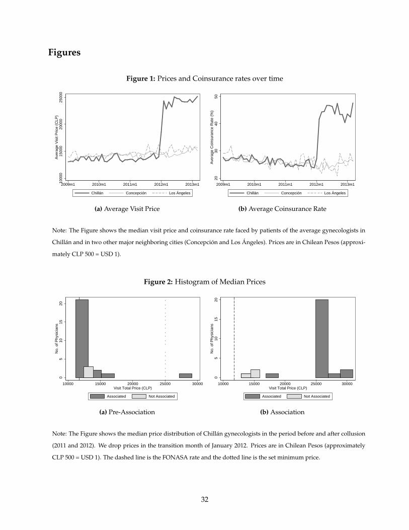
Figure 1 shows the evolution over time of the list price (before reimbursement) and coinsur-

ance rate for the average gynecologist-insurer pair in Chillan as well as in two of its main neigh-

boring cities. Panel (a) shows that the list price in Chillan increased by 75 percent when the Asso-

ciation formed, from roughly CLP 13,900 in December 2011 to CLP 24,300 in February of 2012. The

termination meant not only that the physicians rose their rates, but also that these rates would be

covered as out-of-network visits. Panel (b) shows an average increase of 68 percent on the average

coinsurance rate, from 25 percent to 42 percent. Combined, the out-of-pocket cost of a visit to the

average doctor in Chillan increased by almost 200%. There were no discernible changes in the

out-of-pocket costs in neighboring cities. 24,25

[INSERT FIGURE 1 HERE]

Compliance within the Association with the minimum visit price was substantial. Figure 2

shows a histogram of each physician’s median list price in 2011 and 2012. The dashed line shows

the FONASA rate and the dotted line indicates the minimum price set by the Association. The

price distribution shifts right in 2012, to the extent that the mode price in 2012 was almost twice as

high as the mode price in 2011. That was the case even for the most expensive doctors, who more

than doubled their list price. In addition, as we show in Section 4, those physicians who did not

raise their rates greatly increased their market share.26


small Isapre (closed to public enrollment), reached an agreement with the association in January 2012 of CLP 20,000 forvisits and 4.4 times the FONASA rate for surgeries.

24Table A1 shows the result of estimating a differences in differences model for prices and coinsurance rates. Theestimated price increase is 60% and the estimated increase in the coinsurance rate is 61% of the baseline levels in Chillan.The difference between the increase we report in the text and the estimated effect in the differences-in-differences is dueto a slight upward trend in the prices in the control group.

25As we discuss in the next section, the list price and coinsurance increases were offset by a shift to physicians thatdid not raise fees. Patients were surprised of the change, which was reported in the local media (FNE, 2013, p.9)

26Anecdotally, one of the physicians who did not join the Association was the former government’s director of healthservices in Nuble and, according to our data, started working in Chillan’s private sector only in mid-2010.

9

3 Data

We use the two main data sources of the antitrust case. The first source is the insurance com-

panies’ administrative data. It includes visits and surgeries that were registered by the Isapres

between January 2009 and March 2013 for gynecologists operating in Chillan and its neighboring

provinces.27 Each record contains physician and medical establishment identifiers, a scrambled

patient identifier, patient’s province of residence, date, price, out-of-pocket expenditures, and a

procedural code. The second dataset contains the receipts issued by the indicted physicians for

2012. It includes patient and physician identifiers and the total amount payed. We use receipts

information because many patients did not process their reimbursement with the insurance com-

panies after doctors became out-of-network and hence their visits are not included in the first

dataset. These two datasets combined allow us to reconstruct the universe of visits to gynecol-

ogists in Chillan and its neighboring cities.28 Given that we estimate aggregate demand at the

insurer-physician-month triad, we calculate the price and coinsurance rate as their average over

the visits corresponding to each combination. There are 29 different physicians in the data. We

drop observations corresponding to two physicians with less than 200 combined visits. Hence,

there are 25 associated and 2 non-associated physicians in our final sample.29 Finally, we obtain

the physicians’ main address from the case documents (FNE, 2013).30

Figure 3 shows the evolution of prices and profits over time for associated and non-associated

physicians, as well as for the average doctor. The figure assumes that physicians’ marginal cost

is equal to the FONASA rate, an assumption that we discuss in more detail in Section 5.2. The

figure shows that concurrently with the price increase among associated physicians there was a

large decrease in their average number of visits, as well as a large increase in the average visits

among non-associated doctors.

The profits of associated and non-associated doctors were stable before the Association, and

similar across groups. However, profits changed drastically for both groups after the Association

27There is no entry or exit of doctors during the time period we study.28We cannot match the two datasets at the patient level. For the demand estimation, we assume that the visits in the

receipts database were reimbursed at the out-of-network coverage rate.29In addition, we drop the physician-month observations corresponding to four physicians in 2012 that are likely to

be the result of incorrect imputation. For example, in the case of one physician two months register 35% of all yearlyreceipts.

30For the physicians who were not indicted, we use local websites.

10

was formed. We find that collusive profits were on average 4 to 5 times larger than in the pre-

collusive period, both for associated and non-associated doctors.


Figure 4 shows the evolution of total insurer costs and out-of-pocket expenses (the sum of

which corresponds to physician’s revenues). The figures shows that higher physician revenues

came at the expense of higher costs for both patients and insurers. For insurers, this means that

the lower out-of-pocket coverage and any endogenous response in demand did not compensate

for the higher list price.


4 Demand

4.1 Descriptive Evidence on Physician Switching

We start by providing evidence of significant demand responses to the large price increases doc-

umented in Section 2.2. In particular, we show that the price increases among colluded doctors

lead to a significant shift of patients across doctors, especially from colluding doctors towards

non-colluding doctors.

We define a visit of patient p to doctor i to represent a “switch” whenever the doctor seen by

p in her previous visit was i′ 6= i. Panel (a) of Figure 5 shows switching rates (i.e. the share of

visits defined as a “switch”) over time for Nuble (the province where doctors colluded) and for a

set of nearby provinces that we use as “control” provinces.31 Panel (a) also shows that switching

rates in Nuble and control provinces had a parallel trend and were stable over time before the

agreement. However, switching rates increased in Nuble after February 2012 from 22 to 32 percent

while there was no discernible increase in the switching rates in the control provinces. Panel (b)

shows regression results of switching on a Nuble indicator for each quarter separately. The panel

31We use Concepcion and Biobıo as control provinces, although the results are robust to using a different subset ofprovinces in the region as a control group. See footnote 16 for details.

11

indicates that the difference between the two groups is statistically significant immediately after

the association implemented the price hikes.


We formalize the previous description by estimating a difference-in-differences model for

switching rates. Let wplt be equal to 1 if the visit by patient p to doctor i in province l and period

t corresponds to a switch, and 0 otherwise. We estimate, by OLS, the parameters of the following

equation:

wpilt = αt + βTl + γTl × A f tert + g(t) + εilt, (1)

where Tl is an indicator for Nuble and g(t) controls for calendar time. We are interested in γ, the

estimated effect of the collusion on switching rates in Nuble.

Table 1 shows the estimation results of Equation (1). Column (1) uses g(t) = δA f tert, where

A f tert is dummy variable indicating post-Association dates. Column (2) replaces δA f tert by a full

set of year-month fixed effects. In both specifications we find γ = 0.07; a 7 p.p. increase in the

switching rate. This increase corresponds to a 32 percent of the baseline switching rate in Nuble

before the collusion. Appendix 5 shows that this large increase in switching across physicians

occurred mostly from colluding physicians towards non-colluding physicians.

[INSERT TABLE 1 HERE]

4.2 Demand Model

We model physicians as differentiated-product firms to allow for idiosyncratic preferences for

ob/gyns, which is likely an important feature of the industry. In our context, physicians are dif-

ferent from each other in terms of location, and possibly in terms of their quality, which introduces

both horizontal and vertical differentiation.

We assume a nested logit demand model, where the set of physicians is partitioned into non-

overlapping nests Bk, k = 1, . . . , K.32

32The nests are determined based on the doctor’s geographic location as explained in detail in Section 4.3. Usingnests captures differentiation across doctors arising from patient’s heterogeneous preferences for location.

12

The utility of patient p enrolled in insurer j for visiting doctor i in nest k in period t is

upijt = δijt + εijt + ηpkt + (1− σ)νpijt,

where δijt denotes the mean utility of insurees who visited doctor i at time t, εijt is the unobserved

mean-utility component of physician desirability, ηpkt is an unobserved common shock to physi-

cians in nest k, σ is a parameter that measures within nest correlation, and νpijt is an idiosyncratic

shock. The model assumes that ηpkt + (1− σ)νpijt has a generalized extreme value distribution.

The share of insurees who visit doctor i in time t (among all female insurees in insurance

company j), follows the standard share equation:

sijt =exp( δijt

1−σ )∑h∈Bk

[exp( δhjt

1−σ )]−σ

1 + ∑Kl=1 ∑h∈Bl

[exp( δhjt

1−σ )]1−σ

. (2)

We parameterize δijt as

δijt = αpijt(1− cijt) + µij + f (t), (3)

where pijt is the list price of a visit to physician i of enrollees of j in period t, 1− cijt is the coinsur-

ance rate, µij represent fixed effects for doctor-insurer pairs; and f (t) is a flexible function of time

that captures time-specific common shocks to demand.

4.3 Estimation

The estimation of Equation (2) poses three challenges. First, 26 percent of market-share observa-

tions in our data are equal to zero. This fact generates censoring in the estimation of Equation (2)

because the logit model does not allow for zero shares. Second, we need to specify the nesting

structure of the model. Finally, we face the standard endogeneity problem of prices and within

shares, as both εijt and the within shares are potentially correlated with prices. We address these

issues below.

Zero Shares As mentioned, many of the doctor shares in the data are zero. However, all doctors

are in all insurees’ choice set because insurees can in principle see any given doctor by paying the

13

corresponding out-of-pocket price (see Section 2). Therefore, the observed zero shares sijt can be

interpreted as the realization of small shares with a finite number of consumers, which differ from

the true population probabilities implied by the model.

We rely on Gandhi et al. (2014), who propose an asymptotic correction based on the assumption

that sales distribute according to Zipf’s Law.33 In that case, then for every insurer j

Mjsijt

1− s0jt|N, Mj, s0jt ∼ DCM

(θj1N , Mj(1− s0jt)

), (4)

where Mj is the market size (assumed to be equal to the number of female insurees in each Isapre),

N represents the number of doctors, and DCM(·) is the Dirichlet Multinomial Distribution with

the same N parameters θj and s0 represents the share of the outside option.

Denote the digamma function by ψ(·). We invert the shares equation, as in Berry (1994), and

take expectations to obtain:

ψ(θj + Mjsijt)− ψ(Mjs0jt) = αpijt(1− cijt) + µij + f (t)+

σ

[ψ(θj + Mjshjt)− ψ(∑

h∈kθj + Mjsijt)

]+ εijt,

(5)

which is a corrected version of the nested logit demand model that we can estimate. In this

equation, the left hand side corresponds to the expectation of the asymptotic dependent vari-

able of the nested logit model, E[ln(πijt/s0jt)

], where πijt denotes the true shares. The term in

square brackets is the expectation of the log asymptotic within share of physician i, E[ln πijt/Bk

]=

E[ln(πijt/ ∑h∈Bk

πiht)], j ∈ Bk. Our main objects of interest are the parameters α and σ.

Our estimation procedure has two steps. First, we estimate the DCM parameters θj of (4) via

Maximum Likelihood. Then, we use the resulting estimates to estimate the parameters of Equation

(5) using a 2-stage least squares estimator, that we discuss after we introduce the nesting structure

below.33Quan and Williams (2018) also implements the same correction.

14

Nesting Patients’ distaste for travel distance is a well-documented feature of demand for med-

ical services (see, e.g., Phelps and Newhouse, 1974). In the absence of data on patient’s location,

we use the nesting structure to accommodate for the fact that patients are more likely to substitute

to a physician that is either in the same medical center or has a practice in a nearby location. In

practice, we construct six nests based on the location of each doctor’s practice.

Figure A1 of the Appendix shows a map with the location of physicians and the resulting

nests. There are three large medical centers where five or more doctors co-locate. We assume

that each of those centers constitute a different nest. We group the rest of physicians—who either

are a single practice or are co-located with at most two others—into three other nests based on

geographic distance.34 Also, we construct two additional nests, one for physicians outside Chillan,

and another one for the outside option.

Endogeneity of Prices and Shares The estimation of Equation (5) by ordinary least squares

(OLS) will result in biased estimates in the presence of correlation between the price and within

share variables and the unobserved demand shocks εijt, as is also the case in the standard nested

logit model. We identify the own- and cross-price demand elasticities using the large increase in

out-of-pocket expenditures that stemmed from the gynecologists’ contract termination. In partic-

ular, we assume that the emergence and the membership in the Association was not a result of

idiosyncratic demand shocks, after controlling for the fixed effects.

Two pieces of evidence support this assumption. First, as shown in Figure 1, prices and coin-

surance rates in Chillan had a similar level and followed a similar trend to those in neighboring

cities before the Association emerged in Chillan. Thus, the data suggests that the emergence of the

Association in Chillan was not a result of particular conditions in this market. In particular it does

not seem that doctor’s bargaining position vis-a-vis insurance companies was substantially lower

in Chillan than in other neighboring cities.

Moreover, Figure 3 shows that profits and visits followed a similar trend in the pre-Association

period for associated and non-associated doctors. Therefore, the data shows that the membership

in the Association does not seem to have been driven by doctor-specific shocks to demand.

34Prices in the two types of groups are similar.For instance, the median (mean) price in the pre-Association periodwas 13,000 (13,226) and 13,044 (14,459) in these small and large practices, respectively.

15

Under this assumption, the Association period serves as an instrumental variable (IV) that

we use to solve the endogeneity problem. In particular, we use as instruments an indicator for

the post-agreement period (after February 2012) and its interaction with a dummy variable for

whether physician i joined the agreement.35 Hence, we identify the elasticities using changes in

prices and coinsurance rates within the doctor-insurer pair before and after the price change.36

4.4 Demand Estimation Results

Table 2 presents the results of estimating demand. All specifications use a month-of-the-year fixed

effect to control for seasonality and year fixed effects to allow for common trends. We present first

the OLS and IV results in Columns (1) and (2) of a simpler logit model estimated from Equation

(5) under the constraint σ = 0. Columns (3) and (4) present the OLS and IV nested logit estimation

results of Equation (5).37

In our main specification (Column (4) of Table 2) we find α = −0.050(0.018) and σ = 0.735(0.152).38

The Anderson-Rubin and Angrist and Pischke (2008) F-tests reject that the instruments are weak.

The rows under the estimates show the average own elasticity in the period before and after the

Association was formed.39

[INSERT TABLE 2 HERE]35Given that the association period, which we use as an instrument, has significant overlap with the 2012 year fixed

effect, we also tried fixed effects for 8 month periods. The results are unchanged.36Our instruments use a supply-side event to identify the demand as in Porter (1983), Eizenberg and Salvo (2015),

and Ale Chilet (2017).37Appendix A3 presents additional demand estimates resulting from standard ways of correcting for zero market

shares, like dropping observations with no sales or replacing the zeros with an arbitrary positive number. See Gandhiet al. (2014) for a discussion on the drawbacks of those methods.

38The estimate σ ∈ [0, 1], is consistent with utility maximization.39Note that the own elasticity for the logit and nested logit models are quite similar; yet, as expected, there is a large

difference in the cross elasticities (not reported).

16

5 The Association’s Pricing Strategy

5.1 Model

We model physicians during the Association period as differentiated-product firms, which may

or may not collude with their competitors.40 This allows us to calculate competitive and collusive

prices given the demand estimates.

In every period each of the Nc colluding physicians decides a unique list price for all insurance

companies. Colluding physicians take as given the prices of the N − Nc non-colluding physicians

—which are set non-strategically at their pre-agreement level— and the out-of-network coinsur-

ance rates for each insurer. We denote by pN the vector with the stacked prices of all the colluding

physicians, cj the vector of stacked coverage rates (1 minus coinsurance rates) in insurer j and the

corresponding vector of monthly visits qj(pN, cj). The first-order condition of colluding physi-

cians can be written in matrix form for each period as

pN = mc−

Ω∗ ∗∑j

Ej ∗ Cj

−1

∑j

qj(p, cj), (6)

where the operator ∗ denotes element-by-element multiplication.41 The matrix Ej corresponds to

the own- and cross-derivatives of demand with respect to out-of-pocket prices in insurer j, which

we estimated in Section 4. The matrix Cj represents coinsurance rates, with elements Cj(i, s) =

1− cij, that converts the list prices into out-of-pocket prices for visits to doctor i among insurees

of Isapre j. Finally, the vector mc is the physicians’ marginal cost. We assume that mc is constant

across physicians, and is equal to the FONASA rate, which is determined yearly by the regulator.

The rationale for this assumption is that the FONASA rate corresponds to the opportunity cost of

seeing one extra privately insured patient.42

We also define the ownership matrix Ω∗ for the colluding physicians. The ownership ma-

40We do not model bargaining with the insurers during the agreement period because physicians terminated theircontracts with the insurers.

41We omit time indexes to simplify notation.42We are making the implicit assumption that doctors can always substitute a private patient for a public patient.

This assumption is justified by the well-documented lack of specialist doctors and long waiting times in the publicsystem. As an example, in 2017 there were almost 70 thousand individuals nationwide on the waiting list to visit anob/gyn, among which almost 50 thousand had been waiting more than 4 months (INDH, 2018).

17

trix specifies the degree to which each colluding physician internalizes other physicians’ profits.

As in Nevo (1998) we focus on a general ownership matrix to accommodate different degrees of

coordination on prices among colluding physicians, parametrized with a scalar κ ∈ [0, 1] such that

Ω∗ =

1 κ . . . κ

κ 1 . . . κ

......

. . ....

κ κ . . . 1

. (7)

When κ = 0, the matrix Ω∗ becomes the identity matrix, which determines the Nash equilibrium;

any κ > 0 determines a different partial collusive equilibrium, with a higher κ indicating a higher

degree of coordination on prices. The extreme of κ = 1 corresponds to full collusion on prices.43

For any given assumed value of κ, we solve for pN by numerically finding the fixed point in

Equation (6).

Capacity Constraints Physicians see a mix of patients that are either privately or publicly in-

sured. Our supply and demand models assume that capacity constraints for visits of privately-

insured patients do not bind – so that physicians can always see an extra private patient at the

expense of not seeing a public patient. Binding capacity constraints in the data would imply that

we underestimate the price coefficient in the demand model. Moreover, binding capacity con-

straints could generate corner solutions in the supply model, and reduce the potential deviation

profits in the counterfactuals we study below (Staiger and Wolak, 1992).We provide evidence sup-

porting the absence of binding capacity constraints for private visits, both in the data and in the

predictions of the model, in Appendix A6.

5.2 Results

The main results of the predicted price from Equation (6) are in Figure 6. The figure presents the

time series of equilibrium prices assuming Nash-Bertrand competition among associated doctors

43We refer to Miller and Weinberg (2017) for the discussion of whether κ can be interpreted as a conduct parameter.See the references there, especially Corts (1999) and Sullivan (2017).

18

(κ = 0).44 We plot (quantity-weighted) average Nash prices, as well as the 25 and 75 percentiles

of the distribution of prices across colluding physicians. For comparison, the figure also includes

the average observed prices, the marginal cost (the FONASA rate), and the minimum price set by

the Association (CLP 25,000). In addition, Figure 7 shows the distribution of average Nash prices

of each physician during the Association period.



Three facts about our results are particularly noteworthy. First, as shown in Figure 6, the

average Nash-Bertrand price (CLP 26,800) is almost twice as high as the observed price in the

pre-agreement period. This difference reflects the low bargaining power of the doctors vis-a-vis

insurance companies in the pre-Association period.

Figure 6 also shows that the average Nash-Bertrand price is almost equal to average price set

by the members of the Association. By contrast, the collusive price (when κ = 1) is equal to CLP

52,336; twice as high as the average observed price. Panel (a) of Figure 8 shows the ratio between

the (quantity-weighted) average predicted price and (quantity-weighted) average observed price.

Also, κ = 0 minimizes the difference between the prices predicted by the supply model and the

true prices. Panel (b) of Figure 8 shows the (quantity-weighted) average of absolute differences

between the predicted and observed prices is increasing in κ, formally defined as

f (κ) ≡ 1T ∑

t≥t0

1N ∑i |1−

PNit (κ)Pit|qijt(κ)

∑i qijt (κ),

where t0 is the date when the Association was formed, T is the number of months post-association.

Pit is the observed price and PNit (κ) and qijt(κ) are the predicted prices and quantities as a function

of κ. As shown in Panel (b) of Figure 8, f (κ) is increasing in κ so that the no-coordination solution

provides the best fit to the data.45

44Because doctors left the network, we use out-of-network coinsurance rates, which we calculate as the averagecoinsurance rate of each insurer-physician pair across out-of-network visits in the Association period.

45 f (0) = 0.17%, i.e., our prediction error is approximately 17 percent of the actual price.

19

Third, as shown in Figure 7, the distribution of Nash-Bertrand prices is such that the minimum

price barely binds.


Our empirical results provide two main insights. First, the Association served as a collu-

sive device on the physicians’ decision to become out-of-network providers, but not to set supra-

competitive prices. Thus, the price increase during collusion stems from the fact that the physicians

were no longer constrained by their previous agreements with the insurers. Second, our findings

allow us to assess the role of the minimum price as an effective collusive mechanism. In partic-

ular, Harrington (2016) shows that the use of a minimum price is an incentive compatible way

of achieving supra-competitive prices for heterogeneous firms. Yet, our results show that the level

chosen for the minimum price was not binding in the Nash equilibrium. Therefore, the minimum

price was not helpful to raise profits above competitive levels. Hence, we interpret the use of a

minimum price as a focal price, which helped doctors coordinate into switching to the competitive

equilibrium.

Robustness to the marginal cost assumption An important assumption in our empirical analy-

sis is the level of the marginal cost, which we assumed to be equal to the FONASA rate. However,

one could argue that a visit of a privately insured patient is more costly than a visit of a publicly in-

sured patient if, for instance, doctors spend more time with the privately-insured patients. In that

case, the FONASA rate (CLP 10, 970) would correspond to a lower bound for the marginal cost. On

the other hand, the actual pre-agreement price (CLP 13, 982) is an upper bound on the marginal

cost, as a higher marginal cost would violate doctors’ participation constraint in the agreement

with insurers. In the extreme case that the pre-agreement price was equal to the doctor’s marginal

cost —a situation in which the pre-association price leaves doctors just indifferent between partic-

ipating in the market or not— we would underestimate the equilibrium prices by CLP 3, 000. Still,

the conclusion about lack of price coordination is unaffected by assuming a higher marginal cost.

20

5.3 Stability of the Association

In this subsection we evaluate the stability of the Association by analyzing whether colluding

physicians would have profited from leaving the Association unilaterally. In fact, insurers ap-

proached physicians individually during the Association period and offered them to rejoin their

network. Yet, the Association prevailed and no physician deviated. Finding a large number of

physicians with positive deviation profits would entail that the Association was not stable or de-

pended critically on non-monetary incentives. On the contrary, finding negative deviation profits

provides support to our model as a characterization of a stable collusive agreement.

We evaluate the decision to stay in the Association under the assumption that prices out-of-

network are set in the Nash-Bertrand game, which is consistent with our findings in the previous

section. We assume that deviating physicians set their price at their pre-Association average, that

is, we assume they return to their original insurer contract.

Formally, for a set S of doctors in the Association, the vector of prices p(S) has element i

defined by:

pi(S) =

pd

i , if i /∈ S

pNi , if i ∈ S

where pNi is the ith element of the vector defined implicitly by Equation 6 for doctors in S , and pd

i

is the average of in-network prices of doctor i.

Similarly, the vector of coinsurance rates (cj) has element i defined by:

ci,j(S) =

cI

i,j, if i /∈ S

cOi,j, if i ∈ S

where cIi,j an cO

i,j denote the in-network and out-of-network coinsurance rates, respectively

The profits for physician i under S depends on physician i’s price and coinsurance rate as well

21

as all other physician’s prices and coinsurance rates, denoted by p−i(S) and c−i(S);

πi(S) = ∑j

(pi(S)−mc

)qj

(pi(S), p−i(S), ci,j(S), c−i,j (S)

).

When physician i deviates from the Association her deviation profits are

πi(S \ i

)− π (S) = ∑

j

(pd

i −mc)

qj

(pN

i , p−i (S) , cIi,j, c−i,j (S)

)−∑

j

(pN

i −mc)

qj

(pd

i , p−i (S) , cOi,j, c−i,j (S)

)(8)

When i deviates, she lowers the price from pNi to pd

i , but also profits from a higher coverage

rate for her patients. These two effects can be decomposed by re-writing equation (8) as

πi(S \ i

)− πi (S) =

∑j

(pd

i −mc)

qj

(pd


)−∑

j

(pN

i −mc)

qj

(pN


)+ ∑

j

(pd

i −mc)(

qj

(pd


)− qj

(pd

i , p−i (S) , c0i,j, c−i,j (S)

))(9)

The first term of equation (9) is the change in profits due to price deviation while keeping

coverage rates at the out-of-network level. As prices are set at the Nash-Bertrand level for out-of-

network coverage, the first term in equation (9) is negative. On the other hand, the second term

is the deviation towards being outside of the network. This term is positive, and proportional to

the extra visits generated by higher coverage in-network.46 Therefore, deviation profits have an

ambiguous sign, so we quantify them empirically using our demand estimates.


Panel (a) of Figure 9 presents the results. The panel shows the histogram of deviation profits

46It is easy to show that qj

(pd


)− qj

(pd

i , p−i (S) , c0i,j, c−i,j (S)

)' −Eij × pd

i ×(

cIi,j − cO

i,j

)> 0

where Eij is the own-price elasticity of demand for doctor i among enrollees of j with respect to the out-of-pocket price.

22

across physicians, calculated as a share of the collusive profits,(πi(S)− πi(S \ i)

)/πi(S). Each

unit of observation corresponds to a different deviating physician (and, therefore, to a different

counterfactual scenario) among the 25 colluding physicians in our sample.

We find positive deviation profits for only one of the 25 colluding physicians. The median

doctor would have lost 79 percent of her collusion profits by deviating to their pre-agreement

price and staying in-network.

In order to assess the overall stability of the Association, we iterate this process by removing

the doctor with positive deviation profits and recalculating the new equilibrium prices and profits

from unilateral deviations until no doctors have positive deviation profits. This process stops

in the second iteration, in the counterfactual situation where the doctor with positive deviations

profits leave the Association as it was actually formed. Panel (b) o Figure 9 shows the distribution

of deviation profits after the doctor with positive deviation profits in Panel (a) deviates. In this

case, none of the remaining doctors have incentives to deviate.

These findings provide evidence of the incentive compatibility of the Association’s collusive

strategy. This strategy not only prevented deviations in prices while out-of-network, but it also

prevented deviations with respect to the decision to leave the insurers’ network.

Incentives to join the Association An alternative interpretation of equation (9) is that it quanti-

fies physician i’s incentives to join the Association under the assumption that everyone else joins

and charges prices p−i (S). However, it might be natural to assume that each physician considers

her impact on the equilibrium premiums when considering whether to join the Association or not.

In that case, each physician i computes her profits from not joining, π(S \ i

), that depend on the

outcome of the Nash-Bertrand pricing game when physician i does not join, p−i(S \ i

).

We show the resulting deviation profits after considering endogenous repricing of the associ-

ated physicians in Appendix A7 . We find that price adjustments are small so that deviation profits

in this case are similar to the results of Figure 9. We interpret this finding as showing that joining

the Association was incentive compatible.

23

5.4 The role of coordination

In this section we calculate every doctor’s profits in the counterfactual scenario where she would

have unilaterally left the network. In this exercise, the focal doctor i sets her visit price according

to the first order condition in Equation (6), while the others keep their prices at their individual

pre-agreement average. In terms of the notation introduced in Section 5.3, this results in profits

πi(i) for the focal doctor who leaves the network unilaterally. We calculate deviation profits

relative to πi(∅), i.e., the profits in the case were no doctor leaves the network.

Figure 10 plots the relative profits for every doctor from unilaterally becoming out-of-networkπi(i)−π(∅)

π(∅), as well as the relative profits from jointly becoming out-of-network as in the Association

πi(S)−π(∅)π(∅)

.


The figure shows that most physicians would have had higher profits from leaving the net-

work and setting their optimal price (assuming that all other doctors would have stayed in the

network) relative to staying in-network. However, for several physicians the gains from deviating

were small. In fact, one third of physicians would have increased their profits by less than 10 per-

cent by deviating unilaterally. The figure also shows that the Association provides much higher

profits than the in-network status-quo or than unilateral deviations for every doctor. On average,

joint deviation produced profits 400 percent higher than the status quo, and 140 percent higher

profits than unilateral deviation.

Two main insights emerge from this result. The fact that doctors did not leave the network

unilaterally is consistent with the case documents showing that the physicians’ goal was to reach

ultimately better terms with the insurers, and that coordinated action was used to increase their

bargaining position. In turn, coordinated action raised their outside option to the point where the

negotiation broke down. The facts that unilateral deviations did not occur despite being incentive

compatible, and that coordination entailed higher profits suggest that communication played an

important role in the breakdown of negotiations.

24

6 Conclusion

Collusion among a large number of agents through a trade association is a common phenomenon.

In this paper we study the collusive strategies of a trade association of physicians in the context of

a vertical negotiation with payers. The case closely mirror several cases challenged by the FTC, in

spite of recent calls by practitioners that put into question the prosecution of agreements that seek

to counteract large imbalances of power in negotiations. The Association members undertook

two coordinating strategies: joint termination of their contracts with insurance companies and

agreement on a minimum price per visit. These joint measures were effective in increasing the

members’ profits. We find that the realized prices coincided with the competitive price and that

the minimum price was barely binding. These findings suggest that the change in the structure of

the physician-insurer relationship was more important to increase physicians’ profits than price

coordination.

The counterfactual exercises allow us to understand the stability and the coordination role

of the association. First, we find that unilateral deviation profits from joint contract termination

are much lower than the collusive profits. This result indicates that the Association’s collusive

strategy was incentive compatible. Second, we find that physicians would have benefited from

leaving insurers unilaterally, but that they benefited much more from leaving insurers jointly. The

fact that, in reality, physicians left insurers jointly is consistent with the physicians wanting to

reach ultimately better terms with the insurers and with coordinated action being used to increase

their bargaining position vis-a-vis the insurers. These results suggest that coordination played a

key role in the price increases of 2012.

Our work has antitrust implications. Some antitrust practitioners have argued that small

downstream firms should be allowed to jointly negotiate with larger upstream firms in order to

“countervail market power,” as most of the surplus is extracted by the large firm. We show that

in the case we study joint negotiation caused large price hikes to consumers. This finding pro-

vides empirical support to the claim that such joint negotiations should be disallowed when the

policymaker’s goal is to maximize consumer surplus.

In addition, the Gynecologists’ Association did not manage to raise prices much above the

25

competitive outcome despite sustained coordination. However, the Association was highly suc-

cessful in coordinating the bargaining efforts vis-a-vis the insurers. This result suggests that the

nature of coordination in negotiations in vertical relationships is different from that of coordina-

tion in prices. While it is well known that price collusion among a large number of heterogeneous

agents is difficult, the case studied in this paper suggests that such hurdles might not arise in other

types of coordination.

Furthermore, the case studied in our paper highlights the role of communication through a

trade association in cases of successful coordination. Although the presence of communication is

central in antitrust practice, its role in collusion is not well understood by theoretical models.

Finally, the failed negotiation documented in this paper constitutes a departure from the agree-

ment equilibria usually studied in the empirical industrial organization literature. We interpret

our findings as showing that the Association increased the profits of doctors’ outside option in the

bargaining game so that there was no longer surplus created by the agreement with insurers. This

fact ultimately resulted in a breakdown of the physician-insurers negotiation. Documenting such

breakdowns is important because they shed light on the outside options of each side, and pro-

vide theoretical support for the modeling of equilibrium bargaining outcomes. Understanding

the dynamics of a failed bargaining process is a promising area for future research.

26

References

ACCC (2018). Potential ACCC class exemption for collective bargaining. Australian Competition

and Consumer Commission. Discussion Paper.

ALE CHILET, J. (2017). Gradually rebuilding a relationship: The emergence of collusion in retail

pharmacies in Chile. Working Paper.

ANGRIST, J. D. and PISCHKE, J.-S. (2008). Mostly harmless econometrics: An empiricist’s companion.

Princeton University Press.

ASHENFELTER, O. and JOHNSON, G. (1969). Bargaining theory, trade unions, and industrial strike

activity. American Economic Review.

ASKER, J. (2010). A study of the internal organization of a bidding cartel. American Economic Re-

view, 100 (3), 724–62.

ASSOCIATION, A. M. (2011). Competition in health insurance: A comprehensive study of u.s.

markets, 2017 update. Technical report, American Medical Association, Chicago, IL.

ATHEY, S. and BAGWELL, K. (2001). Optimal collusion with private information. RAND Journal of

Economics, pp. 428–465.

— and — (2008). Collusion with persistent cost shocks. Econometrica, 76 (3), 493–540.

—, — and SANCHIRICO, C. (2004). Collusion and price rigidity. The Review of Economic Studies,

71 (2), 317–349.

AUSTIN, D. R. and BAKER, L. C. (2015). Less physician practice competition is associated with

higher prices paid for common procedures. Health Affairs, 34 (10), 1753–1760.

BAKER, J. B., FARRELL, J. and SHAPIRO, C. (2008). Merger to monopoly to serve a single buyer:

Comment. Antitrust LJ, 75, 637.

BAKER, L. C., BUNDORF, M. K., ROYALTY, A. B. and LEVIN, Z. (2014). Physician practice compe-

tition and prices paid by private insurers for office visits. Jama, 312 (16), 1653–1662.

BERRY, S. T. (1994). Estimating discrete-choice models of product differentiation. The RAND Jour-

nal of Economics, pp. 242–262.

BINGAMAN, A. (1996). Recent enforemcent actions by the antritrust division against trade associ-

ations. 32nd Annual Symposium of the Trade Association and Antitrust Law Committee of the

Bar Association of the District of Columbia, US Department of Justice, Antitrust Division.

27

BITRAN, E., ESCOBAR, L. and GASSIBE, P. (2010). After Chile’s health reform: Increase in coverage

and access, decline in hospitalization and death rates. Health Affairs, 29 (12), 2161–2170.

BLAIR, R. D. and DEPASQUALE, C. (2011). Considerations of countervailing power. Review of

Industrial Organization, 39 (1-2), 137.

— and HERNDON, J. B. (2004). Physician cooperative bargaining ventures: An economic analysis.

Antitrust Law Journal, 71 (3), 989–1016.

BRESNAHAN, T. F. (1987). Competition and collusion in the American automobile industry: The

1955 price war. The Journal of Industrial Economics, pp. 457–482.

CAMPBELL, T. (2007). Bilateral monopoly in mergers. Antitrust Law Journal, 74 (3), 521–536.

— (2008). Bilateral monopoly: Further comment. Antitrust LJ, 75, 647.

CARD, D. (1990). Strikes and wages: a test of an asymmetric information model. The Quarterly

Journal of Economics, 105 (3), 625–659.

CARNEVALI, F. (2011). Social capital and trade associations in america, c. 1860–1914: a microhis-

tory approach. The Economic History Review, 64 (3), 905–928.

CILIBERTO, F. and WILLIAMS, J. W. (2014). Does multimarket contact facilitate tacit collusion?

Inference on conduct parameters in the airline industry. The RAND Journal of Economics, 45 (4),

764–791.

CLARK, R. and HOUDE, J.-F. (2013). Collusion with asymmetric retailers: Evidence from a gaso-

line price-fixing case. American Economic Journal: Microeconomics, 5 (3), 97–123.

COMPETITION COMMISSION OF SINGAPORE (2009). Ccs fines 16 coach operators and association

uss 1.69 million for price-fixing. Press Release.

CORTS, K. S. (1999). Conduct parameters and the measurement of market power. Journal of Econo-

metrics, 88 (2), 227–250.

CRAMTON, P. and TRACY, J. (2003). Unions, bargaining and strikes. In International Handbook of

Trade and Unions, Edward Elgar.

DOJ and FTC (2011). Statement of antitrust enforcement policy regarding accountable care organi-

zations participating in the medicare shared savings program; notice, part ii. Federal Registrer.

DONOVAN, W. J. (1926). The legality of trade associations. Proceedings of the Academy of Political

Science in the City of New York, 11 (4), 19–26.

28

DUNN, A. and SHAPIRO, A. H. (2014). Do physicians possess market power? The Journal of Law

Economics, 57 (1), 159–193.

EIZENBERG, A. and SALVO, A. (2015). The rise of fringe competitors in the wake of an emerging

middle class: An empirical analysis. American Economic Journal: Applied Economics, 7 (3), 85–122.

FNE (2013). Requerimiento. Rol C No. 265-13.

— (2014). Observaciones a la prueba. Rol C No. 265-13.

FTC (2018). Spotlight on trade associations. https://www.ftc.gov/tips-advice/

competition-guidance/guide-antitrust-laws/dealings-competitors/

spotlight-trade, accessed: 2018-06-30.

FULTON, B. D. (2017). Health care market concentration trends in the united states: evidence and

policy responses. Health Affairs, 36 (9), 1530–1538.

GANDHI, A., LU, Z. and SHI, X. (2014). Demand estimation with scanner data: Revisiting the

loss-leader hypothesis. Working Paper.

GENESOVE, D. and MULLIN, W. P. (1998). Testing static oligopoly models: conduct and cost in

the sugar industry, 1890-1914. The RAND Journal of Economics, pp. 355–377.

— and — (2001). Rules, communication, and collusion: Narrative evidence from the sugar insti-

tute case. American Economic Review, 91 (3), 379–398.

GOWRISANKARAN, G., NEVO, A. and TOWN, R. (2015). Mergers when prices are negotiated:

Evidence from the hospital industry. American Economic Review, 105 (1), 172–203.

GU, W. and KUHN, P. (1998). A theory of holdouts in wage bargaining. American Economic Review,

pp. 428–449.

HARRINGTON, J. E. (2016). Heterogeneous firms can always collude on a minimum price. Eco-

nomics Letters, 138, 46–49.

— and SKRZYPACZ, A. (2011). Private monitoring and communication in cartels: Explaining re-

cent collusive practices. American Economic Review, 101 (6), 2425–49.

HICKS, J. (1932). The Theory of Wages. New York: Macmillan.

HO, K. and LEE, R. S. (2017). Insurer competition in health care markets. Econometrica, 85 (2),

379–417.

IBANEZ, C. (2017). Caracterizacion del mercado de seguros complementarios de salud en base a

encuesta casen 2015. Documento de Trabajo, Superintendencia de Salud.

29

https://www.ftc.gov/tips-advice/competition-guidance/guide-antitrust-laws/dealings-competitors/spotlight-trade



IGAMI, M. and SUGAYA, T. (2017). Measuring the incentive to collude: The vitamin cartels, 1990-

1999, working Paper.

INDH (2018). Informe anual 2018: Situacion de los derechos humanos en chile. https://

bibliotecadigital.indh.cl/handle/123456789/1173, accessed: 2019-07-24.

KENNAN, J. (1986). The economics of strikes. Handbook of labor economics, 2, 1091–1137.

KIRBY, A. J. (1988). Trade associations as information exchange mechanisms. The RAND Journal of

Economics, pp. 138–146.

KUHN, K.-U., MATUTES, C. and MOLDOVANU, B. (2001). Fighting collusion by regulating com-

munication between firms. Economic Policy, 16 (32), 169–204.

LEE, R. S. and FONG, K. (2013). Markov perfect network formation: An applied framework for

bilateral oligopoly and bargaining in buyer-seller networks. Working Paper.

LEVENSTEIN, M. C. (1997). Price wars and the stability of collusion: A study of the pre-World War

I bromine industry. The Journal of Industrial Economics, 45 (2), 117–137.

— and SUSLOW, V. Y. (2006). What determines cartel success? Journal of economic literature, 44 (1),

43–95.

— and — (2011). Breaking up is hard to do: Determinants of cartel duration. Journal of Law &

Economics, 54, 455–462.

MCGAHAN, A. M. (1995). Cooperation in prices and capacities: Trade associations in brewing

after repeal. The Journal of Law and Economics, 38 (2), 521–559.

MEIER, M., ALBERT, B. and MONAHAN, K. (2017). Overview of ftc actions in health care ser-

vices and products. Available at https://www.ftc.gov/system/files/attachments/

competition-policy-guidance/overview_health_care_august_2018.pdf.

MILLER, N. H. and WEINBERG, M. C. (2017). Understanding the price effects of the MillerCoors

joint venture. Econometrica, 85 (6), 1763–1791.

MOTTA, M. (2004). Competition Policy: Theory and Practice. Cambridge University Press.

MULLAN, H. and TIMAN, N. (2018). Strengthening buyer power as a solution to platform market

power. Competition Policy International. Antitrust Chronicle, (9).

NEVO, A. (1998). Identification of the oligopoly solution concept in a differentiated-products in-

dustry. Economics Letters, 59 (3), 391–395.

30

https://bibliotecadigital.indh.cl/handle/123456789/1173

https://bibliotecadigital.indh.cl/handle/123456789/1173

https://www.ftc.gov/system/files/attachments/competition-policy-guidance/overview_health_care_august_2018.pdf

https://www.ftc.gov/system/files/attachments/competition-policy-guidance/overview_health_care_august_2018.pdf

— (2001). Measuring market power in the ready-to-eat cereal industry. Econometrica, 69 (2), 307–

342.

OECD (2007). Potential pro-competitive and anti-competitive aspects of trade/business associa-

tions.

OLIPHANT, H. (1926). Trade associations and the law. Columbia Law Review, 26, 381.

PHELPS, C. E. and NEWHOUSE, J. P. (1974). Coinsurance, the price of time, and the demand for

medical services. the Review of Economics and Statistics, pp. 334–342.

PORTER, R. H. (1983). A study of cartel stability: the Joint Executive Committee, 1880-1886. The

Bell Journal of Economics, pp. 301–314.

QUAN, T. W. and WILLIAMS, K. R. (2018). Product variety, across-market demand heterogeneity,

and the value of online retail. The RAND Journal of Economics, 49 (4), 877–913.

ROLLER, L.-H. and STEEN, F. (2006). On the workings of a cartel: Evidence from the norwegian

cement industry. American Economic Review, 96 (1), 321–338.

STAIGER, R. W. and WOLAK, F. A. (1992). Collusive pricing with capacity constraints in the pres-

ence of demand uncertainty. The RAND Journal of Economics, pp. 203–220.

SULLIVAN, C. (2017). The ice cream split: Empirically distinguishing price and product space

collusion, working Paper.

SYMEONIDIS, G. (2002). The effects of competition: Cartel policy and the evolution of strategy and struc-

ture in British industry. MIT press.

VIVES, X. (1990). Trade association disclosure rules, incentives to share information, and welfare.

the RAND Journal of Economics, pp. 409–430.

WHINSTON, M. D. (2008). Lectures on Antitrust Economics. The Cairoli Lectures.

31

Figures

Figure 1: Prices and Coinsurance rates over time

1000

015

000

2000

025

000

Ave

rage

Vis

it P

rice

(CLP

)

2009m1 2010m1 2011m1 2012m1 2013m1

Chillán Concepción Los Ángeles

(a) Average Visit Price20

3040

50A

vera

ge C

oins

uran

ce R

ate

(%)

2009m1 2010m1 2011m1 2012m1 2013m1

Chillán Concepción Los Ángeles

(b) Average Coinsurance Rate

Note: The Figure shows the median visit price and coinsurance rate faced by patients of the average gynecologists in

Chillan and in two other major neighboring cities (Concepcion and Los Angeles). Prices are in Chilean Pesos (approxi-

mately CLP 500 = USD 1).

Figure 2: Histogram of Median Prices

05

1015

20N

o. o

f Phy

sici

ans

10000 15000 20000 25000 30000Visit Total Price (CLP)

Associated Not Associated

(a) Pre-Association

05

1015

20N

o. o

f Phy

sici

ans

10000 15000 20000 25000 30000Visit Total Price (CLP)


(b) Association

Note: The Figure shows the median price distribution of Chillan gynecologists in the period before and after collusion

(2011 and 2012). We drop prices in the transition month of January 2012. Prices are in Chilean Pesos (approximately

CLP 500 = USD 1). The dashed line is the FONASA rate and the dotted line is the set minimum price.

32

Figure 3: Monthly Average Number of Visits and Profits over Time

050

100

150

200

250

Prof

its (C

LP '0

00)

025

5075

100

125

Visi

ts

2009m1 2010m1 2011m1 2012m1 2013m1

Visit - Not Associated Profits - Not AssociatedVisits - Associated Profits - AssociatedVisits - All Profits - All

Note: The Figure shows the average number of visits and profits (using the FONASA payment as the cost) for all

doctors combined and for groups of associated and not associated physicians.

33

Figure 4: Insurer Expenses and Out-of-Pocket Expenses

02

46

8C

LP M

illion

2009 2010 2011 2012 2013

Insurer Expenses Out-of-Pocket Expenses

Note: The Figure shows patients’ and insurers’ aggregated expenses of visits.

The sum of the two lines represent physicians’ revenues.

34

Figure 5: Physician switching rates in Nuble and surrounding provinces.1

.2.3

.4Sw

itchi

ng ra

te

2011m1 2011m7 2012m1 2012m7 2013m1

Nuble Control Provinces

(a) Switching Rates

0.0

5.1

.15

.2.2

5Es

tima

te

2011m1 2011m7 2012m1 2012m7 2013m1

(b) Difference

Note: Panel (a) shows the average switching rates across doctors for OBGyN visits in the province of Nuble

(where collusion occurred) and in surrounding provinces (Biobıo and Concepcion). Panel (b) shows the quarterly

difference in switching rates between the two groups and their 95 percent confidence intervals. The vertical line

marks the implementation date of the collusive measures. The horizontal line in Panel (b) shows the estimates

average in 2011.

35

Figure 6: Simulated and Actual Prices

1000

015

000

2000

025

000

3000

0Pr

ices

(CLP

)

2011m1 2011m7 2012m1 2012m7 2013m1

Nash Price Nash Price p25/p75Minimum Price FonasaActual Price

Note: The Figure shows the Nash prices for out-of-network coinsurance rates, the average actual price, and the

FONASA rate. The dashed line shows the minimum price set by the Association. In addition, the vertical lines show

the 25 and 75 percentiles of the out-of-network Nash prices, and the dot indicates the median.

36

Figure 7: Distribution of Nash-Bertrand Prices

05

1015

Freq

uenc

y

24000 26000 28000 30000 32000 34000Price (CLP)

Note: The Figure plots the histogram of the estimated Nash prices of each associated physician, averaged over the

Association period. The dashed line shows the Association’s minimum price.

Figure 8: Equilibrium Prices and Fit as a function of κ

1

1.2

1.4

1.6

1.8

2

Aver

age

Pred

icted

Pric

e/Av

erag

e O

bser

ved

Price

0 .1 .2 .3 .4 .5 .6 .7 .8 .9 1κ

(a) Predicted relative to observed

.2

.4

.6

.8

1

loss

func

tion

0 .1 .2 .3 .4 .5 .6 .7 .8 .9 1κ

(b) Absolute error (loss function)

Note: Panel (a) shows the ratio between the sales-weighted average price predicted by the supply model andthe sales-weighted average observed price in the post-association period. Panel (b) shows the “loss function”

f (κ) ≡ 1T ∑t≥t0

1N ∑i |1−

PNit (κ)

Pit|qijt(κ)

∑i qijt(κ),

37

Figure 9: Deviation Profits and Association Stability0

24

68

Fre

quen

cy

-1 -.5 0 .5 1deviation profit (%)

(a) Step 1

02

46

8F

requ

ency


(b) Step 2

The Figure shows the distribution of per-period deviation profits across physicians. Each point in the figure corre-

sponds to the deviation profit of a different physician, as a percentage of the profit from staying in the Association.

Figure 10: Deviation Profits as a Share of In-network Profits

05

1015

Dev

iatio

n P

rofit

[tim

es]

1 2 3 4 5 6 7 8 9 10 11 12 13 14 15 16 17 18 19 20 21 22 23 24 25

Unilateral Termination Joint Termination

Note: The Figure plots the gains from leaving the network under the assumption that all doctors of the Association

leave the network (Joint Termination) and under the assumption that only the focal doctor becomes out-of-network

(Unilateral Termination). Deviation profits are calculated as the difference in profits between each scenario and the

profits under the situation that all doctors stay in-network.

38

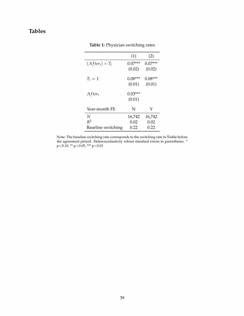
Tables

Table 1: Physician switching rates

(1) (2)

(A f tert)× Tl 0.07*** 0.07***(0.02) (0.02)

Tl = 1 0.08*** 0.08***(0.01) (0.01)

A f tert 0.03***(0.01)

Year-month FE N Y

N 16,742 16,742R2 0.02 0.02Baseline switching 0.22 0.22

Note: The baseline switching rate corresponds to the switching rate in Nuble beforethe agreement period. Heteroscedasticity robust standard errors in parentheses. *p<0.10, ** p<0.05, *** p<0.01

39

Table 2: Demand Estimates

(1) (2) (3) (4)

Logit OLS Logit IV NL OLS NL IV

pijt(1− cijt) 0.004 -0.146*** 0.004 -0.050***

(0.010) (0.017) (0.004) (0.018)

ln within-share 1.040*** 0.735***

(0.005) (0.152)

ηpre 0.02 -0.60 -0.29 -0.65

ηpost 0.04 -1.53 -0.75 -1.68

Observations 6620 6620 6620 6620

AR F-stat 39.42 39.42

AP F-stat 1 1899.99 334.84

AP F-stat 2 19.83

Note: The Table shows the demand estimates. All specifications include month-of-the-year and year fixed

effects. Out of pocket expenditures are in thousand CLP. The AR F-stat corresponds to the Anderson-Rubin

Wald F-statistic. The AP F-stat 1 and 2 correspond to the first-stage F statistics of the excluded instruments

for out-of-pocket expenditure and within shares respectively (Angrist and Pischke, 2008). Heteroscedastic-

ity robust standard errors in parentheses. * p<0.1, ** p<0.05, *** p<0.01

40

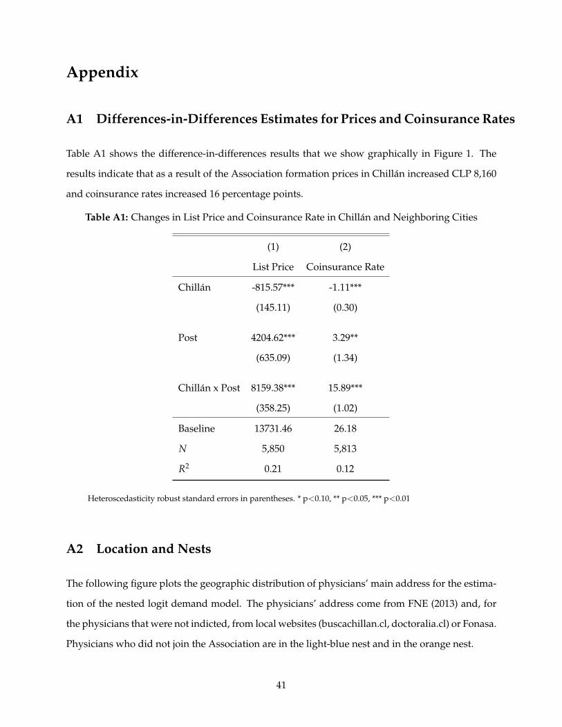
Appendix

A1 Differences-in-Differences Estimates for Prices and Coinsurance Rates

Table A1 shows the difference-in-differences results that we show graphically in Figure 1. The

results indicate that as a result of the Association formation prices in Chillan increased CLP 8,160

and coinsurance rates increased 16 percentage points.

Table A1: Changes in List Price and Coinsurance Rate in Chillan and Neighboring Cities

(1) (2)

List Price Coinsurance Rate

Chillan -815.57*** -1.11***

(145.11) (0.30)

Post 4204.62*** 3.29**

(635.09) (1.34)

Chillan x Post 8159.38*** 15.89***

(358.25) (1.02)

Baseline 13731.46 26.18

N 5,850 5,813

R2 0.21 0.12

Heteroscedasticity robust standard errors in parentheses. * p<0.10, ** p<0.05, *** p<0.01

A2 Location and Nests

The following figure plots the geographic distribution of physicians’ main address for the estima-

tion of the nested logit demand model. The physicians’ address come from FNE (2013) and, for

the physicians that were not indicted, from local websites (buscachillan.cl, doctoralia.cl) or Fonasa.

Physicians who did not join the Association are in the light-blue nest and in the orange nest.

41

Figure A1: Locations and Nests

Note: The Figure plots the geographic distribution of physicians’ main address for the estimation of the nested logitdemand model. Each color represents a different nest. Large circles represent groups of five or more co-located physi-cians. Each of those groups constitute a different nest. Small dots represents groups of three or less physicians, whichare nested in three different nests based on the geographic distance.

A3 Zero-share correction

The following table shows the demand estimates that result from different strategies to handle the

presence of market shares equal to zero in the nested logit model. Column (1) shows the results

from omitting zero shares (i.e., dropping observations with no sales). Column (2) replaces zeros

with a value of 1. Finally, Column (3) shows the results from our preferred specification, which

corrects the zeros following Gandhi et al. (2014). We find that omitting the zeros is inconsistent

with utility maximization (σ > 1). We also find that replacing the zeros with ones underestimate

the price elasticity, but to a lesser extent.

42

Table A2: Nested Logit Estimates–Zero Market Shares Correction

(1) (2) (3)

pijt(1− cijt) -0.015 -0.028*** -0.050***

(0.011) (0.008) (0.018)

ln within-share 1.066*** 0.850*** 0.735***

(0.148) (0.108) (0.152)

Correction No Zeros Ones Dirichlet

ηpre 0.62 -0.61 -0.65

ηpost 1.63 -1.58 -1.68

Observations 4870 6620 6620

AR F-stat 52.04 73.72 39.42

AP F-stat 1 329.78 429.49 334.84

AP F-stat 2 31.90 46.55 19.83

Note: The Table shows the demand estimates of alternative forms for correcting for the zero market shares.

All specifications include month-of-the-year and year fixed effects. Out of pocket expenditures are in thou-

sand CLP. The AR F-stat corresponds to the Anderson-Rubin Wald F-statistic. The AP F-stat 1 and 2 cor-

respond to the first-stage F statistics of the excluded instruments for out-of-pocket expenditure and within

shares respectively (Angrist and Pischke, 2008). Heteroscedasticity robust standard errors in parentheses. *

p<0.1, ** p<0.05, *** p<0.01

A4 Market Share Changes

Figure A2 plots the percentage changes in out-of-pocket prices against percentage changes in visits

in the pre and post period (weighted by total number of visits in the period). We find that the two

non-colluding doctors in our sample increased their visits by 206 percent on average, while the

median colluding doctor decreased their visits by 12 percent.

43

Figure A2: Changes in Market Share and Changes in Out-of-Pocket Prices

-100

010

020

030

0C

hang

e in

Vis

its (

%)

0 200 400 600Change in Out-of-pocket Expenditures (%)


Note: The Figure plots the percentage changes in out-of-pocket prices against percentage changes in visits in 2012 withrespect to 2011 for every physician, and a linear fit. The size of the markers correspond to the physician’s total numberof visits in the period, which are also the linear fit weights.

A5 Supplemental Insurance

A share of the population in Chile buys supplemental insurance through private insurance com-

panies to cover out-of-pocket expenditures not covered by their plan in Isapre (or FONASA). Un-

fortunately we do not have data on the extent of supplemental coverage held by Isapre affiliates

in our dataset. If patients of colluding physicians decided to buy supplemental insurance to cover

the higher out-of-pocket expenses in gynecologist visits, our demand elasticity would be biased

downwards. To alleviate this concern, we use Chile’s National Socioeconomic Characterization

Survey (CASEN) to show that the rate of individuals who respond to hold supplemental coverage

did not change diferentially after the collusion in the region where doctors colluded. The CASEN

survey asks households heads about their primary source of insurance (Isapre, FONASA, or other)

and whether any member in their household holds supplemental insurance.

Using the 2011 and 2013 waves of the survey we run a differences-in-differences regression

similar to (1) for supplemental coverage on the sub-sample of Isapre affiliates in Nuble and control

provinces. The results from this exercise are shown in Table A3.

44

Table A3: Supplemental Insurance Coverage

(1)Supplemental Insurance

t = 2013 0.05(0.03)

Tl = 1 -0.02(0.05)

Tl × (t = 2013) -0.06(0.07)

constant 0.35***(0.02)

N 1,196R2 0.00Standard errors in parentheses* p<0.10, ** p<0.05, *** p<0.01

The differences-in-differences coefficient is negative but not statistically significant, which im-

plies that there is no evidence that supplemental coverage differentially increased in Nuble be-

tween 2011 and 2013. 47

A6 Capacity Constraints

In this section we provide evidence that indicates no observable binding capacity constraints of

patients visits in the private sector. First, we plot the left-truncated distribution of Isapre visits per

month of all ob/gyns in Nuble and in other neighboring provinces in Figure A3. Specifically, we

plot the distribution of monthly visits between the 75 and the 99.9 percentile of the physician visits

distribution (we right-censor the distribution due to possible measurement error). Although the

figure shows substantial heterogeneity, we find that visits to ob/gyns outside Nuble have a longer

right tail. Assuming that capacity constraints are similar across locations, the figure suggests that

47We note that the share of privately insured individuals holding supplemental coverage as declared in the CASENsurvey is large (35 percent in 2011). One potential explanation is the fact that individuals may respond “yes” if theypurchased any add-on to their Isapre plan instead of supplemental coverage as noted in Ibanez (2017). In fact, usingthe 2009 wave of the Social Protection Survey we find that only 10 percent of respondents declare to have supplemen-tal coverage. The main drawback of using the Social Protection Survey for this analysis is that it does not containinformation of the district of residence, and is not available in years close to our period of study

45

capacity constraints are not binding in Nuble.

Figure A3: Truncated Distribution of Monthly Visits

0.0

1.0

2.0

3D

ensit

y

0 100 200 300 400 500Visits per Month

Ñuble Not Ñuble

Note: The Figure plots the distribution of the 75-99.9 percentiles of the visits per month distribution of ob/gyn in Nubleand in other neighboring provinces.

Second, we look at the predicted quantities in the Nash supply model. In the pre-agreement

period, the maximum predicted quantity is 124 visits, and in the post-agreement period the max-

imum predicted quantity is 140. To make sense of these numbers, the average ob/gyn visit in the

US lasts roughly 20 minutes.48 Hence, a doctor working an 8-hour shift, 5 days a week, is able to

see up to 480 patients a month. If the doctor devotes one full day only to procedures, then she is

able to see up to 384 patients a month.49 These numbers entail that the predicted number of visits

are significantly smaller than a doctor’s maximum capacity. The low predicted (and actual) num-

ber visits is due to the fact that we are only considering visits from the private sector. If private

visits are more profitable than public patients, doctors may switch towards seeing private patients

before their capacity constraint becomes binding.

48See “Profile of Ob-Gyn Practice 1991-2003”, American College of Obstetricians and Gynecologists, https://www.acog.org/˜/media/Departments/Practice/ProfileofOb-gynPractice1991-2003.pdf. Accessed Oct25, 2018.

49In the pre-Association period there was 1 procedure for every 23 visits on average in all the cities in our sample. Ifa procedure takes one hour on average, this means that ob/gyns devote half a day to procedures.

46

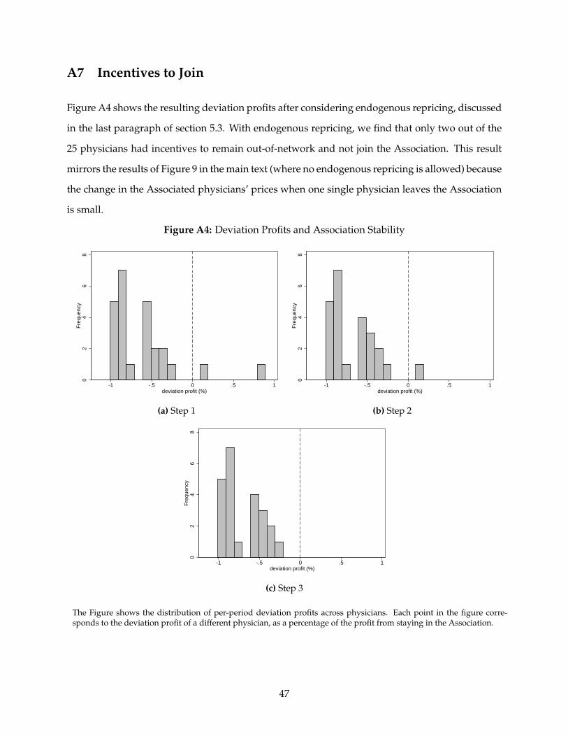
https://www.acog.org/~/media/Departments/Practice/ProfileofOb-gynPractice1991-2003.pdf

https://www.acog.org/~/media/Departments/Practice/ProfileofOb-gynPractice1991-2003.pdf

A7 Incentives to Join

Figure A4 shows the resulting deviation profits after considering endogenous repricing, discussed

in the last paragraph of section 5.3. With endogenous repricing, we find that only two out of the

25 physicians had incentives to remain out-of-network and not join the Association. This result

mirrors the results of Figure 9 in the main text (where no endogenous repricing is allowed) because

the change in the Associated physicians’ prices when one single physician leaves the Association

is small.

Figure A4: Deviation Profits and Association Stability

02

46

8F

requ

ency


(a) Step 1

02

46

8F

requ

ency


(b) Step 2

02

46

8F

requ

ency


(c) Step 3

The Figure shows the distribution of per-period deviation profits across physicians. Each point in the figure corre-sponds to the deviation profit of a different physician, as a percentage of the profit from staying in the Association.

47

trade associations and collusion among many agents

Documents