trade policies, household welfare and poverty alleviation ... · trade policies, household welfare...
TRANSCRIPT
TRADE POLICIES, HOUSEHOLD WELFARE AND POVERTY ALLEVIATION
CASE STUDIES FROM THE VIRTUAL INSTITUTE ACADEMIC NETWORK
U n i t e d n at i o n s C o n f e r e n C e o n t r a d e a n d d e v e l o p m e n tU n i t e d n at i o n s C o n f e r e n C e o n t r a d e a n d d e v e l o p m e n t
Intr
oduc
tion
Trade policies, household welfare and poverty alleviation:
Case studies from the Virtual Institute academic network
NEW YORK AND GENEVA, 2014

Note
The views expressed in this volume are those of the authors and do not necessarily reflect the views of the United Nations Secretariat.
The designations employed and the presentation of the material do not imply the expression of any opinion on the part of the United Nations concerning the legal status of any country, territory, city or area, or of its authorities, or concerning the delimitation of its frontiers or boundaries, or regarding its economic system or degree of development.
Exceptionally, references to currencies use the International Standard for currency codes (ISO 4217) of the International Organization for Standardization.
Material in this publication may be freely quoted or reprinted, but acknowledgement of the UNCTAD Virtual Institute is requested, together with a reference to the document number. A copy of the publication containing the quotation or reprint should be sent to the UNCTAD Virtual Institute, Division on Globalization and Development Strategies, Palais des Nations, 1211 Geneva 10, Switzerland.
The symbols of United Nations documents are composed of capital letters combined with figures. Mention of such a symbol indicates a reference to a United Nations document.
The UNCTAD Virtual Institute is a capacity-building and networking programme that aims to strengthen teaching and research of international trade and development issues at academic institutions in developing countries and countries with economies in transition, and to foster links between research and policymaking.
For further information about the UNCTAD Virtual Institute, please contact:
Ms. Vlasta MackuChief, Virtual InstituteDivision on Globalization and Development StrategiesUnited Nations Conference on Trade and DevelopmentE-mail: [email protected]://vi.unctad.org
UNCTAD/GDS/2014/3
© Copyright United Nations 2014All rights reserved

Intr
oduc
tion
The Philippines 29Distributional impact of the 2008 rice crisis in the PhilippinesGeorge Manzano and Shanti Aubren Prado
The former Yugoslav Republic of Macedonia 77Increasing the welfare effect of the agricultural subsidy programme for food crop production in the former Yugoslav Republic of MacedoniaMarjan Petreski
Argentina 119Welfare impact of wheat export restrictions in Argentina: Non-parametric analysis on urban householdsPaula Andrea Calvo
China 167 The consumption effect of the renminbi appreciation in rural ChinaDahai Fu and Shantong Li
Costa Rica 197Welfare effects of a change in the trade policy regime for rice in Costa RicaCarlos Eduardo Umaña-Alvarado
Peru 243Estimation of the pass-through and welfare effects of the tariff reduction for yellow corn in Peru between 2000 and 2011Carmen Cecilia Matta Jara and Ana María del Carmen Vera Ganoza
Nigeria 273The welfare impact in Nigeria of the Common External Tariff of the Economic Community of West African States: A distributional effects analysisOlayinka Idowu Kareem
Viet Nam 301Household welfare and pricing of rice: Does the Large-Scale Field Model matter for Viet Nam?Ngoc Quang Pham and Anh Hai La
Table of contents
Preface vContributors viii
Introduction 1Trade policies, household welfare and poverty alleviation – An overviewNina Pavcnik

iv

v
Intr
oduc
tion
Preface
In 2000, the world’s leaders set an ambitious agenda of Millennium Development Goals (MDGs) committing their nations to a new global part-nership to reduce extreme poverty, and setting out a series of time-bound targets for 2015. Many countries have been struggling to achieve these goals under circumstances that have deteriorated as a result of the global economic crisis. The target of halving extreme poverty between 1990 and 2015 is likely to be achieved thanks to the considerable fall in the poverty rate in Asian countries with large populations, such as China and India, but progress has been much slower in other regions, particularly in sub-Sa-haran Africa. Progress in achieving full and productive employment and decent work for all has been even less satisfactory as the recent deteriora-tion of the labour market has resulted in a decline in employment, push-ing more workers into vulnerable employment and poverty.
International trade can support the achievement of the MDGs in develop-ing countries and play a positive role in pro-poor growth and sustainable development. It can create employment, enhance access to technology and knowledge, raise productivity, increase the variety and quality of goods available to consumers, stimulate capital inflows, increase foreign ex-change earnings, and generate resources for sustainable development and poverty reduction. However, this positive relationship is not automatic and does not necessarily take place in all countries and contexts. Both national policies and international action need to be adopted and implemented to maximize the positive impact of trade on poverty. The design of effective national policies, as well as the formulation of negotiating positions for international fora dealing with trade issues, must be grounded in a thor-ough analysis of data, trends and experiences, and based on a careful as-sessment of the possible effects of various policy options and negotiation outcomes. In this respect, academic institutions and researchers are key to generating the analysis needed to inform policymaking.
To leverage researcher-policymaker cooperation that can help countries de-sign pro-poor trade policies, the UNCTAD Virtual Institute (Vi) launched a three-year (2012–2014) trade and poverty project aiming to strengthen the capacity of researchers in developing and transition countries. Advisory support to the project was provided by two experienced trade and poverty researchers, Alessandro Nicita from the UNCTAD Division on International Trade in Goods and Services and Commodities, and Amelia Santos-Paulino from the Division for Africa and Least Developed Countries. The objective of the project was twofold: first, to equip participating researchers with knowledge of the trade and poverty conundrum and the empirical tools needed to assess the impact of trade and trade-related policies on poverty

vi
Trade policies, household welfare and poverty alleviation
and income distribution; and second, to encourage these researchers to un-dertake policy-oriented studies on trade and poverty.
The first project objective was achieved by training researchers through an online course on trade and poverty analysis authored by Guido Porto (National University of La Plata, Argentina) and Nicolas Depetris Chauvin (African Center for Economic Transformation, Ghana, and University of Buenos Aires, Argentina), in collaboration with David Jaume (National University of La Plata). The course, developed by Vi webmaster Susana Olivares with assistance from Micaela Mumenthaler and Franziska Pfeifer, took place from 10 September to 30 November 2012. It was tutored by Nicolas Depetris Chauvin and Vi economist Cristian Ugarte, with techni-cal support from Susana Olivares, and graduated 77 researchers, including 29 women, from 45 developing and transition countries.
To further the second objective of the project – to encourage and facil-itate policy-oriented research – the online course analysed policy-rele-vant research papers, offered specific presentations and an online forum to discuss policy questions related to trade and poverty, and challenged par-ticipants to draft an essay proposing a research idea on a trade and pover-ty issue of relevance to national policymaking as part of the final course assignment. The top graduates of the course were invited to develop their essays into full proposals for research projects to be conducted in coop-eration with national policymakers. The 14 researchers whose proposals were selected for Vi support in March 2013 were paired with internation-al expert “mentors” who assisted them in the completion of their studies. These experts included UNCTAD’s Alessandro Nicita and Marco Fugazza (Division on International Trade in Goods and Services and Commodities), Amelia Santos-Paulino and Rashmi Banga (Division for Africa and Least Developed Countries), Piergiuseppe Fortunato (Division on Globalization and Development Strategies) and Claudia Trentini (Division on Investment and Enterprise). Other participating experts were Marion Jansen of the World Trade Organization’s Economic Research and Statistics Division, and online course co-author Nicolas Depetris Chauvin. The Vi team pro-vided comments and suggestions on the direction and content of the stud-ies and supported the authors during the drafting process.
The researchers benefited from a combination of online and face-to-face mentoring, the latter provided during a workshop in Geneva in June 2013. In addition to offering expert advice, the workshop included a session on writing policy briefs and communicating with policymakers in order to help researchers establish effective links with policymakers. The ex-perience of participating researchers confirmed that the interaction with

vii
Intr
oduc
tion
Preface
policymakers was useful in identifying important topics for policy anal-ysis, developing a better understanding of the researched sectors and related government policies, gaining access to relevant data, and under-standing the constraints policymakers may face in implementing the re-searchers’ recommendations.
This book is a collection of country case studies emanating from the Virtual Institute’s trade and poverty project. The studies were drafted by researchers from universities, think tanks, and government ministries in Argentina, China, Costa Rica, the former Yugoslav Republic of Macedonia, Nigeria, Peru, the Philippines, and Viet Nam. The studies were peer-re-viewed by Nina Pavcnik from Dartmouth College, Petia Topalova from the John F. Kennedy School of Public Policy at Harvard University, Isidro Soloaga from the Universidad Iberoamericana Ciudad de México, and Marcelo Olarreaga from the University of Geneva. Vi economist David Zavaleta contributed to the final stages of the preparation of the book. Nina Pavcnik served as the editor and offered additional technical comments on all the studies. The book was copy-edited by David Einhorn and Martha Bonilla; Eveliina Kauppinen and Mireille Velazquez assisted in formatting the text. Design and layout were created by Hadrien Gliozzo, with photos contributed by Irene Becker, Leniners, Lars Lundqvist, Jasna Susha and Julien Yamba, and advice on the cover by Andrés Carnevali. The publica-tion process was managed by Nora Circosta.
I would in particular like to extend special thanks to Cristian Ugarte, who managed the entire project and was the driving force behind its success-ful completion.
Finally, our gratitude goes to the United Nations Department of Economic and Social Affairs and the Government of Finland, whose trust and finan-cial contributions allowed us to make this project a reality, and to all the national policymakers who supported our researchers.
Vlasta MackuChiefUNCTAD Virtual Institute

viii
Trade policies, household welfare and poverty alleviation
Contributors
Editor
Nina PavcnikDartmouth College, Bureau for Research and Economic Analysis of Development (BREAD), and National Bureau of Economic Research (NBER), United States of America; Centre for Economic Policy Research (CEPR), United Kingdom of Great Britain and Northern [email protected]
Authors
Paula Andrea CalvoUniversidad de San Andrés, [email protected]
Dahai Fu Central University of Finance and Economics, [email protected]
Olayinka Idowu Kareem European University Institute, [email protected]
Anh Hai LaViet Nam Academy of Social Sciences, Viet [email protected]
Shantong LiDevelopment Research Center of the State Council, [email protected]
George Manzano University of Asia and the Pacific, the [email protected], [email protected]

ix
Intr
oduc
tion
Carmen Cecilia Matta JaraMinistry of Foreign Trade and Tourism, [email protected], [email protected]
Marjan Petreski University American College Skopje, the former Yugoslav Republic of [email protected]
Ngoc Quang PhamInternational Labour Organization Country Office for Viet Nam, Viet [email protected]
Shanti Aubren PradoUniversity of Asia and the Pacific, the Philippines [email protected]
Carlos Eduardo Umaña-Alvarado Academia de Centroamérica, Costa Rica [email protected]
Ana María del Carmen Vera Ganoza Ministry of Foreign Trade and Tourism, [email protected], [email protected]

x
Trade policies, household welfare and poverty alleviation
Introduction

1
Intr
oduc
tionTrade policies, household welfare and
poverty alleviation – An overview
* The author would like to thank Carla Larin from Dartmouth College for her excellent research assistance.
Nina Pavcnik*
1 Introduction
During the past three decades, low- and middle-income countries have become increasingly integrated into the global economy. Exports of low-income countries grew from 26 to 55 per cent of their gross domes-tic product (GDP) between 1994 and 2008 (Hanson, 2012). Exports of mid-dle-income countries increased from 25 to 55 per cent of their GDP during the same period. Hanson (2012) attributes the heightened global engage-ment to declines in trade costs through large-scale trade liberalizations in developing countries and the removal of barriers to low-skilled goods such as apparel and textiles in developed country markets. Greater in-ternational fragmentation of production and increased demand for com-modities, fueled by growth in India and China, have also contributed to this trend.
This globalization of less-developed countries has sparked a debate in ac-ademic and policy circles about the relationship between international trade and poverty. Global poverty has declined: the share of people living on less than a dollar per day dropped from 52 per cent in 1981 to 22 per cent in 2008 (Chen and Ravallion, 2012). But to what extent is this decline related to growth in international trade? How do the poor fare as low-in-come countries embrace more liberalized trade policies and expose do-mestic markets to increased import competition? Do the poor benefit as low-income countries gain access to high-income export markets? Several recent surveys and studies address these questions and discuss the chan-nels through which international trade might affect poverty (Goldberg and Pavcnik, 2004; Winters et al., 2004; Harrison, 2007; Pavcnik, 2008).
2
Trade policies, household welfare and poverty alleviation
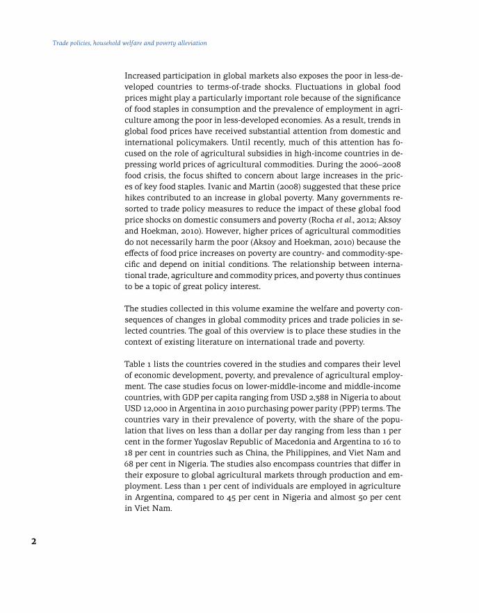
Increased participation in global markets also exposes the poor in less-de-veloped countries to terms-of-trade shocks. Fluctuations in global food prices might play a particularly important role because of the significance of food staples in consumption and the prevalence of employment in agri-culture among the poor in less-developed economies. As a result, trends in global food prices have received substantial attention from domestic and international policymakers. Until recently, much of this attention has fo-cused on the role of agricultural subsidies in high-income countries in de-pressing world prices of agricultural commodities. During the 2006–2008 food crisis, the focus shifted to concern about large increases in the pric-es of key food staples. Ivanic and Martin (2008) suggested that these price hikes contributed to an increase in global poverty. Many governments re-sorted to trade policy measures to reduce the impact of these global food price shocks on domestic consumers and poverty (Rocha et al., 2012; Aksoy and Hoekman, 2010). However, higher prices of agricultural commodities do not necessarily harm the poor (Aksoy and Hoekman, 2010) because the effects of food price increases on poverty are country- and commodity-spe-cific and depend on initial conditions. The relationship between interna-tional trade, agriculture and commodity prices, and poverty thus continues to be a topic of great policy interest.
The studies collected in this volume examine the welfare and poverty con-sequences of changes in global commodity prices and trade policies in se-lected countries. The goal of this overview is to place these studies in the context of existing literature on international trade and poverty.
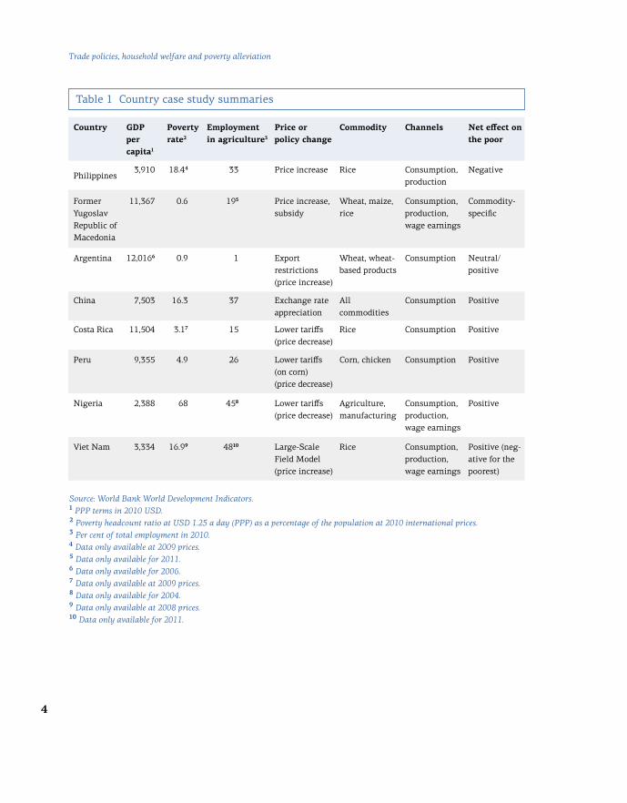
Table 1 lists the countries covered in the studies and compares their level of economic development, poverty, and prevalence of agricultural employ-ment. The case studies focus on lower-middle-income and middle-income countries, with GDP per capita ranging from USD 2,388 in Nigeria to about USD 12,000 in Argentina in 2010 purchasing power parity (PPP) terms. The countries vary in their prevalence of poverty, with the share of the popu-lation that lives on less than a dollar per day ranging from less than 1 per cent in the former Yugoslav Republic of Macedonia and Argentina to 16 to 18 per cent in countries such as China, the Philippines, and Viet Nam and 68 per cent in Nigeria. The studies also encompass countries that differ in their exposure to global agricultural markets through production and em-ployment. Less than 1 per cent of individuals are employed in agriculture in Argentina, compared to 45 per cent in Nigeria and almost 50 per cent in Viet Nam.

3
Trade policies, household welfare and poverty alleviation – An overview
Intr
oduc
tion
The studies address the relationship between globalization and poverty in the context of two broad themes. One set of studies examines the welfare consequences of the recent increases in global food prices. The other set of studies examines the welfare effects of trade policy and exchange rate changes. Table 1 lists the price change and/or specific policies and com-modities that are the focus of each country’s case study.
The research uses a common methodology based on household-level sur-veys, originally developed by Deaton (1989), to examine the welfare con-sequences of international trade. The focus is on the short-term effect of price changes through household consumption, production and wage earnings, which in turn affect household welfare and poverty. While the studies could in principle examine the role of all three components, data constraints at times confine the analysis to a subset of the channels. The channels considered in each country are also specified in Table 1.
The studies yield insights about the relationship between trade policy, changes in commodity prices, and poverty. Most importantly, they provide additional support for the conclusion by Aksoy and Hoekman (2010) that it is not possible to generalize about how higher food prices affect the poor. The consequences of commodity price changes for poverty through the channels examined in this volume are country-specific. Net effects on the poor for each country case study are summarized in Table 1. They depend on the impact of the trade policy change on domestic prices, the exposure of the poor households to price fluctuations as producers and consumers of the good, the exposure of these households to price shocks through wage earnings, and the magnitude of the price changes.
For example, while the rural poor tend to be harmed by increases in the price of rice in the Philippines, they benefit from an increased price of maize in the former Yugoslav Republic of Macedonia. This difference stems from the fact that the rural poor in the Philippines tend to be net consumers of rice, while the rural poor in the former Yugoslav Republic of Macedonia are net producers of the commodity that experienced a large price increase. The case of the former Yugoslav Republic of Macedonia fur-ther illustrates that the effects on poverty might depend on the commodi-ty under consideration.
4
Trade policies, household welfare and poverty alleviation
Source: World Bank World Development Indicators.1 PPP terms in 2010 USD. 2 Poverty headcount ratio at USD 1.25 a day (PPP) as a percentage of the population at 2010 international prices. 3 Per cent of total employment in 2010.4 Data only available at 2009 prices.5 Data only available for 2011.6 Data only available for 2006.7 Data only available at 2009 prices.8 Data only available for 2004. 9 Data only available at 2008 prices.10 Data only available for 2011.
Country GDP per capita1
Poverty rate2
Employment in agriculture3
Price or policy change
Commodity Channels Net effect on the poor
Philippines3,910 18.44 33 Price increase Rice Consumption,
productionNegative
Former Yugoslav Republic of Macedonia
11,367 0.6 195 Price increase, subsidy
Wheat, maize, rice
Consumption, production, wage earnings
Commodity- specific
Argentina 12,0166 0.9 1 Export restrictions(price increase)
Wheat, wheat-based products
Consumption Neutral/positive
China 7,503 16.3 37 Exchange rate appreciation
All commodities
Consumption Positive
Costa Rica 11,504 3.17 15 Lower tariffs(price decrease)
Rice Consumption Positive
Peru 9,355 4.9 26 Lower tariffs (on corn) (price decrease)
Corn, chicken Consumption Positive
Nigeria 2,388 68 458 Lower tariffs(price decrease)
Agriculture, manufacturing
Consumption, production, wage earnings
Positive
Viet Nam 3,334 16.99 4810 Large-Scale Field Model (price increase)
Rice Consumption, production, wage earnings
Positive (neg-ative for the poorest)
Table 1 Country case study summaries

5
Trade policies, household welfare and poverty alleviation – An overview
Intr
oduc
tion
The studies also provide institutional details about the organization of the supply chain through which commodities are delivered from producers to consumers. Several studies highlight that it is crucial to consider how price changes are passed through in this supply chain. For example, stud-ies on Viet Nam and Argentina suggest that the main beneficiaries of high-er prices might be the middlemen and intermediaries. Likewise, studies on Costa Rica and Peru suggest that the welfare gains of consumers from reductions in import tariffs on a good might be reduced when wholesale importers do not fully pass on cost savings to consumers of final goods. Further exploration of the organization of the supply chain can therefore be a fruitful topic for future research.
Section 2 of this overview reviews the channels through which interna-tional trade might affect poverty and discusses the empirical evidence on the importance of these channels in practice. Section 3 discusses the mech-anisms through which international trade affects poverty in the studies compiled in this volume and overviews the common methodology. Section 4 summarizes the findings of the studies that focus on the welfare conse-quences of recent increases in global food prices. Section 5 reviews the studies that examine the welfare effects of trade policy and exchange rate changes. Section 6 puts forth conclusions.
2 International trade and poverty – An overview
This section reviews the channels through which international trade might affect poverty and discusses the empirical evidence on the importance of these channels in practice.
2.1 International trade and poverty: Economic growth
Economists agree that economic growth is potentially the most important channel to reduce poverty and that international trade might play an im-portant role in this process. This argument requires one to first examine the relationship between international trade and economic growth, and then consider how trade-induced economic growth might affect poverty.
Theoretically, the relationship between international trade and growth is ambiguous, especially for lower-income countries that might not have comparative advantage in sectors that generate dynamic gains from trade (Rodriguez and Rodrik, 2001). International trade raises average incomes through static gains from trade due to specialization according to compar-ative advantage and economies of scale, among other factors. However, if

6
Trade policies, household welfare and poverty alleviation
specialization according to comparative advantage contracts sectors that are engines of growth, it could outweigh the benefits of static gains from trade and reduce growth in less-developed countries. Several empirical studies (most notably Frankel and Romer, 1999) find that countries that trade more tend to have higher incomes, but a robust relationship be-tween international trade and growth across countries has been elusive (see Rodriguez and Rodrik, 2001, for a critique). That being said, it is diffi-cult to point to countries that were able to grow over long periods of time without opening up to trade (Irwin, 2004). So the lack of robust evidence certainly does not imply that international isolation leads to growth. One major challenge in this literature is determining the causality of wheth-er countries that trade more (or observe an increase in international trade) subsequently experience higher growth, or whether high-growth coun-tries simply engage more in international trade.
Several recent studies have made advances in addressing the causality prob-lem and confirm a positive link between international trade and growth. For example, Feyrer (2009) found that declines in trade associated with the clo-sure of the Suez Canal were associated with reductions in income in coun-tries that rely heavily on the canal for transportation. Estevadeordal and Taylor (2013) compared changes in growth rates in less-developed countries that participated in the Uruguay Round of the World Trade Organization (WTO) negotiations with changes in growth rates among non-participants. They found that declines in import tariffs increased GDP growth among the countries that liberalized their trade. Increased growth rates stemmed mainly from declines in tariffs on capital goods and imported intermediate inputs rather than reductions in tariffs on consumer goods. This highlights the importance of gains from trade that operate through increased efficien-cy and innovation in the production process. The importance of import-ed inputs and technology for efficiency and innovation in less-developed countries is corroborated by microeconomic firm-level evidence (Amiti and Koenings, 2007; Topalova and Khandelwal, 2011; Goldberg et al., 2010). While this more recent evidence suggests a robust and more nuanced posi-tive relationship between international trade and economic growth, the ac-ademic debate on the topic continues.
In order to consider how international trade affects poverty via growth, one needs to examine how trade-induced economic growth affects poverty
– a link which is very difficult to establish. Widely cited works by Dollar and Kraay (2002, 2004) suggest that trade – via growth – is good for the poor by showing that countries with increased participation in international trade experience greater declines in poverty. However, these findings have been heavily debated (Ravallion, 2001; Deaton, 2005). Trade-induced economic

7
Trade policies, household welfare and poverty alleviation – An overview
Intr
oduc
tion
growth could help the poor (for example, by increasing their earning op-portunities through the creation of employment for less-educated individ-uals), but it could also circumvent the poor (Ravallion, 2001).
2.2 International trade and poverty: Relative prices, wages, and employment
Most studies that examine the relationship between international trade and poverty look at the direct effect on poverty that might operate through changes in relative prices, wages and employment. A survey by Goldberg and Pavcnik (2004) discussed trade-related mechanisms that could affect poverty through earnings of less-educated workers, industry wage pre-miums, occupational wage premiums, and effects on worker employment and/or unemployment. They suggested that the effects of internation-al trade on poverty are country-specific. The effects depend on the expo-sure of the poor to international trade through employment opportunities and the above-mentioned sources of income, the impact of trade on these sources of income, and the nature of the trade policy change in the coun-try in question.
Several recent studies have directly examined the effect of trade liberali-zation on poverty.1 Goldberg and Pavcnik (2007) found no relationship be-tween international trade and poverty in urban Colombia. Poverty among urban households in Colombia was relatively low, with less than 3 per cent of households living below the dollar-a-day poverty line during the time frame under study. The urban poor tended to live in households with an unemployed household head, so the main mechanism through which in-ternational trade could affect poverty was through its effects on unemploy-ment. The study did not find any evidence that declines in import tariffs in Colombia were associated with increased unemployment. As a result, it is not surprising that the study also did not find any evidence that import tariff declines affected urban poverty.
Several studies have found a statistically significant impact of internation-al trade on poverty in countries with relatively high poverty rates at the onset of trade policy reforms. In these cases, the effects of trade reform on poverty depend in part on the nature of trade liberalization and the ease of worker mobility. For example, India experienced large declines in poverty during the 1990s. Topalova (2007, 2010) found that poverty declined less in Indian districts that were more exposed to import tariff declines, especially
1 Several of these studies were published in Harrison (2007), a volume on globalization and poverty.

8
Trade policies, household welfare and poverty alleviation
in areas located in states with stringent labour laws. Indian workers in in-dustries with larger tariff cuts experienced declines in relative wages, so the study conjectured that limited mobility of individuals living in these districts precluded them from moving to the areas with new employment opportunities. Kovak (2011) also documented declines in regional wag-es and evidence of limited regional labour mobility in the aftermath of trade liberalization in Brazil. As in the case of India, the Brazilian reform consisted of lowered import barriers to trade. McCaig (2011), on the other hand, found that poverty dropped more in Vietnamese provinces that were better positioned to benefit from increased export opportunities after Viet Nam signed the bilateral trade agreement with the United States. Workers in provinces that were more exposed to export opportunities, especially workers with less education, experienced increases in wages in response to declines in tariffs on Vietnamese exports in the United States, which translated into lower poverty.
Overall, these studies highlight that the effects of international trade on poverty depend on the nature of the trade reform, the effects of interna-tional trade on sources of income/employment, and the importance of these channels for the households at the bottom of the income distribu-tion in the country in question.
2.3 International trade and poverty: Relative prices, and net consumption and production
The studies reviewed in Section 2.2 examine the link between internation-al trade and poverty that operates through the response of wages and em-ployment opportunities of individuals to trade-induced changes in relative prices of goods. Trade-induced changes in relative prices of goods might also affect poverty through exposure of households as consumers and pro-ducers of goods (see surveys by Goldberg and Pavcnik, 2004, and Harrison, 2007). Most individuals in low-income countries do not work for wages and are instead self-employed in a household business or farm. However, these households might be exposed to trade-induced price fluctuations as producers of commodities experiencing price changes. Likewise, house-holds in low-income countries are affected by price fluctuations as con-sumers. Fluctuations in the prices of food staples might be particularly important because poor households in these economies often spend 60 to 80 per cent of their household budget on staples.
The literature that examines the above-mentioned effects of trade policy on poverty through net consumption and production builds on the meth-odology of Deaton (1989) and focuses on the first-order effects of price

9
Trade policies, household welfare and poverty alleviation – An overview
Intr
oduc
tion
changes on the welfare of households, holding the consumption and pro-duction bundles of households fixed.
Overall, the literature concludes that the effects of trade liberalization on poverty operating through these channels are case-specific. They depend on the nature of the trade policy change, exposure of the poor to trade-in-duced price fluctuations as consumers, producers and wage earners, sensi-tivity of wages to price changes, and the magnitude of the price changes.
Potentially the most influential among these studies are Porto (2006) and Nicita (2009). Porto (2006) examined the effect of the Common Market of the South (MERCOSUR) on urban Argentine households through con-sumption and earnings channels. The study found that import tariff re-ductions induced by MERCOSUR benefited poor households in Argentina. Tariffs declined relatively more on skilled-labour-intensive goods than un-skilled-labour-intensive goods, leading to increased relative prices of un-skilled-labour-intensive goods. As predicted by the Hecksher-Ohlin model, this translated into increased wages of unskilled workers and declines in earnings of skilled workers. Because most workers from poor households in urban Argentina tend to be less educated, the earnings in poor house-holds increased. At the same time, poor households experienced a decline in welfare through the consumption channel because they tend to consume relatively more of the goods whose price increased (such as unskilled-la-bour-intensive goods). However, the welfare gains through earnings ex-ceeded the welfare losses through consumption, leading to overall welfare gains for the poor.
Nicita (2009) studied the effect of Mexico’s trade liberalizations during the 1980s and 1990s on Mexican households through consumption, pro-duction and wage earnings channels. Import tariff reductions lowered the prices of agricultural and manufacturing goods, and these lower prices benefited households through the consumption channel at all income lev-els. However, welfare gains were smaller for the poor because they relied more heavily on self-produced consumption. Lower prices of agricul-tural goods negatively affected poor households through the production channel, and the poor were also not well positioned to gain through the wage earnings channel. The trade reform was associated with a slight in-crease in the wages of educated workers that mainly benefited higher-in-come households composed of individuals with many years of completed schooling. Overall, the study found that the welfare gains through con-sumption outweighed the welfare losses through production for the poor. It also concluded that the trade reform was more beneficial for households living closer to the United States border and in urban areas.
10
Trade policies, household welfare and poverty alleviation
The above studies focus on first-order effects of price changes on the wel-fare of households, holding the consumption and production bundles of households fixed. Households might respond to price changes by altering consumption and production. A related study that examines the importance of international trade for the welfare of poor households is Brambilla et al. (2012), who examined the effect of anti-dumping duties on catfish imposed by the United States on Vietnamese households. The study found that high-er import tariffs lower production and investment, and reduce the income of Vietnamese households that rely on catfish as their source of livelihood. The study illustrates that the usual methodology that focuses on first-order short-term effects of price changes through consumption and production might potentially ignore welfare consequences associated with longer-term responses to price shocks that operate through changes in household consumption, production and investment decisions (Porto, 2010).
3 Overview of studies in this volume
The studies in this volume focus on the relationship between internation-al trade and poverty that operates through channels discussed in Section 2.3. While the studies cover a variety of topics, they all examine short-term first-order effects of price changes on household welfare that operate through household consumption and production.
The welfare analysis uses a common methodology that is based on cross-sec-tional household-level data that contain information about household in-come (and its sources) and household expenditures allocated to different consumption items. The data are representative of households along the entire distribution of income, allowing for direct examination of the wel-fare consequences of price fluctuations for poor households. As in Deaton (1989), household budget shares of a commodity measure a household’s exposure to price changes through the consumption channel. Likewise, the household income share stemming from production of a commodity measures a household’s exposure to price changes through the production channel. A household’s exposure to price changes through labour earnings
– the wage channel – depends on the share of these earnings in household income and the elasticity of wages with respect to a price change.
The studies use either information on actual price changes or a price change predicted by a policy adjustment, such as a change in an import tariff or exchange rate appreciation. The framework can be used to simu-late the effect of price changes on household welfare, taking into account differences in households’ exposure to price changes through these three

11
Trade policies, household welfare and poverty alleviation – An overview
Intr
oduc
tion
2 The description of each study in Sections 4 and 5 draws on facts and policy descriptions from the respective studies, unless otherwise noted. Please refer to the individual studies for original references.
channels. While all studies could in principle examine the role of all chan-nels, data constraints at times confine the analysis to the first-order wel-fare effects of price changes operating through consumption.
The studies apply this framework to address two broad topics. One set of studies examines the welfare consequences of the increases in global com-modity prices during the 2008–2010 food crisis. These studies focus on the Philippines, the former Yugoslav Republic of Macedonia and Argentina. Section 4 summarizes their findings. The other set of studies – on China, Costa Rica, Peru, Nigeria and Viet Nam – examines the welfare effects of trade policy and exchange rate policy, and is reviewed in Section 5.2
4 The effects of global food price increases
Several studies explore the short-term welfare implications for the poor of price increases during the 2006–2008 food crisis. This discussion is relat-ed to the discourse on the consequences of agricultural subsidies in rich countries for the terms of trade of low-income countries. These subsidies lower world prices of commodities, generating terms-of-trade losses for countries that are net exporters of these commodities, while benefiting countries that are net importers of the goods.
Research suggests that the poorest countries are often net importers of commodities which are subject to agricultural subsidies (Panagariya, 2006; Valdes and McCalla, 1999; McMillan et al., 2007). They might there-fore be adversely affected by the elimination of these subsidies. The main beneficiaries of the elimination of agricultural subsidies are expected to be large net exporters of agricultural goods such as Brazil (Panagariya, 2006; Valdes and McCalla, 1999), that is, lower-middle-income and middle-in-come countries. This literature highlights that the overall effect of recent price hikes on countries depends on whether a country is a net producer or a net consumer of the good. In aggregate, the surges in prices benefit countries that are net exporters of the food staple experiencing the price increase, while harming countries that are net importers of the good.
It is important to emphasize that in a country that might largely benefit from a price increase, poverty can increase or decrease. Within countries, price hikes generate winners and losers. A price increase of a good raises

12
Trade policies, household welfare and poverty alleviation
the welfare of households that are net producers of the good, and reduces the welfare of households that are net consumers of the good. The conse-quences of price hikes for poverty depend crucially on whether the house-holds at the bottom of the income distribution are net consumers or net producers of the good (Aksoy and Hoekman, 2010).
4.1 Effects on importing countries
The above discussion suggests that recent increases in global food prices might reduce aggregate welfare in countries that are net consumers of the good that experiences a price increase. This does not imply, however, that the poor in import-competing countries are necessarily worse off. The con-sequences of the price increases for the welfare of the poor in import-com-peting countries are country- and commodity-specific. The studies on the Philippines and the former Yugoslav Republic of Macedonia included in this volume highlight these nuances and illustrate the importance of us-ing micro-survey data to better understand the relationship between glob-al increases in food prices and poverty.
The Philippines: Rice
The study on the Philippines examines the impact of the 2008 rice crisis on household welfare in the country. During the crisis, world rice prices more than doubled. As one of the largest importers of rice in the world, the Philippines suffered a terms-of-trade loss and a potentially sizable ag-gregate welfare decline.
The study examines the effects of price increases on poverty through household consumption and production. Because a typical Filipino house-hold is a net consumer of rice, the study finds that more households are negatively affected by the increase in rice prices. Rice accounts for about 13 per cent of household spending (a third of spending on food) in a typical Filipino household. Consistent with Engel’s Law, the poorest households in the Philippines spend between 20 to 25 per cent of their budget on rice, with the share declining to less than 5 per cent among the relatively richer households. Consequently, the uptick in domestic rice prices had a particu-larly large negative effect on the welfare of the poorest households be-cause they were the most exposed to rice price hikes through consumption.
The price shock lowered the welfare of poor households in rural and ur-ban areas, but the price increase is predicted to have had a more detri-mental effect on the urban poor. The finding of negative welfare effects on the rural poor might be surprising at first because rice cultivation is
13
Trade policies, household welfare and poverty alleviation – An overview
Intr
oduc
tion
concentrated in rural areas, with 22 per cent of the rural population grow-ing rice. However, rice cultivation is not an important income source for the poorest rural households.
The study also considers gender differences by comparing the income and expenditure patterns of female- and male-headed households. While the patterns of expenditure are similar for both types of households, dif-ferences are found in the composition of income: rice production is rel-atively more important in male-headed households, probably because female-headed households derive income from other non-rice produc-tion-related activities. As a result, female-headed households are more vul-nerable to price hikes.
Overall, the study illustrates that households adversely affected by the rice crisis outnumber households that were better off, with the poor bearing disproportionate welfare losses. The main beneficiaries of the rice price increases were richer agricultural households, which tend to be net pro-ducers of rice.
The study highlights the effects of rice price increases on household wel-fare through the household level of rice consumption and production, but not through household wage earnings. This channel might play the larg-est role in regions where rice cultivation is concentrated if rice price in-creases are large enough to increase local demand for agricultural labour and thus local wages.
The former Yugoslav Republic of Macedonia: Wheat, maize and rice
Similar to the Philippines, the former Yugoslav Republic of Macedonia experienced a negative terms-of-trade shock during the recent food crisis. The country is a net importer of wheat, maize and rice, the three crops that experienced a large price increase between 2006 and 2012. However, GDP per capita in the country is substantially higher than in the Philippines, so a typical Macedonian household is substantially less exposed to these price shocks through consumption and production than a typical house-hold in the Philippines.
Rice consumption and production play a small role in the lives of aver-age Macedonian households, accounting for less than 1 per cent of house-hold expenditure and less than half a per cent of income. Even among rural households, expenditure on rice accounts for less than 1 per cent of the household budget and about 1 per cent of household income.

14
Trade policies, household welfare and poverty alleviation
An average Macedonian household is more exposed to fluctuations in pric-es of wheat and maize, spending about 2 per cent of household expenditure on wheat and maize and receiving 5 per cent of income from the two com-modities. Wheat and maize play a substantially larger role in the lives of rural households, contributing to about 20 per cent of household income and 4 per cent of household expenditure. The two commodities account for a small share of average urban household expenditure (0.8 per cent) and income (0 per cent).
The study highlights differences in the short-term effects of increased global prices on households through consumption, production, and wage earnings. Price increases of all three commodities reduced the welfare of urban households that are net consumers of these commodities. The poorest urban households, especially female-headed ones, experienced the largest decline in welfare.
Price increases in wheat and maize were beneficial for rural households along the entire income distribution, with the poorest households bene-fiting the most from price hikes. However, conditional on per capita ex-penditure, male-headed households benefited substantially more than female-headed ones. The cultivation of wheat and maize occurs mainly in male-headed households, and this accounts for the observed differences in welfare changes by gender. The poorest female-headed rural households do not engage significantly in cultivation and are most negatively affect-ed by price increases.
Rice accounts for a substantially smaller share of the household budget, so the effects of rice price increases were small in magnitude. Rice price in-creases benefited mainly male-headed rural households in the middle and upper level of income distribution, as these households are more likely to cultivate rice. Poor, female-headed rural households were particularly ad-versely affected.
The study also evaluates the effectiveness of a production subsidy imple-mented by the government of the former Yugoslav Republic of Macedonia in 2006 to encourage production of wheat and maize and improve the livelihoods of the rural poor. The results suggest that the subsidy did not reverse the trend of declining domestic production of cereals. Neither was it an effective tool for combating poverty, in part because poor ru-ral female-headed households and poor urban households tend to be net consumers rather than producers of the subsidized crops. The study pro-poses an alternative scheme for subsidy disbursement that better tar-gets the poorest sub-groups and aims to encourage production among

15
Trade policies, household welfare and poverty alleviation – An overview
Intr
oduc
tion
female-headed households and poor urban households. While the alterna-tive subsidy scheme might better target the poor than the original one, a policy tool that more directly addresses poverty alleviation, such as direct cash transfers to the poor or other forms of a social safety net aimed at the poor, might be even more effective. Overall, the study is a clear illustra-tion of the usefulness of micro-level surveys in assessing the short-term first-order effect of price changes induced by government policy.
4.2 Export restrictions in response to the food crisis
The 2006–2008 food crisis deteriorated the terms of trade of importers such as the Philippines and the former Yugoslav Republic of Macedonia, while improving the terms of trade of exporting countries. Exporting countries experience a net benefit from the price hikes. However, the price shocks can also increase poverty in these countries by disproportionate-ly harming the households at the bottom of the income distribution if these households are net consumers of the good. Faced with these con-cerns, many exporting countries responded to the food crisis by restrict-ing exports of key food staples through the imposition of export quotas and by raising export taxes. Rocha et al. (2012) reported 85 new export re-strictions between 2008 and 2010, the majority of them imposed on wheat, maize and rice, which are all staples that account for a large share of the household budget in low- and middle-income countries.
In theory, export restrictions such as export taxes and quotas lower domes-tic prices of staples. Faced with an increased cost of exporting, domestic firms divert export sales to domestic markets, hereby increasing the sup-ply and consequently lowering internal prices. This benefits domestic con-sumers (who can now consume more of the good and at lower prices) at the expense of domestic producers (who now produce less and sell at low-er prices).
Export restrictions do not constitute first-best economic policies for pover-ty reduction during times of price hikes. In addition, these measures only alleviate the increases in poverty during times of price hikes if the poor are actually net consumers of the good in question. This is more likely to hold for urban households, but it is less clear for rural households.
Argentina: Export restrictions, subsidies and international wheat prices
The study on Argentina contributes to the understanding of these issues by focusing on the potential effects of quantitative restrictions imposed

16
Trade policies, household welfare and poverty alleviation
on wheat exports in 2006 on the welfare of urban households in Argentina. Argentina is a net exporter of wheat, with exports accounting for over 60 per cent of production and over 7 per cent of the country’s total ex-ports during the period under study. Argentina introduced export duties on wheat in 2002, followed by quantitative export restrictions on wheat in 2006. Domestic price ceilings and subsidies for millers and wheat produc-ers were also put in place in 2007.
As a result, millers were to purchase wheat from producers at a low “in-ternal supply price”. The government then paid the mills a subsidy in case they bought wheat domestically at a higher price than the internal supply price, and provided producers a subsidy compensating them in case the price in the international market, adjusted by export duties, exceeded that in the domestic market. These policies were implemented to curb domes-tic inflation in cereals and wheat-based products (such as bread and pasta) during the period of high global prices and to ensure sufficient domestic provision of wheat.
Export restrictions benefited Argentine consumers of wheat, including producers and consumers of wheat-based products, at the expense of Argentine wheat producers. While the subsidies might have in part com-pensated Argentine wheat producers, they required government funding. How effective were these policies in curbing inflation and protecting the poor from high food prices?
The author examines the consequences of these policies for the welfare of Argentine urban households through household consumption of wheat-based products. A typical Argentine household spends about 6 per cent of its budget on wheat-based products such as bread and pasta, but export re-strictions were associated with negligible welfare gains for urban consum-ers. Wheat-based products account for a substantially higher budget share among poor households (about 11 per cent) than among households in the top 5th quintile of the income distribution (about 3 per cent). Although declines in prices of wheat-based goods benefited the poorest households the most, the magnitude of these effects also turns out to be quite limited.
Negligible welfare effects are attributed to the minimal influence that high international wheat prices have on prices of wheat-based products. Wheat accounts for about 10 per cent of the cost of producing wheat-based prod-ucts, with inputs such as labour, utilities and rent playing a substantial-ly more important role. According to the study, the price of wheat-based products would only increase 1 per cent more in the absence of export quotas.

17
Trade policies, household welfare and poverty alleviation – An overview
Intr
oduc
tion
The study also examines the interaction of export restrictions with domes-tic policy measures. When combined with ceiling prices and subsidies to the milling industry, welfare effects on households are larger, although they continue to be small in magnitude. These results are indicative of the failure of the policies to achieve welfare goals, and might help direct the design and implementation of future policies.
The study highlights the importance of examining the organization of the entire supply chain. The author argues that the likely main beneficiar-ies of the policy were millers and exporters because they usually hold ex-port licences. The establishments that received export licences were able to purchase wheat at low prices controlled by price ceilings, and then ex-port it at high international prices. The author suggests that export restric-tions actually reduced competition among the millers and exporters, thus strengthening their monopoly position over wheat producers and further reducing the price of wheat received by the farmers.
The effectiveness of export restrictions in insulating domestic consum-ers from price increases and reducing poverty could diminish further once global externalities of a trade policy change are taken into account. When several large exporters simultaneously impose export restrictions, this limits the world supply and leads to the escalation of international pric-es. Recent research by Anderson et al. (2013) pointed out that, once the ef-fects of export restrictions on world prices are considered, the declines in global poverty attributed to these restrictions are substantially reduced.
5 Effects of appreciation and trade policy
Governments can also influence the domestic prices of goods through ex-change rate policy and trade policy. A set of studies in this volume exam-ines the short-term consequences of such policies on household welfare.
China: Effects of exchange rate appreciation
In July 2005, China ceased to fix its exchange rate against the United States dollar and began to appreciate the renminbi, which led to a 30 per cent ap-preciation of the Chinese currency against the dollar.
The study on China examines the impact of the appreciation on changes in welfare of Chinese households through consumption. It first determines the effect of the renminbi appreciation on domestic prices, and then anal-yses the subsequent effect of these price changes on household welfare

18
Trade policies, household welfare and poverty alleviation
through consumption. The analysis focuses on rural China, where most poor households are located. According to the study, in 2007, 14 per cent of rural households and less than half a per cent of urban households in China lived on less than a dollar per day.
Appreciation in the nominal exchange rate of renminbi could exert down-ward pressure on prices of domestic substitute products in China by low-ering prices of competing imported goods and by reducing the demand for Chinese export goods abroad. The estimates confirm that the appre-ciation lowered consumer prices of goods in China, with the exception of medical care and durable goods. The authors attribute the lack of decline in prices in these two areas to imperfect substitutability of domestic and foreign medicines (most Chinese consumers tend to consume domestical-ly produced medicines) and to the fierce competition within China among domestic producers of durable goods, which translates into the prices of these products rarely being affected by the currency appreciation. Food products and housing experienced the largest drop in prices, in part due to reduced prices of fuel. Because purchased food products account for the largest share of the household budget (on average between 19 to 33 per cent in various regions), the appreciation generated significant wel-fare gains for all households by reducing their consumption expenditure.
However, poor households benefited less from appreciation than richer households. The lower benefits of the poor in rural areas stem from a heavy reliance on self-produced consumption (which is not affected by apprecia-tion) and a subsequently lower share of purchased food. Among the items affected by appreciation, poorer households consume less of the goods that experienced greater price declines. The authors also show that apprecia-tion generated larger gains for households living in provinces with more developed market institutions, because appreciation pass-through to do-mestic prices is higher (and thus prices lower) in these regions. Inland provinces in Western China tend to have less developed markets, so the poor households in these provinces benefited the least from appreciation. Conditional on income, households in coastal areas are better positioned to gain than households in inland provinces.
The study focuses on the impact of the appreciation on household welfare through short-term first-order price effects on household consumption, and illustrates that this channel benefits poor households less than rich-er ones. With the reduced demand for Chinese exports, it is plausible that households employed in the export sector would experience decreased earnings. The export sector employs a large proportion of less-educated workers, who tend to be from poorer households. Thus, one needs to be

19
Trade policies, household welfare and poverty alleviation – An overview
Intr
oduc
tion
cautious about making conclusions with regard to the total effect of the appreciation on household welfare.
Costa Rica: Import tariffs and quotas on rice
The domestic rice market in Costa Rica is protected by several domestic and border policies, ranging from import tariffs and quotas to the fixing of domestic prices. These policies, which apply to paddy and milled rice, have neither increased productivity of rice farmers nor improved conditions for small farmers. However, they have substantially raised the prices paid by Costa Rican consumers, at times to levels double the prices prevailing on international markets.
In 2004, Costa Rica signed the Dominican Republic-Central America-United States Free Trade Agreement (CAFTA-DR). As part of this agree-ment, which entered in force in 2009, it agreed to gradually phase out import quotas on rice imports and provide unlimited duty-free access to rice imports from the United States by 2025. Costa Rican imports on av-erage cover 35 per cent of its demand, with the United States accounting for over 80 per cent of imports (Central America, Argentina and Uruguay provide the rest). Consequently, this agreement might have an impor-tant effect on the Costa Rican rice market, especially since the non-pref-erential tariff on rice imported from the United States is 36 per cent. This study provides an ex-ante analysis of the welfare effects of the elimina-tion of rice import tariffs and the relaxation of import quotas on Costa Rican consumers.
Research suggests that existing policies have mainly benefited vertically integrated large farmers and millers, who often hold quota licences and are able to purchase paddy rice cheaply on the world market, earning high profits as they process it and sell it domestically. By reducing the cost of rice imports (and increasing their supply), the elimination of import tariffs is expected to reduce the domestic price of rice, leading to welfare gains for rice consumers. A typical Costa Rican household is a net consumer of rice, with 8 per cent of the food budget spent on rice.
The study finds that poor households in Costa Rica would benefit most from a reduction in the price of rice following implementation of the CAFTA-DR. This is expected, given that households in the bottom quin-tile of the income distribution spend on average 5 per cent of their over-all budget on rice. Middle-income households would also benefit from a reduction in rice prices, while welfare gains for the richest households would be negligible due to lower expenditure on rice.

20
Trade policies, household welfare and poverty alleviation
Poor urban households are expected to benefit the most from a price de-crease because they tend to consume more rice than rural households with the same income. The study also suggests greater benefits for larger households and for households with less-educated household heads, ow-ing again to the larger share of rice in these households’ expenditure.
The study highlights the potential gains to Costa Rican rice consumers of the trade policy change through first-order effects on consumption. The analysis assumes that importers of rice will pass lower prices of imported rice on to consumers once the tariffs are eliminated. In addition, the study implicitly assumes that domestic policies will not interfere with the pre-dicted declines in the consumer price of rice. To the extent that larger im-porters (mainly millers) have market power and the government keeps in place domestic measures that benefit producers and millers at the ex-pense of consumers, the realized welfare gains of Costa Rican consumers might be smaller.
Peru: Elimination of the import tariff on yellow corn
Peru is a net importer of yellow corn, which also is the third most impor-tant agricultural crop in the country and the main input for the broiler in-dustry. Taken together, the production of yellow corn and chicken meat accounted for 23 per cent of agricultural GDP in 2012.
The Peruvian government introduced trade measures aimed at reducing the effective import tariff applied to yellow corn. Between 2000 and 2011, the tariff declined from 33.3 per cent to zero. This study examines the short-term effects of tariff elimination on the welfare of Peruvian house-holds through the consumption of chicken. It focuses on households in coastal Peru, the region where most imported yellow corn is consumed and where about 90 per cent of the broiler industry is located.
A decline in the import tariff on yellow corn lowers the domestic price of corn, which, while reducing domestic production (and lowering the wel-fare of domestic producers), is expected to increase consumption and bene-fit consumers of yellow corn. Chicken meat farmers, the main consumers of yellow corn, are expected to benefit from these price reductions. According to the study, yellow corn accounts for 45 per cent of their production costs. To the extent that declines in production costs are passed on to final consum-ers, consumers of chicken meat would also benefit from tariff elimination.
In coastal regions of Peru, expenditure on chicken meat accounts on aver-age for about 4 per cent of total household expenditure and approximately

21
Trade policies, household welfare and poverty alleviation – An overview
Intr
oduc
tion
15 per cent of food expenditure. Net consumption of chicken is lowest among the extremely poor and increases as income rises, subsequently declining for the wealthiest households. Despite very low consumption among the poorest households, the corn tariff nonetheless benefits poor households more than richer ones. Urban households account for 86 per cent of the coastal population and the study finds slightly higher welfare gains in urban than in rural areas because of higher chicken consumption among urban households.
The study raises the issue of the extent to which the tariff-induced declines in the cost of production in the broiler industry are passed on to consum-ers through lower prices of chicken meat. While the elimination of the im-port tariff on corn benefits final consumers of chicken meat, the magnitude of the effect is predicted to be small. Limited gains to consumers of chick-en meat might be related to the vertical integration between corn whole-salers and the broiler industry.
In Peru, the main importers or wholesale buyers of corn are also the larg-est producers of chicken meat. To the extent that they have some market power (or variable markups), they may not pass much of the cost savings on corn prices through to lower prices of chicken, thereby limiting the po-tential gains of import tariff liberalization for final consumers. Limited short-term gains for consumers are consistent with recent studies that highlight low pass-through of cost savings induced by tariff reductions on imported inputs to consumer prices (De Loecker et al., 2012).
Nigeria: Effects of the Common External Tariff
As a member of the Economic Community of West African States (ECOWAS), Nigeria adopted the ECOWAS Common External Tariff (CET) in 2005. This study examines the potential effects of adoption of the CET on the welfare of Nigerian households.
The implementation of the ECOWAS CET committed Nigeria to lower the maximum tariffs imposed on imports from non-member countries. The study reports that average import tariffs on agricultural goods declined from 32 to 15 per cent and the average import tariffs on manufactured goods declined from 25 to 11 per cent between 2000 and 2010. Imports from ECOWAS members account for less than 5 per cent of Nigerian im-ports. Given that Nigeria mainly imports goods from non-ECOWAS trade partners, the implementation of the CET could in principle have important consequences for the welfare of Nigerian households.

22
Trade policies, household welfare and poverty alleviation
The study examines the effects of import tariff reductions through the ECOWAS CET on household welfare through the consumption, produc-tion and wage earnings channels. It focuses on several agricultural prod-uct groups, such as rice and fruits, and on processed manufactured goods, such as oil and bread. Jointly, these goods account for about 30 per cent of the household budget of a typical Nigerian household.
Declines in import tariffs are associated with lower domestic prices of ag-ricultural goods. Declines in prices increase the welfare of households at all income levels through the consumption channel. Welfare gains are larger for poor households because they spend a larger portion of their budget on agricultural goods. However, poor households also experience reductions in welfare as producers of agricultural goods. Overall, the con-sumption channel plays a more important role and the CET is predicted to increase the welfare of poor Nigerian households, as well as households at other levels of income.
With regard to the wage earning channel, the study finds that the lower domestic prices are not associated with changes in the country’s wages.
While the study provides interesting insights on the effects of the CET on household welfare in Nigeria, two issues might affect its findings. Data availability and quality are potentially a concern, affecting the estimates of the relationship between import tariffs and domestic prices of manufac-tured goods. In addition, internal unrest affected Nigeria’s international trade and thus potentially the results of the analysis.
Viet Nam: Upgrading the rice export value chain
The opening of Viet Nam to export markets lifted many households out of poverty (McCaig, 2011), but policymakers continue to focus their atten-tion on sharing the benefits of exporting more widely with farmers. Viet Nam currently ranks as the largest world exporter of rice; however, farm-ers appear to gain less from exporting than other actors in the value chain (Tran et al., 2013). The vast majority of farmers sell rice to exporting firms through a complex chain of collectors and millers. Farmers’ ability to bar-gain for higher prices is hampered by the market power of intermediaries, outstanding loans after harvest, and the inability to store rice. Less than 5 per cent of rice sales occur directly between farmers and exporters, in part because transportation and coordination costs make it unprofitable for large-scale exporters to directly interact with small-scale farmers.

23
Trade policies, household welfare and poverty alleviation – An overview
Intr
oduc
tion
The study evaluates the potential effects on the welfare of Vietnamese rice farmers of a pilot project that upgrades the rice export value chain. The project, the Large-Scale Field Model (LSFM), aims to increase the farm gate price of rice by reducing the role of intermediaries and linking farm-ers directly with exporters, so that benefits of exporting could be shared more with farmers. The project also aims to consolidate land across farm-ers to reduce the cost of production through economies of scale. In addi-tion, it includes several measures that aim to improve farmers’ access to higher-quality inputs to subsequently increase rice yields.
The effectiveness of the project is evaluated among farmers in the Mekong River Delta, Viet Nam’s key rice-exporting region. The analysis, which simulates the effects of the project on farmers’ welfare through consumption, production and wage earnings, suggests that on average it benefits the farmers. However, the poorest farmers tend to be net con-sumers of rice, so in the long-term when there is an additional increase in the price of paddy, they are not as well positioned to benefit from an upgraded export supply chain as are wealthier households that are net producers of rice. Households with a larger farm size are the main beneficiaries, owing to economies of scale. Overall, although the poor-est farmers might not always benefit from the project, the total effect of the upgraded export supply chain is estimated to reduce poverty in the Mekong River Delta.
With regard to the extent that productivity improvements and cost reduc-tion would be passed on to lower prices, the study may overstate the gains from the project. The literature suggests that the pass-through of cost re-duction to prices is incomplete (De Loecker et al., 2012). Therefore, reduc-tion in costs may not be completely reflected in the price decrease.
This study illustrates the importance of focusing on the entire supply chain through which exports reach product markets. The short- and long-term effects of the policy are evaluated under the assumption that the project will successfully implement structural changes that lead to bet-ter farm gate prices and cost reductions for farmers, including elimination of intermediaries, land consolidation across farmers, and new infrastruc-ture such as storage. Most of the large exporters of rice are state-owned enterprises, which, according to the study, lack incentives to invest in im-provements in the distribution chain. The study illustrates the possibili-ty of upgrades in the supply chain to benefit the farmers, but questions of implementation remain a topic for future discussion.

24
Trade policies, household welfare and poverty alleviation
6 Concluding remarks
The relationship between globalization and poverty continues to gar-ner attention in research and policy circles. The studies in this volume contribute towards a better understanding of this issue by using house-hold-level surveys to analyse the effects of global price shocks and trade policy changes on the poor.
The studies yield several insights about the relationship between changes in commodity prices and poverty. Most importantly, they provide addition-al support for the conclusion by Aksoy and Hoekman (2010) that it is not possible to generalize about how higher food prices affect the poor. The ef-fects of commodity price changes on poverty through the channels exam-ined in this volume are case-specific. They depend on the exposure of the poor households to price fluctuations as producers and consumers of the good, the exposure of these households to price shocks through wage earn-ings, and the magnitude of the price changes.
All of the studies evaluate the welfare effects of policy changes, holding the household consumption share, production share, and earning share constant. As such, this welfare analysis might be particularly useful for ex-ante evaluation of a price or policy change and more likely to be rep-resentative of short-term household welfare responses to price fluctua-tions. More broadly, such ex-ante studies can provide a useful policy tool that can be implemented with existing household-level surveys to bet-ter understand the potential short-term effects of policy changes on the distribution of income (as is done in the study on Costa Rica, for exam-ple, which examines the potential effects of CAFTA-DR prior to its full implementation).
The studies in this volume also raise additional questions. First, several of them suggest that the transmission of policy changes to prices faced by consumers (or producers) depends on the market structure in the commod-ity markets, the local supply chain, the distance from the border, and the development of market institutions, among other factors. The studies on Viet Nam and Argentina, for example, suggest that poor farmers (or poor consumers) might not always necessarily be the main beneficiaries of pol-icies implemented to reduce poverty. The middlemen or intermediaries are at times better positioned to benefit from price changes. In order to better understand the impact on poverty, future studies need to further explore the institutional details that affect the transmission of prices through the supply chain.
25
Trade policies, household welfare and poverty alleviation – An overview
Intr
oduc
tion
Second, while all the studies could in principle examine the role of all three channels (consumption, production and wage earnings), data con-straints at times confine the analysis to the first-order welfare effects of price changes operating through consumption. As a result, one needs to be cautious when analysing policy implications based on a subset of potential channels through which changes in prices affect welfare in the short run.
In practice, households might respond to a price change by adjusting their consumption and production of a commodity (Porto, 2010; Brambilla et al., 2012). Price changes and trade policy might also affect the incentive of firms to improve and invest in the productivity of production processes. These channels through which international trade might also affect pov-erty are not captured in the current studies. Such longer-term assessment therefore remains a fruitful topic for future research.

26
Trade policies, household welfare and poverty alleviation
References
Aksoy, M. and Hoekman, B. (2010). “Introduction and Overview.” In: Aksoy, M. and Hoekman, B. Eds. Food Prices and Rural Poverty. World Bank, Washington DC.
Amiti, M. and Koenings, J. (2007). “Trade Liberalization, Intermediate Inputs, and Productivity: Evidence from Indonesia.” American Economic Review, 97 (5): 1611–1638.
Anderson K, Ivanic, M. and Martin, W. (2013). “Food Price Spikes, Price Insulation, and Poverty.” CEPR Discussion Paper 9555. Centre for Economic Policy Research, London.
Brambilla, I., Porto, G. and Tarozzi, A. (2012). “Adjusting to Trade Policy: Evidence from U.S. Antidumping Duties on Vietnamese Catfish.” Review of Economics and Statistics, 94 (1): 304–319.
Chen, S. and Ravallion, M. (2012). ”More Relatively Poor People in a Less Absolutely-Poor World.” Policy Research Working Paper No. 6114. World Bank, Washington DC.
Deaton, A. (1989). “Rice Prices and Income Distribution in Thailand: A Non-Parametric Analysis.” Economic Journal, 99 (395): 1–37.
Deaton, A. (2005). “Measuring Poverty in a Growing World (or Measuring Growth in a Poor World).” Review of Economic Statistics, 87 (1): 1–19.
De Loecker, J., Goldberg, P., Khandelwal, A. and Pavcnik, N. (2012). “Prices, Markups, and Trade Reform.” NBER Working Paper No. 17925. National Bureau of Economic Research, Cambridge MA.
Dollar, D. and Kraay, A. (2002). “Growth Is Good for the Poor.” Journal of Economic Growth, 7 (3): 195–225.
Dollar, D. and Kraay A. (2004). “Trade, Growth and Poverty.” Economic Journal, 114 (493): F22–F49.
Estevadeordal, A. and Taylor, A. (2013). “Is the Washington Consensus Dead? Growth, Openness, and the Great Liberalization, 1970s–2000s.” Review of Economics and Statistics, 95: 1669–690.
Feyrer, J. (2009). “Distance, Trade, and Income – The 1967 to 1975 Closing of the Suez Canal as a Natural Experiment.” NBER Working Paper No. 15557. National Bureau of Economic Research, Cambridge MA.
Frankel, J.A. and Romer, D. (1999). “Does Trade Cause Growth?” American Economic Review, 89 (3): 279–399.
Goldberg, P. and Pavcnik, N. (2004). “Trade, Inequality, and Poverty: What Do We Know? Evidence from Recent Trade Liberalization Episodes in Developing Countries.” NBER Working Paper No. w10593. NBER, Cambridge MA.
Goldberg, P. and Pavcnik, N. (2007). “The Effects of the Colombian Trade Liberalization on Urban Poverty.” In: Harrison, A. Ed. Globalization and Poverty. Chicago and Cambridge MA: University of Chicago Press and NBER.
Goldberg, P., Khandelwal, A., Pavcnik, N. and Topalova, P.O. (2010). “Imported Intermediate Inputs and Domestic Product Growth: Evidence from India.” Quarterly Journal of Economics, 125 (4): 1727–1767.
Hanson, G. (2012). “The Rise of Middle Kingdoms: Emerging Economies in Global Trade.” Journal of Economic Perspectives, 26 (2): 41–64.
Harrison, A. Ed. (2007). Globalization and Poverty. Chicago and Cambridge MA: University of Chicago Press and NBER.
27
Trade policies, household welfare and poverty alleviation – An overview
Intr
oduc
tion
Irwin, D. (2004). Free Trade Under Fire. Princeton: Princeton University Press.
Ivanic, M. and Martin, W. (2008). “Implications of Higher Global Food Prices for Poverty in Low-Income Countries.” Policy Research Working Paper No. 4594. World Bank, Washington DC. Kovak, B. (2011). “Local Labor Market Effects of Trade Policy: Evidence from Brazilian Liberalization.” Carnegie Mellon U.
McCaig, B. (2011). “Exporting Out of Poverty: Provincial Poverty in Vietnam and U.S. Market Access.” Journal of International Economics, 85 (1): 102–113.
McMillan, M., Zwane, A. and Ashraf, N. (2007). “My Policies or Yours: Does OECD Support for Agriculture Increase Poverty in Developing Countries?” In: Harrison, A. Ed. Globalization and Poverty. Chicago and Cambridge MA: University of Chicago Press and National Bureau of Economic Research.
Nicita, A. (2009). “The Price Effect of Tariff Liberalization: Measuring the Impact on Household Welfare.” Journal of Development Economics, 89 (1): 19–27.
Panagariya, A. (2006). “Agricultural Liberalization and the Least Developed Countries: Six Fallacies.” In: Greenaway, D. Ed. The World Economy: Global Trade Policy 2005. Boston: Blackwell Publishers.
Pavcnik, N. (2008). “Trade and Poverty.” In: Durlauf, S.N. and Blume, L.E. Eds. The New Palgrave Dictionary of Economics. 2nd Edition. UK: Palgrave Macmillan.
Porto, G. (2006). “Using Survey Data to Assess the Distributional Effects of Trade Policy.” Journal of International Economics, 70 (1): 140–160.
Porto, G. (2010). “Food Prices: Household Responses and Spillovers.” In: Aksoy, M. and Hoekman, B. Eds. Food Prices and Rural Poverty. World Bank, Washington DC.
Ravallion, M. (2001). “Growth, Inequality, and Poverty: Looking beyond Averages.” World Development, 29 (1): 1803–1815.
Rocha, N., Giordani, P. and Ruta, M. (2012). “Export Policy and Food Price Escalation.” Vox [online], 9 May 2012. Available at: http://www.voxeu.org/article/world-food-prices-and-protectionism.
Rodriguez, F. and Rodrik, D. (2001). “Trade Policy and Economic Growth: A Skeptic’s Guide to Cross-national Evidence.” In: Bernanke, B. and Rogoff, K. Eds. NBER Macro Annual 2000. National Bureau of Economic Research, Cambridge MA.
Topalova, P. (2007). “Trade Liberalization, Poverty and Inequality: Evidence from Indian Districts.” In: Harrison, A. Ed. Globalization and Poverty. Chicago and Cambridge MA: University of Chicago Press and NBER.
Topalova, P. (2010). “Factor Immobility and Regional Impacts of Trade Liberalization: Evidence on Poverty from India.” American Economic Journal: Applied Economics, 2 (4): 1–41.
Topalova, P. and Khandelwal, A. (2011). “Trade Liberalization and Firm Productivity: The Case of India.” Review of Economics and Statistics, 93 (3): 995–1009.
Tran, T.C., Do, H.L. and Le, M.N. (2013). Who Has Benefited From High Rice Prices in Vietnam? Oxfam International, Hanoi.
Valdes, A. and McCalla, A. (1999). “Issues, Interests, and Options of Developing Countries.” Paper presented at the World Bank Conference on Agriculture and the New Trade Agenda in WTO 2000 Negotiations. Geneva, 1–2 October. Winters, A., McCulloch, N. and McKay, A. (2004). “Trade Liberalization and Poverty: The Evidence so Far.” Journal of Economic Perspectives, 62 (March): 72–115.

28
Trade policies, household welfare and poverty alleviation
Philippines

29
Phi
lipp
inesDistributional impact of the 2008 rice
crisis in the Philippines
Abstract
The rice crisis of 2008 posed tremendous challenges to Philippine policy-makers. They had to grapple with ensuring an adequate supply of rice by importing rice in times of rising international prices. At the same time, they had to maintain domestic rice prices relatively stable. This study examines the distributional impact of the 2008 rice crisis in the Philippines at the household level. Using non-parametric regressions, it maps the relative vulnerability of various household groups across per capita expenditure according to the gender of the household head, income decile, geographi-cal region, agricultural household indicator, and whether the household is urban or rural. Using the actual change in domestic rice prices at the farm gate and retail levels, the study then examines the changes in household welfare for various household groups. The analysis shows that the most severely affected household groups include poor, urban, female-headed, and non-agricultural households. This finding could be instrumental in helping the government target beneficiaries with poverty-alleviating re-sponse programmes under similar circumstances in the future.
George Manzano and Shanti Aubren Prado *
* The authors would like to thank Segfredo Serrano from the Department of Agriculture of the Philippines, as well as Maria Araceli Albarece and Jerome D. Bunyi from the Permanent Mission of the Philippines to the World Trade Organization for their comments on the study.

30
Trade policies, household welfare and poverty alleviation
1 Introduction
The year 2007 marked the beginning of the crises of the 3 F’s: food, fuel, and finance. These disturbances were largely unanticipated and had serious ef-fects across many nations. South-East Asia, which had endured a debilitating financial crisis in 1998, emerged largely unscathed from the 2007 crisis, but it did suffer from the effects of the food crisis, particularly in the rice sector.
As in other Asian countries, rice is the most politically sensitive issue in the Philippines in terms of food prices. The dramatic spike in international prices of rice that started in 2007 and peaked in 2008, and its consequent effect on domestic prices, became a major concern for Philippine policy-makers for a number of reasons.
First, rice is the staple food for the majority of Filipinos. It accounts for more than a third of the average calorie intake of the population. In ad-dition, rice is a major food expense, accounting for 13.1 per cent of total household spending and a third of total food consumption.
Second, the rice production industry is a significant economic sector in the country. As of 2007, around 11.5 million farmers and family members – representing approximately 22 per cent of the rural population – depended on growing rice for their livelihood. In 2010, the rice sector accounted for 15.5 per cent of the country’s value added in agriculture and 3.5 per cent of the gross domestic product (GDP) (NSCB, 2013).
Third, changes in rice prices affect general inflation, as rice accounts for 9.4 per cent of the consumer price index.
The rice crisis presented tremendous challenges to Philippine policymak-ers. Since rice plays a central part in the political economy, stabilizing rice prices ranks as one of the government’s highest policy objectives. Perennial shortfalls in domestic rice production are addressed by having recourse to imports year after year. Although many programmes aimed at improving agricultural productivity, the Philippines by and large contin-ues to be a rice importer. For this reason, access to the world rice market is an important consideration for the government. Thus, when the world rice markets started to tighten in the lead-up to 2008, policymakers felt the need to step up imports in order to secure the rice supply. Some observers (Dawe and Slayton, 2010) claim that the timing and volume of the purchas-es, particularly when carried out against the backdrop of increased imports by other countries, further tightened the world rice supply and exacerbat-ed the price hike in the international market.
31
Phi
lipp
ines
Distributional impact of the 2008 rice crisis in the Philippines
In light of these developments, the trade-off faced by Philippine policy-makers was not easy. First, there were cost considerations associated with importing rice. As the world rice supply was tightening, international prices were likewise increasing, and this would, through the pass-through mechanism, stimulate local price increases. On the other hand, a decision not to import would increase the probability of a rice shortage in the do-mestic market. If and when a rice shortage were to occur, rice prices would definitely spike and political turmoil would likely result, a highly unde-sirable scenario.
Policymakers opted to import in 2008. By their action, they revealed their preference for avoiding a rice shortage in the domestic market. However, this had a cost – price hikes. While it may not be entirely clear to what ex-tent Philippine imports may have contributed to the rise in world prices, the world rice market indeed felt pressure, considering that the Philippines was the world’s biggest importer at that time.1 World rice prices rose from a monthly average of USD 360 per metric ton in January 2008 to USD 770 per metric ton in May 2008. Between March and September 2008, local re-tail prices jumped by close to 40 per cent.
The uptick in domestic rice prices had profound consequences in terms of poverty, as the poor invariably bear the brunt of food crises. Since as much as 40 per cent of incomes of the poor are spent on staples, a large price in-crease leaves a deep dent in their purchasing power (Dawe and Slayton, 2010). For households in the lowest income levels in the Philippines, for instance, rice accounts for 60 to 65 per cent of calorie intake. Because cri-ses are by nature unexpected, there is little scope for the poor to substi-tute other staples for rice. Therefore, there are concerns that food crises may plunge more people into poverty, in addition to exacerbating the hun-ger and malnutrition of those who are already poor (Heady and Fan, 2008).
2 Research objectives
This study examines the effects of the rice crisis on public welfare. Such effects animate much of the political economy of stabilizing prices. In par-ticular, the study investigates the distributional impact of the 2008 rice crisis in the Philippines on real incomes at the household level. There is
1 According to the International Rice Research Institute (IRRI, 2013), the Philippines and Nigeria were the world’s largest importers of rice in 2008. Each country accounted for 26.2 per cent of total world rice imports. For the IRRI World Rice Statistics, see http://ricestat. irri.org:8080/wrs2/entrypoint.htm.

32
Trade policies, household welfare and poverty alleviation
much ambiguity about this issue because increases in rice prices have dif-ferent welfare effects on households depending on whether the increases affect net producers or net consumers of rice. This study uses the net ben-efit ratio introduced by Deaton (1989) to analyse the relative vulnerability of different household groups to increases in rice prices. The specification of the household groups includes gender, urbanity, and agricultural traits.
The distributional effect has been a topic of interest among observers. For instance, Reyes et al. (2009), using non-parametric estimations of data from the 2006 Family Income and Expenditure Survey (FIES) in the Philippines, found that the impact of rice price increases varied across different house-hold groups (income levels, sector of employment, level of urbanity, and geographical location). In a related work, Balisacan et al. (2010) asserted that, because the bottom two deciles of the Philippine population were net rice consumers, they were hurt more by the rice crisis than were those who were relatively better off.
This study closely follows Reyes et al. (2009), but differs in the specification of the rice crisis period – from March to September 2008 when domestic prices of rice rose by an average of more than 30 per cent per month – as well as in the choice of household groups.2
The study also looks into the gender dimension of poverty during the rice crisis. Many studies have delved into the disadvantages faced by women in many aspects of well-being, including education, health, and survival (World Bank, 2001; Klasen and Wink, 2003). From their findings arose the concept of the “feminization of income poverty”, which means that pov-erty is more frequent in female-headed households than in male-headed households (Chant, 2008). Along this line, the current study examines the extent to which female-headed households were vulnerable to the rice cri-sis compared to male-headed households.
During the crisis period, domestic price increases of rice differed marked-ly at the retail and farm gate levels. This had consequences for the magni-tude of welfare changes accruing to either net consumers or net producers
2 The study by Reyes et al. (2009) covers the period 2006–2008. Consequently, their magnitude of rice price increases at the retail and farm gate levels differs from the present study. They employed the 2006 FIES, while this study uses the 2009 FIES. This study uses the specification of the household groups from Reyes et al. (2009) but includes the gender of the household head as an additional household group characteristic. Moreover, the specification of the net benefit ratio in this study differs from that of Reyes et al., who had access to figures on actual quantities of rice consumed and produced by households.

33
Phi
lipp
ines
Distributional impact of the 2008 rice crisis in the Philippines
of rice at the household level. This study conducts a simulation to quanti-fy the change in welfare measured by compensating variation, and taking into account the differential between retail and farm gate prices. The wel-fare analysis is disaggregated by gender of the household head, level of ur-banity (urban and rural), agricultural household indicator (agricultural and non-agricultural activity), income decile, and geographic region.
How can the knowledge of households that were most or least affected by crisis-induced price hikes be useful for policy purposes? A study of the dis-tributional effects of the 2008 rice crisis could help policymakers identify the type of households and the geographic locations most affected by the crisis. This could lead to better targeting policies towards those segments of the population that are most in need of assistance, and could improve the effectiveness of such assistance. It could also help determine the wel-fare or social costs of the government’s decision to massively import rice during 2007 and 2008, a decision which sparked increases in rice prices.
For example, in order to mitigate the negative effects of the increase in rice prices, the government turned to the distribution of rice at subsidized prices through the National Food Authority (NFA). Apparently, the extent of NFA operations was quite limited due to constraints in the volume and distribution of subsidized rice. Knowing which segments of the popula-tion are the most vulnerable could help ensure that subsidized rice sup-plies be allocated more effectively in the future. In addition, examining the impact of the rice crisis at the household level could help create a pro-file of the households that suffered the most, and thus help direct remedial programmes and other poverty-alleviating measures towards these house-holds in the future.
The following section offers a brief description of the 2007–2008 interna-tional rice crisis. The study then goes on to outline the methodology and summary statistics, report the empirical results and their interpretation, and provide conclusions and examine policy implications.
3 International rice crisis
The price spike during the 2007–2008 food crisis was the largest price shock since the world food crisis in 1973–1975 (Timmer and Dawe, 2010). Although the food crisis affected a number of commodities, including wheat and maize, the sharpest increase in prices occurred in the rice mar-ket. Dawe and Slayton (2010) reported that in a span of six months from
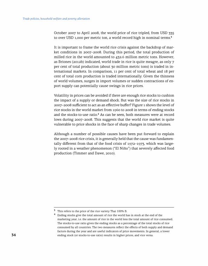
34
Trade policies, household welfare and poverty alleviation
October 2007 to April 2008, the world price of rice tripled, from USD 335 to over USD 1,000 per metric ton, a world record high in nominal terms.3
It is important to frame the world rice crisis against the backdrop of mar-ket conditions in 2007–2008. During this period, the total production of milled rice in the world amounted to 432.6 million metric tons. However, as Briones (2012b) indicated, world trade in rice is quite meagre, as only 7 per cent of total production (about 30 million metric tons) is traded in in-ternational markets. In comparison, 11 per cent of total wheat and 18 per cent of total corn production is traded internationally. Given the thinness of world volumes, surges in import volumes or sudden contractions of ex-port supply can potentially cause swings in rice prices.
Volatility in prices can be avoided if there are enough rice stocks to cushion the impact of a supply or demand shock. But was the size of rice stocks in 2007–2008 sufficient to act as an effective buffer? Figure 1 shows the level of rice stocks in the world market from 1960 to 2008 in terms of ending stocks and the stocks-to-use ratio.4 As can be seen, both measures were at record lows during 2007–2008. This suggests that the world rice market is quite vulnerable to price shocks in the face of sharp changes in trade volumes.
Although a number of possible causes have been put forward to explain the 2007–2008 rice crisis, it is generally held that the cause was fundamen-tally different from that of the food crisis of 1972–1973, which was large-ly rooted in a weather phenomenon (“El Niño”) that severely affected food production (Timmer and Dawe, 2010).
3 This refers to the price of the rice variety Thai 100% B. 4 Ending stocks give the total amount of rice the world has in stock at the end of the marketing year, i.e. the amount of rice in the world less the total amount of rice consumed. The stocks-to-use ratio gives the ending stocks as a percentage of the total stocks of rice consumed by all countries. The two measures reflect the effects of both supply and demand factors during the year and are useful indicators of price movements. In general, a lower ending stock (or stocks-to-use ratio) results in higher prices, and vice versa.

35
Phi
lipp
ines
Distributional impact of the 2008 rice crisis in the Philippines
Figure 1 World rice market – Ending stocks and stocks-to-use ratio, 1960–2012
160
140
120
100
80
60
40
20
0
Mill
ions
of
met
ric
tons
Per
cent
40
35
30
25
20
15
10
5
0
1960
1963
1966
1969
1972
1975
1978
1981
1984
1987
1990
1993
1996
1999
2002
2005
2008
2011
Source: Authors’ estimations, based on USDA (2013).Note: LHS stands for left-hand scale, RHS for right-hand scale.
No supply shock of such proportions took place in 2007–2008. Rather than a natural disaster, the world market was hit by artificial scarcity (Timmer, 2010) caused by a confluence of low global rice stocks, hoarding of rice supplies by consumers, farmers, and traders, and ad hoc responses of gov-ernments to fears of impending rice shortages. When traditional rice-ex-porting countries like India and Vietnam instituted export bans, a spirit of uncertainty pervaded the international rice markets. Importers, on the oth-er hand, jostled to stabilize their own markets as international rice sup-plies rapidly thinned. Sarris (2010) stated that when market agents realize that buffers in global markets are too low to assure adequate supply flows, they start to behave atomistically to ensure the supply flow in their own domestic markets. This “herd” behaviour creates panic buying and hoard-ing, even when the underlying conditions do not justify it, and thus leads to price spikes. Such surge in prices was graphically manifested in the global rice crisis of 2007–2008.
Dawe and Slayton (2010) commented that the 2007–2008 rice crisis was not a failure of the free market to deliver optimal outcomes, but rather that government decisions were instrumental in fanning the crisis. Because the international rice market is thin, and governments play a large role in in-ternational trade, the market is particularly vulnerable to such panics and uncertainty.
― Ending stocks (LHS)
― Stocks-to-use ratio (RHS)

36
Trade policies, household welfare and poverty alleviation
4 Methodology and summary statistics
The methodology of this study closely follows the study by Deaton (1989) on the distributional consequences of rice price changes in Thailand fol-lowing adjustments to an export tax. During the 2008 rice crisis, rice pric-es in the Philippines rose significantly. Given the standard framework, the welfare implications of the price change depend on whether the household is a net producer or a net consumer of rice.
The empirical methods used in this study allow for assessing distribu-tional effects by identifying which households are affected by a shock in the price of rice. This assessment involves three steps. First, we provide a descriptive analysis of household characteristics through expenditure distributions of households across different groups: the total sample, fe-male- and male-headed households, urban and rural households, and ag-ricultural and non-agricultural households. This allows for assessing the well-being of various groups of households.
Second, we use non-parametric regressions to evaluate the relationship between per capita expenditure of households and the level of rice con-sumption and production. The objective is to evaluate how a change in the price of rice affects households, based on whether the households are net producers or net consumers of rice.
Third, we simulate the effects of the rice crisis on household welfare. While it is important to analyse the different channels through which households are affected, this study focuses on the price effects of the rice crisis. In particular, for each household, we estimate the compensating variation, which is the additional amount of money the household needs to remain at the same welfare level as before the crisis. The estimation incorporates the average price of rice before and after the 2008 crisis, and the difference in the rate of increase of the price of rice at the farm gate and retail levels. In addition, a non-parametric regression is used to examine the welfare ef-fects of price changes triggered by the rice crisis on households with dif-ferent levels of per capita expenditure.
Following the standard methodology for the analysis of the distribution-al impact of price changes, this study uses household data from the FIES,5 which is a nationwide survey of households undertaken every three years by the National Statistics Office. The aim of the survey is to gather data on family income and expenditure that are representative of the country and

37
Phi
lipp
ines
Distributional impact of the 2008 rice crisis in the Philippines
its administrative regions. Information gathered in this survey is used by the national authorities to construct the consumer price index and to as-sess human development, poverty, and standards of living, among others.
This study uses the 2009 FIES, since it is closer to the crisis year than the 2006 FIES. The 2009 FIES included the country’s 17 administrative regions as its sampling domain and made use of an area sample design. The re-gions were stratified into non-overlapping subgroups called “strata”,6 with primary sampling units defined as a barangay7 or a combination of ba-rangays consisting of at least 500 households.
Table 1 shows the distribution of the households surveyed in 2009, disag-gregated by gender of the household head, urbanity, agricultural house-hold indicator, and administrative region. A total of 38,400 households were surveyed in the 2009 FIES. Note that a larger percentage of the sam-ple is male-headed, rural, and non-agricultural.
5 More details on the FIES are available at: http://www.census.gov.ph/article/technical-notes- family-income-and-expenditure-survey-fies. 6 The fact that 452 strata only contain a single sampling unit may lead to missing standard errors in the estimations. 7 A barangay is the smallest administrative unit in the Philippines. It corresponds roughly to a village or a district.
Household group Number of observations
Share in the sample (per cent)
All households 38,400 100.00
Gender of household head
Male 30,585 79.65
Female 7,815 20.35
Urbanity
Urban 17,335 45.14
Rural 21,065 54.86
Agricultural household indicator
Agricultural 9,944 25.90
Non-agricultural 28,456 74.10
Table 1 Structure of the sample
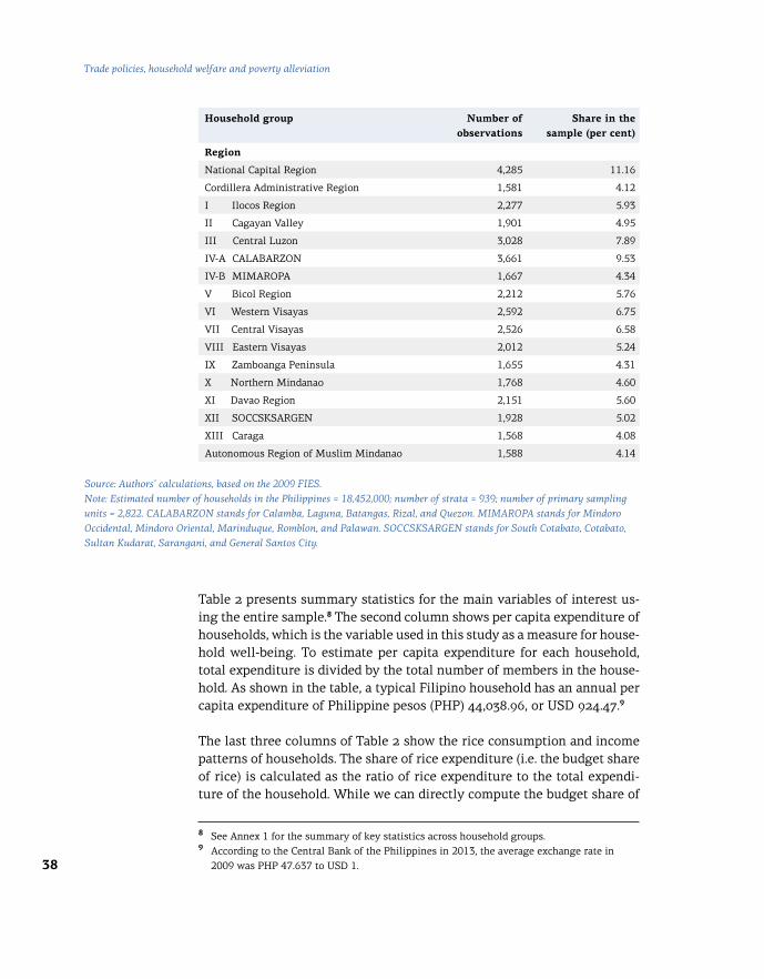
38
Trade policies, household welfare and poverty alleviation
Household group Number of observations
Share in the sample (per cent)
Region
National Capital Region 4,285 11.16
Cordillera Administrative Region 1,581 4.12
I Ilocos Region 2,277 5.93
II Cagayan Valley 1,901 4.95
III Central Luzon 3,028 7.89
IV-A CALABARZON 3,661 9.53
IV-B MIMAROPA 1,667 4.34
V Bicol Region 2,212 5.76
VI Western Visayas 2,592 6.75
VII Central Visayas 2,526 6.58
VIII Eastern Visayas 2,012 5.24
IX Zamboanga Peninsula 1,655 4.31
X Northern Mindanao 1,768 4.60
XI Davao Region 2,151 5.60
XII SOCCSKSARGEN 1,928 5.02
XIII Caraga 1,568 4.08
Autonomous Region of Muslim Mindanao 1,588 4.14
Source: Authors’ calculations, based on the 2009 FIES.Note: Estimated number of households in the Philippines = 18,452,000; number of strata = 939; number of primary sampling units = 2,822. CALABARZON stands for Calamba, Laguna, Batangas, Rizal, and Quezon. MIMAROPA stands for Mindoro Occidental, Mindoro Oriental, Marinduque, Romblon, and Palawan. SOCCSKSARGEN stands for South Cotabato, Cotabato, Sultan Kudarat, Sarangani, and General Santos City.
Table 2 presents summary statistics for the main variables of interest us-ing the entire sample.8 The second column shows per capita expenditure of households, which is the variable used in this study as a measure for house-hold well-being. To estimate per capita expenditure for each household, total expenditure is divided by the total number of members in the house-hold. As shown in the table, a typical Filipino household has an annual per capita expenditure of Philippine pesos (PHP) 44,038.96, or USD 924.47.9
The last three columns of Table 2 show the rice consumption and income patterns of households. The share of rice expenditure (i.e. the budget share of rice) is calculated as the ratio of rice expenditure to the total expendi-ture of the household. While we can directly compute the budget share of
8 See Annex 1 for the summary of key statistics across household groups. 9 According to the Central Bank of the Philippines in 2013, the average exchange rate in 2009 was PHP 47.637 to USD 1.

39
Phi
lipp
ines
Distributional impact of the 2008 rice crisis in the Philippines
10 Data on the level of rice production per region were obtained from the Bureau of Agricultural Statistics (2013).
rice from the 2009 FIES dataset, we cannot do the same for the rice income share because of the absence of data on income from rice production at the household level. As a proxy for income from rice, we use the household in-come from crop production net of the expenses from crop farming. To ad-just for regional differences in the prevalence of rice production, we adjust the data by imputing a factor that is the share of rice in the total value of crop production per region. To illustrate, we define rice income using the following equation:
rice income = k * net income from crop production (1)
where k is the ratio of rice production and total crop production in the re-gion.10 On average, a household spends 13.1 per cent of its budget on rice and earns 3.59 per cent of its total income from rice farming. One limita-tion of this method of constructing rice income is that it assumes the ex-istence of a representative farmer.
Finally, the net income share of rice is calculated per household by taking the difference between its share of rice income and its share of rice expend-iture. The average net income share of rice is –9.52 per cent, which means that a typical Filipino household is a net consumer of rice.
Table 2 Summary of key statistics
Per capita expenditure
(PHP)
Budget share of rice
(per cent)
Income share of rice
(per cent)
Net income share of rice
(per cent)
25th percentile 17,895.60 5.98 0.00 –15.13
Mean 44,038.96 13.10 3.59 –9.52
75th percentile 50,701.67 18.21 1.83 –4.18
Standard deviation 53,086.21 9.29 8.24 10.77
Source: Authors’ calculations, based on the 2009 FIES.Note: Estimated number of households in the Philippines = 18,452,000; number of strata = 939; number of primary sampling units = 2,822.
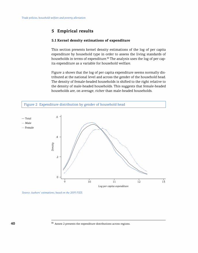
40
Trade policies, household welfare and poverty alleviation
5 Empirical results
5.1 Kernel density estimations of expenditure
This section presents kernel density estimations of the log of per capita expenditure by household type in order to assess the living standards of households in terms of expenditure.11 The analysis uses the log of per cap-ita expenditure as a variable for household welfare.
Figure 2 shows that the log of per capita expenditure seems normally dis-tributed at the national level and across the gender of the household head. The density of female-headed households is shifted to the right relative to the density of male-headed households. This suggests that female-headed households are, on average, richer than male-headed households.
Figure 2 Expenditure distribution by gender of household head
0
.2
.4
.6
Den
sity
9 10 11 12 13
Log per capita expenditure
Source: Authors’ estimations, based on the 2009 FIES.
11 Annex 2 presents the expenditure distributions across regions.
― Total
― Male
Female

41
Phi
lipp
ines
Distributional impact of the 2008 rice crisis in the Philippines
It is important to see this result in the context of the relationship between gender and poverty. The literature review by Lampietti and Salker (2000) reveals that there is a significant variation in the nature and extent of gen-der inequality across countries, thus making it impossible to generalize the welfare disparities between women and men. Marcoux (1998), Chant (1997), and Rosenhouse (1994) stress that evidence on the poverty status of female-headed households in comparison to male-headed households is ambiguous. Moreover, they argue that the evidence surrounding the in-cidence of poverty in female-headed households is country-specific and case-specific. In Viet Nam and Thailand, for example, Klasen et al. (2011) find that female-headed families are better off than male-headed families in terms of current consumption, while UNCTAD (2011) reports that this is not the case in Cape Verde.
The poverty status of female households in the Philippines clearly differs from that of Cape Verde, as shown by several studies. Schelzig (2005) finds that both the incidence and the severity of poverty among female-head-ed families in the Philippines are lower. Balatibat and Nierras (2005) find that female-headed families are not poorer than male-headed households. According to UNESCAP (2010), poverty among female-headed house-holds was consistently 14 to 15 percentage points lower than that of the male-headed households during the period from 1985 to 1994. Bernardino (2011) corroborates these findings by asserting that 42 per cent of fe-male-headed households in the Philippines belong to the richest 30 per cent of the income distribution, while only one-fifth belong to the poor-est 20 per cent.
Chant (2006) conducted one-on-one interviews and focus groups with 223 respondents from low-income groups in three countries – the Gambia, Costa Rica, and the Philippines – between 2003 and 2005. The finding was that poverty is more likely to afflict male-headed households than female-head-ed households in the case of the Gambia and the Philippines. Intal (1994) attributes this to higher educational attainment, smaller family size, and female-biased employment demand in the formal sector, particularly in the export sector. The findings with regard to the differences in distribu-tion of per capita expenditure for male- and female-headed households in 2009 in the current study are therefore consistent with the literature.
Figure 3 presents the expenditure distribution of households by level of ur-banity. It shows that the distribution of urban households relative to that of rural households is shifted to the right. This means that, on average, ur-ban households are richer than rural households. It is not difficult to im-agine why this is so, since there are more opportunities to earn a living in

42
Trade policies, household welfare and poverty alleviation
urban areas. Also, the distribution for rural households is right skewed, in-dicating that a large portion of rural households are poor.
Figure 3 Expenditure distribution by level of urbanity
Source: Authors’ estimations, based on the 2009 FIES.
Finally, Figure 4 presents the expenditure distribution of agricultural and non-agricultural households. On average, non-agricultural households are relatively richer than agricultural households, as evidenced by the plot lines in the figure. Moreover, the right skewedness of the distribution of agricultural households suggests that the majority of agricultural house-holds have low levels of expenditure.
0
.2
.4
.6
Den
sity
9 10 11 12 13
Log per capita expenditure
.8― Total
― Rural
Urban

43
Phi
lipp
ines
Distributional impact of the 2008 rice crisis in the Philippines
Source: Authors’ estimations, based on the 2009 FIES.
Figure 4 Expenditure distribution by agricultural household indicator
5.2 Non-parametric regressions
This section presents non-parametric regressions on the log of per capi-ta expenditure of the following: (a) the share of rice in total expenditure, (b) the share of rice in total income, and (c) the net share of rice in total income. These regressions will help explain the distributional effects of shocks in the price of rice while taking into account the disparities in liv-ing standards based on the gender of the household head, the level of ur-banity, and the agricultural/non-agricultural household indicator.
Figure 5 presents the result for the share of rice in total expenditure. The share of rice in total expenditure at the left tail of the distribution is al-most 25 per cent and decreases significantly as one moves from poorer to relatively better-off households. This behaviour is expected and consistent with Engel’s Law, as it implies that the budget shares of relatively more ex-pensive food items and other non-food items increase with the level of ex-penditure. Also, the budget share of rice is slightly lower for female-headed households, but the difference vanishes for richer households.
Reyes et al. (2009) show that the share of rice in total expenditure decreas-es as income increases. Their findings show that there are more net rice
0
.2
.4
.6
Den
sity
9 10 11 12 13
Log per capita expenditure
.8 ― Total
― Agricultural
Non-agricultural

44
Trade policies, household welfare and poverty alleviation
consumers (84.7 per cent of households) than there are net producers (12.8 per cent) in the Philippines, thus indicating that there are more house-holds that will be negatively affected by the increase in rice prices.12 They obtain the same results when the data are disaggregated by urbanity, in-come decile, and region.13
Figure 5 Budget share of rice and per capita expenditure by gender of household head
Source: Authors’ estimations, based on the 2009 FIES.
In terms of rice production of households, the share of rice in total income declines with the level of well-being, as evidenced in Figure 6. However, on average, rice income is much lower in female-headed households than in male-headed households. This suggests that female-headed households may have other sources of income aside from rice production. Note that the gender-related difference is most pronounced for poor households and becomes smaller as expenditure increases.
12 In contrast to our constructed indicator for the income share of rice, Reyes et al. (2009) used the actual rice income from the 2006 FIES. However, this variable is not readily available to the public in the 2009 FIES.. 13 Annex 3 presents the non-parametric regressions on the log of per capita expenditure of the share of rice in total expenditure and the share of rice in total income by level of urbanity and agricultural household indicator.
0
.05
.15
.2
Bud
get
shar
e
9 10 11 12 13Log per capita expenditure
.25
.1
― Total
― Male-headed
Female-headed

45
Phi
lipp
ines
Distributional impact of the 2008 rice crisis in the Philippines
Figure 6 Income share of rice and per capita expenditure by gender of household head
Source: Authors’ estimations, based on the 2009 FIES.
In order to see the short-term impact of a rice price shock on households with different expenditure levels, we estimate a non-parametric regression of the net income share of rice, which is the equivalent of the net bene-fit ratio (NBR) of Deaton (1989). Furthermore, to see the difference in con-sumption and production patterns across household types, we present the regressions separately by gender of the household head, level of urbanity, and agricultural household indicator.
The result by gender of the household head is presented in Figure 7. On av-erage, the net income share of rice stands at –9.52 per cent, indicating that Filipino households are mostly net rice consumers. On average, the net share of rice in total income for both male- and female-headed households is negative across all levels of per capita expenditure. For households at the lower tail of the income distribution, net rice income is approximately –20 per cent and becomes less negative as one moves from poorer to rich-er households. This suggests that an increase in the price of rice is high-ly regressive; that is, an increase in the price of rice would hurt the poor more. Moreover, we can see that at each level of per capita expenditure, fe-male-headed households have a slightly lower (i.e. more negative) net in-come share of rice compared to male-headed households.
― Total
― Male-headed
Female-headed
0
.02
.04
.06
Inco
me
shar
e
Log per capita expenditure
.08
9 10 11 12 13
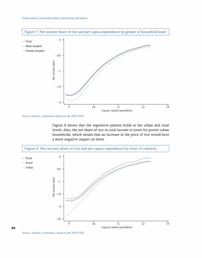
46
Trade policies, household welfare and poverty alleviation
Figure 8 shows that the regressive pattern holds at the urban and rural levels. Also, the net share of rice in total income is lower for poorer urban households, which means that an increase in the price of rice would have a more negative impact on them.
Figure 7 Net income share of rice and per capita expenditure by gender of household head
Figure 8 Net income share of rice and per capita expenditure by level of urbanity
Source: Authors’ estimations, based on the 2009 FIES.
Source: Authors’ estimations, based on the 2009 FIES.
–.2
–.25
–.2
–.15
–.15
–.1
–.1
–.05
–.05
Net
inco
me
shar
eN
et in
com
e sh
are
Log per capita expenditure
Log per capita expenditure
0
0
9
9
10
10
11
11
12
12
13
13
― Total
― Male-headed
Female-headed
― Total
― Rural
Urban

47
Phi
lipp
ines
Distributional impact of the 2008 rice crisis in the Philippines
Source: Authors’ estimations, based on the 2009 FIES.
The regression for non-agricultural households in Figure 9 is similar to that for urban house-holds, but slightly more negative. Interestingly, while the net income shares of agricultural households at lower levels of per capita expenditure are negative, those at higher levels of per capita expenditure are positive. This means that poorer agricultural households are more like-ly to be net consumers of rice and thus would be worse off if the price of rice were to increase. Conversely, richer agricultural households tend to be net producers of rice and thus would be better off if the price of rice were to increase.
Figure 9 Net income share of rice and per capita expenditure by agricultural household indicator
These findings for the agricultural and non-agricultural cases are consist-ent with Fujii (2013), who finds that agricultural households are less vul-nerable than non-agricultural households. In general, poorer households are more vulnerable than wealthier ones to food inflation.
6 Simulations
The non-parametric regression results presented above are useful for de-scribing the profile of households that are likely to be vulnerable to shocks in rice prices. However, they do not allow for seeing the extent of the im-pact of the 2008 rice crisis on household welfare. That is, the previous re-gressions do not account for the actual price increase and the imperfect transmission of the price increase during that rice crisis episode.
–.2
–.1
0
.1
Net
inco
me
shar
e
Log per capita expenditure9 10 11 12 13
― Total
― Agricultural
Non-agricultural

48
Trade policies, household welfare and poverty alleviation
6.1 Imperfect transmission of prices during the 2008 rice crisis
Figure 10 presents the trend in domestic rice prices in PHP from 2007 to 2009.14 The trends are broadly similar at the wholesale, retail, and farm gate levels, but farm gate prices are significantly lower than the other two, which are similar to each other.
Following Balisacan et al. (2010), we divide the period considered into three phases: pre-crisis (January 2007 to February 2008), crisis (March 2008 to September 2008), and post-crisis (October 2008 to August 2009). In the pre-crisis phase, the prices averaged PHP 22.54 per kilogram (kg) at the retail level, PHP 20.82 per kg at the wholesale level, and PHP 11.32 per kg at the farm gate level. During the crisis, average retail prices of rice rose by 39.77 per cent (to PHP 31.50 per kg), wholesale prices increased by 40.47 per cent (to PHP 29.25 per kg), and farm gate prices by 34.12 per cent (to PHP 15.18 per kg). At the peak in June 2008, retail prices were higher by 51.78 per cent, wholesale prices by 54.97 per cent and farm gate prices by 59.05 per cent than the prices in February 2008.15 Prices started to decline in July and stabilized in October 2008. Note that the prices in the post-cri-sis phase were higher relative to those in the pre-crisis phase.
Source: Authors’ estimations, based on data from the Bureau of Agricultural Statistics (2013).Note: Wholesale and retail prices – regular milled rice; farm gate price – palay (paddy) other variety, dry (converted to 14 per cent moisture content).
Figure 10 Monthly trends in retail, wholesale and farm gate rice prices, January 2007 – August 2009 (PHP per kg)
0
10
5
25
20
15
30
PH
P p
er k
g
40
35
Jan
2007
Jan
2008
Jan
2009
Mar
200
7
Mar
200
8
Mar
200
9
May
200
7
May
200
8
May
200
9
Jul
2007
Jul
2008
Jul
2009
Sep
2007
Sep
2008
Nov
200
7
Nov
200
8
― Retail
― Wholesale
Farm gate

49
Phi
lipp
ines
Distributional impact of the 2008 rice crisis in the Philippines
In analysing the distributional impact of the actual price shock of 2008, we incorporate the imperfect transmission of price from the pre-crisis phase (January 2007 to February 2008) to the crisis phase (March 2008 to September 2008).
Let the rate of increase of rice prices at the retail level be x and the rate of increase at the farm gate level be y. Suppose that in a certain geographical region, the former exceeds the latter, that is, x > y. Because the difference in the price increase rates is already known ex post, one can establish that the magnitude of y is a fraction of x, say, y = ax where a is a constant. In the next subsection, we will include this constant a as a scale effect when we compute the net difference between the share of rice in the food budget and in total household income.
Table 3 shows the average rate of change in national and regional farm gate and retail prices during the pre-crisis and crisis phases. In the far right column, which gives the ratio of the average rates of change in farm gate and retail prices, one sees that the ratio is below 1 at the national lev-el. This means that the retail price transmission to farm gate prices was imperfect. In particular, retail prices increased more rapidly than farm gate prices during the rice crisis. Across regions, the transmission varied. For instance, similar to that of the national level, the Caraga, Central Visayas, and Northern Mindanao regions had ratios below 1. However, for the Autonomous Region of Muslim Mindanao, the Cordillera Administrative Region, and Eastern Visayas, the ratio was above 1, which means that in those regions, the increase in farm gate prices was greater than the in-crease in retail prices.
14 Data on rice prices were collected from the Bureau of Agricultural Statistics, which distinguishes three types of rice prices: farm gate, wholesale, and retail. Such data series are available from 1990 to 2012. For the trends at the wholesale and retail levels, we use monthly wholesale and retail prices of regular milled rice, while for the trends at the farm gate level we use the farm gate prices of palay (paddy, other variety, dry). 15 The rice prices at the retail, wholesale, and farm gate levels are nominal. To lend perspective, in June 2008, retail prices were higher by 51.78 per cent compared to February 2008 prices. For the same period, the increase in the consumer price index was 5.15 per cent.

50
Trade policies, household welfare and poverty alleviation
Table 3 Average rate of change of national and regional farm gate and retail prices during the 2008 rice crisis
Region Change in farm gate price
(per cent), y
Change in retail price
(per cent), x
a = y/x
All regions 34.12 39.77 0.8580
National Capital Region .. 44.95 1§
Cordillera Administrative Region 47.16 43.58 1.0821
I Ilocos Region 37.77 45.72 0.8261
II Cagayan Valley 37.64 42.81 0.8793
III Central Luzon 36.39 42.71 0.8520
IV–A CALABARZON 36.91 42.70 0.8642
IV–B MIMAROPA 32.62 37.67 0.8660
V Bicol Region 33.43 39.66 0.8431
VI Western Visayas 27.69 33.48 0.8271
VII Central Visayas 28.14 41.68 0.6751
VIII Eastern Visayas 40.17 39.17 1.0257
IX Zamboanga Peninsula 31.16 40.57 0.7681
X Northern Mindanao 30.78 41.32 0.7448
XI Davao Region 33.62 39.84 0.8438
XII SOCCSKSARGEN 25.49 33.71 0.7562
XIII Caraga 24.86 39.93 0.6227
Autonomous Region of Muslim Mindanao
37.89 33.98 1.1152
Source: Authors’ calculations, based on the average farm gate prices of palay (paddy, other variety, dry) and average retail prices of rice (regular milled rice) from the Bureau of Agricultural Statistics (2013).Note: Prices changes refer to the growth rate of prices between the pre-crisis phase (January 2007 to February 2008) and the crisis phase (March 2008 to September 2008).Two dots (..) indicate that data are not available.§ Data on farm gate prices for the National Capital Region are not available as the volume of rice production in this region is negligible. We therefore assume that at any point in time there is no disparity between the retail and farm gate prices in the National Capital Region.
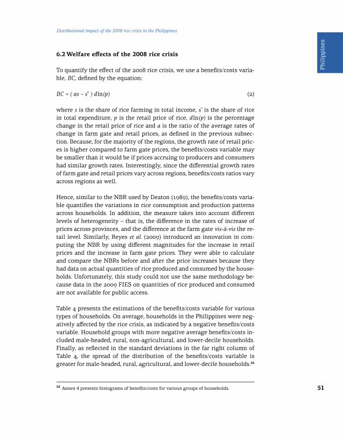
51
Phi
lipp
ines
Distributional impact of the 2008 rice crisis in the Philippines
6.2 Welfare effects of the 2008 rice crisis
To quantify the effect of the 2008 rice crisis, we use a benefits/costs varia-ble, BC, defined by the equation:
BC = ( as – s* ) d ln(p) (2)
where s is the share of rice farming in total income, s* is the share of rice in total expenditure, p is the retail price of rice, d ln(p) is the percentage change in the retail price of rice and a is the ratio of the average rates of change in farm gate and retail prices, as defined in the previous subsec-tion. Because, for the majority of the regions, the growth rate of retail pric-es is higher compared to farm gate prices, the benefits/costs variable may be smaller than it would be if prices accruing to producers and consumers had similar growth rates. Interestingly, since the differential growth rates of farm gate and retail prices vary across regions, benefits/costs ratios vary across regions as well.
Hence, similar to the NBR used by Deaton (1989), the benefits/costs varia-ble quantifies the variations in rice consumption and production patterns across households. In addition, the measure takes into account different levels of heterogeneity – that is, the difference in the rates of increase of prices across provinces, and the difference at the farm gate vis-à-vis the re-tail level. Similarly, Reyes et al. (2009) introduced an innovation in com-puting the NBR by using different magnitudes for the increase in retail prices and the increase in farm gate prices. They were able to calculate and compare the NBRs before and after the price increases because they had data on actual quantities of rice produced and consumed by the house-holds. Unfortunately, this study could not use the same methodology be-cause data in the 2009 FIES on quantities of rice produced and consumed are not available for public access.
Table 4 presents the estimations of the benefits/costs variable for various types of households. On average, households in the Philippines were neg-atively affected by the rice crisis, as indicated by a negative benefits/costs variable. Household groups with more negative average benefits/costs in-cluded male-headed, rural, non-agricultural, and lower-decile households. Finally, as reflected in the standard deviations in the far right column of Table 4, the spread of the distribution of the benefits/costs variable is greater for male-headed, rural, agricultural, and lower-decile households.16
16 Annex 4 presents histograms of benefits/costs for various groups of households.

52
Trade policies, household welfare and poverty alleviation
Table 4 Welfare effects of the 2008 rice crisis on various groups of households
Household group25th
percentileMean
75th percentile
Standard deviation
All households –0.0614 –0.0400 –0.0183 0.0406
Gender of HH head
Male –0.0634 –0.0407 –0.0189 0.0422
Female –0.0532 –0.0372 –0.0166 0.0338
Urbanity
Urban –0.0494 –0.0358 –0.0182 0.0294
Rural –0.0734 –0.0441 –0.0185 0.0490
Agricultural HH indicator
Agricultural –0.0786 –0.0360 0.0035 0.0625
Non-agricultural –0.0572 –0.0411 –0.0201 0.0313
National income decile
1 –0.0883 –0.0545 –0.0189 0.0524
2 –0.0880 –0.0571 –0.0288 0.0485
3 –0.0831 –0.0549 –0.0318 0.0456
4 –0.0748 –0.0498 –0.0300 0.0433
5 –0.0677 –0.0465 –0.0298 0.0390
6 –0.0574 –0.0399 –0.0263 0.0353
7 –0.0482 –0.0329 –0.0229 0.0322
8 –0.0398 –0.0280 –0.0190 0.0265
9 –0.0321 –0.0221 –0.0150 0.0232
10 –0.0207 –0.0140 –0.0090 0.0186
Region
National Capital Region –0.0331 –0.0249 –0.0139 0.0149
Cordillera Administrative Region
–0.0484 –0.0241 –0.0101 0.0495
I Ilocos Region –0.0727 –0.0455 –0.0219 0.0437
II Cagayan Valley –0.0560 –0.0128 0.0269 0.0614
III Central Luzon –0.0531 –0.0294 –0.0186 0.0475
IV–A CALABARZON –0.0521 –0.0389 –0.0205 0.0261
IV–B MIMAROPA –0.0731 –0.0443 –0.0188 0.0457
V Bicol Region –0.0729 –0.0486 –0.0222 0.0394
VI Western Visayas –0.0706 –0.0479 –0.0243 0.0357
VII Central Visayas –0.0667 –0.0462 –0.0194 0.0438
VIII Eastern Visayas –0.0851 –0.0544 –0.0238 0.0466
IX Zamboanga Peninsula
–0.0746 –0.0442 –0.0122 0.0501

53
Phi
lipp
ines
Distributional impact of the 2008 rice crisis in the Philippines
Household group25th
percentileMean
75th percentile
Standard deviation
X Northern Mindanao
–0.0778 –0.0526 –0.0231 0.0415
XI Davao Region -0.0662 -0.0475 -0.0248 0.0331
XII SOCCSKSARGEN -0.0684 -0.0457 -0.0224 0.0352
XIII Caraga -0.0950 -0.0697 -0.0412 0.0414
Autonomous Region of Muslim Mindanao
-0.0546 -0.0317 -0.0041 0.0389
Source: Authors’ calculations, based on the 2009 FIES and Bureau of Agricultural Statistics (2013). Note: HH stands for household.
However, the differences across groups in this table only reflect the effects of the price changes owing to differences in per capita expenditure across groups, differences in rice production and consumption patterns, and in price increases across regions. Therefore, we cannot use this table to com-pare welfare effects across groups of households, such as between male- and female-headed households, at the same level of per capita expenditure. In the following section, the distributional analysis takes into account the well-being of the household – a factor that could determine whether a household would gain or lose from the rice price shock.
6.3 Benefits/costs and levels of household expenditure
It is also important to look at the distribution of the benefits/costs in dif-ferent categories as measured by per capita expenditure. This yields re-sults that are comparable to the regressions of the net income share of rice in Section 5.
Figure 11 shows the non-parametric regression results by gender of the household head. As expected, the benefits/costs variable is negative throughout the distribution and becomes less negative with higher ex-penditure levels. This means that higher prices due to the 2008 rice cri-sis hurt the poor the most. Moreover, the benefits/costs for female-headed households are lower than the benefits/costs for male-headed households. The effect of the 2008 rice crisis therefore seems to have been more detri-mental to the female-headed households. The reason for this result is that female-headed households are more likely the net consumers of rice at all levels of per capita expenditure, as seen in Figure 7.

54
Trade policies, household welfare and poverty alleviation
Figure 11 Benefits/costs and per capita expenditure by gender of household head
Figure 12 Benefits/costs and per capita expenditure by level of urbanity
Source: Authors’ estimations, based on the 2009 FIES and Bureau of Agricultural Statistics (2013).
Source: Authors’ estimations, based on the 2009 FIES and Bureau of Agricultural Statistics (2013).
As seen in Figure 12, the regressions estimated for urban and rural house-holds likewise display a regressive trend. Urban households, on average, have a more negative benefits/costs variable across the spectrum. This sug-gests that urban households were worse off relative to the rural households.
–.08
–.1
–.08
–.06
–.06
–.04
–.04
–.02
–.02
Ben
efits
/cos
tsB
enefi
ts/c
osts
Log per capita expenditure
Log per capita expenditure
0
0
9
9
10
10
11
11
12
12
13
13
― Total
― Male-headed
Female-headed
― Total
― Rural
Urban

55
Phi
lipp
ines
Distributional impact of the 2008 rice crisis in the Philippines
Figure 13 Benefits/costs and per capita expenditure by agricultural household indicator
Source: Authors’ estimations, based on the 2009 FIES and Bureau of Agricultural Statistics (2013).
Finally, Figure 13 shows that across levels of expenditure, non-agricultural households have a lower benefits/costs variable, suggesting that they were more adversely affected than agricultural households. In addition, note that in the regression for agricultural households, households at the right tail of the distribution have a positive benefits/costs variable. This means that richer agricultural households gained from the rice crisis, as they are more likely the net producers of rice.
6.4 Who are the gainers and losers from the 2008 rice crisis?
Following Reyes et al. (2009), we use the plus or minus sign of the house-hold benefits/costs variable, BC, to assess how the welfare of households has changed due to the 2008 rice crisis. If BC > 0, the household is defined as better off from the increase in the rice price and thus is a “gainer” in the rice crisis. Conversely, if BC < 0, the household is defined as worse off from the increase in the rice price and thus is a “loser” in the rice crisis. Note that the identification of gainers and losers does not take into account the magnitude of the gain or loss, but just the sign.
Table 5 presents the breakdown of the population in each sub-group into unaffected, gainers, and losers. Among households in the Philippines, 91 per cent were losers in the rice crisis while only 8.4 per cent were gain-ers and 0.6 per cent were unaffected. Regardless of the type of household,
–.1
–.05
0
.05
Ben
efits
/cos
ts
Log per capita expenditure9 10 11 12 13
― Total
― Agricultural
Non-agricultural

56
Trade policies, household welfare and poverty alleviation
those who were adversely affected by the rice crisis clearly outnumbered those who were better off. This result is consistent with the result of Reyes et al. (2009), who, based on the change in the NBR due to rice price chang-es, found that 85.5 per cent of households in the Philippines were negative-ly affected while only 12.1 per cent benefited during the crisis.
The far right column of Table 5 shows the proportions of households de-fined as losers in the rice crisis. As shown, female-headed, rural, non-ag-ricultural, and higher-income households tend to have higher shares of losers relative to their counterparts. These results seem contradictory to the results in Table 4. Accordingly, based on the average values of benefits/costs, the better-off groups include female-headed, urban, and higher-in-come households. However, the distribution of benefits/costs in Annex 4 shows that losers in the female-headed, urban, and higher-income groups, although higher in terms of share, tend to have higher (i.e. less negative) values of benefits/costs variable relative to the losers in the male-headed, rural, and lower-income groups. One can also note from the standard de-viation of the benefits/costs in Table 4 that the spread of the distribution of the variable for households in the lower-income brackets is wider, thus making it possible to have a higher share of households that end up as gainers from the price change (see Figure A4.4 in Annex 4).
Note also that the proportions of gainers among rural households (14.34 per cent) and agricultural households (26.59 per cent) were considera-ble. Moreover, there were a number of gainers in the lower-income de-ciles and in regions such as the Cagayan Valley, Autonomous Region of Muslim Mindanao, Cordillera Administrative Region, and the Zamboanga Peninsula. This suggests that there are a number of net sellers of rice in these groups.
Table 5 Proportion of unaffected, gainers and losers in the 2008 rice crisis by various groups of households (per cent)
Household group Unaffected Gainers Losers
All households 0.6 8.4 91.0
Gender of household head
Male 0.52 9.55 89.93
Female 0.86 4.13 95.01
Urbanity
Urban 0.58 2.42 97.00
Rural 0.61 14.34 85.05

57
Phi
lipp
ines
Distributional impact of the 2008 rice crisis in the Philippines
Household group Unaffected Gainers Losers
Agricultural household indicator
Agricultural 0.39 26.59 73.02
Non-agricultural 0.65 3.08 96.27
National income decile
1 2.34 15.31 82.35
2 0.76 12.38 86.86
3 0.43 10.36 89.21
4 0.54 10.08 89.38
5 0.31 7.46 92.23
6 0.24 6.82 92.93
7 0.06 6.86 93.08
8 0.66 5.27 94.07
9 0.29 5.03 94.68
10 0.29 4.46 95.26
Region
National Capital Region 0.83 0.10 99.07
Cordillera Administrative Region 0.06 18.68 81.26
I Ilocos Region 0.09 11.91 88.00
II Cagayan Valley 0.42 33.71 65.88
III Central Luzon 0.48 11.24 88.27
IV-A CALABARZON 0.35 1.56 98.09
IV-B MIMAROPA 0.17 12.92 86.90
V Bicol Region 0.27 8.07 91.66
VI Western Visayas 0.47 6.21 93.32
VII Central Visayas 1.57 9.68 88.75
VIII Eastern Visayas 0.22 8.82 90.96
IX Zamboanga Peninsula 1.74 16.76 81.50
X Northern Mindanao 1.18 7.84 90.98
XI Davao Region 0.84 5.23 93.93
XII SOCCSKSARGEN 0.35 7.00 92.65
XIII Caraga 0.25 3.06 96.69
Autonomous Region of Muslim Mindanao
0 22.24 77.76
Source: Authors’ calculations, based on the 2009 FIES and Bureau of Agricultural Statistics (2013). Note: In each row, the values sum to 100.

58
Trade policies, household welfare and poverty alleviation
Table 6 presents, within each category, the breakdown of gainers, losers and unaffected into sub-groups. Most of the losers are located in urban and non-agricultural areas, while the gainers are in rural and agricultural areas. These results are not surprising, as most households in urban and non-agricultural areas tend to be net consumers of rice and those in rural and agricultural areas tend to be net producers of rice. Reyes et al. (2009) also reported a larger proportion of losers in urban areas.
The sub-set of gainers (third column in Table 6) shows that the proportion of households belonging to the lower-income deciles is higher, as they are likely to be net producers of rice.17 Such results are comparable to the find-ings of Reyes et al. (2009).
Looking at regional patterns, most of the losers live in the National Capital Region, the regional grouping of Calamba, Laguna, Batangas, Rizal, and Quezon (CALABARZON), and Central Luzon. This finding is similar to that of Reyes et al. (2009). Most of the gainers live in Central Luzon, Cagayan Valley, Central Visayas, and the Autonomous Region of Muslim Mindanao. In contrast, Reyes et al. (2009) found that most of the gainers were situated in Central Luzon, Ilocos, Western Visayas, and the Cagayan Valley.
Table 6 Distribution of unaffected, gainers and losers in the 2008 rice crisis by various groups of households (per cent)
Household group Unaffected Gainers Losers
Gender of household head
Male 69.29 89.60 77.90
Female 30.71 10.40 22.10
Urbanity
Urban 48.42 14.38 53.12
Rural 51.58 85.62 46.88
Agricultural household indicator
Agricultural 14.80 71.64 18.17
Non-agricultural 85.20 28.36 81.83
National income decile
1 39.54 18.22 9.05
2 12.85 14.73 9.54
17 Balicasan et al. (2010) maintain that, because the poor generally devote higher shares of expenditure to cereals (mainly rice), they tend to be hit harder by a rice crisis. Their finding, however, is not strictly comparable with Table 6 because they did not include rice income in their framework.

59
Phi
lipp
ines
Distributional impact of the 2008 rice crisis in the Philippines
Household group Unaffected Gainers Losers
3 7.24 12.33 9.80
4 9.08 12.00 9.82
5 5.27 8.88 10.14
6 4.11 8.12 10.21
7 1.01 8.17 10.23
8 11.17 6.28 10.34
9 4.89 5.98 10.40
10 4.83 5.30 10.47
Region
National Capital Region 18.71 0.16 14.52
Cordillera Administrative Region 0.17 3.88 1.56
I Ilocos Region 0.81 7.72 5.27
II Cagayan Valley 2.48 14.19 2.56
III Central Luzon 8.98 14.70 10.66
IV-A CALABARZON 7.59 2.42 14.05
IV-B MIMAROPA 0.93 4.92 3.05
V Bicol Region 2.64 5.57 5.84
VI Western Visayas 6.25 5.82 8.07
VII Central Visayas 19.74 8.58 7.26
VIII Eastern Visayas 1.73 4.92 4.68
IX Zamboanga Peninsula 10.53 7.16 3.21
X Northern Mindanao 9.04 4.24 4.55
XI Davao Region 6.78 2.98 4.94
XII SOCCSKSARGEN 2.55 3.61 4.42
XIII Caraga 1.07 0.93 2.71
Autonomous Region of Muslim Mindanao
0.00 8.20 2.65
Source: Authors’ calculations, based on the 2009 FIES and Bureau of Agricultural Statistics (2013).Note: Within each household category, the values in each column sum to 100.
7 Conclusions and policy implications
What was the distributional impact of the 2008 rice crisis in the Philippines? Following the methodology of Deaton (1989), this study mapped out the vulnerability of various household groups to rice price shocks through non-parametric regressions of the net rice share on per capital expendi-ture for different household groups.

60
Trade policies, household welfare and poverty alleviation
At the national level, the measures of the net income share of rice for both male- and female-headed households are negative across all levels of per capita expenditure. The findings also show that for low-income house-holds, net rice income is approximately −20 per cent and becomes less neg-ative as one moves from poorer to richer households. This suggests that an increase in the price of rice is highly regressive – that is, it hurts the poor more, a finding consistent with Reyes et al. (2009) and Fujii (2013). In ad-dition, female-headed households have a slightly lower net income share of rice, suggesting that they are more vulnerable compared to male-head-ed households.
For urban households, the net income share of rice is lower than that for rural households. Furthermore, it is much lower for poorer segments of ur-ban households. This implies that a price shock has a more detrimental ef-fect on the poor in urban areas.
For households in the agricultural sector, the outcome is mixed – poorer agricultural households are net consumers of rice while richer ones are net producers. Hence, price increases hurt poor agricultural households but benefit agricultural households with higher income. On the other hand, as households in the non-agricultural sector are generally net consumers of rice, they are more vulnerable to price shocks compared to households in the agricultural sector.
We carried out simulations on the benefits/costs variable (an indicator for the change in the NBR), given actual price changes at the farm gate and re-tail levels for each household during the 2008 rice crisis. The gainers and losers from the rice crisis could be identified by the sign of the benefits/costs variable (gainers for positive change, losers for negative change). We found that, on average, over 90 per cent of the households in the survey suffered a loss of welfare. The few that gained from the price shock were found mostly in the rural and agricultural sectors.
Although the overwhelming majority at each income decile experienced a loss in welfare, there were relatively more gainers among those in the lower-income deciles than in the higher-income deciles. An explanation is that those belonging to the higher-income deciles are net consumers of rice. Similarly, the majority of the households in all regions suffered a loss in welfare, while the regions with a substantial number of gainers were the Cagayan Valley, Autonomous Region of Muslim Mindanao, Cordillera Administrative Region, and the Zamboanga Peninsula.
61
Phi
lipp
ines
Distributional impact of the 2008 rice crisis in the Philippines
The non-parametric regression of the benefits/costs variable on the log of per capita expenditure provided several results. First, conditional on the level of per capita expenditure, female-headed households are more vul-nerable to changes in rice prices. This means that female-headed house-holds suffered a greater loss of welfare from the crisis.18
Second, conditional on the level of per capita expenditure, the benefits/costs for urban households are lower than for rural households. Such re-sults are not surprising given that urban households are more likely to be net consumers of rice than rural households.19
Third, conditional on the level of per capita expenditure, agricultural households suffered less than non-agricultural households. It is quite ob-vious that the rice producers would be in the agricultural sector and that the urban poor, with very little potential for gains from rice production, would be hit harder.
In the analysis of the impact on households by national income decile, we see that the decreases in the benefits/costs are greater for the lower-in-come deciles. The dispersions are also greater at the lower-income levels than the higher-income ones. Again, one implication is that the poorest of the poor suffer the brunt of the rice crisis.
The profile of gainers and losers is not entirely unexpected, as most house-holds in urban and non-agricultural areas tend to be net consumers of rice, and those in rural and agricultural areas tend to be net producers. Thus, for targeting transfers, Philippine policymakers should be guided by the
18 There appears to be some tension between the absolute values of benefits/costs (Table 4, columns 2–4) and the non-parametric regression results of the net income share of rice and the log of per capita expenditure (Figures 7–9) with regard to identifying the most affected household groups. Considering the relative vulnerability of male- and female- headed households, we can say that, on average, male-headed households experienced a deeper welfare loss (negative benefits/costs) than female-headed ones. However, the benefits/costs variable for male-headed households has a greater dispersion, i.e. a higher standard deviation (Table 4, column 5, and Figure A4.1). In addition, controlling for per capita expenditure, female-headed households are found to have systematically lower benefits/costs (Figure 11). 19 Given the average benefits/costs (Table 4, columns 2–4), rural households appear to suffer a greater loss in welfare than urban households. In addition, the standard deviation of the benefits/costs distribution for rural households is greater, but higher extreme values are found for urban households (Table 4, column 5; Figure A4.2). This implies that some urban households enjoyed particularly high benefits from the price increase, which pushed up the average. However, the proportion of losers in the rural sector is smaller than that in the urban sector (Table 5).

62
Trade policies, household welfare and poverty alleviation
absolute magnitudes of the benefits and costs and by their distribution on the log of per capita expenditure.
By and large, the entire country suffered through the 2008 rice crisis, al-though a minority actually gained. As a short-term measure to help vul-nerable households, Balicasan et al. (2010) advocate the expansion of conditional cash transfers, complemented with a targeted rice subsidy pro-gramme in depressed areas. These safety nets would help avoid hunger and poverty.
Indeed, policymakers are confronted with the challenge of designing an appropriate poverty-alleviating response in the event that a rice crisis oc-curs again. While it is desirable that all affected households have access to assistance programmes such as subsidized rice or conditional cash trans-fers, the government’s resource constraints dictate that there ought to be strategic targeting of beneficiaries. Those that suffer most from the crisis ought to be prioritized by assistance programmes.
However, the effectiveness of assistance programmes is often compro-mised by leakage. Because of poor targeting of the beneficiaries, less-needy households may benefit from government assistance at the expense of more needy ones. Reyes et al. (2009) cite leakage as a reason why cheap subsidized rice from the National Food Authority does not always reach the poor. In addition, the lack of capacity of local governments to accurate-ly identify households for conditional cash transfers limits the effective-ness of the safety net programme of the Department of Social Work and Development.
Hopefully, the findings of this study will help target government relief and safety net programmes in the event of future rice crises. Information about vulnerable household groups from the experience of the 2008 rice crisis in the Philippines may help in the identification of those segments of the population that deserve a higher priority in assistance.
Admittedly, even if this study can help improve the targeting mecha-nism of households that need assistance during food crises, the inade-quacy of the available resources relative to the needs may compromise the effectiveness of such a mechanism. Given the extent of poverty in the Philippines, and the very limited participation of the NFA at present in the market in terms of procurement and buffer stocks, there seems to be very little scope for assistance. Thus, in addition to better targeting, there is a case for considering the expansion of the government budget directed to helping the poor cope with rice crises.
63
Phi
lipp
ines
Distributional impact of the 2008 rice crisis in the Philippines
Balisacan et al. (2010) observe that the past implementation of the NFA’s rice subsidy programme was not cost-effective. Thus, concomitant with expanded budgets for this programme, there is a need for better govern-ance of the NFA.
Social safety net and rice subsidy programmes are only short-term meas-ures, and policymakers also need to look at longer-term solutions. It should be borne in mind that policy options have accompanying costs. Having an idea of the welfare costs resulting from a crisis could help eval-uate such policy options. Our findings about the impact of the 2008 rice crisis indicate that around 90 per cent of households experienced a reduc-tion of welfare to varying degrees. Back-of-the-envelope estimations show that the government needs PHP 803 million worth of measures, such as cash handouts, to bring the welfare of households back to the pre-crisis level.20 In absolute terms, the cost to society is very high. Thus, investing in crafting longer-term policy measures to prevent the crisis from recur-ring is worthwhile.
As a perennial task, policymakers should not abandon initiatives to solve the problem at its core – that is, to improve rice productivity. In fact, be-cause of the structural problems in the rice sector, Balisacan et al. (2010) contend that a rice crisis in the Philippines would have occurred even in the absence of the global price shock. The factors that they cite are similar to those that afflict agriculture and the rural economy in the Philippines in general. One main constraint to Philippine agriculture is the productiv-ity slowdown resulting from the lack of investment in the sector and in support services. Particularly lacking are investments in infrastructure, re-search, and institutions. In addition, assistance to farmers in terms of ex-tension services is rather weak. Mismatches of the choice of rice variety with the soil type occur as well. Hence, when the global rice crisis broke, the Philippine domestic rice market, laden with problems of its own, was caught unprepared and adversely affected.
Is it a question of introducing new programmes and projects? Indeed, there are already existing programmes to improve rice productivity and enhance food security. For instance, the Agriculture and Fisheries Modernization Act contains provisions that rationalize production zones and their associ-ated products. There is a need to streamline current programmes, strength-en their disciplines, and implement them effectively.
20 To estimate this value, we compute the amount of cash each household must receive so that it would have zero benefits/costs.

64
Trade policies, household welfare and poverty alleviation
The Philippine government has gone farther than simply improving NFA operations. In fact, it has embarked on a rice self-sufficiency strategy un-der the Food Staples Sufficiency Programme that envisioned a no-import target for 2013.21 Since the crisis, the government has raised the NFA buy-ing price of paddy to higher than pre-crisis levels. As a consequence of the supply response, the NFA has had to raise its procurement levels.
Some observers (Briones, 2012a) raise the point that self-sufficiency should be qualified by the “affordability” criterion. Others contend that there should be a distinction between food self-sufficiency and food self-re-liance. Food self-sufficiency is associated with meeting food needs from local sources and minimizing dependence on trade. Food self-reliance, on the other hand, implies assuring food adequacy from both local and for-eign sources.
The concept of food self-reliance is thus consistent with continued en-gagement of the country in international trade. Actually, the World Trade Organization’s Agreement on Agriculture provides policy options for a country to support domestic production as part of the food security strat-egy, provided that certain conditions are met. Furthermore, Dawe and Slayton (2010) caution against blaming the free trade mechanism as the culprit behind the rice crisis. Both Clarete (2012) and Briones (2012a) re-iterate that protectionist measures against rice imports may not be the optimal policy. Cooperation in assuring adequate levels of the world rice supply would be a promising way to build confidence. In this context, Sarris (2010) suggests the use of long-term supply contracts on rice be-tween countries.
In the end, policymakers have to find a balance between producer and con-sumer interests in rice policy. Given the enormity of the social and finan-cial cost of another rice crisis, Philippine policymakers should direct their efforts towards improving rice productivity. Because instituting reforms takes time, they should also make every effort to enhance international co-operation to stabilize the supply of internationally traded rice. These are, by no means, easy tasks.
21 The government, through the NFA, imported 236,000 metric tons as of November 2013. Meanwhile, as the NFA distributed free rice in relief operations in some localities hardest hit by the Typhoon Yolanda, the buffer stock has dipped below the desired level. There are reports that the government may import rice again to replenish the rice inventory (Despuez, 2013).

65
Phi
lipp
ines
Distributional impact of the 2008 rice crisis in the Philippines
Annexes
Annex 1 Summary of key statistics across groups of households
Table A1.1 presents the means of the key statistics for different groups of households.22 In terms of per capita expenditure, female-headed, urban, and non-agricultural households are substantially richer than male-head-ed, rural, and non-agricultural households, respectively.
In terms of rice consumption patterns, male-headed, rural, and agricul-tural households have higher shares of rice expenditure relative to their counterparts.
The rice production patterns vary across groups of households. Male-headed, rural, and agricultural households derive higher shares of their income from rice farming than their counterparts.
Finally, we take a look at the net share of rice in the total income of house-holds. Note that all mean values in this panel are negative, implying that, on average, households, regardless of type, are net consumers of rice. This suggests that they would be negatively affected by an increase in the price of rice. The more vulnerable groups include male-headed, rural and non-agricultrual households.
Gender of HH head Urbanity Agricultural HH indicator
Male Female Urban Rural Non-agricultural
Agricultural
Per capita expenditure (PHP)
25th percentile 17,001.33 23,111.00 25,860.78 14,415.75 21,985.27 12,430.86
Mean 40,210.56 58,293.46 59,129.08 29,046.06 50,647.97 21,459.63
75th percentile 46,279.00 71,283.00 69,935.00 33,151.33 59,143.67 23,711.67
Standard deviation
47,506.82 68,191.72 66,212.59 28,482.30 56,826.59 27,468.82
Budget share of rice (per cent)
25th percentile 6.50 4.52 4.59 9.33 5.39 12.67
Mean 13.77 10.62 9.53 16.66 11.14 19.80
75th percentile 19.09 14.53 12.59 22.73 15.14 26.58
Standard deviation
9.45 8.21 6.97 9.93 7.84 10.67
Table A1.1 Summary of key statistics for different groups of households
22 For the definitions of the key variables, refer to Section 4.

66
Trade policies, household welfare and poverty alleviation
Gender of HH head Urbanity Agricultural HH indicator
Male Female Urban Rural Non-agricultural
Agricultural
Income share of rice (per cent)
25th percentile 0.00 0.00 0.00 0.00 0.00 0.00
Mean 4.10 1.66 0.97 6.19 1.18 11.81
75th percentile 3.49 0.00 0.00 9.33 0.00 20.12
Standard deviation
8.74 5.66 4.70 10.00 3.70 12.88
Net income share of rice (per cent)
25th percentile –15.68 –13.01 –11.89 –18.29 –13.96 –19.59
Mean –9.67 –8.96 –8.56 –10.47 –9.97 –7.99
75th percentile –4.31 –3.87 –4.22 –4.05 –4.70 2.70
Standard deviation
11.22 8.87 7.60 13.12 8.09 16.89
Source: Authors’ calculations, based on the 2009 FIES.Note: Estimated number of households in the Philippines = 18,452,000; number of observations = 38,400; number of strata = 939; number of primary sampling units = 2,822.
Annex 2 Kernel density estimations of expenditure by region
Figure A2.1 shows the distribution of expenditure across regions. Note that the following regions have distributions that are biased to the right: National Capital Region, Region III – Central Luzon, and Region IV-A – CALABARZON. This means that households located in these regions are better off relative to an average Filipino household. The regions with distributions that are biased to the left are Region II – Cagayan Valley, Region IV-B – MIMAROPA, Region V – Bicol, Region VI – Western Visayas, Region VII – Central Visayas, Region VIII – Eastern Visayas, Region IX – Zamboanga Peninsula, Region X – Northern Mindanao, Region XI - Davao, Region XII – SOCCSKSARGEN, Region XIII – Caraga, and the Autonomous Region of Muslim Mindanao. These regions have households that are rel-atively poorer compared to an average Filipino household.
Figure A2.1 Expenditure distributions by region
NCR.6
0
.2
.4
9 13121110
CAR.6
0
.2
.4
9 13121110
I.8
.6
0
.2
.4
9 13121110
II.8
.6
0
.2
.4
9 13121110
III.8
.6
0
.2
.4
9 13121110
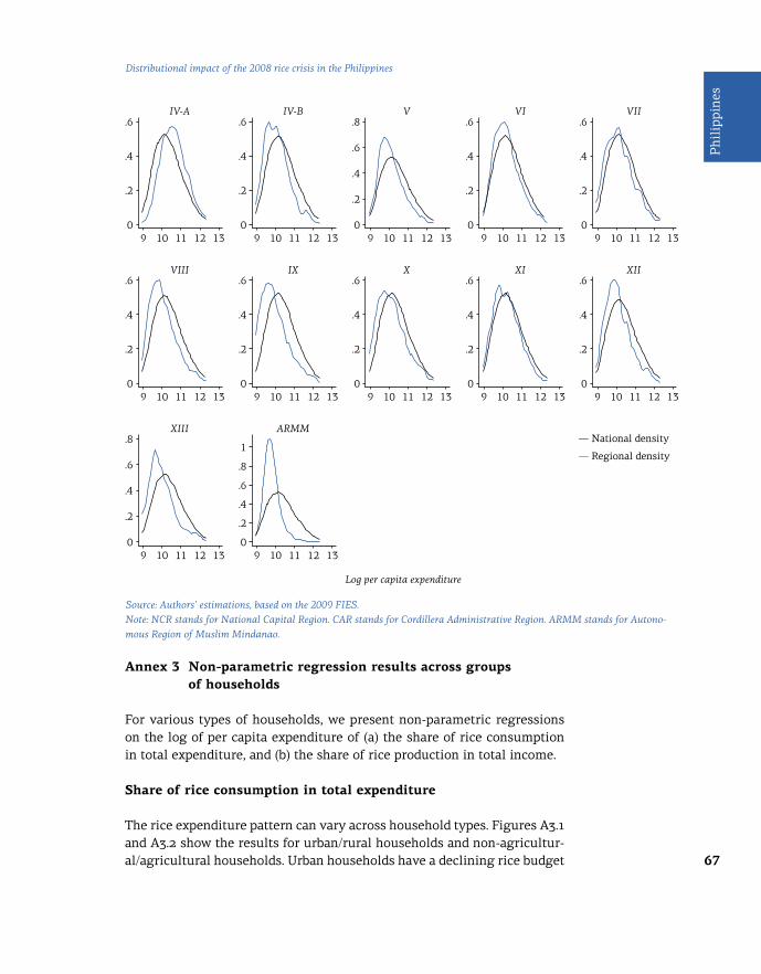
67
Phi
lipp
ines
Distributional impact of the 2008 rice crisis in the Philippines
Source: Authors’ estimations, based on the 2009 FIES. Note: NCR stands for National Capital Region. CAR stands for Cordillera Administrative Region. ARMM stands for Autono-mous Region of Muslim Mindanao.
Annex 3 Non-parametric regression results across groups of households
For various types of households, we present non-parametric regressions on the log of per capita expenditure of (a) the share of rice consumption in total expenditure, and (b) the share of rice production in total income.
Share of rice consumption in total expenditure
The rice expenditure pattern can vary across household types. Figures A3.1 and A3.2 show the results for urban/rural households and non-agricultur-al/agricultural households. Urban households have a declining rice budget
IV-A.6
0
.2
.4
9 13121110
IV-B.6
0
.2
.4
9 13121110
V.8
.6
0
.2
.4
9 13121110
XIII.8
.6
0
.2
.4
9 13121110
VI.6
0
.2
.4
9 13121110
VII.6
0
.2
.4
9 13121110
VIII.6
0
.2
.4
9 13121110
IX.6
0
.2
.4
9 13121110
X.6
0
.2
.4
9 13121110
XI.6
0
.2
.4
9 13121110
XII.6
0
.2
.4
9 13121110
ARMM
1
.8
.6
0
.2
.4
9 13121110
Log per capita expenditure
― National density
― Regional density

68
Trade policies, household welfare and poverty alleviation
share across the spectrum. However, for rural and agricultural households, there is a slight hump for households with lower levels of expenditure. Rural or agricultural households at very low levels of expenditure are like-ly to increase the share of rice in their budget when their incomes rise. Since rice is a basic food item in a food basket of a typical household, it is reasonable to expect that the poorest rural or agricultural households would put a premium on rice over other expenditure items. However, with a significant increase in income, they would start spending more on oth-er non-rice items. In the plot line for rural and agricultural households in Figure A3.1, this insight is reflected in the downward portion of the hill.
Figure A3.1 Budget share of rice and per capita expenditure by level of urbanity
Source: Authors’ estimations, based on the 2009 FIES.
0
.1
.2
Bud
get
shar
e
Log per capita expenditure
.3
9 10 11 12
― Total
― Rural
Urban
13

69
Phi
lipp
ines
Distributional impact of the 2008 rice crisis in the Philippines
Source: Authors’ estimations, based on the 2009 FIES.
Figure A3.2 Budget share of rice and per capita expenditure by agricultural household indicator
Share of rice production in total income
The rice production pattern can also vary across types of households. For instance, Figure A3.3 shows that, in general, rural households have a high-er income share of rice. This suggests that relative to urban households, rural households earn more of their income from rice production. For ur-ban households, the share of rice in income is small, and as households become better off, it gets even smaller. In contrast, for rural households at low levels of expenditure, the share of rice in income tends to be relatively constant up to a given level of expenditure, and then it falls considerably.
0
.05
.1
.15
.2
Bud
get
shar
e
Log per capita expenditure
.25
9 10 11 12 13
― Total
― Agricultural
Non-agricultural

70
Trade policies, household welfare and poverty alleviation
Figure A3.3 Income share of rice and per capita expenditure by level of urbanity
Source: Authors’ estimations, based on the 2009 FIES.
The regression for non-agricultural households in Figure A3.4 indicates a small income share of rice and displays an almost flat trend. We can, how-ever, see a much more interesting result when we look at the result for agricultural households. Unsurprisingly, across all levels of expenditure, the rice income share is higher in agricultural households than in non-ag-ricultural households. While all of the regressions of rice income shares presented so far show a downward trend, the result for agricultural house-holds shows an irregular pattern: as the level of expenditure increases, the share of rice in the income of agricultural households rises, declines, and then rises again.
23 For the definition of the benefits/costs variable, refer to Section 6.2.
0
.02
.04
.06In
com
e sh
are
Log per capita expenditure
.08
9 10 11 12
― Total
― Rural
Urban
13

71
Phi
lipp
ines
Distributional impact of the 2008 rice crisis in the Philippines
Figure A4.1 Histograms of the benefits/costs variable by gender of household head
Source: Authors’ estimations, based on the 2009 FIES.
Source: Authors’ estimations, based on the 2009 FIES.Note: The vertical lines represent x = 0.
Figure A3.4 Income share of rice and per capita expenditure by agricultural household indicator
Annex 4 Histograms of the benefits/costs variable for various groups of households23
0
0 0
.05
.1
5
5
.15
10
10
Inco
me
shar
eD
ensi
ty
Den
sity
Log per capita expenditure
Average benefits/costs Average benefits/costs
Male Female
.2
15 20
15
9 10 11
-.0407118 -.0371914
12 13
― Total
― Agricultural
Non-agricultural

72
Trade policies, household welfare and poverty alleviation
Figure A4.2 Histograms of the benefits/costs variable by level of urbanity
Figure A4.3 Histograms of the benefits/costs variable by agricultural household indicator
Source: Authors’ estimations, based on the 2009 FIES.
Source: Authors’ estimations, based on the 2009 FIES.
0
0
0
0
25
52
4
6
10
104
Den
sity
Den
sity
Den
sity
Den
sity
Average benefits/costs
Average benefits/costs
Average benefits/costs
Average benefits/costs
Rural
Agricultural
Urban
Non-agricultural
1020
208
8 15
156
-.0440582
-.0360043
-.0358483
-.0411262

73
Phi
lipp
ines
Distributional impact of the 2008 rice crisis in the Philippines
Figure A4.4 Histograms of the benefits/costs variable by national income decile
Source: Authors’ estimations, based on the 2009 FIES.
Average benefits/costs
First decile
-.0545198
Den
sity
8
10
0
2
4
6
Den
sity
Average benefits/costs
Second decile
-.0566074D
ensi
ty
8
10
0
2
4
6
Average benefits/costs
Third decile
Den
sity
8
10
0-.0539122
Average benefits/costs
Fourth decile
Den
sity
0
15
10
5
-.0429883Average benefits/costs
Fifth decile
-.0460456
Den
sity
15
0
5
10
Average benefits/costs
Sixth decile
-.0392547D
ensi
ty 15
20
0
5
10
Average benefits/costs
Seventh decile
Den
sity
-.0322305
15
20
0
5
10
Average benefits/costs
Eighth decile
-.0275607
Den
sity
30
0
10
20
Average benefits/costs
Ninth decile
-.0215164
Den
sity
40
0
10
20
30
Average benefits/costs
Tenth decile
-.0135478
50
0
10
20
30
40

74
Trade policies, household welfare and poverty alleviation
References
Balatibat, J. and Nierras, P. (2005). “The Female Headship in the Philippines: A Poverty Analysis.” Undergraduate thesis, University of the Philippines, School of Economics.
Balisacan, M., Sombilla, M.A. and Dikitanan, R.C. (2010). “Rice Crisis in the Philippines: Why Did It Occur and What Are Its Policy Implications?” In: Dawe, D. Ed. Rice Crisis: Markets, Policies and Food Security. Rome, London and Washington DC: Food and Agriculture Organization of the United Nations and Earthscan.
Bernardino, N. (2011). “Implications of Female Household Headship on Consumption Expenditure for Children’s Welfare: Philippine Case.” Paper presented at the International Association for Feminist Economics Annual Conference. Zheijang Gongshang University, Hangzhou, 24–26 June. Available at: http://editorialexpress.com/conference/IAFFE2011/program/IAFFE2011.html#5.
Briones, R. (2012a). “Rice Self-Sufficiency: Is It Feasible?” PIDS Policy Note No. 2012-13 (September). Philippine Institute for Development Studies, Manila.
Briones, R. (2012b). “Policy Coordination for Food Security: The Case of the ASEAN Rice Trade Forum.” PIDS Policy Note No. 2012-13 (September). Philippine Institute for Development Studies, Manila.
Bureau of Agricultural Statistics (2013). 2006–2013 Country Statistics Philippines [online]. Available at: http://countrys-tat.bas.gov.ph/?cont=1.
Chant, S. (1997). “Women-headed Households: Poorest of the Poor? Perspectives from Mexico, Costa Rica and the Philippines.” IDS Bulletin, 28 (3): 26–48.
Chant S. (2006). Poverty Begins at Home? Questioning Some (Mis)conceptions about Children, Poverty and Privation in Female-headed Households. London: Routledge.
Chant, S. (2008). “Dangerous Equations? How Female-headed Households Became the Poorest of the Poor: Causes, Consequences and Cautions.” In: Momsen, J. Ed. Gender and Development: Critical Concepts in Development Studies. Vol. 1. London: Routledge.
Clarete, R. (2012). “Enhancing ASEAN’s Resiliency to Extreme Rice Price Volatility.” ADB Sustainable Development Working Paper No. 23. Asian Development Bank, Manila.
Dawe, D. and Slayton, T. (2010). “The World Rice Market Crisis of 2007–8.” In: Dawe, D. Ed. Rice Crisis: Markets, Policies and Food Security. Rome, London and Washington DC: Food and Agriculture Organization of the United Nations and Earthscan.
Deaton, A. (1989). “Rice Prices and Income Distribution in Thailand: A Non-Parametric Analysis.” Economic Journal, 99 (395): 1–37.
Despuez, O. (2013). “Government Rice Inventory Dips Below Minimum Required Amid Post-Disaster Relief.” Interaksyon [online], 9 December. Available at: http://www.interaksyon.com/business/76513/govt-rice-inventory-dips-below-minimum-required-amid-post-disaster-relief.
Fujii, T. (2013). “Impact of Food Inflation on Poverty in the Philippines.” Food Policy, 39 (C): 13–27.
Heady, D. and Fan, S. (2008). “Anatomy of a Crisis: The Causes and Consequences of Surging Food Prices.” IFPRI Discussion Paper No. 00831. International Food Policy Research Institute, Washington DC.
75
Phi
lipp
ines
Distributional impact of the 2008 rice crisis in the Philippines
Intal, P. Jr. (1994). The State of Poverty in the Philippines. Understanding Poverty and Inequity in the Philippines: A Compendium of Policy and Methodological Researches. National Economic and Development Authority and United Nations Development Programme, Manila.
IRRI (2013). Why Does the Philippines Import Rice? [online]. International Rice Research Institute, Manila. Available at: http://www.irri.org/news/hot-topics/why-does-the-philippines-import-rice.
Klasen S. and Wink, C. (2003). “Missing Women: Revisiting the Debate.” Feminist Economics, 9: 263–299.
Klasen, S., Lechtenfeld, T. and Povel, F. (2011). “What about the Women? Female Headship, Poverty and Vulnerability in Thailand and Vietnam.” Courant Research Centre Discussion Paper No. 76. Courant Research Centre, Göttingen.
Lampietti, J. and Salker, L. (2000). “Consumption Expenditure and Female Poverty: A Review of Evidence.” Policy Research Report on Gender and Development, Working Paper No. 11. World Bank, Washington DC.
Marcoux, A. (1998). “The Feminization of Poverty: Claims, Facts, and Data Needs.” Population and Development Review, 24 (1): 131–139.
NSCB (2013). Revised/Rebased Annual National Accounts (1998–2011) [online]. National Statistical Coordination Board. Available at: http://nscb.gov.ph/sna/DataCharts.asp.
Reyes, C.M., Sobrevinas, A.B., Bancolita J. and de Jesus, J. (2009). “Analysis of the Impact of Changes in the Prices of Rice and Fuel on Poverty in the Philippines.” Discussion Paper Series No. 2009-07. Philippine Institute for Development Studies, Manila.
Rosenhouse, S. (1994). “Identifying the Poor: Is Headship a Useful Concept?” Living Standards Measurement Study, Working Paper No. 58. World Bank, Washington DC.
Sarris, A. (2010). “Trade-related Policies to Ensure Food (Rice) Security in Asia.” In: Dawe, D. Ed. Rice Crisis: Markets, Policies and Food Security. Rome, London and Washington DC: Food and Agriculture Organization of the United Nations and Earthscan.
Schelzig, K. (2005). Poverty in the Philippines: Income, Assets and Access. Asian Development Bank, Manila.
Timmer, C.P. (2010). “Did Speculation Affect World Rice Prices?” In: Dawe, D. Ed. Rice Crisis: Markets, Policies and Food Security. Rome, London and Washington DC: Food and Agriculture Organization of the United Nations and Earthscan.
Timmer, C.P. and Dawe, D. (2010). “Food Crises Past, Present (and Future?): Will We Ever Learn?” In: Dawe, D. Ed. Rice Crisis: Markets, Policies and Food Security. Rome, London and Washington DC: Food and Agriculture Organization of the United Nations and Earthscan.
UNCTAD (2011). Who is benefitting from trade liberalization in Cape Verde: A Gender Perspective. United Nations publication. UNCTAD/OSG/2011/2. New York and Geneva.
UNESCAP (2010). Women in Poverty in the Philippines: A Review of Extant Studies, Policies, and Programmes and Survey Report. United Nations Economic and Social Commission for Asia and the Pacific, Bangkok.
USDA (2013). Rice Yearbook 2013. United States Department of Agriculture, Foreign Agricultural Service, Washington DC.
World Bank (2001). Engendering Development: Through Gender Equality in Rights, Resources, and Voice. World Bank Policy Research Report. Washington DC and New York: World Bank and Oxford University Press.

76
Trade policies, household welfare and poverty alleviationFormer Yugoslav Republic of Macedonia

77
FYR
OM
Increasing the welfare effect of the agricultural subsidy programme for food crop production in the former Yugoslav Republic of Macedonia
Abstract
The objective of this study is to analyse the welfare implications of increas-ing prices of wheat, maize and rice, and agricultural subsidies on house-hold welfare in the former Yugoslav Republic of Macedonia. Based on this analysis, we propose a redesign of the subsidy programme for these crops, which might help to improve the welfare of households. The results sug-gest that the effects of increased commodity prices and the current subsi-dy programme were positive only for male-headed rural households. The newly proposed disbursement scheme for government subsidies is there-fore based on targeting female-headed rural households for both wheat and rice, all poor urban households for wheat, and male-headed rural households for rice. Results of the simulation with regard to wheat-maize production suggest that targeting poor urban households could result in a significant welfare effect ranging up to 30–40 per cent of the income of this group of households, assuming it is accompanied by a usufruct of state-owned land and start-off grants for initial investment. Targeting poor female-headed rural households may increase the impact of the scheme from almost zero to about two-thirds of the income of poor male-head-ed rural households. The effect on the welfare of poor rural rice produc-ers may also be large – up to 20 per cent of household income – taking into account that a considerable effort is however needed to start off rice production.
* The author would like to thank Nikica Mojsoska Blazevski, Adviser to the Ministry of Labour and Social Policy, Margarita Deleva from the Ministry of Agriculture, and Biljana Trajkovska from the Ministry of Labour and Social Policy of the former Yugoslav Republic of Macedonia for their support in the preparation of this study.
Marjan Petreski *
78
Trade policies, household welfare and poverty alleviation
1 Introduction
Food crop commodities – namely wheat, maize and rice – are important in the former Yugoslav Republic of Macedonia: 24.5 per cent of house-holds farm one or more of these crops, and more than 50 per cent of ru-ral households spend more than 10 per cent of their budget on them. The overall poverty rate, based on the relative poverty line,1 was estimated at 27.1 per cent in 2011 – up from 25 per cent in 2006 – while rural poverty was at 37.6 per cent in 2011. Given that more than a fourth of the popula-tion lives below the poverty line, it is not a coincidence that a large por-tion of poor household income is spent on food crop commodities and the derived products.
Prices of food crop commodities have been rising since 2006: in October 2012, they were 46.5 per cent higher than the average level in 2006. The in-crease has been widespread, but the aforementioned commodities – wheat (118 per cent), maize (165 per cent), and rice (76 per cent) – have experi-enced price increases larger than other commodities over the same period. However, the production of food commodities has been declining since the 1990s when the planning system was abandoned; at present, it is on aver-age 60 per cent of the production in 1991, though the level varies across the different crops. The increase in prices has been insufficient to increase the production.
Commodity price developments may have large impacts on real incomes of poor households in developing countries. However, little information is available on actual impacts on the poor, despite some concerns expressed in the literature (e.g. FAO, 2011; World Bank, 2008). The overall impact of commodity price increases on the welfare of the poor depends on wheth-er the gains to poor producers outweigh the adverse impacts on poor con-sumers, on the pattern and response of household income, and on the policy responses. It has been widely claimed that the effects are quite di-verse and country-specific (Hertel and Winters, 2006).
Agricultural subsidies have been among government policy programmes generally pursued in times of commodity price increases (Wodon and Zaman, 2010). The right-oriented government of the former Yugoslav Republic of Macedonia, which took office in late 2006, undertook an am-bitious agenda for subsidizing agriculture with budget funds that reached 4.5 per cent of total government expenditure in 2011 from virtually zero in 2006. Despite ambiguously communicated, it seems that an overarching
1 The relative poverty line is 60 per cent of the median equivalent income.

79
FYR
OM
Increasing the welfare effect of the agricultural subsidy programme for food crop production in the FYROM
objective of the programme was to increase production and improve the living conditions of those who are predominantly living or temporarily migrating to rural areas. The programme was designed so that any produc-tion would be subsidized with specifically determined lump sums, to sup-port current producers as well as steer former producers to resume crop production. The food crop commodities mentioned above have been subsi-dized as follows: EUR 150 per cultivated hectare (ha) up to 10 ha of cultivat-ed land; EUR 90 per ha for 10–50 ha; EUR 45 per ha for 50–100 ha; and EUR 15 per ha for more than 100 ha. No special conditions regarding the type of household producing staple foods applied to benefit from the programme.
However, the effects of the agricultural subsidy programme have been, to a large extent, unsatisfactory. Despite an increase in government subsidies, the production of all food crop commodities – except for rice – has further declined, while household welfare – judging by the increase in poverty – has not improved.
Two related policy questions therefore arise. First, what are the likely ef-fects of the observed change in the level of food crop prices on household welfare in the former Yugoslav Republic of Macedonia? Second, what are the likely effects of the government subsidy programme on household welfare, and could another subsidy disbursement scheme strengthen the impact on the welfare of households? This study provides an analytical background for discussion of these questions.
Ideally, our analysis would use household surveys undertaken before and after the price increases and the introduction of the government subsidy programme. This would allow a precise analysis of the effects of the price change and the subsidy on the welfare of households and on farm sup-ply behaviour. However, such data do not exist – or at least not entirely. Instead we therefore use the 2011 Household Budget Survey (HBS), which however does not provide any information on subsidies. Hence, we apply the rules for subsidy disbursement specified above to evaluate their effect. Based on the findings, we propose another scheme for disbursement (for the three crops analysed here) that aims to improve the welfare of house-holds in the former Yugoslav Republic of Macedonia. Therefore, the fo-cus of the study is on the welfare implications of the price increases and government subsidies. We first evaluate how household welfare was af-fected by the increasing prices of the most important crops, and second, how it was affected by the subsidies which the government introduced for crop farming. Subsequently, we present a new agricultural subsidy pro-gramme for food crops redesigned into a tool to alleviate (rural) poverty in the country.
80
Trade policies, household welfare and poverty alleviation
No in-depth analysis has been undertaken thus far to help understand the consumption and income patterns of households in the former Yugoslav Republic of Macedonia and their decisions with regard to cultivating crop commodities. In particular, the effect of government subsidies remains fully unexamined. Many economists and former policymakers in the for-mer Yugoslav Republic of Macedonia argue that the design of the govern-ment agricultural subsidy programme is arbitrary and uninformed, and hence does not act as a mechanism for maximizing the poverty-reduction effect. The design of the programme thus continues to be a topic of heat-ed public debate. The study is organized as follows: Section 2 presents the HBS data and ex-plains how they meet the particular needs of the analysis. It also explores some of the distinguishing features of household income that anticipate the more sophisticated estimation results that follow. Section 3 gives a brief overview of the relevant literature and sets this study’s place in the literature. Section 4 outlines the analytical framework, which is the one applied in Deaton (1989a, 1989b). Section 5 charts the distributional re-sults of a change in crop prices and the introduction of government subsi-dies, and proposes a new disbursement scheme that improves the impact on welfare. The conclusions are presented in Section 6.
2 Stylized facts
2.1 Macroeconomic aspects
Despite being a poor republic in the former Yugoslavia, the former Yugoslav Republic of Macedonia had a larger production of food crops in 1992 than nowadays. Figure 1 shows the production patterns of the three food crops analysed here, namely wheat, maize and rice. The general non-increas-ing trend of production is evident for all three crops, with largely empha-sized volatility. The introduction of government subsidies in 2007 did not change these patterns – at least not as expected: only rice production in-creased, but as a continuation of an increasing trend that had begun ear-lier, while the production of the other two crops stagnated or declined. In addition, as Figure 2 suggests, the share of imported cereals in total con-sumption increased.

81
FYR
OM
Increasing the welfare effect of the agricultural subsidy programme for food crop production in the FYROM
Figure 1 Production of food crop commodities, 1992–2010 (thousands of metric tons)
Figure 2 Production versus import of cereals, 1998–2012 (per cent)
Source: Author’s calculations, based on FAO statistics and State Statistical Office.Note: LHS stands for left-hand scale, RHS for right-hand scale.
Source: Author’s calculations, based on FAO statistics and National Bank of the Republic of Macedonia.
Figure 3 presents the price changes that accompanied these production patterns. At the same time that the government subsidy programme was introduced, food commodities marked the largest price increase in years, mainly due to weather-related shortages occurring in different countries worldwide. The increase in prices was widespread, but the food crops ana-lysed here experienced the largest price increases between 2006 and 2012 at the international stage: wheat (118 per cent), maize (165 per cent), and rice (76 per cent).
1992
450 45
400 40
350 35
300 30
250 25
200 20
150 15
100 10
50 5
1993
1994
1995
1996
1997
1998
1998
100
90
80
70
60
50
40
30
20
10
0
1999
1999
2000
2000
2001
2001
2002
2002
2003
2003
2004
2004
2005
2005
2006
2006
2007
2007
2008
2008
2009
2009
2010
2010
2011
2011
2012
― Wheat (LHS)
― Maize (LHS)
Rice (RHS)
Tho
usan
ds o
f m
etri
c to
ns
Subsidies
Tho
usan
ds o
f m
etri
c to
nsPe
r ce
nt
■ Production □ Imports

82
Trade policies, household welfare and poverty alleviation
Figure 3 Prices of food commodities, 2000–2012 (USD per metric ton)
Table 1 Structure of the survey
Source: Author’s calculations, based on IMF statistics.
Source: 2011 HBS.
2.2 Microeconomic patterns of demand and supply
We use data from the 2011 HBS2 to describe the patterns of demand and supply of wheat, maize and rice, with respect to urban/rural households and gender of the household head. Table 1 shows the number of surveyed households and their distribution over the country. A total of 3,566 sur-veyed households are analysed; these households are distributed over two geographical sections and by gender of household head. Although the share of urban households may be overrepresented, due to a lower expense in surveying urban households, in this study we will use the weights ob-tained alongside the dataset to correct for this issue.
Geographical distribution
Urban Rural Total
Gender of head of household
Male 2,092 817 2,909
Female 553 104 657
Total 2,645 921 3,566
2 Ideally, we would have preferred to start with the 2006 HBS (the survey before the price hike), but data on the income and expenditure of cereals (wheat and maize) and rice were largely missing because surveyed households at that time were answering the survey on a voluntary basis only. However, the 2011 HBS served the purpose well, because, as observed in Figure 1, no large changes in the produced quantities occurred between 2006 and 2011.
1200
1000
800
600
400
200
0
2000
2001
2002
2003
2004
2005
2006
2007
2008
2009
2010
2011
2012
― Wheat
― Maize
Rice
U
SD p
er m
etri
c to
n

83
FYR
OM
Increasing the welfare effect of the agricultural subsidy programme for food crop production in the FYROM
Table 2 Summary statistics
Table 2 presents sample means for the main variables of interest. Throughout this study, we will be using total household income per capita as a preferred measure of household living standards. Judging by this crite-rion, and ignoring any price differences, households in urban areas have a higher living standard than those in rural areas, and female-headed house-holds are wealthier than male-headed households. While the first regulari-ty is expected, the second regularity may be surprising, but still logical for the former Yugoslav Republic of Macedonia – at least partially. Namely, in a predominantly still patriarchic-minded society, a female-headed house-hold signifies that a male head has passed away or migrated; in the former case, this reduces the household size (as well as total income); in the lat-ter case, with the reduction of its size, the household is likely to receive re-mittances, which elevate its per capita income.3 It could be observed that the average household size is lower for female-headed households, where-as the difference in household size between urban and rural households is likely insignificant. Finally, the average age of the head of household is quite high, due to households often consisting of grandparents, parents and children, with a grandparent reported as head of household.
All HHGeographical distribution
Gender of head of household
Urban Rural Male Female
HH characteristics
HH sizeAge of HH headIncome per capita
3.855.7
6,125
3.755.4
6,928
4.156.9
3,744
4.053.9
5,778
2.862.6
7,470
Annual production (kg per HH)
Wheat/maizeRice
886.137.7
0.30
3,511.7149.5
955.745.5
616.910.8
Annual expenditure (kg per HH)
Wheat/maizeRice
293.727.3
136.527.7
759.726.0
304.727.3
251.127.0
Annual self-consumption (kg per HH)
Wheat/maizeRice
14.80.2
00
58.80.7
15.90.2
10.80.02
Income share(per cent)
Wheat/maizeRice
5.20.3
00
20.71.2
5.60.3
3.80.3
3 Remittances are an important source of income in the former Yugoslav Republic of Macedonia, amounting to more than 4 per cent of GDP per year. About one-fourth of the households are remittance receivers.

84
Trade policies, household welfare and poverty alleviation
Source: Author’s calculations, based on the 2011 HBS.Note: HH stands for household, kg for kilogram; income per capita is measured in Macedonian denar (MKD).
All HHGeographical distribution
Gender of head of household
Urban Rural Male Female
Expenditure share (per cent)
Wheat/maizeRice
1.70.6
0.80.6
4.30.6
1.70.6
1.80.7
Self-consumption share (per cent)
Wheat/maizeRice
0.10
00
0.40
0.10
0.10
The fourth and fifth columns of Table 2 show the geographical and gender distribution of crop quantities, and income and expenditure shares. At the outset, it is estimated that in the former Yugoslav Republic of Macedonia, about 90,000 households cultivate wheat and maize, and about 10,000 to 11,000 cultivate rice. Expectedly, urban households do not produce these crops (or they do so in a negligible amount); hence we will focus on rural households. Wheat and maize appear to be an important source of income for rural households – a rural household produces on average 3.5 metric tons of wheat and maize per year and earns about 21 per cent of its income from cultivation. About one-fifth of that amount is the average expendi-ture on wheat and maize per rural household, which is five times more than for urban households. Note that under expenditure on wheat and maize, we count both grains and bread produced, given an aggregation of household expenditures in the household survey. The figures nevertheless seem plausible because the share of bread in the consumption basket of rural households is higher due to rural households being poorer than ur-ban households and to their continued tradition to bake bread domestically. Female-headed households produce one-third less wheat and maize than male-headed households, which underscores the role played by males in cultivating this crop (including the necessity to handle large machinery).
The importance of rice in both income and consumption of households in the former Yugoslav Republic of Macedonia is significantly lower than for wheat and maize. Rice is also almost exclusively produced in rural house-holds: male-headed households are larger producers in absolute terms, but rice production has equal importance, in relative terms, for both male- and female-headed households. Likewise, both types of households are not dif-ferent in their consumption of rice.
Nevertheless, the averages presented in Table 2 are likely insufficient to consider the distributional effects of potential price changes on the crops considered here. There are rich and poor households in both rural and ur-ban regions and across male- and female-headed households. Production

85
FYR
OM
Increasing the welfare effect of the agricultural subsidy programme for food crop production in the FYROM
and consumption patterns are far from being independent of household re-sources. If it is true that wealthier households are those that produce crops for sale, while poor households hardly satisfy their own needs, then the di-rect effects of higher prices, while being potentially beneficial for the en-tire sector (especially the rural one), might as well worsen the income of poor households. Figures 4 and 5 show the estimates of the distribution of living standards across households by both geographical section and gen-der. The kernel-smoothing graphs illustrate the estimated density func-tions of the logarithm of household per capita income.4
4 We use the logarithm of the income per capita, as it is usually strongly positively skewed.
Figure 4 Per capita income distribution by geographical section
Figure 5 Per capita income distribution by gender of household head
Source: Author’s estimations, based on the 2011 HBS.
Source: Author’s estimations, based on the 2011 HBS.
.6
.8
.6
.4
.4
.2
.2
0
0
8
8
9
9
10
10
11
11
12
12
13
13
Den
sity
Den
sity
Log per capita income
Log per capita income
― All
– – Rural
Urban
― All
– – Male
Female
86
Trade policies, household welfare and poverty alleviation
The figures show a difference between the wealth of urban and rural house-holds, in favour of the former; although the difference may seem small, it is still important given the logarithmic scale. However, rural households in the middle of the distribution are wealthier than their urban counter-parts and then extend into a long upper tail, suggesting that there are very rich households even within the rural sector. Conversely, the contin-gent of wealthy urban households is quite pronounced. Figure 5 suggests that female-headed households are more “equal” in terms of income than male-headed households. Male-headed households are more likely to be observed in both the poor and the rich tails of the income distribution.
Considering (a) the importance of wheat and maize for households in the former Yugoslav Republic of Macedonia, (b) the price spike since 2006, (c) the implementation of government subsidies, and (d) the diversity of households in terms of wealth, the discussion above highlights the impor-tance of evaluating the effects of increasing prices and agricultural sub-sidies on the welfare of households. This will be the aim of our analysis.
3 Literature review
Recent spikes in global food prices have sparked a new strand of literature to investigate their effects on poverty. For instance, using household level information for selected low-income countries, Ivanic and Martin (2008) find that the share of the population living below the poverty line has in-creased as a result of higher food prices in eight of the nine countries in-cluded in their study. Similarly, de Hoyos and Medvedev (2011) provide a formal assessment of the implications of higher prices for global pover-ty using a representative sample of 63 to 93 per cent of the population of the developing world. Their study finds an increase in extreme poverty5 headcount at the global level of 1.7 percentage points, albeit ranging from negligible in Eastern Europe to considerably large in sub-Saharan Africa. A similar magnitude of poverty increase due to price hikes is found by Wodon et al. (2008) in sub-Saharan Africa.
An also recent study by Aksoy and Isik-Dikmelik (2008) however challeng-es the idea that higher food prices unambiguously deteriorate the income of the poor. Using household survey data from nine low-income countries, the study finds that net sellers are disproportionately represented among
5 Extreme poverty refers to a condition that is characterized by severe deprivation of basic human needs, including food, safe drinking water, sanitation facilities, health, shelter, education and information. It depends not only on income but also on access to services.
87
FYR
OM
Increasing the welfare effect of the agricultural subsidy programme for food crop production in the FYROM
the poor, hence an increase in food prices could transfer income from rich-er to poorer households. However, many other studies (e.g. Poulton et al., 2006; Christiaensen and Demery, 2007) argue that the rural poor are more frequently net buyers and thus a price increase exerts a negative impact on them. Consequently, although studies tend to find that higher food prices have a negative impact on the poor, the relationship is neither unique nor universal, but depends on the specific context (Hertel and Winters, 2006). Earlier studies (e.g. Deaton, 1989a; Ravallion, 1990; Ravallion and van de Walle, 1991; Friedman and Levinsohn, 2002), other than offering contribu-tion to the methodological approach to this issue, examine similar issues and provide specific policy recommendations for specific countries.
In contrast to this discussion, the effect of agricultural subsidies – as a po-tentially countervailing programme to rising food prices6 – on household welfare and poverty remains largely unexamined. Only Wodon and Zaman (2010) discuss agricultural subsidies as a policy to counter the effects of rising food prices, but no estimates have been provided in this context. The present study therefore builds on these grounds. It will estimate the welfare effect of changes in crop prices and propose a redesign of govern-ment subsidies to improve their effect on alleviating poverty in the former Yugoslav Republic of Macedonia.
4 Methodology and data
4.1 Methodology
The analysis of the distributional impact of price increases follows a meth-odology outlined by Singh et al. (1986) and Deaton (1989a, 1997), and sub-sequently widely applied (Barrett and Dorosh, 1996; Budd, 1993; Ivanic and Martin, 2008; Wodon et al., 2008; Klytchnikova and Diop, 2010). The argu-ment made is that the non-parametric techniques in Deaton’s methodol-ogy do not impose any structure on the data and hence make full use of the information available. Deaton’s framework can be summarized as fol-lows. The change in welfare following a change in prices for a household is:
6 We should note here that for a country that imports food and is a price taker on world markets, such as the former Yugoslav Republic of Macedonia, a consumption subsidy would countervail increasing food prices by lowering the domestic price of consumed food. However, a production subsidy – the one analysed here – would further increase domestic food prices. Therefore, interpretation of our findings should be made with caution from this viewpoint.

88
Trade policies, household welfare and poverty alleviation
∆wi j = ∑j=1
∆pj [( prodij – consij ) + ηjLi ] (1)
where ∆wij is the welfare effect expressed in percentage terms of the initial consumption level of household i for good j, ∆pj is the percentage change in prices for each good considered (category by category), prodij is the in-come share coming from production of good j (household sales of item j divided by total income), consij is the expenditure share of good j (house-hold consumption of item j divided by total consumption), ηj is the wage rate elasticity with respect to changes in prices of good j, and Li is the la-bour share in household income.
Our analysis proceeds as follows. We use non-parametric techniques to estimate the production, consumption and labour income effects of the observed price changes over 2006–2012. We disentangle the effects on households by geographical distribution and gender to be able to judge which target group, which part of the income distribution and which spe-cific food crop commodity may benefit the most from agricultural subsidies.
Once we identify these groups, we conduct a simulation of the effect of subsidies using equation (1). Based on the findings, we propose a scheme for disbursement of the proposed amount of agricultural subsidies for 2012, i.e. we direct the funds to specific groups of households instead of them being disbursed linearly to everyone. We then evaluate the welfare effects of this alternative subsidy scheme.
To undertake the analysis, we need information on household production, consumption and sales of the above agricultural products. For conduct-ing the proposed research, the Household Budget Survey of the former Yugoslav Republic of Macedonia in 2011 is used. In addition to the usu-al demographic and labour market data, the HBS contains data on produc-tion and consumption of the above-mentioned food crops. A disadvantage, however, is that the HBS reports those parameters for wheat and maize grains together. With rice, this gives two categories of food commodities to be analysed in this study.
4.2 Simulation
The HBS does not contain data for subsidies. We therefore analyse the im-pact of the existing scheme by applying the prevailing rules for subsidy disbursement. To evaluate the current scheme, which is based on lump sums per cultivated hectare and not per produced kilogram, we need to as-sume a certain production of the food crop per hectare. For this, we will use the average kilogram per hectare ratio for cereals of 3,373 metric tons
n

89
FYR
OM
Increasing the welfare effect of the agricultural subsidy programme for food crop production in the FYROM
Subsidy rules per hectare Subsidy rules per kilogram
EUR 150 per ha up to 10 ha 4.45 cents per kg up to 10 ha
EUR 90 per ha for 10–50 ha 2.67 cents per kg for 10–50 ha
EUR 45 per ha for 50–100 ha 1.33 cents per kg for 50–100 ha
EUR 15 per ha for above 100 ha 0.44 cents per kg for above 100 ha
Table 3 Conversion rates for crop subsidies, averages for 2006–2009
Source: Author’s calculations, based on Ministry of Agriculture, Forestry and Water Management.Note: The conversion follows these steps: First, we observe kilograms produced by a household; second, we use the conversion of 3,373 metric tons per hectare to find the plot size that a household owns; and third, based on this information, we compute the subsidy a household receives.
per hectare in the former Yugoslav Republic of Macedonia obtained from the Ministry of Agriculture, Forestry and Water Management. We will then base the simulation on the transformation of kilograms into hectares.
The simulation should make some assumptions with respect to the change in production due to subsidies. However, we should be cautious in this re-gard, as the stylized facts of Section 2 suggest that despite both price in-creases and government subsidies, crop production in the former Yugoslav Republic of Macedonia stagnated or continued to fall. As further support to this claim, Table 4 presents simple tests for structural breaks in the annual time series (1992–2012) for the nationwide quantity produced of wheat, maize and rice. If the subsidy had a bearing on production, one would expect to detect a structural shift after the implementation of the subsidy programme. The figures shown are the t-statistics for the signifi-cance of the potential shift in production when subsidies were introduced.7 The test does not claim that the potential shift has happened due to the introduction of subsidies only, but simply tests whether a shift has oc-curred. We consider three different years to capture lagged effects of the 2006 subsidy programme on production. Results suggest that a structur-al shift in the production cannot be claimed, as all t-statistics are within the “insignificance” range of between –1.96 and 1.96 for the 5 per cent sig-nificance level.
7 In essence, we regress the production on a constant term and a dummy variable for a shift in any of the three years (2006, 2007 and 2008).

90
Trade policies, household welfare and poverty alleviation
Table 4 Testing for structural breaks in production around the introduction of subsidies
Table 5 Reaction of production to subsidies
t-statistics
Wheat Maize Rice
2006 –0.6958 –0.0343 0.1502
2007 –1.3325 –1.4196 0.1532
2008 1.3015 0.4073 0.0855
Source: Author’s estimations, based on FAO statistics.
Source: Author’s estimations.Note: None of the estimated parameters are found to be significant at the 10 per cent level. § means that two lags of the independent variables are used as instruments.
Table 5 investigates the issue further. It portrays a simple regression of total cereal production on subsidies to check the magnitude with which they potentially affect production. The regression also includes prices, as these are expected to drag production up, and the log of income, so as to capture any general economic trends that may affect production (such as the ongoing crisis). We use annual time-series data over 2003–2012 collected from FAO statistics, the Ministry of Agriculture, Forestry and Water Management, and the State Statistical Office. We present results from an ordinary least squares (OLS) estimator, as well as from a general-ized method of moments (GMM) estimator, which take into account poten-tial endogeneity of variables (for instance, subsidies may lead to increased production, but more production will trigger a larger amount of subsidies to be paid out). However, all coefficients are insignificant, suggesting that in the case of the former Yugoslav Republic of Macedonia, subsidies (not increasing prices) are not correlated with increased production, which is fully in line with what we observe in Figure 1.
OLS GMM§
Log of income 1.18 1.34
Log of subsidies –0.24 –0.24
Prices –0.24 –0.53
Constant 0.59 –
For the analysis, we also need data on wages and total income of house-holds. The HBS provides data on all sources of income in households, so the share of labour income in the total income is readily available. The price pass-through and the wage-price elasticity with respect to prices are obtained as follows.
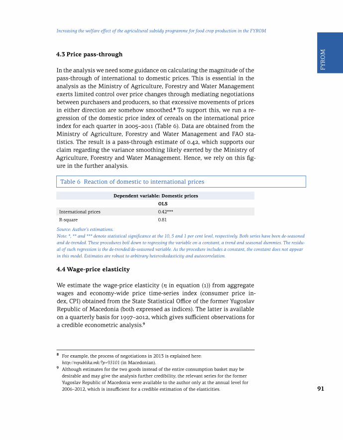
91
FYR
OM
Increasing the welfare effect of the agricultural subsidy programme for food crop production in the FYROM
Table 6 Reaction of domestic to international prices
Source: Author’s estimations. Note: *, ** and *** denote statistical significance at the 10, 5 and 1 per cent level, respectively. Both series have been de-seasoned and de-trended. These procedures boil down to regressing the variable on a constant, a trend and seasonal dummies. The residu-al of such regression is the de-trended/de-seasoned variable. As the procedure includes a constant, the constant does not appear in this model. Estimates are robust to arbitrary heteroskedasticity and autocorrelation.
4.3 Price pass-through
In the analysis we need some guidance on calculating the magnitude of the pass-through of international to domestic prices. This is essential in the analysis as the Ministry of Agriculture, Forestry and Water Management exerts limited control over price changes through mediating negotiations between purchasers and producers, so that excessive movements of prices in either direction are somehow smoothed.8 To support this, we run a re-gression of the domestic price index of cereals on the international price index for each quarter in 2005–2011 (Table 6). Data are obtained from the Ministry of Agriculture, Forestry and Water Management and FAO sta-tistics. The result is a pass-through estimate of 0.42, which supports our claim regarding the variance smoothing likely exerted by the Ministry of Agriculture, Forestry and Water Management. Hence, we rely on this fig-ure in the further analysis.
8 For example, the process of negotiations in 2013 is explained here: http://republika.mk/?p=93101 (in Macedonian). 9 Although estimates for the two goods instead of the entire consumption basket may be desirable and may give the analysis further credibility, the relevant series for the former Yugoslav Republic of Macedonia were available to the author only at the annual level for 2006–2012, which is insufficient for a credible estimation of the elasticities.
Dependent variable: Domestic prices
OLS
International prices 0.42***
R-square 0.81
4.4 Wage-price elasticity
We estimate the wage-price elasticity (η in equation (1)) from aggregate wages and economy-wide price time-series index (consumer price in-dex, CPI) obtained from the State Statistical Office of the former Yugoslav Republic of Macedonia (both expressed as indices). The latter is available on a quarterly basis for 1997–2012, which gives sufficient observations for a credible econometric analysis.9
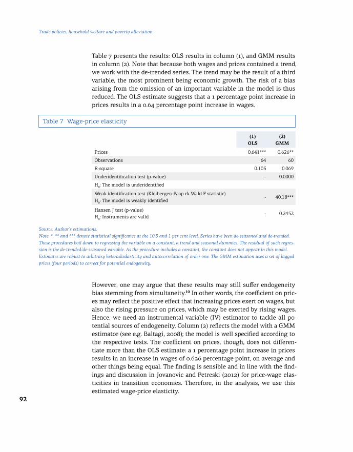
92
Trade policies, household welfare and poverty alleviation
Table 7 presents the results: OLS results in column (1), and GMM results in column (2). Note that because both wages and prices contained a trend, we work with the de-trended series. The trend may be the result of a third variable, the most prominent being economic growth. The risk of a bias arising from the omission of an important variable in the model is thus reduced. The OLS estimate suggests that a 1 percentage point increase in prices results in a 0.64 percentage point increase in wages.
Table 7 Wage-price elasticity
Source: Author’s estimations.Note: *, ** and *** denote statistical significance at the 10.5 and 1 per cent level. Series have been de-seasoned and de-trended. These procedures boil down to regressing the variable on a constant, a trend and seasonal dummies. The residual of such regres-sion is the de-trended/de-seasoned variable. As the procedure includes a constant, the constant does not appear in this model. Estimates are robust to arbitrary heteroskedasticity and autocorrelation of order one. The GMM estimation uses a set of lagged prices (four periods) to correct for potential endogeneity.
(1)OLS
(2)GMM
Prices 0.641*** 0.626**
Observations 64 60
R-square 0.105 0.069
Underidentification test (p-value) - 0.0000
H0: The model is underidentified
Weak identification test (Kleibergen-Paap rk Wald F statistic)H0: The model is weakly identified
- 40.18***
Hansen J test (p-value)H0: Instruments are valid
- 0.2452
However, one may argue that these results may still suffer endogeneity bias stemming from simultaneity.10 In other words, the coefficient on pric-es may reflect the positive effect that increasing prices exert on wages, but also the rising pressure on prices, which may be exerted by rising wages. Hence, we need an instrumental-variable (IV) estimator to tackle all po-tential sources of endogeneity. Column (2) reflects the model with a GMM estimator (see e.g. Baltagi, 2008); the model is well specified according to the respective tests. The coefficient on prices, though, does not differen-tiate more than the OLS estimate: a 1 percentage point increase in prices results in an increase in wages of 0.626 percentage point, on average and other things being equal. The finding is sensible and in line with the find-ings and discussion in Jovanovic and Petreski (2012) for price-wage elas-ticities in transition economies. Therefore, in the analysis, we use this estimated wage-price elasticity.

93
FYR
OM
Increasing the welfare effect of the agricultural subsidy programme for food crop production in the FYROM
10 Endogeneity bias may arise because of an omitted variable, measurement error and simultaneity. See further explanations in Wooldridge (2002). OLS estimates in this study have the omitted variable bias to an extent reduced by using de-trended series. However, the overall endogeneity may be addressed only by an IV estimator as is GMM.
5 Findings and discussion
This section presents the results of the analysis. Results are analysed and discussed in the following order: First, we present the welfare effects of the rising prices of wheat, maize and rice; second, we show the welfare ef-fects of government subsidies for these crops; and third, we describe the welfare results of a new proposed scheme for subsidy disbursement, which potentially increases the overall welfare and shields the vulnerable groups of households. Note that the sections visualize only the overall result de-composed into rural/urban and male-/female-headed households; the par-ticular components of the welfare function are shown in Annexes 1 and 2.
5.1 Welfare effects of rising prices
The welfare change in terms of share of household income due to the ob-served price change of wheat and maize between 2006 and 2011 at each point of the income distribution is estimated and plotted in Figures 6, 7 and 8 – the first refers to all households, and the next two refer to urban and rural households, respectively. Note that the respective price chang-es over this period for wheat-maize and rice are 102.5 per cent and 81.8 per cent, not considering the international-domestic price pass-through. The price change results in a positive welfare change for all households over the income distribution. However, when disaggregated according to gen-der, results suggest that male-headed households are better off and poor female-headed households are worse off.
Figure 6 Welfare change for all households due to increasing prices – Wheat and maize
Source: Author’s estimations, based on the 2011 HBS.
.04
.02
0
–.02
–.04
8 9 10 11 12 13
Wel
fare
cha
nge
Log per capita income
― All
– – Male head
Female head

94
Trade policies, household welfare and poverty alleviation
However, a more detailed look is worth considering. The disaggregation between urban and rural households is essential, because as we have seen in Section 2, urban households in the former Yugoslav Republic of Macedonia do not produce wheat and maize or do so negligibly. The re-sult is expectedly an overall negative welfare effect of increasing prices on those households – the effect being more pronounced on female-head-ed urban households (Figure 7). In contrast, the overall welfare effect on rural households is positive (Figure 8) – the effect being negative only on female-headed rural households in the negligible fourth percentile of the income distribution.
Figure 7 Welfare change for urban households due to increasing prices – Wheat and maize
Figure 8 Welfare change for rural households due to increasing prices – Wheat and maize
Source: Author’s estimations, based on the 2011 HBS.
Source: Author’s estimations, based on the 2011 HBS.
0
.8
–.01
.6
–.02
.2
.4
–.03
0
8
8
9
9
10
10
11
11
12
12
13
Wel
fare
cha
nge
Wel
fare
cha
nge
Log per capita income
Log per capita income
― All
– – Male head
Female head
― All
– – Male head
Female head

95
FYR
OM
Increasing the welfare effect of the agricultural subsidy programme for food crop production in the FYROM
Figure 9 Welfare change for all households due to increasing prices – Rice
Source: Author’s estimations, based on the 2011 HBS.
A closer look at the drivers of these results in Annex 1 suggests the usual Engel’s Law, or its wheat-maize equivalent – that, on average, the share of budget spent on wheat and maize declines as the living standard rises. It is also clear that female-headed households spend more on wheat-maize in the left part of the income distribution. However, while urban house-holds have virtually no income from wheat-maize (no production), rural households earn part of their income from this type of agricultural pro-duction, the share being larger for the poorer male-headed households. Female-headed poor households, interestingly, have a low income share from wheat-maize, which is likely due to the task of cultivating wheat and maize being perceived as a male job (due to the difficulty of cultivation and the necessity to handle large machinery). This fact then drives the nega-tive welfare effect of the price change on poor female-headed rural house-holds. It is worth mentioning that the labour income share in total budget increases with the level of income of the household but it occurs at a fast-er pace for urban households.
The welfare change in terms of share of household income due to the ob-served price change of rice between 2006 and 2011 at each point of the in-come distribution is estimated and plotted in Figures 9, 10 and 11 – the first refers to all households, and the next two refer to urban and rural house-holds, respectively. The price change results in a negative welfare effect on all female-headed households over the income distribution and on poor male-headed households.
.005
0
–.005
–.01
–.015
8 9 10 11 12 13
Wel
fare
cha
nge
Log per capita income
― All
– – Male head
Female head

96
Trade policies, household welfare and poverty alleviation
A more detailed look suggests that urban households are negatively affect-ed by the price increase along the entire income distribution. This is expect-ed, given that they do not produce rice, or do so negligibly. The result for rural households is mixed. Overall, only the poorest male-headed house-holds are slightly negatively affected and a small part of female-headed households (only about 6 per cent) on the left of the income distribution also shows a negative welfare change.
Figure 10 Welfare change for urban households due to increasing prices – Rice
Figure 11 Welfare change for rural households due to increasing prices – Rice
Source: Author’s estimations, based on the 2011 HBS.
Source: Author’s estimations, based on the 2011 HBS.
0
–.01
–.005
–.015
–.02
8 9 10 11 12 13
Wel
fare
cha
nge
Log per capita income
.01
.005
–.005
0
–.01
8 9 10 11 12
Wel
fare
cha
nge
Log per capita income
― All
– – Male head
Female head
― All
– – Male head
Female head

97
FYR
OM
Increasing the welfare effect of the agricultural subsidy programme for food crop production in the FYROM
The drivers of those results may be seen in Annex 2. Again, we observe Engel’s Law – rice consumption share declines as the living standard in-creases – and the decline is expectedly steeper for the female-headed urban households. Surprisingly, the rice consumption share is pronounced only for middle-income female-headed rural households and not for the poor-est ones, which may suggest that the latter still compensate the need for rice consumption with some other cheaper crop. This group of households also does not cultivate rice; the cultivation is mostly spread over the left of the middle of the income distribution for female-headed rural households, but also for male-headed rural households. However, given the dominance of the labour income share, the welfare effect is positive on both urban and rural households in 2006 and 2011, with the exception of the poor-est female-headed households. Hence, the finding with regard to the poor-est female-headed households drives the negative welfare effect on these households when prices of rice increase.
5.2 Welfare effects of the introduction of government subsidies
Figures 12 and 13 estimate the welfare change due to government sub-sidies for the food crops discussed here. The conversion rates presented in Table 3 are used to disburse subsidies in the current scheme. The wel-fare function is then re-estimated by considering the income from sub-sidies within the production income. Note that because currently only rural households have an agricultural production, these households are the target of the current agricultural subsidy programme. Hence, the graphs present the results only for the rural households. Also note that this simulation implicitly assumes that the subsidy is completely passed-through to recipient prices and it does not affect market prices. The ef-fect of the agricultural subsidy programme on wheat and maize may be considered important, because it reaches up to 60 per cent of total in-come for the poor male-headed rural households (although they account for only about 2 per cent of all households). The share then falls to 20–30 per cent for male-headed households up to about the fifth percentile of the income distribution and subsides to zero afterwards. However, given that female-headed rural households were found not to be largely engaged in wheat-maize production (Section 5.1), the effect of the government subsi-dy is small (about 10 per cent) for the lowest percentiles: it rises to 15–18 per cent for the first decile and then subsides to zero.
Figure 13 presents the welfare result of a government subsidy for rice and portrays a different picture. Given the smaller production of rice, the ef-fect of the government subsidy is also small or negligible. This is mainly because both the poorest male- and female-headed rural households were

98
Trade policies, household welfare and poverty alleviation
found to be larger consumers than producers of rice, possibly suggesting that the subsidy is perceived as insufficient to cover the effort needed for the cultivation of rice.
Figure 12 Welfare change for rural households due to subsidies – Wheat and maize
Figure 13 Welfare change for rural households due to subsidies – Rice
Source: Author’s estimations, based on the 2011 HBS.
Source: Author’s estimations, based on the 2011 HBS. Note: There are very few observations in the zero-affected area.
.6
.004
.4
.003
.2
.001
.002
0
0
8
8
9
9
10
10
11
11
12
12
Wel
fare
cha
nge
Wel
fare
cha
nge
Log per capita income
Log per capita income
― All
– – Male head
Female head
― All
– – Male head
Female head

99
FYR
OM
Increasing the welfare effect of the agricultural subsidy programme for food crop production in the FYROM
Figure 14 Welfare change for rural households due to subsidies and prices – Wheat and maize
Source: Author’s calculations, based on the 2011 HBS.
Figures 14 and 15 combine the price and subsidy effect on the welfare of rural households. Apparently, both effects are positive for the male-head-ed rural households that produce wheat and maize (Figure 14). In fact, for the poorest households, the welfare more than doubles, whereas for those on the left of the income distribution – i.e. 15 per cent to 20 per cent of all male-headed households – it ranges from 30 per cent to 60 per cent of the initial income, which is also a significant positive change. However, female-headed rural households show a different effect: for those in the first decile, the effect is somewhat positive, but not as much as for the male-headed households. Note that because urban households do not pro-duce wheat, the urban equivalent of Figure 14 is Figure 7.
Figure 15 shows a positive welfare change due to increasing prices and government subsidies for male rice producers, and a negative welfare change for female rice producers (for about 10 per cent of total female rice producers), because increasing prices dominate and rice subsidies are rather small for the overall welfare effect to be significant. Note that be-cause urban households do not produce rice either, the urban equivalent of Figure 15 is Figure 11.
1.5
1
.5
0
8 9 10 11 12
Wel
fare
cha
nge
Log per capita income
― All
– – Male head
Female head
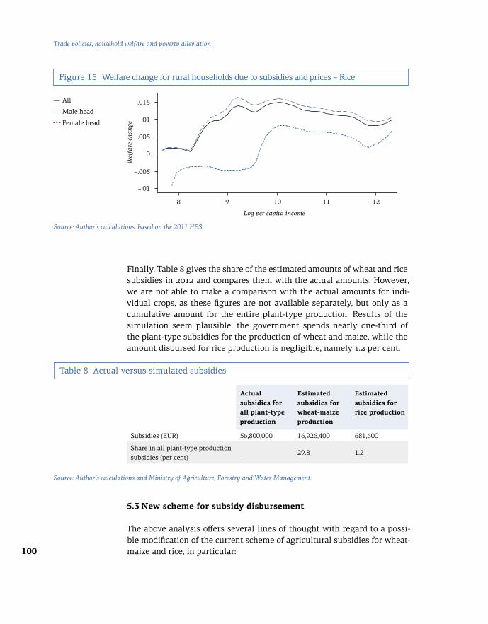
100
Trade policies, household welfare and poverty alleviation
Figure 15 Welfare change for rural households due to subsidies and prices – Rice
Source: Author’s calculations, based on the 2011 HBS.
Finally, Table 8 gives the share of the estimated amounts of wheat and rice subsidies in 2012 and compares them with the actual amounts. However, we are not able to make a comparison with the actual amounts for indi-vidual crops, as these figures are not available separately, but only as a cumulative amount for the entire plant-type production. Results of the simulation seem plausible: the government spends nearly one-third of the plant-type subsidies for the production of wheat and maize, while the amount disbursed for rice production is negligible, namely 1.2 per cent.
Table 8 Actual versus simulated subsidies
Source: Author’s calculations and Ministry of Agriculture, Forestry and Water Management.
Actual subsidies for all plant-type production
Estimated subsidies for wheat-maize production
Estimated subsidies for rice production
Subsidies (EUR) 56,800,000 16,926,400 681,600
Share in all plant-type production subsidies (per cent)
- 29.8 1.2
5.3 New scheme for subsidy disbursement
The above analysis offers several lines of thought with regard to a possi-ble modification of the current scheme of agricultural subsidies for wheat-maize and rice, in particular:
.015
.01
0
.005
–.005
–.01
Wel
fare
cha
nge
Log per capita income
8 9 10 11 12
― All
– – Male head
Female head

101
FYR
OM
Increasing the welfare effect of the agricultural subsidy programme for food crop production in the FYROM
Table 9 New proposed scheme for subsidy disbursement
Source: Author.
• The poorest female-headed rural households should be targeted more intensively to encourage them to produce wheat and maize, especially because of the large effect that production may have on the welfare of this group along income distribution.
• All rice producers should be targeted with possibly larger subsidies per cultivated hectare and with a more intensive targeting of the poorest households.
• Poorest urban households (largely defined as those in the first two quintiles of the income distribution) should also be a target of the pro-gramme for wheat and maize (rice production being rather specific due to the difficulty of the production process and the climatic conditions it requires). The programme should target in particular the female-head-ed households, given the possibility to accompany it by a usufruct of state-owned land11 and one-off subsidies for purchase of the minimum equipment for agricultural production. These instruments may attract urban dwellers, and particularly former rural-urban migrants, to get them involved in agricultural production.
Given these findings, we propose the following new scheme for subsidy disbursement, presented in Table 9.
11 According to the official numbers from the Ministry of Agriculture, Forestry and Water Management, about 48 per cent of the entire land in the former Yugoslav Republic of Macedonia is agricultural land (about one million ha). The state owns about 20 per cent – i.e. about 200,000 ha – of the arable land.
Wheat/Maize Rice
All households– Reduction of the subsidy to EUR 110 per ha
All households– Increase of the subsidy to EUR 250 per ha
Female-headed rural households with per capita income of less than EUR 220 – Increase of the subsidy to EUR 185 per ha
Female-headed rural households with per capita income of less than EUR 360 – Increase of the subsidy to EUR 375 per ha
All urban households with per capita income of less than EUR 360– Subsidy of EUR 100 per ha– State-owned land up to 1.15 ha at usufruct– Initial lump sums for investment into min-imal machinery for agricultural production
Male-headed rural households with per capita income of less than EUR 80 – Increase of the subsidy to EUR 375 per ha
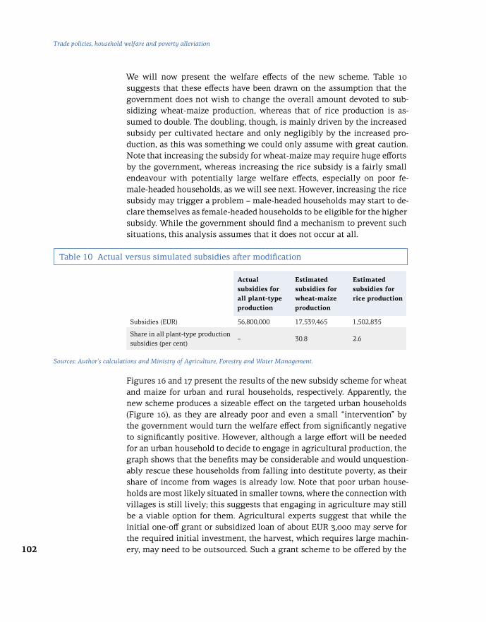
102
Trade policies, household welfare and poverty alleviation
We will now present the welfare effects of the new scheme. Table 10 suggests that these effects have been drawn on the assumption that the government does not wish to change the overall amount devoted to sub-sidizing wheat-maize production, whereas that of rice production is as-sumed to double. The doubling, though, is mainly driven by the increased subsidy per cultivated hectare and only negligibly by the increased pro-duction, as this was something we could only assume with great caution. Note that increasing the subsidy for wheat-maize may require huge efforts by the government, whereas increasing the rice subsidy is a fairly small endeavour with potentially large welfare effects, especially on poor fe-male-headed households, as we will see next. However, increasing the rice subsidy may trigger a problem – male-headed households may start to de-clare themselves as female-headed households to be eligible for the higher subsidy. While the government should find a mechanism to prevent such situations, this analysis assumes that it does not occur at all.
Table 10 Actual versus simulated subsidies after modification
Sources: Author’s calculations and Ministry of Agriculture, Forestry and Water Management.
Actual subsidies for all plant-type production
Estimated subsidies for wheat-maize production
Estimated subsidies for rice production
Subsidies (EUR) 56,800,000 17,539,465 1,502,835
Share in all plant-type production subsidies (per cent)
– 30.8 2.6
Figures 16 and 17 present the results of the new subsidy scheme for wheat and maize for urban and rural households, respectively. Apparently, the new scheme produces a sizeable effect on the targeted urban households (Figure 16), as they are already poor and even a small “intervention” by the government would turn the welfare effect from significantly negative to significantly positive. However, although a large effort will be needed for an urban household to decide to engage in agricultural production, the graph shows that the benefits may be considerable and would unquestion-ably rescue these households from falling into destitute poverty, as their share of income from wages is already low. Note that poor urban house-holds are most likely situated in smaller towns, where the connection with villages is still lively; this suggests that engaging in agriculture may still be a viable option for them. Agricultural experts suggest that while the initial one-off grant or subsidized loan of about EUR 3,000 may serve for the required initial investment, the harvest, which requires large machin-ery, may need to be outsourced. Such a grant scheme to be offered by the

103
FYR
OM
Increasing the welfare effect of the agricultural subsidy programme for food crop production in the FYROM
government is comparable with the current scheme for support of sin-gle-employee start-ups, and may be considered together.
Targeted female-headed rural households (Figure 17) may also reap large benefits but only if they decide for a larger-scale production. Namely, the graph assumes that these households would expand wheat-maize sown land from the present low amounts to at least an average of about 1.15 cul-tivated hectares. If this is the case, the poorest female-headed rural house-holds may increase the welfare effect of the scheme from virtually zero to about two-thirds of the income of their male counterparts. However, this assumption is rather strong, given our findings that subsidies do not in-crease production, and should therefore be approached with considerable caution.
Although the current scheme does not likely have an effect on produc-tion, the new scheme we propose may start influencing production due to the provision of larger subsidies for specific households. In addition, one should bear in mind that the results are also conditional on resolving two important issues: (a) declaring the household as female-headed when it is actually male-headed to qualify for a higher subsidy; and (b) traditionally lower participation of women in production activities.
Figure 16 Welfare change for urban households after scheme modification – Wheat and maize
Source: Author’s estimations.
.4
.2
.3
.1
0
8 9 10 11 12 13
Wel
fare
cha
nge
Log per capita income
― All
– – Male head
Female head

104
Trade policies, household welfare and poverty alleviation
Figure 17 Welfare change for rural households after scheme modification – Wheat and maize
Source: Author’s estimations.
Figure 18 presents the results of the new subsidy scheme for rice for rural households only. There are two important caveats with regard to the cul-tivation of rice and subsequently to the proposed scheme. First, although urban households were found to be negatively affected by the rice price increase, it is unlikely that they can be steered to produce rice even if of-fered free-of-charge state-owned land or additional subsidies for initial in-vestment in machinery. This is due to the specificity of rice production. Second, the proposed scheme targets all rural households (producers and non-producers). This seems ambitious because rice production requires specific climate for production (specific regions of the country), in addi-tion to the particularities of the production process (for instance, plant-ing rice under water). From that viewpoint, the results presented in Figure 18 seem to overestimate the welfare impact of the new subsidy scheme. Unfortunately, we do not have the regional information in the survey that would allow us to target the regions known for rice production only. Still, the information obtained in Figure 18 is valuable, as it suggests that the effects of a well-targeted subsidy programme for rice may be sizeable, as-suming that the considerably larger subsidy per hectare offered will mo-tivate poor households that otherwise cultivate smaller plots of land to increase production. For the poor female-headed rural households, the overall welfare effect turns from slightly negative to significantly positive, and with a considerable share of rice income in overall income, due to the low initial income level.
1.5
1
.5
0
8 9 10 11 12
Wel
fare
cha
nge
Log per capita income
― All
– – Male head
Female head

105
FYR
OM
Increasing the welfare effect of the agricultural subsidy programme for food crop production in the FYROM
Figure 18 Welfare change for rural households after scheme modification – Rice
Source: Author’s estimations.
6 Conclusions and policy recommendations
The objective of this study was to analyse the welfare implications of ris-ing prices of wheat, maize and rice and those of agricultural subsidies on household welfare in the former Yugoslav Republic of Macedonia. We used the 2011 Household Budget Survey data and non-parametric tech-niques to estimate these effects on household welfare along the segments of the income distribution.
Results suggest that increasing prices of wheat, maize and rice exerted positive welfare effects on male-headed rural households only, whereas the effects on female-headed rural households and all urban households were generally negative, largely due to the different production patterns. The welfare effect of the government subsidy programme for wheat and maize production was positive for all rural households: fairly large for male-headed households and small for female-headed rural households. The effect on rice production was zero or negligible, largely due to the small subsidy amount versus the large effort needed for the cultivation of rice. Overall, both price and subsidy effects were found positive only for the male-headed rural households.
Based on these findings, we evaluated a new disbursement scheme for government subsidies targeting female-headed rural households for both crops (wheat-maize and rice); all poor urban households for wheat; and
.25
.2
.1
.15
.05
0
Wel
fare
cha
nge
Log per capita income
8 9 10 11 12
― All
– – Male head
Female head

106
Trade policies, household welfare and poverty alleviation
male-headed rural households for rice. For the poor urban households, we also proposed the possibility of a usufruct of state-owned land and initial subsidy for investment in machinery; for the poor rural rice producers, we proposed an effort to steer non-producers to become engaged in produc-tion where possible, along with a larger subsidy per cultivated hectare. However, the simulation setup is largely based on re-distributional effects and only modestly on increased production effects, as we were unable to document that subsidies positively affected cereal production in the for-mer Yugoslav Republic of Macedonia.
Results of the simulation suggest that targeting poor urban households for wheat-maize production could result in a significant welfare effect rang-ing up to 30–40 per cent of the initial income of this group of households. Targeting poor female-headed rural households may increase the impact of the scheme to about two-thirds of the income of poor male-headed ru-ral households, preventing this vulnerable group from falling into desti-tute poverty. The effect on poor rural rice producers may also be large – up to 20 per cent of household income – taking into account that a consider-able effort is however needed to start off rice production.
Hence, the policy recommendations stemming from this analysis dovetail to putting particular emphasis on poor female-headed rural households for both wheat-maize and rice production, increasing the subsidy for rice pro-duction due to its specificity and large effort needed, and offering the usu-fruct of state-owned land and start-off grants for poor urban households to encourage them to produce wheat and maize.
Although this analysis was motivated by the fact that the government uses subsidies to target the poor, it abstracts from discussing other more direct means to address poverty in the economy. Other policies would include so-cial financial assistance schemes, in-work benefits, conditional cash trans-fers and the like. Even though the interplay of those policies with the agricultural subsidies programme may be interesting to analyse, it re-mains a topic for future research and discussion.

107
FYR
OM
Increasing the welfare effect of the agricultural subsidy programme for food crop production in the FYROM
Figure A1.1 Components of the welfare function of urban households in 2006 – Wheat and maize
Source: Author’s estimations, based on the 2011 HBS.
Annex
Annex 1: Detailed diagrams – Price change for wheat and maize
.08
.00004
.00005
.6
.8
.4
.3
.04
.00002
.2
.1
.06
.00003
.4
.2
.02
.00001
0
0
0
0
–.1
8
8
8
8
9
9
9
9
10
10
10
10
11
11
11
11
12
12
12
12
13
13
13
13
Shar
eSh
are
Shar
eSh
are
Log per capita income
Labour income
Wheat-maize expenditure
Wheat-maize net
Wheat-maize income
Log per capita income
Log per capita income
Log per capita income
― All
– – Male head
Female head
― All
– – Male head
Female head
― All
– – Male head
Female head
― All
– – Male head
Female head

108
Trade policies, household welfare and poverty alleviation
Figure A1.2 Components of the welfare function of rural households in 2006 – Wheat and maize
Source: Author’s estimations, based on the 2011 HBS.
.4
2
.6
.2
1
.2
1
.3
1.5
.4
1.5
.1
.5
.5
0
0
0
0
Shar
eSh
are
Shar
eSh
are
Log per capita income
Log per capita income
Log per capita income
Log per capita income
― All
– – Male head
Female head
― All
– – Male head
Female head
― All
– – Male head
Female head
― All
– – Male head
Female head
8
8
8
8
9
9
9
9
10
10
10
10
11
11
11
11
12
12
12
12
Labour income
Wheat-maize expenditure
Wheat-maize net
Wheat-maize income
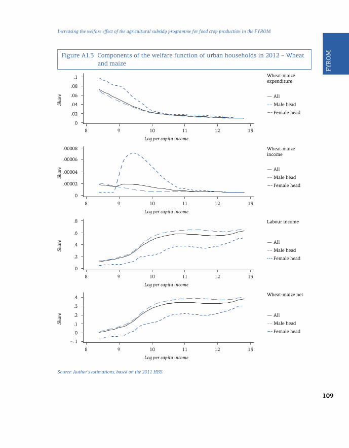
109
FYR
OM
Increasing the welfare effect of the agricultural subsidy programme for food crop production in the FYROM
Figure A1.3 Components of the welfare function of urban households in 2012 – Wheat and maize
Source: Author’s estimations, based on the 2011 HBS.
.1
.08
.00006
.00008
.6
.8
.4
.3
.04
.00004
.2
.1
.06
.4
.2
.02
.00002
0
0
0
0
–. 1
8
8
8
8
9
9
9
9
10
10
10
10
11
11
11
11
12
12
12
12
13
13
13
13
Shar
eSh
are
Shar
eSh
are
Log per capita income
Log per capita income
Log per capita income
Log per capita income
― All
– – Male head
Female head
― All
– – Male head
Female head
― All
– – Male head
Female head
― All
– – Male head
Female head
Labour income
Wheat-maize expenditure
Wheat-maize net
Wheat-maize income

110
Trade policies, household welfare and poverty alleviation
Figure A1.4 Components of the welfare function of rural households in 2012 – Wheat and maize
Source: Author’s estimations, based on the 2011 HBS.
.5
.4
3
.6
.2
2
.2
1
1.5
.3
.4
2
.1
1
.5
0
0
0
0
Shar
eSh
are
Shar
eSh
are
Log per capita income
Log per capita income
Log per capita income
Log per capita income
― All
– – Male head
Female head
― All
– – Male head
Female head
― All
– – Male head
Female head
― All
– – Male head
Female head
8
8
8
8
9
9
9
9
10
10
10
10
11
11
11
11
12
12
12
12
Labour income
Wheat-maize expenditure
Wheat-maize net
Wheat-maize income

111
FYR
OM
Increasing the welfare effect of the agricultural subsidy programme for food crop production in the FYROM
Figure A2.1 Components of the welfare function of urban households in 2006 – Rice
Annex 2: Detailed diagrams – Price change for rice
Source: Author’s estimations, based on the 2011 HBS.
.05
.04
.00015
.6
.8
.4
.3
.02
.0001
.2
.1
.03
.4
.2
.01
.00005
0
0
0
0
–.1
8
8
8
8
9
9
9
9
10
10
10
10
11
11
11
11
12
12
12
12
13
13
13
13
Shar
eSh
are
Shar
eSh
are
Log per capita income
Log per capita income
Log per capita income
Log per capita income
― All
– – Male head
Female head
― All
– – Male head
Female head
― All
– – Male head
Female head
― All
– – Male head
Female head
Labour income
Rice expenditure
Rice net
Rice income

112
Trade policies, household welfare and poverty alleviation
Figure A2.2 Components of the welfare function of rural households in 2006 – Rice
Source: Author’s estimations, based on the 2011 HBS.
.025
.02
.05
.6
.01
.03
.04
.2
.2
.3
.015
.4
.4
.005
.02
.1
0
0
.01
0
0
Shar
eSh
are
Shar
eSh
are
Log per capita income
Log per capita income
Log per capita income
Log per capita income
― All
– – Male head
Female head
― All
– – Male head
Female head
― All
– – Male head
Female head
― All
– – Male head
Female head
8
8
8
8
9
9
9
9
10
10
10
10
11
11
11
11
12
12
12
12
Labour income
Rice expenditure
Rice net
Rice income

113
FYR
OM
Increasing the welfare effect of the agricultural subsidy programme for food crop production in the FYROM
Figure A2.3 Components of the welfare function of urban households in 2012 – Rice
Source: Author’s estimations, based on the 2011 HBS.
.08
.06
.04
.00015
.0002
.6
.8
.4
.3
.02
.0001
.2
.1
.4
.2
.00005
0
0
0
0
–.1
8
8
8
8
9
9
9
9
10
10
10
10
11
11
11
11
12
12
12
12
13
13
13
13
Shar
eSh
are
Shar
eSh
are
Log per capita income
Log per capita income
Log per capita income
Log per capita income
― All
– – Male head
Female head
― All
– – Male head
Female head
― All
– – Male head
Female head
― All
– – Male head
Female head
Labour income
Rice expenditure
Rice net
Rice income
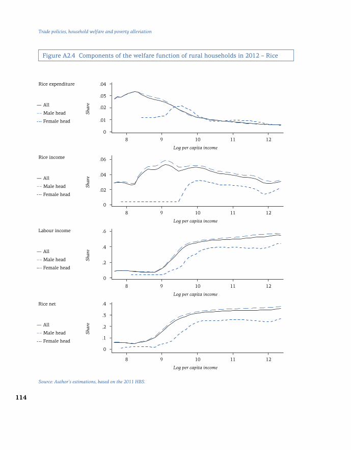
114
Trade policies, household welfare and poverty alleviation
Figure A2.4 Components of the welfare function of rural households in 2012 – Rice
Source: Author’s estimations, based on the 2011 HBS.
.04
.06
.6
.02
.04
.2
.2
.3
.03
.4
.4
.01
.02
.1
0
0
0
0
Shar
eSh
are
Shar
eSh
are
Log per capita income
Log per capita income
Log per capita income
Log per capita income
― All
– – Male head
Female head
― All
– – Male head
Female head
― All
– – Male head
Female head
― All
– – Male head
Female head
8
8
8
8
9
9
9
9
10
10
10
10
11
11
11
11
12
12
12
12
Labour income
Rice expenditure
Rice net
Rice income

115
FYR
OM
Increasing the welfare effect of the agricultural subsidy programme for food crop production in the FYROM
References
Aksoy, A. and Isik-Dikmelik, A. (2008). “Are Low Food Prices Pro-Poor? Net Food Buyers and Sellers in Low-Income Countries.” Policy Research Working Paper No. 4642. World Bank, Washington DC.
Baltagi, B.H. (2008). Econometric Analysis of Panel Data. Fourth Edition. Chichester: Wiley.
Barrett, C.D. and Dorosh, P.A. (1996). “Farmers’ Welfare and Changing Food Prices: Nonparametric Evidence from Rice in Madagascar.” American Journal of Agricultural Economics, 78 (3): 656–669.
Budd, J.W. (1993). “Changing Food Prices and Rural Welfare: A Non-Parametric Examination of the Cote d’Ivoire.” Economic Development and Cultural Change, 41 (3): 587–603.
Christiaensen, L. and Demery, L. (2007). Down to Earth: Agriculture and Poverty Reduction in Africa. World Bank, Washington DC. Available at: http://siteresources.worldbank.org/INTPOVERTY/Resources/335642-1130251872237/DownToEarth_final.pdf.
de Hoyos, R.E. and Medvedev, D. (2011). “Poverty Effects of Higher Food Prices. A Global Perspective.” Review of Development Economics, 15 (3): 387–402.
Deaton, A. (1989a). “Rice Prices and Income Distribution in Thailand: A Non-Parametric Analysis.” The Economic Journal, 99 (395): 1–37.
Deaton, A. (1989b). “Household Survey Data and Pricing Policies in Developing Countries.” The World Bank Economic Review, 3 (2): 183–210.
Deaton, A. (1997). The Analysis of Household Surveys. A Microeconometric Approach to Development Policy. Baltimore and Washington DC: Johns Hopkins University Press and World Bank.
FAO (2011). How does international price volatility affect domestic economies and food security? Food and Agriculture Organization of the United Nations, Rome.
Friedman, J. and Levinsohn, J. (2002). “The distributional impacts of Indonesia’s financial crisis on household welfare: a ‘rapid response’ methodology.” The World Bank Economic Review, 16 (3): 397–423.
Hertel, T. and Winters, L.A. Ed. (2006). Poverty and the WTO: Impacts of the Doha Development Agenda. Basingstoke and Washington DC: Palgrave Macmillan and World Bank.
Ivanic, M. and Martin W. (2008). “Implications of Higher Global Food Prices for Poverty in Low-Income Countries.” Agricultural Economics, 39 (s1): 405–416.
Jovanovic, B. and Petreski, M. (2012). “Hemlock for policy response: Monetary policy, exchange rates and labour un-ions in SEE and CIS during the crisis.” FIW Working Paper Series No. 081. Forschungsschwerpunkt Internationale Wirtschaft, Vienna.
Klytchnikova, I. and Diop, N. (2010). “Trade Reforms, Farm Productivity, and Poverty in Bangladesh.” In: Aksoy, M.A. and Hoekman B. Eds. Food Prices and Rural Poverty. World Bank, Washington DC.
Poulton, C., Kyddd, J., Wiggins, S. and Dorward, A. (2006). “State interventions for food price stabilization in Africa: Can it Work?” Food Policy, 31: 342–356.

116
Trade policies, household welfare and poverty alleviation
Ravallion, M. (1990). “Rural welfare changes of food prices under induced wage responses: Theory and evidence from Bangladesh.” Oxford Economic Papers, 42: 574–585.
Ravallion, M. and van de Walle, D. (1991). “The impact on poverty of food pricing reforms: A welfare analysis for Indonesia.” Journal of Policy Modeling, 13 (2): 281–299.
Singh, I., Squire, L. and Strauss, J. (1986). Agricultural Household Models: Extensions and Applications. Baltimore: Johns Hopkins University Press.
Wodon, Q. and Zaman, H. (2010). “Rising Food Prices in Sub-Saharan Africa: Poverty Impact and Policy Responses.” World Bank Research Observer, 25 (1): 157–176.
Wodon, Q., Tsimpo, C., Backiny-Yetna, P., Joseph, G., Adoho, F. and Coulombe, H. (2008). “Potential Impact of Higher Food Prices on Poverty: Summary Estimates for a Dozen West and Central African Countries.” Policy Research Working Paper No. 4745. World Bank, Washington DC.
Wooldridge, J.M. (2002). Econometric Analysis of Cross Section and Panel Data. Cambridge MA: MIT Press.
World Bank (2008). High food prices: a harsh new reality [online]. Available at: http://econ.worldbank.org/WBSITE/EXTERNAL/EXTDEC/0,,contentMDK:21665883~pagePK:64165401~piPK:64165026~theSitePK:469372,00.html.

117
FYR
OM
Increasing the welfare effect of the agricultural subsidy programme for food crop production in the FYROM

118
Trade policies, household welfare and poverty alleviation
Argentina

119
Arg
enti
naWelfare impact of wheat export restrictions in Argentina: Non-parametric analysis on urban households
Abstract
The Argentine wheat value chain was subject to considerable policy inter-ventions during the last decade. The measures adopted by the government included export duties from 2002 onward, quantitative wheat export re-strictions since 2006, and domestic price ceilings and subsidies introduced in 2007. These policy instruments aimed to limit the increase in domestic prices of cereals during a period of high international prices and to keep an adequate provision of grains in the domestic market. Export restric-tions implicitly intended to avoid an increase in the prices of basic con-sumption goods derived from wheat. However, these non-tariff measures could also distort farmers’ incentives to produce. Using non-parametric techniques, this study contributes to the policy discussion of the effects of non-tariff measures in the cereals market by evaluating the welfare impact of wheat export restrictions on Argentine urban households. Focusing on the effects of changes in prices of final consumption goods during 2006–2011, the study finds that prices of wheat derivatives would be only 1 per cent higher in the absence of quantitative restrictions, with negligible wel-fare effects on consumers. If both export restrictions and subsidies to mill-ers were removed, prices would be 6.4 per cent higher. This would imply modest welfare losses ranging from zero to 1.5 per cent, mainly affecting the poorest households.
Paula Andrea Calvo *
* The author would like to thank Raúl Auger from the National Senate of Argentina and Roberto Bisang from Universidad de Buenos Aires for their support in the preparation of this study.

120
Trade policies, household welfare and poverty alleviation
1 Introduction
In 2006, the Argentine government initiated a succession of temporal ex-port prohibitions and quotas on exports of wheat and corn, which were added to high export duties applied since 2002. These non-tariff measures (NTMs) became one of the most important trade policies of the incumbent government. Moreover, a broad set of complementary measures, includ-ing ceiling prices and subsidies, were put into practice, aiming to influence the price of cereals and their derivatives in the domestic market. The re-sult was a complex system of interventions in the value chain of wheat, po-tentially distorting prices and incentives in different stages of production.1
These policy measures generated an intense debate between those in fa-vour and those against them. Supporters argued that export restrictions limited the increase in domestic prices of grains by shielding domestic prices from high levels prevailing in international markets. According to the World Bank Commodities Price Data,2 prices of agricultural commod-ities increased by 137 per cent in nominal terms between 2002 and 2012. Food prices increased more than did raw materials (152 per cent versus 116 per cent). In particular, nominal prices of wheat increased by 112 per cent during this period.3
Final products – such as bakery products and pasta – that use wheat as an input in production are an important component of the basic food basket of the typical Argentine household.4 Consequently, the policies
1 Many countries implemented policies to restrict food exports as a response to the price spikes of 2007–2008. This led to a further increase in commodity prices in international markets. As a result, export restrictions were placed on the agenda of multilateral negotia- tions in an attempt to address high and volatile food prices (Sharma, 2011). 2 The Commodities Price Data (also known as “Pink Sheet”) are a monthly collection of commodity prices and indices published by the World Bank. See http://econ.worldbank.org/ WBSITE/EXTERNAL/EXTDEC/EXTDECPROSPECTS/0,,contentMDK:215749 07~menuPK:7859231~pagePK:64165401~piPK:64165026~theSitePK:476883,00.html. 3 Key reasons behind the spike in commodity prices during the last decade have been extensively discussed in the literature. Possible explanations can be found in the growth of the world economy until 2008, followed by an increase in demand (especially in the People’s Republic of China and India), the increasing role of commodities in financial portfolios, and depreciation of the dollar. Also, the higher use of food commodities in biodiesel industries and climatic factors could have contributed to the price boom (Gayá and Michalczewsky, 2011; Gilbert, 2010; Abbott et al., 2011; Cooke and Robles, 2009; Mitchell, 2008). The increasing role of commodities in financial portfolios has made commodity prices more responsive to financial conditions. As suggested by UNCTAD (2012), financialization is the root cause of commodity price volatility. This would help explain the impressive growth in commodity prices until 2008, the collapse during the 2009 crisis and the subsequent recovery of prices.

121
Arg
enti
na
Welfare impact of wheat export restrictions in Argentina: Non-parametric analysis on urban households
4 Derivatives of wheat have an important share in official consumer price index (CPI) calculations. For CPI 1999=100, the group Food and Beverages had a share of 31.28 per cent of CPI, whereas the subgroup Bread, Cereals and Pasta had a weight of 4.54 per cent. Currently, in CPI 2008=100, Food and Beverages have a share of 37.8 per cent and Bread, Cereals and Pasta have a weight of 7.14 per cent. 5 See Ministry of Economy and Production, Resolution 9/2007. 6 Data from the Buenos Aires Futures Exchange Market and the World Bank Commodities Price data indicate that the average price in the domestic market was USD 463 and the international price USD 307 per metric ton.
explicitly aimed to limit price increases in a setting of high inflation rates in Argentina. Moreover, they aimed to keep an adequate supply of grains in the domestic market in a setting of growing international demand and weather-induced national shortages. Thus, although these measures could hurt producers, export restriction could benefit consumers.5
Opponents of these policies argued that grains only play a small role in price formation of final goods compared to other components such as wag-es, utilities, taxes, freights, etc. Controls on cereal prices would thus not be sufficient to limit inflation. Additionally, export restrictions could po-tentially affect producer incentives, thus reducing the supply of cereals in the domestic market. For example, restrictions on wheat exports could mo-tivate producers to divert land to more profitable crops, such as barley or sorghum. By exporting these grains, producers could circumvent the re-strictive policies imposed by the government and take advantage of the fa-vourable external conditions. If that were the case, the potential positive effect of policies on consumers could become negligible, as a lower sup-ply would have the opposite effect on domestic prices. The evidence sug-gests some trends in this direction. According to data from the Ministry of Agriculture, between 2006 and 2012, the wheat-sown area indeed de-creased by 44.3 per cent. Also, in September 2013, domestic wheat prices were 50 per cent higher than international prices.6
This study aims to contribute to the current discussion on the impacts of interventions in the wheat market through the application of NTMs. Following Deaton (1989a, 1989b) and Benjamin and Deaton (1993), it uses non-parametric techniques to capture the effect of export restrictions on wheat on household welfare. The analysis focuses on welfare changes op-erating through changes in prices of final goods that use wheat as a produc-tion input and represent an important component of the basic consumption basket. Estimations of welfare gains or losses of the policies are based on a comparison of consumer welfare under the real scenario against several counterfactual scenarios. The analysis focuses on the “post-intervention” period 2006–2011 when NTMs were implemented. The “pre-intervention”
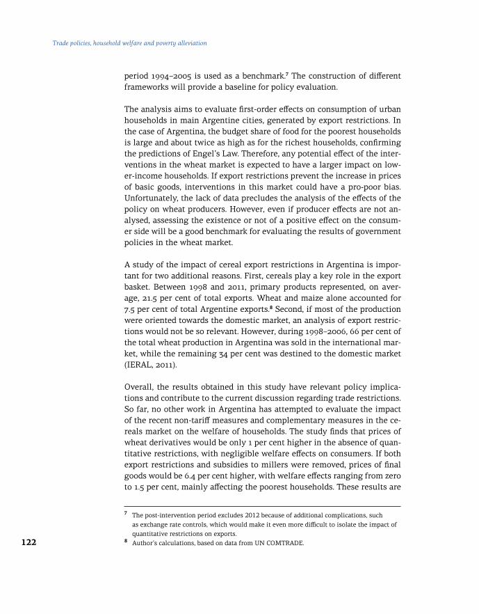
122
Trade policies, household welfare and poverty alleviation
period 1994–2005 is used as a benchmark.7 The construction of different frameworks will provide a baseline for policy evaluation.
The analysis aims to evaluate first-order effects on consumption of urban households in main Argentine cities, generated by export restrictions. In the case of Argentina, the budget share of food for the poorest households is large and about twice as high as for the richest households, confirming the predictions of Engel’s Law. Therefore, any potential effect of the inter-ventions in the wheat market is expected to have a larger impact on low-er-income households. If export restrictions prevent the increase in prices of basic goods, interventions in this market could have a pro-poor bias. Unfortunately, the lack of data precludes the analysis of the effects of the policy on wheat producers. However, even if producer effects are not an-alysed, assessing the existence or not of a positive effect on the consum-er side will be a good benchmark for evaluating the results of government policies in the wheat market.
A study of the impact of cereal export restrictions in Argentina is impor-tant for two additional reasons. First, cereals play a key role in the export basket. Between 1998 and 2011, primary products represented, on aver-age, 21.5 per cent of total exports. Wheat and maize alone accounted for 7.5 per cent of total Argentine exports.8 Second, if most of the production were oriented towards the domestic market, an analysis of export restric-tions would not be so relevant. However, during 1998–2006, 66 per cent of the total wheat production in Argentina was sold in the international mar-ket, while the remaining 34 per cent was destined to the domestic market (IERAL, 2011).
Overall, the results obtained in this study have relevant policy implica-tions and contribute to the current discussion regarding trade restrictions. So far, no other work in Argentina has attempted to evaluate the impact of the recent non-tariff measures and complementary measures in the ce-reals market on the welfare of households. The study finds that prices of wheat derivatives would be only 1 per cent higher in the absence of quan-titative restrictions, with negligible welfare effects on consumers. If both export restrictions and subsidies to millers were removed, prices of final goods would be 6.4 per cent higher, with welfare effects ranging from zero to 1.5 per cent, mainly affecting the poorest households. These results are
7 The post-intervention period excludes 2012 because of additional complications, such as exchange rate controls, which would make it even more difficult to isolate the impact of quantitative restrictions on exports. 8 Author’s calculations, based on data from UN COMTRADE.

123
Arg
enti
na
Welfare impact of wheat export restrictions in Argentina: Non-parametric analysis on urban households
9 This figure is based on World Bank data on a poverty headcount ratio of USD 2 a day, adjusted by purchasing power parity (PPP), at 2005 international prices. 10 See Ministry of Economy, Resolution 11/2002.
indicative of the failure of the policies to achieve welfare goals, and might help direct the design and implementation of future policies.
The study is organized as follows. Section 2 describes in detail the broad set of policies implemented in the wheat market during the last years and discusses the role of wheat in the Argentine economy. Section 3 summa-rizes the literature associated with the use of non-parametric techniques to address welfare effects of commodity prices on poverty. Data and meth-odology are presented in Section 4. Section 5 discusses the main results, and Section 6 concludes.
2 Wheat: Value chain and intervention policies
This section describes the general situation and the policies implemented in Argentina’s wheat market. It also briefly discusses the implications of the recent policy interventions for the value chain of wheat.
In 1999, Argentina entered a recession that triggered a decline of gross domestic product (GDP), investment and consumption in real terms. The situation worsened during 2001, culminating in one of the worst crises in Argentina’s history. Between 1998 and 2002, GDP at constant prices fell by 18 per cent. In January 2002, the Convertibility Law was abolished, with a consequent nominal devaluation of the Argentine peso (ARS) by 140 per cent during the first quarter of 2002. Social indicators were also strong-ly affected by the crisis: in 2002, the poverty rate peaked at 23 per cent9 while the unemployment rate rose to 21.5 per cent in the first half of that year. Favourable external conditions helped to overcome the crisis and drove the improved performance of the economy in the following years. The increase in commodity prices, coupled with real exchange rate depre-ciation, fostered agricultural exports. At the same time, the government had an urgent need to raise funds to address the widespread social crisis.10 In February 2002, export duties on cereals, oil seeds and their derivatives were introduced – the first of a large set of policy measures applied to ce-reals and oil seeds during the last decade.
To better understand the impact of the measures that were implemented, it is important to understand the organization of the value chain of wheat. The chain consists of three stages: (a) primary production (sowing and

124
Trade policies, household welfare and poverty alleviation
harvesting of the grain); (b) first processing stage during which the mill-ing industry transforms wheat into wheat flour as the main output; and (c) second processing stage during which the industry uses wheat outputs processed in the first stage as main inputs. The outputs of this third stage are mainly bakery products (especially bread), cookies, biscuits and pas-ta. The wheat value chain has been frequently targeted by government in-terventions, partly because of the importance of wheat-based products in Argentine household consumption, and partly because of the traditional competing role of the agricultural sector and the manufacturing industry in the design of Argentina’s trade policy.11
During the 1980s, the cereals market was a target of several policies, such as high export duties and exchange rate control, which affected grain pro-ducer incentives due to domestic prices being well below international prices. During the 1990s, the wheat market was deregulated, reducing the gap between national and international prices of grain (Ghezán et al., 2001). However, as discussed above, the government re-intervened in the wheat market in the early 2000s, affecting supply and prices in the domestic market.
The text that follows summarizes the most important policies implement-ed in the wheat value chain during the last decade.
Tariff measures
Export duties were first implemented in February 2002, at 10 per cent for wheat, 5 per cent for wheat flour and other mixes for bakery, and 5 per cent for bakery products, cookies and pasta.12 The implementation of ex-port duties was motivated by fiscal reasons, in an attempt to raise funds to finance the government budget. The rates were changed several times before reaching, in January 2009, their current values of 23 per cent for wheat, 13 per cent for wheat flour and 5 per cent for second processing stage products (IERAL, 2011; Peri, 2009).13
11 Brambilla et al. (2010) highlight the role of distributional conflict as a key determinant of trade policy in Argentina. In particular, there is a natural tension between the sector with a comparative advantage (agriculture), represented by landowners, and the industry, which is the domain of workers. In this scenario, a free trade policy, other things being equal, worsens the distribution of income in Argentina. 12 See Ministry of Economy, Resolution 11/2002. 13 In March 2008, Resolution 125 of the Ministry of Economy tied export duties of wheat, corn, soybean and sunflower to free on board (FOB) prices of grains and oil seeds to adjust rates automatically as international prices increased. This law was derogated in July 2008 after a conflict between the government and rural workers and organizations, which included lock-outs and suspension of grain commercialization for more than 120 days.

125
Arg
enti
na
Welfare impact of wheat export restrictions in Argentina: Non-parametric analysis on urban households
14 Quantitative export restrictions were imposed only on the export of grains and did not affect the export of wheat-based products (such as flour and cookies). 15 ONCCA stands for Oficina Nacional de Control Comercial Agropecuario. 16 See ONCCA, Resolution 543/2008. 17 These time periods, ranging from 45 days to one year, were also modified several times. 18 See ONCCA, Resolutions 2846/2008, 2/2009 and 5556/2009; AFIP (Administración Federal de Ingresos Públicos – the Federal Administration of Public Revenue), Resolution 2636.
Non-tariff measures
These measures consist of quantitative restrictions (export quotas) on wheat exports. They were first implemented in May 2006, with temporary halts of grain export.14 They were then strengthened in May 2008 through the Register of Export Operations (ROE) for agricultural products (called the “Green ROE”), a system of non-automatic export licences administered by the National Office of Control of Agricultural Trade (ONCCA).15 The sys-tem of restrictions was based on the calculation of an exportable surplus, defined as a function of the total availability of grains and the needs of the domestic industry, adjusted by a factor meant to cover potential con-tingencies. If the exportable surplus were zero, exports would be prohibit-ed.16 Calculations of quotas and requirements of the domestic market were modified several times, creating uncertainty for producers and exporters and affecting their decision-making process. Each November, the ONCCA determined domestic market requirements and the amount that each firm could export, as a function of the firm’s performance in the previous year. In addition, several complementary administrative procedures were intro-duced, potentially hindering commercialization. Among them was a reduc-tion of the time period during which exporters could sell the product in the external market after receiving approval.17 Also, exporters had to pay export duties in advance.18
Compensation regime for the wheat milling industry and producers
In 2007, export restrictions were complemented with a compensation scheme consisting of ceiling prices and subsidies for the wheat milling in-dustry and producers. These measures intended to control prices of wheat derivatives in the domestic market. The compensation regime established an “internal supply price” that millers should pay in the domestic mar-ket, with the aim of controlling the price of bread and bakery products. In cases where the prices paid by millers in the domestic market exceed-ed the internal supply price, which was set at an artificially low level, the

126
Trade policies, household welfare and poverty alleviation
law provided a subsidy covering the price differential.19 The policy also in-cluded a compensation scheme for grain producers to guarantee that they would benefit from the increase in prices in international markets. The amount of the subsidy was calculated as the difference between the theo-retical free alongside ship (FAS)20 price and the sales price in the domestic market. The subsidy to producers applied to 85 per cent of declared inter-nal sales.21
Figure 1 illustrates the effects of the compensation scheme. The system generated a double price gap in the wheat market to be covered by subsi-dies. The lower gap in Figure 1 shows the difference between the domestic wheat price and the internal supply price, which was covered by subsi-dies to the milling industry. This gap was large during most of the an-alysed period, imposing a heavy burden on the government budget. The upper gap shows the difference between the theoretical FAS price and the domestic price of wheat. In theory, this difference should have been cov-ered by subsidies to producers. In practice, however, subsidies to produc-ers were mostly not paid or were disbursed with several months of delay. This upper gap represents a loss for producers who were not able to take advantage of favourable external conditions (even after adjusting prices by export duties).
Figure 1 Double price gap in the wheat market, 2007–2011 (USD per metric ton)
Source: Author’s calculations, based on data from Rosario’s Exchange Market, Buenos Aires Futures Exchange Market, Ministry of Agriculture, Ministry of Economy, and Central Bank of Argentina. Note: Prices are expressed in nominal terms. Prices expressed in ARS are converted into USD using the monthly nominal exchange rate published by the Central Bank of Argentina.
50
Jan
2007
Jan
2008
Jan
2009
Jan
2010
Jan
2011
Apr
200
7
Apr
200
8
Apr
200
9
Apr
201
0
Apr
201
1
Jul
2007
Oct
200
7
Oct
200
8
Oct
200
9
Oct
201
0
Oct
201
1
Jul
2008
Jul
2009
Jul
2010
Jul
2011
100
150
200
250
300
USD
per
met
ric
ton
― Internal supply prices
― Domestic price of wheat
Theoretical FAS prices

127
Arg
enti
na
Welfare impact of wheat export restrictions in Argentina: Non-parametric analysis on urban households
19 The internal supply price was initially fixed at ARS 370 (USD 119) per metric ton in January 2007. In March 2009, it was increased to ARS 420 (then equivalent to USD 114). See Ministry of Economy and Production, Resolutions 9/2007 and 19/2007; Ministry of Economy and Public Finances, Resolution 83/2009; ONCCA, Resolutions 378/2007, 674/2007 and 2242/2009. 20 The FAS price was published daily by the Ministry of Agriculture and was calculated as the FOB price minus export duties and other expenses associated with the exporting activity. 21 See ONCCA, Resolution 11/2007.
Overall, the interventions in the wheat market consisted of an intricate set of rules that were not easy to implement. Constant modifications to these rules made it difficult for those involved to make decisions. The application of export restrictions widened the gap between domestic and international prices, favouring industrial producers at the detriment of agricultural pro-ducers. Additionally, the compensation regime represented a large finan-cial burden for the government, as illustrated by the double gap in Figure 1. A study from the Center of Implementation of Public Policies for Equity and Growth estimated that between the second quarter of 2007 and the first quarter of 2010, subsidies to wheat millers and producers amount-ed to ARS 3.34 billion, i.e. approximately USD 1 billion (Dequino, 2010), which is equivalent to 15.5 per cent of Argentine exports of wheat be-tween 2007 and 2010. Exporters were also affected by the measures, but those who managed to obtain licences derived large benefits from buying cereals at lower domestic prices and selling them at higher internation-al prices. Consequently, these measures likely generated a large transfer of resources from producers and the government to millers and exporters. Moreover, export restrictions could have led to a loss of international buy-ers who may have found other suppliers, given the uncertainty related to the quantities and time periods for exports from Argentina.
Although the lack of data makes it difficult to undertake a detailed analysis of the effect of the above measures on producers, several trends provide in-dicative information on this issue. Figure 2 shows the evolution of the land allocated to wheat production for 1990–2013. During 2006–2012, this area shrank by 44 per cent. Although preliminary, official figures for the 2012–2013 season show a further reduction of the wheat-sown area of more than 30 per cent compared with the previous season. During the same season, production levels also dropped by 40 per cent, to an expected output close to 8.5 million metric tons.
Given that planting decisions reflect producer incentives, the decrease in land sown during the last years could be a potential response to the gov-ernment’s interventions in the wheat market. During the harvests of 2008–2009, 2009–2010 and 2012–2013, production levels were at their lowest in

128
Trade policies, household welfare and poverty alleviation
the past two decades.22 The drop in international prices as a consequence of the global crisis and adverse climatic factors (such as the 2008 droughts) may have contributed to these outstandingly low levels. However, the ex-istence of NTMs that prevented producers from benefiting from interna-tional prices of wheat may have been an additional element of the bad performance of the wheat sector in Argentina. Reflecting the low produc-tion levels and the effects of the global crisis, the exports of wheat fell dras-tically in 2009 and stayed at low levels for two subsequent years.
22 These production levels were comparable only with production levels reached during the 1980s when policies negatively affected agricultural activities through high export duties and exchange rate controls (Ghezán et al., 2001). 23 According to local estimates, the processing of wheat to flour generates an increase of 13 per cent in the FOB price for a metric ton of wheat compared with wheat that is exported unprocessed. When pasta and cookies are exported, this increase amounts to 154 and 578 per cent, respectively (IERAL, 2011).
Figure 2 Wheat production and sown area, 1990–2013
Source: Author’s calculations, based on the Integrated System of Agricultural Information (Sistema Integrado de Información Agropecuaria) and Ministry of Agriculture, Livestock and Fisheries.Note: LHS stands for left-hand scale, RHS for right-hand scale.
Most of the wheat exported by Argentina is sent abroad unprocessed (i.e. direct export of grains). For this reason, it is important to provide incen-tives to producers to process wheat domestically, promoting national val-ue added and employment.23 In this regard, export restrictions on wheat could foster further processing of the grain. To analyse these effects is beyond the scope of this study; however, some aggregate data suggest that the policies implemented might have benefited actors involved in the
18,000
16,000
14,000
12,000
10,000
8,000
8,000
6,000
6,000
4,000
4,000
2,000
2,000
0 0
1990
/91
1992
/93
1994
/95
1996
/97
1998
/99
2000
/01
2002
/03
2004
/05
2006
/07
2008
/09
2010
/11
2012
/13
Tho
usan
ds o
f m
etri
c to
ns
Tho
usan
d he
ctar
es
■ Wheat production (LHS)
― Wheat-sown area (RHS)

129
Arg
enti
na
Welfare impact of wheat export restrictions in Argentina: Non-parametric analysis on urban households
processing stages of the wheat value chain by lowering the price of key in-puts. In particular, between 2005 and 2011, the number of private firms in the milling industry increased by 15 per cent, and those producing bakery products and pasta by 26 and 29 per cent, respectively. These figures ex-ceeded the growth in the overall number of firms in the economy (13 per cent) and in the food industry (15 per cent). Similar results were obtained in terms of employment, with an increase in the number of formal work-ers in the bakery and pasta industry of 45 and 33 per cent, respectively, ex-ceeding that in the food industry (24 per cent) and the economy as a whole (34 per cent). These numbers could be indicative of the positive role of the implemented policies in promoting industrialization. However, this evi-dence is not conclusive as it could also have been driven by factors other than export restrictions on wheat. Unfortunately, the lack of data precludes a more comprehensive analysis of this issue.
3 Related literature
There is a large body of literature that studies the impact of the recent in-crease in commodity prices on welfare, especially on the poorest house-holds. Estrades and Terra (2012) use a general equilibrium (GE) model to analyse the effect of the spike in commodity prices in 2006–2008 on Uruguay. They find that the increase in food prices affected the already poor population, making them even poorer. However, because Uruguay is an agriculture export-oriented country, the increase in commodity prices had an overall positive effect on the economy. Warr (2008) also uses a GE model to study the effect of higher food prices in Thailand. He finds that despite many poor farmers benefiting from the increase in staple prices, poverty has worsened. Ivanic and Martin (2008) find that short-term im-pacts of higher food prices on poverty differ strongly by country and com-modity. However, they find that cases of poverty increase are more frequent than those of poverty reduction. Ivanic et al. (2012) find that the global in-crease in prices in 2010 generated an increase in poverty in both low- and middle-income countries. Valero-Gil and Valero (2008) study the effect on poverty from the increase in food prices in Mexico in 2006–2008. Using consumption data, they find an increase in poverty and extreme poverty rates. Yu et al. (2011) document the effects of trade policy changes on sever-al importing and exporting countries, as a response to the pressures exert-ed by rising commodity prices in the domestic markets as a consequence of the worldwide increase in agricultural prices in 2007–2008. They find that trade policy measures were inefficient and worsened inflation. Also, net im-porting countries that did not adopt trade policies suffered welfare losses as a consequence of the policies implemented by their major trading partners.

130
Trade policies, household welfare and poverty alleviation
Non-parametric techniques are also increasingly used in the literature on trade and poverty to evaluate household welfare effects and distributional consequences of price changes. Deaton (1989a) developed a theoretical ap-proach for the use of household microdata to analyse the welfare impact of trade policies that generate price changes in developing countries. Using similar techniques, different case studies have been conducted. For exam-ple, Deaton (1989b) assessed the impact of changes in the price of rice on the welfare of households in Thailand. Benjamin and Deaton (1993) stud-ied the welfare effect of the reduction of producer prices of cocoa and coffee in Côte d’Ivoire. Barrett and Dorosh (1996) evaluated the welfare impact of rice price changes on households in Madagascar.
This study differs from the above works in two aspects. First, the authors of the papers above take into account the role of households both as consum-ers and producers of commodities, because in developing countries most households are engaged in agricultural activities. A main limitation of the analysis in this study however is that, in spite of the importance of agri-cultural production in Argentina, data from rural areas are not available in household surveys. Due to this drawback, the analysis therefore focuses on urban households in Argentina’s main cities, on the assumption that these households are not engaged in agricultural production. A second difference is related to the role of commodity prices in household welfare. Some food commodities, such as coffee and rice, have a direct impact on consumption, whereas wheat only has an indirect impact on consumption as an input in final goods (such as flour, bakery products and pasta). For this reason, it is necessary to estimate the pass-through from commodity prices to final goods prices, an approach that is not used in the papers reviewed above.
In this context, this study aims to contribute to the large body of litera-ture that tries to assess the impact on households of the price spikes dur-ing 2006–2011. According to the review of recent literature, there is no previous work that has tried to evaluate the impact of commodity price in-creases in Argentina, and in particular, the effect of NTMs on welfare. The analysis uses non-parametric techniques to assess the welfare effect on households in Argentina resulting from the change in prices generated by the trade policies affecting the wheat market.
24 ENGH stands for Encuesta Nacional de Gasto de los Hogares. 25 INDEC stands for Instituto Nacional de Estadísticas y Censos. 26 Questionnaires, databases and methodological information related to the ENGH are available at: http://www.indec.gov.ar.

131
Arg
enti
na
Welfare impact of wheat export restrictions in Argentina: Non-parametric analysis on urban households
4 Data and methodology
This section describes the data used in the study and the methodology employed.
4.1 Data
Microdata at the household level were taken from the National Survey of Household (ENGH).24 This survey is conducted by the National Institute of Statistics and Census of Argentina (INDEC)25 – the Argentine official sta-tistical agency – in cooperation with provincial statistical agencies.26 The ENGH provides detailed data on household expenditure and income, as well as other relevant demographic and socio-economic variables relating to the households and their members. The latest ENGH was carried out between October 2004 and December 2005. Data were collected during a “survey week”, when ordinary expenses (such as food and beverages, trans-port expenditure, etc.) were self-registered by household members. For non-ordinary expenditure and income, data were obtained through direct interviews with household members. All variables related to expenditure and incomes were converted to monthly statistics and expressed in ARS.
The main advantage of this survey is that it includes disaggregated ex-penditure data (including quantities and prices) at the household level. This study uses in particular information obtained from households on wheat-based products (including bread, cereals and pasta). Although this group of products contains some goods that are not direct derivatives of wheat (such as rice and other cereals), the whole group is considered be-cause price information is available only at this level of aggregation.
As already mentioned, the main drawback of the ENGH is the limited ru-ral coverage27 and the lack of disaggregated data on income sources in rural areas. For this reason, the scope of this study was reduced to first-or-der consumption effects on urban areas of the most important Argentine provinces (City of Buenos Aires, Buenos Aires Metropolitan Area, Santa Fe, Córdoba, and Mendoza). The importance of these provinces was estab-lished in terms of the total population.28 29
27 Of the 29,111 households that reported expenses, only 7.45 per cent are from rural areas. 28 Urban households located in main cities account for 39 per cent of the observations of the sample. 29 Another possibility would have been to divide the country into geographic areas to study differences in the welfare effects on households between areas. This analysis is not included in the current work and will be left for future research.

132
Trade policies, household welfare and poverty alleviation
Following Deaton (1989a, 1989b) and Benjamin and Deaton (1993), the log-arithm of consumption expenditure per capita, m, will be used as a proxy for household welfare.30 This variable was constructed with the following caveats. First, positive consumption expenditure rather than net expendi-ture was considered.31 This means that household incomes from sales and non-consumption expenditure were excluded.32 Second, per capita expend-iture is based on equivalent adults estimations available from the ENGH.33 In addition, shares of food and wheat-based product expenditure, m ―
pi q
i, were calculated as a share of total consumption expenditure. Henceforth, p stands for prices, q for consumed amounts, m for nominal total consump-tion expenditure of the household and i for the different groups of prod-ucts considered.
Table 1 shows summary statistics of household income per capita and ex-penditure per capita for different regions of the country in 2004–2005 (when the survey was conducted), and the share of total consumption allo-cated to food and wheat-based products. Urban households are richer than rural ones and spend a lower share of total expenses on food and wheat-based products. Households in the main cities have higher income and ex-penditure per capita than the national average and allocate a lower share of income to those goods. However, these differences do not seem large. When the City of Buenos Aires is excluded from the group of other main cities (last column), statistics for these cities are similar to national statis-tics. This fact unmasks large differences between the City of Buenos Aires and the remaining main cities. On average, households from the City of Buenos Aires have 2.2 times higher income and expenditure than house-holds in other main cities, and they spend a lower share of total expendi-ture on covering basic needs.
30 There are several reasons in favour of using consumption instead of income as a proxy for well-being. The main advantage is that, generally, self-reported expenditure presents less measurement bias than self-reported income (Cameron and Trivedi, 2005; Gasparini et al., 2013). In addition, households tend to smooth consumption over time. 31 Consumption expenditure is classified into nine different categories: Food and Beverages; Clothing and Footwear; Properties, Fuels and Utilities; Equipment and Maintenance of the Household; Health Expenditure; Transport and Communications; Recreation; Education; and Other Goods and Services.

133
Arg
enti
na
Welfare impact of wheat export restrictions in Argentina: Non-parametric analysis on urban households
Table 1 Summary statistics for different regions, 2004–2005
32 Non-consumption expenditure includes expenses such as taxes, transfers, donations and loss of money; asset accumulation such as estate purchases, machinery and equipment for economic activities, jewellery and artworks; and other uses of resources, such as purchases of bonds or other public securities, private purchases of stocks, foreign currency and loans to non-household members, among others. 33 The number of equivalent adults is obtained using the criteria of nutritional requirements, according to the sex and age of the household member. A table of equivalences is included in the methodological report of the ENGH and the report describing the structure of the data, available at: http://www.indec.mecon.ar/eah/engho200405_metodologico.pdf and http://www.indec.mecon.ar/eah/ENGHo200405_archivosdedatos.pdf.
Source: Author’s calculations, based on the 2004–2005 ENGH.Note: Summary statistics are calculated at the household level. Expenditure per capita and income per capita are expressed in ARS. Shares are expressed in per cent.
Total country
Urban areas
Rural areas
Main cities
City of Buenos
Aires
Other main cities
Expenditure per capita
587 603 364 706 1,254 577
Income per capita
660 672 492 757 1,373 623
Share of food in total expenditure
39.1 38.6 47.4 37.5 30.5 38.5
Share of wheat-based productsin total expenditure
6.3 6.2 8.5 5.5 3.6 5.9
Share of bread in food expenditure
16.0 15.8 17.9 14.6 11.7 15.3
Average num-ber of equiva-lent adults
2.73 2.71 3.09 2.6 2.08 2.72
Number of households in the sample
28,758 26,645 2,113 11,227 2,819 8,408

134
Trade policies, household welfare and poverty alleviation
Similar results are shown in Figure 3, which presents the density functions of the distribution of the logarithm of per capita expenditure of house-holds by kernel smoothing. These functions are represented by g (x), where x is the logarithm of per capital total expenditure of households. Figure 3, panel (a), presents the distribution of well-being of the entire population of Argentina (including rural areas) and of the urban households located in the main cities.34 Households in the main cities are, on average, better off than households at the national level, as reflected by the shift to the right of the distribution. However, Figure 3, panel (a), shows that the shape of the distribution of the logarithm of per capita total expenditure of house-holds is similar in both cases, in line with the results in Table 1. Differences are even smaller when only urban areas are compared with the main cit-ies.35 Figure 3, panel (b), reveals disparities within the main provinces. The shift to the right of the distribution of per capita expenditure of the City of Buenos Aires reflects that, on average, households located there enjoy higher welfare than households in the other main cities. Large differences do not appear when any other pair of main cities is compared. For this rea-son, from now on, the analysis will be conducted separately for the City of Buenos Aires and the other main cities.
Table A1.1 in Annex 1 presents descriptive statistics at the national lev-el (including rural areas) for the City of Buenos Aires and the other main cities (excluding rural areas), for each quintile of the per capita income distribution in each region. At the national level, total consumption per capita of the richest households is 7.6 times the total consumption per cap-ita of the poorest households. Although these differences are lower in the City of Buenos Aires (5.3 times) and other main cities (5.6 times), they are still large. In line with Engel’s Law, the share of food in total expenditure decreases with higher income. While the lowest quintile of the country spends more than half of its budget on food and 11 per cent on wheat-based products, for the richest households, these shares fall to 29.1 per cent and 3.3 per cent, respectively.
34 To avoid confounding consumer and producer effects, urban households that have at least one member whose principal occupation is in the agricultural sector have been dropped from the estimates when urban households are considered. 35 Unreported kernel density estimations of the distribution of per capita expenditure confirm that households in rural areas are on average poorer than households in urban areas.
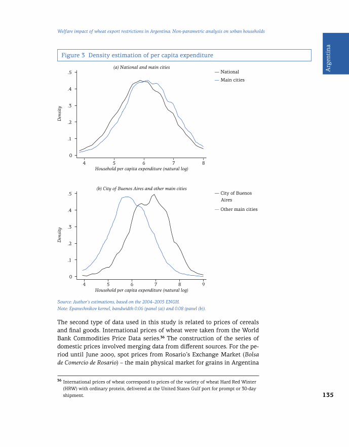
135
Arg
enti
na
Welfare impact of wheat export restrictions in Argentina: Non-parametric analysis on urban households
Figure 3 Density estimation of per capita expenditure
Source: Author’s estimations, based on the 2004–2005 ENGH.Note: Epanechnikov kernel, bandwidth 0.06 (panel (a)) and 0.08 (panel (b)).
The second type of data used in this study is related to prices of cereals and final goods. International prices of wheat were taken from the World Bank Commodities Price Data series.36 The construction of the series of domestic prices involved merging data from different sources. For the pe-riod until June 2009, spot prices from Rosario’s Exchange Market (Bolsa de Comercio de Rosario) – the main physical market for grains in Argentina
36 International prices of wheat correspond to prices of the variety of wheat Hard Red Winter (HRW) with ordinary protein, delivered at the United States Gulf port for prompt or 30-day shipment.
0
0
.2
.2
.1
.1
.3
.3
Den
sity
Den
sity
Household per capita expenditure (natural log)
Household per capita expenditure (natural log)
.5
.5
.4
.4
4
4
5
5
6
6
7
7
8
98
(a) National and main cities
(b) City of Buenos Aires and other main cities
― National
― Main cities
― City of Buenos Aires
― Other main cities

136
Trade policies, household welfare and poverty alleviation
in terms of operations and volume – were used. These prices are report-ed voluntarily by buyers and sellers; their use is not compulsory but in-dicative. However, due to interventions in the wheat market, publication of these prices was interrupted in June 2009. From July 2009 onward, first position prices (for prompt delivery) in the Futures Exchange Market of Buenos Aires were therefore used.37 Prices expressed in USD were convert-ed into ARS using the monthly nominal exchange rate published by the Central Bank of Argentina.
Finally, the series of the consumer price index was built by merging data from two sources. Disaggregated data from INDEC were used for the peri-od January 1994 to December 2006.38 From January 2007 onward, the CPI series was extrapolated using the monthly inflation rate calculated by the provincial Institute of Statistics of Santa Fe for each category of products.39 Data on money supply were obtained from the Central Bank of Argentina, and data on wage and employment from the Observatory of Employment and Entrepreneurship Dynamics and the Ministry of Labour, Employment and Social Security.
4.2 Methodology
The methodology contains three steps. The first step is to run non-para-metric regressions of the share of wheat-based products on the logarithm of expenditure per capita. In the second step, a counterfactual scenario of domestic prices that would prevail in the absence of restrictions is con-structed. This scenario is based on the key assumption of perfect pass-through from international prices (adjusted by export duties) to domestic prices in the absence of restrictions. Data on the pre-intervention period were used to test the accuracy of this assumption. The third step is to es-timate the pass-through from prices of grain to prices of its derivatives as wheat is not directly consumed by households. Coefficients were obtained for 1994–2005 when export restrictions and price controls were not yet in
37 As the interest lies in the price level and not only in price variations, current prices in the Buenos Aires Futures Exchange Market from July 2009 to December 2011 were used to continue the series. Rosario’s Exchange Market price series using the growth rate of prices on the Futures Market from July 2009 onward have not been extrapolated. To test the validity of this procedure, both series have been plotted together for 1995–2009. Except for a short period between 2002 and 2003, both markets exhibit an equal trend and levels. 38 There was a methodological change in the computation of the CPI in October 2000, which changed the base year from 1988=100 to 1999=100 and modified some criteria for the calculation. 39 This approach was adopted due to controversies that aroused in 2007 regarding data published by INDEC. In particular, there has been a debate about the official figures used to measure inflation rates during the last six years.

137
Arg
enti
na
Welfare impact of wheat export restrictions in Argentina: Non-parametric analysis on urban households
place. Using the results of these regressions, different frameworks were built, comparing the real scenario with the counterfactual one. The assess-ment of these frameworks may provide a benchmark for policy evaluation, through the calculation of welfare gains or losses for consumers generat-ed by the interventions.
Step 1: Non-parametric estimations of the share of wheat-based products in per capita household expenditure
Figure 4, panels (a) and (b), show the results of the first step of the meth-odological approach. Following Deaton (1989a, 1989b) and Benjamin and Deaton (1993), non-parametric regressions of the budget shares spent both on food and wheat-based products along the distribution of total per capita expenditure of households were estimated. This was intended to assess the importance of wheat derivatives in total expenditure. The main advantage of the use of non-parametric techniques is that it eliminates the need to formulate further assumptions about the data-generating process. These regressions represent a weighted average of the values of the food shares along the expenditure distribution and can be expressed as follows:
E m
pi qi x (1) Variables in equation (1) are defined as in Section 4.1. Since the last wave of the ENGH was conducted in 2004–2005, it is assumed that budget shares calculated from this source remained largely unchanged for the period of analysis (2006–2011).40
40 The validity of this assumption relies on several considerations. The first consideration is the absence of changes in the distribution of per capita expenditure between 2004 and 2005 and the period of analysis, 2006–2011. The second is that this assumption is more likely to hold if both the inflation rate between different groups of products and real income are constant. The third consideration is that it relies on the non-existence of changes in preferences of households. The lack of data on the per capita expenditure distribution and household preferences precludes a complete assessment. One proxy would be to analyse changes in the per capita income distribution of households. A comparison of the ratio of the income share between the highest and the lowest deciles between 2005 and 2011 is indicative of changes in the income distribution, biased towards a reduction in inequality. According to the Permanent Household Survey (Encuesta Permanente de Hogares) conducted by INDEC, this ratio was 11.4:1 in the second quarter of 2005 and 7.2:1 in the fourth quarter of 2011. Also, from December 2005 to December 2011, the accumulated inflation in Food and Beverages (196 per cent) was lower than in Bread, Cereals and Pasta (206 per cent), which could have generated a substitution of products within the Food and Beverages group, especially among the poorest households, which are more budget constrained. Both elements suggest that budget shares of the poorest households dedicated to wheat-based products could have been reduced between 2004–2005 and 2006– 2011. If this were the case, results of the policies would be less pro-poor biased, reinforcing the results of this study associated with the inefficiency of policies to avoid welfare losses for households.

138
Trade policies, household welfare and poverty alleviation
As shown in Figure 4, non-parametric regressions confirm that the poorest households spend a large share of total expenditure on food, and particu-larly basic goods such as bread and pasta, the demand for which is more inelastic to variations in prices. Therefore, changes in prices of consump-tion goods have a greater impact on the poorest households. Some differ-ences between the City of Buenos Aires and other main cities appear in Figure 4, panel (a). When the expenditure distributions overlap, the poor-est households in the City of Buenos Aires spend a lower share of total ex-penditure on food than households with the same level of per capita total expenditure located in other main cities. However, these differences disap-pear as we move to the right of the distribution. Figure 4, panel (b), shows a different pattern than panel (a). For those segments for which the ex-penditure per capita distribution overlaps, the share of total expenditure spent on wheat derivatives is similar for the City of Buenos Aires and for the other main cities.
Figure 4 Share of food and wheat-based products in total household expenditure
Source: Author’s estimations, based on the 2004–2005 ENGH.Note: Epanechnikov kernel, bandwidth 0.02, degree 1.
Step 2: Counterfactual scenario for domestic wheat prices
The construction of the counterfactual scenario accounts for the price var-iation of cereal prices that would prevail in the domestic market in the absence of quantitative export restrictions. If NTMs were not in place, do-mestic prices should follow the evolution of international prices adjust-ed by export duties, calculated as IntPrice * (1 – export duties). The main assumption is that without quantitative export restrictions in the wheat market, there would be a perfect pass-through from international prices (adjusted by export duties) to domestic prices. Consequently, changes in
0 0
.2
.1
.3
.05
Shar
e of
food
Shar
e of
bre
ad, c
erea
ls a
nd p
asta
Household per capita expenditure(natural log)
Household per capita expenditure(natural log)
.6 .2
.5.15
.4
.1
4 45 56 67 798 98
(a) Food (b) Bread, cereals and pasta― City of Buenos Aires
― Other main cities

139
Arg
enti
na
Welfare impact of wheat export restrictions in Argentina: Non-parametric analysis on urban households
adjusted international prices would be a good proxy for changes in domes-tic prices in the absence of NTMs.41 To test this assumption, ordinary least squares (OLS) regressions of the logarithm of domestic prices on the log-arithm of adjusted international prices were run.
The estimation of the elasticity of domestic wheat prices to adjusted inter-national prices for the pre-intervention period (1994–2005) and the post-in-tervention period (2006–2011) is based on equation (2).42 In this equation, the dependent variable is ln (DPW)my, the logarithm of the domestic price of wheat. ln (AdjIntPW)my is the logarithm of international prices adjusted by export duties. Prices are expressed in ARS, on a monthly basis. δ cap-tures yearly-fixed effects to take into account any year-specific factor that could affect the pass-through. Monthly-fixed effects expressed by γ capture any seasonal effect affecting this market across the year.
ln (DPW)my = β0 + β1 ln (AdjIntPW)my+ δy + γm + μmy (2)
Before presenting the results of the regression, supportive evidence for the assumption of perfect pass-through in the absence of export restrictions is discussed in Table 2 and Figure 5. This evidence also confirms that the relationship between international and domestic prices changes after the implementation of quantitative restrictions, testifying to the efficiency of the policy in reaching its main goal of disconnecting domestic wheat pric-es from international prices. The fulfillment of this goal is fundamental to justify the construction of a counterfactual scenario.
Panel (a) in Table 2 shows the share of international prices received by wheat producers, calculated as the ratio of domestic prices to internation-al prices.43 Panel (b) shows the share of international prices adjusted by export duties received by domestic wheat producers, computed as the ra-tio of domestic prices to international prices adjusted by export duties. For
41 In 1995–2011, Argentine wheat FOB prices were at 98.2 per cent of international prices. This supports the hypothesis of international prices being a good proxy for domestic prices when tariff measures and non-tariff measures are not in place. 42 See Annex 2 for a discussion related to the consistency of the OLS estimators presented in Table 3. 43 Ghezán et al. (2001) made a similar analysis comparing the decade of the 1990s with the decade of the 1980s. During 1994–1996, the share of international prices received by producers was 94 per cent and 93 per cent for wheat and corn, respectively. However, these shares had been only 66 per cent and 72 per cent during 1983–1985. This was explained both by the export duties applied to these cereals during the 1980s and by the difference between the official exchange rate and the actual prevailing exchange rate. Both measures were removed in the 1990s, which could explain the reduction in the gap between national and international prices at that time.

140
Trade policies, household welfare and poverty alleviation
1994–2001, when neither quantitative restrictions nor export duties were implemented, the share of international prices received by wheat produc-ers averaged 90 per cent. The implementation of export duties in 2002 reduced the share received by producers to an average of 71 per cent for 2002–2005. However, once international prices are adjusted by export du-ties, these shares do not differ considerably from 1994–2001 (88 per cent in panel (b)). This suggests that the implementation of these duties reduced domestic prices only by the amount of the export duties, without gener-ating additional distortions. The share of adjusted international prices re-ceived by producers declined sharply during 2006–2011 (to 59 per cent in panel (a) and 77 per cent in panel (b)).44 Quantitative export restrictions reduced competition between millers and exporters, forcing producers to sell cereals at low prices to domestic mills. Hence, the implementation of quantitative restrictions could explain the emergence of additional distor-tions besides export duties in the cereals market, stemming from increased market power of domestic millers that allowed them to push domestic wheat prices down.45
44 The gap between international and domestic prices of wheat was particularly high in the years 2008 and 2011, when the share of adjusted international prices received by producers averaged 71 per cent. 45 Competition between millers and exporters was reduced because exporters were not able to sell abroad unless they managed to get an export licence. Exporters also offered low prices to domestic producers, arguing that they were compelled to store the grain until they could manage to get an export licence and that they could not anticipate the evolution of international prices. Producers could not actually know whether exporters had a licence and were forced to sell at low prices. In many cases, they were not able to store the grain and wait for convenient prices as they had to reimburse credits related to the current harvest.
Table 2 Share of international prices received by domestic producers (per cent)
(a) International prices
Wheat Corn
1994–2001 90 95
2002–2005 71 74
2006–2011 59 65
(b) Adjusted international prices
Wheat Corn
1994–2001 90 95
2002–2005 88 91
2006–2011 77 83
Source: Author’s calculations, based on data from the World Bank, Rosario’s Exchange Market and the Buenos Aires Futures Exchange Market.

141
Arg
enti
na
Welfare impact of wheat export restrictions in Argentina: Non-parametric analysis on urban households
46 Figure A1.1 in Annex 1 presents the evolution of international prices and domestic prices not adjusted for export duties. These results reaffirm evidence from Figure A1.1 and Table 2. For 2002–2005, the price gap ((IntPrice – DomesticPrice)/IntPrice) is lower than for the post-intervention period 2006–2011. 47 Similar results are obtained using the first position prices (for prompt delivery) of wheat in the futures exchange markets of Chicago and Argentina.
During the same period, corn also faced quantitative export restrictions that were timed similarly to wheat export restrictions. The share of in-ternational prices received by corn producers is also reported in Table 2, suggesting that both markets showed similar patterns in the share of in-ternational prices received by domestic producers. This helps to rule out the possibility that changes in the share of international prices received by wheat producers during 2006–2011 were associated with other circum-stances particularly affecting the wheat market rather than with export restrictions.
Figure 5 shows monthly prices of wheat in the international and domes-tic markets (adjusted by export duties)46 for 1994–2011. As can be seen, the evolution of domestic prices is in line with the evolution of international prices for the pre-intervention period. Even after the implementation of ex-port duties (period 2002–2005), the price gap ((AdjIntPrice – DomesticPrice)/AdjIntPrice) is similar to 1994–2001 and lower than for the post-interven-tion period 2006–2011.47 In line with results presented in Table 2, Figure 5 shows that the gap between international and domestic prices increased during 2006–2011, even after controlling for export duties. This suggests that the existing price gap is measuring distortions associated with the implementation of quantitative export restrictions implemented in 2006–2011, which allowed domestic millers and exporters to exercise market power and reduce domestic prices.

142
Trade policies, household welfare and poverty alleviation
Figure 5 Evolution of international and domestic prices of wheat, 1994–2011 (USD per metric ton)
Table 3 Pass-through from international to domestic prices during pre- and post- intervention periods
Source: Author’s calculations, based on data from the World Bank, Rosario’s Exchange Market, Buenos Aires Futures Exchange Market, and Central Bank of Argentina. Note: Prices are expressed in nominal terms. International prices of wheat are adjusted by export duties.
Results of the estimations of equation (2) are presented in Table 3. These results show how changes in international prices are transmitted to do-mestic prices and hence how sensitive producers are to international prices. Pre-intervention elasticity (columns 1–3) is higher than the post-in-tervention elasticity (columns 4–6), as expected. These results may be re-flecting the implementation of export restrictions that force producers to sell in the domestic market at low prices, making it impossible for them to take full advantage of price increases in the international market. These results hold when Export Duties Wmy are included in the estimations (see Table A1.2 in Annex 1).
(1) (2) (3) (4) (5) (6)
lnDPW - PRE
lnDPW - PRE
lnDPW - PRE
lnDPW - POST
lnDPW - POST
lnDPW - POST
ln(AdjIntPW)0.99***
(0.02)1.03***
(0.07)1.09***
(0.05)0.84***
(0.06)0.72***
(0.08)0.70***
(0.07)
Constant–0.05(0.10)
–0.34(0.41)
–0.72**(0.32)
0.76*(0.39)
1.53***(0.57)
1.61***(0.50)
50
0
Jan
1994
Jan
1997
Jan
2000
Jan
2003
Jan
2006
Oct
199
4
Oct
199
7
Oct
200
0
Oct
200
3
Oct
200
6
Jul
1995
Apr
199
6
Apr
199
9
Apr
200
2
Apr
200
5
Apr
200
8
Jan
2009
Oct
200
9
Jul
2010
Apr
201
1
Jul
1998
Jul
2001
Jul
2004
Jul
2007
100
150
200
250
350
300U
SD p
er m
etri
c to
n
― International prices (ajusted by export duties)
― Domestic prices
Average price gap (2002–2005)11.7%
Average price gap (1994–2001)10.1%
Average price gap (2006–2011)22.8%

143
Arg
enti
na
Welfare impact of wheat export restrictions in Argentina: Non-parametric analysis on urban households
Source: Author’s estimations, based on data from the World Bank, Rosario’s Exchange Market and Buenos Aires Futures Exchange Market.Note: Robust standard errors in parentheses. Dependent variable: logarithm of domestic prices of wheat; *** p < 0.01, ** p < 0.05, * p < 0.1. FE stands for fixed effects.
(1) (2) (3) (4) (5) (6)
lnDPW - PRE
lnDPW - PRE
lnDPW - PRE
lnDPW - POST
lnDPW - POST
lnDPW - POST
Observations 144 144 144 72 72 72
Year FE No Yes Yes No Yes Yes
Month FE No No Yes No No Yes
R-squared 0.94 0.96 0.98 0.69 0.85 0.89
The evidence presented above confirms the hypothesis that adjusted in-ternational prices are a good proxy for domestic prices in the absence of quantitative restrictions. In particular, the results support the assumption of perfect pass-through from international to domestic prices. Therefore, the price variation in international prices of wheat is used to construct the counterfactual scenario. Moreover, regressions in Table 3 reinforce the hy-pothesis of changes in the relationship between international and domes-tic prices after the implementation of NTMs to exports. The hypothesis of equal trends and intercepts between the pre-intervention and post-inter-vention period can be rejected at 1 per cent confidence level.
Step 3: Pass-through estimations from wheat prices to final goods prices
Wheat plays only an indirect role in influencing consumer welfare through changes in the prices of its derivatives. The third methodological step con-sists of the estimation of the pass-through from wheat prices to prices of wheat-based products. Results of the estimations are used to calculate the share of the total variation in cereal prices that is actually perceived by con-sumers through changes of prices of basic consumption goods. Estimations are based on equation (3). ln (CPIBCP)my is the logarithm of the monthly CPI of Bread, Cereals and Pasta, ln (DPW)my stands for the logarithm of monthly average domestic prices of wheat expressed in ARS and Xmy is a set of con-trols that includes different ways of capturing inflation. Among them, the logarithm of the CPI of other groups of products is included,48 as well as the logarithm of the monetary base or money supply and the average wage of formal workers in different activities.49 The nominal exchange rate, the
48 The selection criterion was to choose sectors that seem less likely to be the target of government interventions aiming to contain inflation or implemented due to social reasons, such as Apparel and Recreation. 49 These activities include food production, milling industry, production of bakery products and pasta, according to the International Standard Industrial Classification at 4 digits.

144
Trade policies, household welfare and poverty alleviation
annual GDP at constant prices and a dummy variable POST, which equals 1 after January 2002, are included in different specifications. As in equation (2), yearly- (δy) and monthly-fixed effects (γm) are used:
ln (CPIBCP)my = β1 ln (DPW)my + Xmy + δy + γm + μmy (3)
Table 4 presents OLS estimations for different specifications of equation (3) for the pre-intervention period (1994–2005). The coefficient of interest, β1, reflects the relationship between the logarithm of wheat price in the do-mestic market and the logarithm of wheat-based products CPI, the depend-ent variable. As additional controls, column (1) includes the logarithm of CPI of other groups of products to capture inflation, the logarithm of an-nual GDP and the nominal exchange rate. β1 is positive and significant at 1 per cent confidence level. Specification (2) adds yearly- and monthly-fixed effects.50 As additional controls, column (3) includes the logarithm of mon-ey supply (M3) and the logarithm of wages of formal workers in the bak-ery industry.51 Neither of those variables enters significantly in regression (3). Specification (4) adds the money supply and the wages of formal work-ers lagged one and two periods. Only wages lagged two periods are posi-tive and significant at 5 per cent. In all cases, the sign and significance of β1 remain constant,52 although smaller in magnitude. As a robustness check, column (5) replicates column (3) for the fresh bread CPI. The coefficient as-sociated with the wheat price is still positive and significant at 1 per cent and with a higher magnitude than in previous specifications.
50 Yearly-fixed effects are included to account for potential factors such as weather conditions, changes in the labour market or any other year-specific factors affecting the pass-through from wheat to Bread, Cereals and Pasta in a particular year. Monthly-fixed effects are included to account for potential seasonality in the relationship between variables. 51 Data on this variable are only available from January 1995. 52 This result is robust to multiple specifications not reported in Table 5, such as using lagged values of the logarithm of domestic prices of wheat or using a single measure of inflation (excluding either Recreation or Apparel CPI). Also, the effect of wheat prices on Bread, Cereals and Pasta CPI holds when different variables to measure wages, different monetary variables (as M2 or monetary base) or lagged values of these variables are included. Results are robust to the change of the time period to 1994–2001. Finally, results do not change when regressions are run without a constant (see Table A1.4 in Annex 1).
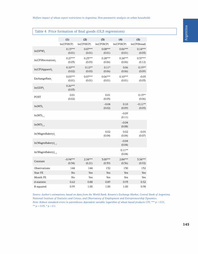
145
Arg
enti
na
Welfare impact of wheat export restrictions in Argentina: Non-parametric analysis on urban households
Table 4 Price formation of final goods (OLS regressions)
(1) (2) (3) (4) (5)
ln(CPIBCP) ln(CPIBCP) ln(CPIBCP) ln(CPIBCP) ln(CPIBread)
ln(DPW)t
0.13***(0.01)
0.07***(0.01)
0.08***(0.01)
0.06***(0.01)
0.14***(0.03)
ln(CPIRecreation)t
0.27***(0.03)
0.23***(0.05)
0.28***(0.06)
0.24***(0.06)
0.37***(0.12)
ln(CPIApparel)t
0.10***(0.02)
0.12**(0.05)
0.11*(0.06)
0.06(0.06)
0.19**(0.09)
ExchangeRatet
0.05***(0.01)
0.07***(0.01)
0.06***(0.01)
0.10***(0.01)
-0.03(0.03)
ln(GDP)t
0.26***(0.03)
POST0.01
(0.02)0.01
(0.03)0.13**(0.06)
ln(M3)t
–0.04(0.02)
0.10(0.09)
–0.11**(0.05)
ln(M3)t–1
–0.09(0.11)
ln(M3)t–2
–0.04(0.08)
ln(WagesBakery)t
0.02(0.04)
0.02(0.04)
–0.05(0.07)
ln(WagesBakery)t–1
–0.04(0.04)
ln(WagesBakery)t–2
0.11**(0.04)
Constant–0.94***
(0.34)2.54***
(0.21)3.00***
(0.39)2.84***
(0.36)3.54***
(0.92)
Observations 144 144 132 130 132
Year FE No Yes Yes Yes Yes
Month FE No Yes Yes Yes Yes
d-statistic 0.62 0.88 0.89 0.93 0.52
R-squared 0.99 1.00 1.00 1.00 0.98
Source: Author’s estimations, based on data from the World Bank, Rosario’s Exchange Market, Central Bank of Argentina, National Institute of Statistics and Census, and Observatory of Employment and Entrepreneurship Dynamics.Note: Robust standard errors in parentheses; dependent variable: logarithm of wheat-based products CPI; *** p < 0.01, ** p < 0.05, * p < 0.1.

146
Trade policies, household welfare and poverty alleviation
Coefficients from Table 4, reflecting the pass-through from wheat pric-es to consumer prices, are far below 1. Because cereals represent only a small share of bread production costs, this result should not be surprising. Different studies presented by the Argentine Rural Confederation (CRA) in their monthly seminars titled “From land to the table”53 highlight a low-er incidence of producer prices of wheat on consumer prices of derivative goods in Argentina, compared with those in other countries such as the United States or New Zealand. According to CRA estimations, the share of wheat in bread price is only about 8 per cent. The remaining share of bread price is explained by other cost elements such as utilities, freights, wages, rents and taxes. Beibe et al. (2010) find that wheat explains only about 12 per cent of bread prices. Results in Table 4 are coherent with these findings and relevant in economic terms. An increase of 10 per cent in the price of wheat is associated with an increase ranging from 0.6 to 1.3 per cent in the price of derivatives. The incidence on consumer prices of changes in the wheat price is proportional to the share of the final good price that is ex-plained by the primary input.54
When the different specifications of equation (3) are run for the post-inter-vention period (not reported), the coefficient of interest appears negative and not statistically different from zero. This could be reflecting a change in the elasticity of wheat-based product prices to wheat prices during the post-intervention period. If that were the case, then using the coefficients from Table 4 to calculate the price increase of final goods that could be at-tributed to wheat during the post-intervention period could be misleading. However, the change in magnitude and significance of β1 could be better explained by the interventions in the wheat market. As already mentioned, the price of wheat effectively paid by the mill that ultimately affects con-sumers is the internal supply price set by law in 2007 and kept at an ar-tificially low level during 2007–2011. The large gap between the internal supply price and the domestic price (see Figure 1) explains why domestic prices are not statistically significantly related to the CPI of wheat-based products for the post-intervention period.
To sum up, the share of wheat-based products in household expenditure and the estimation of price elasticity from wheat prices to final goods pric-es were presented in this section. These results will be used to estimate the welfare effect on households of wheat export restrictions compared with a
53 In Spanish, “De la tierra a la mesa”. 54 The analysis based on the unit root test and co-integration confirms the validity of the coefficients (see Annex 2). A pass-through of 8 per cent will be assumed in the welfare analysis presented in the next section.
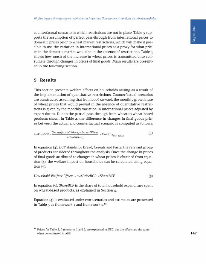
147
Arg
enti
na
Welfare impact of wheat export restrictions in Argentina: Non-parametric analysis on urban households
55 Prices for Table 5, frameworks 1 and 2, are expressed in USD, but the effects are the same when denominated in ARS.
counterfactual scenario in which restrictions are not in place. Table 3 sup-ports the assumption of perfect pass-through from international prices to domestic prices prior to wheat market restrictions, which will make it pos-sible to use the variation in international prices as a proxy for what pric-es in the domestic market would be in the absence of restrictions. Table 4 shows how much of the increase in wheat prices is transmitted onto con-sumers through changes in prices of final goods. Main results are present-ed in the following section.
5 Results
This section presents welfare effects on households arising as a result of the implementation of quantitative restrictions. Counterfactual scenarios are constructed assuming that from 2006 onward, the monthly growth rate of wheat prices that would prevail in the absence of quantitative restric-tions is given by the monthly variation in international prices adjusted by export duties. Due to the partial pass-through from wheat to wheat-based products shown in Table 4, the difference in changes in final goods pric-es between the actual and counterfactual scenario is computed as follows:
%∆PriceBCP = Counterfactual Wheatt – Actual Wheatt
* ElasticityBCP, Wheat
(4)
―――――――――――――――――――
ActualWheatt
In equation (4), BCP stands for Bread, Cereals and Pasta, the relevant group of products considered throughout the analysis. Once the change in prices of final goods attributed to changes in wheat prices is obtained from equa-tion (4), the welfare impact on households can be calculated using equa-tion (5):
Household Welfare Effects = %∆PriceBCP * ShareBCP (5)
In equation (5), ShareBCP is the share of total household expenditure spent on wheat-based products, as explained in Section 4.
Equation (4) is evaluated under two scenarios and estimates are presented in Table 5 as framework 1 and framework 2.55

148
Trade policies, household welfare and poverty alleviation
Framework 1 evaluates the effect of quantitative restrictions on prices of wheat-based products. It compares actual prices of wheat in the do-mestic market with counterfactual prices,56 which are built under the assumption that in the absence of restrictions, the price variation in inter-national markets is a good proxy for price changes in the domestic market. Counterfactual price data are built from January 2006. While domestic wheat prices increased by 64 per cent from 2005 to 2011, counterfactual prices would have increased by 84 per cent for the same period, thus mak-ing the average price of wheat 12.4 per cent higher in 2011. According to the estimations in Table 4, only about 8 per cent of the change in wheat prices is actually transmitted to final goods and thus has an effect on con-sumers. So, as per equation (4), in the absence of quantitative restrictions, the increase in prices of wheat-based products generated by changes in wheat prices would be 1 per cent higher than in the real scenario. Figure 6, panel (a) shows that consumer welfare effects generated under frame-work 1 are negligible. The sole adoption of quantitative export restrictions was not enough to produce a quantifiable effect on the welfare of urban households. If the restrictions were removed, for the City of Buenos Aires,
Table 5 Estimations of price variation of wheat-based products
Actual Counterfactual
Framework 1 Domestic wheat prices
2005 100.1 100.1
2011 164.0 184.4
Growth (2005-2011) 64% 84%
Difference in wheat prices 12.4%
%∆PriceBCP 1.0%
Framework 2 Internal supply prices
2005 100.1 100.1
2011 102.3 184.4
Growth (2005-2011) 2% 84%
Difference in wheat prices 80.2%
%∆PriceBCP 6.4%
Source: Author’s estimations, based on data from the World Bank, Rosario’s Exchange Market, Buenos Aires Futures Exchange Market, Central Bank of Argentina, INDEC, and Statistics Institute of Santa Fe.Note: Domestic and internal supply prices are calculated as annual averages.
56 Counterfactual scenarios in Table 5 were constructed extrapolating domestic prices of wheat since January 2006, using the variations in international prices adjusted by export taxes, as was previously explained. Alternative scenarios reported in Annex 3 rely on alternative assumptions to build counterfactual scenarios. Results do not differ systematically from the case presented in the main body of the study.

149
Arg
enti
na
Welfare impact of wheat export restrictions in Argentina: Non-parametric analysis on urban households
Figure 6 Potential welfare effects on urban households
Source: Author’s estimations, based on the 2004–2005 ENGH.Note: Epanechnikov kernel, bandwidth 0.2, degree 1.
all households would suffer welfare losses lower than 0.1 per cent. For oth-er main cities, only the poorest decile of the per capita distribution would experience welfare losses higher than 0.1 per cent, but not exceeding 0.2 per cent in any case.
Framework 2 jointly evaluates the effect of quantitative bans and ceiling prices artificially set at lower levels than domestic prices. To take account of the effects of both policies, framework 2 uses internal supply prices as a measure of actual prices of wheat. This assumption is justifiable because it is the internal supply price that ultimately determines the prices of final goods and hence affects consumers. Framework 2 in Table 5 shows that, in this case, prices of wheat-based products would be 6.4 per cent higher in the counterfactual scenario than in the real scenario. Non-parametric estimations of welfare effects of framework 2 are shown in Figure 6, pan-el (b). If neither export restrictions nor internal supply prices were imple-mented, urban households in the main cities would suffer welfare losses ranging from zero to almost 1.5 per cent compared with the real scenar-io. These effects are very modest for most households, even though the poorest households are the most affected, reflecting the pro-poor bias of the measures. For main cities other than the City of Buenos Aires, only the lowest quartile of the logarithm of the expenditure per capita distri-bution would suffer welfare losses higher than 0.5 per cent if the policies were removed. Welfare losses would be higher than 1 per cent only for the lowest percentile of the distribution. These effects would be even more modest for households located in the City of Buenos Aires, where welfare losses never exceed 0.5 per cent and are actually close to zero for the rich-est households.
-.002 -.015
Wel
fare
cha
nge
Wel
fare
cha
nge
Household per capita expenditure(natural log)
Household per capita expenditure(natural log)
0 0
-.0005-.005
-.0015
-.001
-.01
4 45 56 67 79 98 8
(a) Framework 1 (b) Framework 2― City of Buenos Aires
― Other main cities

150
Trade policies, household welfare and poverty alleviation
Together, results from frameworks 1 and 2 indicate that the implementa-tion of wheat export restrictions alone does not seem to have generated quantifiable effects on consumers. When combined with ceiling prices and subsidies to the milling industry, welfare effects on households do appear, but are small in magnitude.
5.1 Effects of the macroeconomic context on final goods prices
Were the policies implemented in the wheat market sufficient to curb in-flation in basic goods? What would be the evolution of prices of wheat-based products in the absence of interventions? It would be expected that lower actual domestic prices of wheat compared to counterfactual prices (see Table 5) would result in lower prices of final goods. High inflation in wheat-based products during 2006–2011 could have been even higher with counterfactual prices of wheat.
To address this concern, the coefficients from Table 4, column (2), are used to linearly predict the prices of wheat-based products that would prevail in the domestic market with counterfactual prices of wheat (i.e. in the absence of interventions in the wheat market). Counterfactual prices of wheat used for these linear predictions are the same as those used for the construction of frameworks 1 and 2. It is important to remember that co-efficients in Table 4 were obtained for 1994–2005, and when using them to predict prices for 2006–2011, it should be assumed that price formation mechanisms were kept constant between periods.
Actual consumer price indices in Table 6 are the average CPI of the Bread, Cereals and Pasta group for 2005 and 2011. The counterfactual CPI for 2011 is obtained from the linear prediction explained in the paragraph above.57
Table 6 Consumer price index of wheat-based products
Actual Counterfactual
2005 154.5 154.5
2011 440.2 261.1
Growth CPI (2005–2011) 185% 69%
Difference in CPI –40.70%
Source: Author’s estimations, based on data from INDEC and Statistics Institute of Santa Fe, and author’s calculations presented in Table 4.Note: Actual and counterfactual CPI of Bread, Cereals and Pasta for 2005 and 2011 are constructed as annual averages.
151
Arg
enti
na
Welfare impact of wheat export restrictions in Argentina: Non-parametric analysis on urban households
The counterfactual estimation in Table 6 does not allow for disentangling the effect of export restrictions from the remaining policies and macroe-conomic conditions affecting Argentina in the last years. If the boom of in-ternational commodity prices were the main source behind domestic food inflation, it should be expected that predicted prices of wheat derivatives, estimated with counterfactual wheat prices (higher than domestics pric-es), would be higher than actual prices. However, while actual inflation in wheat-based products was 185 per cent between 2005 and 2011, inflation in the counterfactual scenario would only have been 69 per cent during the same period. According to the estimations in Table 6, prices of final goods would be 40.7 per cent lower with counterfactual prices of wheat.
The inefficiency of lower wheat prices in restraining inflation can be relat-ed to the minor role that wheat plays in the price formation of wheat-based products, as already discussed. Potential explanations for the increase in prices of wheat derivatives during 2006–2011 should be sought beyond the increase in wheat prices in international markets. Moreover, these results could reflect a change in the price formation mechanism of final goods.58 Other causes might have spurred inflation in 2006–2011, or even the same cause might have played a different role. In this case, coefficients obtained in Table 4 for the pre-intervention period may not be a good fit to predict prices of final goods in the post-intervention period.
To sum up, the frameworks presented in Table 5 shed light on the idea that export restrictions by themselves were not enough to generate quantifia-ble welfare effects on consumers. Framework 1 shows that in the absence of export restrictions, domestic prices of wheat would only be 12.4 per cent higher than in the real scenario, causing a negligible impact on consum-er welfare. Also, when ceiling prices and subsidies to millers are consid-ered, a small impact on household welfare appears, as can be concluded based on framework 2. In this framework, counterfactual prices of wheat would be 80 per cent higher than real prices, making wheat-based prod-uct prices 6.4 per cent higher than in the real scenario. Because the share of wheat in final goods prices is about 8 per cent in estimations in Table 4, and the share of wheat-based products in total household expenditure is never higher than 20 per cent, the intervention in the wheat market does not seem to have generated a measurable effect on household welfare.
57 The counterfactual CPI for 2005 is the same as the actual CPI, since the counterfactual scenario were only estimated from 2006 onward. 58 For example, in the post-intervention period, the inflationary environment may have played a higher role in pushing the prices of wheat-based products up than in the pre-intervention period. Between 2005 and 2011, the accumulated general inflation was 156 per cent, while in the pre-intervention period (1994–2005) the accumulated inflation was 78 per cent, supporting the idea of changes in the inflationary environment.
152
Trade policies, household welfare and poverty alleviation
Evidence obtained so far supports the idea that policies applied to the wheat market fell short of the expected goals of the government. As sug-gested above, the increase in prices of final goods may have been even higher in the absence of interventions. However, high prices of wheat in international markets should not be blamed for the price spike in domes-tic prices of wheat-based products. Even if export restrictions helped to re-duce the share of the price increase of final goods attributable to wheat prices, most of the increase in wheat-based product prices was not avoid-able. Other price components of wheat-based products may have played a major role.
6 Conclusions
Studies addressing the effects of non-tariff measures are far from abun-dant. In this sense, this study presents one of the first attempts to evalu-ate the largely unexplored effects of this kind of trade policy in Argentina.
The implementation of quantitative export restrictions on cereals trig-gered an intense debate in Argentina between supporters and opponents of these measures. For supporters, the justification behind the implemen-tation of export restrictions was twofold. First, in a situation character-ized by high international prices of commodities, this policy intended to detach domestic from international prices and thus avoid a large increase in domestic prices. Since derivatives of wheat are an important compo-nent of the basic food basket of the typical Argentine household, export restrictions aimed to limit inflation. Second, the policy also aimed to keep an adequate provision of grains in the domestic market. Opponents of ex-port restrictions emphasize the minor role that wheat plays in the price formation of final goods. If other components of final goods prices are not targeted, controlling the prices of primary inputs would not be enough to curb inflation.
Additionally, in the medium term, export restrictions could potentially affect incentives on the production side, reduce the supply of cereals in the domestic market and thus increase domestic prices. Debates around wheat export restrictions intensified in the early months of 2013, due to the spike in prices of wheat, flour and bread in the Argentine domestic mar-ket (Bertello, 2013; Koop, 2013). This recent increase in prices can be asso-ciated with a shortage of wheat for use in local industry, which led to the adoption of additional measures in this market.59
59 See Bureau of Domestic Trade, Resolution 67/2013.

153
Arg
enti
na
Welfare impact of wheat export restrictions in Argentina: Non-parametric analysis on urban households
A main assumption of this study is that, in the absence of interventions, domestic wheat prices would move together with international prices. Evidence supporting this assumption allowed for constructing a counter-factual scenario in which the growth rate of domestic wheat prices would equal the variation in international prices adjusted by export duties. Also, the pass-through from wheat prices to prices of final goods was estimated. Combining both results, a calculation was made of the difference in the in-crease in final goods prices which can be attributed to the difference in the increase in wheat prices between the real and the counterfactual scenario. The share of household budget spent on wheat derivatives allowed an as-sessment of the welfare effect of export restrictions on urban households, through the evaluation of two different frameworks.
Main results suggest that non-tariff measures by themselves were not enough to generate a large welfare effect on households. In the absence of export restrictions, the price increase of wheat-based products attribut-able to wheat would only be 1 per cent higher than in the real scenario, with negligible welfare effects on urban consumers. If both export restric-tions and subsidies to the milling industry were removed, prices of fi-nal goods would be 6.4 per cent higher in the counterfactual scenario. Welfare losses would be modest, ranging from zero to 1.5 per cent, main-ly affecting the poorest households. For main cities other than the City of Buenos Aires, only the lowest quartile of the distribution would suffer wel-fare losses higher than 0.5 per cent. Welfare losses higher than 1 per cent would be limited to the poorest percentile of the per capita distribution. These results testify to the inefficiency of the set of policies (quantitative export restrictions, ceiling prices and subsidies) to curb inflation and gen-erate quantifiable welfare effects on households, compared with a non-in-tervention scenario. It was only possible to limit the increase in food prices partially and at the cost of a large financial burden for the government in terms of subsidies. Additionally, export restrictions reduced the amounts collected by the government in the form of export duties, generating addi-tional costs from the intervention.
To analyse the causes of food inflation does not fall under the scope of this study. However, results suggest that key causes of inflation in wheat-based products may be sought beyond the international boom in wheat prices. The design of policies aiming to control increases in food prices should therefore go beyond targeting commodity prices in the domestic market, as other price components seem to play a more important role in push-ing the prices up.
154
Trade policies, household welfare and poverty alleviation
As was previously discussed, a comprehensive analysis should incorporate the effects of NTMs on other actors involved in the wheat value chain than consumers. In particular, producer welfare effects should be addressed, but the lack of available data precludes this analysis. However, some general phenomena such as the high volatility in domestic wheat prices in 201360 and the reduction of wheat-sown areas could be indicative of the distortion of the incentives faced by wheat producers as a consequence of the poli-cies implemented in the wheat sector. In addition, interventions may also have generated large gains for a limited group of millers and exporters re-ceiving subsidies and export authorizations, while placing a large financial burden on the government.
New policies implemented after 2011, such as the creation of a trust in May 2013 to refund export duties to wheat producers, were intended to promote wheat production, with the aim to counterbalance the negative incentives emanating from the implementation of export restrictions. However, ef-fects of these measures will only appear in the medium term and cannot be assessed at the moment.
Also, export restrictions may have had an impact on fostering the first and second processing stages. By providing a higher level of effective protec-tion, NTMs might have promoted national value added and employment. Figures presented in Section 2 of the study support this idea; however, ev-idence is far from being conclusive.
Overall, although limited to first-order consumption effects on urban house-holds, this study contributes to providing a benchmark to evaluate the ef-fects of the policies in motion. These policies did not seem sufficient to generate large welfare effects on consumers compared with a potential counterfactual scenario. In addition, the implementation of export restric-tions in the wheat market was not sufficient to contain inflation in wheat derivatives in Argentina from 2007 onward. These results are highly rele-vant in terms of policymaking because they seem indicative of the failure of NTMs to achieve the intended objectives. It is possible that, in the absence of interventions, the increase in prices of final goods would be even higher than it actually was. Still, it is not clear whether these welfare losses would be quantitatively larger than in the real scenario, provided that in both cas-es, households would suffer due to increases in wheat-based product prices.
60 In October 2013, international wheat prices averaged USD 325 per metric ton (World Bank Commodities Price Data). In the same month, domestic wheat prices were almost double, averaging USD 617 per metric ton (Buenos Aires Futures Exchange Market). Higher domestic prices thus reversed any potential positive effect of export restrictions on consumers.

155
Arg
enti
na
Welfare impact of wheat export restrictions in Argentina: Non-parametric analysis on urban households
Moreover, changes in domestic wheat prices could even have generated negative welfare effects on the supply side. If this had been the case, neg-ative welfare effects on producers could have offset the modest positive welfare effects on consumers. Therefore, it is possible that an alternative al-location of resources would be more beneficial from a social point of view.
To sum up, results obtained so far raise doubts about the effectiveness of export restrictions in achieving welfare goals. Future research on this top-ic should try to incorporate the supply side in the analysis, provided that microdata on producers are available. This could help assess the impact of these policies in a broader context. In addition, future analysis should as-sess medium- and long-term effects of export restrictions and other policies implemented in the wheat market. It would also be relevant to study the effects of export restrictions on other cereals, such as corn. Such analysis would help to estimate the overall impact that export-related NTMs have had on the welfare of households in Argentina as well as to better under-stand the effects of this type of policies. Finally, the effectiveness of export duties as a policy intended to curb inflation and generate welfare effects on households should also be discussed. Although the implementation of export duties was driven by fiscal considerations, it also had an effect on the prices of wheat derivatives. Also, by reducing the share of internation-al prices received by producers, incentives and choices on the supply side were distorted. However, welfare effects associated with the removal of ex-port duties were not studied here and will be left for future research.

156
Trade policies, household welfare and poverty alleviation
Annexes
Annex 1
Table A1.1 Summary statistics by quintile of the income distribution, 2004–2005
Source: Author’s estimations, based on the 2004–2005 ENGH.Note: Summary statistics are calculated at the household level. Total per capita expenditure is expressed in ARS.
1st quintile
2nd quintile
3rd quintile
4th quintile
5th quintile
National
Total per capita expenditure 169 288 420 614 1,291
Share of food in expenditure 50.9% 44.4% 39.1% 36.0% 29.1%
Share of wheat-based products in expenditure
11.0% 7.8% 6.0% 5.0% 3.3%
Equivalent adults per household 3.8 3.2 2.8 2.3 1.9
City of Buenos Aires
Total per capita expenditure 477 701 984 1,435 2,530
Share of food in expenditure 37.6% 34.4% 30.7% 27.0% 24.2%
Share of wheat-based products in expenditure
5.6% 4.4% 3.7% 2.7% 1.9%
Equivalent adults per household 2.8 2.2 2 1.8 1.6
Other main cities
Total per capita expenditure 210 331 457 628 1,167
Share of food in expenditure 47.8% 42.4% 38.8% 36.3% 29.8%
Share of wheat-based products in expenditure
9.7% 6.9% 5.7% 4.7% 3.4%
Equivalent adults per household 3.6 3 2.7 2.4 2

157
Arg
enti
na
Welfare impact of wheat export restrictions in Argentina: Non-parametric analysis on urban households
Source: Author’s estimations, based on data from the World Bank, Rosario’s Exchange Market and Buenos Aires Futures Exchange Market.Note: Robust standard errors in parentheses. Dependent variable: logarithm of domestic wheat prices; *** p < 0.01, ** p < 0.05, * p < 0.1.
Source: Author’s estimations, based on data from the World Bank, Rosario’s Exchange Market and Buenos Aires Futures Exchange Market.Note: Robust standard errors in parentheses. Dependent variable: logarithm of domestic wheat prices; *** p < 0.01, ** p < 0.05, * p < 0.1.
Table A1.2 Pass-through from international to domestic prices of wheat – Export duties as control
Table A1.3 Pass-through from international to domestic prices of wheat – Estimations of first differences
(1) (2) (3) (4) (5) (6)
lnDPW -PRE
lnDPW -PRE
lnDPW -PRE
lnDPW -POST
lnDPW -POST
lnDPW -POST
ln(AdjIntPW) 0.98***(0.06)
0.95***(0.10)
1.14***(0.10)
0.77***(0.06)
0.69***(0.09)
0.66***(0.07)
ExportDutiesW 0.00(0.00)
0.01(0.01)
-0.01(0.01)
0.02**(0.01)
0.01(0.01)
0.01**(0.01)
Constant –0.01(0.28)
0.13(0.50)
–0.85*(0.48)
0.85**(0.37)
1.46***(0.55)
1.55***(0.45)
Observations 144 144 144 72 72 72
Year FE No Yes Yes No Yes Yes
Month FE No No Yes No No Yes
R-squared 0.94 0.96 0.98 0.71 0.85 0.89
(1) (2) (3) (4) (5) (6)
lnDPW -PRE
lnDPW -PRE
lnDPW -PRE
lnDPW -POST
lnDPW -POST
lnDPW -POST
D.ln(AdjIntPW) 0.80***(0.08)
0.72***(0.10)
0.80***(0.11)
0.31**(0.13)
0.30**(0.13)
0.30**(0.11)
ExportDutiesW –0.00(0.00)
–0.00(0.00)
0.00(0.00)
–0.00(0.00)
–0.01(0.01)
–0.00(0.01)
Constant 0.00(0.01)
0.02(0.07)
–0.01(0.07)
0.11(0.09)
0.18(0.18)
0.07(0.17)
Observations 143 143 143 72 72 72
Year FE No Yes Yes No Yes Yes
Month FE No No Yes No No Yes
R-squared 0.44 0.47 0.63 0.16 0.20 0.47

158
Trade policies, household welfare and poverty alleviation
Table A1.4 Price formation of final good – Estimations without constant (OLS regressions)
(1) (2) (3) (4) (5)
ln(CPIBCP) ln(CPIBCP) ln(CPIBCP) ln(CPIBCP) ln(CPIBread)
ln(DPW)t 0.12***(0.01)
0.07***(0.01)
0.08***(0.01)
0.06***(0.01)
0.14***(0.03)
ln(CPIRecreation)t 0.33***(0.03)
0.23***(0.05)
0.28***(0.06)
0.24***(0.06)
0.37***(0.12)
ln(CPIApparel)t 0.09***(0.02)
0.12**(0.05)
0.11*(0.06)
0.06(0.06)
0.19**(0.09)
ln(GDP)t 0.16***(0.01)
0.21***(0.02)
0.24***(0.03)
0.22***(0.03)
0.30***(0.08)
ExchangeRatet 0.05***(0.01)
0.07***(0.01)
0.06***(0.01)
0.10***(0.01)
-0.03(0.03)
POST –0.01(0.02)
–0.01(0.02)
ln(M3)t –0.04(0.02)
0.10(0.09)
–0.11**(0.05)
ln(M3)t-1 –0.09(0.11)
ln(M3)t-2 –0.04(0.08)
ln(WagesBakery)t 0.02(0.04)
0.02(0.04)
–0.05(0.07)
ln(WagesBakery)t-1 –0.04(0.04)
ln(WagesBakery)t-2 0.11**(0.04)
Observations 144 144 132 130 132
Year FE No Yes Yes Yes Yes
Month FE No Yes Yes Yes Yes
R-Squared 1.00 1.00 1.00 1.00 1.00
d-statistic 0.59 0.88 0.89 0.93 0.52
Source: Author’s estimations, based on data from the World Bank, Rosario’s Exchange Market, Central Bank of Argentina, National Institute of Statistics and Census, and Observatory of Employment and Entrepreneurship Dynamics.Note: Robust standard errors in parentheses; dependent variable: logarithm of wheat-based products CPI; *** p < 0.01, ** p < 0.05, * p < 0.1.

159
Arg
enti
na
Welfare impact of wheat export restrictions in Argentina: Non-parametric analysis on urban households
Source: Author’s estimations, based on World Bank, Rosario’s Exchange Market, Buenos Aires Futures Exchange Market and Central Bank of Argentina. Note: Prices are expressed in nominal terms. International prices are not adjusted by export duties.
Figure A1.1 Evolution of international and domestic prices of wheat, 1994–2011 (USD per metric ton)
Annex 2
When working with time series, the consistency of OLS estimators is not guaranteed. To address the issue of potential spurious regressions, the ex-istence of unit roots in the time series of interest is tested. For 1994–2005, the augmented Dickey-Fuller test does not reject the null hypothesis of the existence of a unit root for the logarithm of domestic and adjusted in-ternational prices.61 However, different specifications of both the Johansen and the Engle and Granger tests reject the null hypothesis of no co-integra-tion at 1 per cent for the pre-intervention period. These results support the existence of long-term equilibrium between variables and dissipate con-cerns about the consistency of OLS estimators in Table 3. For the post-in-tervention period, the unit-root hypothesis for the logarithm of domestic and adjusted international prices can be rejected at 5 or 10 per cent, when
61 For domestic prices, when the specification includes a drift, the null hypothesis of the unit root could be rejected at 5 per cent with one lag and at 10 per cent with two lags. However, these results are not robust to the inclusion of a trend, or other number of lags.
50
0
Jan
1994
Jan
1997
Jan
2000
Jan
2003
Jan
2006
Oct
199
4
Oct
199
7
Oct
200
0
Oct
200
3
Oct
200
6
Jul
1995
Apr
199
6
Apr
199
9
Apr
200
2
Apr
200
5
Apr
200
8
Jan
2009
Oct
200
9
Jul
2010
Apr
201
1
Jul
1998
Jul
2001
Jul
2004
Jul
2007
100
150
200
250
450
350
400
300
USD
per
met
ric
ton
― International prices
― Domestic prices
Average price gap (2002–2005)28.7%
Averge export duties 19%
Average price gap (1994–2001)10.1%
Averge export duties 0%
Average price gap (2006–2011)40.6%
Averge export duties 23%
160
Trade policies, household welfare and poverty alleviation
the Dickey-Fuller test is performed, including a drift. These results are ro-bust to the inclusion of different numbers of lags. Thus, results of Table 3 are also consistent for the post-intervention period.62
There is also concern regarding results in Table 4 reflecting spurious re-gressions, as evidenced by low values of Durbin-Watson statistics and high R-squared. For the pre-intervention period, all the relevant series63 were found to be I(1), at standard levels of significance, including a drift and dif-ferent number of lags. The hypothesis of no co-integration cannot be re-jected when only lnCPIBCP and lnDPW are included in a Johansen test. However, the inclusion of a third variable such as GDP or a proxy for inflation (as Apparel or Recreation CPI) allows rejecting the hypothesis of no co-integration, supporting the existence of a stable long-term rela-tionship between variables. Performing the Johansen co-integration test for the whole set of relevant variables (lnCPIBCP, lnDPW, lnCPIRecreation, lnCPIApparel, lnGDP, ExchangeRate, lnM3 and lnBakeryWages) allows for the rejection of the no co-integration hypothesis. Results are robust to the in-clusion of different number of lags and different combinations of variables. These results mitigate the concern regarding results in Table 4 being driv-en by spurious relations between variables.
Annex 3
In Section 5, different frameworks of welfare effects on urban households in the City of Buenos Aires and other main cities were reported. The coun-terfactual scenario assumed in that case was constructed considering that, from January 2006 onward, the growth rate of domestic wheat pric-es would be equal to the growth rate of international prices adjusted by export duties. Tables A3.1 and A3.2 in this Annex present the same frame-works as those found in Table 5 of Section 5, but consider different assump-tions in the construction of counterfactual scenarios.
Frameworks 1A and 2A assume that in the absence of quantitative restric-tions counterfactual prices would be the international prices adjusted by
62 To avoid additional concern about the potential spurious regressions in Table 3, Table A1.3 presents the same regressions as Table 3 but with variables expressed in first differences. Because variables are found to be I(1), first differences of these variables are stationary. Results are supportive of a higher impact of international prices on domestic prices for the pre-intervention period. 63 These series are the logarithm of Bread, Cereals and Pasta CPI, the logarithm of Recreation and Apparel CPI, the logarithm of the monetary base and money supply and the logarithm of wages in the bakery and milling industries.

161
Arg
enti
na
Welfare impact of wheat export restrictions in Argentina: Non-parametric analysis on urban households
export duties. Table A3.1 reports the corresponding prices and growth rates. If only quantitative restrictions were considered, prices of wheat in the counterfactual scenario would be 48.5 per cent higher than in the real scenario. Wheat-based product prices, ascribable to wheat, would be 3.9 per cent higher in the counterfactual scenario. If internal supply pric-es were also considered, price variation in wheat-based products attributa-ble to wheat would reach 11 per cent. As can be seen in Figure A3.1, if this counterfactual scenario were assumed, interventions would avoid larger welfare losses than those estimated in the frameworks presented in Table 5. Even though, without the implementation of internal supply prices, ex-port restrictions by themselves would not seem to generate quantifiable welfare effects, as shown in Figure A3.1, panel (a).
Actual Counterfactual
Framework 1 Domestic wheat prices
2005 100.1 100.1
2011 164.0 243.5
Growth (2005-2011) 64% 143%
Difference in wheat prices 48.5%
%∆PriceBCP 3.9%
Framework 2 Internal supply prices
2005 100.1 100.1
2011 102.3 243.5
Growth (2005-2011) 2% 143%
Difference in wheat prices 138%
%∆PriceBCP 11%
Table A3.1 Estimations of price variation of wheat-based products – Alternative counterfactual scenarios A
Source: Author’s estimations, based on data from the World Bank, Rosario’s Exchange Market, Buenos Aires Futures Exchange Market, Central Bank of Argentina, INDEC, and Statistics Institute of Santa Fe. Note: Domestic and internal supply prices are calculated as annual averages. Counterfactual prices of wheat are calculated as international prices adjusted by export duties (international prices * (1 – export duties)).

162
Trade policies, household welfare and poverty alleviation
Figure A3.1 Potential welfare effects – Frameworks 1A and 2A
Figure A3.2 Potential welfare effects – Frameworks 1B and 2B
Source: Author’s estimations, based on the 2004-2005 ENGH. Note: Epanechnikov kernel, bandwidth 0.2, degree 1.
Source: Author’s estimations, based on the 2004–2005 ENGH. Note: Epanechnikov kernel, bandwidth 0.2, degree 1.
-.008 -.025
-.02
-.02
-.015
-.015
Wel
fare
cha
nge
Wel
fare
cha
nge
Wel
fare
cha
nge
Wel
fare
cha
nge
Household per capita expenditure(natural log)
Household per capita expenditure(natural log)
Household per capita expenditure(natural log)
Household per capita expenditure(natural log)
0
0
0
0
-.002
-.002
-.005
-.005
-.006
-.006
-.004
-.004
-.01
-.01
4
4
4
4
5
5
5
5
6
6
6
6
7
7
7
7
9
9
9
9
8
8
8
8
(a) Framework 1A
(a) Framework 1B
(b) Framework 2A
(b) Framework 2B
― City of Buenos Aires
― Other main cities
― City of Buenos Aires
― Other main cities
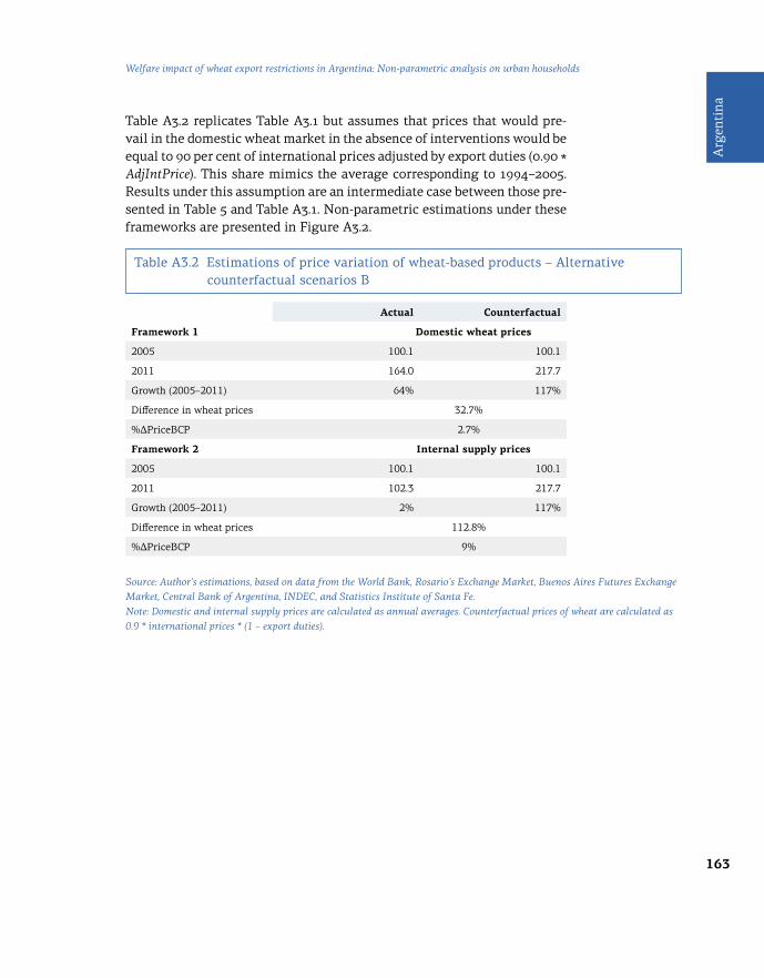
163
Arg
enti
na
Welfare impact of wheat export restrictions in Argentina: Non-parametric analysis on urban households
Source: Author’s estimations, based on data from the World Bank, Rosario’s Exchange Market, Buenos Aires Futures Exchange Market, Central Bank of Argentina, INDEC, and Statistics Institute of Santa Fe. Note: Domestic and internal supply prices are calculated as annual averages. Counterfactual prices of wheat are calculated as 0.9 * international prices * (1 – export duties).
Table A3.2 replicates Table A3.1 but assumes that prices that would pre-vail in the domestic wheat market in the absence of interventions would be equal to 90 per cent of international prices adjusted by export duties (0.90 * AdjIntPrice). This share mimics the average corresponding to 1994–2005. Results under this assumption are an intermediate case between those pre-sented in Table 5 and Table A3.1. Non-parametric estimations under these frameworks are presented in Figure A3.2.
Table A3.2 Estimations of price variation of wheat-based products – Alternative counterfactual scenarios B
Actual Counterfactual
Framework 1 Domestic wheat prices
2005 100.1 100.1
2011 164.0 217.7
Growth (2005–2011) 64% 117%
Difference in wheat prices 32.7%
%∆PriceBCP 2.7%
Framework 2 Internal supply prices
2005 100.1 100.1
2011 102.3 217.7
Growth (2005–2011) 2% 117%
Difference in wheat prices 112.8%
%∆PriceBCP 9%
164
Trade policies, household welfare and poverty alleviation
References
Abbott, P., Hurt, C. and Tyner, W. (2011). “What’s Driving Food Prices in 2011?” Issue Report 2011. Farm Foundation.
Barrett, C. and Dorosh, P. (1996). “Farmers’ Welfare and Changing Food Prices: Nonparametric Evidence from Rice in Madagascar.” American Journal of Agricultural Economics, 78 (3): 656–669.
Beibe, A., Bondolich, C., Fernández Rotelli, M.L., O’Connor, E., Rodríguez, A. and Roggero, M. (2010). “El maíz y el tri-go como motores del desarrollo argentino.” Propuesta de Política Pública. Fundación Agropecuaria para el Desarrollo de Argentina.
Benjamin, D. and Deaton, A. (1993). “Household Welfare and the Pricing of Cocoa and Coffee in Côte d’Ivoire: Lessons from the Living Standard Surveys.” The World Bank Economic Review, 7 (3): 293–318.
Bertello, A. (2013). “Frenan la exportación de harina por el aumento en el precio y las quejas de faltantes.” La Nación, 25 June.
Brambilla, I., Galiani, S. and Porto, G. (2010). “Argentine trade policies in the XX century: 60 years of solitude.” In: Glaeser, E. and Di Tella, R. Eds. Forthcoming in Argentine Exceptionalism. Harvard University, Cambridge MA.
Cameron, A. and Trivedi, P. (2005). Microeconometrics: methods and applications. Cambridge: Cambridge University Press.
Cooke, B. and Robles, M. (2009). “Recent Food Prices Movements: A Time Series Analysis.” IFPRI Discussion Paper No. 00942. International Food Policy Research Institute, Washington DC.
Deaton, A. (1989a). “Household Survey Data and Pricing Policies in Developing Countries.” The World Bank Economic Review, 3 (2): 183–210.
Deaton, A. (1989b). “Rice Prices and Income Distribution in Thailand: A Non-Parametric Analysis.” The Economic Journal, 99 (395): 1–37.
Dequino, D. (2010). “Diagnóstico sobre la transparencia en los subsidios al sector agroalimentario, gas y transporte.” Proyecto Promoviendo Transparencia en la Asignación de Subsidios. Center of Implementation of Public Policies for Equity and Growth, Buenos Aires.
Estrades, C. and Terra, M.I. (2012). “Commodity prices, trade, and poverty in Uruguay.” Food Policy, 37 (1): 58–66.
Gasparini, L., Cicowiez, M. and Sosa Escudero, W. (2013). Pobreza y desigualdad en América Latina. Conceptos, herrami-entas y aplicaciones. First Edition. Centro de Estudios Distributivos, Laborales y Sociales, Universidad Nacional de La Plata (CEDLAS–UNLP). Buenos Aires: Temas.
Gayá, R. and Michalczewsky, K. (2011). “El salto exportador del MERCOSUR en 2003– 2008. Más allá del boom de las materias primas.” Institute for the Integration of Latin America and the Caribbean, Inter-American Development Bank, Washington DC.
Ghezán, G., Mateos, M. and Elverdín, J. (2001). “Impacto de las políticas de ajuste estructural del sector agropecuario y agroindustrial: el caso de Argentina.” Red de Desarrollo Agropecuario. United Nations Economic Commission for Latin America and the Caribbean, Santiago de Chile.
Gilbert, C. (2010). “How to understand high food prices.” Journal of Agricultural Economics, 61 (2): 398–425.

165
Arg
enti
na
Welfare impact of wheat export restrictions in Argentina: Non-parametric analysis on urban households
IERAL (2011). “Cadena de trigo y sus productos derivados.” Documento de Trabajo. Year 17, No. 111. Fundación Mediterránea. Instituto de Estudios sobre la Realidad Argentina y Latinoeamericana (Institute for Studies of Argentine and Latin American Reality), Cordoba.
INDEC (2007). Encuesta Nacional de Gastos de los Hogares. Base de datos gastos de consumo e ingresos. Resumen Metodológico. Instituto Nacional de Estadísticas y Censos (The National Institute of Statistics and Census), Buenos Aires.
Ivanic, M. and Martin, W. (2008). “Implications of higher global food prices for poverty in low-income countries.” Agricultural Economics, 39 (s1): 405–416.
Ivanic, M., Martin, W. and Zaman, H. (2012). “Estimating the Short-Run Poverty Impacts of the 2010-11 Surge in Food Prices.” World Development, 40 (11): 2302–2317.
Koop, F. (2013). “Shortage of wheat affecting price of wheat.” Buenos Aires Herald, 26 June.
Mitchell, D. (2008). “A Note on Rising Food Prices.” Policy Research Working Paper No. 4682. World Bank, Washington DC.
Peri, G. (2009). “Cadenas de producción. Análisis de protección efectiva.” Final Report. Programa de Inserción Agrícola.
Sharma, R. (2011). “Food Export Restrictions: Review of the 2007–2010 Experience and Considerations for Disciplining Restrictive Measures.” FAO Commodity and Trade Policy Research Working Paper No. 32. Food and Agriculture Organization of the United Nations, Rome.
UNCTAD (2012). “Don’t blame the physical markets: financialization is the root cause of oil and commodity price vola-tility.” UNCTAD Policy Brief No. 25. September. Geneva.
Valero-Gil, J. and Valero, M. (2008). “The effects of rising food prices on poverty in Mexico.” Agricultural Economics, 39 (s1): 485–496.
Warr, P. (2008). “World food prices and poverty incidence in a food exporting country: a multihousehold general equi-librium analysis for Thailand.” Agricultural Economics, 39 (s1): 525–537.
Yu, T.-H.E., Tokgoz, S., Wailes, E. and Chavez, E. (2011). “A quantitative analysis of trade policy responses to higher world agricultural commodity prices.” Food Policy, 36 (5): 545–561.

166
Trade policies, household welfare and poverty alleviation
China

167
Chi
na
The consumption effect of the renminbi appreciation in rural China
Abstract
What does the recent appreciation of the renminbi mean for the poor in the People’s Republic of China? This question is rarely asked, and the few responses to date have come in the form of opinions rather than hard ev-idence. The objective of this study is to provide elements of an answer by examining the consumption effect of the renminbi appreciation in rural China. Because households in different regions consume diverse baskets of goods, the main part of this study analyses the impact of the appreci-ation on changes in household consumption (excluding what is self-pro-duced consumption) in response to exchange-rate-induced market price changes, by commodity and by region. The results of the analysis lead to the conclusion that the appreciation of the renminbi has generated signif-icant gains for all households by reducing their consumption expenditure. However, gains have been lower for poorer households, especially those in the inland western provinces of China. The main reason for these lower gains is that households in these provinces spend more on commodities that are less responsive to exchange rate movements. Furthermore, the ex-change rate pass-through and, hence, the impact of the renminbi appreci-ation on market prices, falls with the level of development of the market economy, which is lower in the inland provinces. Consequently, to enhance the positive effect of the renminbi appreciation on these households, the government should step up market development reforms to establish mar-ket-driven pricing mechanisms, in addition to providing households with direct assistance, such as subsidies for poor families.
Dahai Fu and Shantong Li *
* The authors would like to thank Ying Zhang and Yanrui Wu from the University of Western Australia and Yihong Tang from the Central University of Finance and Economics for their comments and suggestions, and the National Social Science Fund of China (Project No. 13CJL037) for co-funding the development of the study.

168
Trade policies, household welfare and poverty alleviation
1 Introduction
The impact of trade liberalization on poverty in developing countries has been widely debated in policy circles and the research community (Hertel and Reimer, 2005). Great efforts have been made to investigate various channels through which trade liberalization might affect the poor (Winters, 2002; Porto, 2006; Goldberg and Pavcnik, 2004, 2007; Nicita, 2009; Topalova, 2010; McCaig, 2011). China – the most populous country in the world – has made poverty reduction one of the priorities of its de-velopment strategy, and has achieved remarkable progress during the past three decades since initiating market reforms in late 1978. However, with China still having the world’s second-largest poor population in absolute terms after India, poverty reduction remains an important challenge for the Chinese government going forward.
China’s Twelfth Five-Year Plan (2011–2015) placed the goal to “reduce poverty and to improve equity in the distribution of income” high on its agenda. General principles, however, are not enough. Appropriate policy formulation calls for detailed quantitative policy analysis. To date, numer-ous studies have examined the evolving pattern and determinants of pov-erty in China (Fang et al., 2002; Yao et al., 2004; Meng et al., 2005; Appleton et al., 2010). Little research has been carried out, however, on the effects of trade liberalization on poverty in China, which is particularly impor-tant for the country at present (Liang, 2007; Huang et al., 2007). In par-ticular, the appreciation of the renminbi (RMB) since July 2005 represents a momentous step forward in Chinese trade liberalization and has had a great impact on the country’s trade flows, labour market, and economic growth. However, its poverty impact has not been addressed in the pub-lished literature.
In July 2005, China ceased to fix its exchange rate against the United States dollar and began to appreciate the RMB. The RMB was no longer solely pegged to the USD, but rather to a basket of currencies, including the USD and the Japanese yen, among others. Since then, the Chinese currency has appreciated over 30 per cent against the USD. Even in terms of the nom-inal effective exchange rate (NEER), it has strengthened by more than 20 per cent. During 2004–2011, the consumer price index (CPI) and real ef-fective exchange rate (REER) also increased, even more rapidly than the NEER, as shown in Figure 1.
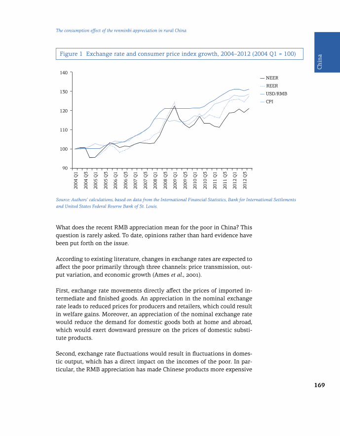
169
Chi
na
The consumption effect of the renminbi appreciation in rural China
Figure 1 Exchange rate and consumer price index growth, 2004–2012 (2004 Q1 = 100)
Source: Authors’ calculations, based on data from the International Financial Statistics, Bank for International Settlements and United States Federal Reserve Bank of St. Louis.
What does the recent RMB appreciation mean for the poor in China? This question is rarely asked. To date, opinions rather than hard evidence have been put forth on the issue.
According to existing literature, changes in exchange rates are expected to affect the poor primarily through three channels: price transmission, out-put variation, and economic growth (Ames et al., 2001).
First, exchange rate movements directly affect the prices of imported in-termediate and finished goods. An appreciation in the nominal exchange rate leads to reduced prices for producers and retailers, which could result in welfare gains. Moreover, an appreciation of the nominal exchange rate would reduce the demand for domestic goods both at home and abroad, which would exert downward pressure on the prices of domestic substi-tute products.
Second, exchange rate fluctuations would result in fluctuations in domes-tic output, which has a direct impact on the incomes of the poor. In par-ticular, the RMB appreciation has made Chinese products more expensive
90
100
110
120
140
130
― NEER
REER
― USD/RMB
― CPI
2004
Q1
2005
Q1
2006
Q1
2007
Q1
2008
Q1
2009
Q1
2010
Q1
2011
Q1
2012
Q1
2004
Q3
2005
Q3
2006
Q3
2007
Q3
2008
Q3
2009
Q3
2010
Q3
2011
Q3
2012
Q3

170
Trade policies, household welfare and poverty alleviation
abroad, and hence negatively affected the exporting sector, which employs a large proportion of unskilled workers who are more likely to come from poor households. Although many regional governments, concerned about labour welfare and social stability, have recently raised the minimum sala-ry by 15–20 per cent, the positive impact of this measure on the poor seems marginal and slow to come to fruition.
Finally, the real exchange rate influences the country’s external compet-itiveness and hence its growth rate, which can affect the poor in the long term through reduced employment opportunities and wages.
Due to data limitations, this study only examines the effect of the RMB appreciation occurring through the price channel. More specifically, it aims to estimate the impact of the RMB appreciation on household wel-fare that arises through exchange-rate-induced changes in consumer pric-es. The research is thus strongly associated with two established strands of literature.
The first strand of literature is related to the estimation of exchange rate pass-through (ERPT) to import prices or domestic prices (Goldberg and Knetter, 1997; Campa and Goldberg, 2006). The starting point in the ex-amination of the price transmission of exchange rate movements is the law of one price (LOP). Most of the evidence indicates that the deviation from the LOP tends to be large and persistent, which points to incomplete ERPT. Empirical studies on ERPT in developing economies have become more frequent in recent years (Choudhri and Hakura, 2006; Devereux and Yetman, 2002; Frankel et al., 2005). A general finding is that the ERPT in de-veloping economies also tends to be incomplete and smaller for consumer prices than for import prices. Few studies covering China have been con-ducted to date. Ca’Zorzi et al. (2007) used the vector autoregressive mod-el for a large number of emerging countries, including China, and found that a 1 per cent change in the exchange rate would lead to a 0.08 per cent change in China’s consumer prices after one year, and 0.77 per cent after two years. Shu et al. (2008) found that a 10 per cent increase in the NEER of the Chinese currency would dampen consumer prices by 1.1 per cent with-in a year. Jin (2012) showed that a 1 per cent appreciation of the NEER re-duced the CPI inflation rate by 0.132 per cent and the producer price index (PPI) inflation rate by 0.495 per cent over the long term from 1996 to 2009.
The second strand of literature is related to studies using household-lev-el data to evaluate the distributional and welfare effects of relative price changes induced by macroeconomic shocks. Examples are Porto (2006), Nicita (2009), Chen and Ravallion (2004), and Ferreira et al. (2004). Porto

171
Chi
na
The consumption effect of the renminbi appreciation in rural China
(2006) and Nicita (2009) studied the impact that a reduction of import tariffs has on household welfare via a fall in domestic prices. Chen and Ravallion (2004) examined the effect of hypothetical relative price chang-es induced by China’s accession to the World Trade Organization (WTO) on household income and consumption in China. Ferreira et al. (2004) used a sectoral disaggregated model to quantify the effects of the depreciation in Brazil on wages and prices, and then link this to a household survey to assess the distributional effects. While many studies have investigat-ed the price effect of tariff liberalization on household welfare, little re-search – except for Kraay (2008) – has been done on the welfare impact of exchange-rate-induced price changes. Kraay (2008) empirically investi-gated the effect of the large depreciation of the Egyptian pound on house-hold welfare between 2000 and 2005. The average welfare loss due to exchange-rate-induced price increases was equivalent to 7.4 per cent of in-itial expenditure.
Following Kraay (2008), this study employs techniques from both strands of literature described above to analyse the case of the significant appre-ciation of the RMB since mid-2005. The potential distributional conse-quences of that appreciation have prompted widespread concern among policymakers. To the best of our knowledge, this study would be the first to combine econometric estimators of ERPT with household survey data to assess the poverty effects of the RMB appreciation. More importantly, in contrast to previous studies, this study estimates relatively disaggre-gated pass-through regressions. Because households in different regions consume diverse sets of commodities, it is necessary to analyse the price changes induced by exchange rate movements by commodity and by re-gion. After obtaining the estimates of the ERPT in the first step, this study further analyses the impact of the ERPT-induced price changes on house-hold welfare by calculating the compensating variations. The empirical re-sults are discussed, and conclusions are provided at the end.
2 Poverty reduction in China
China’s achievement in reducing poverty during the reform era has been remarkable, irrespective of the different alternative approaches to meas-uring poverty, be they in terms of official poverty or international stand-ards, income or consumption, or the absolute number of poor versus the incidence, depth and severity of poverty (World Bank, 2009). Results and estimates on poverty may differ from one source to the other or from one author to the other depending on the approach and the data, but they con-sistently point to the same poverty trends over time.

172
Trade policies, household welfare and poverty alleviation
According to the official rural poverty line,1 more than 250 million peo-ple, or 30.7 per cent of the rural population, lived in poverty in rural China in 1978 (Figure 2). By 2007, the rural poverty rate had decreased dramat-ically to 1.6 per cent. There is no officially established urban poverty line. However, estimates using an urban poverty line comparable to the official rural poverty line found negligible poverty levels in urban areas already in 2002 (Ravallion and Chen, 2007). Both poverty estimates, for rural and urban areas, suggest that China has practically solved its poverty problem.
Figure 2 China’s record of poverty reduction, 1978–2007 (selected years)
Source: Authors’ calculations, based on NBS (2012). Note: This poverty rate is based on the official poverty line of RMB 785 per person per year.
However, as shown by the World Bank (2009), the Chinese government’s task of poverty reduction is not yet complete. The official poverty line re-mains relatively low compared with the international standard of USD 1.25 per day in purchasing power parity (PPP) terms, and also in relation to ris-ing incomes and growing aspirations of the country. The World Bank sta-tistics show that, according to international measures of poverty, there were about 254 million poor people in China in 2005. In addition, vulnera-bility to poverty caused by a variety of income shocks remains widespread.
1 Until 2008, the official poverty line for rural areas in China was RMB 785 per person per year (approximately USD 0.57 per person per day at 2005 PPP prices).
0 0
50 5
10010
15150
20
300
30.7
1.6
35
250 30
20025
■ Millions ― Poverty headcount ratio
1978
1979
1982
1983
1986
1987
1990
1991
1994
1995
1998
1999
2002
2003
2006
1980
1981
1984
1985
1988
1989
1992
1997
2000
2001
2004
2005
2007
Per
cent
Mill
ions
of
peop
le

173
Chi
na
The consumption effect of the renminbi appreciation in rural China
Li et al. 2011 analysed poverty trends between 2002 and 2007 using two waves of household surveys conducted by the China Household Income Project (CHIP) for those years.2 Three alternative poverty estimates are presented in Table 1, two using absolute poverty lines (the 2009 official poverty line3 and the international poverty line of USD 1.25 in PPP terms) and one using a relative poverty line equal to half the median income.4 According to the USD 1.25 poverty line in PPP terms, the incidence of pov-erty in China declined from 18.6 per cent in 2002 to 8 per cent in 2007. This reduction reflects the marked decline in rural poverty, which was due, among other reasons, to the reduction in rural taxes and fees that contrib-uted to a more pro-poor type of growth after 2001. The rapid rise in agricul-tural subsidies (especially for agricultural inputs) and the establishment of rural social assistance programmes (especially Di Bao5 and medical assis-tance) contributed further to the decline in poverty starting in 2005.
Absolute poverty among the registered urban and migrant populations also declined, although it was already rather low in 2002. In contrast, rela-tive poverty measured by the poverty line of 50 per cent of median income remained more or less unchanged at 13 per cent. Stagnant relative poverty rates suggest that households in the lower tail of the income distribution were not catching up to the median, which is consistent with our findings of increased inequality. For all poverty lines, the overwhelming majority of the poor (more than 95 per cent) were living in rural China. For relative poverty, the share of rural poor was lower, but still close to 60 per cent.
2 See the introduction to the sampling procedure of the Chinese National Bureau of Statistics (NBS) 2002 Household Survey, available at: http://www.stats.gov.cn/tjsj/ndsj/yearbook2003 _c.pdf. See also the introduction to the NBS 2007 Household Survey sampling procedure, available at: http://www.stats.gov.cn/tjsj/ndsj/2008/indexch.htm. 3 In 2009, the government raised the official 2008 poverty line to RMB 1,196 (approximately USD 0.87 per person per day at 2005 PPP prices). 4 All the estimates use the official definition of income, which does not include imputed rents from owner-occupied housing. 5 The “Minimum Livelihood Guarantee Scheme”, known as Di Bao in Chinese, was established in 1999. According to the programme’s regulations, individuals whose per capita household income falls below a locally determined minimum living standard can benefit from the programme, irrespective of whether or not they already receive a basic living subsidy, unemployment insurance, or any other insurance.

174
Trade policies, household welfare and poverty alleviation
Table 1 Poverty incidence and composition, 2002 and 2007 (per cent)
Officialpoverty line
PPP USD 1.25per day
50 per centof median income
2002 2007 2002 2007 2002 2007
Poverty incidence
Rural11.22(964)
5.59(1,123)
27.49(1,451)
13.88(1,689)
13.69(1,051)
14.32(1,714)
Urban0.55
(1,338)0.12
(1,503)2.34
(2,013)0.44
(2,260)11.88
(3,379)12.37
(6,412)
Migrants 2.43 0.08 5.80 0.17 18.57 7.00
Total 7.44 3.2 18.57 8.00 13.21 13.3
Poverty composition
Rural 96.72 98.35 95.02 97.70 66.52 60.63
Urban 2.48 1.57 4.21 2.23 30.01 37.73
Migrants 0.8 0.08 0.77 0.07 3.47 1.64
Total 100 100 100 100 100 100
Source: CHIP surveys for 2002 and 2007, and Li et al. (2011).Note: Numbers in parentheses are the poverty lines expressed in RMB. The official rural poverty lines for 2002 and 2007 cor-respond to the 2008 poverty line value (RMB 1,196) adjusted for inflation. Poverty lines for urban areas and migrants are the same. Absolute urban poverty lines are equal to rural poverty lines adjusted by the urban-rural cost of living differential.
Moreover, poverty rates varied significantly across regions. As shown in Table 2, the incidence of absolute poverty in large municipalities, as well as in the eastern part of the country, was extremely low. In the west, the rate of absolute poverty measured using PPP USD 1.25 per day declined from 32 to 15 per cent from 2002 to 2007. Relative poverty was also very low in large municipalities, lower in the east, moderate in central China, and higher in the west, where more than 20 per cent of the population fell below the relative poverty line. Relative poverty nationwide and rel-ative poverty in all regions stayed fairly stable between 2002 and 2007. By all measures, China’s poor are concentrated in the west, where more than half of the absolute poor and over 40 per cent of the relatively poor live. Indeed, the share of the poor in the west increased over this period. The regional structure suggests the need for continuous efforts to allevi-ate poverty, especially in the western and central regions. Furthermore, it is notable that within all regions, poverty is largely rural. For exam-ple, in 2007, in the eastern, central and western regions, the rates of ru-ral poverty measured using USD 1.25 per day were 4, 7 and 15 per cent, respectively. Such a pattern has implications for the design of anti-pov-erty programmes.

175
Chi
na
The consumption effect of the renminbi appreciation in rural China
Table 2 Structure of poverty by region, 2002 and 2007 (per cent)
Source: CHIP surveys for 2002 and 2007, and Li et al. (2011).
Officialpoverty line
PPP USD 1.25 per day
50 per centof median income
2002 2007 2002 2007 2002 2007
Poverty incidence
Big cities 0.07 0.09 0.70 0.35 0.89 1.87
East 3.77 1.59 8.80 3.74 7.73 7.78
Central 6.98 2.74 19.87 7.47 14.21 12.81
West 15.53 6.07 31.64 14.77 20.49 21.99
Total 7.44 3.20 18.57 8.00 13.21 13.30
Poverty composition
Big cities 0.03 0.09 0.12 0.14 0.21 0.44
East 18.33 17.59 17.16 16.51 21.19 20.65
Central 30.42 28.41 34.71 30.94 34.91 31.94
West 51.22 53.91 48.00 52.40 43.69 46.96
Total 100 100 100 100 100 100
Notwithstanding the substantial reduction in poverty in China since 1978, the pace of that reduction has decelerated and new forms of poverty have emerged. Several factors are making it more difficult to reduce poverty, including the deteriorating quality of growth in terms of its potential to generate employment, and increased inequality. Moreover, a high propor-tion of the poverty that persists is geographically dispersed and transient. Poverty has also become less responsive to macroeconomic growth (World Bank, 2009).
3 Methodology and data
The empirical approach used in this study to measure the effects of the RMB appreciation on household welfare in terms of consumption expend-iture is similar to Kraay (2008) and consists of two steps. The first step ties exchange rate changes to disaggregated consumer prices of different goods in different provinces. The second step evaluates the response of consumption expenditure of households to changes in consumer prices. A detailed discussion of each of these steps follows.

176
Trade policies, household welfare and poverty alleviation
3.1 Estimation of the exchange rate pass-through
The key question addressed in the first step is the effect of the RMB ap-preciation on disaggregated consumer prices between 2004 and 2011. Following the standard ERPT models such as Feenstra et al. (1996) and Goldberg and Knetter (1997), we model the consumer price changes as a function of the exchange rate, trade costs, producer prices, prices of im-ported goods, money supply, and domestic demand. Therefore, the estima-tion equation is given by:
CPirt = β0 + β1 ERt + β2 ERt TCr + β3 CPirt-1
+ β4 PPrt + β5 MPt + β6 M2t + β7 TSrt + εit (1)
where CPirt is the monthly price index for good i in region r at time t, which is published based on the current period previous year (CPPY) = 100. Here we work with price indices for food, clothing, medical care, durable goods, education, housing, and transportation and communications, which corre-spond to expenditure categories in the household survey. ERt is the month-ly average of NEERs of China at time t, which is drawn from the Bank for International Settlements.6 We adjust it to be based on CPPY = 100 in or-der to make it consistent with other index data.
Because a primary concern is to measure the effect of exchange rate chang-es on domestic prices at the regional level, following Nicita (2009), we in-clude an interaction term between the trade cost and the exchange rate ( ERt TCr ) to isolate empirically the local effect of exchange rate movements in the pass-through. Rather than measuring the trade cost ( TCr ) by simply using the distance to the border, we use an alternative indicator, namely the marketization index (Fan et al., 2011). The index comprises 19 compo-nents of institutional arrangements and policies in five major areas: (a) size of the government in the regional economy; (b) economic structure, main-ly concerning the growth of the non-state sector and the reform of state enterprises; (c) interregional trade barriers, including price controls; (d) factor market development, including factor mobility; and (e) legal frame-works. Each province has an index between 0 and 10 that measures the rel-ative position in the progress towards a market economy compared with other provinces. It is reasonable to expect that the regions with a high val-ue in the marketization index would be more responsive to exchange rate
6 NEERs are calculated as geometric weighted averages of bilateral exchange rates. The weighting pattern is time-varying, and the most recent weights are based on trade in 2008–2010. For more information, refer to the Bank’s website at: http://www.bis. org/statistics/eer.
177
Chi
na
The consumption effect of the renminbi appreciation in rural China
7 We acknowledge that it would have been better to include the disaggregate PPI for each good, but this was impossible due to the unavailability of data. 8 All data used to estimate the ERPT, except for the NEER, were drawn from the database of the China Economic Information Network, available at: http://db.cei.gov.cn. They were adjusted to be based on CPPY = 100.
movements than those with a low value. The pass-through effects then can be captured by the coefficients of the exchange rate and exchange rate – trade cost variables.
PPrt is the producer price index in region r at time t, which describes the percentage change compared to the same period of the previous year.7 It is included to control for the impact of production costs on consumer prices. As considerable evidence has shown that domestic prices could be affect-ed by the prices of imported goods, we include the price index of imported goods (MPt). Following McCarthy (2000), we also control for the influence of the money supply, which is measured by the percentage change of M2t compared to the same period of the previous year. China’s anchor is to maintain a relative pegging exchange rate, and therefore money supply is always used for price stability (Jin, 2012). Furthermore, we control for the impact of demand on consumer prices by including the variable of total sales in each region (TSrt). It is also a monthly percentage change variable compared with the period of the previous year. Finally, εit is the error term.8
An important issue that arises when working with price equations is that prices tend to have some inertia and persistence in their formation. We need to deal with time dependence and potential autocorrelation prob-lems that may bias our estimates if the data are not properly corrected. In addition, many textbooks suggest that error terms are heteroskedastic and/or serially correlated. According to Baltagi (2008), ignoring the pres-ence of heteroskedastic and/or serially correlated disturbances will gener-ate inefficient standard errors even though the coefficients are consistent. Therefore, we include the lagged dependent variable CPirt-1 in our regres-sion and then perform feasible generalized least squares (FGLS) for the cross-sectional time-series linear model. FGLS estimators are appropriate when one or more of the assumptions of homoskedasticity and non-cor-relation of regression fail. In this case, FGLS estimation is more efficient than pooled ordinary least squares (POLS) estimation, leading to small-er standard errors, narrower confidence intervals, and larger t-statistics (Cameron and Trivedi, 2009). However, the FGLS method cannot deal with the potential endogeneity of the regressors.
The endogeneity problem may result from the two-way relationship be-tween the dependent variable and independent variables, such as CPI and

178
Trade policies, household welfare and poverty alleviation
monetary policies. Furthermore, there would be a time lag effect of ex-change rate changes, production costs, and import prices on domestic pric-es. Therefore, it seems reasonable to use lagged independent variables in our regression. In addition, given the possible serial correlation within panels, we include lagged independent variables for at least two months to explain the current prices. Equation (1) thus could be rewritten as:
CPirt = β0 + β1(L) ERt-n + β2(L) ERt–n TCr + β3 CPirt–2
+ β4 PPrt–2 + β5 MPt–2 + β6 M2t–2 + β7 TSrt–2 + εit (2)
In this empirical model, we lagged all the independent variables two months to alleviate possible bias due to the endogeneity problem. As for the exchange rate variable, we included it in the equation once for each lag ( n >– 2). One advantage of this method is that we could examine the short-term and long-term pass-through while correcting for the possible multicollinearity problem. The ERPT can be captured by the sum of the co-efficients on the exchange rate for each regression.
3.2 Welfare impact of exchange-rate-induced price changes
Having estimated the transmission effect of exchange rate changes to the prices of goods in different regions, it is now possible to evaluate the im-pact of price changes on household welfare. Following Kraay (2008), we employ the compensating variation (CV) to evaluate the welfare effects of price changes.9 The compensating variation measures the change in ex-penditure that would be required for households to achieve their utility level before the external shock (u0) at the price level after the shock (p1). It can be mathematically expressed as:
CV = e ( p1,u0 ) – e (p0,u0 ) (3)
The compensating variation can then be approximated by a second-or-der Taylor expansion of the expenditure function around the initial peri-od prices:
CV ≈ ∆p' ∂e ( p,u0 ) +
1
2 ∆p'
∂2 e ( p,u0 ) ∆p (4)
∂p
∂p∂p'
9 Due to data constraints, we can only analyse the aspect of consumption, although we know that exchange rate movements are also likely to affect household welfare via income and labour market channels. This could be a topic for future research.

179
Chi
na
The consumption effect of the renminbi appreciation in rural China
10 Kraay (2008) considered the role of second-order effects, namely substitution effects, in response to the price changes, but made a restrictive assumption of a diagonal Slutsky matrix, which implies that all compensated cross-price elasticities are zero. The omission of the second-order effects in this study is due to the data limitation, and it might lead to an underestimation of the overall welfare changes due to the appreciation. 11 The estimated results are not presented here for the sake of brevity but are available from the authors upon request. 12 Campa and Goldberg (2006) pointed out that most of the pass-through response occurs over the first and second lagged quarters after the exchange rate change, so the interpretation of six months as short term is empirically validated in our study. In their study, Campa and Goldberg (2006) use lagged four quarters as long-term analysis.
where the matrices of the first and second derivatives of the expenditure function are evaluated at the price level before the shock (p0). Estimating the substitution effects, however, requires data on goods prices at the household level. In the case of CHIP survey data, we do not have informa-tion on unit values for individual consumption items. We therefore stick to the first-order effect, namely, the direct effect of price changes resulting from exchange rate movements.10 In particular, we can further write the direct effect of price changes as a share of initial expenditure, in a weight-ed average of the growth rate of the prices of each good, with weights (wi) equal to initial expenditure shares:
∆p' x0 ≈ ∑ wi ∆pi ––– ∑
pi0 xi0 ∆pi (5)――–– —–– ――––– —––
e0 pi e0 pi
From the perspective of consumption, a household is worse off if prices go up, and better off if prices go down.
4 Results and discussion
4.1 Estimations of the exchange rate pass-through to consumer prices
The ERPT to consumer prices for seven categories of expenditure items is estimated separately.11 Based on these estimates, we calculate the short-term ERPT as the sum of the coefficients on the lagged exchange rate var-iables and their interaction terms, with the trade costs measured by the marketization index.12 The estimates of the short-term impact of the ex-change rate on consumer prices for each province and good are present-ed in Table 3. The coefficients in the table reflect the percentage change of consumer prices induced by a 1 per cent change in the NEER of the renminbi.
i i( ) ( )( )
180
Trade policies, household welfare and poverty alleviation
More specifically, we find that the pass-through of exchange rate move-ments to consumer prices is incomplete and varies substantially across products and regions. The estimates show that the RMB appreciation has lowered consumer prices of goods, except for medical care and durable goods. One potential explanation is that the elasticity of substitution be-tween domestic medicines and imported ones is low. Residents rely on domestic medicines and medical services, and rarely use imported alter-natives. Therefore, consumers are less likely to gain from the appreciation of the domestic currency in the short term. For durable goods – such as tel-evisions, refrigerators, air-conditioners, fans, washing machines, and mi-crowaves – the exchange rate movement has had little influence on their price and there are no regional variations. One possible explanation is that Chinese manufacturers dominate the household appliance sector. China is now the world’s largest manufacturer, with over 50 per cent of its pro-duction sold in overseas markets. Price competition in the home market is fierce and, therefore, these goods are rarely affected by the appreciation.
In comparison, the RMB appreciation has significantly reduced prices of food and housing expenditure. On average, a 1 per cent change in the ex-change rate is translated into 0.345 per cent decrease in the consumer price of food. The degree of ERPT for the consumer price of housing expendi-ture, including purchase, construction costs, and maintenance and repairs, is even higher, reaching 0.479 per cent under the same circumstances. The most likely reason is that the RMB appreciation has led to a decrease in the price of fuel (Yang et al., 2012), which constitutes a large part of variations in the price of food and housing expenditure. This suggests that consumer prices of food and housing expenditure may be relatively more responsive to exchange rate changes. With respect to clothing, the ERPT is low, about 0.03 per cent for each province. In addition, we find no regional variance in ERPT for clothing. This is mainly because production and consumption of clothing in China are highly domestic-oriented. The exchange rate move-ment has little impact on the sector's inputs and final products. Finally, the estimates of pass-through for education, and transportation and communi-cations are also low, about 0.09 per cent.
Furthermore, we find that the variations of ERPT for different items across the provinces are low – less than 1 per cent. However, in general, we can see that retail prices seem to be more responsive to exchange rate changes in provinces with a high marketization index. This can be expected because the provinces with a more developed market economy are also located in coastal regions, and are more closely linked to foreign markets.

181
Chi
na
The consumption effect of the renminbi appreciation in rural China
Table 3 Pass-through estimates for each province (per cent)
Source: Authors’ estimations.
Province Food Clothing Medical care
Durable goods
Education Housing Transportation & communications
Anhui –0.345 –0.031 0.0948 0.001 –0.093 –0.478 –0.089
Beijing –0.351 –0.031 0.0947 0.001 –0.100 –0.490 –0.090
Chongqing –0.347 –0.031 0.0948 0.001 –0.095 –0.482 –0.089
Gansu –0.338 –0.031 0.0949 0.001 –0.086 –0.466 –0.087
Guangdong –0.356 –0.031 0.0946 0.001 –0.105 –0.497 –0.091
Guangxi –0.343 –0.031 0.0948 0.001 –0.090 –0.474 –0.088
Guizhou –0.339 –0.031 0.0949 0.001 –0.086 –0.467 –0.087
Hebei –0.344 –0.031 0.0948 0.001 –0.092 –0.477 –0.089
Henan –0.344 –0.031 0.0948 0.001 –0.092 –0.476 –0.089
Hubei –0.345 –0.031 0.0948 0.001 –0.093 –0.479 –0.089
Hunan –0.345 –0.031 0.0948 0.001 –0.093 –0.478 –0.089
Jiangsu –0.353 –0.031 0.0947 0.001 –0.101 –0.492 –0.090
Jiangxi –0.344 –0.031 0.0948 0.001 –0.092 –0.476 –0.089
Jilin –0.343 –0.031 0.0948 0.001 –0.091 –0.475 –0.088
Liaoning –0.349 –0.031 0.0947 0.001 –0.097 –0.485 –0.090
Shaanxi –0.339 –0.031 0.0949 0.001 –0.087 –0.468 –0.088
Shandong –0.350 –0.031 0.0947 0.001 –0.098 –0.487 –0.090
Shanxi –0.341 –0.031 0.0949 0.001 –0.088 –0.471 –0.088
Sichuan –0.346 –0.031 0.0948 0.001 –0.094 –0.480 –0.089
Xinjiang –0.340 –0.031 0.0949 0.001 –0.088 –0.470 –0.088
Yunnan –0.340 –0.031 0.0949 0.001 –0.088 –0.470 –0.088
Zhejiang –0.353 –0.031 0.0947 0.001 –0.101 –0.492 –0.090
Mean –0.345 –0.031 0.0948 0.001 –0.093 –0.479 –0.089
Standard deviation
0.005 0.000 0.000 0.000 0.005 0.009 0.001

182
Trade policies, household welfare and poverty alleviation
4.2 Welfare impact of exchange-rate-induced price changes
We first use 2002 CHIP survey data for rural areas to calculate the initial consumption structure for each household.13 In particular, when we calcu-late the share of food consumption, we focus only on the food consumption paid in cash, as this is expected to be more responsive to price changes. In rural China, a substantial part of food consumption, particularly cere-als and vegetables, comes from self-production rather than expenditure in cash. However, the meat and fish consumed are usually purchased on the market. Table 4 presents average consumption shares of different items across the provinces in 2002. It shows that food has the largest share in the consumption basket, accounting for one quarter on average. Moreover, we find that the share of food consumption varies significantly across provinc-es, ranging from 19.4 to 33 per cent. One reason for this variation is differ-ences in the levels of regional economic development (Zhou et al., 2003). For instance, Guangdong is the most developed province in China, while Anhui is at a medium level of development and Gansu is the least devel-oped. In the developed provinces, rural residents have less farm land, but more opportunities to work in factories and thus buy more food on the market. On the other hand, residents from less developed regions have to produce food for themselves. Moreover, each province is also quite differ-ent in terms of culture, traditions, and other aspects of social life. These factors contribute to the different consumption patterns in different prov-inces. The share of housing expenditure is about 11.2 per cent, and all other consumption shares are lower than 10 per cent. The share of consumption of durable goods is the smallest, about 1 per cent.
Table 5 presents summary statistics of household income and expendi-ture per capita for different groups of households for 2002–2003 (when the survey was conducted), and a share of total consumption expenditure that households spend on food, clothing, medical care, durable goods, education, housing, and transportation and communications. Coastal households are richer than those inland in terms of average income and expenditure per capita. Inland households earn and spend less than the national average. However, these differences do not seem very large. When we classify house-holds according to the international poverty line of USD 1.25 per day, we find that, on average, poor households spend 1.3 per cent less on food items than those living above the poverty line, but spend more on non-food items. This finding may seem surprising, since poor households usually tend to spend a higher share of expenditure on food than richer households. One should however bear in mind that we have excluded consumption of self-produced goods, which represents a substantial share of total consumption for poor households. This may reduce the differences in consumption patterns.

183
Chi
na
The consumption effect of the renminbi appreciation in rural China
Table 4 Consumption shares across provinces (per cent)
Source: Authors’estimations.
Province Food Clothing Medical care
Durable goods
Education Housing Transportation & communications
Anhui 25.4 3.9 2.4 1.0 7.3 12.8 5.7
Beijing 33.2 4.9 1.3 3.2 6.7 12.8 7.1
Chongqing 23.5 4.7 0.1 0.8 5.6 9.2 5.1
Gansu 19.4 6.1 4.2 1.3 10.7 10.7 4.7
Guangdong 30.6 3.3 2.4 0.9 9.5 11.6 8.4
Guangxi 20.2 3.5 2.2 0.6 8.1 12.6 4.9
Guizhou 19.5 6.1 1.8 1.3 9.5 9.4 3.8
Hebei 30.1 10.5 2.2 0.9 5.2 13.5 7.4
Henan 24.2 8.7 3.3 1.3 9.0 11.9 6.2
Hubei 21.5 5.7 1.0 0.8 2.9 10.5 6.0
Hunan 23.4 9.8 2.7 0.5 8.6 8.7 4.3
Jiangsu 25.0 6.4 2.6 2.6 2.4 11.5 6.7
Jiangxi 22.4 5.3 3.7 0.7 6.3 12.7 6.6
Jilin 28.3 7.0 4.9 0.7 7.7 15.1 7.9
Liaoning 27.9 7.4 3.0 0.6 3.5 10.9 6.9
Shaanxi 21.5 6.5 6.8 0.8 19.5 11.8 4.3
Shandong 28.7 6.7 5.4 2.1 12.3 10.0 6.0
Shanxi 29.0 8.8 1.8 1.3 8.6 10.3 6.6
Sichuan 21.0 5.2 2.9 0.8 6.1 9.6 4.7
Xinjiang 24.6 10.7 1.6 0.6 0.9 9.7 4.3
Yunnan 21.0 3.2 1.8 0.9 3.1 8.7 3.3
Zhejiang 32.6 4.8 4.7 1.7 7.2 11.9 9.2
Average 25.2 6.4 3.0 1.1 7.4 11.2 6.0
13 Rural and urban areas are classified according to Hukou, a residence registration system formally set up in 1958 that divides the population into rural and urban households. This study focuses on rural areas, as we find that most people living below the poverty line are concentrated in rural China. Moreover, only the 2002 CHIP survey reports information on the consumption structure of households in rural areas, and it is necessary to make the strong assumption that the budget share based on this survey remained essentially unchanged during the examined period.
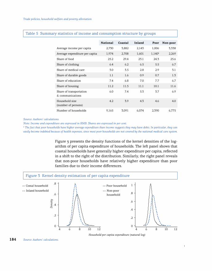
184
Trade policies, household welfare and poverty alleviation
Table 5 Summary statistics of income and consumption structure by groups
National Coastal Inland Poor Non-poor
Average income per capita 2,730 3,882 2,143 1,006 3,338
Average expenditure per capita 1,974 2,708 1,601 1,140§ 2,269
Share of food 25.2 29.4 23.1 24.3 25.6
Share of clothing 6.4 6.2 6.5 5.5 6.7
Share of medical care 3.0 3.5 2.8 2.9 3.1
Share of durable goods 1.1 1.6 0.9 0.7 1.3
Share of education 7.4 6.8 7.0 7.7 6.7
Share of housing 11.2 11.5 11.1 10.1 11.6
Share of transportation & communications
6.0 7.4 5.3 3.7 6.9
Household size (number of persons)
4.2 3.9 4.3 4.6 4.0
Number of households 9,165 3,091 6,074 2,390 6,775
Source: Authors’ calculations.Note: Income and expenditure are expressed in RMB. Shares are expressed in per cent.§ The fact that poor households have higher average expenditure than income suggests they may have debts. In particular, they can easily become indebted because of health expenses, since most poor households are not covered by the national medical care system.
Source: Authors’ calculations.
Figure 3 presents the density functions of the kernel densities of the log-arithm of per capita expenditure of households. The left panel shows that coastal households have generally higher expenditure per capita, reflected in a shift to the right of the distribution. Similarly, the right panel reveals that non-poor households have relatively higher expenditure than poor families due to their income differences.
Figure 3 Kernel density estimation of per capita expenditure
.8 1
0 06 64 48 810 1012 12
.2.2
.4
.4
.6
.6
.8
― Costal household
Inland household
― Poor household
Non-poor household
Household per capita expenditure (natural log)
Den
sity
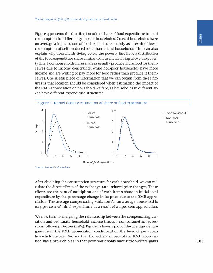
185
Chi
na
The consumption effect of the renminbi appreciation in rural China
Figure 4 Kernel density estimation of share of food expenditure
Source: Authors’ calculations.
Figure 4 presents the distribution of the share of food expenditure in total consumption for different groups of households. Coastal households have on average a higher share of food expenditure, mainly as a result of lower consumption of self-produced food than inland households. This can also explain why households living below the poverty line have a distribution of the food expenditure share similar to households living above the pover-ty line. Poor households in rural areas usually produce more food for them-selves due to income constraints, while non-poor households have more income and are willing to pay more for food rather than produce it them-selves. One useful piece of information that we can obtain from these fig-ures is that location should be considered when estimating the impact of the RMB appreciation on household welfare, as households in different ar-eas have different expenditure structures.
After obtaining the consumption structure for each household, we can cal-culate the direct effects of the exchange-rate-induced price changes. These effects are the sum of multiplications of each item's share in initial total expenditure by the percentage change in its price due to the RMB appre-ciation. The average compensating variation for an average household is 0.14 per cent of initial expenditure as a result of a 1 per cent appreciation.
We now turn to analysing the relationship between the compensating var-iation and per capita household income through non-parametric regres-sions following Deaton (1989). Figure 5 shows a plot of the average welfare gains from the RMB appreciation conditional on the level of per capita household income. We see that the welfare impact of the RMB apprecia-tion has a pro-rich bias in that poor households have little welfare gains
4 4
0 0.2 .20 0.4 .4.6 .6.8 .81 1
1 1
2 2
3 3
― Poor household
Non-poor household
― Coastal household
Inland household
Den
sity
Share of food expenditure

186
Trade policies, household welfare and poverty alleviation
from the appreciation. This result is mainly driven by differences in con-sumption patterns between these two types of households. Poor house-holds spend less on food and housing, which become cheaper as a result of the appreciation, but usually spend more on medical care, the price of which has not decreased following the appreciation.
Figure 5 Non-parametric regression results – Overall welfare
Source: Authors’ calculations.Note: The dependent variable is the change in household welfare measured by the compensating variation.
Figure 6 shows similar regressions for coastal and inland households. We find that there is no big difference in welfare gains between poor and rich households in the coastal provinces. One possible reason is that poor households in these provinces have consumption patterns with regard to food that are similar to those of rich households. Poor households in coast-al regions do not consume much self-produced food. They usually work in rural enterprises or as migrant workers in cities and buy a large propor-tion of food on the market. The other reason is that medical care and the educational system are well developed in coastal regions and poor house-holds thus get better financial support in this regard compared to those inland. However, there is a significantly positive relationship between wel-fare gains and income per capita for households living in the inland prov-inces. The welfare gain of the richest households is about twice that of the poorest households. Also interesting to note in Figure 6 is that the effects of appreciation are greater in coastal areas than in inland provinces, con-ditional on per capita household income. This is because coastal provinces
.05
.1
.15
.2
.25■ 95% confidence intervals
― Ipoly smooth
4 6 8 102Household per capita income (natural log)
Wel
fare
cha
nge

187
Chi
na
The consumption effect of the renminbi appreciation in rural China
Figure 6 Non-parametric regression results – Coastal versus inland households
Source: Authors’ calculations.Note: The dependent variable is the change in household welfare measured by the compensating variation.
are more integrated into the world market via trade and foreign direct in-vestment and are therefore more responsive to the appreciation.
To show the heterogeneous welfare effects of the appreciation-induced price changes across regions, we calculated the average compensating var-iations along the quintile of income distribution for each province (see Annex). We found a positive relationship between the average compensat-ing variation and the marketization level at the provincial level, which is illustrated in Figure 7. This suggests that people living in provinces with a more developed market economy could gain more from the RMB appre-ciation. This may be explained by the fact that provinces with a well-func-tioning economy are more responsive to exchange rate changes. Another explanation could be that these provinces are located in coastal regions and thus closer to foreign markets. In addition, the estimated compensat-ing variations vary significantly across regions, ranging from a low of 11.1 per cent in Yunnan Province to a high of 18.2 per cent in Beijing. Within most provinces, the welfare gains increase with the average income of the household. However, there are also some exceptions. For example, the poorest household in Beijing gains 9.1 per cent more than the richest household. In Zhejiang, the relationship becomes U-shaped. These region-al heterogeneities could be explained by the differences in consumption structures and ERPT across provinces.
.08
.1
.12
.14
.16
.18
4 6 8 102Household per capita income (natural log)
― Coastal household
Inland household
Wel
fare
cha
nge

188
Trade policies, household welfare and poverty alleviation
Figure 7 Compensating variation and marketization index
Source: Authors’ calculations.
5 Conclusions
This study estimated the consumption impact of appreciation of the ren-minbi, with particular attention to its effect on poor households in the People’s Republic of China. The analysis was conducted in two steps. First, we investigated the impact of exchange rate changes on domestic prices, namely the ERPT, using disaggregated monthly consumer price indices between 2004 and 2011. Second, we used household surveys to investigate the consumption effects of price changes induced by exchange rate move-ments. Without information on labour income, we were only able to ex-amine the price channel through which exchange rate changes influence household welfare. Using the information on consumption expenditure for each household from the CHIP survey data for 2002, we first calculated the consumption structure and then estimated the direct effects induced by the price changes.
The main results show that the price transmission from exchange rate changes to retail prices is incomplete and heterogeneous across consump-tion items and regions. Generally speaking, the RMB appreciation is found to drive down domestic prices of goods, except for medical care and du-rable goods. Moreover, the exchange rate changes are transmitted to con-sumer prices of food and housing to a higher degree than in the case of
.1
.12
.14
.16
.18 Compensating variation
― Fitted values
6 8 104
Marketization index

189
Chi
na
The consumption effect of the renminbi appreciation in rural China
other consumption items. A 1 per cent appreciation reduces the prices of food and housing by 0.345 and 0.479 per cent, respectively. From the per-spective of regional heterogeneity, it is found that consumer prices in provinces with a higher marketization level are highly responsive to ex-change rate movements. Such diversity in ERPT is then expected to have a different welfare impact on people living in different regions.
According to estimates of compensating variations, we find that all house-holds could experience gains from the RMB appreciation, although the magnitude of the effect looks small in the short term, equivalent to only 3 per cent of initial expenditure. In addition, the estimated compensating variation associated with the direct effect of exchange-rate-induced price changes is on average lower for poorer households. However, there is enor-mous heterogeneity across households and regions. The magnitude of the benefits is highly associated with consumption structures and locations of households.
We should nevertheless keep in mind that there are at least two caveats regarding the results of this study. The first is that we have only examined the impact of the exchange rate changes on household welfare that oc-curs through the consumption channel. The appreciation is also expected to have heterogeneous impacts on the income of households employed in different sectors. It is widely accepted that the RMB appreciation has been a challenge for the exporting sector, which employs a large number of un-skilled labour from poor households in rural areas. It is plausible that as a result of the appreciation, households employed in the exporting sector would see decreases in earnings while those working in import-competing industries would see increases in earnings. The negative income effects due to the RMB appreciation could be large enough to offset the limited consumption benefits, and lead to an increase in poverty. Unfortunately, we could not empirically investigate these effects and their distributional consequences in any detail due to the lack of detailed employment infor-mation in the household survey.
The second caveat is that we conducted the analysis at a relatively aggre-gate level, since there is no information regarding a more disaggregated set of expenditure items in the official statistics and the household sur-vey. Therefore, we could only estimate the direct effect of price changes induced by the appreciation, disregarding the substitution effects. As a re-sult, we are likely to be underestimating the effects on household welfare. In addition, we should keep in mind that omission of self-produced food in our analysis might underestimate the welfare changes for poor house-holds, since they usually produce food for themselves. Thus, we have to be

190
Trade policies, household welfare and poverty alleviation
cautious about making conclusions with regard to the total effect of the RMB appreciation on household welfare.
In spite of these caveats, we can still draw some policy implications from our results. The RMB appreciation could bring benefits for households by reducing their consumption expenditure. However, poor households in ru-ral areas of inland provinces would gain less. Anti-poverty policies should therefore take into account regional heterogeneity – such as the consump-tion pattern of residents and the development level of the market economy – because according to our research these factors play an important role in the welfare effects of exchange rate changes.
Prices of food, which represents a large share of expenditure for the poor-est households, have fallen more than prices of other items as a result of the RMB appreciation. This seems beneficial for the poor. However, poor households, especially those living in the inland provinces, usual-ly produce a large proportion of food such as grain and vegetables for themselves. Therefore, they cannot reap the benefits of the food price de-crease induced by the RMB appreciation. In contrast, the reduced food prices may lower the income of poor rural households in inland provinces, meaning that these may therefore not only gain less from lower consump-tion expenditure, but also suffer from the income effect of the apprecia-tion. Therefore, the Chinese government should provide subsidies for poor families and pay attention to the fundamental factors that drive inflation. Furthermore, given the limited welfare gains from price transmission, the government should pay attention to labour market effects that are like-ly to affect the poor. Such effects are related to the negative impact of the RMB appreciation on the Chinese manufacturing export sector, which em-ploys a large number of unskilled workers who are more likely to come from poor households.

191
Chi
na
The consumption effect of the renminbi appreciation in rural China
Annex
Table A1 Estimated compensation variation by region and quintile of income distribution
Source: Authors’ calculations.Note: Compensation variation results from 1 per cent appreciation of the RMB.
Quintile of income distribution
Mean Lowest Second Third Fourth Highest
Anhui 0.150 0.142 0.143 0.149 0.162 0.165
Beijing 0.182 0.262 0.221 0.193 0.175 0.171
Chongqing 0.129 0.112 0.122 0.133 0.134 0.140
Gansu 0.120 0.112 0.123 0.132 0.131 0.123
Guangdong 0.174 0.158 0.170 0.160 0.170 0.182
Guangxi 0.130 0.135 0.127 0.120 0.141 0.164
Guizhou 0.114 0.103 0.117 0.128 0.143 0.169
Hebei 0.170 0.195 0.162 0.177 0.158 0.162
Henan 0.145 0.149 0.137 0.147 0.145 0.152
Hubei 0.124 0.122 0.123 0.123 0.120 0.137
Hunan 0.129 0.116 0.131 0.131 0.134 0.137
Jiangsu 0.144 0.155 0.143 0.133 0.138 0.150
Jiangxi 0.139 0.143 0.132 0.136 0.137 0.154
Jilin 0.170 0.187 0.174 0.167 0.159 0.166
Liaoning 0.152 0.152 0.147 0.149 0.152 0.157
Shaanxi 0.140 0.137 0.138 0.133 0.160 0.163
Shandong 0.159 0.149 0.153 0.149 0.159 0.175
Shanxi 0.153 0.146 0.148 0.152 0.156 0.176
Sichuan 0.121 0.124 0.114 0.117 0.120 0.150
Xinjiang 0.128 0.129 0.129 0.127 0.131 0.117
Yunnan 0.111 0.110 0.112 0.107 0.118 0.096
Zhejiang 0.179 0.180 0.159 0.162 0.180 0.186
Average 0.144 0.146 0.142 0.142 0.147 0.154

192
Trade policies, household welfare and poverty alleviation
References
Ames, B., Brown, W., Devarajan, S. and Izquierdo, A. (2001). Macroeconomic Policy and Poverty Reduction. International Monetary Fund and World Bank, Washington DC.
Appleton, S., Song, L. and Xia, Q. (2010). “Growing Out of Poverty: Trends and Patterns of Urban Poverty in China 1988–2002.” World Development, 38 (5): 665–678.
Baltagi, B.H. (2008). Econometric Analysis of Panel Data. Fourth Edition. Chichester: Wiley.
Cameron, A.C. and Trivedi, P.K. (2009). Microeconometrics Using Stata. College Station: Stata Press.
Campa, J.M. and Goldberg, L.S. (2006). “Pass-through of Exchange Rates to Consumption Prices: What Has Changed and Why?” NBER Working Paper No. 12547. National Bureau of Economic Research, Cambridge MA.
Ca’Zorzi, M., Hahn, E. and Sánchez, M. (2007). “Exchange Rate Pass-through in Emerging Markets.” ECB Working Paper No. 739. European Central Bank, Frankfurt.
Chen, S. and Ravallion, M. (2004). “Welfare Impacts of China’s Accession to the World Trade Organization.” The World Bank Economic Review, 18 (1): 29–57.
Choudhri, E.U. and Hakura, D.S. (2006). “Exchange Rate Pass-through to Domestic Prices: Does the Inflationary Environment Matter?” Journal of International Money and Finance, 25 (4): 614–639.
Deaton, A. (1989). “Rice Prices and Income Distribution in Thailand: A Non-Parametric Analysis.” The Economic Journal, 99 (395): 1–37.
Devereux, M.B. and Yetman, J. (2002). “Price Setting and Exchange Rate Pass-through: Theory and Evidence.” Hong Kong Institute for Monetary Research Working Paper No. 22/2002.
Fan, G., Wang, X. and Zhu, H. (2011). Marketization Index Report in China: Marketization Process across Regions in 2010. Beijing: Economic Science Press.
Fang, C., Zhang, X. and Fan, S. (2002). “Emergence of Urban Poverty and Inequality in China: Evidence from Household Survey.” China Economic Review, 13 (4): 430–443.
Feenstra, R.C., Gagnon, J.E. and Knetter, M.M. (1996). “Market Share and Exchange Rate Pass-through in World Automobile Trade.” Journal of International Economics, 40 (1): 187–207.
Ferreira, F., Leite, P., Silva, L.P.D. and Picchetti, P. (2004). “Can the Distributional Impact of Macroeconomic Shocks be Predicted? A Comparison of the Performance of Macro-Micro Models with Historical Data for Brazil.” Policy Research Working Paper No. 3303. World Bank, Washington DC.
Frankel, J.A., Parsley, D.C. and Wei, S.J. (2005). “Slow Pass-through around the World: A New Import for Developing Countries?” NBER Working Paper No. 11199. National Bureau of Economic Research, Cambridge MA.
Goldberg, P.K. and Knetter, M.M. (1997). “Goods Prices and Exchange Rates: What Have We Learned?” Journal of Economic Literature, 35 (3): 1243–1272.
193
Chi
na
The consumption effect of the renminbi appreciation in rural China
Goldberg, P.K. and Pavcnik, N. (2004). “Trade, Inequality, and Poverty: What Do We Know? Evidence from Recent Trade Liberalization Episodes in Developing Countries.” NBER Working Paper No. 10593. National Bureau of Economic Research, Cambridge MA.
Goldberg, P.K. and Pavcnik, N. (2007).“Distributional Effects of Globalization in Developing Countries.” Journal of Economic Literature, 45 (1): 39–82.
Hertel, T.W. and Reimer, J.J. (2005). “Predicting the Poverty Impacts of Trade Reform.” Journal of International Trade and Economic Development, 14 (4): 377–405.
Huang, J., Jun, Y. and Xu, Z. (2007). “Agricultural Trade Liberalization and Poverty in China.” China Economic Review, 18 (3): 244–265.
Jin, X. (2012). “An Empirical Study of Exchange Rate Pass-Through in China.” Panoeconomicus, 59 (2): 135–156.
Kraay, A. (2008). “The Welfare Effects of a Large Depreciation: The Case of Egypt 2000¬–2005.” In: Kheir-El-Din, H. Ed. The Egyptian Economy: Current Challenges and Future Prospects. Cairo: The American University in Cairo Press.
Li, S., Luo, C. and Sicular, T. (2011). “Overview: Income Inequality and Poverty in China, 2002–2007.” CIBC Working Paper No. 201110. Centre for Human Capital and Productivity, University of Western Ontario.
Liang, Z. (2007). “Trade Liberalization, Economic Restructuring and Urban Poverty: The Case of China.” Asian Economic Journal, 21 (3): 239–259.
McCaig, B. (2011). “Exporting Out of Poverty: Provincial Poverty in Vietnam and U.S. Market Access.” Journal of International Economics, 85 (1): 102–113.
McCarthy, J. (2000). “Pass-through of Exchange Rates and Import Prices to Domestic Inflation in Some Industrialized Economies.” BIS Working Paper No. 79. Bank for International Settlements, Basel.
Meng, X., Gregory, B. and Wang, Y. (2005). “Poverty, Inequality, and Growth in Urban China, 1986–2000.” Journal of Comparative Economics, 33 (4): 710–729.
NBS (2012). Poverty Monitoring Report of Rural China 2011. Household Survey Department, National Bureau of Statistics, Beijing.
Nicita, A. (2009). “The Price Effect of Tariff Liberalization: Measuring the Impact on Household Welfare.” Journal of Development Economics, 89 (1): 19–27.
Porto, G. (2006). “Using Survey Data to Assess the Distributional Effects of Trade Policy.” Journal of International Economics, 70 (1): 140–160.
Ravallion, M. and Chen, S. (2007). “China’s (Uneven) Progress against Poverty.” Journal of Development Economics, 82 (1): 1–42.
Shu, C., Su, X. and Chow, N. (2008). “Exchange Rate Pass-through in Mainland China.” China Economic Issues, 1 (8). Hong Kong Monetary Authority.
Topalova, P. (2010). “Factor Immobility and Regional Impacts of Trade Liberalization: Evidence on Poverty from India.” American Economic Journal: Applied Economics, 2 (4): 1–41.

194
Trade policies, household welfare and poverty alleviation
Winters, L.A. (2002). “Trade Liberalisation and Poverty: What Are the Links?” The World Economy, 25 (9): 1339–1367.
World Bank (2009). From Poor Areas to Poor People: China’s Evolving Poverty Reduction Agenda. World Bank, Washington DC.
Yang, J., Zhang, W. and Tokgoz, S. (2012). “The Macroeconomic Impacts of Chinese Currency Appreciation on China and the Rest of World.” IFPRI Discussion Paper No. 01178. International Food Policy Research Institute, Washington DC.
Yao, S., Zhang, Z. and Hanmer, L. (2004). “Growing Inequality and Poverty in China.” China Economic Review, 15 (2): 145–163.
Zhou, Z., Wu, Y. and Tian, W. (2003). “Food Consumption in Rural China: Preliminary Results from Household Survey Data.” Proceedings of the 15th Annual Conference of Association for Chinese Economics Studies Australia (ACESA), 2–3 October.

195
Chi
na
The consumption effect of the renminbi appreciation in rural China

196
Trade policies, household welfare and poverty alleviation
Costa Rica

197
Cos
ta R
icaWelfare effects of a change in the trade
policy regime for rice in Costa Rica
Abstract
The rice market in Costa Rica has several distinctive features. First, rice is an essential staple in the diet of Costa Ricans, particularly for the poorest segments of the population. Second, while rice is produced in the country, local production does not reach the level necessary to satisfy domestic de-mand. Third, rice imports have been subject to policy measures targeting both local production and imports, including a performance requirement for the importation of paddy rice from the United States. Fourth, a price-fix-ing mechanism designed as part of the policy package applied to the rice sector has increased paddy rice prices paid to local producers to double that of international prices. As a result, Costa Rican consumers have been paying a high price for a key commodity in their daily consumption basket. Despite the associated costs, the policies cited above have not been suc-cessful in either increasing productivity or improving conditions for small farmers. Costa Rica is also in breach of its World Trade Organization com-mitments as a result of the distortionary support received by producers through the price-fixing mechanism. For these reasons, Costa Rica’s poli-cies related to the rice sector are being redesigned. For example, the free trade agreement between Central America, the Dominican Republic and the United States will provide unlimited duty-free access for imports from the United States in 2025. This study shows that poor households in Costa Rica may be the segment of the population that will benefit the most from a reduction in the price of rice. In this sense, the free trade agreement may be an opportunity to effectively reduce rice prices in the domestic market and thus improve the welfare of consumers.
* The author would like to thank Henry Benavides and Karen Chan from the Ministry of Foreign Trade of Costa Rica for their support in the preparation of this study.
Carlos Eduardo Umaña-Alvarado *

198
Trade policies, household welfare and poverty alleviation
1 Introduction
In recent years there has been an ongoing discussion in Costa Rica about the trade policy regime for rice. Rice is an essential product in the daily diet of Costa Ricans. According to the 2004 National Income and Expenditure Survey (ENIG),1 rice is one of the most important products for the lowest (one through four) income quintiles. For example, rice represented 4.97 per cent of expenditure in the first quintile and, taken together, quintiles one and two accounted for 48 per cent of rice consumption in the country (Arroyo et al., 2013). Based on these figures, a reduction in the price of rice would mainly benefit the poorest groups of the population.
Rice policies in Costa Rica are based on a combination of tariffs, a perfor-mance requirement for the importation of paddy rice,2 and a price-fixing mechanism. The combined effect of these measures creates economic dis-tortions in the sector. According to economic theory, market price sup-port raises domestic producer and consumer prices. This results in an increase in production and a reduction in consumption, an equivalent of a welfare transfer from consumers to producers. Therefore, a market price support system distorts both production and consumption decisions (Umaña, 2011).
This mechanism is regressive in terms of incomes, as per capita spend-ing on rice is relatively more important in low-income households. In ad-dition, the level of distortionary subsidies resulting from the minimum producer price in Costa Rica exceeds by more than five times the lev-el stipulated in the country’s World Trade Organization (WTO) commit-ments. This situation has led to consultations at the WTO with partners concerned about the Costa Rican measures.
Several studies have specifically analysed Costa Rica’s rice policies. According to Umaña (2011), import protection and price controls for rice in Costa Rica have not increased yields, but created instead significant rents for rice millers by transferring income from consumers to producers,
1 ENIG stands for Encuesta Nacional de Ingresos y Gastos. At the time of this analysis, the 2004 survey was the most recent source of information on household consumption in Costa Rica. 2 The performance requirement allocated to the millers is the right to import paddy rice in an amount proportional to the purchase of the local harvest. 3 According to Umaña (2011), tariffs, water subsidies and price controls have not benefited small farmers, as millers have largely captured the rents associated with protectionism. Furthermore, it is hard for small farms to achieve economies of scale, a factor relevant for the efficiency of rice production.

199
Cos
ta R
ica
Welfare effects of a change in the trade policy regime for rice in Costa Rica
and by maintaining local prices above international prices for years. Nor have the rice policies improved the livelihood of small and independ-ent farmers,3 or promoted the expansion of consumption opportunities for the poorest households. Because most mills are vertically integrat-ed, they have favoured imports instead of dealing with the risky process of rice farming in the country. Gains from trade have thus benefited mill-ers, as these firms have captured the rents from lower international pric-es (Umaña, 2011).
Arroyo et al. (2013) describe the main features of the rice market in Costa Rica and conclude that the pricing scheme is not contributing to impor-tant policy objectives such as increasing productivity and improving the access of consumers to affordable rice. Many producers receive lower prices compared to the fixed price due to the difference in rice qualities (inferior qualities are punished with lower prices), consumers pay prices above international prices, productivity remains stagnant or downward, and the pricing scheme may be working towards increasing costs of some inputs and services used in rice production. In addition, Petrecolla (2006) estimates that income transfers from consumers to the rice industry (pro-ducers and processors) reached a cumulative USD 396.4 million from 1996 to 2005. Of these transfers, 80 per cent were captured by processors and only 20 per cent by farmers. During the same period, millers, wholesalers, and retailers preserved their margins.
Costa Rica has entered into the free trade agreement between Central America, the Dominican Republic, and the United States (CAFTA-DR) that will provide unlimited duty-free access to imports from the United States when the phasing-out schedule ends in 2025. The agreement may be an opportunity to effectively reduce rice prices in the domestic market and thus improve consumers’ welfare.
In this context, this study aims to quantify the welfare effects of the phas-ing-out process and the quotas stipulated in the CAFTA-DR. By assuming a perfect transmission of changes in tariffs to domestic prices, the study presents a forecast of the welfare effects for three different scenarios: for 2015, 2020, and 2025.
The study uses Costa Rica’s 2004 National Income and Expenditure Survey, along with a forecast of the evolution of prices based on the CAFTA-DR phasing-out scheme, to undertake a non-parametric analysis. The results show that a reduction in rice prices will benefit consumers, particular-ly the poorest households for whom rice represents a larger share of to-tal expenditure. However, in order to prevent importers from capturing

200
Trade policies, household welfare and poverty alleviation
new rents from the reduction of import tariffs, rice prices may need to be monitored on an ongoing basis. This task could be entrusted to the enti-ties that are in charge of competition policies and consumers’ interests, such as the Commission for the Promotion of Competition (COPROCOM).4
The next section describes developments in the rice sector in Costa Rica and the international trade regime for rice. The methodology applied in the study is then presented, followed by a discussion of the welfare impli-cations of a reduction in the price of rice for households. The study then puts forward several policy recommendations and concludes with a sum-mary of the main findings of the research.
2 The rice sector in Costa Rica
2.1 Production
Rice cultivation accounts for 3.9 per cent of total value added of agricultur-al, livestock, and fisheries production in Costa Rica (SEPSA, 2012). During the 2011–2012 harvest, 1,355 producers were engaged in rice production in the country. Micro and small producers represent approximately 80 per cent of the total number of farmers, but they cultivate only around 20 per cent of the total rice-planted land (Table 1). Medium-sized producers, with farms between 50 and 200 hectares (ha), and large farmers, with farms larger than 200 ha, supply 80 per cent of national production. After 1950, the rice sector underwent a structural change towards the organization of production in large and medium-sized agro-enterprises; today, small farms only account for a small share of total production (Arroyo et al., 2013).
4 COPROCOM stands for Comisión para Promover la Competencia. Its fundamental purpose is to protect and promote free competition, as well as investigate and punish monopolistic practices and other restrictions to the efficient functioning of the market. For more details, see the organization’s website at: http://www.coprocom.go.cr. 5 CONARROZ stands for Corporación Arrocera Nacional, which is an institution composed of producers, millers and the government that supports Costa Rica’s rice sector by promot- ing good relationships between farmers and millers and the overall development of the sector. CONARROZ manages a parafiscal fund financed by a 1.5 per cent contribution levied on the price of delivered rice, which is paid both by producers and millers, and by a 1.5 per cent levy on the price of imported rice that is paid by importers. The purpose of the fund is to enable CONARROZ to fulfill the duties entrusted to it by Law No. 8285.

201
Cos
ta R
ica
Welfare effects of a change in the trade policy regime for rice in Costa Rica
6 CONARROZ, Informes Estadísticos, various issues.
Type of producer
Size of farm Number of
producers
Hectares planted
Share of area planted
(per cent)
Average size of area
(hectares)
Micro Less than 10 ha 542 3,118 4.0 5.8
Small Between 10 and 50 ha 528 12,633 16.4 23.9
Medium Between 50 and 200 ha 222 21,611 28.0 97.3
Large More than 200 ha 63 39,877 51.6 633.0
Total 1’355 7,240 100.0 56.9
Table 1 Structure of rice production, 2011–2012
Source: CONARROZ.
Between the harvests of 2000–2001 and 2005–2006, Costa Rica experienced a downward trend in paddy rice yields, which fell annually by 2.2 per cent, reaching 3.35 metric tons per ha during the 2005–2006 harvest (Figure 1). The decline in yields that occurred during the 2004–2006 period coincid-ed with the emergence in the country of the acarus Steneotarsonemus spinki, which caused major losses in the sector, and an increase in production costs, according to the National Rice Corporation (CONARROZ).5 During the subsequent two harvests, yields recovered up to 3.78 metric tons per ha. However, they declined again for the 2010–2012 harvest to settle at 3.39 metric tons per ha.6
Met
ric
tons
per
hec
tare
3.9
3.8
3.7
3.6
3.5
3.4
3.3
2000
/01
2001
/02
2002
/03
2003
/04
2004
/05
2005
/06
2006
/07
2007
/08
2008
/09
2009
/10
2010
/11
2011
/12
Figure 1 Paddy rice yield, 2000–2001 to 2011–2012 (metric tons per hectare)
Source: CONARROZ.
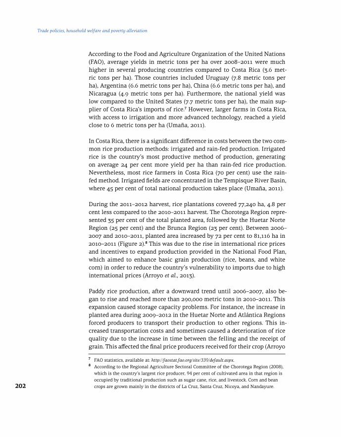
202
Trade policies, household welfare and poverty alleviation
According to the Food and Agriculture Organization of the United Nations (FAO), average yields in metric tons per ha over 2008–2011 were much higher in several producing countries compared to Costa Rica (3.6 met-ric tons per ha). Those countries included Uruguay (7.8 metric tons per ha), Argentina (6.6 metric tons per ha), China (6.6 metric tons per ha), and Nicaragua (4.9 metric tons per ha). Furthermore, the national yield was low compared to the United States (7.7 metric tons per ha), the main sup-plier of Costa Rica’s imports of rice.7 However, larger farms in Costa Rica, with access to irrigation and more advanced technology, reached a yield close to 6 metric tons per ha (Umaña, 2011).
In Costa Rica, there is a significant difference in costs between the two com-mon rice production methods: irrigated and rain-fed production. Irrigated rice is the country’s most productive method of production, generating on average 24 per cent more yield per ha than rain-fed rice production. Nevertheless, most rice farmers in Costa Rica (70 per cent) use the rain-fed method. Irrigated fields are concentrated in the Tempisque River Basin, where 45 per cent of total national production takes place (Umaña, 2011).
During the 2011–2012 harvest, rice plantations covered 77,240 ha, 4.8 per cent less compared to the 2010–2011 harvest. The Chorotega Region repre-sented 35 per cent of the total planted area, followed by the Huetar Norte Region (25 per cent) and the Brunca Region (23 per cent). Between 2006–2007 and 2010–2011, planted area increased by 72 per cent to 81,116 ha in 2010–2011 (Figure 2).8 This was due to the rise in international rice prices and incentives to expand production provided in the National Food Plan, which aimed to enhance basic grain production (rice, beans, and white corn) in order to reduce the country’s vulnerability to imports due to high international prices (Arroyo et al., 2013).
Paddy rice production, after a downward trend until 2006–2007, also be-gan to rise and reached more than 290,000 metric tons in 2010–2011. This expansion caused storage capacity problems. For instance, the increase in planted area during 2009–2012 in the Huetar Norte and Atlántica Regions forced producers to transport their production to other regions. This in-creased transportation costs and sometimes caused a deterioration of rice quality due to the increase in time between the felling and the receipt of grain. This affected the final price producers received for their crop (Arroyo
7 FAO statistics, available at: http://faostat.fao.org/site/339/default.aspx. 8 According to the Regional Agriculture Sectoral Committee of the Chorotega Region (2008), which is the country’s largest rice producer, 94 per cent of cultivated area in that region is occupied by traditional production such as sugar cane, rice, and livestock. Corn and bean crops are grown mainly in the districts of La Cruz, Santa Cruz, Nicoya, and Nandayure.
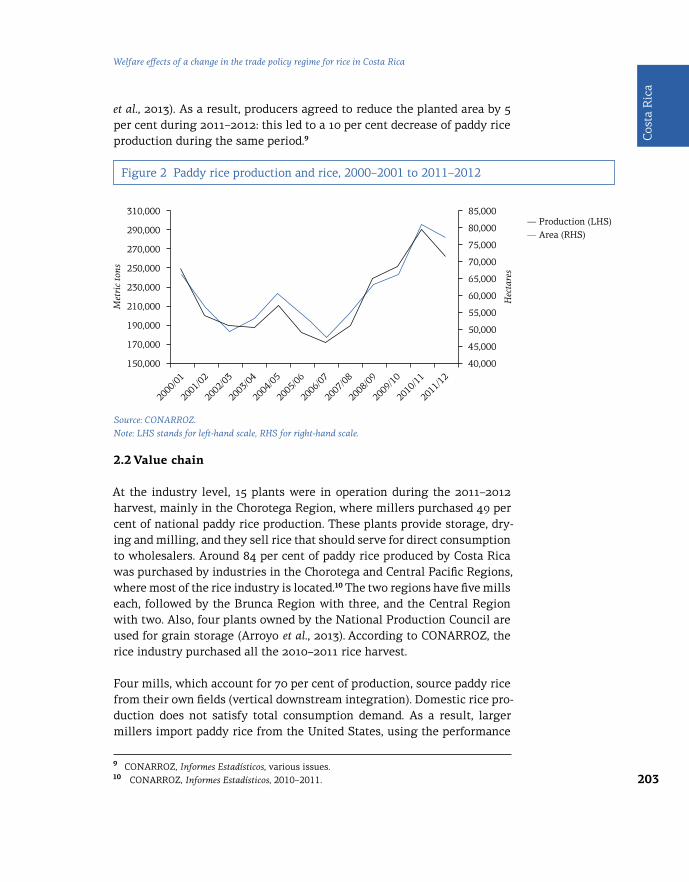
203
Cos
ta R
ica
Welfare effects of a change in the trade policy regime for rice in Costa Rica
Source: CONARROZ.Note: LHS stands for left-hand scale, RHS for right-hand scale.
et al., 2013). As a result, producers agreed to reduce the planted area by 5 per cent during 2011–2012: this led to a 10 per cent decrease of paddy rice production during the same period.9
9 CONARROZ, Informes Estadísticos, various issues. 10 CONARROZ, Informes Estadísticos, 2010–2011.
Figure 2 Paddy rice production and rice, 2000–2001 to 2011–2012
310,000
290,000
270,000
250,000
230,000
210,000
190,000
170,000
150,000
85,000
80,000
75,000
70,000
65,000
60,000
55,000
50,000
45,000
40,000
2000
/01
2001
/02
2002
/03
2003
/04
2004
/05
2005
/06
2006
/07
2007
/08
2008
/09
2009
/10
2010
/11
2011
/12
Met
ric
tons
Hec
tare
s
― Production (LHS) ― Area (RHS)
2.2 Value chain
At the industry level, 15 plants were in operation during the 2011–2012 harvest, mainly in the Chorotega Region, where millers purchased 49 per cent of national paddy rice production. These plants provide storage, dry-ing and milling, and they sell rice that should serve for direct consumption to wholesalers. Around 84 per cent of paddy rice produced by Costa Rica was purchased by industries in the Chorotega and Central Pacific Regions, where most of the rice industry is located.10 The two regions have five mills each, followed by the Brunca Region with three, and the Central Region with two. Also, four plants owned by the National Production Council are used for grain storage (Arroyo et al., 2013). According to CONARROZ, the rice industry purchased all the 2010–2011 rice harvest.
Four mills, which account for 70 per cent of production, source paddy rice from their own fields (vertical downstream integration). Domestic rice pro-duction does not satisfy total consumption demand. As a result, larger millers import paddy rice from the United States, using the performance

204
Trade policies, household welfare and poverty alleviation
requirement applied for the CAFTA-DR quota to keep the mills operating (Umaña, 2011; Arroyo et al., 2013).11
During 2000–2012, milled rice stocks at the end of each month aver-aged 56,600 metric tons. These stocks increased between 2009 and 2012, reaching a maximum of 111,182 metric tons in November 2011, enough to cover 5.8 months with an average consumption of 19,000 metric tons. The increase in stocks of equivalent milled rice was relat-ed to the increased production promoted in the National Food Plan, which set a target of covering 80 per cent of consumption through do-mestic production. To achieve this goal, the sown area increased, but the ability to receive, dry, and store rice did not follow. Consequently, during the peak harvest months (September and October), there were not enough facilities to dry and store the grain (Arroyo et al., 2013).
Between 2000–2001 and 2003–2004, milled rice sales grew at a 6.6 per cent annual average rate. The most significant expansion occurred during 2007–2008, when sales rose by 10.3 per cent compared to the 2006–2007 harvest (Figure 3). However, the subsequent four harvest periods reported lower sales, from 246,130 metric tons in 2007–2008 down to 225,169 metric tons in 2011–2012 (an 8.5 per cent decrease).12 According to millers, this reduc-tion may have been caused by the entry of 6,000 metric tons of milled rice imported by third parties (supermarket chains and wholesalers) under the tariff rate quota (TRQ) scheme of the CAFTA-DR (Arroyo et al., 2013).
11 Section 2.4.2 explains the performance requirement applied by Costa Rica for the paddy rice import quota from the United States under the CAFTA-DR. 12 CONARROZ, Informes Estadísticos, various issues.
Figure 3 Milled rice sales by domestic industries, 2000–2001 to 2011–2012 (metric tons)
Source: CONARROZ.
2000
/01
2001
/02
2002
/03
2003
/04
2004
/05
2005
/06
2006
/07
2007
/08
2008
/09
2009
/10
2010
/11
2011
/12
250,000
240,000
230,000
220,000
210,000
200,000
190,000
180,000
Met
ric
tons
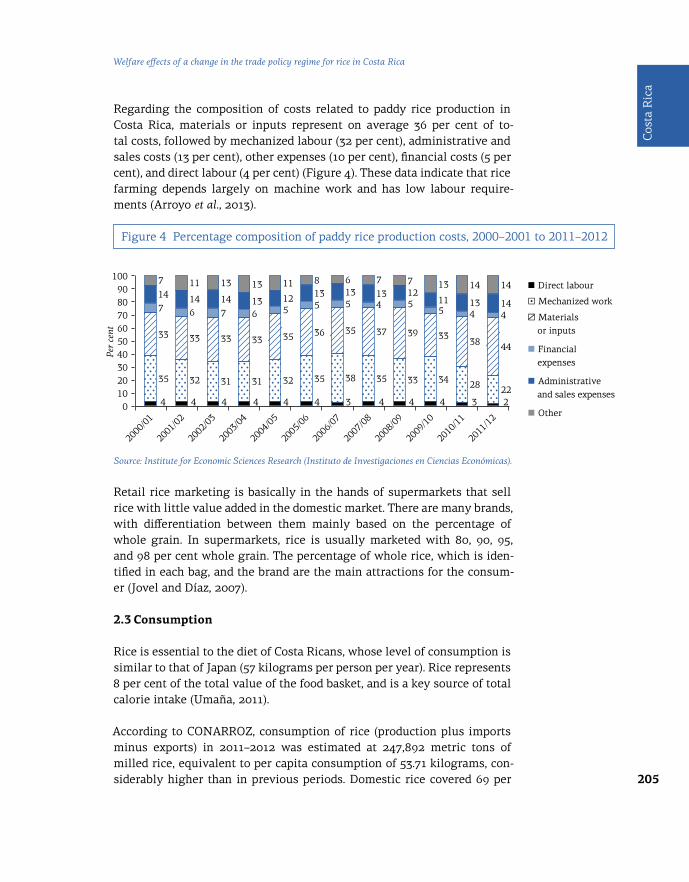
205
Cos
ta R
ica
Welfare effects of a change in the trade policy regime for rice in Costa Rica
Figure 4 Percentage composition of paddy rice production costs, 2000–2001 to 2011–2012
Source: Institute for Economic Sciences Research (Instituto de Investigaciones en Ciencias Económicas).
Regarding the composition of costs related to paddy rice production in Costa Rica, materials or inputs represent on average 36 per cent of to-tal costs, followed by mechanized labour (32 per cent), administrative and sales costs (13 per cent), other expenses (10 per cent), financial costs (5 per cent), and direct labour (4 per cent) (Figure 4). These data indicate that rice farming depends largely on machine work and has low labour require-ments (Arroyo et al., 2013).
■ Direct labour
□ Mechanized work
□ Materials or inputs
■ Financial expenses
■ Administrative and sales expenses
■ Other
1009080706050403020100
2000
/01
2001
/02
2002
/03
2003
/04
2004
/05
2005
/06
2006
/07
2007
/08
2008
/09
2009
/10
2010
/11
2011
/12
33
35
4 4 4 4 4 4 4 4 4 3 23
32
7
714 14 14
13 13
136 5 5 5
6 7 713 13 13
13 1412
11 134 55 4 4
14
148
12
11
6
11
33 33
7
31 31
33 35
32
36
35 38
35 37
35
39
33
33
34 28
38 44
22
Retail rice marketing is basically in the hands of supermarkets that sell rice with little value added in the domestic market. There are many brands, with differentiation between them mainly based on the percentage of whole grain. In supermarkets, rice is usually marketed with 80, 90, 95, and 98 per cent whole grain. The percentage of whole rice, which is iden-tified in each bag, and the brand are the main attractions for the consum-er (Jovel and Díaz, 2007).
2.3 Consumption
Rice is essential to the diet of Costa Ricans, whose level of consumption is similar to that of Japan (57 kilograms per person per year). Rice represents 8 per cent of the total value of the food basket, and is a key source of total calorie intake (Umaña, 2011).
According to CONARROZ, consumption of rice (production plus imports minus exports) in 2011–2012 was estimated at 247,892 metric tons of milled rice, equivalent to per capita consumption of 53.71 kilograms, con-siderably higher than in previous periods. Domestic rice covered 69 per
Per
cent

206
Trade policies, household welfare and poverty alleviation
cent of national consumption, with imported rice accounting for the re-maining 31 per cent. The shortfall of rice to meet domestic consumption was covered by imports from the CAFTA-DR quota and other rice imports.
Rice consumption remained between 230,000 and 238,000 metric tons be-tween 2006–2007 and 2010–2011 (Figure 5), with a spike in consumption towards the end of the period.
Figure 5 National consumption of milled equivalent rice, 2001–2002 to 2011–2012 (metric tons)
Source: CONARROZ.
13 The Costa Rican population increased by almost 20 per cent from 2001 to 2012. 14 Throughout this study, expenditure is used as a proxy for income.
Although total consumption has increased, per capita consumption has re-mained steady since the mid-1990s. This suggests that the growth in na-tional consumption is mainly due to the increase of the population (Arroyo et al., 2013).13
Based on the 2004 ENIG, Table 2 shows the share of household expendi-ture on each type of rice compared to total rice expenditure, by per capita expenditure decile.14 Throughout all income deciles, whole rice with qual-ity classification (e.g. 92 per cent whole grain) is the type that accounts for the highest expenditure share, followed by rice without a quality classifi-cation (e.g. rice produced by households, which includes self-production) and pre-cooked rice.
250,000
240,000
245,000
230,000
235,000
220,000
225,000
210,000
205,000
215,000
200,000
2001
/02
2002
/03
2003
/04
2004
/05
2005
/06
2006
/07
2007
/08
2008
/09
2009
/10
2010
/11
2011
/12
Met
ric
tons
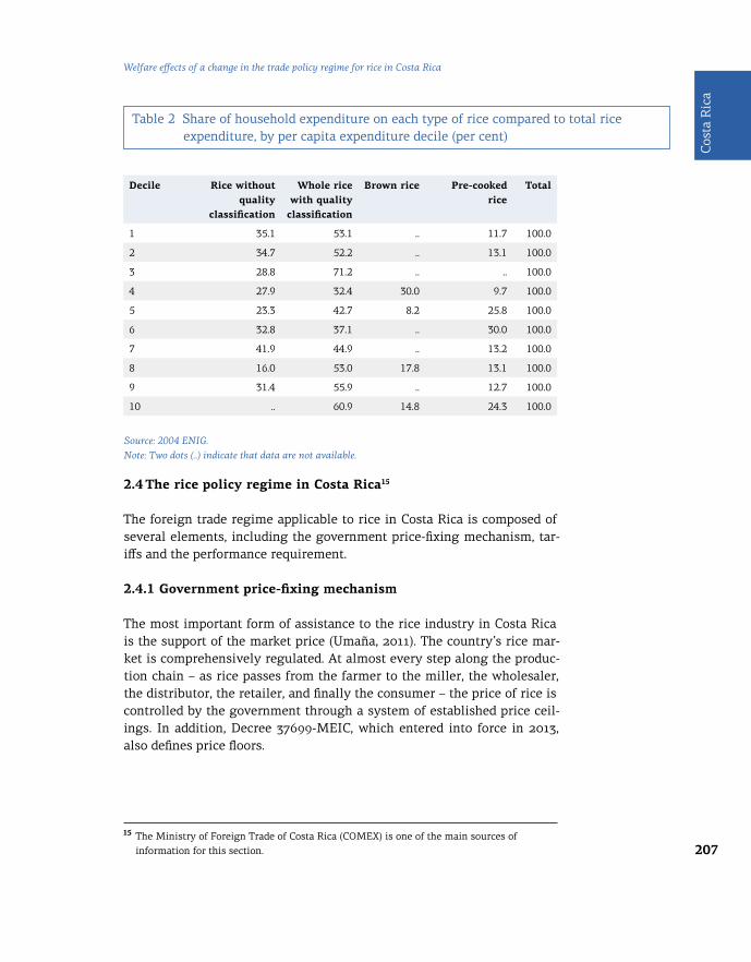
207
Cos
ta R
ica
Welfare effects of a change in the trade policy regime for rice in Costa Rica
2.4 The rice policy regime in Costa Rica15
The foreign trade regime applicable to rice in Costa Rica is composed of several elements, including the government price-fixing mechanism, tar-iffs and the performance requirement.
2.4.1 Government price-fixing mechanism
The most important form of assistance to the rice industry in Costa Rica is the support of the market price (Umaña, 2011). The country’s rice mar-ket is comprehensively regulated. At almost every step along the produc-tion chain – as rice passes from the farmer to the miller, the wholesaler, the distributor, the retailer, and finally the consumer – the price of rice is controlled by the government through a system of established price ceil-ings. In addition, Decree 37699-MEIC, which entered into force in 2013, also defines price floors.
Table 2 Share of household expenditure on each type of rice compared to total rice expenditure, by per capita expenditure decile (per cent)
Source: 2004 ENIG. Note: Two dots (..) indicate that data are not available.
Decile Rice without quality
classification
Whole rice with quality classification
Brown rice Pre-cooked rice
Total
1 35.1 53.1 .. 11.7 100.0
2 34.7 52.2 .. 13.1 100.0
3 28.8 71.2 .. .. 100.0
4 27.9 32.4 30.0 9.7 100.0
5 23.3 42.7 8.2 25.8 100.0
6 32.8 37.1 .. 30.0 100.0
7 41.9 44.9 .. 13.2 100.0
8 16.0 53.0 17.8 13.1 100.0
9 31.4 55.9 .. 12.7 100.0
10 .. 60.9 14.8 24.3 100.0
15 The Ministry of Foreign Trade of Costa Rica (COMEX) is one of the main sources of information for this section.

208
Trade policies, household welfare and poverty alleviation
Rice should be purchased at the official price set by the Ministry of Economy, Industry and Commerce (MEIC). CONARROZ recommends the price for producers, and based on that recommendation, the MEIC defines prices for the other steps of the value chain. The price-fixing mechanism includes the official definition of a purchase price for the rice industry to buy from producers. This model considers an internal cost structure with a profit margin. The calculation is based on an irrigated farm of 250 ha, and considers all costs in the production of paddy rice assigned to the consum-able units of each good and the respective costs, including a profit margin of 20 per cent on costs, excluding financial expenses (COMEX et al., 2010).
The officially established price for producers increased significantly from USD 305 per metric ton in 2006 to USD 633 in 2010, which represents a 107 per cent increase in four years (see Annex 2, Table A2.2). Furthermore, when comparing the officially established price during 1995–2010 with the international price of GL55/70 rice, which is the type of rice imported by Costa Rica, the country’s official price remained significantly higher than the international market price.
As shown in Figure 6, the transmission of the international price to Costa Rican households is direct when the trend is on the rise, but not when in-ternational prices fall. Between 2008 and 2010, the gap between the two prices widened considerably (COMEX et al., 2010). Given that the definition of the producer price considers an internal cost structure, and due to the increase in the cost of inputs, the government raised the producer price.
Imported milled rice is currently sold at the floor prices defined in Decree 37699-MEIC, which are calculated on the basis of the price for domestic producers. This allows the imported milled rice, which has highly compet-itive prices, to fetch a greater profit margin compared to domestic milled rice. Similarly, importers (millers) of paddy rice, which has a much lower price than that paid to domestic producers, use this low-cost raw material in their production processes and capture profits defined by the above de-cree for each stage in the rice value chain.
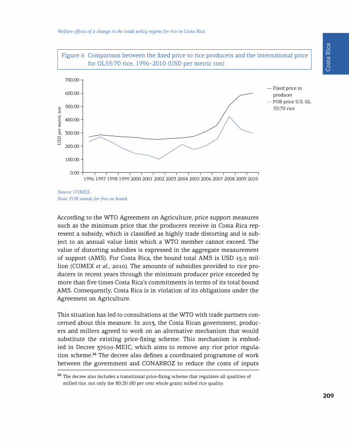
209
Cos
ta R
ica
Welfare effects of a change in the trade policy regime for rice in Costa Rica
Figure 6 Comparison between the fixed price to rice producers and the international price for GL55/70 rice, 1996–2010 (USD per metric ton)
Source: COMEX.Note: FOB stands for free on board.
According to the WTO Agreement on Agriculture, price support measures such as the minimum price that the producers receive in Costa Rica rep-resent a subsidy, which is classified as highly trade distorting and is sub-ject to an annual value limit which a WTO member cannot exceed. The value of distorting subsidies is expressed in the aggregate measurement of support (AMS). For Costa Rica, the bound total AMS is USD 15.9 mil-lion (COMEX et al., 2010). The amounts of subsidies provided to rice pro-ducers in recent years through the minimum producer price exceeded by more than five times Costa Rica’s commitments in terms of its total bound AMS. Consequently, Costa Rica is in violation of its obligations under the Agreement on Agriculture.
This situation has led to consultations at the WTO with trade partners con-cerned about this measure. In 2013, the Costa Rican government, produc-ers and millers agreed to work on an alternative mechanism that would substitute the existing price-fixing scheme. This mechanism is embod-ied in Decree 37699-MEIC, which aims to remove any rice price regula-tion scheme.16 The decree also defines a coordinated programme of work between the government and CONARROZ to reduce the costs of inputs
0.00
100.00
1996 1997 1998 1999 2000 2001 2002 2003 2004 2005 2006 2007 2008 2009 2010
200.00
300.00
400.00
500.00
600.00
700.00
USD
per
met
ric
ton
― Fixed price to producer
― FOB price U.S. GL 55/70 rice
16 The decree also includes a transitional price-fixing scheme that regulates all qualities of milled rice, not only the 80/20 (80 per cent whole grain) milled rice quality.

210
Trade policies, household welfare and poverty alleviation
(agrochemicals and seeds), and prioritizes the implementation of a com-plementary agenda aimed at increasing productivity in the rice sector.17
In June 2013, the country’s decision to reduce its rice subsidies was wel-comed by WTO members as an achievement both for Costa Rica in bring-ing its support back within its WTO commitments, and also for the role of the WTO Agriculture Committee in solving possible contentious issues.18
2.4.2 Current import regime: Tariffs and the performance requirement under the CAFTA-DR
Costa Rica has traditionally been a net importer of rice. In recent years, imports of milled rice have mainly come from the United States and oth-er countries in the Americas.19 In 2012, 84 per cent of Costa Rica’s imports came from the United States, 8.6 per cent from Central America, 4.9 per cent from Argentina, and 2.1 per cent from Uruguay.20 During 1995–2009, the average size of imports and national production relative to total do-mestic supply was 37.9 per cent and 65.2 per cent, respectively (see Annex 2, Table A2.1). However, in recent years, domestic production has been con-tributing more to national consumption of rice due to the stimulus from the price-fixing mechanism.
The bound tariff for Costa Rica in the WTO on paddy and milled rice is 35 per cent; the most-favoured-nation (MFN) tariff for pre-cooked rice is 15 per cent.21 In addition, Costa Rica applies a phytosanitary fee of USD 20 per metric ton (equivalent to around 5 per cent of the international price based on figures of 13 March 2013).
The import of rice from any country in Central America is duty-free un-der the Central American Common Market (CACM). Within the CAFTA-DR,
17 The complementary agenda includes the adoption of: (a) good agricultural practices manuals and a Technology Development Plan for the rice sector; (b) agribusiness training, maintenance, and business management; and (c) a process to strengthen credit mechanisms. 18 “Members welcome Costa Rica’s decision to bring its rice subsidies within agreed limits”, WTO press release, 13 June 2013. Available at: http://www.wto.org/english/news_e/news13_e/ag com_13jun13_e.htm. 19 There is a phytosanitary ban imposed on rice originating from South-East Asia due to Trogoderma granarium. Although the risks associated with this pest have been estimated as being very low, the ban is still enforced. 20 Figures from COMEX, based on data from the Central Bank of Costa Rica. 21 The MFN tariff applied by Costa Rica to rice includes an additional duty of 1 per cent pursuant to Law No. 6946; this duty is applicable to all imports, with a few exceptions As a result, the MFN tariff for paddy and milled rice is 36 per cent, equivalent to the sum of the bound tariff (35 per cent) and the 1 per cent additional duty from Law No. 6946.

211
Cos
ta R
ica
Welfare effects of a change in the trade policy regime for rice in Costa Rica
Costa Rica granted a duty-free import quota of 51,000 metric tons of paddy rice to the United States, which is increasing by 1,000 metric tons per year until 2024. This quota is allocated to the millers. In order to be granted a part of the import quota, millers must first purchase rice from domestic producers. The performance requirement here relates to the right to im-port rice only in an amount proportional to the purchase of the local har-vest (Umaña, 2011).
There are two types of rice millers in Costa Rica: non-integrated independ-ent producers with greater business risk, and integrated mills with lower business risk (Arroyo et al., 2013). The latter often source rice from their own fields. Vertical integration of mills causes the rents of large produc-ers to be added as they move through each step of their chain (production, manufacturing, and wholesale) as the mechanism guarantees a minimum price at the different levels (COMEX et al., 2010). In addition, prices re-ceived by rice millers are higher compared to their competitors in major exporting countries. Costa Rican millers have benefited from prices that are consistently above world market levels due to the protectionist poli-cies that have been implemented (Umaña, 2011).
The local mills also are the largest rice producers, so higher domestic pric-es of rice increase their income. Also, an increase in local prices of rice makes paddy rice imports from the United States relatively cheaper, and, as a result, a larger margin is left for millers when they process and final-ly sell this imported rice in the domestic market. But not only local mills benefit from a high price to producers. Small producers also gain, although large producers enjoy economies of scale and higher productivity levels that allow them to obtain greater benefits from an increase in rice prices.
As part of the commitments defined by the CAFTA-DR, rice was placed in a non-linear 20- year phasing-out category.22 The objective is for the out-of-quota rice imports from the United States to be duty-free in 2025.23 The base rate will remain in 2006–2015, but starting from 2016 (until 2020), tariffs will be reduced by 8 per cent annually, and after 1 January 2021 (until 2024), by 12 per cent per year. The CAFTA-DR should ultimately liberalize rice trade between Costa Rica and the United States, which af-ter the 20-year phase-out period should be completely duty-free. At that
22 The CAFTA-DR entered into force in Costa Rica in 2009; however, the tariff phasing-out schedule started in 2006, when El Salvador began to implement the CAFTA-DR. 23 Prior to the CAFTA-DR, the tariff rate for imports of paddy and milled rice from the United States was 36 per cent. There was no quota providing preferential treatment to these imports.
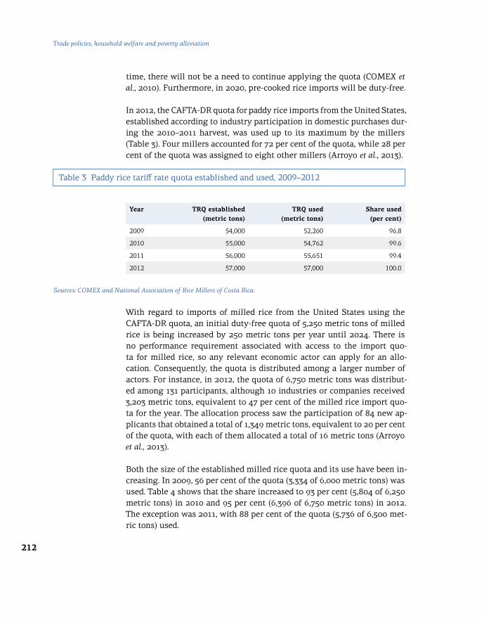
212
Trade policies, household welfare and poverty alleviation
time, there will not be a need to continue applying the quota (COMEX et al., 2010). Furthermore, in 2020, pre-cooked rice imports will be duty-free.
In 2012, the CAFTA-DR quota for paddy rice imports from the United States, established according to industry participation in domestic purchases dur-ing the 2010–2011 harvest, was used up to its maximum by the millers (Table 3). Four millers accounted for 72 per cent of the quota, while 28 per cent of the quota was assigned to eight other millers (Arroyo et al., 2013).
With regard to imports of milled rice from the United States using the CAFTA-DR quota, an initial duty-free quota of 5,250 metric tons of milled rice is being increased by 250 metric tons per year until 2024. There is no performance requirement associated with access to the import quo-ta for milled rice, so any relevant economic actor can apply for an allo-cation. Consequently, the quota is distributed among a larger number of actors. For instance, in 2012, the quota of 6,750 metric tons was distribut-ed among 131 participants, although 10 industries or companies received 3,203 metric tons, equivalent to 47 per cent of the milled rice import quo-ta for the year. The allocation process saw the participation of 84 new ap-plicants that obtained a total of 1,349 metric tons, equivalent to 20 per cent of the quota, with each of them allocated a total of 16 metric tons (Arroyo et al., 2013).
Both the size of the established milled rice quota and its use have been in-creasing. In 2009, 56 per cent of the quota (3,334 of 6,000 metric tons) was used. Table 4 shows that the share increased to 93 per cent (5,804 of 6,250 metric tons) in 2010 and 95 per cent (6,396 of 6,750 metric tons) in 2012. The exception was 2011, with 88 per cent of the quota (5,736 of 6,500 met-ric tons) used.
Year TRQ established(metric tons)
TRQ used(metric tons)
Share used (per cent)
2009 54,000 52,260 96.8
2010 55,000 54,762 99.6
2011 56,000 55,651 99.4
2012 57,000 57,000 100.0
Table 3 Paddy rice tariff rate quota established and used, 2009–2012
Sources: COMEX and National Association of Rice Millers of Costa Rica.
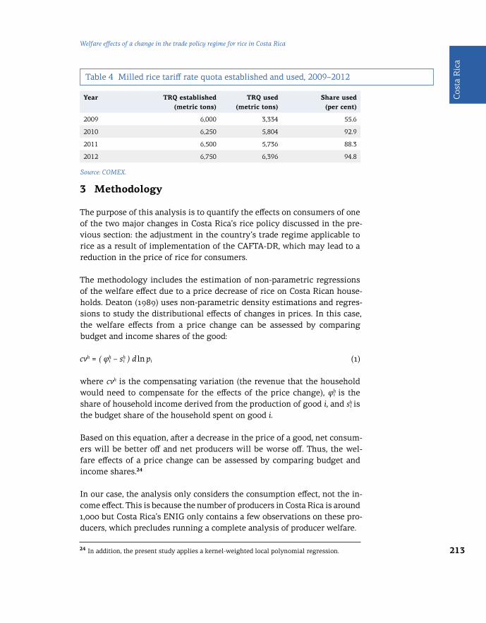
213
Cos
ta R
ica
Welfare effects of a change in the trade policy regime for rice in Costa Rica
Table 4 Milled rice tariff rate quota established and used, 2009–2012
Source: COMEX.
Year TRQ established(metric tons)
TRQ used(metric tons)
Share used (per cent)
2009 6,000 3,334 55.6
2010 6,250 5,804 92.9
2011 6,500 5,736 88.3
2012 6,750 6,396 94.8
3 Methodology
The purpose of this analysis is to quantify the effects on consumers of one of the two major changes in Costa Rica’s rice policy discussed in the pre-vious section: the adjustment in the country’s trade regime applicable to rice as a result of implementation of the CAFTA-DR, which may lead to a reduction in the price of rice for consumers.
The methodology includes the estimation of non-parametric regressions of the welfare effect due to a price decrease of rice on Costa Rican house-holds. Deaton (1989) uses non-parametric density estimations and regres-sions to study the distributional effects of changes in prices. In this case, the welfare effects from a price change can be assessed by comparing budget and income shares of the good:
cvh = ( φhi – sh
i ) d ln pi (1)
where cvh is the compensating variation (the revenue that the household would need to compensate for the effects of the price change), φh
i is the share of household income derived from the production of good i, and sh
i is the budget share of the household spent on good i.
Based on this equation, after a decrease in the price of a good, net consum-ers will be better off and net producers will be worse off. Thus, the wel-fare effects of a price change can be assessed by comparing budget and income shares.24
In our case, the analysis only considers the consumption effect, not the in-come effect. This is because the number of producers in Costa Rica is around 1,000 but Costa Rica’s ENIG only contains a few observations on these pro-ducers, which precludes running a complete analysis of producer welfare.
24 In addition, the present study applies a kernel-weighted local polynomial regression.

214
Trade policies, household welfare and poverty alleviation
Costa Rica’s case is different from countries such as Madagascar, for ex-ample, which in its 2001 household survey reported almost 7,500 observa-tions regarding rice production out of a total number of 11,781 households. For Costa Rica, the assumption is that, on average, households are net con-sumers of rice, as rice constitutes a basic element of the daily diet, and that the net effect of a decrease in the price of rice will consequently be an in-crease in welfare.
Our results reflect only partially the effect of price changes of rice on household welfare. In addition to consumption effects, there are other channels for the impact of price changes on welfare. For example, it may be important to address the issue of workers in the rice (and rice-relat-ed) sectors, since this source of income may be substantial in parts of the country. In this case, the lack of data prevents incorporating this issue into the estimates, but it is nevertheless important to be aware of these other channels through which price changes can affect welfare.
In a study of the welfare effects of Argentina joining the Common Market of the South (MERCOSUR), Porto (2006) affirmed that the first-order ar-gument omits dynamic household responses, and that consumers may re-spond, for example, by substituting more expensive goods with cheaper ones. In rural areas, farmers may increase agricultural production, farm employment and wages, and purchases of inputs and services in local mar-kets. Consequently, the net position of the household becomes endoge-nous: sufficiently large consumption and income responses may cause an ex-ante net consumer to become an ex-post net producer, thus benefiting from the price increase. Furthermore, according to Porto (2010), first-order effects omit the response of labour markets. Many households earn some of their living from wages. If wages depend on the prices of the goods af-fected by the trade reforms, then these mechanisms should be incorporat-ed when classifying households as net producers or net consumers. Other variables to consider are the integration or segmentation of labour mar-kets and the presence of spillovers and linkages. The way labour markets function may also depend on factors such as labour market regulations, la-bour laws and the flexibility to hire and fire workers, and migration costs.
Several authors have presented household models that include labour in-come effects occurring through other channels. For example, in a study on Cambodia, Soloaga (2005) relied heavily on defining the poor in terms of patterns of expenditure and sources of income (ordered by deciles of adult equivalent per capita expenditure) and then on describing their main sources of income. Each household has different endowments (e.g. differ-ent quality of land and different numbers of skilled and unskilled workers)

215
Cos
ta R
ica
Welfare effects of a change in the trade policy regime for rice in Costa Rica
that generate income. Also, each household has different patterns of ex-penditure (e.g. food and non-food expenditure). Soloaga (2005) found that the changes in prices and quantities that would be observed under the baseline scenario of implementation of the Doha Development Agenda would only have a marginal impact on Cambodia’s poor. Meanwhile, under a more ambitious implementation of the agenda, the changes in interna-tional prices coupled with the elimination of all Cambodian tariffs would produce gains of about 7.5 per cent of per capita consumption on average.
McCulloch et al. (2001) provided an analytical framework for understand-ing the linkages between trade liberalization and poverty at the household level. They considered a number of potential generalizations related to the basic view of households, including the following:
• Households can provide several forms of labour (e.g. skilled and un-skilled), so their endowments in this regard and the different wages they command need to be considered.
• Working on and off the farm may not be perfect substitutes for house-hold members (travel costs for off-farm working) and the farm may be better served by family than by non-family labour (perhaps because non-family labour needs to be monitored more than a family member).Thus, the (implicit) “wage” paid to family members may be different from the wage paid to those outside the family, even for the same task.
• It is necessary to incorporate some assumptions about how households allocate their time across the many different activities in which they are involved. Poor households typically earn income in a wide variety of ways, and the allocation of their time to these different activities may change significantly with changes in trade policy.
• Some jobs may only be available for a fixed number of hours per day. Thus, if trade policy affects employment by increasing the amount of time that individuals work, it could have significant effects on poverty.
Several other authors have also examined the link between trade and pov-erty. Topalova (2010) used the case of the Indian trade liberalization in 1991 to measure the impact of trade liberalization on poverty and to examine the mechanisms underpinning this impact. McCaig (2011) analysed the ef-fects of increased United States market access on poverty in Viet Nam and found that poverty fell faster in provinces that experienced the largest tar-iff cuts. Goldberg and Pavcnik (2005) investigated the relationship between protection and industry wage premiums in Colombia. The authors relate

216
Trade policies, household welfare and poverty alleviation
wage premiums to trade policy in an empirical framework that accounts for the political economy of trade protection. Goldberg and Pavcnik (2004) reviewed country case studies that analyse micro data from household or plant-level surveys and establish certain patterns that seem common across countries and trade liberalization episodes, and that may be inform-ative with regard to how developing countries adjust to trade reforms.
The analysis of the decrease in rice prices is based on the reduction of im-port tariffs due to the application of the CAFTA-DR. Welfare effects under three scenarios will be analysed, each related to a particular tariff liberal-ization phase (2015, 2020, and 2025), based on the implementation of the CAFTA-DR’s phasing-out process.
Since we assume a perfect pass-through of tariff reductions, the results here are an upper-bound estimate of the benefits of the tariff phasing-out under the CAFTA-DR. In this sense, the estimation of the pass-through ef-fect for rice may be difficult because there are factors that influence the in-ternal price and that are not easy to measure or quantify, such as political decisions and the degree of integration and competition regarding mar-kets. Also, international prices may not reflect or accurately explain the evolution of internal rice prices in Costa Rica, as prices paid to producers are based on a cost structure that includes elements such as the value of inputs used in production.
The regressions will be run at the national level, but also disaggregated at the following levels: (a) urban versus rural households, (b) region, (c) edu-cation level of the head of the household, and (d) household size.
The results obtained from the non-parametric regressions across the dif-ferent characteristics of households and their per capita consumption lev-el will be particularly useful in terms of determining how an import tariff phase-out process may affect consumers
3.1 Definition of the scenarios: Estimate of the welfare effect from a decrease in the price of rice
The scenarios used in this study were defined based on the estimate of a weighted average tariff for the importation of rice under the CAFTA-DR phasing-out schedule and quotas for rice.25 The period of analysis starts in 2009, when the CAFTA-DR entered into force in Costa Rica, and ends in 2025, when the phasing-out period for paddy and milled rice will be completed.26

217
Cos
ta R
ica
Welfare effects of a change in the trade policy regime for rice in Costa Rica
25 These simulations include paddy, milled and pre-cooked rice. The weights used are based on the total imported volume of rice. Complete pass-through is a reasonable assumption in our case, as the domestic market for rice is influenced by political decisions that may be arbitrary and, as a result, difficult to reflect or quantify in the estimation of the pass-through. 26 Costa Rica’s import data for 2009–2012 are available at the 10-digit level of disaggregation (national tariff classification). 27 Although the best way to justify complete pass-through assumption is by assigning each tariff change to the particular good in household expenditure, in our analysis this was not possible because the rice classification in Costa Rica’s 2004 ENIG is different from the one in international trade statistics (based on the Harmonized System). Therefore, in order to address this limitation, we proceeded by establishing an “overall weighted average” obtained from tariff changes, which was then applied to the share of households’ total expenditure on rice. Rice flour is not defined as an individual product according to the 2004 survey, and it was not considered for the estimation of the scenarios.
It is assumed that the import quotas defined in the CAFTA-DR for pad-dy and milled rice will be completely used during the years ahead (2013–2024). The estimated share of intra-quota CAFTA-DR imports of rice in total rice imports from the United States for 2009–2012 was 69 per cent for paddy rice and 80 per cent for milled rice. These shares were applied to the respective CAFTA-DR quota volumes for each year from 2013 to 2024 in order to define the extra-quota volumes and, as a result, the total esti-mated imports of paddy and milled rice from the United States. Note that almost all of Costa Rica’s paddy rice imports come from the United States.
For milled rice imports from the rest of the world (aside from the United States), the volume forecast for 2013 was obtained by multiplying the an-nual average growth rate for rice consumption in Costa Rica during the 2001–2002 and 2011–2012 harvest seasons (2.03 per cent) by the average imported volume during 2009–2012 from each of the countries of origin. For countries other than the United States, the same growth rate (2.03 per cent) was applied for the estimation of 2013–2024 milled rice imports.
Welfare evaluations are done for four points in time: a baseline scenario based on the data from 2009–2012, which represents the first four years of CAFTA-DR implementation in Costa Rica; a second scenario in 2015, the last year in which the MFN tariff will be applied to out-of-quota CAFTA-DR im-ports from the United States; a third scenario in 2020, when pre-cooked rice imports from the United States will enjoy duty-free access; and the final sce-nario in 2025, when all rice imports from the United States will be duty-free.
As shown in Table 5, the overall weighted average tariff for rice will move from 12.1 per cent in 2009–2012 to 6.6 per cent in 2020. In 2025, the overall weighted tariff will be zero. This general average tariff can be used to define a price change.27 As a result, the estimated price change for each of the sce-narios in relation to the baseline years (2009–2012) will be the following:

218
Trade policies, household welfare and poverty alleviation
• 2025 scenario: –12.1 per cent • 2020 scenario: –5.52 per cent• 2015 scenario: –1.51 per cent
For pre-cooked rice, the average weighted tariff for each of the years from 2013–2024 results from the multiplication of the applied tariff in each year by the share that each exporting country represented in the total volume imported by Costa Rica in 2012. The base year 2012 for the exporting coun-try’s share was chosen because that year shows a better representation of how imports would be distributed by country of origin during the follow-ing years. In 2012, the United States accounted for the highest share of Costa Rica’s total imports of pre-cooked rice (50.1 per cent).
Source: Author’s calculations, based on data from the Central Bank of Costa Rica and COMEX. Notes: Figures in the table are forecasts. Annex 3 contains more information about weights, average tariffs and assumptions for the estimate of the weighted average tariff. The column entitled “Weight” indicates the share of imports of each type of rice in the volume of total rice imports. The column entitled “Weighted average tariff (by product)” gives the trade-weighted aver-age tariff for each rice category as well as the average tariff applied to rice weighted according to the importance of each rice category in rice imports.
Table 5 Weighted average tariff for rice imports to Costa Rica, 2009–2012, 2015 and 2020 (per cent)
Rice product Weight Weighted average tariff (by product)
2009-2012
Paddy 83.4 12.3
Milled 13.2 11.4
Pre-cooked 3.4 9.3
Total 100.0 12.1
2015
Paddy 81.8 10.9
Milled 14.8 10.0
Pre-cooked 3.4 6.0
Total 100.0 10.6
2020
Paddy 81.1 6.5
Milled 15.5 8.3
Pre-cooked 3.4 0.0
Total 100.0 6.6
28 The fact that the expenditure structure of the households will not change is established as a ceteris paribus assumption for simplicity purposes.

219
Cos
ta R
ica
Welfare effects of a change in the trade policy regime for rice in Costa Rica
3.2 Data access and availability
This study uses Costa Rica’s 2004 National Income and Expenditure Survey, which includes three databases. The first covers variables relat-ed to the characteristics of household members, such as education level, employment, income, and transfers. A second database includes variables linked to household characteristics, such as the type of dwelling, number of rooms, and availability of appliances, domestic workers, persons who receive government aid, household incomes, and other characteristics. A third database has a more disaggregated classification of household ex-penditures by specific products. For example, this database provides the share of household expenditure on rice in which all four types of rice are considered as a single product.
The fact that the survey dates to 2004 is not a limitation because tariff conditions for rice have not changed. Nor has there been much change in the composition of the poorest quintile. This study thus assumes that the structure of household expenditure has not changed between 2004 and the following years, including the baseline years of 2009–2012 and the phas-ing-out scenarios years (2015, 2020, and 2025).28
4 Welfare estimates for Costa Rica’s households from a decrease in the price of rice
4.1 Estimates at the national, urban and rural levels
Figures 7–10 show welfare gains from the decrease in the price of rice in the years ahead, assuming that the reduction in import tariffs will be com-pletely transmitted to local prices.
Welfare gains are expected to be positive during those years as tariffs de-crease during the phasing-out process. As expected, welfare gains will be-come relatively more significant for poor households, particularly for poor urban households that are expected to benefit the most from a price de-crease in rice. Their welfare gains may account for more than 0.05 per cent of their initial consumption level in 2015, around 0.30 per cent in 2020, and close to 1 per cent for the 2025 full tariff liberalization scenario (Figure 7).29
29 Further research could assess welfare effects by showing estimates by deciles or centiles of income distribution (Nicita, 2004). The reason is that non-parametric regressions are local regressions by nature and, as such, they do not indicate the income percentile of households at each point of the estimated curve.

220
Trade policies, household welfare and poverty alleviation
Figure 7 Welfare changes in the 2025, 2020 and 2015 scenarios compared to 2009–2012, at the national level and by urban and rural areas
― National
― Urban
Rural
0
.2
.4
.6
.8
1
8 10 12 14 16
Wel
fare
cha
nge
Log per capita expenditure
2025
0
.1
.2
.3
.4
.5
8 10 12 14 16
Wel
fare
cha
nge
Log per capita expenditure
2020― National
― Urban
Rural

221
Cos
ta R
ica
Welfare effects of a change in the trade policy regime for rice in Costa Rica
Source: Author’s calculations, based on the 2004 ENIG.
Middle-income households will also benefit from a reduction in rice pric-es. For example, under the 2015 scenario, welfare gains for this group of households will reach around 0.04 per cent; the 2020 scenario shows a benefit close to 0.15 per cent; and the 2025 scenario shows welfare gains of around 0.30 per cent. Welfare gains for the richest households are negligi-ble, a fact that is consistent with Engel’s Law, as the share of rice in their budget is relatively small compared to low-income households. Also, the wealthiest population can afford a more diversified diet, away from rice.
A complementary way to assess welfare effects from a reduction in the price of rice is by comparing the average welfare effect according to de-ciles of income distribution. In this way, and assuming that the reduction in import tariffs will be completely transmitted to local prices, Table 6 shows that, at the national level, welfare effects will be more relevant in the poorest deciles. For example, households in the first decile will show, under the 2025 scenario, a 0.66 per cent welfare increase from their initial consumption level. This is a result that complements Figure 7, as lower-in-come households will enjoy higher welfare increases due to a reduction in rice prices.
― National
― Urban
Rural
0
.05
.1
0.15
8 10 12 14 16
Wel
fare
cha
nge
Log per capita expenditure
2015

222
Trade policies, household welfare and poverty alleviation
4.2 Welfare effects by region
With regard to welfare effects by region, all regions show a common down-ward tendency as household income increases. Under the 2025 scenario, the region that shows the highest welfare increase for the poorest seg-ments of the population is the Chorotega Region, followed by the Huetar Atlántica and Brunca Regions (Figure 8).30 In these cases, welfare increases for poor households from a complete tariff liberalization of rice may reach, on average, 0.50 per cent or more from the baseline consumption level.
Source: Author’s calculations, based on the 2004 ENIG.
Source: Author’s calculations, based on the 2004 ENIG.
Figure 8 Welfare change in the 2025 scenario compared to 2009–2012, by region
30 Figure A1.1 in Annex 1 shows the results for the 2015 and 2020 scenarios. 31 Figure A1.2 in Annex 1 shows the results for the 2015 and 2020 scenarios. 32 Large households with more children may dedicate a larger budget share to rice.
Wel
fare
cha
nge
Log per capita expenditure
8
0
.2
.4
.6
.8
10 12 14 16
― Central
― Pacífico Central
― Huetar Atlántica
― Chorotega
Brunca
Huetar Norte
Decile Scenario
2025 2020 2015
1 0.66 0.30 0.08
2 0.38 0.17 0.05
3 0.27 0.12 0.03
4 0.22 0.10 0.03
5 0.17 0.08 0.02
Decile Scenario
2025 2020 2015
6 0.17 0.08 0.02
7 0.13 0.06 0.02
8 0.08 0.03 0.01
9 0.05 0.02 0.01
10 0.02 0.01 0.00
Table 6 Welfare changes in the 2025, 2020 and 2015 scenarios at the national level, by deciles of income distribution (per cent)

223
Cos
ta R
ica
Welfare effects of a change in the trade policy regime for rice in Costa Rica
The Chorotega Region, as well as the Huetar Atlántica and Brunca Regions, have consistently had high poverty levels. For example, according to the average poverty incidence for 2010–2012, the share of the population liv-ing in poverty was 34.1 per cent in the Brunca Region, 32.9 per cent in Chorotega, and 27.9 per cent in Huetar Atlántica.
Figure 8 shows that gains are larger for these poor regions in Costa Rica. In contrast, the Central Region shows the lowest welfare gains from a price decrease in rice (except for the poorest households), probably due to the fact that this region has recorded the lowest poverty incidence lev-els in Costa Rica. However, we must be cautious about interpreting this regional disaggregation, since the Chorotega Region is at the same time the largest producer of rice, and the present study does not consider in-come effects.
Furthermore, Figure 8 shows relatively large differences in the welfare effects across regions, conditional on per capita expenditure. This means that a poor household with the same per capita expenditure, on aver-age, benefits more in the Chorotega Region than in the Brunca or Central Region. The differences in the expenditure share of rice across regions (e.g. due to differences in tastes) might be the underlying reason for these dif-ferent effects. For instance, according to the 2004 survey, households with the same per capita expenditure dedicated 3.6 per cent of their average budget to rice in the Chorotega Region, followed by the Huetar Atlántica Region (3.1 per cent), and the Brunca Region (2.9 per cent), while they only spent, on average, 1.1 per cent of their budget on rice in the Central Region. Consequently, the increase in welfare resulting from a rice price decrease is, on average, more pronounced for households in regions with a higher share of rice in total expenditure.
4.3 Welfare effects according to household size
Figure 9 shows the welfare effects of a reduction in rice prices based on the number of household members (household size).31 The 2025 scenario shows that the poorest and largest households, with six or more members, may enjoy the most significant welfare effects.32 According to the 2011 cen-sus, the districts at the national level with a higher incidence of resource gaps, based on the unmet basic needs approach, are those that have a larg-er average size of households (4 members per household compared to 3.5 members per household at the country level) (Méndez and Bravo, 2011). Unmet basic needs refer to the housing quality, overcrowding, electrici-ty, health, physical infrastructure, consumption capacity, primary and sec-ondary school attendance and school achievement.

224
Trade policies, household welfare and poverty alleviation
Differences in the welfare effects on households, as shown in Figure 9, can be explained by the disparities in the expenditure share of rice for different household sizes. According to the 2004 survey, in households with six or more members, rice represented, on average, 2.7 per cent of the household budget, while for households with two to five members the share was 1.6 per cent. In contrast, households composed of one member spent, on aver-age, 1.4 per cent of their budget on rice. In other words, larger households spent, on average, a higher share of their budget on rice.
Source: Author’s calculations, based on the 2004 ENIG.
Figure 9 Welfare change in the 2025 scenario compared to 2009–2012, by household size
― National
1 member
― 2–5 members
6 or more members
Wel
fare
cha
nge
Log per capita expenditure8
0
.2
.4
.6
.8
10 12 14 16
33 Figure A1.3 in Annex 1 shows the results for the 2015 and 2020 scenarios. 34 Figures 7–10 remove extreme values. Fitted values from non-parametric regressions could be problematic when we are interested in the extremes, as they may have few obser- vations to perform the regressions and thus produce imprecise estimations. For example, the dataset contains six observations for secondary education with log per capita < 9.5 (representing 0.6 per cent of the total number of observations for secondary education). Furthermore, in Figure 10, the national curve differs from the previous figure due to the different limits applied to remove potential extreme observations in the data. 35 These four regions were Chorotega, Brunca, Huetar Atlántica, and Huetar Norte.
A possible explanation for the differences in rice consumption across house-holds is that households with only one member are less likely to cook and eat at home. Instead, they may go to restaurants or eat elsewhere. On the other hand, larger households are more likely to benefit from economies of scale when cooking and eating at home. According to the survey, sin-gle-member households spend on average 7.2 per cent of their budget on consumption of food and beverages prepared outside the home, compared to 5.4 per cent, on average, for households with two or more members.

225
Cos
ta R
ica
Welfare effects of a change in the trade policy regime for rice in Costa Rica
Source: Author’s calculations, based on the 2004 ENIG.
Figure 10 Welfare change in the 2025 scenario compared to 2009–2012, by education level
4.4 Education level of the household head
When comparing the education level of the household head, those who have not received an education experience the largest increase in welfare from a reduction in the price of rice (Figure 10).33 Also, conditional on per capi-ta household expenditure, their budget share spent on rice is higher.34 For example, according to the survey, households whose head has no education display the highest rice expenditure budget share (3.6 per cent), followed by households whose head has an elementary education (2.4 per cent), second-ary education (1 per cent), or university education (0.4 per cent).
As the education level of the household head decreases, the average wel-fare gain for households will progressively increase. Given that we are controlling for income, we do not have an a priori explanation for these dif-ferences. Probably, the education variable is correlated with another var-iable. The survey shows that in four of the six regions of Costa Rica, the share of household heads with no education or with elementary education (completed or not) reached the highest levels, with more than 65 per cent in each region.35 The same four regions have the highest share of rice ex-penditure, as described in Section 4.2.
This classification thus serves as another tool to identify the profile of house-holds that will obtain the largest gains from a decrease in the price of rice. For example, welfare gains for households whose head has no education will be double those of households whose head has a secondary education.
Wel
fare
cha
nge
Log per capita expenditure
10
0
.1
.2
.3
.4
11 12 13 1615
― National
― University
Secondary
― Elementary
No education
226
Trade policies, household welfare and poverty alleviation
5 Conclusions, policy recommendations and discussion
5.1 Conclusions
The rice market in Costa Rica has several distinct features. First, rice is an essential staple in the Costa Rican diet, particularly for the poorest seg-ments of the population. Second, rice is produced in the country, but lo-cal production does not satisfy local demand. Third, rice has been subject to several policy measures targeting both local production and imports. The performance requirement for the importation of paddy rice from the United States, for instance, has benefited those producers that are verti-cally integrated (i.e. those that manage both the production and milling of rice). Fourth, the price-fixing mechanism has increased prices of paddy rice paid to local producers to double that of international prices. Consequently, Costa Rican consumers are paying a high price for a key commodity in their daily basket, the consumption of which is even more important for low-income households. Costa Rica’s current rice policies have not been successful in increasing productivity, reducing prices for consumers, or improving conditions for small farmers. It is the large producers who re-ceive the rents from the use of the performance requirement for paddy rice imports. Also, due to the price-fixing mechanism, Costa Rica is in breach of its WTO commitments, as the amount of distorting support received by producers in recent years has exceeded by more than five times the maxi-mum amount allowed under those commitments.
At the same time, the trade regime for rice imports is changing as a result of the entry into force of the CAFTA-DR: the phasing-out process for out-of-quota import tariffs will begin in 2016, and unlimited duty-free access for imports from the United States is scheduled for 2025. The CAFTA-DR thus may be an opportunity to effectively reduce rice prices in the domes-tic market and in doing so improve the welfare of consumers.
This study analysed the effects of a price decrease of rice on consumers by estimating a reduction in prices for rice imports at several points in time (2015, 2020, and 2025). As a starting point, the study established a baseline scenario that considered the weighted import tariffs on rice for the period 2009–2012. The database used was Costa Rica’s 2004 National Income and Expenditure Survey, and it was assumed that the expenditure structure of the households would not change.
By applying non-parametric regressions, the study arrived at several re-sults. As expected, the poorest will benefit the most from a decrease in

227
Cos
ta R
ica
Welfare effects of a change in the trade policy regime for rice in Costa Rica
the price of rice. In the 2025 scenario with duty-free access for imports from the United States, the poorest urban households may record a wel-fare increase close to 1 per cent from the baseline period consumption lev-el (2009–2012). Other results have shown the links between welfare gains and characteristics such as the area and region where households are lo-cated, household size and the education of the household head.
For comparison, we considered the results of Porto (2006), who analysed the welfare effects of Argentina joining the MERCOSUR, assuming that price changes are given by tariff changes. That study calculated the budget shares for these products, and estimated the welfare effects by multiply-ing these shares by the price changes. In that case, the total consumption effect was positive for almost all households, except the poorest ones. By adding the consumption effects of traded and non-traded goods, the total consumption effect increased monotonically with the level of livelihood, with changes ranging from around –0.2 per cent to over 2.2 per cent of ini-tial expenditure. The richer the household, the larger was the welfare gain.
The results of our study have shown that households in the poorest regions of the country will enjoy a greater increase in welfare as a result of price reductions in rice. Poorest households in urban areas will gain the most. Moreover, households with six or more members will greatly benefit, as will households whose head has no education. However, if the decrease in import tariffs for rice from the application of the CAFTA-DR is not reflected in a price reduction for this product in the domestic market, then the sub-sequent welfare gains for the poor sectors of the population will be missed.
As mentioned earlier, this study has only included consumption effects, not income effects. It has not considered any general equilibrium effect coming from reductions in employment in the rice sector. It could be the case that although many households are net rice consumers, and as such benefit from price reductions, they are also affected by negative labour outcomes derived from losses in domestic production. Furthermore, we assume a perfect pass-through for tariff reductions, and, therefore, results here are an upper-bound estimate of the benefits of the phasing-out of tariffs under the CAFTA-DR.
This study is expected to be a starting point from which other analyses in Costa Rica can be performed using micro data. At the time of our analysis, the National Institute of Statistics and Census of Costa Rica was collecting information from households for preparation of the 2012–2013 National Income and Expenditure Survey. This database will provide up-to-date in-formation for new studies regarding the quantification of welfare effects of trade policies.

228
Trade policies, household welfare and poverty alleviation
5.2 Policy recommendations
The results of this study have shown that poor households in Costa Rica will likely be the segment of the population to benefit most from a reduc-tion in the price of rice. In this sense, the phasing-out process scheduled in the CAFTA-DR may be an opportunity to effectively reduce rice prices in the domestic market.
For this to take place, the institutions in charge of defending the interests of consumers, as well as those that supervise the functioning of the do-mestic market, must develop an active stance towards surveillance of price behaviour for the imported product, especially after 2016. During 2009–2012, the weighted average import tariff for rice was 12.1 per cent; this percentage therefore represents the estimated reduction in local prices of rice in 2025 (the year when imports of milled and paddy rice will enjoy du-ty-free access) compared to the prices of 2009–2012.
This study has kept the international price at its current level. It is impor-tant to take into consideration the fact that international prices can change in the future. However, this study did not aim to perform forecasts with re-gard to price levels.
As a result of Costa Rica’s price-fixing mechanism, there is no transmis-sion of international prices of rice to domestic prices. If the internation-al price falls, then the domestic price does not move, which is equivalent to zero transmission. In the domestic market, if the price to the produc-er increases by virtue of a decree, then consumer prices rise at a rate giv-en by the margins.36
The implementation of the phasing-out process in the CAFTA-DR will pro-gressively reduce the relevance of the performance requirement for paddy rice imports from the United States, as well as the import quota, since the out-of-quota import tariff will move closer to zero. This means that indus-tries will not need to purchase domestic paddy rice in order to be able to import duty-free from the United States. Large producers, which are also millers, may have an incentive to import most of the paddy rice they will process, depending on how profitable producing locally or importing rice will become. If large producers have a better business opportunity by im-porting most of their rice and reducing their own production, this may re-quire an active policy of stocks and safety nets to address international price spikes.
36 Conceptually, then, this could not be called transmission.

229
Cos
ta R
ica
Welfare effects of a change in the trade policy regime for rice in Costa Rica
37 As mentioned earlier, we must be cautious in interpreting this regional disaggregation because the Chorotega Region is also the largest producer of rice, and our study did not consider income effects.
The reduction of the price of rice is a pro-poor measure. The results pre-sented in this study have identified with a greater level of detail which population groups may obtain the highest welfare gains from such a re-duction: poor households living in urban areas, households whose head has a lower education level, large households, and households living in the Chorotega, Huetar Atlántica, and Brunca Regions.37 These outcomes explain why the CAFTA-DR is an opportunity for Costa Rican households, in particular the poorest, to get better access to affordably priced rice.
5.3 Discussion
With the arrival of the CAFTA-DR, the local rice sector faces the chal-lenge of increasing its competitiveness, including: (a) productivity, which has decreased in recent years; (b) capacity-building for rice producers; (c) improved and cheaper access to inputs, a growing concern for the sector; and (d) strengthening of credit mechanisms, which is specifically crucial for small producers who may require this kind of assistance. In this sense, Decree 37699-MEIC defines a coordinated programme of work between the government and the rice sector to increase competitiveness, facilitate access to credit, and achieve an effective reduction in the costs of inputs such as agrochemicals and seeds.
Costa Rica has to continue its efforts to comply with its commitments to the WTO. A continuous dialogue needs to take place between producers, millers and the government in order to enhance productivity levels, avoid the need to apply trade-distorting policies, and prevent a loss in welfare for consum-ers. The CAFTA-DR might serve as an automatic price control mechanism resulting in rice imports becoming progressively cheaper. Local producers may then be pushed to reduce their prices to avoid losing their market share.
The possibility of applying price fixing should not be politicized, even if Article 5 of the Law for Promotion of Competition and Effective Consumer Protection (Law No. 7472) allows the government to regulate the prices of goods and services in exceptional situations. This measure needs to be ap-plied only temporarily, and the need for its application has to be properly established and justified.
It is important to consider that this study is an empirical exercise regard-ing the estimation of a possible price decrease due to the application of the

230
Trade policies, household welfare and poverty alleviation
phasing-out schedule of the CAFTA-DR. However, the real context is com-plex and includes other elements such as policy decisions and the organ-ization of the market. For this reason, the analysis may be considered as a first step towards assessing the welfare gains for households from a de-crease in the price of rice. In addition, this research considered only con-sumption effects, due to the lack of observations for rice producers in Costa Rica’s 2004 National Income and Expenditure Survey. It also did not in-clude the consequences of a price decrease of rice for producers.
Finally, the study agrees with Arroyo et al. (2013) that the current price-fix-ing mechanism is neither increasing productivity nor improving consum-er access to affordable rice. Among the alternative policies that may thus be proposed are to:
• Continue using the price-fixing mechanism while ensuring that the to-tal subsidy to rice farmers does not exceed Costa Rica’s WTO commit-ments, and focus the support on small producers.
• Revise the legal scope of the current pricing mechanism to include alternatives that do not breach the commitments at the multilater-al level (so-called “green box” measures in the WTO Agreement on Agriculture). The heterogeneity of the sector may be considered, as sup-port should be more focused on small producers, who particularly need-to increase productivity and competitiveness. Measures may include extension services (such as research, training, and pest and disease con-trol), as well as direct payments to producers, provided that such pay-ments are decoupled from production.
Finally, and importantly, whatever pricing mechanism is ultimately imple-mented, it must consider the potential impact on consumers.
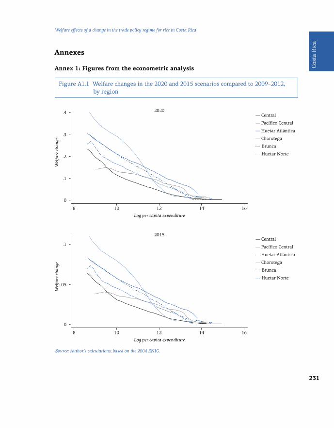
231
Cos
ta R
ica
Welfare effects of a change in the trade policy regime for rice in Costa Rica
Annexes
Annex 1: Figures from the econometric analysis
Figure A1.1 Welfare changes in the 2020 and 2015 scenarios compared to 2009–2012, by region
Source: Author’s calculations, based on the 2004 ENIG.
Wel
fare
cha
nge
Wel
fare
cha
nge
Log per capita expenditure
Log per capita expenditure
8
8
0
0
.1
.2
.05
.3
.4
.1
10
10
12
12
14
14
16
16
― Central
― Pacífico Central
― Huetar Atlántica
― Chorotega
Brunca
Huetar Norte
― Central
― Pacífico Central
― Huetar Atlántica
― Chorotega
Brunca
Huetar Norte
2020
2015

232
Trade policies, household welfare and poverty alleviation
Figure A1.2 Welfare changes in the 2020 and 2015 scenarios compared to 2009–2012, by household size
Wel
fare
cha
nge
Log per capita expenditure
8
0
.1
.2
.3
.4
10 12 14 16
2020
Wel
fare
cha
nge
Log per capita expenditure8
0
.04
.02
.06
.08
.1
10 12 14 16
2015
Source: Author’s calculations, based on the 2004 ENIG.
― National
1 member
― 2–5 members
6 or more members
― National
1 member
― 2–5 members
6 or more members

233
Cos
ta R
ica
Welfare effects of a change in the trade policy regime for rice in Costa Rica
Figure A1.3 Welfare changes in the 2020 and 2015 scenarios compared to 2009–2012, by education level
2020
Source: Author’s calculations, based on the 2004 ENIG.
Wel
fare
cha
nge
Log per capita expenditure
10
0
.05
.1
.15
.2
11 12 13 1615
Wel
fare
cha
nge
Log per capita expenditure
10
0
.01
.03
.02
.04
.05
11 12 13 1615
2015
― National
― University
Secondary
― Elementary
No education
― National
― University
Secondary
― Elementary
No education

234
Trade policies, household welfare and poverty alleviation
Annex 2: Facts about the domestic rice market in Costa Rica
Table A2.1 Imports and national production relative to domestic supply of milled equivalent rice in Costa Rica, 1995–2009 (per cent)
Table A2.2 Official fixed price to rice producers and national production that benefited from the price-fixing regime, 1995–2010
Year Imports/Domestic consumption
National production/Domestic consumption
1995 32.0 70.9
1996 30.2 73.1
1997 30.6 75.5
1998 38.3 66.2
1999 24.1 80.2
2000 20.5 81.7
2001 28.7 77.3
2002 35.6 66.4
2003 47.2 54.3
2004 46.6 55.3
2005 58.4 43.1
2006 56.3 44.1
2007 52.3 49.7
2008 34.2 70.6
2009 32.8 69.6
Average 37.9 65.2
Source: COMEX.Note: Since domestic supply = imports + national production – exports, the sum of imports and national production in each row may not equal 100.
Year Official fixed price(USD per metric ton)*
National production(metric tons)
1995 260.9 164,866
1996 267.6 212,873
1997 280.7 223,676
1998 280.2 215,099
1999 271.0 264,317
2000 267.3 266,422

235
Cos
ta R
ica
Welfare effects of a change in the trade policy regime for rice in Costa Rica
Source: COMEX, based on data from CONARROZ.* Based on figures provided by Costa Rica in notifications to the WTO Committee on Agriculture.**According to 2010–2011 harvest figures from CONARROZ.
Year Official fixed price(USD per metric ton)*
National production(metric tons)
2001 257.8 216,700
2002 248.2 189,689
2003 259.6 183,497
2004 258.3 197,211
2005 271.7 183,251
2006 305.5 175’775
2007 353.4 179,729
2008 506.7 220,870
2009 581.3 256,612
2010 633.4 290,475**
Annex 3: Average tariffs and weights applied to intra-CAFTA-DR imports and to non-CAFTA-DR imports38
Pre-cooked rice
Weights applied for 2009–2012 are based on the total sum of the share of imported volume in each year, multiplied by the applied tariff, for each im-port partner. Weights estimated for 2015 are based on the share of imported volume, by import partners, in 2012 (Table A3.1).39 For 2020, it is assumed that all pre-cooked rice will be imported duty-free from the United States.
38 Sources of information for this Annex include the CAFTA-DR phasing-out schedule for Costa Rica, trade statistics from the Central Bank of Costa Rica, and Costa Rica’s MFN applied tariffs from the WTO. 39 The same weights are applied throughout 2013–2019.

236
Trade policies, household welfare and poverty alleviation
Table A3.1 Weighted average tariff for pre-cooked rice imports to Costa Rica, 2009–2012 and 2015 (per cent)
United States
El Salvador Uruguay Total weighted average tariff
2009–2012
Weight 2 < w < 50 17 < w < 47 23 < w < 719.3*Applied tariff 8 < at < 11 0.0 15.0
Weighted average tariff 2.0 0.0 6.3
2015
Weight 50.1 26.8 23.16.0Applied tariff 5.0 0.0 15.0
Weighted average tariff 2.5 0.0 3.5
Source: Author’s calculations.Note: w stands for weight and at stands for applied tariff.
*During 2009–2011, Costa Rica imported pre-cooked rice from other countries that are not included in this table, which is why the total weighted average tariff (9.3 per cent) does not coincide with the sum of the weighted average tariffs of the United States and Uruguay (8.3 per cent).
Source: Author, based on Costa Rica’s phasing-out schedule in the CAFTA-DR.
The CAFTA-DR does not apply tariff rate quotas for pre-cooked rice. The phasing-out process from a 15 per cent base rate is shown in Table A3.2
Table A3.2 Phasing-out of the pre-cooked rice import tariff in the CAFTA-DR (per cent)
Year CAFTA-DR tariff
1 2006 14
2 2007 13
3 2008 12
4 2009 11
5 2010 10
6 2011 9
7 2012 8
8 2013 7
Year CAFTA-DR tariff
9 2014 6
10 2015 5
11 2016 4
12 2017 3
13 2018 2
14 2019 1
15 2020 0

237
Cos
ta R
ica
Welfare effects of a change in the trade policy regime for rice in Costa Rica
Table A3.3 Weighted average tariff for paddy rice imports to Costa Rica, 2009–2012, 2015 and 2020 (per cent)
Source: Author’s calculations.*Imports of paddy rice from El Salvador are duty-free due to the CACM. Annual forecast growth of imports from El Salvador is based on annual growth of rice consumption between 2001–2002 and 2011–2012 crop seasons (2.03 per cent).
Paddy rice
The weights applied in Table A3.3 are based on total imported volume of paddy rice, by import partners, during the period 2009–2012.
Intra-quota CAFTA-DR
Out-of-quota CAFTA-DR
El Salvador* Total weighted
average tariff
2009–2012
Weight 65.4 34.3 0.312.3Applied tariff 0 36 0
Weighted average tariff 0 12.3 0
2015
Weight 68.6 30.3 1.110.9Applied tariff 0 36 0
Weighted average tariff 0 10.9 0
2020
Weight 68.6 30.3 1.16.5Applied tariff 0 21.6 0
Weighted average tariff 0 6.5 0
The following assumptions are made: (a) the CAFTA-DR TRQ is complete-ly used, and (b) 69.4 per cent of imports from the United States are intra- CAFTA-DR quotas (based on the share reported in 2009–2012).
The MFN tariff is 36 per cent, the applied tariff for intra-CAFTA-DR im-ports is zero, and tariffs for out-of-quota CAFTA-DR imports from 2009 to 2025 are specified in Table A3.4.

238
Trade policies, household welfare and poverty alleviation
Table A3.4 Phasing-out of the out-of-quota import tariff for paddy rice in the CAFTA-DR (per cent)
Table A3.5 Share of milled rice imports to Costa Rica, by country of origin, 2009–2012, 2015 and 2020 (per cent)
Year CAFTA-DR out-of-quota tariff
4 2009 36
5 2010 36
6 2011 36
7 2012 36
8 2013 36
9 2014 36
10 2015 36
11 2016 33.1
12 2017 30.2
Source: Author’s calculations, based on Costa Rica’s phasing-out schedule in the CAFTA-DR.
Milled rice
The weights applied in Table A3.5 are based on total imported volume of milled rice, by import partners, during 2009–2012.
Import weights
Country of origin 2009–2012 2015 2020
Argentina* 12.3 10.8 10.5
Brazil* 0.5 0.5 0.4
China* 0.2 0.2 0.2
Ecuador* 0.1 0.1 0.1
El Salvador** 6.7 5.9 5.7
United States intra-quota CAFTA-DR 40.3 47.2 48.3
United States out-of-quota CAFTA-DR 13.1 11.5 11.8
Guatemala** 3.0 2.6 2.5
Guyana* 0.2 0.2 0.2
Nicaragua** 18.5 16.3 15.8
Uruguay* 5.2 4.6 4.5
Total 100.0 100.0 100.0
Source: Author’s calculations.*Imports of milled rice are subject to a 15 per cent MFN import tariff. **Imports of milled rice from El Salvador, Guatemala, and Nicaragua are duty-free due to the CACM.
Year CAFTA-DR out-of-quota tariff
13 2018 27.4
14 2019 24.5
15 2020 21.6
16 2021 17.3
17 2022 13.0
18 2023 8.6
19 2024 4.3
20 2025 0.0

239
Cos
ta R
ica
Welfare effects of a change in the trade policy regime for rice in Costa Rica
The following assumptions are made: (a) the CAFTA-DR TRQ is used; (b) 80.4 per cent of imports from the United States are within the intra-CAF-TA-DR quota (based on the share reported for 2009–2012); and (c) annual forecast growth of imports from countries other than the United States is based on annual growth in rice consumption between the 2001–2002 and 2011–2012 crop seasons (2.03 per cent).
The MFN tariff is 36 per cent, the applied tariff for intra-CAFTA-DR im-ports is zero, and the tariff treatment for out-of-quota CAFTA-DR imports from 2009 to 2025 is the same as that applied to out-of-quota CAFTA-DR imports of paddy rice (as presented previously in this Annex).
As a result, the weighted average tariffs for milled rice are shown in Table A3.6.
Table A3.6 Weighted average tariff for milled rice imports to Costa Rica, 2009–2012, 2015 and 2020 (per cent)
2009–2012 2015 2020
Argentina 4.4 3.9 3.8
Brazil 0.2 0.2 0.2
China 0.1 0.1 0.1
Ecuador 0.0 0.0 0.0
El Salvador 0.0 0.0 0.0
United States intra-quota CAFTA-DR 0.0 0.0 0.0
United States out-of-quota CAFTA-DR 4.7 4.1 2.5
Guatemala 0.0 0.0 0.0
Guyana 0.1 0.1 0.1
Nicaragua 0.0 0.0 0.0
Uruguay 1.9 1.7 1.6
Total 11.4 10.0 8.3
Source: Author’s calculations.
240
Trade policies, household welfare and poverty alleviation
References
Arroyo, N. Lücke, R. and Rivera, L. (2013). Análisis sobre el mecanismo actual para la estimación y determinación de los precios del arroz bajo el contexto de la cadena de comercialización. Final report by the Institute for Economic Sciences Research for the Ministry of Economy, Industry and Commerce, San José.
COMEX, MEIC and Ministry of Agriculture (2010). Incidencia del mecanismo de fijación de precios del arroz sobre el produc-tor, el consumidor y las obligaciones internacionales de Costa Rica. Ministry of Foreign Trade of Costa Rica, San José.
Deaton, A. (1989). “Rice Prices and Income Distribution in Thailand: A Non-Parametric Analysis.” Economic Journal, 99 (395): 1–37.
Goldberg, P. and Pavcnik, N. (2004). “Trade, Inequality, and Poverty: What Do We Know? Evidence from Recent Trade Liberalization Episodes in Developing Countries.” NBER Working Paper No. 10593. National Bureau of Economic Research, Cambridge MA.
Goldberg, P. and Pavcnik, N. (2005). “Trade, Wages, and the Political Economy of Trade Protection: Evidence from the Colombian Trade Reforms.” Journal of International Economics, 66 (1): 75–105.
Jovel Díaz, R. and Díaz Porras, R. (2007). “El sector arrocero en Costa Rica desde la perspectiva de cadenas globales de mercancías.” Revista Centroamericana de Administración Pública, 52–53: 63–95.
McCaig, B. (2011). “Exporting Out of Poverty: Provincial Poverty in Vietnam and U.S. Market Access.” Journal of International Economics, 85 (1): 102–113.
McCulloch, N., Winters, L.A. and Cirera, X. (2001). Trade Liberalization and Poverty: A Handbook. Centre for Economic Policy Research, London.
Méndez, F. and Bravo, O. (2011). “Mapas de pobreza con datos censales.” Presented at the symposium “Costa Rica a la luz del Censo de 2011”. University of Costa Rica, San José, 8–9 November 2012.
Nicita, A. (2004). “Who Benefited from Trade Liberalization in Mexico? Measuring the Effects on Household Welfare.” Policy Research Working Paper No. 3265. World Bank, Washington DC.
Petrecolla, D. (2006). Costa Rica: Agrocadena del arroz. Estudio sectorial de competencia. Final Report by the World Bank and the International Finance Corporation Foreign Investment Advisory Service.
Porto, G. (2006). “Using Survey Data to Assess the Distributional Effects of Trade Policy.” Journal of International Economics, 70 (1): 140–160.
Porto, G. (2010). “On Trade, Prices, and Poverty in Developing Countries.” Mimeo. Policy Research Department, World Bank, Washington DC.
Regional Agriculture Sectoral Committee of the Chorotega Region (2008). Programa Regional de Producción de Alimentos 2008–2010.
SEPSA (2012). Boletín Estadístico Agropecuario #22. Secretaria Ejecutiva de Planificación Sectorial Agropecuaria, San José.
Soloaga, I. (2005). “Cambodia.” Poverty Impacts of Global Trade Reform – Case Studies [online]. Yale Center for the Study of Globalization. Available at: http://www.ycsg.yale.edu/focus/povertyImpact.html.

241
Cos
ta R
ica
Welfare effects of a change in the trade policy regime for rice in Costa Rica
Topalova, P. (2010). “Factor Immobility and Regional Impacts of Trade Liberalization: Evidence on Poverty from India.” American Economic Journal: Applied Economics, 2 (4): 1–41.
Umaña, V. (2011). “Policy Coherence for Sustainable Development: The Case of the Rice Sector in Costa Rica.” ATDF Journal, 8 (1–2): 41–53.

242
Trade policies, household welfare and poverty alleviation
Peru

243
Peru
Estimation of the pass-through and welfare effects of the tariff reduction for yellow corn in Peru between 2000 and 2011
Abstract
Using non-parametric regressions, this study examines the welfare effects on households that are attributable to the reduction of the effective tariff on yellow corn between 2000 and 2011, through its impact on the reduc-tion of chicken meat prices. The analysis focuses on Peru’s coastal regions, which meet their yellow corn demand mainly through imports and where more than 90 per cent of the broiler production is located. The study calcu-lates the welfare effect of the tariff change on consumers of yellow corn’s main derivative product, chicken meat, which accounts for an important share in the household food expenditure basket. For this purpose, the study estimates the extent of the tariff pass-through to wholesale prices of yel-low corn, and the price pass-through of yellow corn to retail prices of chicken meat. The results show that, on average, the reduction in chick-en meat retail prices induced by the tariff reduction for yellow corn gener-ates a welfare gain of 0.24 per cent for households in the coastal regions. Welfare gains are slightly higher in urban areas (0.24 per cent) than in ru-ral areas (0.22 per cent). Finally, the induced effects of the yellow corn tariff reduction have a pro-poor bias: the poor households on the coast experi-ence the highest welfare gain (0.29 per cent).
* The views expressed in this study are solely those of the authors and do not necessarily reflect, and should not be represented as, the views of the Ministry of Foreign Trade and Tourism of Peru.
Carmen Cecilia Matta Jara and Ana María del Carmen Vera Ganoza *

244
Trade policies, household welfare and poverty alleviation
1 Introduction
Yellow corn1 is the third most important agricultural crop in Peru and the main input for the poultry industry. It is mainly used for the production of livestock compound feed and not for direct human consumption. The broil-er industry that produces chicken meat and uses yellow corn as feed repre-sents approximately 90 per cent of poultry meat production.2
Domestic production of yellow corn has not increased significantly in re-cent years. In fact, since 2004, domestic demand for yellow corn has main-ly been met through imports. Due to small-scale operation and an informal sales market for local production, broiler firms depend highly on imports of yellow corn.
As the world price of yellow corn was increasing and national per capita consumption of chicken meat started to show significant growth, the gov-ernment introduced new trade measures aimed at reducing the effective tariff applied to yellow corn: the tariff was cut from 33.3 per cent to zero be-tween 2000 and 2011. However, during the same period, average domestic prices of yellow corn and chicken meat increased by 31.1 and 28.4 per cent, respectively. It is therefore of interest for policymakers concerned with in-ternational trade and social development to measure the degree of trans-mission of yellow corn tariff reductions to domestic prices of yellow corn and chicken meat, as well as their impact on household welfare.
As regards national demand for yellow corn, this study finds evidence of two purchasing patterns: Peru’s coastal regions meet their yellow corn de-mand mainly through imports, while the highlands and jungle regions consume mostly domestically produced corn. Therefore, one would expect that trade policy measures aimed at reducing tariffs for yellow corn would have a more significant effect on the coast, especially if one takes into ac-count that more than 90 per cent of the production of the broiler industry is concentrated there. For these reasons, this study estimates the tariff and price pass-through for the markets of yellow corn and chicken meat in the coastal regions of Peru.
On the one hand, the objective of this study is to estimate the extent of the tariff pass-through to domestic prices of yellow corn due to the reduc-tion of tariffs between 2000 and 2011. On the other hand, given the impor-tance of yellow corn as an input in the production of chicken meat and the
1 A variety of hard yellow corn, known as maíz amarillo duro in Spanish. 2 The production of duck and turkey meat represents the other 10 per cent (MINAG, 2012).

245
Peru
Estimation of the pass-through and welfare effects of the tariff reduction for yellow corn in Peru between 2000 and 2011
3 According to the methodology adopted by the National Institute of Statistics, food and beverages account for 26 per cent of the household expenditure basket. With a consumption share of 4.3 per cent in household expenditure (obtained from the 2011 National Household Survey), chicken meat represents about 15 per cent of the food expenditure basket.
importance of chicken meat as an item in the Peruvian food expenditure basket,3 the study measures the extent to which tariff reductions for yellow corn translated into changes in household welfare in the coastal regions through the consumption of chicken meat. This study is the first to ad-dress this question, and may therefore be used by policymakers as a start-ing point for further discussions about the effectiveness of unilateral tariff reductions implemented by the government of Peru in several sectors.
The study first estimates the tariff pass-through to wholesale prices of yel-low corn and the price pass-through of yellow corn prices to retail prices of chicken meat. Then, using non-parametric regressions, it analyses the relationship between the level of livelihood and the welfare changes in-duced by the tariff reduction for yellow corn through its effect on chicken meat retail prices. This analysis is run across rural/urban areas and three income groups (extremely poor, poor and non-poor) on the coast of Peru.
The next section (Section 2) explains the rationale for the analysis, while Section 3 describes the main characteristics of the yellow corn and broiler industries in Peru. The study then explains the methodology for measur-ing the tariff and price pass-through and the welfare changes at the house-hold level (Section 4). The final section outlines the conclusions of the study and proposes policy recommendations emanating from the analysis.
2 Statement of the problem
Yellow corn is the third most important agricultural crop in Peru and the main input for the production of chicken meat. Taken together, the pro-duction of yellow corn and chicken meat accounted for 23 per cent of ag-ricultural gross domestic product (GDP) in 2012. Yellow corn is mainly used for the production of livestock compound feed for the broiler indus-try, but it is also required for industrial products such as starch (for beer) and vegetable oil.
Despite its importance, domestic production of yellow corn has not re-corded significant growth in recent years. In fact, between 2000 and 2012, it only increased at an average annual rate of 3.2 per cent. In contrast, the volume of yellow corn imports rose by an average annual rate of 7 per cent,

246
Trade policies, household welfare and poverty alleviation
from 0.85 million metric tons in 2000 to 1.83 million metric tons in 2012. As a consequence, since 2004, domestic demand for yellow corn has been covered mainly by imports (Figure 1).
Figure 1 Total supply of yellow corn – Domestic production and imports, 2000-2012 (millions of metric tons)
Source: Peruvian Customs Agency and Ministry of Agriculture.
The main reasons for the low levels of domestic yellow corn production are that most producers operate in the informal sector and do not work to-gether in associations or cooperatives. According to the 2012 agricultur-al census, 68 per cent of local producers are smallholders (with less than five hectares (ha) of land). Due to the limited amount of land they cultivate, their negotiating power with intermediaries or wholesalers is very limited. At the same time, because the farmers work mainly in the informal sector, they do not have access to formal credit and thus have difficulty improv-ing productivity through the acquisition of new equipment, fertilizers, and certified seeds. Consequently, they are unable to meet the broiler indus-try’s demand for yellow corn.
In the late 1990s, in order to protect domestic production, the govern-ment of Peru introduced additional duties (specific and ad valorem) to the most-favoured-nation (MFN) tariff on imports of yellow corn. However, at the end of 2007, when world prices of yellow corn and per capita consump-tion of chicken meat started to rise, the government was concerned about
■ Local production
□ Imports
2.00
1.80
1.60
1.40
1.20
1.00
0.80
0.60
0.40
0.20
0.00
2000 2002 2004 2006 2008 20102001 2003 2005 2007 2009 2011 2012
Mill
ions
of
met
ric
tons

247
Peru
Estimation of the pass-through and welfare effects of the tariff reduction for yellow corn in Peru between 2000 and 2011
the effect of these duties on local prices of yellow corn and chicken meat, and consequently on household welfare. It therefore took steps to reduce local prices by reducing the effective protection applied to yellow corn. In fact, between 2000 and 2011, the effective tariff dropped from an annual average of 33.3 per cent to zero.
Meanwhile, during the same period, national wholesale prices of yellow corn rose by 31.1 per cent and retail prices of chicken meat increased by 28.4 per cent.4 It is therefore important to find out whether and to what extent the tar-iff reduction was transmitted to domestic prices of yellow corn and chicken meat, as well as what impact the tariff reduction had on household welfare.
3 Peruvian yellow corn and chicken meat markets
3.1 Domestic production of yellow corn
The 3.2 per cent annual increase in domestic production of yellow corn be-tween 2000 and 2012 can be broken down into 3.4 per cent in coastal re-gions and lower rates of 2.5 and 2.6 per cent in the highlands and jungle regions, respectively. Farming units in the coastal regions have higher productivity due to more intensive use of new technologies and favoura-ble weather conditions. Moreover, they have the advantage of being locat-ed near the largest broiler industry firms and feed mills that are the main buyers of yellow corn. In contrast, farming units in the highlands and jun-gle regions do not have access to modern machinery or production tech-niques, and are far away from the biggest centres of demand located on the coast. Significant infrastructure shortcomings in roads from the highlands and jungle regions to the coast increase transport costs, rendering produc-ers in those regions unable to competitively supply buyers on the coast.
In 2012, coastal regions accounted for 71 per cent of total production of yellow corn in the country, while the highlands and jungle regions pro-duced 19 per cent and 10 per cent, respectively, in spite of accounting for 71 per cent of the total area devoted to yellow corn (Figure 2). Half of the total production was concentrated in three coastal regions: La Libertad (22 per cent), Lima (19 per cent), and Lambayeque (11 per cent). Additionally, coastal regions were the most productive, with an average yield of 7,321 kilograms (kg) per hectare. The most productive were Lima (9,892 kg per ha), Ica (9,062 kg per ha), and La Libertad (8,981 kg per ha).
4 Data from the National Institute of Statistics of Peru, average of regional prices for chicken meat.

248
Trade policies, household welfare and poverty alleviation
Figure 2 Sown area, domestic production and average yield by region, 2012
Source: Ministry of Agriculture.
3.2 Domestic and international prices of yellow corn
Farm prices of yellow corn increased from Peruvian nuevos soles (PEN) 0.54 per kg in 2000 to PEN 1.00 in 2011 (with an average annual growth rate of 5.8 per cent). In the coastal regions, prices grew less than the national average (at a rate of 4.8 per cent). The regions with the lowest growth rates were Moquegua (2.77 per cent), Lambayeque (3.99 per cent), and Tacna (4.13 per cent). In contrast, in the highlands and jungle regions, prices in-creased more than the national rate, by 6.8 per cent and 5.7 per cent, re-spectively (Figure 3). The regions with the highest growth rates were Puno (9.18 per cent), Huancavelica (9.10 per cent) and San Martín (8.88 per cent).
It is important to highlight that in 2000, the difference between the high-est and lowest price was only 11 cents, while in 2011 the difference was 17 cents.
Between 2000 and 2011, wholesale prices of yellow corn increased at an average annual rate of 3.5 per cent. Coastal regions recorded a rate high-er than the national average (3.8 per cent), while highlands and jungle re-gions had rates of 3.2 per cent and 3.3 per cent, respectively (Figure 4). In 2011, coastal and highlands prices only differed by 1 cent. In contrast, pric-es in jungle regions exceeded the other prices by approximately 40 per cent. The low supply of corn makes the prices higher in the jungle regions. However, buyers prefer to use local corn than to buy from the highlands or coastal regions in order to avoid paying extra transport costs.
□ Coast
□ Jungle
□ Highlands
■ Average yield
8,000
7,000
6,000
5,000
4,000
3,000
2,000
1,000
0
7,32123
48
29
10
19
712,371
2,898
Coast Jungle Highlands
Kg
per
ha
Per
cent
Sown Area Production

249
Peru
Estimation of the pass-through and welfare effects of the tariff reduction for yellow corn in Peru between 2000 and 2011
Figure 3 Farm prices of yellow corn by region, 2000 and 2011 (PEN per kg)
Figure 4 Wholesale prices of yellow corn by region, 2000 and 2011 (PEN per kg)
Source: Ministry of Agriculture.Note: Prices are expressed in nominal terms.
Source: Ministry of Agriculture.Note: Prices are expressed in nominal terms.
■ Farm price 2000
□ Farm price 2011
1.20
1.00
0.80
0.60
0.40
0.20
0.00
PEN
per
kg
0.550.46
0.57
+4.8% +6.8%+5.7%
1.13
↖ ↖↖
0.85
0.96
Coast Highlands Jungle
■ Wholesale price 2000□ Wholesale price 2011
1.80
1.60
1.40
1.20
1.00
0.80
0.60
0.40
0.20
0.00
PEN
per
kg
0.83
1.15
0.77
+3.8% +3.2%
+3.3%
1.18
↖ ↖
↖
1.64
1.17
Coast Highlands Jungle
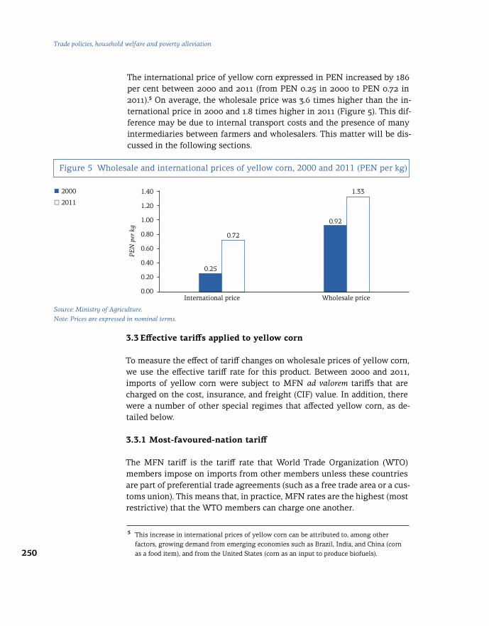
250
Trade policies, household welfare and poverty alleviation
The international price of yellow corn expressed in PEN increased by 186 per cent between 2000 and 2011 (from PEN 0.25 in 2000 to PEN 0.72 in 2011).5 On average, the wholesale price was 3.6 times higher than the in-ternational price in 2000 and 1.8 times higher in 2011 (Figure 5). This dif-ference may be due to internal transport costs and the presence of many intermediaries between farmers and wholesalers. This matter will be dis-cussed in the following sections.
Figure 5 Wholesale and international prices of yellow corn, 2000 and 2011 (PEN per kg)
Source: Ministry of Agriculture.Note: Prices are expressed in nominal terms.
3.3 Effective tariffs applied to yellow corn
To measure the effect of tariff changes on wholesale prices of yellow corn, we use the effective tariff rate for this product. Between 2000 and 2011, imports of yellow corn were subject to MFN ad valorem tariffs that are charged on the cost, insurance, and freight (CIF) value. In addition, there were a number of other special regimes that affected yellow corn, as de-tailed below.
3.3.1 Most-favoured-nation tariff
The MFN tariff is the tariff rate that World Trade Organization (WTO) members impose on imports from other members unless these countries are part of preferential trade agreements (such as a free trade area or a cus-toms union). This means that, in practice, MFN rates are the highest (most restrictive) that the WTO members can charge one another.
5 This increase in international prices of yellow corn can be attributed to, among other factors, growing demand from emerging economies such as Brazil, India, and China (corn as a food item), and from the United States (corn as an input to produce biofuels).
0.00
0.20
0.40
0.60
0.80
1.00
1.20
1.40
0.25
0.92
1.33
0.72
International price Wholesale price
PEN
per
kg
■ 2000
□ 2011

251
Peru
Estimation of the pass-through and welfare effects of the tariff reduction for yellow corn in Peru between 2000 and 2011
Between January 2000 and September 2007, the MFN tariff applied to Peruvian imports of yellow corn was 12 per cent. In the subsequent years, it was reduced to 9 per cent (October 2007), 6 per cent (January 2011), and zero (April 2011).
3.3.2 Additional tariff surcharge
In April 1997, the government added an ad valorem tariff of 5 per cent to the MFN tariff applied to yellow corn (Supreme Decree No. 035-97-EF). This policy was in force until June 2000.
3.3.3 Specific tariff
From August 1998 to May 2001, Peruvian importers of yellow corn had to pay a specific duty per metric ton that varied according to a free on board (FOB) reference price fixed by the central bank. The reference price changed every month and was an average of different market prices (USA 2YC-15.5 FOB Gulf and USA 3YC-15.5 FOB Pacific).6 When the FOB price reached a ceiling value (also established by the central bank), importers paid no additional duty. On the contrary, the duties increased when the FOB reference prices were reduced. In June 2001, this mechanism was re-placed by the Price Band System.
3.3.4 Price Band System
The Price Band System introduced in June 20017 increases or reduces the amount paid by importers resulting from the MFN tariff applied to yellow corn (and to other products such as milk, rice, and wheat). This amount is charged per metric ton – it can therefore be considered to be a specific tar-iff. It varies according to whether a CIF reference price is below (or above) a CIF floor price (or a CIF ceiling price):
• If the CIF reference price is below the floor, a specific duty per metric ton is added to the MFN ad valorem tariff.
• If the CIF reference price exceeds the ceiling, a specific duty per met-ric ton is detracted from the amount paid for the MFN ad valorem tariff. This reduction is applied up to a maximum of the MFN ad valorem tariff.
6 Supreme Decree No. 083-1998-EF. Available at: http://www.mef.gob.pe/index.php?option=com_ docman&task=cat_view&gid=127&limit=15&limitstart=60&order=date&dir= ASC&Itemid=100602&lang=es. 7 The Price Band System, introduced by Supreme Decree No. 115-2001-EF in June 2000, aimed to protect national agriculture from price distortions caused by agricultural policies of the major producers.

252
Trade policies, household welfare and poverty alleviation
The floor and ceiling prices, as well as the specific duties, are presented in a custom table established by the central bank. The table is published twice a year (1 January and 1 July) in the Official Gazette and includes a list of the CIF reference prices that will be in force during the coming semester. In addition, to establish which of the CIF prices listed in the custom table is applicable on a daily basis, the central bank fixes a reference CIF price every two weeks.
Table 1 summarizes the information from the custom table published on 1 July 2013. Using this information, we illustrate how to use the Price Band System. For instance, if a firm wants to import 10 metric tons of yellow corn on 5 August, it will have to search for the CIF reference price that is in force from 1 August to 15 August. In this case, the price is USD 239 per metric ton.8 According to Table 1, the latter price is below the floor price (USD 294), thus the importer has to pay a specific tariff of USD 56 per met-ric ton. Considering that since April 2011 the MFN ad valorem tariff has been zero, the total amount paid by the importer will be USD 560, which is equivalent to an ad valorem tariff of 23 per cent.9
8 To see this and other two-week reference CIF prices, go to: http://www.mef.gob.pe/index.php?option=com_docman&Itemid=100602. 9 Ratio of USD 560 to USD 2,390.
Table 1 Price Band System – Custom table, July–December 2013 (USD per metric ton)
CIF reference price USD 100-198
Additional or reduction specific tariff
CIF reference price USD 199-353
Additional or reduction specific tariff
CIF reference price USD 354-450
Additional or reduction specific tariff
100 200 199 98 354 -1
… … … … … …
138 160 237 58 392 -40
139 159 238 57 393 -41
140 158 239 56 394 -42
141 157 240 55 395 -44
142 156 241 54 396 -45
143 155 242 53 397 -46
144 154 243 52 398 -47
145 153 244 51 399 -48
… … … … … …
187 110 286 8 441 -91
188 109 287 7 442 -92
189 108 288 6 443 -93
190 107 289 5 444 -94
191 106 290 4 445 -95

253
Peru
Estimation of the pass-through and welfare effects of the tariff reduction for yellow corn in Peru between 2000 and 2011
10 If the volume imported from the United States does not exceed the quota established in the Agreement, importers do not have to pay duties. The Agreement established a duty-free tariff quota of initially 500,000 metric tons, with annual increases of 6 per cent and full duty-free access in 12 years. 11 The effective tariff rate plotted in Figure 6 is an indicative measure of the protection applied, but it does not represent the official formula used by Peruvian customs authorities. 12 The effective tariff cannot exceed the bound tariff to which Peru has committed under the WTO agreement (consolidated tariff), which is 68 per cent.
Source: Central Reserve Bank of Peru.
CIF reference price USD 100-198
Additional or reduction specific tariff
CIF reference price USD 199-353
Additional or reduction specific tariff
CIF reference price USD 354-450
Additional or reduction specific tariff
192 105 291 3 446 -96
193 104 292 2 447 -97
194 103 293 1 448 -98
195 102 294 0 449 -99
196 101 > 294 Floor Price 0 450 -100
197 100 < 353 Ceiling Price 0
198 99 353 0
3.3.5 Preferential tariffs
During the period covered by this study, Peru granted preferential tariffs to its main suppliers of yellow corn. In 2000, it offered a 100 per cent MFN reduction on its imports from Bolivia (under the Andean Agreement), and in 2006 it conceded a 15-year liberalization phase for Brazil and Argentina (under the Partial Preferential Agreement No. 58). In addition, in February 2009, the government granted the United States 100 per cent quota-free imports under the Trade Promotion Agreement.10
The effective tariff rate shown in Figure 611 is obtained as a ratio between the total amount of duties applied to imports of yellow corn and the total CIF imports of this crop:
Effective tariff ratet = ∑ Total duties on imports of yellow corn
∑ Total imports of yellow corn (1)
Figure 6 shows the monthly series (from January 2000 to December 2011) of the MFN ad valorem tariff rate and the effective tariff rate applied to Peruvian imports of yellow corn. There is an important difference between both series. Between January 2000 and November 2002, the effective tar-iff rate was higher than the MFN rate. In fact, during some months, the ef-fective tariff exceeded the MFN rate by more than 30 percentage points.12
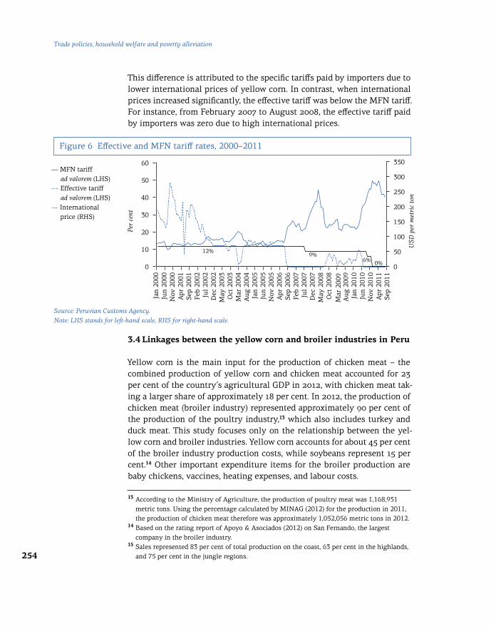
254
Trade policies, household welfare and poverty alleviation
This difference is attributed to the specific tariffs paid by importers due to lower international prices of yellow corn. In contrast, when international prices increased significantly, the effective tariff was below the MFN tariff. For instance, from February 2007 to August 2008, the effective tariff paid by importers was zero due to high international prices.
Figure 6 Effective and MFN tariff rates, 2000–2011
Source: Peruvian Customs Agency.Note: LHS stands for left-hand scale, RHS for right-hand scale.
3.4 Linkages between the yellow corn and broiler industries in Peru
Yellow corn is the main input for the production of chicken meat – the combined production of yellow corn and chicken meat accounted for 23 per cent of the country’s agricultural GDP in 2012, with chicken meat tak-ing a larger share of approximately 18 per cent. In 2012, the production of chicken meat (broiler industry) represented approximately 90 per cent of the production of the poultry industry,13 which also includes turkey and duck meat. This study focuses only on the relationship between the yel-low corn and broiler industries. Yellow corn accounts for about 45 per cent of the broiler industry production costs, while soybeans represent 15 per cent.14 Other important expenditure items for the broiler production are baby chickens, vaccines, heating expenses, and labour costs.
13 According to the Ministry of Agriculture, the production of poultry meat was 1,168,951 metric tons. Using the percentage calculated by MINAG (2012) for the production in 2011, the production of chicken meat therefore was approximately 1,052,056 metric tons in 2012. 14 Based on the rating report of Apoyo & Asociados (2012) on San Fernando, the largest company in the broiler industry. 15 Sales represented 83 per cent of total production on the coast, 63 per cent in the highlands, and 75 per cent in the jungle regions.
60
50
40
30
20
10 12%9%
6% 0%0
Per
cent
USD
per
met
ric
ton
350
300
250
200
150
100
50
0
Jan
2000
Jun
2000
Nov
200
0A
pr 2
001
Sep
2001
Feb
2002
Jul
2002
Dec
200
2M
ay 2
003
Oct
200
3M
ar 2
004
Aug
200
4Ja
n 20
05Ju
n 20
05N
ov 2
005
Apr
200
6Se
p 20
06Fe
b 20
07Ju
l 20
07D
ec 2
007
May
200
8O
ct 2
008
Mar
200
9A
ug 2
009
Jan
2010
Jun
2010
Nov
201
0A
pr 2
011
Sep
2011
― MFN tariff ad valorem (LHS)
– – Effective tariff ad valorem (LHS)
― International price (RHS)
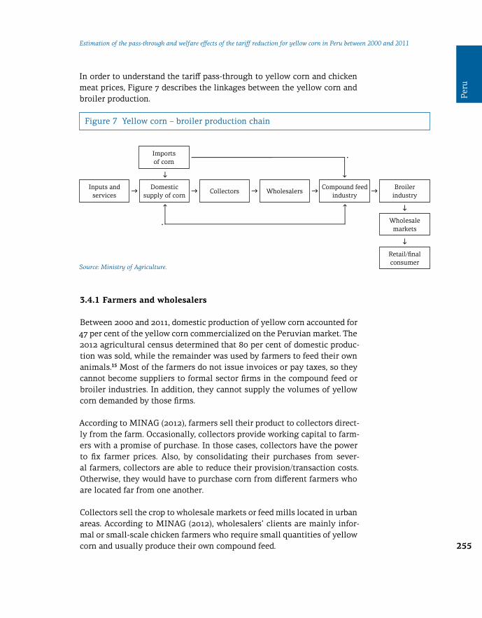
255
Peru
Estimation of the pass-through and welfare effects of the tariff reduction for yellow corn in Peru between 2000 and 2011
Figure 7 Yellow corn – broiler production chain
Source: Ministry of Agriculture.
3.4.1 Farmers and wholesalers
Between 2000 and 2011, domestic production of yellow corn accounted for 47 per cent of the yellow corn commercialized on the Peruvian market. The 2012 agricultural census determined that 80 per cent of domestic produc-tion was sold, while the remainder was used by farmers to feed their own animals.15 Most of the farmers do not issue invoices or pay taxes, so they cannot become suppliers to formal sector firms in the compound feed or broiler industries. In addition, they cannot supply the volumes of yellow corn demanded by those firms.
According to MINAG (2012), farmers sell their product to collectors direct-ly from the farm. Occasionally, collectors provide working capital to farm-ers with a promise of purchase. In those cases, collectors have the power to fix farmer prices. Also, by consolidating their purchases from sever-al farmers, collectors are able to reduce their provision/transaction costs. Otherwise, they would have to purchase corn from different farmers who are located far from one another.
Collectors sell the crop to wholesale markets or feed mills located in urban areas. According to MINAG (2012), wholesalers’ clients are mainly infor-mal or small-scale chicken farmers who require small quantities of yellow corn and usually produce their own compound feed.
Inputs and services
Domestic supply of corn
Importsof corn
CollectorsCompound feed
industryBroiler
industry
Wholesale markets
Retail/final consumer
Wholesalers→ →→ → →
↓
↓
↓
In order to understand the tariff pass-through to yellow corn and chicken meat prices, Figure 7 describes the linkages between the yellow corn and broiler production.
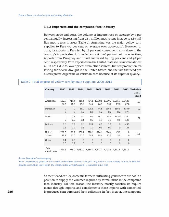
256
Trade policies, household welfare and poverty alleviation
3.4.2 Importers and the compound feed industry
Between 2000 and 2012, the volume of imports rose on average by 7 per cent annually, increasing from 0.85 million metric tons in 2000 to 1.83 mil-lion metric tons in 2012 (Table 2). Argentina was the major yellow corn supplier to Peru (70 per cent on average over 2000–2012). However, in 2012, its exports to Peru fell by 18 per cent; consequently, its share in the country’s imports shrank from 80 per cent to 68 per cent. At the same time, imports from Paraguay and Brazil increased by 103 per cent and 38 per cent, respectively. Corn exports from the United States to Peru were almost nil in 2012 due to lower prices from other sources, limited production fol-lowing the severe drought in the United States, and the fact that feed pro-ducers prefer Argentine or Peruvian corn because of its superior quality.
Table 2 Total imports of yellow corn by main suppliers, 2000–2012
Country 2000 2002 2004 2006 2008 2010 2011 2012 Variation 2011–2012
Argentina 562.966.5
719.478.6
815.375.0
954.164.2
1,070.676.9
1,059.755.7
1,515.179.8
1,242.367.8
–18
Paraguay 00
00
35.23.2
128.58.6
44.83.2
156.38.2
156.58.2
318.017.4
103
Brazil 00
0.10.0
0.60.1
0.70.0
54.03.9
58.93.1
163.08.6
225.712.3
38
Bolivia 0.60.1
1.50.2
5.60.5
25.11.7
8.20.6
2.30.1
00
45.32.5
United States
282.533.4
191.921.0
230.221.2
378.625.5
214.615.4
626.432.9
63.13.3
00
–100
Other 0.40.0
2.00.2
00
00
00
00
00
00
Total metric tons
846.4 915.0 1,087.0 1,486.9 1,392.2 1,903.5 1,897.8 1,831.3 –4
Source: Peruvian Customs Agency.Note: The imports of yellow corn are shown in thousands of metric tons (first line), and as a share of every country in Peruvian imports (second line, in per cent). The variation (the far right column) is expressed in per cent.
As mentioned earlier, domestic farmers cultivating yellow corn are not in a position to supply the volumes required by formal firms in the compound feed industry. For this reason, the industry mostly satisfies its require-ments through imports, and complements those imports with domestical-ly produced corn purchased from collectors. In fact, in 2011, the compound
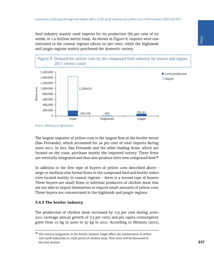
257
Peru
Estimation of the pass-through and welfare effects of the tariff reduction for yellow corn in Peru between 2000 and 2011
feed industry mainly used imports for its production (83 per cent of its needs, or 1.2 million metric tons). As shown in Figure 8, imports were con-centrated in the coastal regions (about 60 per cent), while the highlands and jungle regions mainly purchased the domestic variety.
Figure 8 Demand for yellow corn by the compound feed industry, by source and region, 2011 (metric tons)
Source: Ministry of Agriculture.
The largest importer of yellow corn is the largest firm in the broiler sector (San Fernando), which accounted for 26 per cent of total imports during 2000–2011. In fact, San Fernando and the other leading firms, which are located on the coast, purchase mainly the imported variety. These firms are vertically integrated and thus also produce their own compound feed.16
In addition to the first type of buyers of yellow corn described above – large or medium-size formal firms in the compound feed and broiler indus-tries located mainly in coastal regions – there is a second type of buyers. These buyers are small firms or informal producers of chicken meat that are not able to import themselves or require small amounts of yellow corn. These buyers are concentrated in the highlands and jungle regions.
3.4.3 The broiler industry
The production of chicken meat increased by 113 per cent during 2000–2011 (average annual growth of 7.3 per cent) and per capita consumption grew from 19 kg in 2000 to 37 kg in 2011. According to Shimizu (2011),
16 The vertical integration in the broiler industry might affect the transmission of yellow corn tariff reductions to retail prices of chicken meat. This issue will be discussed in the next section.
0
200,000
400,000
600,000
800,000
1,000,000
1,200,000
1,600,000
1,400,000
1,258,655
189,194 682 74,161
Coast Highlands Jungle
Met
ric
tons
■ Local production
□ Import

258
Trade policies, household welfare and poverty alleviation
increases in the production of chicken meat are due to the introduction of new technologies (i.e. breeding, nutrition, medicine, and equipment) and to the tendency towards vertical integration in the broiler industry.
The broiler industry is composed of about 30 large and medium-sized firms that account for 90 per cent of domestic production. The leading firms in 2012 were San Fernando (36 per cent of total sales), Redondos (19 per cent), Ganadera Santa Elena (12 per cent) and San Luis (4 per cent). Additionally, there are between 200 and 300 small firms, many of them subcontractors to the industry leaders. The main producing areas are located in the coast-al regions: in 2012, Lima accounted for 55 per cent of domestic production, followed by La Libertad (20 per cent), Arequipa (9 per cent), and Ica (4 per cent).17 The firms are close to the coast because most of the facilities of the broiler industry (such as breeding farms, hatchery plants, feed mills, grow-out farms, slaughtering plants, and processing plants) are located there. Moreover, they are close to the Ports of Callao (Lima), Pisco (Ica), and Salaverry (La Libertad), the main points of entry for imported corn.
The most important characteristic of the Peruvian broiler industry is re-lated to its distribution process. In developed countries, almost all broilers are slaughtered and processed before they are distributed to wholesalers. In Peru, by contrast, around 80 per cent of broilers are distributed alive to wholesalers (Shimizu, 2011), and according to MINAG (2012) approximate-ly 65 per cent are sold in Lima.
4 Methodology and results
4.1 Tariff and price pass-through estimation
The previous section identified two patterns of yellow corn demand: the coast meets its demand mainly through imports, while the highlands and jungle regions consume mostly domestically produced corn. Therefore, one would expect that trade policy measures that reduce tariffs on yellow corn would have a more significant effect on the coast.
In this context, the objective of this study is to estimate the extent of the tariff pass-through to domestic prices in the coastal regions of Peru due to the reduction in yellow corn tariffs between 2000 and 2011. Given the im-portance of yellow corn as an input for the production of chicken meat and, in turn, the importance of chicken meat in the Peruvian food expenditure
17 Data from the Ministry of Agriculture.

259
Peru
Estimation of the pass-through and welfare effects of the tariff reduction for yellow corn in Peru between 2000 and 2011
basket, we also measure the extent to which tariff reductions on yellow corn have translated into changes in household welfare in the coastal re-gions through the consumption of chicken meat.18
This section first estimates the tariff pass-through to wholesale prices of yellow corn and then examines the price pass-through of yellow corn to retail prices of chicken meat.
Following the theoretical framework applied in Nicita (2009), we start with the estimation of the tariff pass-through coefficient in the yellow corn market, for which it is assumed there are no differences between imported and domestic varieties of yellow corn. However, given that yellow corn is not consumed directly by households, but used as a production input for the chicken meat (broiler) industry, we will use wholesale prices of yellow corn instead of retail prices as our dependent variable. We will model yel-low corn wholesale prices (pdit ) as a function of yellow corn producer pric-es (ppit ), yellow corn international prices in domestic currency (p *t ) , trade costs (trct ),
19 an index of market concentration (mrkct ), effective tariffs (ett), and a trend variable (year).20 This can be expressed in logarithms as:
ln pdit = β1 + β2 ln ppit + β3 ln p *t + β4 ln trct + β5 ln mrkct + γ ln (1 + ett ) (2) + θ yeart + εit
where i is the subscript associated with regions and t is the subscript as-sociated with monthly periods.
The tariff pass-through elasticity is represented by γ, the percentage in-crease in local prices derived from a 1 per cent increase in the tariff. In or-der to estimate the tariff pass-through for yellow corn, we will use monthly data21 from January 2000 to April 2011 for eight coastal regions of Peru where most of the production of and demand for yellow corn are concen-trated.22 Our panel database is balanced. Wholesale and producer (farm)
18 Originally we also intended to measure the impact on producer welfare on the coast. However, there were no households/units of production of corn/chicken meat represented in the 2011 Household Survey for the coastal regions that reported income resulting from the sale of these items. Therefore, we only focused on the analysis of the impact on consumer welfare. 19 Trade costs are assumed to affect only imported goods. 20 To capture the effect of a trending factor common to all coastal regions (such as the influence of demand preferences and agricultural policies). 21 A description of our statistical sources is presented in the Annex. 22 Lambayeque, La Libertad, Ancash, Lima, Ica, Arequipa, Moquegua, and Tacna. Two regions on the coast (Tumbes, Piura) were excluded due to the fact that they registered few observations of the dependent variable.

260
Trade policies, household welfare and poverty alleviation
prices of yellow corn are available by region. The international price of yellow corn corresponds to the closing spot price of yellow corn number 2 on the Chicago Commodities Exchange, expressed in local currency (PEN). The effective tariff includes the MFN tariff and specific/additional tariffs that were in force during the period covered by this analysis. Trade costs are measured as monthly averages of freight and insurance costs per unit (kg) of Peruvian imports of yellow corn. The index of market concentration is the C4 market share23 of yellow corn importing firms in Peru.
We estimate two panel data specifications to explain the behaviour of the dependent variable (wholesale yellow corn prices) using fixed- and ran-dom-effects estimation.24 Due to the fact that we are working with differ-ent regions on the coast of Peru, it seems reasonable to assume that there is a component of time-invariant unobserved heterogeneity across entities, which could be correlated with some explanatory variables (e.g. differenc-es in productivity and entrepreneurial behaviour may be correlated with producer prices). Therefore, to allow for arbitrary correlation between re-gional unobserved heterogeneity and the predictor variables, we estimate a fixed-effects model, whose results will then be compared with those of a random-effects model through a Hausman test.
Given that a reverse causality relationship exists between yellow corn pro-ducer prices and wholesale prices (endogeneity), contemporary produc-er prices in both models are instrumented by their four-month lag, using two-stage least squares.
In both models, all coefficients are significant at the 1 per cent confidence level and with the expected signs (all positive). According to the results of the Hausman test, the null hypothesis of no systematic differences between fixed- and random-effects estimators cannot be rejected, so we should take the coefficients from the random-effects model25 to estimate the welfare effects on households on the coast of Peru derived from the tariff changes in yellow corn (and the changes in chicken meat prices that those changes induce).
As shown in Table 3, our tariff pass-through coefficient for wholesale pric-es of yellow corn is 0.74, which suggests a moderate to high transmission
23 The aggregated market share of the four biggest importers. 24 We do not estimate our panel by ordinary least squares because the necessary assumption of zero correlation between the error term and the explanatory variables would be violated. 25 In this context, this model provides consistent, more efficient results than fixed-effects estimation.
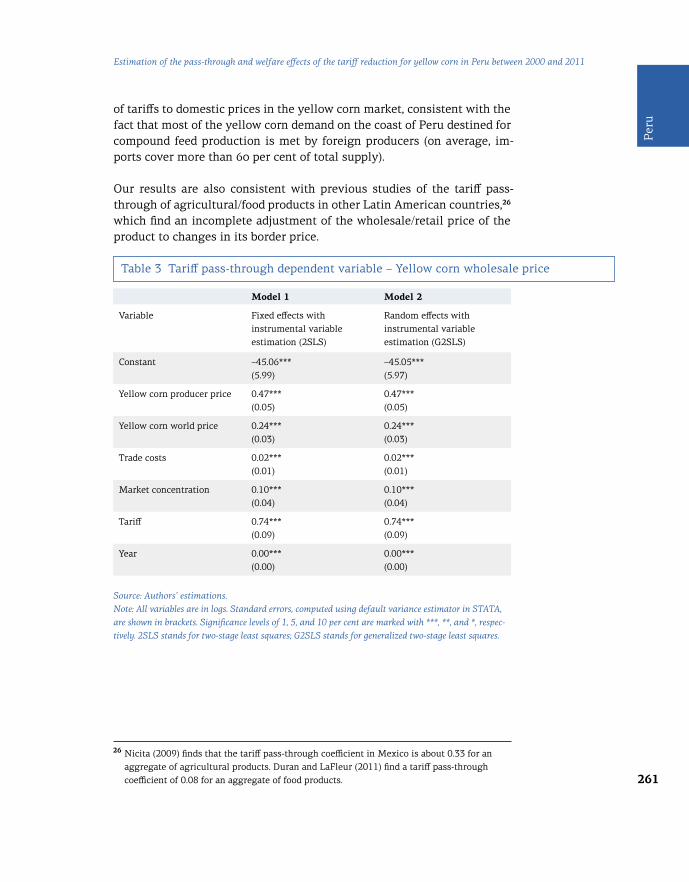
261
Peru
Estimation of the pass-through and welfare effects of the tariff reduction for yellow corn in Peru between 2000 and 2011
26 Nicita (2009) finds that the tariff pass-through coefficient in Mexico is about 0.33 for an aggregate of agricultural products. Duran and LaFleur (2011) find a tariff pass-through coefficient of 0.08 for an aggregate of food products.
Model 1 Model 2
Variable Fixed effects with instrumental variable estimation (2SLS)
Random effects with instrumental variable estimation (G2SLS)
Constant –45.06*** (5.99)
–45.05***(5.97)
Yellow corn producer price 0.47***(0.05)
0.47***(0.05)
Yellow corn world price 0.24***(0.03)
0.24***(0.03)
Trade costs 0.02***(0.01)
0.02***(0.01)
Market concentration 0.10***(0.04)
0.10***(0.04)
Tariff 0.74***(0.09)
0.74***(0.09)
Year 0.00***(0.00)
0.00***(0.00)
Source: Authors’ estimations.Note: All variables are in logs. Standard errors, computed using default variance estimator in STATA, are shown in brackets. Significance levels of 1, 5, and 10 per cent are marked with ***, **, and *, respec-tively. 2SLS stands for two-stage least squares; G2SLS stands for generalized two-stage least squares.
of tariffs to domestic prices in the yellow corn market, consistent with the fact that most of the yellow corn demand on the coast of Peru destined for compound feed production is met by foreign producers (on average, im-ports cover more than 60 per cent of total supply).
Our results are also consistent with previous studies of the tariff pass-through of agricultural/food products in other Latin American countries,26 which find an incomplete adjustment of the wholesale/retail price of the product to changes in its border price.
Table 3 Tariff pass-through dependent variable – Yellow corn wholesale price

262
Trade policies, household welfare and poverty alleviation
Had the movement in the wholesale price of yellow corn been determined exclusively by the effective tariff cut, the wholesale price would have ex-perienced a reduction of 24.68 per cent (Table 5), which is obtained as the result of multiplying the tariff reduction (–33.3 per cent) by the tariff pass-through coefficient (0.74) estimated over the period 2000–2011.
We next address the pass-through between wholesale prices of yellow corn (as a production input) and retail prices of chicken meat, given that we want to measure the welfare effects on coastal households derived from the consumption of chicken meat, which is an important item in the food expenditure basket.
For this estimation, we also use monthly data27 from January 2000 to April 2011 from the most representative coastal region (Lima).28 Here we use the retail price of chicken meat as the dependent variable, and include as ex-planatory variables the wholesale price of yellow corn and the internation-al price of soybeans (both production inputs for the compound feed used by the broiler industry),29 as well as the retail price of fish meat (to allow for the possibility of substitution between chicken and fish in household demand).30
As shown in Table 4, we obtained a price pass-through coefficient from yel-low corn to chicken meat of 0.22, which is significant at the 1 per cent con-fidence level and has the expected sign. Despite the fact that yellow corn accounts for more than 60 per cent of compound feed production costs on the coast, the magnitude of the price pass-through coefficient is consistent with the fact that there is evidence of a relatively high concentration in the broiler industry (in 2012, the market share of the four biggest firms in Lima was 70 per cent). Moreover, there is vertical integration in the firms that are both the biggest importers of yellow corn and the major produc-ers of chicken meat, which suggests that limitations in competition may have hindered the transmission of the tariff reduction to the prices of yel-low corn and chicken meat for consumers on the coast.
27 A description of our statistical sources is presented in the Annex. 28 According to MINAG (2012), 65 per cent of chicken meat sales take place in Lima. 29 Compound feed costs account for approximately 75 per cent of production costs in the broiler industry. 30 We also included the retail prices of red meat and pork, gasoline prices, and an index of wholesale price inflation in the estimation, but they were rendered insignificant.

263
Peru
Estimation of the pass-through and welfare effects of the tariff reduction for yellow corn in Peru between 2000 and 2011
31 Obtained by subtracting the average effective tariff in 2011 from the average effective tariff in 2000.
Model 1
Variable Ordinary least squares
Constant 1.49***(0.07)
Yellow corn wholesale price0.22***(0.07)
Soybean world price0.10***(0.04)
Fish retail price0.20***(0.04)
Product Yellow corn tariff change (per cent)
Tariff pass-through rate (fraction)
Price pass-through rate from yellow corn to chicken meat (fraction)
Price change attributed to yellow corn tariff change (per cent)
Yellow corn −33.28 0.74 −24.68
Chicken meat −33.28 0.74 0.22 −5.50
Source: Authors’ estimations.Note: All variables are in logs. Standard errors, computed using default variance estimator in STATA, are shown in brackets. Significance levels of 1, 5, and 10 per cent are marked with ***, **, and *, respectively.
Source: Authors’ estimations. Note: The changes were estimated for the 2000–2011 period. The tariff pass-through rate was taken from the estimation results for the tariff variable in Table 3 (Model 1). The price pass-through rate from yellow corn to chicken meat was taken from the estimation results for the yellow corn wholesale price variable in Table 4. The price changes in the last column are the result of multiplying the factors in each row.
Table 4 Price pass-through dependent variable – Chicken meat retail price
Table 5 Chicken meat price changes induced by yellow corn tariff changes
For the estimation of household welfare changes, we use a retail price change for chicken meat induced by the tariff reduction in yellow corn equal to –5.5 per cent. It is obtained by multiplying the tariff change31 be-tween 2000 and 2011 (−33.28 per cent, as shown in Figure 9) by both the tariff pass-through rate (0.74) and the price pass-through rate from yellow corn to chicken meat (0.22).

264
Trade policies, household welfare and poverty alleviation
Figure 9 Effective tariff for yellow corn, annual average, 2000–2011 (per cent)
Source: Peruvian Customs Authority.
As mentioned previously, despite the reduction in the tariff applied to yel-low corn during 2000–2011, wholesale yellow corn prices rose by 31.1 per cent and retail prices of chicken meat rose by 28.4 per cent during the same period. Nevertheless, our estimation results suggest a reduction of 24.68 per cent in yellow corn prices and 5.5 per cent in chicken meat pric-es induced by the yellow corn tariff reduction (see Table 5). A counterfac-tual interpretation of these results implies that, if the tariffs had not been reduced, local prices of yellow corn and chicken meat would have risen by 55.78 per cent and 33.9 per cent, respectively. This shows that the meas-ures adopted mitigated increases in local prices that would otherwise have been observed.
4.2 Estimation of welfare changes
This section measures the extent to which tariff reductions in yellow corn have affected household welfare through consumption of chicken meat, considering only first-order consumption effects.
First, using non-parametric regression methods, we analyse the relation-ship between per capita expenditure of the households located on the coast of Peru and the welfare effects derived from the changes in retail prices of chicken meat induced by the tariff reduction in yellow corn. This analysis is conducted according to two criteria: (a) rural/urban location, and (b) pov-erty characteristics in terms of monetary poverty (i.e. non-poor, poor, and extremely poor households).
20000.0
5.0
10.0
15.0
20.0
25.0
30.0
35.0
29.5
19.4
11.69.8
12.9
9.1
0.0 0.00.8
3.6 3.9
33.3
2002 2004 2006 2008 20102001 2003 2005 2007 2009 2011
Per
cent

265
Peru
Estimation of the pass-through and welfare effects of the tariff reduction for yellow corn in Peru between 2000 and 2011
Figure 10 Kernel density estimation of per capita expenditure
Source: Authors’ estimations, based on the 2011 National Household Survey.
We work with data from the 2011 National Household Survey in Peru, which included 9,561 households on the coast. Eighty-six per cent (8,262) of surveyed households on the coast were in urban areas. The number of households that recorded a non-zero consumption share of chicken meat was 7,270.32 Even though the majority of chicken meat production units are located on the coast of Peru, these firms are not represented in the household survey, which implies that we are only able to measure the wel-fare changes on the consumption side.
Following Deaton (1989), we use a kernel density estimator to character-ize a smooth density function of log of per capita expenditure.33 As shown in Figure 10, urban areas present higher levels of expenditure than rural areas.
32 According to the survey, 2,291 households recorded a zero consumption share of chicken meat. 33 We use Epanechnikov kernel and bandwidth = 0.5. 34 Inferior goods refer to such products as potatoes, rice, entrails and offal, among others.
As shown in Table 6, chicken meat accounts on average for 4.28 per cent of household expenditure on the coast. On average, consumption shares of chicken meat are higher in urban than in rural areas on the coast, with the highest share in the capital (Metropolitan Lima). In addition, poor house-holds show a higher consumption share of chicken meat than non-poor households, while extremely poor households have the lowest expendi-ture share, as it is likely that inferior goods have the highest shares in their food consumption basket.34
.5
.3
.4
.2
.1
0
7 8 9 10
Den
sity
Log per capita expenditure
― Coast
– – Urban coast
Rural coast
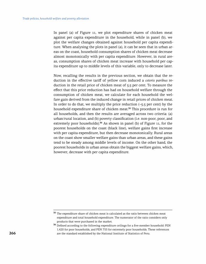
266
Trade policies, household welfare and poverty alleviation
In panel (a) of Figure 11, we plot expenditure shares of chicken meat against per capita expenditure in the household, while in panel (b), we plot the welfare changes obtained against household per capita expendi-ture. When analysing the plots in panel (a), it can be seen that in urban ar-eas on the coast, household consumption shares of chicken meat decrease almost monotonically with per capita expenditure. However, in rural are-as, consumption shares of chicken meat increase with household per cap-ita expenditure up to middle levels of this variable, only to decrease later.
Now, recalling the results in the previous section, we obtain that the re-duction in the effective tariff of yellow corn induced a ceteris paribus re-duction in the retail price of chicken meat of 5.5 per cent. To measure the effect that this price reduction has had on household welfare through the consumption of chicken meat, we calculate for each household the wel-fare gain derived from the induced change in retail prices of chicken meat. In order to do that, we multiply the price reduction (–5.5 per cent) by the household expenditure share of chicken meat.35 This procedure is run for all households, and then the results are averaged across two criteria: (a) urban/rural location, and (b) poverty classification (i.e. non-poor, poor, and extremely poor households).36 As shown in panel (b) of Figure 11, for the poorest households on the coast (black line), welfare gains first increase with per capita expenditure, but then decrease monotonically. Rural areas on the coast show smaller welfare gains than urban areas, and these gains tend to be steady among middle levels of income. On the other hand, the poorest households in urban areas obtain the biggest welfare gains, which, however, decrease with per capita expenditure.
35 The expenditure share of chicken meat is calculated as the ratio between chicken meat expenditure and total household expenditure. The numerator of the ratio considers only products that were purchased in the market. 36 Defined according to the following expenditure ceilings for a five-member household: PEN 1,420 for poor households, and PEN 755 for extremely poor households. These references are the standard established by the National Institute of Statistics of Peru.

267
Peru
Estimation of the pass-through and welfare effects of the tariff reduction for yellow corn in Peru between 2000 and 2011
Figure 11 Expenditure shares and welfare changes due to the impact of yellow corn tariff reductions on consumption of chicken meat
Source: Authors’ estimations, based on the 2011 National Household Survey.
The results in Table 6 show that the reduction in chicken meat retail prices induced by the tariff reduction for yellow corn generates an average wel-fare gain of 0.24 per cent. Due to the fact that urban areas show a high-er consumption share of chicken meat than rural areas, welfare gains are slightly higher in the former (0.24 per cent versus 0.22 per cent). Also, it can be seen that the induced effects of yellow corn tariff reductions have a pro-poor bias. Poor households on the coast get the highest welfare gain of 0.29 per cent, compared to the non-poor group (0.23 per cent).
(a)
(b)
6
.3
4
5
.25
3
.2
2
.15
7
7
8
8
9
9
10
10
Log per capita expenditure per household
Log per capita expenditure per household
Wel
fare
gai
nEx
pend
itur
e sh
are
― Coast
― Urban coast
Rural coast
― Coast
― Urban coast
Rural coast

268
Trade policies, household welfare and poverty alleviation
Coastal areas Average expenditure share of chicken meat
Average welfare gain
Center 4.38 0.24
North 4.19 0.23
South 3.75 0.21
Metropolitan Lima 4.59 0.25
Urban 4.32 0.24
Rural 4.02 0.22
Non-poor 4.15 0.23
Extremely poor 3.48 0.19
Poor 5.19 0.29
Total coast 4.28 0.24
Table 6 Average welfare changes due to the impact of yellow corn tariff reductions on consumption of chicken meat (per cent)
Source: Authors’ estimations.
5 Conclusions and policy recommendations
In recent years, the effectiveness of tariff reductions applied to yellow corn imports in Peru has come under scrutiny because their expected benefits do not seem to have been significantly transferred to buyers of yellow corn and of its main derivative product, chicken meat. While the effective tariff of yellow corn was reduced by 33.3 percentage points between 2000 and 2011, average prices of yellow corn and chicken meat increased by 31.1 per cent and 28.4 per cent, respectively.
This study used two approaches to try to provide a tentative explana-tion to this apparent mismatch between the reduction of tariffs and the increase of domestic prices by undertaking: (a) estimations of the tariff pass-through to domestic prices of yellow corn and chicken meat; and (b) estimations of the first-order household welfare effects – excluding effects on wages – induced by the tariff reduction for yellow corn.
First, the estimation results show that the tariff reduction for yellow corn helped mitigate increases in local prices of yellow corn and chicken meat that otherwise would have occurred. In fact, a counterfactual interpreta-tion of these results implies that if the tariffs had not been reduced, local prices of yellow corn and chicken meat would have risen by 55.78 per cent and 33.90 per cent, respectively.
Second, the findings show that the reduction in chicken meat retail pric-es induced by the tariff reduction for yellow corn would have generated an

269
Peru
Estimation of the pass-through and welfare effects of the tariff reduction for yellow corn in Peru between 2000 and 2011
average welfare gain of 0.24 per cent on the coast of Peru. Slightly higher welfare gains would have been obtained in urban areas (0.24 per cent) as opposed to rural areas (0.22 per cent). The estimated effect of yellow corn tariff reductions would have had a pro-poor bias, with poor households ob-taining the highest welfare gain (0.29 per cent), compared to the non-poor group (0.23 per cent).
However, the results suggest that the benefits of the tariff reduction may not have been fully transmitted to consumers, and it could be the case that they have mostly been captured by the firms importing yellow corn and by the largest broiler producers, which are vertically integrated firms.
As regards the effects on producer welfare, we were not able to capture them because no income resulting from the sales of yellow corn and chicken meat was reported in the household survey for coastal regions. However, as the theory suggests, we would expect that net producers of yellow corn and derived products would have incurred welfare losses as a result of the tariff reduction.
In line with previous findings in the applied literature on trade policy transmission to household welfare, this study showed that when design-ing tariff policies that should mostly benefit consumers, special attention needs to be paid to the design of complementary policies aimed at encour-aging a greater degree of competition in the relevant market. In this case, while there is some evidence that the yellow corn market in Peru is mod-erately competitive, the opposite happens to be true in the broiler indus-try, where the four biggest producers account for 70 per cent of total sales in Lima, and the major players are vertically integrated.
In addition, different patterns of yellow corn demand by the broiler indus-try on the coast (met mainly through imports) versus the highlands and jungle regions (which mostly use locally produced corn) suggest a low de-gree of integration in the national yellow corn market. This is also reflect-ed in the significant differences in wholesale prices of yellow corn across regions. Therefore, trade policy measures aimed at altering tariffs for yel-low corn would have had a more significant effect on the coast and a mar-ginal effect on the highlands and jungle regions. This result highlights the importance of furthering market integration as a means of extending the benefits of trade policy, particularly to the poorest groups in the high-lands and jungle regions. In sum, the effectiveness of tariff reductions such as those in the Peruvian yellow corn market should be increased through port and highway infrastructure development in order to enhance market integration.

270
Trade policies, household welfare and poverty alleviation
Variable Primary sources
Yellow corn wholesale pricesMinistry of Agriculture, National Institute of Statistics
Yellow corn producer pricesMinistry of Agriculture, National Institute of Statistics
Yellow corn world prices (yellow corn no. 2 – Chicago Commodities Exchange)
Reuters/Bloomberg
Trade costs (average freight and insurance costs per kg of Peruvian imports of yellow corn)
Peruvian Customs Agency – calculated by the authors
Market concentration (C4 market shares of yellow corn importing firms in Peru)
Peruvian Customs Agency – calculated by the authors
Effective tariffs on yellow corn Peruvian Customs Agency
Chicken meat retail prices National Institute of Statistics
Soybean world prices Reuters/Bloomberg
Fish meat retail prices National Institute of Statistics
Nominal exchange rates (USD/PEN) Central Reserve Bank of Peru
Table A1 Data sources
Source: Authors’ estimations.
Annex

271
Peru
Estimation of the pass-through and welfare effects of the tariff reduction for yellow corn in Peru between 2000 and 2011
References
Apoyo & Asociados (2012). Rating report on San Fernando S.A. June.
Deaton, A. (1989). “Rice Prices and Income Distribution in Thailand: A Non-Parametric Analysis.” Economic Journal, 99 (395): 1–37.
Duran, J. and LaFleur, M. (2011). “Effects of Trade Opening on Household Welfare: The Chilean Case.” Serie Comercio Internacional No. 114. United Nations Economic Commission for Latin America and the Caribbean, Santiago de Chile.
MINAG (2012). “Maíz Amarillo Duro. Principales Aspectos de la Cadena Agroproductiva.” Ministry of Agriculture of Peru [online]. Available at: http://agroaldia.minag.gob.pe/biblioteca/download/pdf/agroeconomia/agroeconomiamaizamarillo2.pdf.
Nicita, A. (2009). “The Price Effect of Tariff Liberalization: Measuring the Impact on Household Welfare.” Journal of Development Economics, 89 (1): 19–27.
Shimizu, T. (2011). “Development of Broiler Integration in Peru.” IDE Discussion Paper No. 298. Institute of Developing Economies, Chibe.

272
Trade policies, household welfare and poverty alleviation
Nigeria

273
Nig
eria
The welfare impact in Nigeria of the ECOWAS Common External Tariff: A distributional effects analysis
Abstract
Trade policies often have a different impact on economic agents due to the transmission mechanism through which they operate. In this context, this study uses micro- and macro-economic data to investigate the distribu-tional effects in Nigeria of the Common External Tariff of the Economic Community of West African States. These effects are examined from the perspective of households as producers, consumers, and factor owners. The analysis proceeds in three steps investigating: (a) the tariff pass-through to domestic prices, (b) the linkages between prices and wages, and (c) the im-pact of both prices and wages on household welfare. The findings indicate that during the period covered by this study, domestic prices declined due to the high tariff pass-through. This decline was higher in the states located closer to ports and borders, where the costs of trade are lower. The Common External Tariff had net positive effects on the welfare of households, largely due to the gains from the expenditure basket. The expenditure gains through lower prices outweighed losses in households’ purchasing power incurred through lower income. Poorer households experienced larger welfare gains than richer ones, and urban households were better off than their rural coun-terparts. The study concludes that the price transmission mechanism and household characteristics are important determinants in assessing trade policy effects in Nigeria. Concerning the price-wage nexus, it does not find strong evidence of price influence on wages. The study suggests that com-petitiveness of domestic producers should be enhanced through investment in infrastructure and strengthening of relevant government programmes to create employment and improve household income in agriculture and the manufacturing sector. It also recommends social safety net measures, par-ticularly for vulnerable subsistence agricultural households in rural areas, in order to mitigate the effects of the Common External Tariff on their income.
* The author would like to thank Suleman Adebayo Audu, Minister from the Permanent Mission of Nigeria to the United Nations at Geneva, Nigeria Trade Office to the World Trade Organization (WTO), for his support in the preparation of this study, Dare Alaba for her research assistance, Idri Ademuyiwa for helping to obtain data from the National Bureau of Statistics, Fatima O. Kareem for assisting with the analysis, and Marco Sanfilippo, Kristina Czura, Timea Pal, Johanna Gereke and Andrej Tusicisny from the Development Study Working Group, European University Institute, Italy, for their comments on the study.
Olayinka Idowu Kareem *

274
Trade policies, household welfare and poverty alleviation
1 Introduction
The economic integration of developing countries such as Nigeria into global markets offers the opportunity for rapid growth and poverty re-duction (Martinez and Poole, 2004), but it also entails risks. For example, Nigeria is endowed with abundant natural resources, especially crude oil, from which it derives over 90 per cent of its foreign earnings. The country has experienced average growth of around 7 per cent during the past five years. However, this growth has not trickled down to the major-ity of the population, thus reinforcing Nigeria’s status as a rich country populated by poor people (World Bank, 1996). The unemployment rate reached 24 per cent in 2011 (NBS, 2012a) and the share of the popula-tion living below the poverty line increased from 54 per cent in 1986 to 68 per cent in 2010.1
Explaining Nigeria’s situation demands a careful analysis of government policies and their effects. This study will focus in particular on the trade dimension and analyse the impact on household welfare of Nigeria’s adop-tion of the Common External Tariff (CET) of the Economic Community of West African States (ECOWAS).2
To integrate its economy into global markets, particularly in the ECOWAS sub-region, Nigeria committed itself in 2005 to adopting the ECOWAS CET. During the transition period of 2006–2007, it therefore reduced its tariff rates on all products from a high of 150 per cent to a maximum of 50 per cent.3
The CET represents the most-favoured-nation (MFN) rates ECOWAS applies in relation to non-member countries and is part of the move towards a customs union that aims to enhance sub-regional trade inte-gration through the flow of goods and services, especially inputs and in-termediate goods for the industrial sector. The ECOWAS CET has four tariff bands: 0 per cent for social needs and basic necessities, 5 per cent for raw materials, 10 per cent for intermediate goods, and 20 per cent for
1 Data from the World Bank World Development Indicators database, available at: http://data.worldbank.org/data-catalog/world-development-indicators. 2 The 15 West African states that constitute ECOWAS are: Benin, Burkina Faso, Cape Verde, Côte d’Ivoire, the Gambia, Ghana, Guinea, Guinea-Bissau, Liberia, Mali, Niger, Nigeria, Senegal, Sierra Leone and Togo. 3 This was the maximum tariff rate on both goods and services during the country’s transition period leading to the adoption of the CET. 4 The four bands mentioned above are the current ECOWAS CET bands and are not the same as the bands Nigeria used during the transition period.

275
Nig
eria
The welfare impact in Nigeria of the ECOWAS Common External Tariff: A distributional effects analysis
finished goods that are not produced locally. Nigeria was granted the pos-sibility of adding a fifth band of 35 per cent for finished goods manufac-tured locally.4 Following the adoption of the CET, Nigeria’s simple average tariff on agricultural imports dropped from about 32 per cent in 2000 to 15 per cent in 2010, while its tariff on manufactured products fell from 25 per cent in 2000 to 11 per cent in 2010.5
Nigeria accounts for more than half of the sub-region’s imports. In nom-inal terms, its total imports increased from USD 6 billion in 1990 to USD 64 billion in 2011, while ECOWAS’s total imports rose from USD 14 bil-lion in 1990 to USD 111 billion in 2011 (UNCTAD, 2012). In terms of import composition, Nigeria accounted for 40 per cent of ECOWAS’s agricultur-al imports in 2009 and 79 per cent in 2011, while its industrial imports represented 79 per cent and 65 per cent of those of ECOWAS in 2009 and 2011, respectively. These data confirm the huge trade impact of Nigeria on the sub-region and explain its late and reluctant acceptance of the ECOWAS CET.
In addition, Nigeria’s imports from ECOWAS declined over the years in terms of their share in the country’s total imports. In 1994, the share of imports from ECOWAS in Nigeria’s total imports was about 5 per cent. It then declined to 3.2 per cent in 2005, and fell further to 2.3 per cent in 2012 (IMF, 2013).6 This reduction in the flow of imports from ECOWAS to Nigeria was a result of inadequate infrastructure and implementation of the sub-regional trade liberalization scheme.7
The adoption of the CET has had different effects on Nigerian households, depending on whether they are net consumers or producers of commodi-ties, and on household labour returns. The literature on the transmission mechanism and welfare impact of this type of trade policy does not provide unequivocal conclusions. The different transmission channels through which trade policies operate are usually responsible for the variation of
5 Data from the World Bank World Integrated Trade Solution (WITS) database, available at: http://wits.worldbank.org/wits. 6 This suggests that more than 97 per cent of Nigeria’s imports of goods and services in 2012 came from countries outside ECOWAS. UNCTAD (2012) shows that less than 7 per cent of Nigeria’s imports are sourced from Africa. 7 The sub-regional trade liberalization scheme, which covers unprocessed goods, traditional handicrafts, and processed and semi-processed goods originating from member countries, aims to ensure the free flow of goods and services across members without subjecting them to tariffs and non-tariff barriers. However, in reality this is not the case, due to bureaucratic processes, lengthy import procedures, corruption in customs and road transport, etc. For more details, see Section 2.

276
Trade policies, household welfare and poverty alleviation
the effects.8 Most often, trade policies affect domestic prices and returns to production factors (labour), which in turn have effects on the consumption and production decisions of households (Nicita, 2004, 2009; Goldberg and Pavcnik, 2003, 2007; Marchand, 2012; Topalova, 2005, 2010; Porto, 2006; McCaig, 2011; Castilho et al., 2012). This study therefore asks the following questions: To what extent has the ECOWAS CET affected domestic prices? And what has been its effect on household welfare?
In order to address these questions, this study conducts an empirical inves-tigation of the distributional effects of the ECOWAS CET in Nigeria. These effects consist mainly of the impact on the markets where the households operate, on the goods they produce, and on the labour markets where they are active. It is therefore important for the Nigerian government to be aware of the level of CET pass-through to domestic prices, and to ascertain the effects of the price changes on factor income and household welfare. Providing this critical information is the primary objective of this study.
Despite the wide range of analysis in the literature on the distributional im-pact of trade liberalization, very few studies evaluate the trade liberalization policy of the ECOWAS CET in Nigeria. Balogun and Dauda (2012), Urama et al. (2012), Oduh (2012), Ajayi and Osafo-Kwaako (2007), Oyejide (2012), and Nwafor (2006) look only at the macroeconomic impact of the CET on Nigeria. The potential distributional impact has been examined exclusively through ex-ante studies: Nwafor et al. (2005) use a Computable General Equilibrium (CGE) model to examine the potential impact of the adoption of the CET on rural and urban poverty, and Marchat and Rajhi (2004), Soludo and Oji (2003), and Kuji Ltd. (2002) conduct ex-ante analyses at the sectoral and household levels. There are few, if any, ex-post studies that examine the distribution-al effects of the ECOWAS CET on Nigerian households or the level of tar-iff pass-through onto the country’s domestic prices. This study aims to fill this gap by analysing the impact of the ECOWAS CET on Nigeria’s house-holds through an ex-post econometric analysis using household survey data.
The empirical strategy of this study was adopted from Nicita (2009), Porto (2006), and Marchand (2012). The price effects on household welfare
8 While this study focuses on the price and factor return effects of the ECOWAS CET, it is acknowledged that there are other effects that should also be considered, such as those related to employment, agricultural outputs, and investment. 9 Due to inconsistencies in the implementation of the scheme by members, there are still non-tariff barriers such as certificates of origin, standards requirements, bureaucratic problems, unofficial fees, delays at borders, waste and theft at ports, harassment by the police and other security agents at a number of locations, and inter-country payment difficulties (ECOWAS Vanguard, 2013).

277
Nig
eria
The welfare impact in Nigeria of the ECOWAS Common External Tariff: A distributional effects analysis
depend on the budget share of each commodity, the share of household in-come from the commodity, and the price change of the commodity due to trade. The methodology first determines the impact of the ECOWAS CET on domestic prices; it then examines the linkage between domestic pric-es and wages. The final analysis combines the effects of price and wage changes on household welfare. The results show that the ECOWAS CET has net positive effects on household welfare, mainly due to the gains from the expenditure basket. During the period covered by the study, consumers benefited from the CET through the expenditure gains that outweighed the losses due to lower income. Poorer households experienced larger welfare gains than richer ones, and urban households were better off than their ru-ral counterparts. This is because urban households depend less on product sales, especially those of agricultural products.
The study therefore provides evidence that the price transmission mech-anism, household characteristics, and the sector of labour activity are im-portant determinants in the assessment of trade policy effects in Nigeria.
The study is organized as follows. Section 2 explains the context of the analysis undertaken by the study. Section 3 describes the data used. Section 4 details the methodology and research findings. The conclusions are pre-sented in Section 5.
2 Policy context
The volume of intra-regional trade flows depends to a large extent on the trade and other economic policies implemented by ECOWAS member countries. The ECOWAS Trade Liberalization Scheme (ETLS) has aimed to promote cooperation and integration among member states through trade liberalization and progress towards the creation of a common market. When the scheme started in 1979, it included only handicraft, agricultur-al and unprocessed products, but in 1990 it was expanded to accommo-date industrial products, with the application of rules of origin in line with WTO agreements. The ETLS has not yet been fully implemented by mem-ber states,9 which has affected intra-ECOWAS trade flows – as a percent-age of the sub-region’s total imports those flows declined from 13.2 per cent in 2000 to 10.7 per cent in 2011. Total intra-regional trade has been increasing, but at a decelerating rate (UNCTAD, 2012),10 despite the zero
10 For instance, the intra-ECOWAS trade in 2005 was 131 per cent above the 2000 trade value, but it only grew by 34 per cent between 2005 and 2011. Thus, there has been marginal trade creation in the sub-region.

278
Trade policies, household welfare and poverty alleviation
Source: World Bank WITS.Note: The value of imports is expressed in nominal terms.
preferential tariffs agreed upon in principle within the sub-region. Each member country has its own tariff schedules applicable to imports with-out preferential arrangement.
Nigeria’s trade policy has been rather protective. Only recently, the coun-try has made efforts, along with other sub-regional partners, to liberalize trade in order to reap benefits related to trade liberalization. One such ef-fort was Nigeria’s acceptance of the ECOWAS CET. Prior to consenting to the CET, Nigeria had a maximum tariff peak of 150 per cent, which was re-duced to 50 per cent during the transition period. This indicates that the country liberalized its trade by about 67 per cent following the ECOWAS CET. Imports responded accordingly, with a 967 per cent increase in 2011 compared to the 1990 level.
Sector Year Total imports (millions of USD)
Weighted average tariffs (per cent)
Agriculture
2000 963 30.2
2002 1,506 32.9
2005 2,054 22.4
2008 3,845 9.8
2010 3,436 8.8
Manufacturing
2000 4,852 17.8
2002 7,252 15.4
2005 15,669 9.8
2008 34,092 9.9
2010 30,202 10.7
Table 1 Nigeria’s imports and tariffs, 2000–2010
Table 1 shows that agriculture was the most liberalized sector, with a weighted average tariff declining from 30.2 per cent in 2000 to 8.8 per cent in 2010. Correspondingly, imports of agricultural commodities rose from USD 963 million in 2000 to USD 3.4 billion in 2010, an increase of more than 250 per cent over ten years. However, the share of agricultural imports in the gross domestic product (GDP), which was 2 per cent in 2000, declined to about 1.5 per cent in 2010. Manufacturing sector imports grew from slightly less than USD 5 billion in 2000 to more than USD 30 billion in 2010, which was 13 per cent of GDP for that year compared to about 11 per cent in 2000. The weighted average tariff fell from 17.8 per cent in 2000 to 10.7 per cent in 2010, which, among other factors, could be respon-sible for the 522 per cent rise in the import of manufactured products into

279
Nig
eria
The welfare impact in Nigeria of the ECOWAS Common External Tariff: A distributional effects analysis
Nigeria during the period. Aggregate imports rose from about USD 9 bil-lion in 2000, which represented 18.8 per cent of the GDP, to USD 44 billion in 2010, a share of 19.3 per cent of GDP. However, both agricultural and manufactured imports declined between 2008 and 2010. This was due in part to internal unrest in the oil-rich Niger delta zone, which led to a con-siderable drop in crude oil earnings. This affected exploration activities of oil companies and the country’s foreign exchange earnings, which in turn impacted the economy, especially the propensity to import.
Nigeria’s global integration was boosted by trade liberalization, which was accompanied by substantial adjustments in the prices of both agricultural and manufactured goods between 2005 and 2011. There was a mild consist-ency in price movement across states and years in both agricultural and manufactured products (see Table A1 in the Annex). Some oscillations are observed in the variance of the log of prices across states and years, sug-gesting that there were considerable price differentials across and within the states over these years, probably due to the states’ preferences and en-dowment differentials, varying input costs, transportation costs, and mar-ket regulations.
3 Data description
This study uses several data sources. Tariff data were taken from the World Bank World Integrated Trade Solution database, while world pric-es were sourced from the World Bank Commodities Price Data11 at nom-inal USD that were converted into domestic currency at the prevailing exchange rates. Nominal domestic consumer prices12 from 2006 to 2011 come from the National Bureau of Statistics (NBS).13 NBS (2012b) pro-vides statistics for the shares of the following food items in total house-hold consumption in Nigeria: rice (6 per cent), maize (3 per cent), other cereals including sorghum (7 per cent), poultry including chicken (0.4 per cent), fruit including oranges (1.2 per cent), beans and peas including
11 The Commodities Price Data (also known as “Pink Sheet”) are a monthly collection of commodity prices and indices published by the World Bank. Available at: http://econ.worldbank.org/WBSITE/EXTERNAL/EXTDEC/EXTDECPROSPECTS/0,,contentMD- K:21574907~menuPK:7859231~pagePK:64165401~piPK:64165026~theSitePK:476883,00.html. 12 These prices cover agricultural items such as rice, maize, sorghum, soya beans, chicken, groundnut, and oranges, as well as five manufactured processed goods: groundnut oil, tea, wheat flour and bourn-vita. The selection of products in both agricultural and manufacturing sectors is based on their importance to the average Nigerian household. The study uses the actual (nominal) prices of these commodities and not price indices. 13 These data are not available in any NBS publication or online. They were requested specifically for this study.

280
Trade policies, household welfare and poverty alleviation
groundnut (6 per cent), oil, fat and oil-rich nuts including groundnut oil (2 per cent), chocolate, confectionary, bourn-vita, (1 per cent), and wheat flour-related food items including bread (2 per cent). All Nigerian states, including the Federal Capital Territory, were considered. Efforts were also made to categorize the states along their geopolitical zones in or-der to reflect policy directions and stimulate national strategic planning and programmes. There are six geopolitical zones in Nigeria: South-West, South-East, South-South, North-West, North-East, and North-Central (see Figure A1 in the Annex).
The trade cost in this study, measured by the distance of each state to the nearest seaport, is calculated using the GlobeFeed distance calculator.14
Nigeria has 21 seaports that can be used to import goods (Jaja, 2011). The major seaports are Tin Can Island, Apapa, Kirikiri (Lagos), Warri (Delta), Port Harcourt (Rivers State), and Calabar (Cross River).15 Most seaport ac-tivities take place in the Lagos and Rivers States. Thus, this study uses the distance from each state’s capital to the closer one of the two major sea-ports where most seaport activities take place.
For the price-wage nexus estimation, information on households was obtained from two surveys conducted by the NBS: the 2010 General Household Survey-Panel (Post-Planting), and the 2011 General Household Survey-Panel (Post-Harvest).16 The surveys provided information on ex-penditure, income, household characteristics, wages, sector of activity, ed-ucation, and gender. The wages were individual average monthly wages from the household surveys. Activities were grouped in six sectors: agri-culture, manufacturing, commerce, services, transport and construction.
4 Methodology and findings
This study builds on the methodological approaches of Porto (2006), Nicita (2009), and Marchand (2012) to measure the effects of the ECOWAS CET on household welfare through prices and wages. It investigates the im-pact of the ECOWAS CET on domestic prices, the linkage between domes-tic prices and wages, and the combined effect of price and wage changes on household welfare.
14 Available at: distancecalculator.globefeed.com. 15 All these seaports are located in the southern part of the country. 16 The World Bank’s Migration and Remittances Household Survey was dropped due to the non-availability of variables of interest, especially household wage income and sales.

281
Nig
eria
The welfare impact in Nigeria of the ECOWAS Common External Tariff: A distributional effects analysis
4.1 Tariff-price nexus
This sub-section makes some specific assumptions for the model. It is as-sumed that consumer goods are not differentiated by origin, and that their prices are at average levels of imported and domestic producer prices. Also, it is assumed that trade costs only affect imported goods. Thus, the retail price that households face by consuming a good g at time t in state s, Pgts will depend on the domestic producer prices of the good (PPα
gts), the inter-national prices in domestic currency (P*gt), tariffs (τgt), and trade costs (TCgts). This is written as:
Pgts = PPαgts [ P*gt (1 + τgt) TCgts ]1–α (1)
where α measures the extent to which the local varieties dominate the imported ones, and 1–α is the pass-through which indicates the extent to which international prices, tariffs, and trade costs affect domestic prices. If α=0, then there is a complete pass-through and the full extent of the bor-der price changes is reflected in the consumer prices, which is likely to oc-cur when no local production exists. If α=1, then the pass-through is nil, indicating that there is no effect of border price changes on the price of goods paid by consumers, which corresponds to a situation of relative au-tarky where domestic markets are dominated by local producers. Equation (2) presents the linearized form of equation (1):
ln Pgts = α ln PPgts + (1 – α) ln P*gt + (1 – α) ln(1 + τgt) + (1 – α) ln TCgts (2)
Following Nicita (2009) and Campa and Goldberg (2002), the unrestrict-ed form of equation (2) is assumed, which gives the following equation:
ln Pgts = β0 + β1 ln PPgts + β2 ln P*gt + β3 ln TCgts + γ ln (1 + τgt) + εgts (3)
In equation (3), the shortest distance to the nearest main port of entry is used as a proxy for trade costs. Thus, in line with this study’s objective of distilling the effect of trade policy on domestic prices at the state level, we include an interaction term between distance and the tariff rate in the fi-nal equation. This is to isolate the domestic impact of tariff changes on the pass-through. Thus, in line with Nicita (2009) and Marchand (2012), the following econometric equation is adopted to estimate the tariff pass-through effect in the case of Nigeria:
ln Pgts = β0 + β1 ln PPgts + β2 ln P*gt + β3 ln TCgts + β4 ln (1 + τgt) + β5 ln (1 + τgt) TCgts + β6 [ ln (1 + τgt) TCgts ]
2 + πt + εgts (4)

282
Trade policies, household welfare and poverty alleviation
where Pgts represents the domestic price of good g in state s at time t,PPgts is the producer price of the good, P*gt is the world price, TCgts is the trade cost, τgt is the tariff, πt are time-fixed effects, and εgts is the error term. By con-trolling for time, the study assumes that the error term does not include factors that affect simultaneously tariffs and prices.
Reduced-form models often assume a perfect pass-through, i.e. changes in tariffs perfectly transmitted to domestic prices, and thus to households. However, there are many market imperfections and transaction costs that may affect the transmission chain and explain the absence of clear empir-ical results in line with the theoretical predictions. This is especially the case in developing countries such as Nigeria, where geographical loca-tions and domestic markets are highly segmented.
The nominal consumer prices for seven agricultural products and four manufacturing goods were sourced from the NBS. The same source also provided the producer prices. The world prices, converted into local pric-es at the prevailing exchange rates, were sourced from the World Bank Commodities Price Data. The nominal domestic consumer prices for each product were collected across the 36 states and the Federal Capital Territory. Distance from each state’s capital to the nearest seaport was taken from the GlobeFeed distance calculator. The World Bank World Integrated Trade Solution database provided the tariffs at the Harmonized System 2-digit level for the period from 2006 to 2011.
Table 2 shows the estimates of tariff pass-through for prices of both ag-ricultural and manufactured goods.17 The table presents the estimated re-sults for four different specifications of equation (4): estimation without tariff-distance interaction in specification 1; estimation without tariff-dis-tance interaction but with time-fixed effects in specification 2; estimation with tariff-distance interaction in specification 3; and estimation with tar-iff-distance interaction and time-fixed effects in specification 4. Table 2 is based on national data in which the estimations were performed using fea-sible generalized least square (FGLS) cross-sectional time series, which corrected for any heteroskedasticity in standard errors.18 The table shows evidence of significant pass-through in the estimates of prices of all agri-cultural goods. The pass-through tends to increase substantially with the inclusion of time-fixed effects. This indicates that the pass-through in the agricultural sector is time-specific. The tariff-distance interaction, which
17 The producer prices are the domestic substitute prices; the estimated coefficients are significant in all the cases. 18 The Hausman-Taylor estimation reveals that the instrument variables are not required.
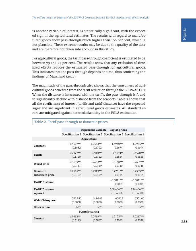
283
Nig
eria
The welfare impact in Nigeria of the ECOWAS Common External Tariff: A distributional effects analysis
is another variable of interest, is statistically significant, with the expect-ed sign in the agricultural estimates. The results with regard to manufac-tured goods show pass-through much higher than 100 per cent, which is not plausible. These extreme results may be due to the quality of the data and are therefore not taken into account in this study.
For agricultural goods, the tariff pass-through coefficient is estimated to be between 73 and 99 per cent. The results show that any exclusion of time-fixed effects reduces the estimated pass-through for agricultural goods. This indicates that the pass-through depends on time, thus confirming the findings of Marchand (2012).
The magnitude of the pass-through also shows that the consumers of agri-cultural goods benefited from the tariff reduction through the ECOWAS CET. When the distance is interacted with the tariffs, the pass-through is found to significantly decline with distance from the seaports. Table 2 shows that all the coefficients of interest (tariffs and tariff-distance) have the expected signs and are significant in agricultural goods estimates. All standard er-rors are mitigated against heteroskedasticity in the FGLS estimation.
Table 2 Tariff pass-through to domestic prices
Dependent variable – Log of prices
Specification 1 Specification 2 Specification 3 Specification 4
Agriculture
Constant–1.4507***
(0.1682)–1.0552***
(0.1702)–1.4960***
(0.1674)–1.0983***
(0.1694)
Tariffs0.7377***
(0.1120)0.9910***
(0.1152)0.3694**(0.1534)
0.6570***(0.1533)
World price0.3133***
(0.0141)0.2652***
(0.0149)0.3168***
(0.0140)0.2687***
(0.0148)
Domestic substitute price
0.7565***(0.0107)
0.7319***(0.0109)
0.7751***(0.0113)
0.7503***(0.0114)
Tariff*Distance–0.0011***
(0.0004)–0.0011***
(0.0004)
Tariff*Distance squared
5.08e-06***(1.12e-06)
5.24e-06***(1.12e-06)
Wald Chi-square5925.85(0.0000)
6194.61(0.0000)
6086.7(0.0000)
6351.66(0.0000)
Observation 1273 1273 1273 1273
Manufacturing
Constant6.9652***
(0.3145)7.0759***
(0.3067)6.9123***
(0.3092)7.0257***
(0.3029)
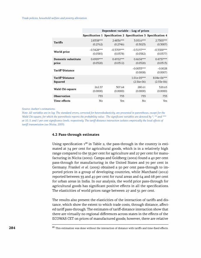
284
Trade policies, household welfare and poverty alleviation
Dependent variable – Log of prices
Specification 1 Specification 2 Specification 3 Specification 4
Tariffs2.8358***
(0.2762)2.4836***
(0.2746)3.0516***
(0.3023)2.7305***
(0.3007)
World price–0.3428***
(0.0385)–0.3709***
(0.0378)–0.3197***
(0.0382)–0.3500***
(0.0377)
Domestic substitute price
0.4909***(0.0320)
0.4952***(0.0312)
0.4654***(0.0320)
0.4737***(0.0313)
Tariff*Distance–0.0033***
(0.0008)–0.0028(0.0007)
Tariff*Distance Squared
1.01e-05***(2.56e-06)
8.04e-06***(2.55e-06)
Wald Chi-square262.57
(0.0000)307.64
(0.0000)280.61
(0.0000)320.65
(0.0000)
Observation 733 733 733 733
Time effects No Yes No Yes
Source: Author’s estimations.Note: All variables are in log. The standard errors, corrected for heteroskedasticity, are presented in parentheses, except for the Wald Chi-square, for which the parenthesis reports the probability value. The significant variables are denoted by *, ** and *** at 10, 5, and 1 per cent significance levels, respectively. The tariff-distance interaction isolates empirically the local effects of tariff transmission (see Nicita, 2009).
4.2 Pass-through estimates
Using specification 119 in Table 2, the pass-through in the country is esti-mated at 74 per cent for agricultural goods, which is in a relatively high range compared to the 33 per cent for agriculture and 27 per cent for manu-facturing in Nicita (2009). Campa and Goldberg (2002) found a 40 per cent pass-through for manufacturing in the United States and 70 per cent in Germany. Frankel et al. (2005) obtained a 50 per cent pass-through to im-ported prices in a group of developing countries, while Marchand (2012) reported between 33 and 49 per cent for rural areas and 64 and 68 per cent for urban areas in India. In our analysis, the world price pass-through for agricultural goods has significant positive effects in all the specifications. The elasticities of world prices range between 27 and 31 per cent.
The results also present the elasticities of the interaction of tariffs and dis-tance, which show the extent to which trade costs, through distance, affect-ed tariff pass-through. The estimates of tariff-distance interaction show that there are virtually no regional differences across states in the effects of the ECOWAS CET on prices of manufactured goods; however, there are relative
19 This estimation was done without the interaction of distance with tariffs and time-fixed effects.

285
Nig
eria
The welfare impact in Nigeria of the ECOWAS Common External Tariff: A distributional effects analysis
regional differences with regard to prices of agricultural goods. This result is different from Nicita (2009), who found regional differences in manufac-tured goods but no differences across states in agricultural goods. The tariff pass-through for agricultural goods prices is statistically significant, indi-cating that the tariff reduction is significantly transmitted to consumers across states through lower prices of agricultural goods. In other words, the consumers of agricultural goods benefited from the ECOWAS CET.
States closer to ports are found to be more exposed to the impact of chang-es in agricultural tariffs. Considering the state/regional differences, the tar-iff pass-through at the border is 66 per cent for the agricultural sector and it declines to 11 per cent at 100 kilometres from the port or border of en-try.20 The decline in the tariff pass-through as one gets farther away from ports of entry or borders is due to the associated trade costs, inadequate trade facilitation, and, most importantly, the poor state of infrastructure, which reduce household consumption gains from the tariff reduction and income loss for producers. The results for manufactured goods go in the same direction.21 However, possibly due to the quality of the available data, the estimates are out of a plausible band, which does not allow for a con-sistent interpretation.
The transmission of tariffs to domestic prices varies marginally across states. Table A2 in the Annex presents state-specific tariff elasticities that were obtained from specification 4 of Table 2.22 Results show that house-holds that are close to ports of entry benefit significantly from the tariff reduction. The relatively higher pass-through in agriculture in the Lagos and Rivers States is due to the location of functional ports of entry there. In fact, Lagos ports account for more than 70 per cent of port activities in Nigeria (Jaja, 2011). In addition, smuggling activities at the ports and borders in these states, which are the result of Nigeria’s porous borders (Adeola and Fayomi, 2012; Ohai, 2013),23 may have an effect on these elas-ticities.24 Smuggled goods, especially agricultural goods, avoid tariffs and are cheaper than tariffed goods.
20 The tariff pass-through at the border is the coefficient of tariffs in specification 4 in Table 2, while the estimate of the tariff-distance interaction gives the change in tariff pass-through for every kilometre of distance from the port or border. 21 Nicita (2009) opined that the tariff-distance square coefficient could take any sign depending on the rate of decline of the pass-through with distance. 22 The state-specific pass-through elasticities were obtained by finding the derivatives of equation (4) with respect to the tariff and then inserting the value of the coefficients from specification 4 in Table 2 before estimating it for each state. 23 This is the reason for the recent directive by the federal government (the Nigerian Customs Service) that all rice importation must now go through the seaports. 24 There are 1,497 illegal and 84 legal routes (borders) to Nigeria (Owete, 2013).

286
Trade policies, household welfare and poverty alleviation
4.3 Price-wage nexus
In linking domestic prices to wages,25 wage-price elasticities are estimated following the framework proposed by Nicita (2009). The estimating equa-tion considers product prices and worker characteristics:
ln Wijst = ∑ θr ln Pgst xg,r + liØ + Hjφ + εijst (5)
where Wijst is the observed wage of individual i in household j, state s at time t, Pgst is the price of good g26 in state s at time t, li is a vector of indi-vidual characteristics, Hj represents a vector of household attributes, θr in-dicates a dummy variable for worker skills27 and xg,r measures responses of wages of skilled and unskilled workers to prices.
The wages are individual monthly wages as observed in the household surveys. The control variables are age, level of education, gender, region (rural and urban), and occupation sector.28 The consumer prices from the tariff pass-through are used in the wage equation. The wages of individu-als between the age of 15 to 65 were used. In the estimation, the reference categories are the construction sector for occupation, female for gender, rural for region, and first degree holder for education. The state- and year-fixed effects are included in the regression to control for state and year specific effects. The construction of the aggregate price was based on the average prices of the basket of agricultural and manufacturing products, in line with Nicita (2009). The results of the relationship between prices of agricultural and manu-factured goods and wages are presented in Table 3. The table shows the estimates of wage-price elasticities under two different specifications of equation (5): without state- and time-fixed effects in specification 1, and with state- and time-fixed effects as in Nicita (2009) in specification 2. These estimations are carried out using the FGLS in order to fit the panel
25 The wages were obtained from the surveys and included all members of households that engaged in either farm or non-farm economic activities for wage income. NBS (2012a) reports that about 80 per cent of urban families earn income from non-farm business activities, while about 60 per cent of agricultural households also have non-farm enterprise earnings. 26 A composite agricultural good and a composite manufactured good are used in this analysis. 27 Wage earners with nine or more years of education are regarded as skilled. 28 Ten different education levels were considered: no education, primary, junior secondary, senior secondary, technical, grade II, ordinary national diploma, higher national diploma, first degree, and postgraduate degree. The occupation sectors include agriculture, manufacturing, commerce, services, transport, and construction.
gsr

287
Nig
eria
The welfare impact in Nigeria of the ECOWAS Common External Tariff: A distributional effects analysis
29 It allows estimations in the presence of the AR(1) autocorrelation within panels and cross-sectional correlation and heteroskedasticity across panels.
data linear model.29 Age, highest education attained, gender, region and sector of occupation of the workers are used as the control variables. The state-fixed effects in this framework account for the productivity differen-tial across the states due to each state’s policy specificities.
Dependent variable - Log of wage
Specification 1 Specification 2
Constant6.4145***
(0.3075)6.6170***
(0.3471)
Manufacturing price skilled0.0150
(0.0329)0.0017
(0.0323)
Manufacturing price unskilled0.0095
(0.0366)0.0119
(0.0360)
Agriculture price skilled–0.0171(0.0115)
–0.0140(0.0149)
Agriculture price unskilled0.0065
(0.0168)0.0139
(0.0165)
Age0.0633*(0.0358)
0.0280(0.0365)
Agriculture–0.2002**
(0.0820)–0.1140(0.0819)
Manufacturing0.0002
(0.0982)0.0828
(0.0984)
Commerce–0.0553(0.0883)
0.0037(0.0847)
Services0.0571
(0.0831)0.1038
(0.0829)
Transport0.1505
(0.1068)0.1955*(0.1061)
Sex0.1326***
(0.0280)0.1098***
(0.0281)
Region0.1162***
(0.0299)0.0670**(0.0322)
No education –0.9740***
(0.3511)–1.0326***
(0.3457)
Primary–0.7931**
(0.3511)–0.8772***
(0.3448)
Table 3 Wage-price elasticities

288
Trade policies, household welfare and poverty alleviation
Dependent variable - Log of wage
Specification 1 Specification 2
Junior secondary–0.6736***
(0.1714)–0.7150***
(0.1692)
Senior secondary–0.3189(0.2194)
–0.3041(0.2163)
Technical–0.5633***
(0.1666)–0.6047***
(0.1643)
Grade II–0.3974**
(0.1698)–0.4262***
(0.1674)
Ordinary national diploma0.1613
(0.2409)–0.1121(0.2422)
Higher national diploma–0.1482(0.1720)
–0.1630(0.1692)
Postgraduate–0.3677(0.4029)
–0.2975(0.3958)
Wald Chi-square481.74
(0.0000)546.87
(0.0000)
Observation 8780 8780
State-fixed effects No Yes
Time-fixed effects No Yes
Source: Author’s estimations.Note: All variables except the dummies are in log. The standard errors are presented in parentheses except for the Wald Chi-square, for which the parenthesis reports the probability value. The error term is free from autocorrelation. Skill takes the value of 1 when the worker has at least a secondary education, otherwise it is zero. Sex is 0 for female and 1 for male. The estimation uses female, construction occupation, rural and first degree holders as references.
The estimates from Table 3 show that the coefficients of many of the con-trol variables are significant, with the majority having the expected signs. Wages tend to increase with education and age. For education, all coeffi-cients have the expected signs, except for ordinary national diploma and postgraduate degree, but are non-significant. Wages also tend to be high-er for male workers and for workers in urban areas. There is a difference in the coefficient controlling for occupation, as lower wages are found in ag-riculture, while the highest wages are in transport occupations.
In general, the results show a positive correlation between manufactur-ing and agricultural prices and wages, except for the interaction of agri-cultural prices and skilled labour that is negative. The results also indicate that skilled wages are more responsive to manufacturing prices when state- and time-fixed effects are not included in the estimation. However, with state- and time-fixed effects, unskilled wages are more responsive. Skilled wages are also more responsive to agricultural prices. There are few dif-ferentials in wages between states over time in the manufacturing sector

289
Nig
eria
The welfare impact in Nigeria of the ECOWAS Common External Tariff: A distributional effects analysis
and virtually none in agriculture. This implies that there are virtually no state-specific peculiarities that influence wages. Thus, the result shows that there is no significant relationship between prices and wages,30 indicating that the nexus between prices and wages is not established in this study.
4.4 Welfare impact
The empirical analysis in this sub-section examines the impact of the ECOWAS CET on Nigerian households by focusing on the price changes of traded goods and wage income. The specific results regarding the welfare effects of trade liberalization in geopolitical zones and states are present-ed in Table A2 in the Annex.
In Nigeria, many households are simultaneously wage earners, produc-ers and consumers of goods. It is therefore important to recognize these roles when analysing the impact of any policy on household welfare.31 The share of wages in the income of most households is small compared to the income from sales of agricultural and manufactured goods. In ru-ral areas, agricultural sales often constitute the bulk of the household in-come. This income is then increased through wages earned from labour rendered by the members of the household in other farm or non-farm ac-tivities.32 However, in urban areas, income from manufacturing sales and wages represents the most important component of household income. Expenditure on agricultural products, especially food items, often forms the bulk of household expenses.
Following Porto (2006), Nicita (2009), and Marchand (2012), this study es-timates the effects of trade policy on household welfare. It indicates that changes in utility dUhs of household h in state s depend on the changes in local prices (both goods and factors), household-specific labour income, ag-ricultural production, and consumption. This relation is presented in equa-tion (6).
dUhs = ∑θ rh dWsr + ∑θ xhg dPgs – ∑θ chg dPgs (6)
where θ chg is the income share spent on good g by household h, θ xhg is the income share obtained from selling goods produced at price P, θ rh is the
30 This could be due to rigidity on the part of employers in adjusting wages, even in the presence of price changes. Also, the country’s minimum wages determined by the federal government tend not to react fast to price changes. 31 See Singh et al. (1986) for the farm household model, a standard model which is often used to measure changes in households’ welfare. 32 The largest proportion of Nigeria’s labour is in the agricultural sector (IFAD, 2012).
r g g

290
Trade policies, household welfare and poverty alleviation
income share earned from labour, and dPgs and dWsr are changes in prices
and wages, respectively. Aggregate welfare change is therefore given by the sum of the welfare changes of all households. Thus, households’ ex-posure to changes in prices and wages will depend on their income struc-ture and expenditure allocation. The calculation for each household was done taking into consideration expenditure and income, the different types of labour supplied (skilled and unskilled), and the fact that the price ef-fects estimations vary among states. Aggregating the results across house-holds, the study finds that the effects of the ECOWAS CET on households in Nigeria vary both across income groups and states. This is due to the differences in economic behaviours, endowments and pass-through across the states. Due to the insignificance of the wage elasticities, this analysis only considers the effects of price changes on welfare.
Earlier results indicated that tariff liberalization led to price reductions in both agricultural and manufactured goods. Unskilled and skilled wages in both sectors remained basically unchanged after trade liberalization. Some selected details about the impact of the ECOWAS CET are presented in Table A2 in the Annex. It can be seen that the CET has resulted in an increase of overall household welfare of 6.9 per cent at the national level. The gains originate from the expenditure basket (8.9 per cent), which compensated for the losses incurred by households from sales of agricultural goods (1.9 per cent). Disaggregating the effects indicates that there are differences across geopolitical zones and states as well as between rural and urban areas.
In terms of the geographical distribution of welfare gains due to the CET, the analysis finds that households in the northern states have benefited more than those in the southern states, due to higher expenditure gains. Furthermore, the overall change in real income due to the CET in the ag-ricultural sector indicates that the producers in this sector have been ad-versely affected due to the generally high level of pass-through. Although the CET has negatively affected the producers of agricultural products, consumers of agricultural products have been better off due to the availa-bility of wider variety of cheaper goods.
This study also finds that the effects of the CET vary along the income distribution. The mean expenditure gains across income percentiles are shown in Figure 1.33 On average, all household income groups have expe-rienced expenditure gains, but to varying degrees.
33 The figure shows changes in real income due to changes in expenditure, agricultural and manufacturing sales.

291
Nig
eria
The welfare impact in Nigeria of the ECOWAS Common External Tariff: A distributional effects analysis
Figure 2 shows average total gains. All income groups have benefited from trade liberalization, and households at lower income levels have ex-perienced higher welfare gains. It can be seen from the figure that all households have benefited from lower expenditure due to lower prices, with those in the 80th and 100th percentiles gaining less and those in the lowest income percentile gaining the most. Thus, the poorest house-holds in Nigeria on average have benefitted more from the CET than the richest households, due to a greater share of agricultural goods in their expenditure basket. High-income households have experienced lower wel-fare gains due to the small share of agricultural commodities in their ex-penditure. The real income of households has changed due to the fact that agricultural sales have been negative for households relying mostly on sales of these products.
Figure 1 Changes in real income
Source: Author’s estimations.
― Total gains
― Expenditures
Agricultural sales
Cha
nge
in r
eal i
ncom
e
Income percentiles
-5
0 20 40 60 80 100
0
5
10

292
Trade policies, household welfare and poverty alleviation
5 Conclusions
This study examined the extent to which households have been affect-ed by the Common External Tariff of the Economic Community of West African States. The empirical analysis examined economic consequences of the CET from the perspective of households as producers, consumers and workers, as well as the transmission of the tariff reduction under the CET to domestic prices. The results show that the ECOWAS CET has re-duced domestic prices of agricultural goods. The study did not find a signif-icant link between wages and prices. The findings also indicate that so far the CET has had a net positive effect on households in Nigeria, largely due to the gains from expenditure which outweighed the losses in the house-holds’ purchasing power due to lower income from the sales of agricultur-al products. Consequently, household welfare has improved as a result of the CET, particularly for poor households in rural areas; the gains for high-er-income households have been more modest. Some groups of house-holds whose income depend largely on activities in the agricultural sector, specifically product sales, have seen a depletion of their purchasing power.
Despite the overall net positive effects of the CET, the study finds differ-ences in the distribution of welfare gains across states, geopolitical zones and income groups. Richer households have experienced lower welfare gains than poorer households. The welfare gains of urban households and male-headed households have been higher than those of rural households and female-headed households, respectively. Rural households in states
34 This would include labour market reforms.
Figure 2 Total gains
Cha
nge
in r
eal i
ncom
e
Income percentiles
5
0 20 40 60 80 100
6
7
8
9
Source: Author’s estimations.

293
Nig
eria
The welfare impact in Nigeria of the ECOWAS Common External Tariff: A distributional effects analysis
with ports of entry and near borders have seen their purchasing power eroded more than households in urban areas. Consumers in states with ports of entry have been more exposed to goods available at relatively low-er prices due to the CET than those in other states. Thus, the study provides evidence that domestic price transmission, household characteristics, and sectors of economic activity are significant in assessing the welfare effects of trade policies in Nigeria.
This study provides relevant findings about welfare implications of the ECOWAS CET which could serve in the formulation of Nigeria’s nation-al economic transformation agenda in the areas of trade and investment, agricultural productivity, and wealth and job creation.34 The capacity of producers should be enhanced through an informed, integrated and in-clusive policy for both the manufacturing and agricultural sectors that would stimulate productivity and value addition. The government should boost investment in vital sectors of the economy by improving infrastruc-ture, access to finance and quality of education, promoting science and technology, facilitating land acquisition, etc. For instance, the Commercial Agriculture Development Programme, as well as other programmes of the Ministry of Agriculture and Rural Development, should be reinforced. This could enhance the competitiveness of domestic producers and increase the volume of output, employment and income levels.
Policy measures are also needed to mitigate the domestic effects of gov-ernment trade policies. In this context, the National Poverty Eradication Programme, the National Directorate of Employment’s Programme, the Subsidy Reinvestment and Empowerment Programme, and other rele-vant government programmes should be strengthened to create jobs and wealth in agriculture and the manufacturing sector. Social safety nets and security measures should also be put in place at the rural level, especial-ly for vulnerable populations, in order to mitigate the negative income ef-fects of the CET on rural households.35
Finally, efforts could also be made to reduce the number of banned prod-ucts, as such import bans may have the tendency to encourage smuggling because some of the banned goods are in demand given their limited do-mestic production. This leads to a situation whereby government bans, while trying to protect domestic producers, result in a proliferation of il-legal/informal importation.
35 The National Poverty Eradication Programme could liaise with the Ministries of Youth and Women’s Affairs to come to the aid of vulnerable populations by empowering them economically.

294
Trade policies, household welfare and poverty alleviation
Agriculture Manufacturing
2006 2007 2009 2011 2006 2007 2009 2011
Abia5.386
(1.201)5.418
(1.160)5.580
(1.145)5.738
(1.270)5.375
(0.645)5.509
(0.671)5.731
(0.583)5.902
(0.614)
Adamawa5.205
(1.256)5.143
(1.373)5.413
(1.150)5.559
(1.266)5.389
(0.631)5.468
(0.640)5.678
(0.638)5.778
(0.602)
Akwalbom5.419
(1.182)5.445
(1.165)5.615
(1.125)5.861
(1.258)5.470
(0.648)5.555
(0.673)5.714
(0.624)5.858
(0.595)
Anambra5.274
(1.105)5.380
(1.166)5.616
(1.232)5.712
(1.251)5.430
(0.625)5.473
(0.632)5.647
(0.582)5.817
(0.571)
Bauchi5.118
(1.373)5.082
(1.332)5.352
(1.190)5.900
(1.336)5.429
(0.700)5.474
(0.651)5.570
(0.579)5.769
(0.594)
Bayelsa5.708
(1.226)5.473
(1.038)5.612
(1.063)5.871
(1.393)5.436
(0.597)5.599
(0.471)5.680
(0.623)5.900
(0.621)
Benue5.151
(1.276)5.178
(1.423)5.427
(1.229)5.722
(1.393)5.422
(0.652)5.465
(0.631)5.681
(0.592)5.837
(0.601)
Borno5.187
(1.394)5.169
(1.396)5.337
(1.230)5.516
(1.189)5.399
(0.646)5.417
(0.588)5.591
(0.579)5.812
(0.608)
Cross River5.405
(1.173)5.362
(1.129)5.522
(1.124)5.847
(1.184)5.456
(0.654)5.532
(0.655)5.688
(0.610)5.870
(0.604)
Delta5.289
(1.070)5.432
(1.110)5.587
(1.039)5.812
(1.196)5.389
(0.642)5.509
(0.666)5.864
(0.772)5.852
(0.610)
Ebonyi5.241
(1.070)5.320
(1.155)5.594
(1.120)5.761
(1.127)5.432
(0.665)5.486
(0.666)5.646
(0.587)5.778
(0.593)
Edo5.417
(1.078)5.461
(1.112)5.568
(1.150)5.821
(1.223)5.398
(0.598)5.468
(0.610)5.711
(0.628)5.821
(0.589)
Ekiti5.245
(1.170)5.312
(1.296)5.657
(1.357)5.698
(1.253)5.237
(0.760)5.512
(0.652)5.646
(0.561)5.821
(0.576)
Enugu5.252
(1.194)5.390
(1.263)5.612
(1.171)5.635
(1.246)5.369
(0.613)5.398
(0.595)5.657
(0.601)5.785
(0.576)
Gombe5.016
(1.284)5.120
(1.396)5.345
(1.226)5.546
(1.298)5.394
(0.634)5.418
(0.637)5.575
(0.616)5.741
(0.574)
Imo5.356
(1.067)5.374
(1.157)5.534
(1.186)5.901
(1.321)5.430
(0.630)5.418
(0.605)5.658
(0.598)5.846
(0.584)
Jigawa4.840
(0.965)4.952
(1.246)5.298
(1.189)5.486
(1.184)5.505
(1.883)5.371
(0.619)5.671
(0.627)5.787
(0.591)
Kaduna4.898
(1.099)5.067
(1.377)5.423
(1.289)5.635
(1.353)5.362
(0.609)5.391
(0.613)5.598
(0.589)5.775
(0.580)
Table A1 Domestic prices by year and state, 2006–2011 (log)
Annex

295
Nig
eria
The welfare impact in Nigeria of the ECOWAS Common External Tariff: A distributional effects analysis
Kano5.025
(1.291)4.984
(1.338)5.432
(1.396)5.537
(1.270)5.735
(1.210)5.863
(1.390)5.728
(0.637)5.912
(0.683)
Katsina5.023
(1.231)5.052
(1.309)5.384
(1.304)5.591
(1.371)5.401
(0.750)5.332
(0.620)5.614
(0.623)5.912
(0.683)
Kebbi5.143
(1.216)5.084
(1.288)5.397
(1.185)5.598
(1.285)5.308
(0.643)5.400
(0.649)5.582
(0.568)5.790
(0.575)
Kogi5.098
(1.100)5.132
(1.180)5.632
(1.261)5.777
(1.293)5.382
(0.624)5.438
(0.620)5.651
(0.590)5.838
(0.598)
Kwara5.127
(1.302)5.141
(1.376)5.481
(1.254)5.699
(1.344)5.342
(0.596)5.464
(0.605)5.637
(0.578)5.838
(0.592)
Lagos5.269
(1.108)5.361
(1.184)5.658
(1.233)5.780
(1.237)5.355
(0.632)5.446
(0.619)5.646
(0.569)5.793
(0.589)
Nasarawa5.212
(1.393)5.158
(1.445)5.472
(1.284)5.701
(1.460)5.398
(0.653)5.436
(0.616)5.603
(0.561)5.885
(0.627)
Niger5.104
(1.266)5.131
(1.332)5.385
(1.180)5.618
(1.318)5.383
(0.638)5.483
(0.618)5.601
(0.545)5.782
(0.578)
Ogun5.128
(1.130)5.245
(1.246)5.583
(1.180)5.730
(1.201)5.342
(0.601)5.378
(0.607)5.582
(0.551)5.786
(0.569)
Ondo5.219
(1.234)5.278
(1.282)5.514
(1.197)5.721
(1.238)5.399
(0.604)5.461
(0.608)5.631
(0.575)5.852
(0.572)
Osun5.218
(1.301)5.216
(1.408)5.465
(1.256)5.648
(1.301)5.337
(0.610)5.456
(0.636)5.624
(0.551)5.82
(0.587)
Oyo5.169
(1.285)5.175
(1.326)5.480
(1.231)5.668
(1.318)5.368
(0.616)5.513
(0.627)5.665
(0.593)5.811
(0.605)
Plateau5.177
(1.311)5.143
(1.411)5.577
(1.338)5.669
(1.345)5.368
(0.643)5.468
(0.619)5.714
(0.611)5.873
(0.631)
Rivers5.438
(1.186)5.422
(1.179)5.633
(1.155)5.841
(1.242)5.460
(0.651)5.530
(0.649)5.688
(0.604)5.868
(0.609)
Sokoto5.371
(1.461)5.068
(1.119)5.454
(1.155)5.652
(1.307)5.353
(0.616)5.433
(0.649)5.593
(0.576)5.737
(0.554)
Taraba4.822
(1.225)5.172
(1.375)5.336
(1.136)5.609
(1.281)5.450
(0.614)5.406
(0.653)5.624
(0.609)5.762
(0.579)
Yobe5.023
(1.138)5.105
(1.238)5.420
(1.242)5.711
(1.400)5.391
(0.617)5.482
(0.654)5.581
(0.586)5.730
(0.516)
Zamfara5.101
(1.292)4.993
(1.273)5.354
(1.200)5.604
(1.343)5.312
(0.618)5.188
(0.830)5.631
(0.621)5.852
(0.624)
Federal Capital Territory/Abuja
5.133(1.265)
5.252(1.368)
5.585(1.317)
5.769(1.443)
5.372(0.642)
5.578(0.643)
5.678(0.611)
5.810(0.599)
National5.195
(1.171)5.222
(1.219)5.496
(1.155)5.585
(1.161)5.408
(0.604)5.467
(0.606)5.651
(0.541)5.818
(0.534)Source: Author’s estimations.Note: Prices are expressed in nominal terms. Nominal domestic prices are the unit values that were sourced from NBS commodity prices and averaged across the states. Variances are shown in parentheses. Rice, maize, sorghum, chicken, soya beans, meat, fish, groundnut, oranges, and shrimps were used for agricultural commodities, while manufactured products consist of processed items.

296
Trade policies, household welfare and poverty alleviation
Pass-through
Income share
Expenditure share
Changes in real income due to
Overall changes
in real income due to the CET
Agr
icul
ture
Agr
icul
ture
Man
ufac
turi
ng
Agr
icul
ture
Man
ufac
turi
ng
Agr
icul
tura
l sa
les
Con
sum
ptio
n ex
pend
itur
e
Tota
l
North-Central – 7.3 72.5 62.8 36.4 –1.8 11.5 9.7
Benue 44.07 23.03 69.82 60.87 38.19 –7.99 21.11 13.12
Kogi 43.98 4.43 81.79 67.86 31.67 –1.48 22.72 21.23
Kwara 46.40 13.09 83.12 66.68 32.56 0.00 0.00 –0.41
Nasarawa 44.30 0.04 45.57 69.66 29.79 0.00 8.39 8.38
Niger 45.45 0.02 90.22 66.06 33.55 0.00 2.56 2.56
Plateau 50.22 2.20 56.42 59.07 39.69 –0.70 18.73 18.03
Federal Capital Territory
47.10 3.48 55.42 46.05 52.62 –0.26 3.40 3.14
North-East – 17.1 73.7 66.9 31.8 –4.4 15.5 11.1
Adamawa 51.99 27.13 72.86 64.72 34.63 –8.80 20.98 12.19
Bauchi 56.08 2.72 74.80 64.2 32.87 –0.36 8.49 8.13
Borno 141.49 20.11 76.31 74.23 24.87 –4.39 16.20 11.81
Gombe 88.4 27.7 55.60 63.75 35.88 –5.75 13.25 7.49
Taraba 53.97 25.58 58.35 79.89 18.70 –7.23 22.58 15.35
Yobe 86.38 7.26 92.72 53.66 45.89 –1.70 13.90 12.02
North-West – 9.3 75.5 71.0 28.5 -0.4 11.9 10.2
Jigawa 77.25 7.33 79.20 66.76 33.11 -0.70 6.39 5.69
Kaduna 52.19 14.49 66.33 66.10 33.10 –3.42 15.58 12.16
Kano 71.16 6.17 73.94 78.12 21.47 –1.03 13.02 11.99
Katsina 74.59 0.02 86.86 59.58 40.16 0 11.66 11.65
Kebbi 54.80 14.88 85.07 76.59 22.49 –1.00 5.14 4.14
Sokoto 62.72 21.88 70.53 67.18 32.67 –6.93 21.29 14.35
Zamfara 59.78 11.40 60.87 87.34 11.81 1.40 10.76 9.36
South-East – 15.4 65.6 58.1 40.6 –0.9 2.9 2
Abia 56.17 1.98 66.78 52.22 46.03 –0.07 1.95 1.88
Anambra 13.13 24.36 66.9 62.68 36.49 –0.67 1.73 1.06
Ebonyi 48.69 0.01 79.1 36.58 63.01 0 0.35 0.35
Enugu 44.49 12.82 56.65 54.96 42.14 –0.28 1.21 0.93
Imo 58.06 24.85 58.92 72.18 26.41 –2.52 7.32 4.80
South-South – 12.6 61.7 59.8 39.0 -3.3 11.8 8.4
AkwaIbom 55.44 10.89 32.41 59.21 38.90 –1.98 10.75 8.78
Table A2 Overview of results, 2006–2011 (per cent)

297
Nig
eria
The welfare impact in Nigeria of the ECOWAS Common External Tariff: A distributional effects analysis
Figure A1 Geopolitical zones of Nigeria
Source: Author’s calculations.
Source: Nairaland, available at: http://www.nairaland.com/359384/scrap-36-states-now-anyaoku/3.
Pass-through
Income share
Expenditure share
Changes in real income due to
Overall changes
in real income due to the CET
Agr
icul
ture
Agr
icul
ture
Man
ufac
turi
ng
Agr
icul
ture
Man
ufac
turi
ng
Agr
icul
tura
l sa
les
Con
sum
ptio
n ex
pend
itur
e
Tota
l
Bayelsa 57.53 49.1 44.38 64.28 33.83 –24.81 33.16 8.35
Cross River 52.54 15.43 84.59 61.39 36.61 –2.19 8.70 6.51
Delta 51.86 17.97 82.01 61.06 37.92 –3.29 11.19 7.90
Edo 46.82 1.61 81.54 63.81 35.52 –0.28 11.14 10.86
Rivers 65.37 4.18 53.76 55.34 44.17 –0.70 9.22 8.53
South-West – 8.6 81.1 56.7 42.1 0.1 1.4 1.6
Ekiti 47.18 13.13 75.98 56.55 41.98 –0.36 1.54 1.18
Lagos 65.26 0.27 89.1 51.37 47.61 –0.04 7.27 7.23
Ogun 57.97 0.03 81.72 53.3 44.16 0 2.61 2.61
Ondo 48.14 20.21 78.36 65.00 34.09 –0.54 1.73 1.19
Osun 49.38 14.36 77.43 58.80 39.45 1.04 –4.24 –3.21
Oyo 54.50 8.06 79.02 56.07 42.6 0.03 –0.23 –0.20
National 59.9 11.7 71.6 62.2 36.7 –1.9 8.9 6.9
Rural – 24.9 59 79.5 19.1 –7 22 15
Urban – 11.7 71.9 61.6 37.1 –1.8 8.6 6.8
□ North-West
■ North-East
■ North-Central
■ South-West
■ South-East
■ South-South
Sokoto
ZamfaraKebbi
Kwara
Oyo
OgunLagos
OndoEdo
Delta Imo Aba
EnuguEbonyiAnambra
Bayelsa
Rivers Akwalbom
Cross River
EkitiOsun
Niger
F.C.T.Abuja
KogiBenue
Nasarawa
Plateau
Katsina
Kaduna
Kano
JigawaYobe
Borno
Bauchi Gombe
Taraba
Adamawa

298
Trade policies, household welfare and poverty alleviation
References
Adeola, G.L. and Fayomi,O. (2012).“The Political and Security Implication of Cross Border Migration Between Nigeria and Her Francophone Neighbours.” International Journal of Social Sciences Tomorrow, 1 (3): 1–9.
Ajayi, K. and Osafo-Kwaako, P. (2007). “Research and Trade Policy Formulation: The Case of Nigeria’s Adoption of the ECOWAS Common External Tariffs (CET).” LATN Working Paper No. 78 (July). Latin America Trade Network, Buenos Aires.
Balogun, E.D. and Dauda, R.O. (2012). “Poverty and Employment Impact of Trade Liberalization in Nigeria: Empirical Evidence and Policy Implications.” University of Lagos.
Campa, J.M. and Goldberg, L.S. (2002). “Exchange Rate Pass-Through into Import Prices: A Macro or Micro Phenomenon?” NBER Working Paper No. 8934. National Bureau of Economic Research, Cambridge MA.
Castilho, M., Menendez, M. and Sztulman, A. (2012). “Trade Liberalization, Inequality, and Poverty in Brazilian States.” Poverty and Social Exclusion Working Paper No. 2009–33. Paris School of Economics.
ECOWAS Vanguard (2013). “The ECOWAS Trade Liberalization Scheme: Genesis, Conditions and Appraisal.” ECOWAS Vanguard, 2 (3). NANTS Regional Trade Advocacy Series. National Association of Nigerian Traders, Abuja.
Frankel, J.A., Parsley, D.C. and Wei, S.J. (2005). “Slow Pass-Through Around the World: A New Import for Developing Countries?” Research Working Paper No. RWP05-016. John F. Kennedy School of Government Faculty, Harvard University.
Goldberg, P.K. and Pavcnik, N. (2003). “The Response of the Informal Sector to Trade Liberalization.” Journal of Development Economics, 72 (2): 463–496.
Goldberg, P.K. and Pavcnik, N. (2007). “Distributional Effects of Globalization in Developing Countries.” Journal of Economic Literature, 45 (1): 39–82.
IFAD (2012). “Message Delivered on Behalf of IFAD President at Golden Jubilee Anniversary Lecture: Revamping Nigeria’s Agriculture [online].” International Fund for Agricultural Development, Rome. Available at: http://www.ifad.org/events/op/2012/nigeria.htm.
IMF (2013). Direction of Trade Statistics database [online]. International Monetary Fund, Washington DC. Available at:http://elibrary-data.imf.org/FindDataReports.aspx?d=33061&e=170921.
Jaja, C.Y. (2011). “Freight Traffic at Nigeria’s Seaports: Problems and Prospect.” The Social Sciences, 6 (4): 250–258.
Kuji Ltd. (2002). “Comprehensive Review of the Nigerian Customs and Excise Tariff 1995 – 2001: Implications for Nigeria of The ECOWAS Common External Tariff and Nigeria’s Obligations/commitments under WTO, ECOWAS, AGOA AND ACP-EU.” Report to the Federal Ministry of Finance.
Marchand, B.U. (2012). “Tariff Pass-through and the Distributional Effects of Trade Liberalization.” Journal of Development Economics, 99 (2): 65–281.
Marchat, J.M. and Rajhi, T. (2004). “Estimates of the Impact of a Common External Tariff on the Nigerian Manufacturing Sector: Some Simulation Results Based on Firm Level Data.” Working Paper. Paris and Washington DC: University of Paris I and World Bank.
Martinez, G.M. and Poole, N. (2004). “The Development of Private Fresh Produce Safety Standards: Implications for Developing Mediterranean Exporting Countries.” Food Policy, 29 (3): 229–255.

299
Nig
eria
The welfare impact in Nigeria of the ECOWAS Common External Tariff: A distributional effects analysis
McCaig, B. (2011). “Exporting out of Poverty: Provincial Poverty in Vietnam and U.S. Market Access.” Journal of International Economics, 85 (1): 102–113.
NBS (2012a). Consumption Pattern in Nigeria 2009/10: Preliminary Report. 2009/10 Consumption Report, March. National Bureau of Statistics of Nigeria.
NBS (2012b). Social Statistics in Nigeria 2012 – Part III (Health, Employment, Public Safety, Population and Vital Regulation) [online]. National Bureau of Statistics of Nigeria. Available at: www.nigerianstat.gov.ng.
Nicita, A. (2004). “Who Benefited from Trade Liberalization in Mexico? Measuring the Effects on Household Welfare.” Policy Research Working Paper No. 3265. World Bank, Washington DC.
Nicita, A. (2009). “The Price Effect of Tariff Liberalization: Measuring the Impact on Household Welfare.” Journal of Development Economics, 89 (1): 19–27.
Nwafor, M. (2006). “Trade Liberalization and Poverty in Nigeria: Lessons from the Past.” African Institute for Applied Economics, now African Heritage Institution, Enugu.
Nwafor, M., Ogujiuba, K. and Adenikinju, A. (2005). “The Impact of Trade Liberalization on Poverty in Nigeria: Micro Simulation in a CGE Model.” Interim Report to the Poverty and Economic Policy (PEP) Research Network. Paper pre-sented during the 4th PEP Research Network General Meeting. Colombo, 13–17 June.
Oduh, M.O. (2012). “Trade Openness and Output Variability in Nigeria: Implications for EU-ACP Economic Partnership Agreement.” Developing Country Studies, 2 (7): 73–83.
Ohai, Chux. (2013). “Seme Border: From Benin to Nigeria on Fabricated Vespa.” Punch [online], 28 February. Available at: http://www.punchng.com/feature/seme-border-from-benin-to-nigeria-on-fabricated-vespa/.
Owete, F. (2013). “Nigeria Has 1,497 Illegal Borders.” Premium Times [online], 23 May. Available at: http://www.premium-timesng.com/news/135901-nigeria-has-1497-illegal-borders-interior-minister.html.
Oyejide, A. (2012). “The impact of the ECOWAS CET on the real sector: a case study of the manufacturing sector.”
Porto, G. (2006). “Using Survey Data to Assess the Distributional Effects of Trade Policy.” Journal of International Economics, 70 (1): 140–160.
Soludo, C. and Oji, E. (2003). “Does Trade Openness Make Sense at This Time in Nigeria?” Paper prepared for the TRADEMAC Trade and Macroeconomic Working Group.
Topalova, P. (2005). “Trade Liberalization, Poverty and Inequality: Evidence from Indian Districts.” NBER Working Paper No. 11614. National Bureau of Economic Research, Cambridge MA.
Topalova, P. (2010). “Factor Immobility and Regional Impacts of Trade Liberalization: Evidence on Poverty from India.” America Economic Journal, 2 (4): 1–41.
UNCTAD (2012). Handbook of Statistics. United Nations publication. Sales No. B.12.II.D.1. New York and Geneva. Available at: http://unctad.org/en/pages/PublicationWebflyer.aspx?publicationid=381.
Urama, N.E., Nwosu, E.O. and Aneke, G.C. (2012). “Lost Revenue Due to Trade Liberalization: Can Nigeria Recover Her Own?” European Journal of Business and Management, 4 (10): 134–142.
World Bank (1996). Nigeria: The Challenges of Growth with Inclusion. World Bank, Washington DC.

300
Trade policies, household welfare and poverty alleviation
Viet Nam

301
Vie
t N
am
Household welfare and pricing of rice: Does the Large-Scale Field Model matter for Viet Nam?
Abstract
Since 2006, Viet Nam’s rice exports have soared, and in 2011 the coun-try surpassed Thailand to become the world’s largest rice exporter. Even though one would expect higher rice exports to directly benefit rural households at all levels of well-being, most rice producers in Viet Nam are still poor, living on less than USD 2 per day. The government’s ef-forts to ensure a minimum rate of return for farmers by imposing price floors (minimum prices) have not been successful, as there is no enforce-ment mechanism in place. This study examines the potential impact on household welfare in Viet Nam of value chain upgrading in rice produc-tion through the Large-Scale Field Model. The possible effects of the adop-tion of such a model are: (a) an increase in the farm gate price of rice, (b) an increase in the productivity of rice farmers, and (c) a reduction in farmers’ production costs. The study shows how these changes would affect house-hold welfare, taking into account the ripple effect that a change in the farm gate price of rice would have on other prices in the economy, and hence on household consumption, production, and wage income. The policy simula-tions in this study assume that farmers do not pass on any cost reductions and productivity improvements to the price of paddy. The results suggest that the implementation of the Large-Scale Field Model in the Mekong River Delta would increase the welfare of households by 4.1 per cent in the short term and 4.9 per cent in the longer term, and reduce poverty rates by approximately 0.55 per cent among the 10 per cent poorest households and by 0.42 per cent among the 20 per cent poorest households in that region.
* The authors would like to thank Dang Kim Son and Tran Cong Thang from the Institute of Policy and Strategy for Agriculture and Rural Development, and Bui Trinh from the General Statistics Office of Viet Nam, for their support in the preparation of this study.
Ngoc Quang Pham and Anh Hai La *

302
Trade policies, household welfare and poverty alleviation
1 Introduction
Doi Moi, a Vietnamese term meaning “renovation”, marked the beginning of Viet Nam’s transition from a centrally planned to a more market-driv-en economy. Initiated by the Communist Party Congress in 1986, Doi Moi became a major phenomenon in Viet Nam during 1986–1990. Its main aim was to promote a multi-sectoral economic system encompassing both state-owned and private enterprises. In the framework of the Doi Moi pol-icy, state-owned enterprises were reformed, private sector enterprises and companies with foreign investment emerged de novo, and the domes-tic market was liberalized to allow for free market prices. In agriculture, Politburo Resolution No. 10 made it possible to conclude “end-product contracts” with households; and land use rights were granted for 15 years in 1988, a period further extended to 20 years in 1993 (Pham et al., 2007).
One of the most striking features of Viet Nam’s transition was a high growth rate of the gross domestic product (GDP), coupled with a remarka-ble increase in exports. Before the Doi Moi, Viet Nam had to import food for domestic consumption. After the agricultural reforms in 1988, agricultur-al output rose tremendously and in 1989, Viet Nam became a rice export-er (Pham et al., 2007). The value of the country’s rice exports has soared particularly since 2006 (Figure 1). In 2011, Viet Nam surpassed Thailand to become the world’s largest rice exporter, with more than 7 million met-ric tons of rice exported, of which 95 per cent was contributed by farmers – net rice producers – in the Mekong River Delta (Jaffee, 2012a).
Figure 1 Viet Nam’s rice exports, 1989–2011
8
7
6
5
4
3
2
1
0
4,000
3,500
3,000
2,500
2,000
1,500
1,000
500
0
Mill
ions
of
met
ric
tons
Nom
inal
tho
usan
ds o
f U
SD
1989
1990
1991
1992
1993
1994
1995
1996
1997
1998
1999
2000
2001
2002
2003
2004
2005
2006
2007
2008
2009
2010
2011
■ Volume (LHS) ― Value (RHS)
Source: Authors’ calculations, based on data from the Vietnam Food Association (VFA, 2006) and General Statistics Office (GSO) of Viet Nam.Note: LHS stands for left-hand scale, RHS for right-hand scale.

303
Vie
t N
am
Household welfare and pricing of rice: Does the Large-Scale Field Model matter for Viet Nam?
Although higher rice exports could be expected to directly benefit rural households at all levels of well-being, most rice producers in Viet Nam remain poor, living on less than USD 2 per capita per day (Coxhead et al., 2012).
Viet Nam’s current rice value chain, shown in Figure 2, explains the main reason for the low incomes of Vietnamese farmers. Owing to the many in-termediaries in the chain, the benefits of the remarkable increase in rice export volumes and prices have not accrued to the households that ac-tually grow the rice. As a matter of fact, 95.8 per cent of total paddy rice produced by those households is sold to collectors and (subsequently) to millers, and only 4.2 per cent is sold directly to exporters.
Figure 2 Viet Nam’s rice value chain, 2010
Source: Vo and Nguyen (2011).
Inputs:Capital stockLabourIrrigationSeedFertilizersPesticidesTechnical support
Farmers
Col
lect
ors
Mil
lers
Trad
ers/
Exp
orte
s
Dom
esti
c re
tail
ers
Poli
shin
g fa
ctor
ies
4.2%
Rice export: 70.3%
Rice domesticconsumption: 29.7%
2.7%
93.1%30.3%
47.8%
15%
21%
10.7% 3.5% 6.2%
1.3% 1.3% 1.3%
7.2% 7.2%
Collectors, who tend to participate more actively in the value chain (mill-ers or polishing factories act as service providers for collectors), earned 10 times more than farmers in 2011 (Tran et al., 2013). Having more market power than farmers, collectors usually set low prices, particularly if there is a good crop (a surplus of paddy rice supply). Additionally, as most farm-ers are poor, their biggest need for cash is in the period right after the har-vest. They therefore have to sell their output as quickly as possible and at any price (usually lower than the floor farm gate price, i.e. the minimum price set by the government) to settle their debts in time. Table 1 shows that interest payments on farmers’ loans alone account for more than 17 per cent of total costs related to rice cultivation. Another problem is the losses directly attributable to poor post-harvest technologies, which do not allow farmers to retain rice for later sale. Post-harvest losses occur as a result of the lack of storage facilities (most farmers use small storehous-es and have no storage systems), as well as inadequate paddy drying tech-nology. To save on costs, most farmers prefer sun drying. However, as sun

304
Trade policies, household welfare and poverty alleviation
drying is associated with a number of technical constraints,1 most farm-ers sell their wet paddy to collectors at considerably lower prices because longer delays mean a higher water loss, which causes shrinkage and loss of weight of their wet paddy harvest.2
Over the past five years, the Vietnamese government has experimented with a number of price policy instruments aimed at ensuring a minimum rate of return of 30 per cent for farmers who are engaged in growing pad-dy. The main instrument consists of “floor prices” for paddy both for ex-ports (minimum export free on board (FOB) price) and for purchases from rice farmers (minimum farm gate price for paddy).3 Exporters are request-ed not to sell rice for a price lower than the floor export FOB price, the level
Table 1 Share of inputs in costs of paddy cultivation (per cent)
Source: Vo and Nguyen (2011).
Inputs Per cent
1 Seed, fertilizers, pesticides 42.4
2 Labour (self-employed) 9.6
3 Labour (hired) 20.6
4 Capital stock (including depreciation) 2.8
5 Irrigation fee 2.5
6 Interest (loan of inputs) 2.8
7 Interest (bank loan) 14.4
8 Transportation 1.6
9 Other (commission for collectors) 3.3
Total 100.0
1 First, sun drying is not possible during rain and at night, so there is a risk that farmers will not be able to dry their paddy right after harvest. Second, the process is labour-intensive and has high requirements with regard to the size of drying pavements/mats that need to be available. Third, temperature control is difficult, with a high likelihood of overheating or rewetting of grains, which in turn can result in low milling quality because of cracks developing in the kernels (IRRI, 2006). 2 According to Tran et al. (2013), only 5 per cent of farmers sell dry paddy to collectors. 3 The minimum export FOB price of rice is set based on the price of rice on the world market (Circular 89/2011/TT-BTC issued on 17 June 2011), whereas the farm gate price of paddy is set above the average production cost of paddy for each crop (Decree 109/2011/NDD-CP issued on 4 November 2010). Therefore, if the world price of rice falls, according to Circular 89/2011/TT-BTC, exporters have to maintain their profit by reducing other costs but not the farm gate price of paddy.

305
Vie
t N
am
Household welfare and pricing of rice: Does the Large-Scale Field Model matter for Viet Nam?
of which is set on the assumption that exporters would buy paddy directly from farmers for the recommended floor farm gate price.4
As shown in Figure 2, exporters (or even domestic retailers) almost never buy paddy from farmers, but rather from millers and/or polishing facto-ries. What prevents farmers from selling directly to exporters and/or do-mestic retailers?
One of the main reasons is the imperfect competition among Vietnamese rice exporters. In Viet Nam, 50 per cent of rice is exported through gov-ernment-to-government (G2G) contracts. The Vietnam Food Association has the right to allocate 80 per cent of total volume of G2G contracts to its members, which are mostly state-owned enterprises (SOEs) (Tran et al., 2013).5 As SOEs have little incentive to improve performance (Boycko et al., 1996) and G2G contracts do not require high-quality rice, these pub-lic exporters have become less active in searching for new markets or im-proving the quality of exported rice. As a result, Viet Nam’s current export prices are typically the lowest when compared with those of Thailand (see Table A1 in the Annex), India and Pakistan. The apparent lack of capaci-ty of public exporters to bargain for a higher export price of Vietnamese rice puts pressure on them to lower the domestic price of rice to maximize their margin. Therefore, public exporters prefer to buy rice from collec-tors rather than directly from farmers, as this allows them to avoid paying the official floor farm gate price for paddy. The government currently lacks enforcement measures, so collectors, who are non-registered entities (i.e. operate in the informal sector), can evade the floor farm gate price enforce-ment.6 As a result, in the event of a good crop, prices of paddy paid to farm-ers fall and exporters benefit from these lower prices offered by collectors.
Other reasons preventing a direct linkage between farmers and export-ers are high transportation and transaction costs. One of the characteris-tics of the Mekong River Delta is the existence of interlacing drainage and irrigation canal systems, which also serve as transportation routes. Boat
4 Resolution No. 63/NQ-CP issued on 23 December 2009, and Decree 109/2011/NDD-CP issued on 4 November 2010. 5 Two SOEs, Vinafood I and Vinafood II, which supply most of the volume of G2G contracts, accounted for 15 per cent and 41 per cent, respectively, of total rice export in 2008 (AgroInfor, 2009). 6 According to Circular 89/2011/TT-BTC issued on 17 June 2011, exporters have to report their export prices to the VFA, but collectors do not have the same obligation. Since the linkages between collectors and farmers take place within the informal economy, it is very difficult for the VFA to determine which collectors buy from farmers and what volume/value of paddy they procure from them.

306
Trade policies, household welfare and poverty alleviation
transportation is the only means for transporting paddy from the fields to the market. As paddy is grown in small fields, which mostly have a size of 0.5 to 2 hectares (ha) (see Figure 4 in Section 2.2), it is not possible for ex-porters to buy large volumes because these cannot be delivered by small individual farmers. Moreover, even if exporters could buy directly from farmers, it would be costly (in terms of transportation costs and losses di-rectly attributed to transport) and less convenient (in terms of differences in harvest time). That is why collectors, who own small boats, have long played a key role in connecting small farmers who produce only limited volumes of rice for sale with exporters who require larger volumes of pad-dy to fulfil their export contracts.
Owing to the multi-layered rice value chain and the lack of a mechanism to effectively enforce the floor prices, efforts by the Vietnamese govern-ment to ensure a minimum rate of return for farmers by imposing price floors have not been successful. To address existing constraints and help farmers increase their income from growing rice, local authorities in the Mekong River Delta area have designed and are currently piloting a set of policy measures under a project called the Large-Scale Field Model (LSFM).
This study examines the potential impact of the LSFM on household wel-fare in Viet Nam. Possible effects of the adoption of the project are: (a) an increase in the farm gate price of rice, (b) an increase in the productivity of rice farmers, and (c) a reduction in farmers’ production costs. The study shows how these changes would affect household welfare, taking into ac-count the ripple effect that a change in the farm gate price of rice would have on other prices in the economy, and hence on household consump-tion, production, and wage income.
The policy simulation in this study suggests that implementation of the LSFM in the Mekong River Delta would increase the welfare of house-holds by 4.1 per cent in the short term and 4.9 per cent in the longer term. It would also reduce poverty rates by approximately 0.55 per cent among the 10 per cent poorest households and by 0.42 per cent among the 20 per cent poorest households in that region.
The next section of this study explains the LSFM and the various channels through which it affects those involved in the rice production. Section 3 provides a literature review of the impact of rice price changes on house-hold welfare in Viet Nam. Section 4 presents the methodology used to es-timate ex ante price changes and welfare effects, and Section 5 describes data sources used in the estimations of price changes and welfare effects.

307
Vie
t N
am
Household welfare and pricing of rice: Does the Large-Scale Field Model matter for Viet Nam?
Section 6 presents the pass-through and price change estimations and Section 7 puts forth a policy simulation with ex ante estimations of the welfare effects of the LSFM. Section 8 summarizes the main findings and, based on them, proposes several policy recommendations.
2 The Large-Scale Field Model
2.1 How the Large-Scale Field Model works
Figure 3 shows the design of the LSFM, which is an upgrade all along the current rice value chain described in Figure 2. The core of the intervention is to set up a large-scale field with participation of farmers and exporters. Once the linkage between farmers and exporters has been established, the various actors previously involved in the relation between them (collec-tors, millers, and polishing factories) become superfluous, and paddy pro-duced by farmers can be sold directly to exporters.
Figure 3 The LSFM – A value chain upgrading intervention
Inputs fromfarmers:+ Capital stock+ Labour+ Irrigation
Inputs fromexporters:+ Seed+ Fertilizers+ Pesticides+ Technical support
Farmers
Local govermment, other stakeholders and research institutesD
omes
tic
reta
iler
s
Paddy Rice
Rice export
Input support with no interest or service fee
Ric
e do
mes
tic
cons
umpt
ion
Tran
spor
tati
on
Research & Development
Pro
cure
men
t
Mil
ling
Poli
shin
g
Exporters
Source: Authors, based on the case of An Giang Plant Protection Joint Stock Company (Dao et al., 2013).
308
Trade policies, household welfare and poverty alleviation
According to a study by Dao et al. (2013) of an LSFM recently put in place by the An Giang Plant Protection Joint Stock Company (AGPPS),7 the LSFM works as follows:
• The government’s land consolidation programme allows for the swap-ping of fragmented agricultural fields between households to form a large-scale field, without any change in title to the land.8 Hence, a large-scale field can be set up under a common agreement among all partici-pating small farmers, who continue to be responsible for the cultivation of a small portion of the aggregated large field.
• An exporter coordinates the agglomeration of all the small farmers. However, unlike the collective farming that dominated Viet Nam’s ag-riculture between 1954 and 1988,9 the LSFM is not a public entity. Its focus is on pursuing the objectives of efficiency and profit maximiza-tion rather than addressing the objectives of social welfare maximiza-tion set by the government.
• Once a farming agreement has been signed between farmers and the exporter, the exporter provides the following to control the quality of growing paddy: (a) inputs (e.g. seed, fertilizers, pesticides)10 for rice pro-duction in the form of no-interest loans; (b) technical services conduct-ed by the exporter’s technical expert (called “farmer friend”), directly linked with the exporter’s research institute (if any) or other research institutes; (c) free on-farm transportation and procurement services (be-cause the volume of crop harvested from the LSFM is large enough to set up on-farm grain silos, traditional boat transportation is not nec-essary); (d) in the case of AGPPS, one month of free storage for paddy
7 A total of 1,000 ha of large-scale fields were first piloted by AGPPS in An Giang Province for the winter-spring crop of 2010–2011. By 2013, the total area of the AGPPS LSFM had reached more than 80,000 ha located in three provinces of the Mekong River Delta: An Giang, Dong Thap, and Long An (Dao et al., 2013). 8 Before 1945, agricultural land in Viet Nam was privately owned; 24.5 per cent of land belonged to only 4 per cent of the population. From 1953 to 1957, when Viet Nam was divided into two separate states, 810,000 ha of agricultural land were redistributed to more than 2 million households in the north of the country, based on household size (Le, 2007). Redistribution of land was, however, not implemented in the south of Viet Nam. Therefore, while all households in the north have access to agricultural land today, poor households in the south do not have their own land. For this reason, land is highly fragmented in the north (Red River Delta) and less fragmented in the south (Mekong River Delta). However, households do not have the ownership title to their agricultural land (all land belongs to the state) but are only granted a land use right. In the framework of the Doi Moi policy, land use rights were granted for 15 years in 1988, a period further extended to 20 years in 1993. Land use rights are considered as assets and can be transferred or used as collateral.

309
Vie
t N
am
Household welfare and pricing of rice: Does the Large-Scale Field Model matter for Viet Nam?
grain, which allows farmers to keep rice for later sale; and (e) a commit-ment to buy all paddy harvested. If farmers for any reason do not want to sell their rice to the exporter, they have to compensate the exporter by refunding the inputs provided, the costs of packaging bags, transpor-tation costs, and the costs of procurement services (if any).
As can be seen, applying the LSFM would provide a secure and stable sup-ply source of high-quality paddy grain for rice exports.11 Consequently, the exporter could bargain for a higher export price of Vietnamese rice on in-ternational markets. The profits from the increased export price would be shared between the farmers – through an increased farm gate price (pass-through effect) – and the exporters (who would thus also be compensated for the “free” transportation, milling, polishing, and storing services pro-vided to the farmers).12
2.2 Location – Why not the Red River Delta?
In Viet Nam, the Red River Delta and the Mekong River Delta are the two main sources of rice supply.13 While 95 per cent of rice exports are pro-duced in the Mekong River Delta, rice from the Red River Delta is destined for domestic consumption. Therefore, the Mekong River Delta was the nat-ural first choice as the location for the LSFM. Additionally, as shown in Figure 4, almost all farmers in the Red River Delta cultivate small farms (under 0.5 ha and even under 0.2 ha), whereas in the Mekong River Delta, more than 60 per cent of farmers have larger agricultural lands (0.5 ha and above). It is therefore more feasible to create a large-scale field needed for the project in the Mekong River Delta.14
9 Politburo Resolution No. 10 (1988) put an end to the collective farming model of the planned economy because of its inefficiency. 10 Seed is important in determining the quality of exported rice. Paddy is sensitive to the natural condition of the flooded parcel of arable land (e.g. soil) as well as the technique of cultivation (the way farmers use fertilizers, pesticides, and water from irrigation). Using the wrong seed can lead to a low or even no crop yield. 11 Exporters would apply quality management procedures to assure that the cultivation process strictly follows the Vietnamese Good Agricultural Practices and the Global Good Agricultural Practices. 12 As it is not expected that state-owned exporters would have an incentive to efficiently implement the LSFM scheme, private exporters who are not protected against competition will likely lead its implementation. However, in order to broaden the scope of the LSFM scheme, the government should also encourage it through policy measures. 13 See Figure A3 in the Annex for the geographical location of the Red River Delta and the Mekong River Delta. 14 Finally, the policy simulation’s finding that farmers in the Red River Delta might not benefit from the LFSM’s paddy price increase (see the baseline scenario in Section 7.2) provides more supporting evidence for the choice of location for the LSFM.

310
Trade policies, household welfare and poverty alleviation
2.3 Paddy price increase
What would be the expected increase of the farm gate price if the LSFM were implemented? The increase is computed using information on the prices along the value chain from Vo and Nguyen (2011). The focus is on the best-case scenario for farmers under the assumption that rents pre-viously captured by collectors, millers and polishing factories would be transferred to farmers. Furthermore, the export price of rice is assumed to remain unchanged at Vietnamese dong (VND) 9,737 per kilogram (kg). As shown in Table 2, under the best-case scenario for farmers, if total rents originally distributed among intermediaries were allocated to farmers, one could assume that the farm gate price of paddy would increase from VND 5,212 to 5,728 per kg. Hence, the marginal increase in the farm gate price of paddy would amount to 9.9 per cent.
Figure 4 Farm size (per cent)
100
90
80
70
60
50
40
30
20
RRD RRD RRD RRDMRD MRD MRD MRD
10
0
Winter–springplain rice
Per
cent
Autumn-winterplain rice
Summer–autumnplain rice Sticky rice
■ 2 ha and above
□ 0.5 to 2 ha
■ 0.2 to 0.5 ha
□ Under 0.2 ha
Source: Authors’ calculation, based on the 2010 Viet Nam Household Living Standards Survey (VHLSS).Note: RRD stands for Red River Delta, MRD stands for Mekong River Delta.

311
Vie
t N
am
Household welfare and pricing of rice: Does the Large-Scale Field Model matter for Viet Nam?
Source: Vo and Nguyen (2011) and authors’ calculations.
Table 2 Price and value added in the current and upgraded rice export value chain (VND per kg)
As explained above, the current low quality of Vietnamese rice makes ex-porters less competitive in the international market. One of the benefits of the LSFM is that it facilitates the production of high-quality paddy. Because Viet Nam’s rice export prices were similar to those of Thailand during 2008–2010, one could expect that, in the medium term, Viet Nam’s export prices would increase by 11.4 per cent, which equals the small-est gap between Viet Nam’s and Thailand’s export prices in 2011–2013 (see Table A1 in the Annex). As can be computed from the data in Table 2, under the upgraded rice value chain, production cost per kg of export-ed rice (VND 5,728) accounts for about 59 per cent of the export price of rice (VND 9,737). If farmers could keep the same share of the increase in the export price of rice, there would be a further marginal increase of the farm gate price of paddy by an expected amount of 11.4 per cent.15
2.4 Reduction of production costs
A reduction of production costs would arise because farmers in Viet Nam currently cultivate fragmented agricultural land. The small size of plots prevents them from taking advantage of modern agricultural ma-chinery (such as tractors) and thus raises labour costs (Markussen et al., 2012). Table 3 shows the costs of growing paddy associated with three main crops per year observed among a group of farmers cultivating a
Current rice export value chain Upgraded rice export value chain
Cost Value added
Price Cost Value added
Price
Farmers 4,672 540 5,212 4,672 1,056 5,728
Collectors 1,208 280 6,700 0
Millers 447 186 7,333 0
Polishing factories 793 50 8,176 0
Exporter 1,139 422 9,737 3,587 422 9,737
Total – 1,478 – – 1,478 –
15 Exporters could agree to pass on 59 per cent (which equals the share of production costs in the export price of rice) of the increase in the export price of rice to farmers, as their increased bargaining power in international markets would result from the higher quality of paddy produced by farmers under the LSFM.

312
Trade policies, household welfare and poverty alleviation
large-scale field and another group cultivating fragmented fields. Table 3 shows that by achieving economies of scale, cost saving (1) would be VND 456 per kg of paddy, which equals 11.1 per cent of the average produc-tion costs under the case without the LSFM (VND 4,096 per kg of paddy). Farmers would benefit from direct linkages with exporters in terms of cost savings by having access to interest-free input-material loans, and free packaging bags for paddy storage. Thus, the cost saving (2) from having access to these services would be about 3 per cent of the farm gate price of paddy. Hence, the total cost saving (3) would be 14.1 per cent of the current average production costs under the case without the LSFM.16
Table 3 Production costs savings under the Large-Scale Field Model
With the LSFM
Without the LSFM
1. Production costs per kg of paddy (VND)
Winter-spring crop 2,951 3,309
Summer-autumn crop 3,921 4,311
Autumn-winter crop 4,050 4,669
Average production costs 3,640 4,096
Cost saving (1) 456
Cost saving (1) as a share of the average production costs under the case without the LSFM (per cent)
11.1
2. Benefits from exporters per kg of paddy (VND)
No-interest loan on inputs 83 0
Free packaging bags 40 0
Cost saving (2) 123
Cost saving (2) as a share of the average production costs under the case without the LSFM (per cent)
3.0
3. Total cost saving (3) as a share of the average production costs under the case without the LSFM (per cent)
14.1
Source: Authors’ calculations, based on data from Dao et al. (2013).
2.5 Productivity increase
The difference in productivity (yield per farm size) between large farms (2 ha and above) and small farms (under 0.2 ha) can be used as a proxy for
16 This study assumes that there is no pass-through of cost reductions on the farm gate price of paddy. Further discussion of this assumption can be found in Section 4.3.

313
Vie
t N
am
Household welfare and pricing of rice: Does the Large-Scale Field Model matter for Viet Nam?
Table 4 Productivity by farm size (kg per square metre)
Source: Authors’ calculations, based on the 2010 VHLSS.Note: The average yield is computed as a simple average across the three crops.
17 This study assumes that there is no pass-through of productivity increases on the farm gate price of paddy. Further discussion of this assumption can be found in Section 4.3.
the expected productivity increase under the LSFM. Table 4 suggests that a large farm size could improve average yield by 14 per cent.17
Productivity Winter–spring crop
Spring–autumn crop
Autumn–winter crop
Average yield
Under 0.2 ha (1) 0.577 0.448 0.44
0.2 to 0.5 ha 0.602 0.449 0.418
0.5 to 2 ha 0.65 0.477 0.467
2 ha and above (2) 0.655 0.501 0.513
Productivity improvement (per cent) if upgrade from smallfarm (1) to large farm size (2)
13.5 11.8 16.6 14.0
3 Related literature
At the macroeconomic level, it is expected that trade liberalization would stimulate growth and that higher growth would in turn lead to welfare gains and poverty reduction. Chi-Chung et al. (2002) investigate the behav-iour of main rice exporters (in Thailand, Viet Nam and the United States) and rice importers (in Brazil, Europe, Japan, the Philippines and the former Soviet Union) and find that there are welfare gains of USD 1,492 million when all trading countries comply with the free trade agreement (which implies that all countries are price takers and act as perfect competitors).
At the microeconomic level, there is consensus that households are affect-ed by price changes: after a price increase, net consumers are worse off and net producers are better off. The impact of a price change of rice has been largely studied in Viet Nam. On the one hand, a number of authors have reported a positive impact of a price increase of rice exports on household welfare. Minot and Goletti (1998) find that rice export liberalization in Viet Nam would raise food prices but also increase average real income and re-duce poverty. In a later study, they show that a rice price increase of 14 to 22 per cent could bring about USD 200 million in welfare gains, a quarter of which would be distributed to households and the rest to SOEs (Minot

314
Trade policies, household welfare and poverty alleviation
and Goletti, 2000). Benjamin and Brandt (2002) find that significant in-creases in the price of rice have a largely beneficial impact on rural house-hold welfare. On the other hand, Coxhead et al. (2012), using a macro-micro model, find a negative effect of an increase in the price of rice on house-hold welfare, especially among the poor.
Despite the availability of numerous studies on the effects of rice price changes on household welfare, it is still not clear whether Vietnamese households would on average win or lose from rice price increases. One of the possible reasons may be that most of the studies were conducted long before Viet Nam’s rice export prices soared in 2006. Since 2006, there has been a large change in policy instruments that have influenced both pric-es and volumes of rice exports. Another reason may be the limitation of data. In their macro-micro model, Coxhead et al. (2012) investigate the im-pact of the price change in 2008 but use the 2003 Social Accounting Matrix and the database of household income and expenditure in the 2004 VHLSS.
4 Methodology
As discussed in Section 2, the LSFM will affect household welfare through the effects that it will have on: (a) farm gate prices of paddy, (b) productivi-ty of rice farmers, and (c) production costs. This section models how these changes would affect household welfare, taking into account the ripple effect that a change in the farm gate price of paddy would have on other prices in the economy, and hence on household consumption, production, and wage income.
4.1 Modelling price changes
One of the main channels through which the LSFM will affect household welfare is via the increase in farm gate prices of paddy. At the same time, any change in prices of paddy will result in changes in prices of other goods in the economy.
There are several ways of modelling the ripple effect that a change in the farm gate price of paddy would have on other prices in the economy. The econometric estimation model (Nicita et al., 2005; Balat et al., 2009) and the global simulation model (Francois and Hall, 2009) are useful for sim-ulating effects of tariff reductions and global, regional, or unilateral trade policy changes. But they are not useful for simulating the effects of price changes of a certain sector’s products on the prices of another sector’s products in an economy. Moreover, the data limitation with regard to key
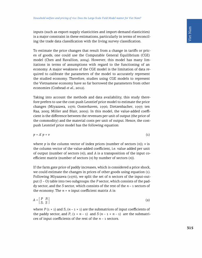
315
Vie
t N
am
Household welfare and pricing of rice: Does the Large-Scale Field Model matter for Viet Nam?
inputs (such as export-supply elasticities and import-demand elasticities) is a major constraint in these estimations, particularly in terms of reconcil-ing the trade data classification with the living survey classification.
To estimate the price changes that result from a change in tariffs or pric-es of goods, one could use the Computable General Equilibrium (CGE) model (Chen and Ravallion, 2004). However, this model has many lim-itations in terms of assumptions with regard to the functioning of an economy. A major weakness of the CGE model is the limitation of data re-quired to calibrate the parameters of the model to accurately represent the studied economy. Therefore, studies using CGE models to represent the Vietnamese economy have so far borrowed the parameters from other economies (Coxhead et al., 2012).
Taking into account the methods and data availability, this study there-fore prefers to use the cost-push Leontief price model to estimate the price changes (Miyazawa, 1976; Oosterhaven, 1996; Dietzenbacher, 1997; ten Raa, 2005; Miller and Blair, 2009). In this model, the value-added coeffi-cient is the difference between the revenues per unit of output (the price of the commodity) and the material costs per unit of output. Hence, the cost-push Leontief price model has the following equation:
p = A' p + v (1)
where p is the column vector of index prices (number of sectors (n)); v is the column vector of the value-added coefficient, i.e. value added per unit of output (number of sectors (n)), and A is a transposition of the input co-efficient matrix (number of sectors (n) by number of sectors (n)).
If the farm gate price of paddy increases, which is considered a price shock, we could estimate the changes in prices of other goods using equation (1). Following Miyazawa (1976), we split the set of n sectors of the input-out-put (I – O) table into two subgroups: the P sector, which consists of the pad-dy sector, and the S sector, which consists of the rest of the n – 1 sectors of the economy. The n × n input coefficient matrix A is:
A = PS1
PS
1 (2)
where P (1 × 1) and S1 (n – 1 × 1) are the submatrices of input coefficients of the paddy sector, and P1 (1 × n – 1) and S (n – 1 × n – 1) are the submatri-ces of input coefficients of the rest of the n – 1 sectors.

316
Trade policies, household welfare and poverty alleviation
Equation (1) could be re-written for the two subgroups as follows:
pp = P' pp + S'1 ps + vp
ps = P'1 pp + S' ps + vs (3)
where pp and ps are column vectors of index prices of the P sector’s prod-uct (which is paddy) and S sector’s products (which are the rest of the n – 1 products in the economy), respectively; vp and vs are P sector’s and S sec-tor’s column vectors of value-added coefficients, respectively; and P', S1', P1' and S' are transpositions of the matrices P, S1,P1, and S, respectively.
As we want to estimate the effects of paddy rice price changes on prices of other goods in the economy, in system (3), we take pp and vs as exogenous variables, whereas ps and vp are endogenous variables.
Under the cost-push effect, if the price of paddy rises from pp to (pp+∆pp), we could determine the price increase in other S sectors by solving the system as follows:
∆ps = ( I – S' ) –1 P1' ∆pp = T' P1' ∆pp = (P1 T)' ∆pp= T1' ∆pp (4)
Note that the price increase in other S sectors estimated under equation (4) could be viewed as a result of: (a) direct effects of change in the price of paddy, (b) second-order or indirect effects, and (c) paddy input in S sec-tors induced by internal propagation in S sector industries T1
= P1T = P1 (I – S) –1 (Miyazawa, 1976).
4.2 Estimating labour income effects
Wages are the key source of income for many households. They depend on the prices of goods, particularly given the fact that the Vietnamese la-bour market is segmented (M4P2, 2009). To estimate the elasticity of wag-es with respect to changes in prices, we can modify system (3) by splitting the value-added component of each sector into a wage component w (com-pensation of employees per unit of output) and a capital stock component r (rent paid to capital stock per unit of output):
pp = P' pp + S1' ps + wp + rp
ps = P1' pp + S' ps + ws + rs (5)
where vp = wp + rp
vs = ws + rs

317
Vie
t N
am
Household welfare and pricing of rice: Does the Large-Scale Field Model matter for Viet Nam?
If we take pp and vs as exogenous variables, whereas ps and vp are endog-enous variables, from system (5), the variation of vp could be seen as the change in wage in the P sector due to the change in price of the P sector’s product (Miyazawa, 1976). Under the cost-push effect, if the price of the P sector’s product increases from pp to ( pp + ∆pp ), under the assumption that capital stock coefficients rp and rs are constant in the short term and thus have not been affected by price changes, we obtain:
∆wp = { ( I – P' ) – S1' T' P1' } ∆pp (6)
The term ∆wp is the response of equilibrium wages in the P sector to the change in the prices of the P sector’s product.
The responses of the equilibrium wages to prices under equation (6) will differ across different sectors (industry wage premiums), but will be the same for household members working in the same sector, regardless of their labour skills.
4.3 Modelling welfare effects
Non-parametric density estimations and regressions are used here to study the distributional effects of rice price changes in relation to house-hold characteristics, particularly living standards and geographical loca-tions. The idea of non-parametric analysis was first introduced by Deaton (1989a) and then extensively used in various studies on welfare analy-sis (Deaton, 1989b; Budd, 1993; Benjamin and Deaton, 1993; Barrett and Dorosh, 1996; Sahn and Sarris, 1991). An extension of Deaton (1989a) con-siders the responses of the labour market because a change in the price of a good will affect labour demand and then the wage in the production sec-tor of this good.
For each household, the welfare impact could then be calculated as follows:
duh = ∑ ( Фph – Cp
h ) dpp + ∑ θjh εωp dpp (7)
where Фph is the share of household income from production of good p; Cp
h is the income share of household consumption spent on good p; θj
h is the share of wage income in total household income for member j; and εωp is the elasticity of wages earned with respect to the price of good p, estimat-ed in equation (6).
p p,j
318
Trade policies, household welfare and poverty alleviation
Note the following:
• One would expect that farming must be fairly competitive, so cost re-duction and productivity increases could lower the farm gate price of paddy. However, in the LSFM scheme, all paddy harvested in the large-scale fields will be purchased by exporters, as agreed upon by both par-ties under the contract. On the one hand, this ensures a secure source of high-quality rice for the exporter, on the other hand, farmers do not face competitive pressures (from other producers in the market), and hence do not need to reduce their paddy price.
• Therefore, in the policy simulation, we assume that there is no pass-through of productivity increases and production cost savings to the farm gate price of paddy sold by farmers who join the LSFM. Hence, the change in productivity and the lower cost of production only affect (pos-itively) the household income from paddy production in which the pro-ductivity gain (crop yield) leads to higher income, and the saving with regard to costs results in a lower cost of growing paddy.
• The increase in the price of paddy and the change in the price of oth-er goods (first step) affect both household incomes earned from produc-tion of these goods and household consumption of these goods. Slight increases in wages (second step) affect wage incomes of household members. Households’ exposure to price and wage changes depends on the structure of their income and the allocation of their expenditure
5 Data access and availability
For estimation of the price changes, this study uses the 2007 national I-O table published by the General Statistics Office of Viet Nam, which is the latest national benchmark I-O table based on a direct full survey released in 2010. Viet Nam’s 2007 I-O table classifies commodities and industries into 138 three-digit level commodities/industries.
For estimation of welfare effects, this study uses data from the 2010 Viet Nam Household Living Standards Survey, which was conducted by the GSO, with technical assistance from the United Nations Statistics Division, the World Bank, and Statistics Sweden. The surveys are representative at the national level.
In terms of sample design, the 2010 VHLSS is a classical three-stage strat-ified random survey covering ordinary households at the national level.

319
Vie
t N
am
Household welfare and pricing of rice: Does the Large-Scale Field Model matter for Viet Nam?
The sample size is quite large, with 45,000 households surveyed in the full sample each year. However, because a detailed questionnaire (including expenditures and other subject-specific modules) was applied to a random subsample of about 9,000 households, our policy simulations are based on the 9,000 households in the VHLSS that were selected for the full ques-tionnaire out of the 45,000 households surveyed. The 2010 VHLSS includes a number of modules providing information on demographics, education, employment, health, income, and labour supply. An expenditure module and extensive modules with information on farm activities related to agriculture, livestock, and aquaculture (including pro-duction, sale, inputs, and investment) are also included.
To reconcile the I-O table classification with the VHLSS sector classifica-tion, we aggregate the I-O table into 138 sectors and 81 sectors for estima-tions of household consumption/income effects and labour income effects, respectively.
Finally, we use data on monthly export prices of rice of Viet Nam and Thailand (in USD, current prices) as shown in Table A1 in the Annex. For the estimation of price transmission effects of the paddy price increase in the Mekong River Delta on other parts of the country (see Section 7.3), we use domestic prices of rice and farm gate prices of paddy (current prices) in the Mekong River Delta and the Red River Delta regions, which are avail-able from the Information Center for Agriculture and Rural Development (AgroInfor) for the period from January 2008 to the present.
6 Estimation of price change
The Vietnamese 2007 I-O table classifies commodities and industries into 138 three-digit level categories. This classification is almost perfectly con-cordant with the household consumption data and production income data. For labour income effects, we have to reconcile the I-O table with sectors of the household survey containing data on labour income. We thus aggre-gate the 138 sectors with the 81-sector classification of the household sur-vey’s labour income data.
Figure 5 presents our estimation of the top 20 price increases (out of 138) resulting from a 1 per cent increase in the farm gate paddy price, using equation (4). This vector of price changes for the 138-sector classification is used for the estimation of the consumption and production income ef-fects. The largest price increases are recorded for rice (0.8 per cent), flour
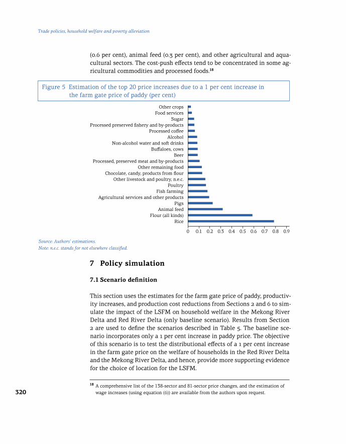
320
Trade policies, household welfare and poverty alleviation
(0.6 per cent), animal feed (0.3 per cent), and other agricultural and aqua-cultural sectors. The cost-push effects tend to be concentrated in some ag-ricultural commodities and processed foods.18
Figure 5 Estimation of the top 20 price increases due to a 1 per cent increase in the farm gate price of paddy (per cent)
Other cropsFood services
SugarProcessed preserved fishery and by-products
Processed coffeeAlcohol
Non-alcohol water and soft drinksBuffaloes, cows
BeerProcessed, preserved meat and by-products
Other remaining foodChocolate, candy, products from flour
Other livestock and poultry, n.e.c.Poultry
Fish farmingAgricultural services and other products
PigsAnimal feed
Flour (all kinds)Rice
0 0.1 0.2 0.3 0.4 0.5 0.6 0.7 0.8 0.9
Source: Authors’ estimations.Note: n.e.c. stands for not elsewhere classified.
18 A comprehensive list of the 138-sector and 81-sector price changes, and the estimation of wage increases (using equation (6)) are available from the authors upon request.
7 Policy simulation
7.1 Scenario definition
This section uses the estimates for the farm gate price of paddy, productiv-ity increases, and production cost reductions from Sections 2 and 6 to sim-ulate the impact of the LSFM on household welfare in the Mekong River Delta and Red River Delta (only baseline scenario). Results from Section 2 are used to define the scenarios described in Table 5. The baseline sce-nario incorporates only a 1 per cent increase in paddy price. The objective of this scenario is to test the distributional effects of a 1 per cent increase in the farm gate price on the welfare of households in the Red River Delta and the Mekong River Delta, and hence, provide more supporting evidence for the choice of location for the LSFM.

321
Vie
t N
am
Household welfare and pricing of rice: Does the Large-Scale Field Model matter for Viet Nam?
Source: Authors.
Scenario 1 is our short-term policy simulation, which incorporates not only the paddy price increase (9.9 per cent), but also the improvement in productivity (14 per cent) and the lower cost of paddy production (14.1 per cent).
It might be bold to assume that the increase in productivity following the LSFM would simply be equivalent to the difference in the observed pro-ductivity of large versus small farms. In scenarios 2 and 3, we therefore use productivity growth of only 5 and 10 per cent, respectively, to see how sensitive welfare is to changes in productivity growth.
It is important to note that the simulations assume that the farmers do not pass any cost reductions and productivity improvements on to the price of paddy. This assumption is based on the observed case of the LSFM run by the AGPPS (Dao et al., 2013), where farmers who join the LSFM are not in competition with other farmers in the market (see Section 4.3).
Table 5 Definition of scenarios
Location Parameters
Baseline scenario
Red River Delta and Mekong River Delta, rural areas
Paddy price increase by 1 per cent
Scenario 1 Mekong River Delta,rural areas
Paddy price increase by 9.9 per cent (owing to the direct farmers-exporters linkage)Production cost reduction by 14.1 per centProductivity increase by 14 per cent
Scenario 2 Mekong River Delta, rural areas
Paddy price increase by 9.9 per cent (owing to the direct farmers-exporters linkage)Production cost reduction by 14.1 per centProductivity increase by 5 per cent
Scenario 3 Mekong River Delta,rural areas
Paddy price increase by 9.9 per cent (owing to the direct farmers-exporters linkage)Production cost reduction by 14.1 per centProductivity increase by 10 per cent
Scenario 4 Mekong River Delta,rural areas
Paddy price increase by 9.9 per cent (owing to the direct farmers-exporters linkage)Further paddy price increase by 11.4 per cent (owing to the 11.4 per cent increase in the export price of rice)Production cost reduction by 14.1 per centProductivity increase by 14 per cent

322
Trade policies, household welfare and poverty alleviation
Scenario 4 is designed for a longer term: productivity grows by 14 per cent but, due to the upgrade of rice quality, exporters will have a stronger ca-pacity to bargain for an increase in the export price of rice. As discussed in Section 2, they could then agree to pass 59 per cent (equal to the share of paddy price in the export price of rice) of the increase in the export price of rice on to the producers. This would result in an 11.4 per cent increase of the farm gate price of paddy, in addition to the 9.9 per cent increase due to the direct farmers-exporters linkage.
7.2 Results
7.2.1 Baseline scenario simulation
Figure 6 shows total welfare effects. For rural households in the Red River Delta, estimations show that a 1 per cent increase in the farm gate price of paddy would not benefit the average household welfare across the entire income distribution. Losses decrease as household income increases, but the total effects on poor households are found to be significantly negative. The middle-income and rich households would be neither hurt nor better off. Due to the very small size of farms in the Red River Delta, the poorer households tend to be net consumers of rice – their gains from selling pad-dy are not large enough to offset the negative consumption effect, whereas the labour income effect is zero. Therefore, it is not surprising that, even though most of the poor rural households in the Red River Delta are rice farmers, faced with the paddy price increase, they are not better off.19
― Rural Viet Nam
― Rural RRD
Rural MRD
-.6
-.4
-.2
0
.2
4 6 8 10
Tota
l wel
fare
cha
nge
Ln (monthly income per capita)
Figure 6 Baseline scenario – Total welfare effects
Source: Authors’ calculations.
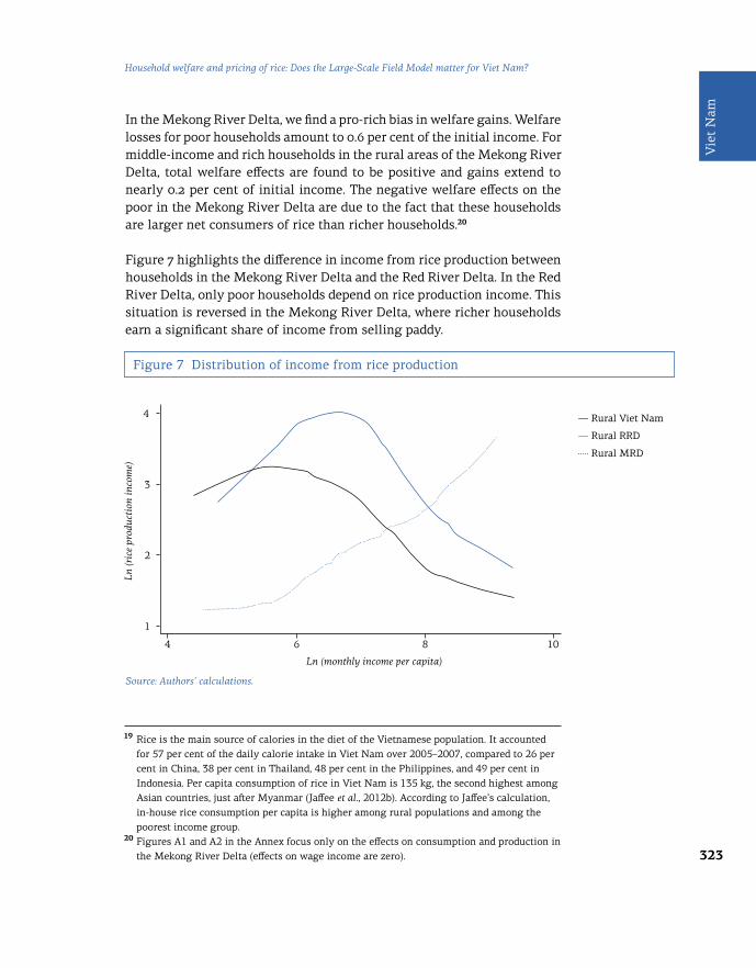
323
Vie
t N
am
Household welfare and pricing of rice: Does the Large-Scale Field Model matter for Viet Nam?
― Rural Viet Nam
― Rural RRD
Rural MRD
Figure 7 Distribution of income from rice production
Source: Authors’ calculations.
In the Mekong River Delta, we find a pro-rich bias in welfare gains. Welfare losses for poor households amount to 0.6 per cent of the initial income. For middle-income and rich households in the rural areas of the Mekong River Delta, total welfare effects are found to be positive and gains extend to nearly 0.2 per cent of initial income. The negative welfare effects on the poor in the Mekong River Delta are due to the fact that these households are larger net consumers of rice than richer households.20
Figure 7 highlights the difference in income from rice production between households in the Mekong River Delta and the Red River Delta. In the Red River Delta, only poor households depend on rice production income. This situation is reversed in the Mekong River Delta, where richer households earn a significant share of income from selling paddy.
1
2
3
4
4 6 8 10
Ln (r
ice
prod
ucti
on in
com
e)
19 Rice is the main source of calories in the diet of the Vietnamese population. It accounted for 57 per cent of the daily calorie intake in Viet Nam over 2005–2007, compared to 26 per cent in China, 38 per cent in Thailand, 48 per cent in the Philippines, and 49 per cent in Indonesia. Per capita consumption of rice in Viet Nam is 135 kg, the second highest among Asian countries, just after Myanmar (Jaffee et al., 2012b). According to Jaffee’s calculation, in-house rice consumption per capita is higher among rural populations and among the poorest income group. 20 Figures A1 and A2 in the Annex focus only on the effects on consumption and production in the Mekong River Delta (effects on wage income are zero).
Ln (monthly income per capita)

324
Trade policies, household welfare and poverty alleviation
Figure 8 shows rice income by farm size. In the Red River Delta, income from rice production does not merely depend on farm size or the level of household income. As discussed in Section 2.2, larger fragmentation in the Red River Delta is a constraint for farmers to achieve economies of scale. In the Mekong River Delta, however, productivity gains would be higher and income earnings from rice production hence greater for larg-er farms and higher levels of household income (poor households usually have no land for cultivation and gain income by working for other rich-er households).21
21 As explained above, agricultural land in Viet Nam belongs to the state and is only for lease for a 20-year period (according to the Land Law). Unlike farmers in the Red River Delta, to whom agricultural land was redistributed according to their household size during 1953– 1957, farm size in the Mekong River Delta is a result of the historical development of this region and does not depend on the size of households.
Figure 8 Rice income by farm size
― Red River Delta
― Mekong River Delta
8
8
6
6
4
4
2
2
Ln (r
ice
prod
ucti
on in
com
e pe
r ca
pita
)
4
4
4
4
6
6
6
6
8
8
8
8
10
10
10
10
Ln (income per capita)Source: Authors’ calculations.
In conclusion, our baseline scenario suggests that farmers in the Red River Delta who work on small farms are net consumers of rice and hence might not benefit from the paddy price increase under the LSFM. However, farm-ers in the Mekong River Delta are likely to be potential members of the LSFM policy target group. Because larger gains would be captured by rich-er households, households with a farm size of 2 ha or above would benefit more from participating in the LSFM.
Under 0.2 ha
0.5 to 2 ha 2 ha and above
0.2 to 0.5 ha
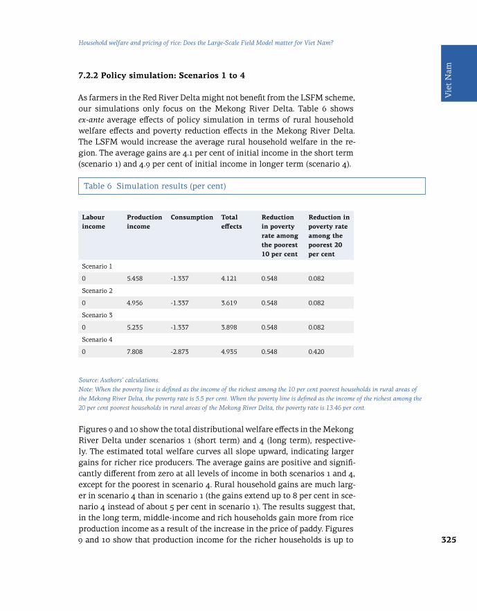
325
Vie
t N
am
Household welfare and pricing of rice: Does the Large-Scale Field Model matter for Viet Nam?
Table 6 Simulation results (per cent)
Source: Authors’ calculations.Note: When the poverty line is defined as the income of the richest among the 10 per cent poorest households in rural areas of the Mekong River Delta, the poverty rate is 5.5 per cent. When the poverty line is defined as the income of the richest among the 20 per cent poorest households in rural areas of the Mekong River Delta, the poverty rate is 13.46 per cent.
7.2.2 Policy simulation: Scenarios 1 to 4
As farmers in the Red River Delta might not benefit from the LSFM scheme, our simulations only focus on the Mekong River Delta. Table 6 shows ex-ante average effects of policy simulation in terms of rural household welfare effects and poverty reduction effects in the Mekong River Delta. The LSFM would increase the average rural household welfare in the re-gion. The average gains are 4.1 per cent of initial income in the short term (scenario 1) and 4.9 per cent of initial income in longer term (scenario 4).
Labour income
Production income
Consumption Total effects
Reduction in poverty rate among the poorest 10 per cent
Reduction in poverty rate among the poorest 20 per cent
Scenario 1
0 5.458 -1.337 4.121 0.548 0.082
Scenario 2
0 4.956 -1.337 3.619 0.548 0.082
Scenario 3
0 5.235 -1.337 3.898 0.548 0.082
Scenario 4
0 7.808 -2.873 4.935 0.548 0.420
Figures 9 and 10 show the total distributional welfare effects in the Mekong River Delta under scenarios 1 (short term) and 4 (long term), respective-ly. The estimated total welfare curves all slope upward, indicating larger gains for richer rice producers. The average gains are positive and signifi-cantly different from zero at all levels of income in both scenarios 1 and 4, except for the poorest in scenario 4. Rural household gains are much larg-er in scenario 4 than in scenario 1 (the gains extend up to 8 per cent in sce-nario 4 instead of about 5 per cent in scenario 1). The results suggest that, in the long term, middle-income and rich households gain more from rice production income as a result of the increase in the price of paddy. Figures 9 and 10 show that production income for the richer households is up to

326
Trade policies, household welfare and poverty alleviation
8 per cent in scenario 4 compared to 4 per cent in scenario 1. Expenditure on rice also increases for all households. However, the poorest households are the most adversely affected because their rice expenditure increases by 8 per cent in scenario 1 and by 16 per cent in scenario 4. This is more than the increase in these households' income from rice production, making the total welfare effect of the rice price increase negative for them.
Policy simulation results presented in Table 6 also show poverty reduction effects in the Mekong River Delta. Poverty rate estimations use per capita income from the 2010 VHLSS. In both short-term and longer-term scenar-ios, the reductions in the poverty rate among the poorest 10 per cent are the same, namely 0.548 per cent. This is because the poorest 10 per cent in the Mekong River Delta do not produce rice at all, as they do not have ac-cess to agricultural land, as explained above. Therefore, different scenari-os only affect them as net consumers.
With regard to poverty reduction among the poorest 20 per cent, because we include one richer decile of households among the poorest rural de-ciles, an additional 11.4 per cent increase in the paddy price under scenario 4 does move some of the poor across the poverty line. As a result, attaina-ble poverty reduction is higher in the longer term (0.420 per cent versus 0.082 per cent).
In scenarios 2 and 3, we try to see how sensitive our simulations are to the assumed productivity increase. Results presented in Table 6 show that to-tal welfare effects decrease (due to the lower level of productivity gains) but that the impact on poverty reduction remains unchanged in both pov-erty rate definitions (10 per cent and 20 per cent, respectively).

327
Vie
t N
am
Household welfare and pricing of rice: Does the Large-Scale Field Model matter for Viet Nam?
Figure 9 Scenario 1 – Total welfare effects
Figure 10 Scenario 4 – Total welfare effects
-8
-16
-8
-12
-4
-4
0
0
8
8
4
4
12
16
12
Tota
l wel
fare
cha
nge
Tota
l wel
fare
cha
nge
4
4
5
5
6
6
7
7
8
8
9
9
10
10
Ln (monthly income per capita)
Ln (monthly income per capita)
Expenditure change
― Wage income change
― Production income change
Total welfare change
Expenditure change
― Wage income change
― Production income change
Total welfare change
Source: Authors’ calculations.
Source: Authors’ calculations.
7.3 Discussion of potential side effects of the Large-Scale Field Model
Although it is not quantitatively shown in our simulation results, the joint effects of the LSFM would not only increase rural household welfare in the Mekong River Delta but also increase the volume and value of rice exports (through productivity improvements and higher

328
Trade policies, household welfare and poverty alleviation
export prices). Therefore, some side effects of the LSFM might be of con-cern to policymakers. These effects may relate to: (a) national food securi-ty – whether or not it could be compromised if and when the LSFM results in an increase in the value and the volume of rice exports, and (b) wheth-er there would be price transmission effects of the paddy price increase in the Mekong River Delta on other parts of the country.
Regarding the first potential side effect, Jaffee et al. (2012b) show that, in 2030, the expected output would be far in excess of national food security needs even under the worst-case scenario of a reduction of paddy land to 3 million ha (from 4 million ha), given the current low level of productivity (5.8 metric tons per ha) and assuming that the domestic rice consumption remains at 120 kg per capita per year and there is no change in post-har-vest losses (10 per cent at the farm level).
Regarding the second side effect, because the paddy price change would directly affect the domestic price of rice, we could assume that the law of one price holds. This implies that any change in the farm gate price of pad-dy would be fully transmitted to the domestic price of rice in the Mekong River Delta. Therefore, we could apply a simple framework to examine the price transmission effects of the paddy price increase in the Mekong River Delta. The domestic price of rice in time t in the Red River Delta is a func-tion of domestic prices of rice in the Mekong River Delta:
ln ptMRD = β0 + β1 ln pt
RRD + ε (8)
Econometric estimations use panel data on weekly domestic paddy pric-es from 1 January 2008 to 20 August 2013. The results are shown in Table A2 in the Annex. We use dummies for monthly fixed effects. The estimat-ed pass-through elasticity is close to zero and statistically significant. This implies no price transmission between the Mekong River Delta and the Red River Delta. This result confirms that an increase in the farm gate price of paddy following the LSFM would not affect the domestic price of rice in the rest of Viet Nam.
If the LSFM were applied on a region-wide scale, it is likely that additional exporters would join the scheme. As the LSFM leads to productivity gains and cost reductions, one would expect the domestic price of paddy to de-crease over the longer run (at least partially in the Mekong River Delta re-gion), due to greater market competition among farmers.

329
Vie
t N
am
Household welfare and pricing of rice: Does the Large-Scale Field Model matter for Viet Nam?
8 Conclusions
This study has examined the potential impact of the adoption of the Large-Scale Field Model on household welfare and poverty reduction in the Mekong River Delta.
The study has first found that an increase of 1 per cent in the price of paddy would benefit households in the Mekong River Delta but not households in the Red River Delta. The larger fragmentation of land in the Red River Delta makes it difficult to implement the LSFM. We therefore suggest that farmers from the Mekong River Delta be given priority for the application of the LSFM. Within this policy target group, households with a farm size of 2 ha or above would likely benefit more from participating in the LSFM.
The estimation of ex-ante effects shows that the LSFM would improve av-erage rural household welfare by 4.1 per cent in the short term and by 4.9 per cent in the longer term. In all scenarios, the LSFM would result in pov-erty reduction in the Mekong River Delta. The effective poverty reduction would be higher in the longer term, when exporters could bridge the gap between export prices of Viet Nam and Thailand.
As the LSFM idea has been met with considerable interest by the gov-ernment of Viet Nam, as well as by local authorities in provinces in the Mekong River Delta, we suggest that to attain the government’s objec-tive of a minimum rate of return of 30 per cent for rice farmers, the LSFM might be a better policy option than setting price floors for export prices and farm gate prices of paddy.
As discussed above, the combined effects of the LSFM would not only im-prove household welfare in the region but also foster Vietnamese rice ex-ports. As state-owned exporters may have fewer incentives to implement the changes proposed by the LSFM scheme, private exporters would like-ly be better candidates to lead the implementation of this policy. The rice export quota granted to SOEs could be a bottleneck, however, because the implementation of the LSFM requires that some level of competition be established among Vietnamese rice exporters.
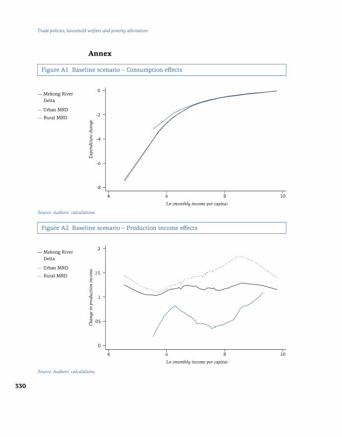
330
Trade policies, household welfare and poverty alleviation
Annex
Figure A1 Baseline scenario – Consumption effects
Figure A2 Baseline scenario – Production income effects
-8
0
-6
.05
-4
.1
0
.2
-2
.15
Expe
ndit
ure
chan
geC
hang
e in
pro
duct
ion
inco
me
4
4
6
6
8
8
10
10
Ln (monthly income per capita)
Ln (monthly income per capita)
― Mekong River Delta
― Urban MRD
Rural MRD
― Mekong River Delta
― Urban MRD
Rural MRD
Source: Authors’ calculations.
Source: Authors’ calculations.

331
Vie
t N
am
Household welfare and pricing of rice: Does the Large-Scale Field Model matter for Viet Nam?
Figure A3 Viet Nam regional map
Source: General Statistics Office of Viet Nam.Note: The eight socio-ecological zones recognized by the GSO are: (1) Red River Delta, (2) North-East, (3) North-West, (4) North Central Coast, (5) South Central Coast, (6) Central Highlands, (7) South-East, and (8) Mekong River Delta.
Thailand
China
Lao People's Democratic Republic
Yunnan Province
Guangxi Province
Cambodia
Viet Nam
8
7
6
N
5
4
3
2
1
Hanoi
■ ■
■
■
Haiphong
Hue
Ho Chi Minh City
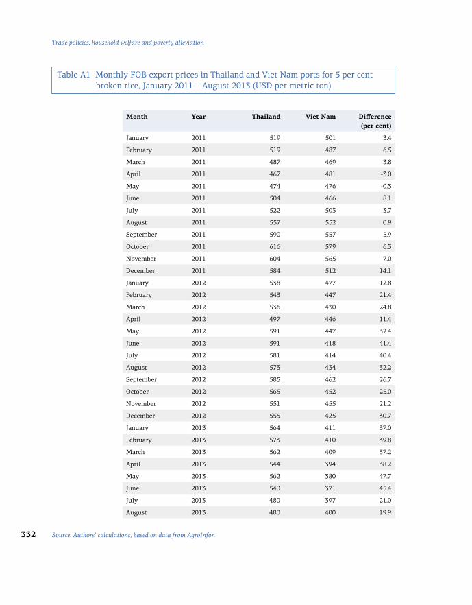
332
Trade policies, household welfare and poverty alleviation
Month Year Thailand Viet Nam Difference (per cent)
January 2011 519 501 3.4
February 2011 519 487 6.5
March 2011 487 469 3.8
April 2011 467 481 -3.0
May 2011 474 476 -0.3
June 2011 504 466 8.1
July 2011 522 503 3.7
August 2011 557 552 0.9
September 2011 590 557 5.9
October 2011 616 579 6.3
November 2011 604 565 7.0
December 2011 584 512 14.1
January 2012 538 477 12.8
February 2012 543 447 21.4
March 2012 536 430 24.8
April 2012 497 446 11.4
May 2012 591 447 32.4
June 2012 591 418 41.4
July 2012 581 414 40.4
August 2012 573 434 32.2
September 2012 585 462 26.7
October 2012 565 452 25.0
November 2012 551 455 21.2
December 2012 555 425 30.7
January 2013 564 411 37.0
February 2013 573 410 39.8
March 2013 562 409 37.2
April 2013 544 394 38.2
May 2013 562 380 47.7
June 2013 540 371 45.4
July 2013 480 397 21.0
August 2013 480 400 19.9
Source: Authors’ calculations, based on data from AgroInfor.
Table A1 Monthly FOB export prices in Thailand and Viet Nam ports for 5 per cent broken rice, January 2011 – August 2013 (USD per metric ton)
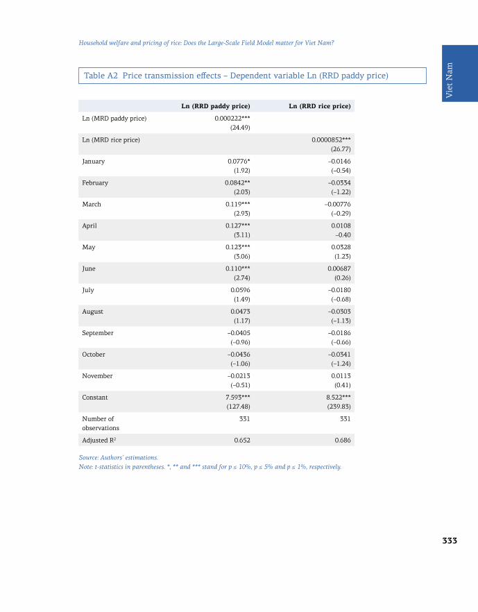
333
Vie
t N
am
Household welfare and pricing of rice: Does the Large-Scale Field Model matter for Viet Nam?
Table A2 Price transmission effects – Dependent variable Ln (RRD paddy price)
Ln (RRD paddy price) Ln (RRD rice price)
Ln (MRD paddy price) 0.000222***(24.49)
Ln (MRD rice price) 0.0000852***(26.77)
January 0.0776*(1.92)
–0.0146(–0.54)
February 0.0842**(2.03)
–0.0334(–1.22)
March 0.119***(2.93)
–0.00776(–0.29)
April 0.127***(3.11)
0.0108–0.40
May 0.123***(3.06)
0.0328(1.23)
June 0.110***(2.74)
0.00687(0.26)
July 0.0596(1.49)
–0.0180(–0.68)
August 0.0473(1.17)
–0.0303(–1.13)
September –0.0405(–0.96)
–0.0186(–0.66)
October –0.0436(–1.06)
–0.0341(–1.24)
November –0.0213(–0.51)
0.0113(0.41)
Constant 7.593***(127.48)
8.522***(239.83)
Number of observations
331 331
Adjusted R2 0.652 0.686
Source: Authors’ estimations.Note: t-statistics in parentheses. *, ** and *** stand for p ≤ 10%, p ≤ 5% and p ≤ 1%, respectively.

334
Trade policies, household welfare and poverty alleviation
References
AgroInfor (2009). “Vietnam Annual Rice Market Report 2008.” Information Center for Agriculture and Rural Development. Institute of Policies and Strategies for Agriculture and Rural Development, Hanoi.
Balat, J., Brambilla, I. and Porto, G. (2009). “Realizing the Gains from Trade: Export Crops, Marketing Costs, and Poverty.” Journal of International Economics, 78 (1): 21–31.
Barrett, C.B. and Dorosh, P.A. (1996). “Farmers’ Welfare and Changing Food Prices: Nonparametric Evidence from Rice in Madagascar.” American Journal of Agricultural Economics, 78 (3): 656–669.
Benjamin, D. and Brandt, L. (2002). “Agriculture and Income Distribution in Rural Vietnam under Economic Reforms: A Tale of Two Regions.” William Davidson Institute Working Paper 519, University of Michigan.
Benjamin, D. and Deaton, A. (1993). “Household Welfare and the Pricing of Cocoa and Coffee in Côte d'Ivoire: Lessons from the Living Standards Surveys.” World Bank Economic Review, 7 (3): 293–318.
Boycko, M., Shleifer, A. and Vishny, R.W. (1996). “A Theory of Privatisation.” The Economic Journal, 106 (435): 309–319.
Budd, J. (1993). “Changing Food Prices and Rural Welfare: A Nonparametric Examination of the Côte d’Ivoire.” Economic Development and Cultural Change, 4 (3): 587–603.
Chen, S. and Ravallion, M. (2004). “Welfare Impacts of China’s Accession to the World Trade Organization.” World Bank Economic Review, 18 (1): 29–57.
Chi-Chung, C., Bruce, A.M., Ching-Cheng, C. and Shih-Hsun, H. (2002). “Spatial Equilibrium Modeling with Imperfectly Competitive Markets: An Application to Rice Trade.” Presentation at the American Agricultural Economics Association’s 2002 Annual Meeting, Long Beach CA, 28–31 July.
Coxhead, I., Linh, V.H. and Tam, L.D. (2012). “Global Market Shocks and Poverty in Vietnam: The Case of Rice.” DEPOCEN Working Paper No. 2012/32. Development and Policies Research Center, Hanoi.
Dao, M.H.T., Nguyen, A.V. and Vo, L.M.T. (2013). “Linkages in Rice Production and Consumption in Vietnam.” VIE Report. Vietnam Institute of Economics, Hanoi.
Deaton, A. (1989a). “Rice Prices and Income Distribution in Thailand: A Non-Parametric Analysis.” Economic Journal, 99 (395): 1–37.
Deaton, A. (1989b). “Household Survey Data and Pricing Policies in Developing Countries.” World Bank Economic Review, 3 (2): 183–210.
Dietzenbacher, E. (1997). “In Vindication of the Ghosh Model: A Reinterpretation as a Price Model.” Journal of Regional Science, 37 (4): 629–651.
Francois, J.F. and Hall, H.K. (2009). “Global Simulation Analysis of Industry-Level Trade Policy: The GSIM Model.” IIDE Discussion Paper No. 20090803. Institute for International and Development Economics, Rotterdam.
GSO (various years). Statistical Yearbooks of 2006–2011. General Statistics Office, Hanoi.
IRRI (2006). Paddy Drying Systems [online]. International Rice Research Institute, Manila. Available at: http://www.knowledgebank.irri.org/training/fact-sheets/postharvest-management/drying-fact-sheet-category/paddy-drying-systems-fact-sheet.

335
Vie
t N
am
Household welfare and pricing of rice: Does the Large-Scale Field Model matter for Viet Nam?
Jaffee, S., Nguyen, S.V., Le, D.C. and Vo, L.T.T. (2012a). “From Rice Bowl to Rural Development: Challenges and Opportunities Facing Vietnam’s Mekong Delta Region.” In: World Bank Ed. Vietnam Rice, Farmers and Rural Development: From Successful Growth to Sustainable Prosperity. World Bank, Washington DC.
Jaffee, S., Nguyen, T.A.D., Nguyen, Q.N., Dao, A.T., Nguyen, D.T., Nguyen, M.N., Nguyen, V. and Nguyen, P.A. (2012b). “Moving the Goal Posts: Vietnam’s Evolving Rice Balance and Other Food Security Considerations.” In: World Bank Ed. Vietnam Rice, Farmers and Rural Development: From Successful Growth to Sustainable Prosperity. World Bank, Washington DC.
Le, H.M. Ed. (2007). The General History of Vietnam. Vol. 3. Hanoi: Education Publishing House.
M4P2 (2009). “Improving the Relevance of the TVET System to the Needs of the Private Sector.” Making Markets Work Better for the Poor II, M4P2 Project. Asian Development Bank and United Kingdom Department for International Development.
Markussen, T., Tarp, F., Do, T.H. and Nguyen, T.A.D. (2012). “Inter- and Intra-farm Land Fragmentation in Vietnam.” CIEM Policy Brief 06. Central Institute for Economic Management, Hanoi.
Miller, R.E. and Blair, P.D. (2009). Input-Output Analysis: Foundations and Extensions. Second Edition. Cambridge: Cambridge University Press.
Minot, N. and Goletti, F. (1998). “Export Liberalization and Household Welfare: The Case of Rice in Vietnam.” American Journal of Agricultural Economics, 80 (4): 738–749.
Minot, N. and Goletti, F. (2000). “Rice Market Liberalization and Poverty in Vietnam.” Research Report 114. International Food Research Institute, Washington DC.
Miyazawa, K. (1976). Input-Output Analysis and the Structure of Income Distribution. Lecture Notes in Economics and Mathematical Systems. No. 116. Berlin: Springer Verlag.
Nicita, A., Hoekman, B. and Olarreaga, M. (2005). “Estimating the Effect of Global Trade Reforms.” In: Hoekman, B. and Olarreaga, M. Ed. Doha and Poverty in Low Income Countries. New Haven CT: Yale University Press.
Oosterhaven, J. (1996). “Leontief versus Ghoshian Price and Quantity Models.” Southern Economic Journal, 62 (3): 750–759.
Pham, N.Q., Bui, T. and Nguyen, T.D. (2007). “Economic Performance of Vietnam, 1976–2000: New Evidence from Input-Output Model.” DEPOCEN Working Paper Series No. 2007/13. Development and Policies Research Center, Hanoi.
Sahn, D.E. and Sarris, A. (1991). “Structural Adjustment and the Welfare of Rural Smallholders: A Comparative Analysis from Sub-Saharan Africa. “World Bank Economic Review, 5 (2): 259–289.
ten Raa, T. (2005). The Economics of Input-Output Analysis. Cambridge: Cambridge University Press.
Tran, T.C., Do, H.L. and Le, M.N. (2013). Who Has Benefited From High Rice Prices in Vietnam? Oxfam International, Hanoi.
VFA (2006). “Important Export Growth during 1989-2005 [online].” Vietnam Food Association, Hanoi. Available at:http://www.vietfood.org.vn/vn/newwindow.aspx?n=907
Vo, L.T.T. and Nguyen, S.P. (2011). “Part 1: Analysis of Rice Value Chains in the Red River Delta Region.” Scientific Journal, 19a: 96–108.
