trade policy and poverty reduction in...

Trade Policy and Poverty Reduction in Brazil

Glenn W. Harrison, Thomas F. Rutherford, David G. Tarr,and Angelo Gurgel

A multiregion computable general equilibrium model is used to evaluate the regional,multilateral, and unilateral trade policy options of Mercosur from the perspective ofthe welfare of all potential partners in several proposed agreements. The focus forBrazil is on poverty impacts. The results show that the poorest households in Brazilexperience gains of 1.5–5.5 percent of their consumption, which are about three to fourtimes the average gains for Brazil. Protection in Brazil favors capital-intensive manu-facturing relative to unskilled labor-intensive agriculture and manufacturing. So tradeliberalization raises the return to unskilled labor relative to capital and disproportio-nately helps the poor.

Brazil has several trade policy options. This study evaluates those options fromthe perspective of the welfare of all potential partners in several proposed tradeagreements, looking particularly at the impacts on poor people to determinewhich trade policy contributes most to poverty reduction in Brazil. The objec-tive is to determine whether there is a tradeoff between aggregate welfare gainsto Brazil from trade liberalization and the welfare gains to the poor. The articleconcludes that there is no tradeoff and explains why.

As part of the Mercosur customs union with Argentina, Paraguay, andUruguay, Brazil is engaged in negotiations to implement the Free Trade Agree-ment of the Americas (FTAA). Mercosur is also negotiating a potential free trade

Glenn W. Harrison is professor of economics at the University of Central Florida; his e-mail address is

[email protected] is professor of economics at theUniversity ofColorado;

his e-mail address is [email protected]. David G. Tarr is lead economist at the World Bank; his

e-mail address is [email protected]. Angelo Gurgel is professor of economics at the Universidade de

Sao Paulo in Brazil; his e-mail address is [email protected]. The authors thank seminar

participants at the Institute for Applied Economic Research in Brasilia, the Brazilian Development

Bank in Rio de Janeiro, and the GTAP conference in Taiwan, China; agencies of the government of Brazil

and Brazilian research institutes; and Brazilian scholars including Francisco Ferreira, Renato Flores,

Claudio Fritschak, Marcelo Neri, Armando Castelar Pinheiro, Lia Valls Pereira, Octavio Tourinho,

and William Tyler. They also thank Mary Burfisher, Mauricio Carrizosa, Carsten Fink, Paul Gibson,

Bernard Hoekman, Maria Kasilag, Peter Lanjouw, Daniel Lederman, Aaditya Mattoo, Johan Mistian,

Sherman Robinson, Maurice Schiff, Claudia Paz Sepulveda, Mark Thomas, Vinod Thomas, Alberto

Valdes, Dominique van der Mensbrugge, and Joachim von Amsberg for help and comments. The authors

gratefully acknowledge research support under the Bank-Netherlands Partnership Program to examine

the impact of trade policy on poverty.

THE WORLD BANK ECONOMIC REVIEW, VOL. 18, NO. 3,

� The International Bank for Reconstruction and Development / THE WORLD BANK 2004; all rights reserved.

doi:10.1093/wber/lhh043 18:289–317

289

Pub

lic D

iscl

osur

e A

utho

rized

Pub

lic D

iscl

osur

e A

utho

rized

Pub

lic D

iscl

osur

e A

utho

rized

Pub

lic D

iscl

osur

e A

utho

rized

Pub

lic D

iscl

osur

e A

utho

rized

Pub

lic D

iscl

osur

e A

utho

rized

Pub

lic D

iscl

osur

e A

utho

rized

Pub

lic D

iscl

osur

e A

utho

rized

wb451538

Typewritten Text

77479

agreement with the European Union, along with less notable regional arrange-ments. In addition, Brazil has supported further multilateral negotiations withinthe World Trade Organization (WTO 2000).

Brazil is concerned that these regional integration initiatives will providemuch less market access than agreements that do not constrain the exports ofpartner countries. Notably, significantly improved access to EU agriculturalmarkets will be very difficult to achieve for the usual EU internal politicalreasons. As a major agricultural exporter, Brazil believes that the WTO is thebest negotiating forum for obtaining freer access to agricultural markets. More-over, antidumping and stringent rules of origin may limit access to the marketsof the main industrial country partners in these regional agreements, especiallythe Free Trade Agreement of the Americas (FTAA).

Extending the analysis of Harrison and others (2002) on Chile, this studyevaluates the value of trade policy options to Brazil if the key industrial countrypartner in these regional agreements denies access to specific products. For theEU, that means exclusion of preferred access to Mercosur exporters in the mosthighly protected agricultural products. For the FTAA, that means denial to Brazilof access to the most highly protected products in the United States because ofantidumping measures or restrictive rules of origin.

A major policy concern is the link between trade policy changes and poverty inBrazil. Although interest in the topic has increased dramatically in recent years,using general equilibrium modeling with multiple households to examine equityissues dates to pioneering studies by Adelman and Robinson (1978) and Piggot andWhalley (1985). This has typically been done by aggregating households from ahousehold survey into 5–40 households.1 Recently modelers have focused attentionon the impact of trade policy on poverty, and Harrison and others (2003a) haveshowed that a concern with equity is not equivalent to a concern with poverty.2

A second approach is to take price changes from a representative consumergeneral equilibrium model and feed these into a micro-simulation model ofhousehold behavior, such as in Chen and Ravallion (2003) and Bussolo andLay (2003). This approach allows examination of the diversity of impacts acrosshouseholds: Even if the aggregated poor households gain, many individual poorhouseholds could lose. But the approach ignores feedback effects of the quantitychanges on the equilibrium outcome in the general equilibrium model and doesnot reconcile inconsistent information on household income from the nationalaccounts and the household surveys.3

The analysis here is in the tradition of the first approach. The modelincorporates 20 types of Brazilian households: 10 rural and 10 urban, with

1. For recent applications see the papers for the conference on Poverty and the International

Economy (available online at www.worldbank.org/trade).

2. The trade policy change they evaluated resulted in an increase in aggregate real income and greater

equity as measured by the Gini coefficient, but the poorest households were worse off.

3. See Cockburn (2001) for an attempt to combine the two approaches.

290 THE WORLD BANK ECONOMIC REV I EW, VOL . 18 , NO . 3

households further classified by income level. The results show clear and cruciallinks among trade policy changes, factor intensities at the industry level,economy-wide factor returns, and poverty—the links suggested by theHekscher-Ohlin and Stolper-Samuelson models. But only because of the atten-tion to detail in the empirical estimation of factor shares are results obtainedthat can be sensibly used to analyze the poverty dimension of trade policychanges. The results also show the importance of agricultural liberalizationfor the poor.

The aggregate policy results show that both the FTAA and the EU–Mercosurarrangements are net trade creating for member countries, but excluded coun-tries almost always lose. But multilateral trade liberalization (a 50 percent cutin tariffs and export subsidies) results in estimated gains to the world that aremore than four times greater than the returns for either the FTAA or the EU–Mercosur agreement, demonstrating the continuing importance of multilateralnegotiations.

A fully implemented agreement with the European Union is about 1.5 timesmore valuable to Brazil than the FTAA because of access to highly protected EUagricultural markets. But if agriculture is excluded from the agreement, itbecomes of very little value to Brazil. Application of antidumping and restrictiverules of origin by the United States against Brazil on the most protected productsin the U.S. market similarly reduces the value of the FTAA to Brazil. Nonetheless,the FTAA still has significant value to Brazil because other markets in theAmericas and the less protected sectors in the United States are assumed toremain open to Brazilian exporters.

Most of the evaluated trade policy options result in a progressive distributionof the gains, so that the poorest households experience the greatest percentageincrease in their incomes. Although Brazil undertook substantial trade liberal-ization in the 1990s, vestiges of its import-substitution industrialization strategyof the 1960s remain. Trade policy reforms in Brazil tend to shift resources fromcapital-intensive manufacturing to unskilled labor-intensive agriculture and lesscapital-intensive manufacturing, increasing the wages of unskilled labor relativeto returns to capital and skilled labor. The percentage increase in the incomes ofthe eight poorest types of households is several times greater than the averagepercentage increase for the economy as a whole.4

Previous work has shown that multilateral agricultural trade liberalizationwill lead to aggregate gains for agricultural exporting nations. The results heresuggest that agricultural trade liberalization, whether multilateral or in a regio-nal arrangement with the European Union, is particularly important for therealization of poverty reduction benefits for agricultural exporters, such asBrazil.

4. These results are consistent with two other analyses of the impact of trade liberalization on the

poor in Brazil: Barros and others (2000) and World Bank (2001).

Harrison and others 291

I . A MULTIREGIONAL TRADE MODEL

A comparative static, constant returns to scale, multiregional, and multisectoralquantitative model is developed to evaluate the impact of trade policy onpoverty in Brazil. The model is relatively detailed in the Americas, with 13countries or regions from that area (table 1). Also included are the EuropeanUnion 15, Japan, and a residual rest of the world. Of the Mercosur members,Brazil, Argentina, and Uruguay are represented explicitly in the model, whereasParaguay is represented as part of the rest of South America. The generalspecification of this model follows the earlier multiregional model of the effectsof the Uruguay Round in Harrison and others (1997c) and even more closelytheir model of trade policy options for Chile (Harrison and others 2002).5

Because most of the documentation of the data and model and additionalsimulations are available in Harrison and others (2003b), only the main features

TABLE 1. List of Commodities, Regions, and Factors of Production Usedin the Model

Commodities Regions Factors

PDR Paddy rice BRA Brazil CapitalGRO Cereal grains ARG Argentina Unskilled laborOSD Oilseeds URY Uruguay LandAGR Other agriculture CHL Chile Natural resourcesOCR Other crops COL Colombia Skilled laborCMT Bovine meat products PER PeruOMT Other meat products VEN VenezuelaMIL Dairy products XAP Rest of Andean pactPCR Processed rice MEX MexicoSGR Sugar XCM Central America

and CaribbeanOFD Other food products XSM Rest of South AmericaENR Energy and mining CAN CanadaTEX Textiles USA United StatesWAP Wearing apparel E_U European Union 15LEA Leather products JPN JapanLUM Wood products ROW Rest of worldMAN Other manufacturingI_S Iron and steelFMP Other metal productsMVH Motor vehicles and partsSER ServicesCGD Savings goodDWE Dwellings

5. Harrison and others (1997c, 2002). The model is formulated using the GAMS-MPSGE software

developed by Rutherford (1999) and solved using the PATH algorithm of Ferris and Munson (2000). See

de Melo and Tarr (1992) for an exposition of the general form of the within-country equations of the

model.


are summarized here.6 Production uses intermediate inputs and primary factors(labor, capital, and land) that are mobile across sectors within a region butimmobile internationally. The amount of capital and labor available to anyeconomy is fixed. Output is differentiated between domestic output andexports, but exports are not differentiated by destination country. Except forBrazil, each region has a single representative consumer who maximizes utility,as well as a single government agent. Demand is characterized by a nestedArmington structure for each of the 22 sectors (see table 1). The Armingtonaggregate good is a constant elasticity of substitution (CES) composite of domes-tic production and aggregate imports, and aggregate imports are a CES aggregateof imports from different regions of origin. This structure allows multistagebudgeting. So government revenue remains unchanged in any counterfactualscenario, a tax is imposed to compensate for lost tariff revenue. Each countryhas a balance of trade constraint, so any change in the value of imports ismatched by an equal value change in exports. The model is ‘‘real,’’ in the sensethat it contains no financial assets. Thus there is only a ‘‘real’’ exchange rate,defined as the price of a country’s tradable goods relative to the price of itsnontradable goods.

The model does not incorporate increasing returns to scale or endogenousproductivity effects of trade policy, despite a number of studies by Brazilianresearchers identifying a correlation between the opening of Brazil to externaltrade in the early 1990s and an increase in productivity in Brazilian manufac-turing (Muendler 2001 found a causal relationship). A model that incorporatesboth of these, such as that developed in Rutherford and Tarr (2002), would beexpected to produce much larger gains than this constant returns to scale model,with a resulting further reduction in Brazilian poverty. But because the produc-tivity advances are not likely to be concentrated in the labor-intensive sectors,the relative share of the gains at the household level for the poor may be lessprogressive than that found here.7

Brazilian Households

The most important new feature in this model is the extension to multiplehouseholds in Brazil: 10 rural households and 10 urban households, distin-guished by income levels (as defined in table 2). The structure of demand foreach household is a nested Armington structure, based on CES demand functions,similar to representative households in other regions.

6. These appendixes present details of the model specification, tables with low elasticity results and

detailed sectoral results for Brazil, procedures for updating the input-output tables and estimating factor

intensities, calculation of the tariff rates in Mercosur, systematic sensitivity analysis, steps for incorpor-

ating the household survey information, and some additional references.

7. Most of the trade policy options were also evaluated in separate simulations in a comparative

steady-state model. Because the rental rate on capital falls in most of the scenarios, the new equilibrium

capital stock does not rise, and the estimated welfare gains to the economy also do not rise.


TABLE2.Household

Types

andCharacteristics

Rural

Households

Mean

per

Capita

Incomea

Mean

Household

Incomea

%of

Sample

Representative

no.

Individualsb

(millions)

No.

Individuals

inSurvey

Urban

Households

Mean

per

Capital

Income

Mean

Household

Incomea

%of

Sample

Representative

no.

Individualsb

(millions)

No.

Individuals

inSurvey

No.

Individuals

inSurvey

inHousehold

ic

Monthly

Household

Income

(1996reals)

148

129

5.89

6.10

1,090

163

135

4.38

4.54

707

1,797

0–206

2103

259

3.92

4.06

868

2131

264

5.54

5.74

955

1,823

207–313

3116

364

2.64

2.73

661

3155

375

6.14

6.36

1,152

1,813

314–431

4140

489

2.31

2.39

556

4196

497

6.78

7.03

1,260

1,816

432–564

5165

647

1.87

1.94

470

5239

649

7.34

7.61

1,347

1,817

565–741

6228

838

1.41

1.46

328

6286

846

8.74

9.05

1,486

1,814

742–964

7286

1,074

0.7

0.73

194

7390

1,123

9.27

9.60

1,624

1,818

965–1,290

8385

1,528

0.96

0.99

235

8479

1,561

8.06

8.35

1,582

1,817

1,291–1,889

9615

2,282

0.32

0.33

103

9752

2,449

8.99

9.31

1,716

1,819

1,890–3,196

10

2,363

7,864

1.52

1.58

408

10

2,187

6,728

13.22

13.70

2,648

3,056

3,197–66,809

Total

21.54

22.31

4,913

Total

78.46

81.27

14,477

19,390

aIncomefiguresare

in1996reals.

bThenumber

ofindividuals

thestratified

sample

isestimatedto

represent.

cRuralhousehold

1plusurbanhousehold

1.

294

Because the CES function is homothetic, changes in the income level ofindividual consumers will not change the proportions in which they consumecommodities. Despite the fact that each individual consumer has homotheticutility functions, relative prices will vary with income levels in the model. This isbecause the CES demand function parameters calibrated for each householdnecessarily differ across households, because the initial shares of income spenton different commodities vary by household. This implies that the elasticities ofdemand with respect to prices and income differ across Brazilian households.Hence if income shifts from household A to household B, aggregate demand willshift toward the commodities consumed more intensely by household B.8

General Data and Elasticities

The Global Trade Assistance and Protection 5 (GTAP5) database, described inDimaranan and McDougall (2002), is used for countries other than Brazil. Itincludes key protection data (table 3). The 57 sectors in the full GTAP databasehave been aggregated to 22 sectors, resulting in a model with approximately2,500 equations. This retains the sectors that are most important to Braziliantrade policy, sectors with high protection in U.S., EU, or Mercosur markets.Aggregating sectors with similar protection levels should not significantly affectthe results.9

In the scenarios using central elasticities, the lower level elasticity of substitu-tion between imports from different regions, sMM, is assumed to be 30 and thehigher level elasticity between aggregate imports and domestic production,sDM, to be 15. Although these elasticities are high by the standards of someeconometric studies, such as Reinert and Roland-Holst (1992) and Shiells andReinert (1993), they are supported by the estimates of Reidel (1988) andAthukorala and Reidel (1994). Moreover, elasticities would be expected toincrease over time, and this model presumes an adjustment of about 10 years,a long period in the context of these econometric estimates. The higher elasti-cities are needed in the model to produce results for terms of trade changes thatare closer to the results of Chang and Winters (2002).10

8. The model was also executed with the linear expenditure system (LES) demand functions at the top

level in place of CES for all Brazilian households. Given that the change in real income is not large in the

simulations, the welfare results and returns to factors change only negligibly.

9. That is, sectors were aggregated that are not important in trade or that have low rates of

protection. Although aggregation may significantly change the results in applied trade policy analysis,

this type of aggregation creates quite small aggregation bias. It is acknowledged, however, that services

are not treated seriously in this model. Readers interested in the role of services in regional agreements of

Brazil may consult Mattoo and others (2002).

10. Larger elasticities in the model result in larger terms of trade effects. The Chang and Winters

(2002) results provide support for the higher choice of elasticities, because even the highest elasticities

chosen fall short of the terms of trade effects they find for the United States and Japan. The welfare

calculations here, however, are broadly consistent with those of Chang and Winters (2002).


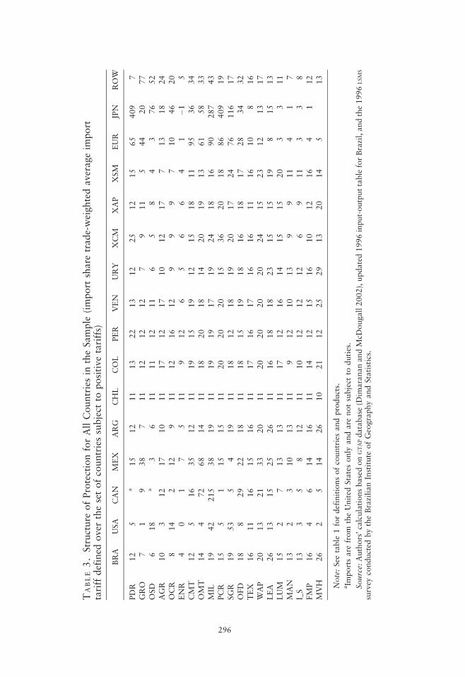
TABLE3.Structure

ofProtectionforAllCountriesin

theSample

(import

share

trade-weightedaverageim

port

tariffdefined

over

thesetofcountriessubject

topositivetariffs)

BRA

USA

CAN

MEX

ARG

CHL

COL

PER

VEN

URY

XCM

XAP

XSM

EUR

JPN

ROW

PDR

12

5a

15

12

11

13

22

13

12

25

12

15

65

409

7GRO

71

938

711

12

12

12

79

11

544

20

77

OSD

618

a3

611

11

12

11

65

84

376

52

AGR

10

312

17

10

11

17

12

17

10

12

17

713

18

24

OCR

814

212

911

12

16

12

99

97

10

46

20

ENR

40

17

511

912

65

66

41

�1

5CM

T12

516

35

12

11

19

15

19

12

15

18

11

95

36

34

OM

T14

472

68

14

11

18

20

18

14

20

19

13

61

58

33

MIL

19

42

215

38

19

11

19

19

17

19

24

18

16

90

287

43

PCR

15

51

15

15

11

20

20

20

15

36

20

18

86

409

19

SGR

19

53

54

19

11

18

12

18

19

20

17

24

76

116

17

OFD

18

829

22

18

11

18

15

19

18

16

18

17

28

34

32

TEX

16

11

16

15

16

11

17

16

17

16

16

11

16

10

816

WAP

20

13

21

33

20

11

20

20

20

20

24

15

23

12

13

17

LEA

26

13

15

25

26

11

16

18

18

23

15

15

19

815

13

LUM

15

27

13

13

11

17

12

16

14

15

15

20

33

11

MAN

13

23

10

13

11

912

10

13

99

11

41

7I_S

13

35

812

11

10

12

12

12

69

11

33

8FM

P16

46

14

16

11

14

12

15

16

10

12

16

41

12

MVH

26

25

14

26

10

21

12

25

29

13

20

14

513

Note:See

table

1fordefinitionsofcountriesandproducts.

aIm

portsare

from

theUnited

Statesonly

andare

notsubject

toduties.

Source:Authors’calculationsbasedon

GTAPdatabase

(Dim

arananandM

cDougall2002),updated1996input-outputtableforBrazil,andthe1996

LSMS

survey

conducted

bytheBrazilianInstitute

ofGeographyandStatistics.

296

The policy simulations are also performed with lower elasticity values ofsMM=8 and sDM=4.11 Lower elasticities typically lower the welfare gains forthe countries that gain from the regional arrangements and reduce the losses forcountries excluded from the regional arrangements, but they rarely change thequalitative results in the scenarios examined.12 Similarly, results at the house-hold level in Brazil are muted with lower elasticities, but the relative gains to thepoor in Brazil remain several multiples of the overall gain.

The elasticity of transformation between exports and domestic production isassumed to be 5 for each sector. Elasticities of substitution between primaryfactors of production is unity. Fixed coefficients are assumed between all inter-mediates and value added.

Protection Data

All distortions are represented as ad valorem price wedges. Border protectionestimates combine tariff protection and the tariff equivalents of nontariff bar-riers into a single measure of protection referred to as the tariff rate.

Trade in goods within Mercosur was tariff-free by 2000. Members wereallowed a list of exceptions to the common external tariff, but the commontariff is being phased in for the exceptions and all members are obligated to fullyconverge to it by 2006 (WTO 2000, p. 20). Because changes in protection dataare crucial to the results and protection rate data are usually available for amore recent period than input-output tables, the protection data used aretypically more recent than the data in the input-output tables.13 Similarly, tariffson imports of goods between Argentina, Brazil, and Uruguay are assumed to bezero. Because the common external tariff was largely in place in 2003 and isscheduled to be fully implemented by 2006, Argentina, Brazil, and Uruguay areall assumed to apply it.14

The North American Free Trade Association (NAFTA), too, is assumed tooperate as an effective free trade area, with zero tariffs between Canada,Mexico, and the United States, but with each country maintaining its ownexternal tariff. The model does not incorporate the preferential tariff rates

11. The results for low elasticites reported in Harrison and others (2003a) were erroneously reported

as being based on sMM=8 and sDM=4; in fact, they are based on sMM=16 and sDM=8.

12. The impact of unilateral trade liberalization on Argentina is one exception, for reasons explained

later.

13. Several sources of protection data were examined, and the data in the GTAP database were

assessed as the best. The trade flow data are also from the GTAP database, which is for 1997. Because

the input-output table and estimated factor payments in Brazil were updated, a balanced social account-

ing matrix (SAM) had to be created. An optimization procedure was employed in creating the new SAM that

minimizes the sum of the squares of the difference between all the values in the new SAM and the original

GTAP database, subject to the constraints of a SAM.

14. The common external tariff is imposed at the tariff-line level but is applied at the level of

aggregation of the model. This involves no loss of generality, because if the common external tariff

holds at the tariff-line level, then it must hold for more aggregate levels.


found in the many other regional trading arrangements in the Americas that areimplemented at various levels of effectiveness.

Table 3 shows the (trade-weighted) average protection rates by product cate-gory across all countries. The common external tariff of Mercosur is implementedby imposing the external tariff of Brazil as the external tariff of Argentina andUruguay. Nonetheless, the trade-weighted average tariff is not precisely equal in allcases for the three countries because of product mix differences across sources ofimports.

Brazilian Data for Poverty Analysis

Most of the data for Brazil, which are crucial to effective trade and povertyanalysis, were independently constructed for this study. In addition to theprotection data, the most important steps were to estimate factor shares inBrazilian industries, update the 1996 input-output table of the Brazilian eco-nomy from the 1985 base table in the GTAP database and use the householdexpenditure survey for Brazil to construct information on household expendi-ture patterns and sources of income.

The share of value added attributed to capital in input-output tables isnotoriously overestimated in agriculture and services and is poorly representedin many manufacturing sectors. The convention of input-output authorities is totake capital’s share as the residual from revenue after payments for intermedi-ates, labor, and taxes. Agriculture’s lack of official reported wage paymentsmeans that input-output authorities often report these sectors as the mostcapital-intensive sectors in the economy.15 Similar but less severe problemsprevail in services. In manufactures, unprofitable sectors (which often do notexport) have a low share of capital in the input-output tables, whereas profit-able sectors (which more often export) have a high share of capital. In devel-oping economies the result is that labor-intensive sectors, which may be themost profitable and export-oriented, are likely to be reported as capital-inten-sive sectors. Harrison and others (2003a) show how this problem can lead toperverse results.

Factor shares in Brazilian industries were thus independently estimated forthis study. The reestimation raised labor’s share significantly in agriculture and,to a lesser extent, in services. For manufactures there were no significantdifferences between these estimates and the input-output table. This adjustmentis fundamental to the results on the relative impact on the poor.

Household expenditure and income patterns were extracted from theLiving Standards Measurement Study (LSMS) survey for Brazil. The surveywas designed and conducted by the Brazilian Institute for Geography and

15. Researchers at the International Food Research Institute and the Economic Research Service of

the U.S. Department of Agriculture have noted this problem and adjusted for it (see Arndt and others

1998; Thomas and Bautista 1999; Hausner 1999; Burfisher and others 1992).


Statistics. The LSMS survey is a stratified sample, with each household represent-ing a share of the total population in the area sampled. The LSMS focused onthe eastern part of Brazil, but it is estimated to represent 103.6 million people inthe region (about 63 percent of the total population), 22.3 million of them inrural areas and 81.3 million in urban areas. Although much of the country isnot sampled in the survey, experts who have worked with the poverty data inBrazil believe that the poor are proportionally represented or at least are notunderrepresented.16 The Gini coefficient for the entire survey sample isestimated at 0.585.

To aggregate the approximately 5,000 Brazilian households in the survey into20 households, all households in the sample were first ranked from poorest torichest based on per capita income. Per capita rather than household incomewas chosen to enable comparisons with the standard per capita poverty mea-sures of the World Bank (World Bank 1990, 2000) and of Ferreira and others(1999) for Brazil. The sample was then divided into deciles, with an equalnumber of households in each decile (except for the richest decile, which hasmore households, because they were to receive less emphasis in the analysis).Each decile was then partitioned into two representative households: one ruraland one urban. This partition means that the ith representative rural householdand the ith representative urban household have about the same per capitaincome. Although the ith representative rural and the ith representative urbanhousehold do not have an equal number of households or individuals, the sumof the households they represent is equal, and the sum of individuals theyrepresent is approximately equal. As a result, there are roughly 1,800 indivi-duals in each household group, apart from the richest household group, whichhas just over 3,000 individuals (see table 2).

The shares of income each household spent on each commodity group andthe shares of income each household obtained from capital, rent on land,unskilled wages, and skilled wages were extracted from the LSMS survey. Dataon factor incomes were also available from national accounts, so the data fromthe two sources had to be reconciled before implementing the model.17 Forreasons to be explained, the total payments to factors were taken from thenational accounts, and the factor shares of each representative household in themodel were adjusted accordingly.18 This reconciliation minimized aggregatedeviations between household factor shares and expenditure shares from the

16. The authors thank Francisco Ferreira, Peter Lanjouw, and Marcelo Neri for helpful conversations

on several aspects of assessing poverty in Brazil.

17. A two-stage process in which price changes from a general equilibrium model are fed into a

second-stage micro-simulation model can ignore this reconciliation. Of course, inconsistencies then arise

if one then wants to allow for feedback from the second stage to the first stage after some policy shock.

18. This rebalancing also required adjusting expenditure shares of households for broad categories of

goods, to ensure consistency with the broad patterns of consumer expenditure in the national accounts.


values obtained from the LSMS survey prior to rebalancing, and the shares wereweighted by the value of household income and expenditure. The results arereported in table 4 and explained in Harrison and others (2003b, appendix D).

This reconciliation of the two databases significantly increased the share ofcapital owned by wealthy households, particularly wealthy urban households.Income estimates from LSMS surveys are known to be lower than income esti-mates from national accounts (see Ravallion 2003; Deaton 2003). Althoughthere are biases in collection of both databases, so that neither source is clearlycorrect, Deaton (2003) believes that the most likely explanation for the differ-ence is that households fail to respond to the survey, with the probability ofnonresponse increasing monotonically with income. It also appears to be thecase that the LSMS surveys report a lower share of income for capital than thenational accounts do. Vanos (2003) mapped income from the LSMS surveys in 14countries into factor shares and compared these with the GTAP database. Capi-tal’s share from the LSMS surveys was 21 percent of household income, but it was52 percent of household income based on national account information in theGTAP database. The presumed pattern of nonresponse to the household survey

TABLE 4. Household Income Shares from Factors of Production andTransfers (percent)

HouseholdType

SkilledLabor

Unskilledlabor

Rent fromCapital

Rent fromLand Transfers

Rural1 6 68 3 1 222 8 80 0 0 113 11 87 0 2 14 8 64 3 2 225 11 57 32 0 06 22 47 31 0 07 9 49 42 0 08 15 62 20 3 09 18 45 35 1 0

10 7 75 15 3 0

Urban1 1 70 0 0 282 18 67 1 0 143 10 74 3 0 144 13 68 8 0 105 27 57 16 0 16 28 52 19 0 07 27 30 42 0 08 33 28 39 0 09 30 21 49 0 0

10 17 15 69 0 0

Source: Authors’ calculations based on the 1996 LSMS survey conducted by the BrazilianInstitute of Geography and Statistics.


would also help explain this difference in capital’s share, because the rich arelikely to have more capital than the poor.19

What percentage of the households are poor based on the LSMS data? Povertylines are defined in several ways. Two well-known measures are $1 a day perperson or $2 a day per person at a purchasing power parity exchange rate. Fromthe LSMS data 7.3 percent of the population lives on $1 a day or less and 17.8percent lives on $2 a day or less. To calculate poverty in Brazil, Ferreira andothers (1999) developed a measure of poverty based on a ‘‘minimum foodbasket’’ in the reference region, metropolitan Sao Paulo, that would generatethe Food and Agriculture Organization–defined minimum intake of 2,288 cal-ories a day. They also developed indices that allow them to define ‘‘equivalent’’income levels across individual households in different regions of the LSMS. Usingpurchasing power parity adjustments for 1996, this measure amounts to apoverty line of $1.50 per person per day.20 Taking the poverty headcounts foreach region in Brazil as reported in Ferreira and others (1999, table 3) andsample weights for the individuals in each of the regions of the LSMS in Brazil,their measure implies a national poverty index of 13.03 percent for Brazil usingthe LSMS.21

Based on the Ferreira and others (1999) measure of poverty incidence and thefull LSMS database, 82 percent of the households in the poorest two households,urban household 1 and rural household 1, fall below this poverty line. Thepoorer households are more populous, however, so that this amounts to13 percent of the individuals in Brazil who are below the poverty line.22

I I . RESULTS AT THE COUNTRY LEVEL

The model estimates the aggregate change in welfare, measured by Hicksianequivalent variation, in Brazil and the other countries in the model as a result ofthe trade policy choices hypothetically made by Brazil (tables 5–7). The aggre-gate estimate of the change in welfare is the weighted sum of the welfarechanges for the 20 individual households in the model, reported as a percentage

19. In Brazil, capital’s share of factor income from the input-output tables is between 52 percent and

54 percent between 1995 and 1997. Capital’s share of factor income is 54 percent in the Brazilian Survey

of Industry for 1998 and 76 percent in the Brazilian Census of Agriculture for 1996. Factor shares in

production were reestimated to correct for biases in agriculture and services, so that capital’s share of

income is 50 percent based on the national accounts. But Vanos (2003) estimates capital’s share at 22

percent based on the LSMS survey. From our mapping of LSMS data, capital’s share is about 10 percent.

20. Specifically, they report a poverty level of 65.07 reals per month. This is divided by 30.417, the

average number of days in a month, and then further divided by 1.44 to get the purchasing power parity

equivalent in U.S. dollars. This is $1.48656, rounded to $1.50 for ease of recollection.

21. They also report comparable numbers from an alternative survey, known as the PPD, which imply

a national poverty index of 24.7 percent using comparable income measures.

22. The average number of people is 5.8 in rural household 1 and 5.0 in urban household 1. This

compares with an average of 3.9 for the entire survey.


TABLE5.Im

pact

ofMercosurTradePolicy

OptionsonSelectedCountriesAsaShare

ofConsumption,

CentralElasticities(w

elfare

change,

percent)

FTAA

FTAAwith

Excluded

Products

EU–M

ercosur

EU–M

ercosur

withExcluded

Products

FTAAand

EU–M

ercosur

Unilateral

50%

Tariff

Cut

Multilateral

Tariff

Liberalization

by50%

FTAAwith

noM

ercosur

Liberalization

Countryorregion

(1)

(2)

(3)

(4)

(5)

(6)

(7)

(8)

Brazil

0.6

0.4

0.9

0.1

1.8

0.4

0.9

0.4

Argentina

�0.2

�0.2

2.3

0.2

2.2

0.2

0.8

0.2

Uruguay

1.7

1.6

43.9

1.2

43.4

1.4

7.8

0.4

Chile

1.1

1.1

�0.2

0.0

0.9

0.1

1.3

0.8

Colombia

1.7

2.0

�0.1

�0.1

1.7

0.0

1.0

1.7

Peru

1.0

1.0

�0.1

0.0

0.9

0.0

1.3

1.0

Venezuela

1.1

1.1

0.0

�0.1

1.1

0.0

0.9

1.1

RestofAndeanpact

1.9

2.0

0.0

0.0

1.9

0.1

2.5

1.8

Mexico

0.3

0.4

0.0

0.0

0.3

0.0

0.5

0.0

CentralAmerica

andCaribbean

4.3

4.8

0.0

0.0

4.4

0.0

2.1

4.6

RestofSouth

America

0.8

0.8

�1.2

0.1

0.0

0.3

4.1

0.1

Canada

0.0

0.1

0.0

0.0

0.0

0.0

0.2

0.1

United

States

0.0

0.0

0.0

0.0

0.0

0.0

0.1

0.0

EuropeanUnion15

�0.1

0.0

0.5

0.1

0.4

0.0

0.8

�0.1

Japan

0.0

0.0

0.0

0.0

0.0

0.0

1.8

0.0

Restoftheworld

�0.1

�0.1

0.0

0.0

�0.1

0.0

2.3

�0.2

Note:

FTAAwith

excluded

products:

FTAAwith

U.S.antidumpingpolicy

denyingim

proved

accessto

itsfourprotected

sectors.EU-M

ercosurwith

excluded

products:afree

tradeagreem

entbetweenM

ercosurandtheEuropeanUnionwiththeseven

mostprotected

foodandagriculturalproductsin

the

EuropeanUnionexcluded

from

theagreem

ent.

FTAAandEU-M

ercosur:the

FTAAcombined

withafree

tradeagreem

entbetweenM

ercosurandtheEuropean

Union.Unilateral50%

tariffcut:aM

ercosur-only

tariffcutof50percent.M

ultilateraltariffliberalization:allregionsreduce

tariffsandexportsubsidiesby

50percent.

FTAAwithnoM

ercosurliberalization:the

FTAAbutM

ercosurdoes

notchangeitsexternaltariff

totherest

oftheAmericas.

Source:

Authors’computationsbasedon

GTAPdatabase

(Dim

arananandM

cDougall2002),updated1996input-outputtable

forBrazil,andthe1996

LSMSconducted



302

TABLE6.Im

pact


OptionsonSelectedCountries,CentralElasticities(w

elfare

gain

inbillionsof1996U.S.dollars) FTAA

FTAAwith

Excluded

Products

EU–M

ercosur

EU–M

ercosur

withexcluded

products

FTAAand

EU–M

ercosur

Unilateral

50%

Tariff

Cut

Multilateral

TariffLiberalization

by50%

FTAAwith

noM

ercosur

Liberalization

Country

(1)

(2)

(3)

(4)

(5)

(6)

(7)

(8)

Brazil

3.1

2.3

5.0

0.5

9.5

1.9

4.6

2.3

Argentina

�0.5

�0.5

5.9

0.5

5.7

0.5

2.0

0.5

Uruguay

0.2

0.2

6.5

0.2

6.4

0.2

1.2

0.1

Chile

0.5

0.6

�0.1

0.0

0.5

0.1

0.7

0.4

Colombia

1.1

1.3

�0.1

�0.1

1.1

0.0

0.6

1.1

Peru

0.4

0.4

0.0

0.0

0.4

0.0

0.6

0.4

Venezuela

0.7

0.7

0.0

0.0

0.7

0.0

0.5

0.6

RestofAndeanpact

0.4

0.4

0.0

0.0

0.4

0.0

0.5

0.3

Mexico

0.9

1.0

0.0

0.0

0.7

0.0

1.2

0.0

CentralAmericaandCaribbean

3.4

3.8

0.0

0.0

3.5

0.0

1.7

3.6

RestofSouth

America

0.1

0.1

�0.1

0.0

0.0

0.0

0.3

0.0

Canada

0.1

0.3

0.0

0.0

�0.1

0.0

0.8

0.2

United

States

2.3

2.0

�0.4

�0.4

1.7

0.3

3.0

�0.5

EuropeanUnion15

�2.6

�2.2

25.0

5.6

21.2

1.6

39.3

�3.2

Japan

�1.0

�0.9

0.7

0.4

�0.5

0.3

45.7

�1.2

Restoftheworld

�4.8

�4.2

�0.2

�0.2

�5.0

1.3

83.6

�5.6

Sum

forincluded

countries

12.7

12.4

42.3

6.9

51.6

NA

NA

9.1

Sum

forexcluded

countries

�8.4

�7.2

�0.2

�0.4

�5.5

NA

NA

�9.9

Sum

forallcountries

4.3

5.2

42.2

6.4

46.1

NA

186.0

�0.9

Note:

FTAAwith

excluded

products:

FTAAwith


denyingim

proved

accessto

itsfourprotected

sectors.EU-M

ercosurwith

excluded

products:afree

tradeagreem

entbetweenM


mostprotected


the


from

theagreem

ent.

FTAAandEU-M

ercosur:the

FTAAcombined

withafree

tradeagreem

entbetweenM


Union.Unilateral50percenttariff

cut:

aM

ercosur-only

tariff

cutof50percent.

Multilateraltariff

liberalization:allregionsreduce

tariffsandexport

subsidiesby50percent.

FTAAwithnoM


FTAAbutM

ercosurdoes

notchangeitsexternaltariff

totherest

oftheAmericas.

Source:


GTAPdatabase

(Dim

arananandM



LSMSconducted



303

TABLE7.Im

pact

ofTradePolicy

OptionsonMacroVariables,

CentralandLow

Elasticities(percentagechange)

FTAA

FTAAwith

Excluded

Products

EU–M

ercosur

EU–M

ercosur

withExcluded

Products

FTAAand

EU–M

ercosur

Unilateral

50%

Tariff

Cut

Multilateral

Tariff

Liberalization

by50%

FTAAwith

noM

ercosur

Liberalization

Macrovariable

Elasticity

(1)

(2)

(3)

(4)

(5)

(6)

(7)

(8)

Realexchangerate

Central

2.61

2.73

2.25

2.70

3.00

1.97

1.43

�0.2

Low

1.86

2.01

1.08

1.89

1.98

1.82

1.20

1.9

Changein

tariff

revenue

Central

0.60

0.56

0.56

0.55

0.69

0.10

0.12

0.0

(%ofGDP)

Low

0.52

0.50

0.50

0.48

0.72

0.20

0.24

0.5

Unskilledlaborwagerate

Central

2.91

1.87

4.24

2.42

5.81

0.94

3.02

0.0

Low

1.61

1.05

2.51

1.38

3.64

0.73

2.04

0.7

Skilledlaborwagerate

Central

0.97

1.01

1.12

0.60

1.77

0.54

0.31

1.1

Low

0.66

0.65

0.85

0.44

1.37

0.46

0.48

1.6

Rentalrate

oncapital

Central

�0.13

0.18

�0.47

�0.39

�0.31

�0.08

�0.59

�0.1

Low

0.17

0.32

0.00

�0.04

0.22

0.10

�0.09

0.2

Rentalrate

onland

Central

14.21

9.19

25.12

14.84

31.00

5.79

30.00

4.4

Low

6.31

3.94

13.19

7.38

16.76

3.56

16.27

6.3

Note:

FTAAwith

excluded

products:

FTAAwith


denyingim

proved

accessto

itsfourprotected

sectors.EU-M

ercosurwith

excluded

products:afree

tradeagreem

entbetweenM


mostprotected


the


from

theagreem

ent.

FTAAandEU-M

ercosur:theFTAAcombined

withafree

tradeagreem

entbetweenM



cut:

aM

ercosur-only

tariff

cutof50percent.

Multilateraltariff


tariffsandexport


FTAAwithnoM


FTAAbutM

ercosurdoes

notchangeitsexternaltariffto

therest

oftheAmericas.

Source:


GTAPdatabase

(Dim

arananandM



LSMSconducted



304

of consumption and in 1996 U.S. dollars. The central elasticity results arepresented explicitly, and important differences with low elasticities are alsomentioned. Key macrovariables that are important for the interpretation ofthe household results are presented in table 7.

Regional Arrangements

As part of Mercosur, Brazil is negotiating participation in the FTAA as well as anEU–Mercosur free trade agreement. Brazil will gain an estimated 0.6 percent ofpersonal consumption from the FTAA (about $3 billion; see tables 5 and 6,column 1). The gains to Brazil from a Mercosur–EU agreement are about 1.5times greater.

Both the FTAA and the EU–Mercosur agreement create very large economicareas, each with one large industrial country partner. These partners haveexport supply capacities that are large relative to the demand from smallerpartners. For a given absolute change in demand resulting from a regionalagreement, the larger capacity of these partner countries allows them to supplytheir smaller partners with relatively elastic supply curves. This prevents thesupply price for imports from large partner countries from rising significantly.Finally, large countries offer improved market access, as emphasized in Harrisonand others (1997a, 2002). Although in several cases preferential arrangementsamong small countries have been found to be welfare reducing,23 for the reasonsjust mentioned the estimates show that Brazil and most countries in the Americaswould gain from an FTAA and thatMercosur countries would gain from a free tradeagreement with the European Union.

The one exception to this pattern in the Americas is Argentina, which isestimated to lose slightly from the FTAA. Without FTAA it enjoys preferentialaccess to the markets of the other Mercosur countries. The FTAA providesequivalent access to the other countries in the Americas to the Mercosur market,eroding Argentina’s preferential access. The effects of this loss of preferentialaccess plus the trade diversion effects are larger than the trade creation effects.24

The combined gains to Argentina, Brazil, and Uruguay are more than 50 per-cent larger from an EU–Mercosur agreement than from the FTAA (see tables 5 and6, column 3). The European Union has several agricultural and food productswith very high tariffs (see table 2). If Argentina, Brazil, and Uruguay obtain tariff-free access to these markets while the European Union continues to apply thesetariffs on other countries, the three countries would receive large terms of tradegains in EU markets. The gains for Uruguay, a relatively small economy, would

23. See Harrison and others (2002) and Bakoup and Tarr (2000). Uruguay also loses from participa-

tion in Mercosur.

24. Pereira (1999) and Teixera and others (2002) find the same result for Argentina in the FTAA.

Although the gains to Brazil from the FTAA are also eroded because of erosion of preferential access in

Argentina, Argentina is a smaller market than the Brazilian market. Thus the erosion of preferential

access in the partner’s market is more important for Argentina.


be between 6 percent (with low elasticities) and 44 percent (with the centralelasticities).25

Countries excluded from the agreements typically lose. The European Union,Japan, and the rest of the world all lose from the FTAA, for a combined loss of$8.4 billion (see table 6, column 1). The excluded countries suffer a decline indemand for their exports to the Americas as importers in the Americas shiftdemand toward suppliers from the Americas. Hence there is both a terms oftrade loss on sales that continue and an efficiency loss from having to shift toalternate markets or products. The European Union is estimated to lose $2.6billion, slightly more than the $2.3 billion the United States is estimated to gain.One exception is Japan under the EU–Mercosur agreement. Japan obtains asmall terms of trade improvement in the markets of the rest of the world ascountries included in that agreement shift their trade toward each other’smarkets. The gains to Japan, however, are very small and round to zero at thenearest 0.1 percent of Japan’s consumption.

The benefits to Brazil from these two agreements exceed the sum of thebenefits for each agreement separately. This is because the combined economicarea of the Americas plus the European Union is vast, so Brazil is the less likelyto face adverse terms of trade effects as a result of consuming a large share ofany exporter’s supply. Lost tariff revenues from diverting trade to partnercountries that are part of either agreement taken separately are reduced bycombining the two agreements. Thus negotiating an agreement with the Eur-opean Union in addition to the FTAA appears likely to increase the welfare gainsto Brazil.26

Limitations on Market Access: The Impact of Antidumping, Rulesof Origin, and EU Agriculture Exclusions

Although preferential trade arrangements with large industrial countries offerdeveloping economies the promise of increased access to large markets, inpractice limitations on improved access significantly reduce the benefits. TheEuropean Union has steadfastly refused to grant tariff-free access in its highlyprotected agricultural products in its association agreements with Central andEastern European countries, its customs union agreement with Turkey, and itsfree trade area agreements with various Mediterranean countries (Morocco,Tunisia). Hence it is a priori unlikely to offer such concessions to Mercosur

25. The gains to Uruguay come primarily from the meat sector. Attracted by the tariff umbrella of 95

percent tariffs in the large EU market, Uruguay will dramatically expand meat output and exports to the

European Union in the long run. Meat exports are a much more significant share of gross domestic

product in Uruguay than they are in Argentina or Brazil. Thus the welfare gain from an improvement in

the export price in the European Union in this sector can be expected to result in a larger welfare gain

than in Brazil or Argentina. It is likely, however, that such a large expansion of the meat sector would be

constrained by ‘‘specific factors’’ in Uruguay that were not modeled.

26. These results are similar to those Harrison and others (2002) found for the ‘‘additive regionalism’’

strategy of Chile, which yielded significantly larger benefits than the agreements taken separately.


when it has refused to offer them to countries for which it might be viewed ashaving more to gain geopolitically.

As for the FTAA, the United States has strongly resisted efforts to limit the useof antidumping actions as part of the FTAA despite a proposal by Chile to includesuch a limitation. As the use of tariffs and nontariff barriers has declined, the useof antidumping as a protectionist device has risen significantly in the UnitedStates (Finger 1993) (and more recently in the European Union as well; seeMesserlin and Reed 1995). Antidumping actions have focused on four sensitivesectors: chemicals, metals, nonelectrical machinery, and electrical equipment.Thus Brazilian authorities have expressed the fear that the benefits of nominallyimproved access to U.S. markets will be denied by antidumping actions.

Finally, free trade agreements involve rules of origin, requiring that exporterssource a share of inputs from within the preferential area. Evidence is accumu-lating that these rules of origin significantly limit the improved market access ofpreferential tariff concessions. The Africa Growth and Opportunity Act pro-vides preferential access for African exports to the U.S. markets. Mattoo andothers (2002) found that African nonoil exports to the United States wouldincrease by about 50 percent without the stringent rules of origin but by only 10percent with them. Estevadeordal (2000) found that restrictive rules of originlimited Mexico’s improved access to the U.S. market under NAFTA. Brenton andManchin (2003) argue that EU preferential trade agreements have been ineffec-tive in delivering improved market access, most likely because of the restrictiverules of origin and the costs of proving compliance.

Two simulations illustrate how these limitations of market access by theEuropean Union and the United States can affect the potential gains.

Excluded Agricultural Products in the EU–Mercosur Agreement. This sce-nario assumes that the European Union fails to provide improved market accessto its most highly protected agricultural products in an EU–Mercosur agree-ment. The EU tariff rates in the database are 65 percent for paddy rice, 44percent for cereal grains, 86 percent for processed rice, 28 percent for other foodproducts, 95 percent for bovine meat products, 90 percent for dairy products,61 percent for other meat products, and 76 percent for sugar. These areproducts in which the Mercosur countries have a comparative advantage, so ifthe free trade agreement between the European Union and Mercosur excludesthese products, the expected benefits would be significantly reduced.

Under the central elasticity results the denial of full market access to these keyagricultural products reduces the value of the EU–Mercosur agreement to Brazilfrom 0.9 percent of consumption to 0.1 percent (see tables 5 and 6, column 4).The estimated gains for Uruguay are also dramatically reduced. The gains to theEuropean Union are also reduced, from 0.5 percent of its consumption to 0.1percent, reflecting the importance of agriculture liberalization if EU consumersare to reap gains from the agreement.

Antidumping and Rules of Origin in the FTAA. Limitations on access to theU.S. market are more likely to come from restrictive rules of origin and the use


of antidumping actions than from explicit exclusion of certain products. Indeed,Brazilian authorities have expressed the fear that the benefits of improved accessto U.S. markets will be denied by antidumping actions, as in the steel sector.This scenario estimates the costs to Brazil of continued U.S. protection of its mostprotected markets even with the FTAA. Protection is 53 percent on sugar, 42 percenton dairy products, 18 percent on oil seeds, and 14 percent on other crops.27

For these sectors the United States is assumed to employ antidumping dutiesor stringent rules of origin to neutralize the impact of the FTAA on Brazil’sexports (in other words, the U.S. tariff on exports of these products from Brazildoes not change).28

The impact is to reduce the benefits to Brazil to about two-thirds of the gainsit would receive with full market access in the FTAA (see tables 5 and 6, column 2).The reduction is not as severe as with the excluded products in the EUagreement. The large impacts tend to be driven by the tariff peaks, which arenot as high in the U.S. market as in the European Union. If the United Statesfails to provide preferential access to its highly protected products, Brazil cansell these products in other markets in the Americas that also open up to Brazilon a preferential basis as part of the FTAA. With the EU–Mercosur agreementthere are no alternate markets in which Brazil has preferential access.

FTAA with No Change in Mercosur’s External Tariffs. To identify the source ofgains, especially at the household level, the impact of the FTAA with no improvedaccess to Mercosur markets is also evaluated. This scenario shows how much ofthe gains to Brazil come from improved access to the markets of the Americas andhow much from lowering Mercosur tariffs, thereby achieving improved resourceallocation in Brazil. In this scenario the countries in the Americas outside ofMercosur are assumed to lower their tariffs preferentially to all countries in theAmericas (so Brazil obtains improved market access), but the Mercosur countriesdo not lower their common external tariffs against partner countries in theAmericas (so Brazil does not offer any improved market access).

Under this scenario the gains to Brazil are reduced to 0.4 percent of con-sumption. This shows that improved market access is responsible for about two-thirds of the gain to Brazil from the FTAA and that the remaining one-third of thegain comes from the preferential lowering of the Mercosur tariff (see tables 5and 6, column 8).

27. The category ‘‘other crops’’ is an aggregate of the following sectors from the full GTAP data set:

wheat, vegetables and fruits, fiber-based plants, wool, forestry, fishing, and other crops. Simulations were

also performed with wheat as part of grains rather than other crops. Argentina gains more from the EU–

Mercosur agreement, but otherwise most of the results change by very small amounts.

28. This is not a full treatment of the potential use of antidumping or rules of origin within the FTAA

or of the impact on Brazil. Such treatment would have to account for antidumping duties and stringent

rules of origin by the United States against other products and partners in the Americas as well and for the

use of antidumping and stringent rules of origin by countries other than the United States.


Tariff Cuts and Uniformity in Mercosur or Multilateral Liberalization—or Both

Simulations were also run for unilateral tariff cuts by Mercosur and for cutsthrough multilateral trade liberalization under the WTO.

Unilateral Trade Liberalization by 50 Percent and Tariff Uniformity. A50 percent cut in Mercosur tariffs will result in a welfare increase of about0.4 percent of Brazilian consumption or about $1.9 billion a year (see tables 5and 6, column 6). Thus the gains from the FTAA with excluded access to the U.S.market on selected products results in about the same gains as a unilateral tariffcut by Mercosur of 50 percent. With low elasticities, however, the gains are onlyabout 0.2 percent of consumption for Brazil, or $0.4 billion, and the impact onArgentina is negative.29 The larger terms of trade effects with the lower elasti-cities account for the lower gains from tariff reduction.

Tariff uniformity (with the same collected tariff revenue) in Mercosur willresult in slightly larger welfare gains than a 50 percent cut in tariffs. Theseresults are consistent with earlier results on the benefits of tariff uniformity forTurkey and Chile (Harrison and others 1993, 2002). Similarly, Martinez dePrera (2000) found welfare gains from tariff uniformity in all 13 countriesevaluated. Although theory indicates that taxes are more efficient if they arehigher on products with relatively low elasticities of demand, evidently tariffs donot typically differ from uniformity in these economies for tax efficiency rea-sons.30 On the contrary, the large gains from trade liberalization typically comefrom reducing tariff peaks, which is effectively accomplished through tariffuniformity. Reducing low tariffs results in proportionately smaller gains andmay even result in losses if the importing country possesses monopsony power.

Multilateral Trade Liberalization. Brazilian authorities have also encouragedmultilateral trade negotiations and supported the Doha Development Agenda—in part because of a belief that it is the most likely way to achieve agriculturalliberalization. In this scenario all countries in the world reduce their tariffs andexport subsidies and their taxes by 50 percent.

Brazil gains about 0.9 percent of personal consumption from multilateraltrade liberalization in the static model, or about $4.6 billion a year (see tables 5and 6, column 7). These are larger than the gains from the FTAA and those froman agreement with the European Union that excludes the highly protected

29. Harrison and others (1997c, appendix C) show that the optimal tariff t in any sector of the model

is bounded below by t*= {[sMM/(sMM – 1)] – 1}. Thus even in the central elasticity case with sMM = 30 the

optimal tariff is more than 3 percent. But in the low elasticity scenarios, with sMM = 8, the optimal tariff

is more than 14 percent. With an average Mercosur tariff of 12 percent, the optimum uniform tariff is

lower than the existing average tariff in the central elasticity scenarios. The small gains that remain are

due to lowering the tariff peaks.

30. The set of elasticities that were chosen, however, makes uniformity beneficial in general. That is,

the Ramsey optimal taxation rule suggests that higher taxes should be placed on goods with the lower

elasticity of demand. With the virtually homogeneous choice of elasticities here, the Ramsey optimal

tariffs are close to uniform.


agricultural and food products. Because these products are likely to be excludedfrom a Mercosur agreement with the European Union, the results support thestrategy of the Brazilian authorities to pursue multilateral liberalization alongwith the regional options.

The gains to the world from the 50 percent cut in tariffs and export subsidiesare estimated at $186 billion with central elasticities (see table 6, column 7) and$87 billion with low elasticities. As Harrison and others (1997b) argue inassessing the Uruguay Round, elasticities play an important role in explainingdifferences in aggregate gains from multilateral trade liberalization.

IMPACT ON HOUSEHOLDS AND THE POOR

The household results follow a similar pattern across all of the policy scenarios(table 8). The poorest household will typically gain several times the aggregategains for the economy expressed as a percentage of household consumption.31

Although the impact on household incomes is not strictly progressive, the fourpoorest urban households and four poorest rural households are among the biggestgainers from the reforms as a percentage of their own household consumption.

What accounts for this robust and encouraging result? Trade protection inBrazil favors capital-intensive manufactures, so liberalization shifts resourcestoward more unskilled labor-intensive agriculture. Thus the wage rate of unskilledlabor increases significantly more that the rent on capital (see table 7).32 Thepoorest households earn most of their income from unskilled labor (see table 4),so they gain proportionally more than other households.

Although the impact on sectors depends on the specific agreement, there is ageneral pattern. Oilseeds, other agriculture (excluding grains and wheat), othercrops (which includes fruits and vegetables and wheat), processed food, andleather sectors expand production and exports. These sectors, especially theagricultural sectors,33 are the most intensive users of unskilled labor in themodel. Several manufacturing sectors decline, including motor vehicles, othermetal products, and other manufacturing. These declining sectors are among themost capital-intensive in Brazil.

These outcomes reflect relative protection in Brazil, which favors manufac-turing at the expense of agriculture and processed food products. Despitesubstantial trade liberalization, vestiges of Brazil’s import-substitution indus-

31. The percentage gains for the poor relative to the aggregate percentage gains are similar for low

trade elasticities.

32. The poor typically have not accumulated large stores of real assets or financial assets, so they do

not earn significant capital income or income from the rent of land. Nor have the poor typically

accumulated much human capital, so they earn a much smaller share of their income from skilled

labor than do the middle classes.

33. The EU–Mercosur agreement (without exceptions) induces a much larger increase in agricultural

output in Brazil than do the other agreements because of the large increase in preferential access for

Mercosur countries in the European Union.


TABLE8.Im

pact


OptionsonBrazilianHouseholdsasaShare

ofConsumption,CentralElasticities

(welfare

change,

%)

Household

FTAA

FTAAwith

Excluded

Products

EU–M

ercosur

EU–M

ercosur

withExcluded

Products

FTAAand

EU–M

ercosur

Unilateral

50%

Tariff

Cut

MultilateralTariff

Liberalization

by50%

FTAAwith

noM

ercosur

Liberalization

type

(1)

(2)

(3)

(4)

(5)

(6)

(7)

(8)

Rural

12.5

1.7

4.0

2.1

5.5

1.5

2.9

0.8

22.3

1.5

3.9

1.8

5.4

1.2

2.8

1.0

32.5

1.5

4.5

1.9

6.2

1.1

3.5

1.3

42.5

1.8

3.9

2.2

5.4

1.5

3.1

0.8

51.3

0.8

2.3

0.7

3.5

0.6

1.8

0.8

61.5

1.0

2.3

0.8

3.6

0.7

1.7

0.8

71.3

0.9

2.0

0.7

3.2

0.6

1.6

0.7

83.1

2.0

4.8

2.4

6.9

1.2

4.1

1.4

90.9

0.4

1.7

0.6

2.6

0.4

1.8

0.7

10

3.7

2.3

6.0

2.8

8.3

1.4

4.9

1.6

Urban

12.5

1.8

3.8

2.1

5.2

1.5

2.7

0.7

22.3

1.6

3.8

1.8

5.2

1.3

2.6

0.8

32.2

1.4

3.6

1.7

5.0

1.2

2.6

0.9

42.0

1.3

3.1

1.5

4.5

1.0

2.4

0.8

51.3

0.7

2.4

0.8

3.5

0.7

1.8

0.8

61.6

1.0

2.6

1.0

3.9

0.7

1.9

0.8

70.4

0.3

0.9

0.0

1.6

0.3

0.7

0.4

80.3

0.2

0.7

�0.1

1.4

0.3

0.7

0.4

9�0.5

�0.4

�0.3

�0.7

�0.1

0.0

0.1

0.2

10

0.0

0.2

�0.2

�0.5

0.5

0.1

0.0

0.2

Note:

FTAAwithexcluded

products:

FTAAwithU.S.antidumpingpolicy

denyingim

proved

accessto

itsfourprotected

sectors.EU-M

ercosurwith

excluded

products:afree

tradeagreem

entbetweenM


mostprotected


the


from

theagreem

ent.

FTAAandEU-M

ercosur:theFTAAcombined

withafree

tradeagreem

entbetweenM



cut:

aM

ercosur-only

tariff

cutof50percent.M

ultilateraltariff


tariffsandexport


FTAAwithnoM


FTAAbutM

ercosurdoes

notchangeitsexternaltariffto

therest

oftheAmericas.

Source:


GTAPdatabase

(Dim

arananandM



LSMSconducted



311

trialization protection structure remain. When protection in the economy isreduced, resources shift toward the agriculture and food sectors that had beendisadvantaged relative to manufacturing. The expanding sectors tend to be lesscapital-intensive than the contracting sectors. International trade theory arguesthat the price of the factor of production used intensively in protected sectorsshould fall relative to the price of the factor of production in the unprotectedsectors following trade liberalization.34 Thus the wage rate of unskilled laborrises relative to the rent on capital, benefiting the poor. Because the value ofland rises even more than the wage rate of unskilled labor, two of the richestrural households are the biggest gainers from the reforms.

To document this interpretation of why the poor can be expected to gainproportionally more than wealthier households, the impact of the FTAA onhouseholds was decomposed in table 9. Column 1 reproduces the base resultsfrom table 8 for the FTAA. Column 2 presents the results of assuming that allhouseholds consume the commodities in the same proportions. Although thegains to the poorest households decline slightly, they remain three to four timesgreater than the percentage gains for all households together. Thus, disparateconsumption shares do not explain why poor households gain more from thetrade policy changes.

Column 3 presents the results of the FTAA scenario in which all households areassumed to earn the same shares of income from the wages of unskilled laborand skilled labor and rent on capital and land. Most of the poorest householdswould obtain only a slightly greater increase in income than the average for allhouseholds of 0.6 percent. This confirms that it is the more than proportionaterise in the price of the factors of production important to the income of poorhouseholds that explains why poor households gain more from these tradepolicy options. The factor most important to the poor is the wage rate ofunskilled labor (see table 4), which rises fastest among the important householdincome factors (see table 7).

An additional simulation offers further support for this explanation. Forreasons explained earlier, the capital intensity in agriculture sectors is estimatedto be significantly less than reported in the Brazilian input-output table. There isa dramatic difference in the results for the estimated welfare gains from the FTAA

to Brazilian households when the biased factor shares in the GTAP data are usedinstead of the corrected data. The poorest rural household is estimated to gain0.5 percent of its consumption and the poorest urban household 0.4 percent,equal or slightly less than the aggregate average percentage gain (see table 9,column 4). This shows that the corrections to the factor share data are crucial tothe results at the household level and supports the interpretation that the shift of

34. This is known as the Stolper-Samuelson theorem. In this model, however, product differentiation

mutes strict application of the Stolper-Samuelson results.


resources toward agriculture is important in increasing the incomes of the poorand reducing poverty.

The results also show that the Mercosur tariff changes are more important tothe poor than improved market access (see tables 5 and 8, column 8). In thisscenario Mercosur does not change its own tariffs but obtains improved accessto the markets of the Americas. The average gains to the economy fall by aboutone-third compared with the FTAA gains, but the gains to the poorest householdsfall by two-thirds. This is because Mercosur’s tariff changes induce outputexpansion in the sectors that intensively use unskilled labor, thus increasingunskilled wages relative to other factor prices. Improved market access does notincrease the price of unskilled labor relative to capital. With only improvedmarket access, the poor gain, but not progressively as they do with internalliberalization in Mercosur.

TABLE 9. Decomposition of the Impact of the FTAA on Brazilian Householdsas a Share of Consumption, Central Elasticities (change in welfare, %)

FTAA

FTAA with UniformConsumption

SharesFTAA with UniformIncome Shares

FTAA with FactorShares from

Input-Output Table

(1) (2) (3) (4)

All households 0.6 0.6 0.6 0.5Rural1 2.5 2.0 1.0 0.52 2.3 1.8 0.7 0.33 2.5 2.0 0.5 0.14 2.5 2.1 0.9 1.05 1.3 0.8 0.5 0.46 1.5 0.7 0.9 0.77 1.3 0.6 0.7 0.58 3.1 2.8 1.0 2.29 0.9 1.2 0.0 0.810 3.7 3.2 1.1 2.0

Urban1 2.5 2.0 1.0 0.42 2.3 1.8 0.9 0.23 2.2 1.8 0.7 0.04 2.0 1.6 0.7 0.95 1.3 1.0 0.3 0.16 1.6 1.4 0.6 0.47 0.4 0.2 0.3 0.18 0.3 0.3 0.2 0.09 �0.5 0.0 �0.3 �0.310 0.0 0.1 0.9 0.9

Source: Authors’ computations based on GTAP database (Dimaranan and McDougall 2002),updated 1996 input-output table for Brazil, and the 1996 LSMS conducted by the Brazilian Instituteof Geography and Statistics.


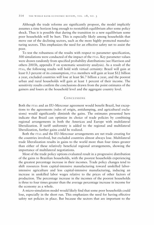
Although the trade reforms are significantly propoor, the model implicitlyassumes a time horizon long enough to reestablish equilibrium after some policyshock. Thus it is possible that during the transition to a new equilibrium somepoor households will be hurt. This is especially likely among households thatmove out of the declining sectors, such as the more highly protected manufac-turing sectors. This emphasizes the need for an effective safety net to assist thepoor.

To test the robustness of the results with respect to parameter specification,500 simulations were conducted of the impact of the FTAA. Key parameter valueswere drawn randomly from specified probability distributions (see Harrison andothers 2003b, appendix F on systematic sensitivity analysis). As a result of theFTAA, the following results will hold with virtual certainty: Brazil will gain atleast 0.3 percent of its consumption, FTAA members will gain at least $12 billiona year, excluded countries will lose at least $6.7 billion a year, and the pooresturban and rural households will gain at least 1 percent of their income. Thesensitivity results confirm the conclusions drawn from the point estimates of thegainers and losers at the household level and the aggregate country level.

CONCLUS IONS

Both the FTAA and an EU–Mercosur agreement would benefit Brazil, but excep-tions to the agreements (rules of origin, antidumping, and agricultural exclu-sions) would significantly diminish the gains. The estimates presented hereindicate that Brazil can optimize its choice of trade policies by combiningregional arrangements in both the Americas and Europe with multilateralliberalization. If tariff uniformity is added to the regional and multilateralliberalization, further gains could be realized.

Both the FTAA and the EU–Mercosur arrangements are net trade creating forthe countries involved, but excluded countries almost always lose. Multilateraltrade liberalization results in gains to the world more than four times greaterthan either of these relatively beneficial regional arrangements, showing theimportance of multilateral negotiations.

Most of the trade policy options evaluated result in a progressive distributionof the gains to Brazilian households, with the poorest households experiencingthe greatest percentage increase in their incomes. Trade policy changes tend toshift resources from capital-intensive manufacturing toward unskilled labor-intensive agriculture and less capital-intensive manufacturing, inducing anincrease in unskilled labor wages relative to the prices of other factors ofproduction. The percentage increase in the incomes of the poorest householdsis three to four times greater than the average percentage increase in income forthe economy as a whole.

A micro-simulation model would likely find that some poor households couldlose, especially in the short run. This emphasizes the need for having effectivesafety net policies in place. But because the sectors that are important to the


poor tend to be disfavored by the structure of protection, the medium- to long-run effects of these trade reforms should be positive for the vast majority of thepoorest households.

REFERENCES

Adelman, Irma, and Sherman Robinson. 1978. Income Distribution Policies in Developing Countries.

Stanford, Calif.: Stanford University Press.

Athukorala, Premachandra, and James Reidel. 1994. ‘‘Demand and Supply Factors in the Determination

of NIE Exports: A Simultaneous Error-Correction Model for Hong Kong: A Comment.’’ Economic

Journal 104(427):1411–14.

Arndt, C., A. Cruz, H. T. Jensen, S. Robinson, and F. Tarp. 1998. ‘‘Social Accounting Matrices for

Mozambique 1994 and 1995.’’ TMD Discussion Paper 28. International Food Policy Research Insti-

tute, Trade and Macroeconomics Division, Washington D.C.

Bakoup, Ferdinand, and David Tarr. 2000. ‘‘The Economic Effects of Integration in the Central African

Economic and Monetary Community: Some General Equilibrium Estimates for Cameroon.’’ African

Development Review 12(3):161–90.

Barros, R. P., C. H. Corseuil, and S. Cury. 2000. ‘‘Trade Opening and Liberalization of Capital Flows in

Brazil: Impacts on Poverty and Inequality.’’ In R. Henriques, ed., Desigualdade e pobreza no Brasil.

Rio de Janeiro: Instituto de Pesquisa Economica Aplicada.

Brenton, Paul, and Meriam Manchin. 2003. ‘‘Making EU Trade Agreements Work: The Role of Rules of

Origin.’’ World Economy 26(5):755–69.

Burfisher, M., K. Thierfelder, and K. Hanson. 1992. ‘‘Data Base for a Computable General Equilbrium

Model of the Agricultural Sectors of the United States and Mexico and Their Interaction.’’ Staff

Report AGES9225. U.S. Department of Agriculture, Economic Research Service, Washington, D.C.

Bussolo, Maurizio, and Jann Lay. 2003. ‘‘Globalization and Poverty Changes in Columbia.’’ Paper

presented at the Annual World Bank Conference on Development Economics, Europe, May 15–16,

Paris.

Chang, Won, and L. Alan Winters. 2002. ‘‘How Regional Blocs Affect Excluded Countries: The Price

Effects of Mercosur.’’ American Economic Review 92(4):889–904.

Chen, Shaohua, and Martin Ravallion. 2003. ‘‘Household Welfare Impacts of China’s Accession to the

WTO.’’ World Bank, Washington, D.C.

Cockburn, John. 2001. ‘‘Trade Liberalization and Poverty in Nepal: A Computable General Equilibrium

Micro Simulation Analysis.’’ CREFA Working Paper 01-18. University of Laval, Center for Applied

Economic and Financial Research, Quebec. Available online at www.crefa.ecn.ulaval.ca/cahier/

0119.pdf.

Deaton, Angus. 2003. ‘‘Measuring Poverty in a Growing World (or Measuring Growth in a Poor

World).’’ Working Paper, Princeton University, Department of Economics. Available online at

www.wws.princeton.edu/�deaton/working.htm.

de Melo, Jaime, and David Tarr. 1992. General Equilibrium Analysis of U.S. Foreign Trade Policy.

Cambridge, Mass.: MIT Press.

Dimaranan, Betina V., and Robert A. McDougall. 2002. Global Trade, Assistance, and Production: The

GTAP 5 Data Base. Purdue University, Center for Global Trade Analysis. Available online at www.gta-

p.agecon.purdue.edu/databases/v5/v5_doco.asp.

Estevadeordal, Antoni. 2000. ‘‘Negotiating Market Access.’’ Journal of World Trade 34(1):141–66.

Ferreira, Francisco H. G., Peter Lanjouw, and Marcelo Neri. 1999. ‘‘The Urban Poor in Brazil in 1996: A

New Poverty Profile Using PPV, PNAD and Census Data.’’ Unpublished manuscript. World Bank,

Washington, D.C.

Ferris, M. C., and T. S. Munson. 2000. ‘‘Complementarity Problems in GAMS and the PATH Solver.’’

Journal of Economic Dynamics and Control 24(2):165–88.


Finger, J. Michael, ed. 1993. Antidumping: How It Works and Who Gets Hurt. Ann Arbor: University of

Michigan Press.

Harrison, Glenn W., Thomas F. Rutherford, and David Tarr. 1993. ‘‘Piecemeal Trade Reform in the

Partially Liberalized Economy of Turkey.’’ World Bank Economic Review 7(2):191–217.

———. 1997a. ‘‘Economic Implications for Turkey of a Customs Union with the European Union.’’

European Economic Review 41(3–5):861–70.

———. 1997b. ‘‘Quantifying the Uruguay Round.’’ Economic Journal 107(444):1405–30.

———. 1997c. ‘‘Trade Policy Options for Chile: A Quantitative Evaluation.’’ Policy Research Working

Paper 1783. World Bank, Washington, D.C. Available online at www.worldbank.org/research/trade/

archive.html.

———. 2002. ‘‘Trade Policy Options for Chile: The Importance of Market Access.’’ World Bank

Economic Review 16(1):49–79.

———. 2003a. ‘‘Trade Liberalization, Poverty and Efficient Equity.’’ Journal of Development Economics

71(1):97–128.

Harrison, Glenn W., Thomas F. Rutherford, David G. Tarr, and Angelo Gurgel. 2003b. ‘‘Regional,

Multilateral and Unilateral Trade Policies of Mercosur for Growth and Poverty Reduction in Brazil.’’

Policy Research Working Paper 3051. World Bank, Washington, D.C. Available online at

www.worldbank.org/research/trade.

Hausner, U. 1999. ‘‘A 1995 Social Accounting Matrix for Zambia.’’ TMD Discussion Paper Series 49.

International Food Policy Research Institute, Trade and Macroeconomics Division, Washington, D.C.

Martinez de Prera, Josefina. 2000. ‘‘Revenue-Neutral Tariff Reform: Welfare Effects of Uniform Tariffs

in 13 Developing Countries.’’ PhD dissertation. University of Colorado, Department of Economics.

Available online at http://ussub.colorado.edu/�martindp.

Mattoo, Aaditya, Devesh Roy, and Arvind Subramaniam. 2002. ‘‘The Africa Growth and Opportunity

Act and Its Rules of Origin: Generosity Undermined?’’ Policy Research Working Paper 2908. World

Bank, Washington, D.C. Available online at www.worldbank.org/research/trade/archive.html.

Mattoo, Aaditya, Carsten Fink, Mario Marconini, and Lia Valls Pereira. 2002. ‘‘Brazil’s Services Trade

and International Trade Negotiations.’’ Working Paper. World Bank, Washington, D.C.

Messerlin, Patrick, and Geoffrey Reed. 1995. ‘‘Antidumping Policies in the United States and the

European Community.’’ Economic Journal 105(433):1565–75.

Muendler, Mark-Andreas. 2001. ‘‘Trade, Technology, and Productivity: A Study of Brazilian Manufac-

turers: 1986–98.’’ Working Paper. University of California, Department of Economics, Berkeley.

Pereira, Lia Valls. 1999. ‘‘Estudo sobre linhas estrutuais da posicao brasileira, nos principais setores

produtivos, de interesse do Brasil, no ambito do exercicio de conformacao da ALCA no ambito das

negociacoes do Mercosul com a uniao Europeia.’’ Fundacao Getulio Vargas, o Ministerio de Desen-

volvimento, Industria e Comercio do Brasil.

Piggott, John, and John Whalley. 1985. UK Tax Policy and Applied General Equilibrium Analysis. New

York: Cambridge University Press.

Ravallion, Martin. 2003. ‘‘Measuring Aggregate Welfare Effects in Developing Countries: How Well Do

National Accounts and Surveys Agree?’’ Review of Economics and Statistics 85(3):645–52.

Reidel, James. 1988. ‘‘The Demand for LDC Exports of Manufactures: Estimates from Hong Kong.’’

Economic Journal 98(389):138–48.

Reinert, Kenneth A., and David W. Roland-Holst. 1992. ‘‘Armington Elasticities for United States

Manufacturing Sectors.’’ Journal of Policy Modelling 14(5):631–39.

Roland-Holst, David, and Dominique van der Mensbrugghe. 1992. ‘‘Trade Liberalization in the Americas:

Are Regionalism and Globalization Compatible?’’ Paper presented at the conference on the Impact

of Trade Liberalization Agreements on Latin America and the Caribbean, November 5–6, Inter-

American Development Bank and Centre d’Etudes Prospectives et d’Information Internationales,

Washington, D.C.


Rutherford, Thomas F. 1999. ‘‘Applied General Equilibrium Modeling with MPSGE as a GAMS Subsystem:

An Overview of the Modeling Framework and Syntax.’’ Computational Economics 14(1/2):1–46.

Rutherford, Thomas F., and David G. Tarr. 2002. ‘‘Trade Liberalization, Product Variety and Growth in

a Small Open Economy: A Quantitative Assessment.’’ Journal of International Economics 56(2):

247–72.

Shiells, C. R., and K. A. Reinert. 1993. ‘‘Armington Models and Terms-of-Trade Effects: Some Econo-

metric Evidence for North America.’’ Canadian Journal of Economics 26(2):299–316.

Teixera, Erly, Luiz Cypriano, and Wildson Pinto. 2002. ‘‘Impacts of AFTA and MERCOEURO on Agribusiness

in the MERCOSUL Countries.’’ Paper presented at the Fifth Annual Conference on Global Economic

Analysis, June 5–7, Taipei, Taiwan, China. Available online at www.gtap.agecon.purdue.edu/

resources/res_display.asp?recordid= 1017.

Thomas, M., and M. Bautista. 1999. ‘‘A 1991 Social Accounting Matrix (SAM) for Zimbabwe.’’ TMD

Discussion Paper 36. International Food Policy Research Institute, Trade and Macroeconomics

Division, Washington, D.C.

Vanos, Maros. 2003. ‘‘Reconciliation of the GTAP and Household Survey Data.’’ Working Paper. Purdue

University, Department of Agricultural Economics. Available online at www.gtap.agecon.purdue.edu/

events/board_meetings/2003/docs/maros_survey.pdf.

World Bank. 1990. World Development Report 1990: Poverty. New York: Oxford University Press.

———. 2000.World Development Report 2000/2001: Attacking Poverty. New York: Oxford University

Press.

———. 2001. Rural Poverty Alleviation in Brazil: Towards an Integrated Strategy. Washington, D.C.:

World Bank.

WTO (World Trade Organization). Trade Policy Review, Brazil 2000. Geneva.


trade policy and poverty reduction in...

Documents