Trade receivables policy ofdistressed firms and its effecton the costs of financial distress

Carlos A. Molina andLorenzo A. Preve

Est

udio

IES

A N

° 25

Derechos exclusivos2006© IESAHecho el depósito de leyDepósito legal: lf23920063302136ISBN: 980-217-306-1

Para ser publicado como Estudio IESA un texto tiene que ser aprobado por el Comité de Publicaciones. Las opiniones expresadas son del autory no deben atribuirse al IESA, a sus directivos ni a Ediciones IESA. Para cualquier información sobre este estudio, favor dirigirse a EdicionesIESA, Apartado 1640, Caracas, Venezuela 1010-A. Teléfono: 58-212-555.44.52. Fax: 58-212-555-44-45. Dirección electrónica:ediesa@iesa.edu.ve.

Contents

Abstract...................................................................................................................................... 4Introduction............................................................................................................................... 5Data............................................................................................................................................. 6

The effect of financial distress on trade credit................................................................ 7The effect of market power and industry concentration............................................... 9Profitability problems and cash-flow problems.............................................................. 10The cost of cutting trade receivables................................................................................ 12

The cost of cutting trade receivables when firms are in financial distress................ 12

The effect of cutting trade receivables for highly leveraged firms in

distressed industries...................................................................................................... 13

Concluding remarks............................................................................................................... 14References................................................................................................................................ 16

Estudio IESA

4

AbstractThis paper studies the trade receivables policy of distressed firms as the tradeoff between a firm’s willingnessto gain sales and its need for cash. We find that firms increase trade receivables when they have profitabilityproblems prior to entering financial distress, but reduce trade receivables when they have cash-flow problemswhile undergoing financial distress. We also find that a firm that significantly cuts its trade receivables whenin financial distress will have an additional 7% drop in sales and stock returns over the previously documented24% average drop for a firm in financial distress. Moreover, the performance decline of a firm in financialdistress is significantly higher if the firm cuts trade receivables than if it does not.

Estudio IESA

5

IntroductionTrade receivables constitute a large part of a firm’sassets. Mian and Smith (1992) report that 21% ofthe total assets of U.S. manufacturing firms in 1986were invested in financing clients, and Deloof (2003)documents that 17% of the total assets of Belgianfirms in 1997 were account receivables. Given itslarge participation in firms’ assets, the managementof trade receivables is likely to play an importantrole when firms enter into financial problems.Previous studies on financial distress costs havefocused on estimating the costs of distress (Altman,1984; Andrade and Kaplan, 1998; Alderson andBetker, 1995; Molina, 2005), in some cases explicitlyrecognizing the importance of the relations withclients for capital structure decisions and the costsof financial distress (Titman, 1984; Opler andTitman, 1994). One question that has not beenconsidered before, however, is the trade receivablespolicy for firms in financial distress, and thepotential costs associated with it.

In this paper we address two questions. First,we study the trade receivables policy of firms infinancial distress as the trade-off between the firm’swillingness to gain sales by financing its clients’purchases and its need for cash. And second, wemeasure the effect of suboptimal investment poli-cies in trade receivables on the costs of financialdistress.

One can argue that firms in financial troubleare unable to provide a great deal of credit to theirclients. Financing clients via trade receivables canbe seen as a (short-term) investment to obtain mar-ket share, and we know that firms in financial dis-tress are expected to underinvest1. Consistent withthis assumption, Mian and Smith (1992) find thatfirms with lower bond ratings increase the use offactoring to manage their accounts receivables,which suggests that there is a willingness to collecttheir receivables faster when the quality of their

ratings decreases. In contrast, Petersen and Rajan(1997) find that firms whose sales drop and firmswith negative profits increase trade receivables totheir clients. They argue that this increase is dueto a voluntary attempt to gain market share andsales, as opposed to the assumption that financialproblems will induce firms to cut trade receivables.They also consider an alternative explanation: thatthe increase in trade receivables could be due toan unwanted increase in receivables, associatedwith the inability of troubled firms to readily ob-tain commercial credit; if true, it can be consid-ered to be a result of financial distress. Petersenand Rajan’s explanation that firms in trouble try tobuy market share by extending additional financ-ing to their clients seems appealing, but can be verycostly, especially for distressed firms whose accessto financial credit is severely curtailed.

To reconcile these two contradictory views, wehave explored the nature of the financial distressproblem in greater detail. We identify two differ-ent stages of financial distress: firms facing profit-ability problems, usually at the prefinancial distressstage, and firms facing cash-flow problems, whichare usually in financial distress. We study the tradereceivables policy of firms in both groups. We ar-gue that firms facing profitability problems mayattempt to use an aggressive credit policy towardclients in order to gain market share, especially ifthey have the commercial clout to do so. Firmsfacing cash-flow problems, however, should planto decrease investment in the credit of clients as ameans of obtaining cash, especially if they can doso without great loss of sales volume to theircompetitors.

We find that (i) firms tend to increase the useof trade receivables when starting to face profit-ability problems, usually during a prefinancial dis-tress situation of one, two or three years beforethey become financially distressed; and (ii) firmsprovide less trade receivables to their clients whenthey face cash-flow problems and are in financialdistress. Our results support the hypothesis thatfirms try to buy market share when they face prof-itability problems, but cut their trade receivablesin an attempt to get cash when they experiencecash-flow problems while in financial distress.

1 The underinvestment problem, as originally described by Myers(1977), arises when a firm’s existing debt load causes it to passup profitable investments because borrowing is too costly orimpossible.

Estudio IESA

6

However, only those firms able to exert strengthin the market should invest in market share by in-creasing trade receivables and reduce the terms oftrade receivables to obtain cash without paying aheavy price through a drop in sales. Therefore,firms in competitive industries will find it difficultto buy market share by increasing trade receivablesoffered to clients or to reduce trade receivableswhen entering financial distress because strongcompetition will prevent their strategy from beingcost-effective2. In support of this assumption, wefind that the effect on trade receivables tends tobe greater in firms operating in concentrated in-dustries, which supposedly have greater marketpower, when they face financial problems; theyshow larger increases (or decreases) in trade re-ceivables when facing profitability problems (cash-flow problems while experiencing financial dis-tress).

We also study the effect on performance of adecrease in trade receivables when firms enter fi-nancial distress. We find the same decrease in per-formance by firms in distress documented in theliterature, but we show that this drop is significantlylarger when there is an important reduction in tradereceivables. A firm that is in financial distress willhave a drop in sales of about 20-24%, but if thefirm decreases its trade receivables by an amountlarger than the 10th percentile of the sample, salesdrop an extra 7%. In other words, decreases in tradereceivables account for as much as one-fifth of thedrop in performance of firms in financial distress.

To complement the previous analysis, we fol-low Opler and Titman (1994) and examine the ad-ditional costs of financial distress for firms withhigh leverage that, following an industry downturn,decrease their trade receivables. We find confirm-ing evidence that supports the importance of tradereceivables management in financial distress.

Highly leveraged firms in situations of economicdistress experience a significantly higher drop insales if they cut their trade receivables.

This paper contributes to the financial distressliterature in at least two ways. First, we explain thetrade receivables policy of troubled firms, whichhelps to understand the role of trade receivableswhen firms are in financial trouble; and second,we provide an estimate for the cost of decreasingthe investment in trade receivables when firms facefinancial distress.

The paper proceeds as follows. The first sec-tion describes the data sample; the second sec-tion explains the empirical strategy and studies thetrade receivables policy of firms in financial dis-tress; the third section discusses the importanceof the industry structure; the fourth section ana-lyzes the trade receivables policy of firms in apredistress situation; the fifth section looks at theeffect of cutting trade receivables on the cost offinancial distress, and the last section presents theconcluding remarks.

DataThe sample considers firms in COMPUSTAT forwhich trade receivables data is available for the 1978to 2000 period. We drop all firms with net sales lessthan $1 million and those that do not report a positiveresult for goods sold. We also discard all companiesin the banking, insurance, real estate, and tradingindustries (SICs between 6000 and 6999), and thenonclassifiable establishments (SICs between 9995 and9999). Additionally, and following Petersen and Rajan(1997), we drop all the firms in the service industriesaccording to the Fama and French (1997)classification (SICs between 7000 and 8999)3 . Thetotal number of firm-year observations is 82,344,from 1978 to 20004 .

2 Industry competition has been traditionally related to the envi-ronmental pressure imposed on a firm’s decisions (Leibenstein,1966). Schmalensee (1989) finds a positive strong relationshipbetween industry concentration and intra-industry profitabilitydispersion. Almazan and Molina (2005) find that firms in moreconcentrated industries present a greater number of differencesin their capital structure.

3 The data on the financial and service industries eliminated arebased on SIC codes between 6000 and 8999, and Fama andFrench (1997) industries number 7, 11, 33, 44, 45, 46, and 47.For Fama and French’s 48-industry classification, see: http://mba.tuck.dartmouth.edu/pages/faculty/ken.french/.

4 The final data sample excludes outliers, according to Hadi (1992,1994). The exclusion of these outliers does not affect the mainresults of the study.

Estudio IESA

7

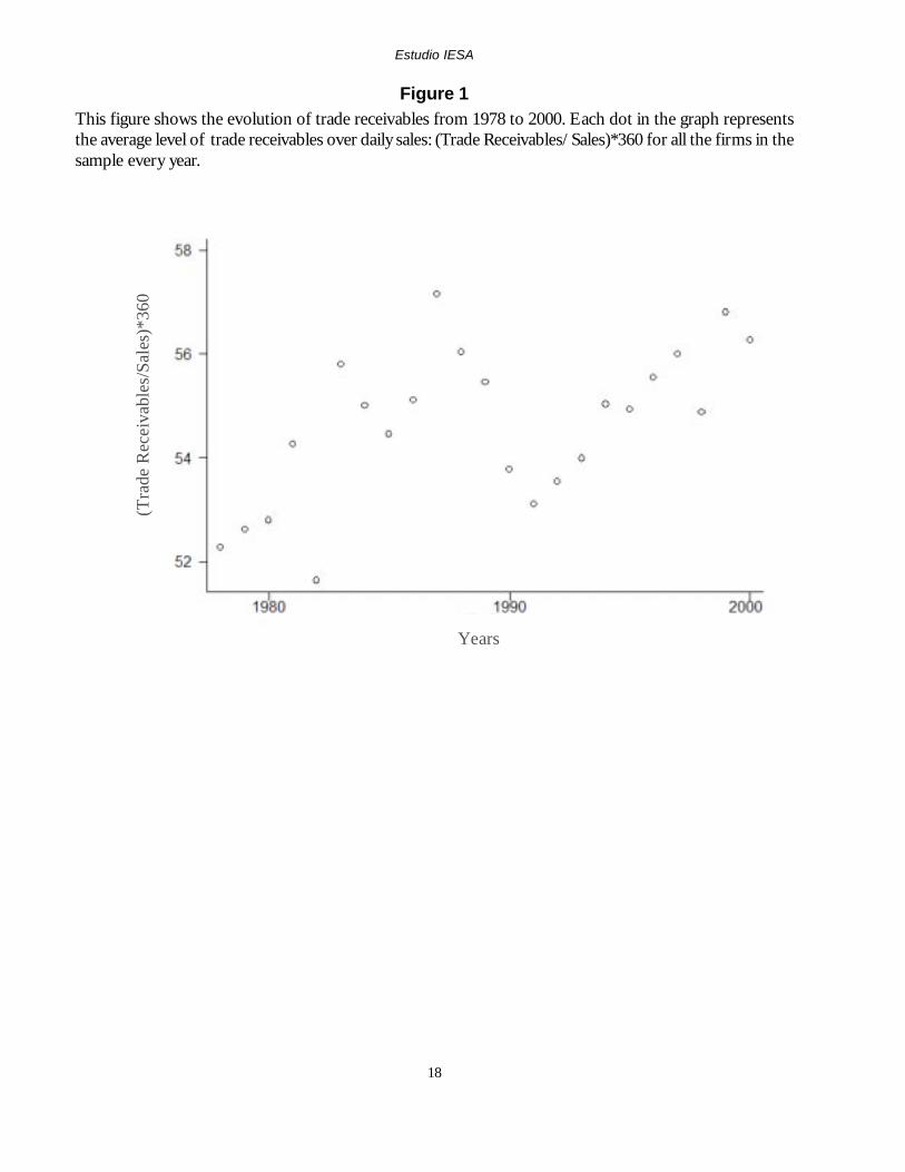
Figure 1 plots the yearly mean of the ratio oftrade receivables to sales (measured in days) forall the firms in the database from 1978 to 2000.Notice that the average number of days that firmsfinance their clients via trade receivables hasgrown, but with a high dispersion around the meanduring the 23 years of data.

The effect of financial distresson trade creditIn this section, we analyze the behavior of tradereceivables of firms when they enter financialdistress and consider the hypothesis that theydecrease their trade receivables, possibly in anattempt to receive their funds more quickly.

We estimate the following equation to study theeffect of financial distress on trade receivables:

(TR/Sales) it = α i + βFDit-1 + γXit + εit [1]

In this model, TR/Sales is the ratio of tradereceivables to sales, measured in days, and definedas: TR/Sales = (Trade Receivables / Net Sales) *3605. FD is a dummy variable equal to one if thefirm is in financial distress in a particular year, andzero otherwise, and X is a matrix of controls.

Given that there is not a widely accepted defi-nition of financial distress, we consider three dif-ferent measures that have been used in the litera-ture. Our first approach is to define financial dis-tress following Asquith, Gertner, and Scharfstein(1994); a firm is in financial distress if its coverageratio (defined as EBITDA/Interest Expenses) is lessthan 1 for two consecutive years or if it is less than0.8 in any given year. Firms that are classified as infinancial distress are identified with a dummy vari-able, i.e., FINDIST.

Although our first measure, FINDIST, is anacceptable definition for financial distress, accord-ing to it, the firm could fail to meet the specifiedcoverage ratio because the interest payments aretoo high, but also because the EBITDA generatedby the firm is too low, i.e., poor economic perfor-mance even if the firm is not excessively lever-aged. To account for this, we also use a second—and seemingly stricter—measure of financial dis-tress that, in addition, takes into account the le-verage of the firm relative to its industry. Morespecifically, we use a dummy variable, FDLEV,equal to one if the firm is (i) highly leveraged and(ii) financially distressed—according to our firstdefinition (i.e., FINDIST=1), and zero otherwise.A firm is considered as highly leveraged when itsleverage is in the top two deciles of its industry inany particular year6.

We follow DeAngelo and DeAngelo (1990) inour third definition of financial distress. We use adummy variable, LOSSFD, equal to one if the firmhas three consecutive years of losses, and zero oth-erwise. This measure is based on the assumptionthat a firm with three consecutive years of losses islikely to behave as a financially distressed firm, evenin the absence of high leverage.

It could be argued that a firm enters financialdistress because its clients fail to pay their bills. Weuse the first lag of the financial distress dummy,i.e., FD, in an attempt to ameliorate any possibleendogeneity problem.

X includes a set of most of the classic controlvariables, which include the firm’s level of tradecredit received from suppliers (i.e., TrPay/CGS), thefirm’s Leverage, the firm’s sales growth (i.e.,DSalest-1), the firm’s level of inventories scaled bytotal assets (i.e., Invent./TA), the firm size and age(i.e., Log(Assets) and Log(Age)), and the firmmarket share (i.e., Mkt_share). We have an addi-

5 This measure has two implicit assumptions: first, it assumesthat all the firms’ sales are made on credit, and second, it as-sumes that sales and trade receivables are not affected by sea-sonality (i.e., sales are homogenously distributed throughout theyear). The inclusion of firm and industry dummies in our mod-els should alleviate any potential problems regarding these as-sumptions.

6 Following Opler and Titman (1994), we measure leverage asthe book value of total debt over book value of debt plus bookvalue of equity. The book value of equity is calculated as TotalAssets - Total Liabilities - Preferred Stocks + Deferred Taxes +Convertible Debt. Other measures of leverage, including onethat considers the market value of equity, do not affect theresults.

Estudio IESA

8

tional control for profitability in the measure offinancial distress, and also use Fama and French(1997) industry dummies and year dummies.

We estimate equation [1] using both pooled OLS

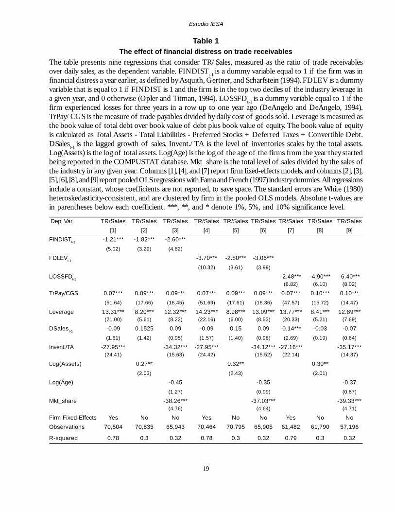
with Fama and French (1997) industry dummiesand fixed-effects models7. The results are in Table1. Columns [1], [2], and [3] show the results usingFINDIST as the measure of financial distress (ourbase-case), the next six columns present robust-ness checks using FDLEV and LOSSFD as mea-sures of financial distress. Columns [1], [4], and [7]use firm fixed-effects estimations, while the othercolumns use pooled OLS models with different setsof control variables. The coefficients for the fi-nancial distress variables are negative and signifi-cant in all cases, showing that firms in financialdistress reduce the level of investment in financ-ing their clients via trade receivables. This result isconsistent with the hypothesis that firms in finan-cial distress underinvest, possibly in an attempt toget cash needed mostly to cope with the financialdistress process. Our findings suggest that the de-crease in trade receivables range between 1 and 6days of net sales8.

In addition, we find a positive effect of TrPay/CGS and leverage on the amount of trade receiv-ables. Firms with higher levels of trade payables tosuppliers or higher levels of debt tend to increasethe level of trade receivables, creating a redistribu-tion channel in the economy, as suggested byMeltzer (1960) in one of the early studies in tradecredit. We also find that larger firms tend to givemore trade receivables to their clients, as alreadyreported by Petersen and Rajan (1997). When weuse market share to control for size of the firm, wefind that firms with higher market share tend to

decrease the level of trade receivables to clients;this is consistent with more powerful firms exercis-ing their market power with their clients. Since afirm’s growth and inventories are also likely to havean effect on the level of trade receivables, we in-clude both as controls in our model.

We argue that the negative effect of financialdistress on trade receivables is due to the urgentneed for cash of financially distressed firms, whichhave a strong reason for decreasing their investmentsin receivables to clients. However, this negative re-lationship could also arise if the distressed firm sellsits trade receivables to a factoring company with-out necessarily reducing the credit to its clients. Tocheck if the use of factoring is what is causing thedrop in receivables, we randomly selected a sampleof forty financially distressed and forty nonfinan-cially distressed firms out of our database, andlooked at their 10-Ks. We found no pattern in theuse of factoring by one or another group of firms,suggesting that factoring should not be causing thedrop in trade receivables9.

A possible concern, given our large datasample, is that macroeconomic factors can affectthe provision of trade credit to clients10. In fact,they may wipe out the differences between firmsin financial distress and healthy ones. First, duringperiods of high inflation, the whole market woulddecrease the level of trade receivables, given thecurrent lower value of receivables. Second, duringperiods of tight monetary policy, we can expect

7 The standard errors in all tables are White’s (1980)heteroskedasticity-consistent, and clustered by firm in the pooledOLS model to allow for an unspecified correlation structurebetween observations of the same firm in different years.

8 If financially distressed firms are also in Chapter 11, and entitledto use debtor-in-possession financing (DIP), they will be morelikely to increase the offer of trade receivables to their clients.The effect of DIP works in a contrary direction to the negativerelationship between financial distress and trade receivables.Therefore, it would only reduce the strength of our results. SeeCarapeto (2003) for a more detailed explanation of DIP.

9 We are interested in the factoring “without recourse,” in whichthe financial institution that buys the trade receivable takes thecredit risk of the transaction. In the case of factoring “withrecourse,” the firm sells the receivables to a financial institutionthat collects the money from the original debtor when the creditis due. If the original debtor fails to pay, then the financial insti-tution can ask the firm to pay. The firm will then keep the tradereceivables in the balance sheet (it does not drop) as a short-term asset, add a debt with the financial institution, and in-crease its cash stock. Unfortunately, there is no data on thetype of factoring that firms are using, but in any case, factoring“with recourse” will only decrease the power of our tests. Seealso Smith and Schnucker (1994) for a more detailed descrip-tion of factoring.

10 Love, Preve and Sarria-Allende (2005) find an important effectof financial crisis on trade credit in emerging economies duringthe nineties.

Estudio IESA

9

trade receivables to be a substitute for financialcredit (Meltzer,1960); consequently the wholemarket should increase the use of trade credit.Consistent with this, Figure 1 shows first a lowerlevel of trade receivables in the high inflation pe-riod of the early eighties, and then a gradual in-crease as the tight monetary policy affects the tradecredit toward the end of the decade.

To check the interaction of macroeconomicconditions and financial distress, we split the samplein four shorter subperiods of time. We group thedata in four time periods (1980-1985, 1986-1989,1990-1995, and 1996-2000) and then estimate equa-tion [1] separately on each subsample. Interestinglyenough, we find that firms in financial distress de-crease their level of trade receivables to clients onlyin the second decade of the sample (i.e., the 1990-2000 period), while the results show insignificantcoefficients in the period 1980-1989. These unre-ported results are consistent with the discussionabove; it is possible that the difference in the useof trade receivables between distressed and healthyfirms is diminished by the fact that macroeconomicfactors equate the use of commercial credit.

The effect of market powerand industry concentrationThe effect of financial distress on trade receivablesdoes not need to be equal for all firms. We haveargued that the ability to negotiate terms of tradecredit with clients might affect the trade receivablespolicies of firms in financial distress. The ability tobargain is a function of the competitive structureof the industry that is usually measured by the firm’smarket power. Depending on the degree of theirmarket power, firms in financial distress that wantto collect their receivables faster might not be ableto do so without affecting the commercial relationwith their clients.

Firms in less competitive or more concentratedindustries should be able to reduce trade receivableswith a lower cost in terms of loss of market share;the higher the market power of the firm, the lower

the probability that a competitor will take its placebased on more generous terms of trade credit. Inaddition, we can expect firms in concentrated in-dustries to have longer-lasting relations with sup-pliers. In the absence of alternative suppliers, cli-ents will be forced to maintain their reputation asreliable customers when suppliers face tough times.

The previous argument can also be comparedwith the model in Klemperer (1987), and is referredto in Chevalier and Scharfstein (1996), which dealwith the importance of switching costs for firms’corporate goals. Switching costs include learningcosts, transaction costs, and costs “artificially” im-posed by firms. Therefore, the customers of a firmface higher switching costs if the industry is con-centrated, which is consistent with the customerspreserving their reputations as clients even if thefirm approaches financial distress.

To address the importance of the industry struc-ture on the ability of the firm to reduce trade re-ceivables when entering financial distress, we repeatthe analysis of the previous section but divide thesample for firms in concentrated and noncon-centrated industries. We use the industry’sHerfindahl Index in each year as our measure ofindustry concentration, and consider an industryto be concentrated if its Herfindahl Index is abovethe median for the year; the rest of the industriesare taken as competitive industries11.

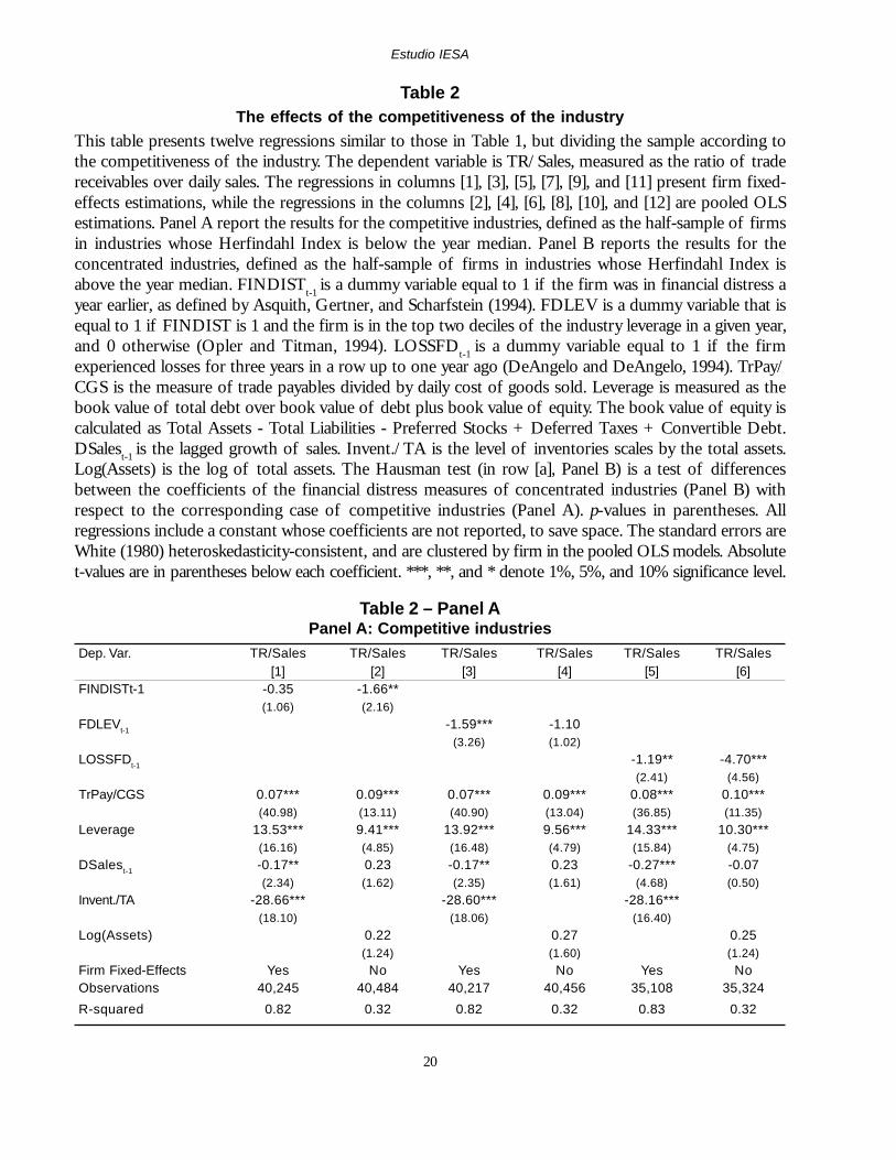
The results are in Table 2. Panels A and B showthe results for competitive and concentrated indus-tries, respectively. Each panel has six columns; thefirst pair of columns show the fixed effects andpooled OLS estimation for the first measure of fi-nancial distress, FINDIST, the third and fourth col-umns repeat the analysis for the second measure,FDLEV, and the last two columns for the thirdmeasure, LOSSFD.

We find that the negative effect of financialdistress on trade receivables is significantly greaterwhen firms are in concentrated industries and have,presumably, more market power. The coefficientson the variables measuring financial distress are

11 The Herfindahl Index is the sum of the squares of the marketshare of the firms in an industry; HFI=?(Mkt_share2).

Estudio IESA

10

negative in all cases; however, they are insignifi-cant in two cases of firms in more competitiveindustries (Panel A). In Panel B of Table 2, wereport a Hausman test of differences between thecoefficients of the financial distress dummies ofconcentrated industries (Panel B) with respect tothe corresponding case of competitive industries(Panel A). In general, we find that the effect offinancial distress on trade receivables is signifi-cantly higher in concentrated industries.

As an additional test, we individually estimateequation [1] on each of the 44 Fama and French(1997) industries to check whether the negativeeffect of financial distress on trade receivables isnegative in all industries. The results (not reported)show that only three industries out of 44 show apositive and significant coefficient for the finan-cial distress dummy. Further investigation on thecharacteristics of these three industries, chemicals(industry number 14), petroleum and natural gas(industry number 30), and transportation (indus-try number 40), show that in most of the years ofthe sample these industries have a Herfindahl In-dex below the median, i.e., they are competitiveindustries, which might explain the trade receiv-ables behavior of financially distressed firms inthese industries.

The results in this section suggest that firmswith enough market power are able to reduce thetrade credit terms to their clients when they are infinancial distress. On the other hand, firms in com-petitive industries that face financial distress andhave a larger probability of going out of businesswill find bill collection more costly, making it harderfor them to reduce their trade receivables.

Profitability problems andcash-flow problemsSo far, we have presented evidence that supportsthe statement that firms reduce their tradereceivables when entering financial distress. Whenfirms enter financial distress they are likely toexperience cash-flow problems, which obliges themto cut the financing extended to their clients if theyhave sufficient market power to do so. However,

firms may behave differently when, prior to enteringfinancial distress, they experience profitabilityproblems.

Petersen and Rajan (1997) find that firms thatexperience losses and sales drops increase theirtrade receivables in an attempt to buy sales vol-ume and market share, or because they are unableto effectively realize the timely repayment of theirreceivables. If the latter occurs, the unwanted in-crease in receivables can be then considered aneffect of financial distress12.

To analyze the behavior of trade receivableswhen firms have profitability problems, we con-struct a model following Petersen and Rajan (1997),and do our estimation using fixed effects in a muchbigger data sample:

TR/Sales it = γi + β1SlsGw_Pit + β2 SlsGw_Nit +

β3NetProfitsit + β4NetLossesit + θXit + εit [2]

In this model, TR/Sales is the ratio of accountreceivables to sales, as defined in the second sec-tion. SlsGw_P is equal to the one-year sales growthif it is positive and to zero otherwise, SlsGw_N isequal to the one-year sales growth if it is negativeand to zero otherwise. NetProfits is equal to thefirm net profits if positive and to zero otherwise.NetLosses is equal to the absolute value of thefirm net losses and to zero otherwise. X is a matrixof control variables. We control for financial dis-tress to distinguish between firms that are only ex-periencing profitability problems (losses) and firmswith cash-flow problems (in financial distress). Wealso control for TrPay/CGS because firms with ahigher level of trade payables will have more fundsto finance their trade receivables13.

12 Petersen and Rajan (1997) use a dataset that covers a crosssection of small firms during the year 1987. This is a year inwhich the average level of TR/Sales was unusually high (seeFigure 1), probably influenced by the stock market crash ofOctober 1987. This is consistent with Meltzer (1960), whostates that during monetary contractions trade credit increases,substituting financial credit.

13 Petersen and Rajan (1997) consider other controls, such asfirm age and maximum available line of credit. Our results donot change if we include a control for age or firm size. Sincewe are using a broader dataset, we do not have information forfirms’ maximum line of credit.

Estudio IESA

11

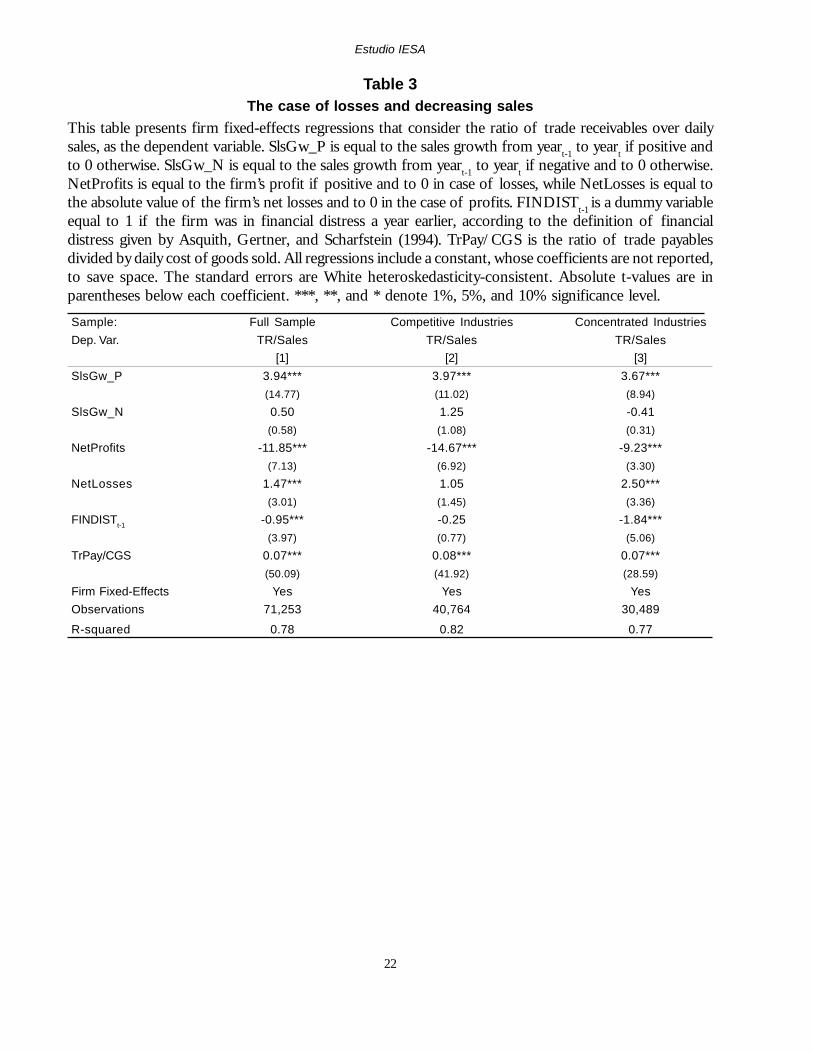
The results are in Table 3. Column [1] showsthe results for the full sample. Consistent withPetersen and Rajan (1997), we find that firms suf-fering losses increase their use of trade receiv-ables14. We also find a positive, although insignifi-cant, effect on trade receivables for firms that ex-perience negative sales growth15. The results onthe controls (FINDISTt-1 and TrPay/CGS) are con-sistent with what we find in the previous sections.

In columns [2] and [3], Table 3, we present theresults separated by industry concentration. Giventhe results in the third section, we also split thesample in this section according to industry con-centration. The results are similar in both cases,except for NetLosses. We find that firms with lossesincrease the trade receivables to their clients byaround two and a half days if they are in concen-trated industries and, presumably, have sufficientmarket power to do so.

These results suggest that when firms with mar-ket power face losses they are able to use tradereceivables in order to “buy” higher sales volumeand market share, consistent with a more domi-nant position with respect to their clients. Firmsin competitive industries do not seem to use tradereceivables as a tool to increase sales volume andmarket share when things start going bad.

The coefficient on FINDISTt-1 confirms theimportance of market power we report in the pre-vious section. It is not distinguishable from zerofor firms in competitive industries and it is nega-tive and significant for firms in concentrated in-dustries. As a robustness check, we also consider(i) market share growth instead of sales growth inequation [2], and (ii) the level of inventories as an

additional control16. The results (not reported) aresimilar.

An alternative interpretation of the results inTable 3 is that when firms experience losses andface negative sales growth, they lose the ability toenforce the payments from their clients, thus theincrease in trade receivables is not wanted by thefirms; it is just a consequence of their financialweakness. That is, firms face higher costs to col-lect their bills when they have problems regardlessof whether they have market power or not. Shouldthis be the case, we would see that when firmsenter financial distress they further increase thelevel of trade receivables, since their ability toenforce the collection of the receivables is furtherweakened by financial distress, and this is not whatwe find in the second section. This reinforces thevalidity of our original interpretation of the resultsin this section.

In addition to the estimation of equation [2],modeled after Petersen and Rajan (1997), we con-sider an alternative test for the hypothesis that firmsincrease their level of trade receivables when theyhave profitability problems before entering finan-cial distress. Specifically, we define a dummy vari-able called NextFD that takes the value of 1 if thefirm is one, two, or three years away from enteringfinancial distress, and 0 otherwise. We then esti-mate a fixed-effects model of trade receivablesover sales (i.e., TR/Sales) on NextFD, FINDISTas a measure of financial distress, and TrPay/CGSas control.

The results are in Table 4. Column [1] showsthe results for the full sample, and columns [2] and[3] for firms in competitive and concentrated in-dustries, respectively. We find that firms that aregoing to enter financial distress in the next one, two,or three years present a higher level of trade receiv-ables; in fact, they give almost two more days of

16 Using market share growth we differentiate a negative salesgrowth due to an industrywide decrease in sales from a firm-specific sales decrease. Using inventories as an additional con-trol, we specifically consider that firms with higher-than-opti-mal level of inventories should try to increase their sales to selloff their excess inventory.

14 Notice that we use the firm losses as a positive number, so apositive coefficient means that an increase in losses (negativeprofits) induce an increase in trade receivables.

15 Petersen and Rajan (1997) find a positive and significant effecton trade receivables for both firms with losses and firms withnegative sales growth. Notice, however, that they do not find asignificant effect of firms with negative sales growth in theirmodel V, where industry dummies and other controls areincluded, as we do in this paper.

Estudio IESA

12

sales in trade receivables to their clients. This ef-fect is robust to firms in both competitive and con-centrated industries (columns [2] and [3]). The re-sults in Table 4 offer stronger support consistentwith the hypothesis that firms increase their useof trade receivables in the years prior to enteringfinancial distress. Consistent with our previous find-ings, the negative effect of financial distress ontrade receivables is stronger for firms in concen-trated industries.

Figure 2 provides additional graphical evidenceof the trade receivables behavior of firms in fi-nancial distress; firms seem to increase their levelof trade receivables to clients in the prefinancialdistress years and then sharply reduce them duringfinancial distress. The timeline of events is in thehorizontal axis and TR/Sales is in the vertical axis.The timeline of events takes the value of 0 in theyear that the firm enters financial distress, and thenadds 1 for each additional year the firm remains infinancial distress. In addition, it takes negative val-ues for all the years in which the firm is not yet infinancial distress, measuring the time (in years) untilthe firm enters financial distress. A horizontal lineis added at TR/Sales=51.46 days, which is theaverage of days of TR/Sales of all the firms inour sample that are not considered in Figure 2, i.e.,that are not in financial distress and will not be infinancial distress during the sample time.

The cost of cutting tradereceivablesIn this section, we estimate the cost of decreasingtrade receivables when in financial distress. First,we look at how much of the drop in the firmperformance is caused by the decrease in the tradereceivables of a firm in financial distress. We thenfollow Opler and Titman’s (1994) logic and checkhow severe the differential cost of financial distressis for firms that decrease their trade receivables.

The cost of cutting trade receivableswhen firms are in financial distressTo estimate the effect of cutting trade receivableswhen firms are in financial distress, we regress

proxies for firm performance on a dummy forfinancial distress, a dummy for significant drops intrade receivables, and their cross effect. The crosseffect of the two dummies (financial distress andsignificant drop in trade receivables) measures themarginal effect of a cut in trade receivables on theperformance of a firm in financial distress.Quantifying this marginal effect allows us toprovide evidence on the cost of financial distresscaused by decreases in the use of trade receivables.

We follow Opler and Titman (1994) in build-ing a model for firm performance:

ittititti

ttititti

XFINDISTSalesDropTRSalesDropTRFINDISTePerformanc

εγβββδ

++

+++=

−−→−

→−−→−

2,1,2,3

2,21,12,

)*)/(()/(

We consider three different proxies for firmperformance ( ttiePerformanc →−2, ) adjusted by in-dustry medians, and use four controls ( 2, −tiX ). Firmperformance is measured over a two-year period,from t-2 to t. The controls are measured at t-2.

To measure financial distress, we considerAsquith, Gertner, and Scharfstein’s (1994) defini-tion and use the first lag (at t-1) of the FINDISTdummy. We measure financial distress at t-1 to as-sure that the firm is in financial distress when welook at its performance. According to this timeline,a firm that is in distress will exhibit a negative per-formance.

We measure a decrease in the use of trade re-ceivables by creating a dummy equal to one if thefirm exhibits a significant drop in trade receivables,normalized by sales and measured in days( ttiSalesDropTR →−2,)/( ).We consider a significantdrop to be when the firm decreases its use of tradereceivables by a larger amount than the 10th per-centile in the entire sample. Alternatively, and as arobustness check, we take into account the 25th

percentile. Since we can expect different drops forfirms in different industries, we also calculate the10th and 25th percentiles by industry, instead ofusing the entire sample. To be consistent with thetiming of the other variables, we measure the dropin trade receivables in the same two-year period aswe use for the firm performance, from t-2 to t.

[3]

Estudio IESA

13

The results are in Table 5. Note that we havefewer observations in these regressions because,following Opler and Titman (1994), we limit our-selves to industries with at least four firms in or-der to carry the industry adjustments. We also dropfirms with sales growth, operating income growth,or equity returns in excess of 200%, and with as-sets lower than $10 million, and sales lower than $5million. In addition we lose one year of data be-cause we need two lags for the models in these re-gressions.

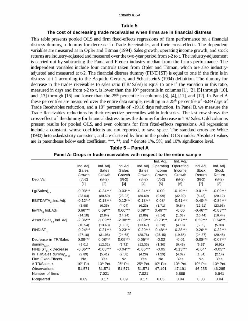
The regressions in Panel A consider high dropsin trade receivables using the entire sample; that iswhen the days of trade receivables drop by morethan -19.16 days (10th percentile), and by more than-6.89 days (25th percentile). In Panel B, we mea-sure the trade receivables reductions by their re-spective percentiles within industries. Odd columnspresent results for pooled OLS regressions andeven columns for fixed-effects regressions. The co-efficient of interest is the cross-effect in the lastrow of each panel. We find that firms in distressexperience drops in performance (the coefficientson FINDIST are negative and significant in all thecolumns of Panel A), but this drop is significantlylarger when there is an important drop in trade re-ceivables, as stated by the negative and significantcoefficients in the interaction term. This result issolid when performance is measured as salesgrowth, but is consistent when using differentmeasures of performance. The results are also solidin relation to different alternatives of measuringthe significance of the drop in trade receivables.

It can be argued that there is a possible endog-enous relation between performance and trade re-ceivables. In other words, if firm performance (salesgrowth) drops, then trade receivables generated bysales should also automatically drop. However, wemeasure trade receivables by sales, which mitigatesthe potential endogeneity problem by consideringdrops of trade receivables with respect to sales asopposed to absolute drops in trade receivables.

The magnitude of the effect of a drop in tradereceivables on firm performance is economicallyimportant. A firm that experiences financial distresswill have a drop in sales of 20-24%, but if this firm

[4]

also decreases its trade receivables by an amountlarger than the 10th percentile of the sample (19days if the entire sample is considered), the dropin sales is an additional 7%. If the drop in tradereceivables is lower (7 days or the 25th percentile),the additional decrease in sales is 4%. These num-bers are similar when we measure performance withthe equity stock returns and somewhat higher whenwe use the growth in operating income as a mea-sure of performance. In this last case, we observean additional drop of 14% in operating incomebecause of a drop in trade receivables.

These results compare well with Opler andTitman (1994). They find that the effect of finan-cial distress on performance amounts to drops of26.4% in sales, and 26.5% in stock returns. Theyconsider that a firm is in financial distress if itsleverage is in the top decile. We find that a firmthat is in financial distress and decreases its tradereceivables will show a total drop in sales and stockreturns of 25-30%. Our results suggest that aboutone-fifth of this drop in performance is due to thedecrease in trade receivables, which supports theassertion of the importance of trade receivablesmanagement by firms in financial trouble.

The effect of cutting trade receivablesfor highly leveraged firms in distressedindustriesWe now complement the previous analysis byfollowing the methodology in Opler and Titman(1994), who investigate the effect of an industrydownturn for highly leveraged firms. We argue thatfirms that decrease their use of trade receivablesin periods of economic distress should lose moresales than firms that do not decrease their use oftrade receivables. In Table 6, we present the samemodel of performance as Opler and Titman (1994)in their Table V:

ittititti

ttititti

XLevHighDistIndDistIndLevHighePerformancεγβ

ββδ++−

++−+=

−−→−

→−−→−

2,3,2,3

2,23,12,

)*)(()(

3, −− tiLevHigh is a dummy for high leverage,equal to one if the firm is in the top three deciles(8-10) of leverage in its industry in any given year,and 0 otherwise. ttiDistInd →−2,)( is a dummy for

Estudio IESA

14

distressed industry, equal to one if the Fama andFrench (1997) industry experiences a negative me-dian sales growth and a median stock return be-low -30%, and it is measured over the same periodthat we measure performance, from t-2 to t.

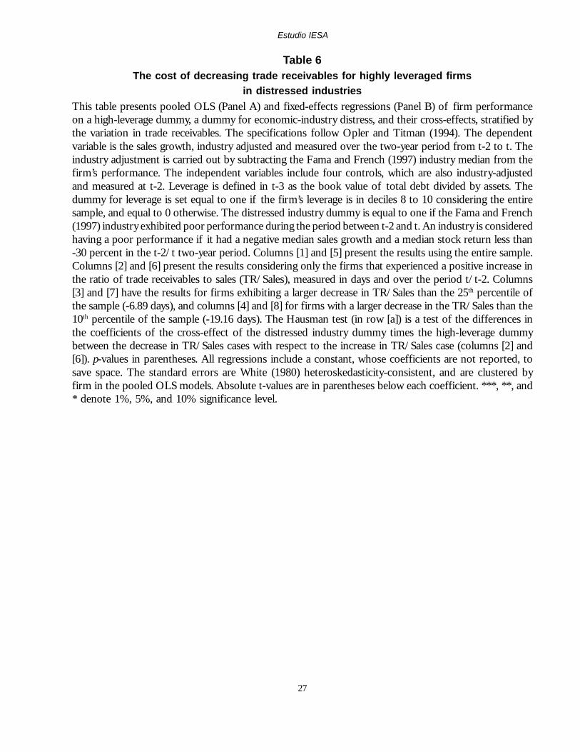
We show the results in Table 6 only for indus-try-adjusted growth in sales17. Columns [1] and [5]present the results using the entire sample. Columns[2] and [6] present the results considering only thefirms that do not decrease trade receivables. Col-umns [3] and [7] show the results for firms with alarger decrease in TR/Sales than the 25th percen-tile of the sample (-6.89 days), and columns [4] and[8] for firms with a larger decrease in TR/Sales thanthe 10th percentile of the sample (-19.16 days). TheHausman test (in row [a]) measures the differencesin the coefficients of the cross-effect of the dis-tressed industry dummy times the high-leveragedummy between the cases of TR/Sales decreasewith respect to the case of non-decrease in TR/Sales (columns [2] and [6]).

Our purpose here is to compare the effect of adecrease in trade receivables on performance forfirms in economic distress. As the Hausman testsin row [a] show, highly leveraged firms that decreasetheir use of trade receivables in situations of eco-nomic distress experience a decline in sales of upto -28% compared with a non-significant decreaseof -1 to -2% when firms do not decrease their tradereceivables. As in Opler and Titman, we control forseveral performance determinants, and include firmfixed effects to proxy for unobservable heteroge-neity.

Compared with Opler and Titman (1994), ourresults using the entire sample are consistent butweaker; the cross-effect of high leverage and dis-tressed industry is negative but insignificant. Thedifference may be explained by the use of a muchlarger sample that includes 22 years of data andsmaller firms. If we use a sample period up to 1991,as Opler and Titman do, and restrict the sample to

firms with assets of more than $50 million, ourresults are practically the same as theirs.

This section presents confirming evidence thatsupports the contention about the importance oftrade receivable management when firms are introuble. We find, first, that decreases in trade re-ceivables account for as much as one-fifth of thedrop in sales and stock returns of firms in financialdistress, and second, that highly leveraged firmsin situations of economic distress experience a sig-nificantly higher drop in sales if they cut their tradereceivables.

Concluding remarksIn this paper, we study the effects of financialdistress on trade receivables, and estimate the costof financial distress due to the inefficientinvestment in trade receivables. It constitutes thefirst attempt to understand the trade receivablespolicy of firms undergoing difficulties and infinancial distress, and the effect of cutting creditof the firm’s clients on the cost of financial distress.

We find that firms increase their level of tradereceivables, presumably to buy market share, whenthey have profitability problems and in the yearsprevious to entering financial distress, but changetheir policy when they are in financial distress, ef-fectively reducing their level of trade receivables.

These results stand up under different defini-tions of financial distress, and on applying a stricterdefinition of distress, they likewise prove to bedurable. Additionally, our results suggest that firmsin concentrated industries have sufficient marketpower to enforce a term reduction in trade receiv-ables when they are in distress. On the other hand,we find that financially distressed firms in com-petitive industries find it difficult to reduce theirtrade receivables. These firms find bill collectionmore costly because their clients may not need tomaintain their reputation as reliable customerssince the probability that their suppliers will go outof business is high and because of the availabilityof alternative providers.17 The results for other measures of performance are similar (not

reported).

Estudio IESA

15

This paper also presents evidence of the im-portance of trade receivables policies for firms infinancial distress. We find, first, that drops in tradereceivables account for as much as one-fifth ofthe average drop in sales and stock returns experi-enced by firms in financial distress, and second,that highly leveraged firms in situations of eco-nomic distress experience a significantly higherdrop in sales if they cut their trade receivables thanif they do not. These results add to the explana-tion of the cost of financial distress reported inthe literature.

The analysis of the trade receivables policy ofdistressed firms and its significant impact on thecost of financial distress that we present in thispaper poses a new set of questions, which war-rants additional research. For instance, what is theimpact of having lower than optimal inventorieswhen firms face financial trouble? Does the man-agement of the firm’s current assets have an im-portant role in reducing the cost of financial dis-tress when the firm faces tough times? These areareas for future exploration.

Estudio IESA

16

ReferencesAlmazan, Andres and Carlos A. Molina (2005): “Intra-industry capital structure dispersion.” Journal ofEconomics and Management Strategy, 14, 263-297.

Altman, Edward (1984): “A further investigation on the bankruptcy cost question.” Journal of Finance,39, 1067-1089.

Andrade, Gregor and Steven Kaplan (1998): “How costly is financial (not economic) distress? Evidencefrom highly leveraged transactions that became distressed.” Journal of Finance, 53, 1443-1493.

Asquith, Paul, Robert Gertner and David Scharfstein (1994): “Anatomy of financial distress: an examinationof junk-bond issuers.” Quarterly Journal of Economics, 109, 625-658.

Carapeto, Maria (2003): “Does debtor-in-possession financing add value?.” Working Paper Cass BusinessSchool.

Chevallier, Judith A. and David S. Scharfstein (1996): “Capital market imperfections and countercyclicalmarkups: theory and evidence.” American Economic Review, 86, 703-725.

Deloof, Marc (2003): “Does working capital management affect profitability of Belgian firms?” Journal ofBusiness, Finance & Accounting, 30, 573-587.

DeAngelo, Harry and Linda DeAngelo (1990): “Dividend policy and financial distress: an empiricalinvestigation of troubled NYSE firms.” Journal of Finance, 45, 1415-1431.

Fama, Eugene F. and Kenneth R. French (1997): “Industry cost of equity.” Journal of Financial Economics,43, 153-193.

Hadi, Ali S. (1992): “Identifying multiple outliers in multivariate data.” Journal of the Royal StatisticalSociety, Series B 54, 761-771.

Hadi, Ali S. (1994): “A modification of a method for the detection of outliers in multivariate samples.”Journal of the Royal Statistical Society, Series B 56, 393-396.

Klemperer, Paul (1987): “Markets with consumer switching costs.” The Quarterly Journal of Economics,102, 375-394.

Leibenstein, Harvey (1966): “Allocative efficiency versus X-efficiency.” American Economic Review, 56,392-415.

Love, Inessa, Lorenzo A. Preve and Virginia Sarria Allende (2005): “Trade credit and bank credit: evidencefrom recent financial crises.” Journal of Financial Economics, forthcoming.

Meltzer, Allan (1960): “Mercantile credit, monetary policy and the size of the firms.” Review of Economicsand Statistics, 42, 429-437.

Mian, Shehzad L. and Clifford W. Smith Jr. (1992): “Accounts receivable management policy: theory andevidence.” Journal of Finance, 47, 169-200.

Estudio IESA

17

Molina, Carlos A. (2005): “Are firms underleveraged? An examination of the effect of leverage on defaultprobabilities.” Journal of Finance, 60, 1427-1459.

Myers, Stewart C. (1977): “Determinants of corporate borrowing.” Journal of Financial Economics, 5, 147-175.

Opler, Tim C. and Sheridan Titman (1994): “Financial distress and corporate performance.” Journal ofFinance, 49, 1015-1040.

Petersen, Mitchell A. and Raghuram G. Rajan (1997): “Trade credit: theories and evidence.” Review ofFinancial Studies, 10, 661-691.

Schmalensee, Richard (1989): “Intra-industry profitability differences in US manufacturing 1953-1983.”Journal of Industrial Economics, 37, 337-357.

Smith, Janet K. and Christijahn Schnucker (1994): “An empirical examination of organizational structure:the economics of the factoring decision.” Journal of Corporate Finance, 119-138.

Titman, Sheridan (1984): “The effect of capital structure on a firm’s liquidation decision.” Journal of FinancialEconomics, 13, 137-151.

White, Halbert (1980): “A heteroskedasticity-consistent covariance matrix estimator and a direct test forheteroskedasticity.” Econometrica, 48, 817-830.

Estudio IESA

18

Figure 1This figure shows the evolution of trade receivables from 1978 to 2000. Each dot in the graph representsthe average level of trade receivables over daily sales: (Trade Receivables/Sales)*360 for all the firms in thesample every year.

(Tra

de R

ecei

vabl

es/S

ales

)*36

0

Years

(Tra

de R

ecei

vabl

es/S

ales

)*36

0

Years

Estudio IESA

19

Table 1The effect of financial distress on trade receivables

The table presents nine regressions that consider TR/Sales, measured as the ratio of trade receivablesover daily sales, as the dependent variable. FINDISTt-1 is a dummy variable equal to 1 if the firm was infinancial distress a year earlier, as defined by Asquith, Gertner, and Scharfstein (1994). FDLEV is a dummyvariable that is equal to 1 if FINDIST is 1 and the firm is in the top two deciles of the industry leverage ina given year, and 0 otherwise (Opler and Titman, 1994). LOSSFDt-1 is a dummy variable equal to 1 if thefirm experienced losses for three years in a row up to one year ago (DeAngelo and DeAngelo, 1994).TrPay/CGS is the measure of trade payables divided by daily cost of goods sold. Leverage is measured asthe book value of total debt over book value of debt plus book value of equity. The book value of equityis calculated as Total Assets - Total Liabilities - Preferred Stocks + Deferred Taxes + Convertible Debt.DSalest-1 is the lagged growth of sales. Invent./TA is the level of inventories scales by the total assets.Log(Assets) is the log of total assets. Log(Age) is the log of the age of the firms from the year they startedbeing reported in the COMPUSTAT database. Mkt_share is the total level of sales divided by the sales ofthe industry in any given year. Columns [1], [4], and [7] report firm fixed-effects models, and columns [2], [3],[5], [6], [8], and [9] report pooled OLS regressions with Fama and French (1997) industry dummies. All regressionsinclude a constant, whose coefficients are not reported, to save space. The standard errors are White (1980)heteroskedasticity-consistent, and are clustered by firm in the pooled OLS models. Absolute t-values arein parentheses below each coefficient. ***, **, and * denote 1%, 5%, and 10% significance level.

Dep. Var. TR/Sales TR/Sales TR/Sales TR/Sales TR/Sales TR/Sales TR/Sales TR/Sales TR/Sales[1] [2] [3] [4] [5] [6] [7] [8] [9]

FINDISTt-1 -1.21*** -1.82*** -2.60*** (5.02) (3.29) (4.82)

FDLEVt-1 -3.70*** -2.80*** -3.06***(10.32) (3.61) (3.99)

LOSSFDt-1 -2.48*** -4.90*** -6.40***(6.82) (6.10) (8.02)

TrPay/CGS 0.07*** 0.09*** 0.09*** 0.07*** 0.09*** 0.09*** 0.07*** 0.10*** 0.10***(51.64) (17.66) (16.45) (51.69) (17.61) (16.36) (47.57) (15.72) (14.47)

Leverage 13.31*** 8.20*** 12.32*** 14.23*** 8.98*** 13.09*** 13.77*** 8.41*** 12.89***(21.00) (5.61) (8.22) (22.16) (6.00) (8.53) (20.33) (5.21) (7.69)

DSalest-1 -0.09 0.1525 0.09 -0.09 0.15 0.09 -0.14*** -0.03 -0.07(1.61) (1.42) (0.95) (1.57) (1.40) (0.98) (2.69) (0.19) (0.64)

Invent./TA -27.95*** -34.32*** -27.95*** -34.12*** -27.16*** -35.17***(24.41) (15.63) (24.42) (15.52) (22.14) (14.37)

Log(Assets) 0.27** 0.32** 0.30**(2.03) (2.43) (2.01)

Log(Age) -0.45 -0.35 -0.37(1.27) (0.99) (0.87)

Mkt_share -38.26*** -37.03*** -39.33***(4.76) (4.64) (4.71)

Firm Fixed-Effects Yes No No Yes No No Yes No NoObservations 70,504 70,835 65,943 70,464 70,795 65,905 61,482 61,790 57,196

R-squared 0.78 0.3 0.32 0.78 0.3 0.32 0.79 0.3 0.32

Estudio IESA

20

Table 2The effects of the competitiveness of the industry

This table presents twelve regressions similar to those in Table 1, but dividing the sample according tothe competitiveness of the industry. The dependent variable is TR/Sales, measured as the ratio of tradereceivables over daily sales. The regressions in columns [1], [3], [5], [7], [9], and [11] present firm fixed-effects estimations, while the regressions in the columns [2], [4], [6], [8], [10], and [12] are pooled OLSestimations. Panel A report the results for the competitive industries, defined as the half-sample of firmsin industries whose Herfindahl Index is below the year median. Panel B reports the results for theconcentrated industries, defined as the half-sample of firms in industries whose Herfindahl Index isabove the year median. FINDISTt-1 is a dummy variable equal to 1 if the firm was in financial distress ayear earlier, as defined by Asquith, Gertner, and Scharfstein (1994). FDLEV is a dummy variable that isequal to 1 if FINDIST is 1 and the firm is in the top two deciles of the industry leverage in a given year,and 0 otherwise (Opler and Titman, 1994). LOSSFDt-1 is a dummy variable equal to 1 if the firmexperienced losses for three years in a row up to one year ago (DeAngelo and DeAngelo, 1994). TrPay/CGS is the measure of trade payables divided by daily cost of goods sold. Leverage is measured as thebook value of total debt over book value of debt plus book value of equity. The book value of equity iscalculated as Total Assets - Total Liabilities - Preferred Stocks + Deferred Taxes + Convertible Debt.DSalest-1 is the lagged growth of sales. Invent./TA is the level of inventories scales by the total assets.Log(Assets) is the log of total assets. The Hausman test (in row [a], Panel B) is a test of differencesbetween the coefficients of the financial distress measures of concentrated industries (Panel B) withrespect to the corresponding case of competitive industries (Panel A). p-values in parentheses. Allregressions include a constant whose coefficients are not reported, to save space. The standard errors areWhite (1980) heteroskedasticity-consistent, and are clustered by firm in the pooled OLS models. Absolutet-values are in parentheses below each coefficient. ***, **, and * denote 1%, 5%, and 10% significance level.

Table 2 – Panel APanel A: Competitive industries

Dep. Var. TR/Sales TR/Sales TR/Sales TR/Sales TR/Sales TR/Sales [1] [2] [3] [4] [5] [6]FINDISTt-1 -0.35 -1.66**

(1.06) (2.16)FDLEVt-1 -1.59*** -1.10

(3.26) (1.02)LOSSFDt-1 -1.19** -4.70***

(2.41) (4.56)TrPay/CGS 0.07*** 0.09*** 0.07*** 0.09*** 0.08*** 0.10***

(40.98) (13.11) (40.90) (13.04) (36.85) (11.35)Leverage 13.53*** 9.41*** 13.92*** 9.56*** 14.33*** 10.30***

(16.16) (4.85) (16.48) (4.79) (15.84) (4.75)DSalest-1 -0.17** 0.23 -0.17** 0.23 -0.27*** -0.07

(2.34) (1.62) (2.35) (1.61) (4.68) (0.50)Invent./TA -28.66*** -28.60*** -28.16***

(18.10) (18.06) (16.40)Log(Assets) 0.22 0.27 0.25 (1.24) (1.60) (1.24)Firm Fixed-Effects Yes No Yes No Yes NoObservations 40,245 40,484 40,217 40,456 35,108 35,324R-squared 0.82 0.32 0.82 0.32 0.83 0.32

Estudio IESA

21

Table 2 – Panel BPanel B: Concentrated industries

Dep. Var. TR/Sales TR/Sales TR/Sales TR/Sales TR/Sales TR/Sales [7] [8] [9] [10] [11] [12]FINDISTt-1 -2.30*** -2.16***

(6.30) (3.01)

FDLEVt-1 -5.44*** -4.66***(10.03) (4.58)

LOSSFDt-1 -3.71*** -5.18***(6.64) (4.61)

TrPay/CGS 0.07*** 0.10*** 0.07*** 0.10*** 0.07*** 0.10***(31.44) (14.32) (31.69) (14.38) (27.43) (12.37)

Leverage 14.27*** 6.94*** 15.60*** 8.53*** 15.14*** 6.41***(13.88) (3.49) (14.98) (4.21) (13.93) (2.95)

∆Salest-1 0.01 -0.02 0.02 -0.03 -0.06 0.08(0.09) (0.12) (0.16) (0.15) (0.53) (0.33)

Invent./TA -27.82*** -27.96*** -27.34***(16.08) (16.18) (14.85)

Log(Assets) 0.32* 0.35** 0.33* (1.79) (2.05) (1.76)

Hausman Test [a] 111.18*** 4.68** 266.19*** 212.65*** 100.55*** 2.49 (p-value) (0.00) (0.03) (0.00) (0.00) (0.00) (0.11)Firm Fixed-Effects Yes No Yes No Yes NoObservations 30,259 30,351 30,247 30,339 26,374 26,466

R-squared 0.77 0.25 0.77 0.25 0.79 0.25

Estudio IESA

22

Table 3The case of losses and decreasing sales

This table presents firm fixed-effects regressions that consider the ratio of trade receivables over dailysales, as the dependent variable. SlsGw_P is equal to the sales growth from yeart-1 to yeart if positive andto 0 otherwise. SlsGw_N is equal to the sales growth from yeart-1 to yeart if negative and to 0 otherwise.NetProfits is equal to the firm’s profit if positive and to 0 in case of losses, while NetLosses is equal tothe absolute value of the firm’s net losses and to 0 in the case of profits. FINDISTt-1 is a dummy variableequal to 1 if the firm was in financial distress a year earlier, according to the definition of financialdistress given by Asquith, Gertner, and Scharfstein (1994). TrPay/CGS is the ratio of trade payablesdivided by daily cost of goods sold. All regressions include a constant, whose coefficients are not reported,to save space. The standard errors are White heteroskedasticity-consistent. Absolute t-values are inparentheses below each coefficient. ***, **, and * denote 1%, 5%, and 10% significance level.Sample: Full Sample Competitive Industries Concentrated IndustriesDep. Var. TR/Sales TR/Sales TR/Sales [1] [2] [3]SlsGw_P 3.94*** 3.97*** 3.67*** (14.77) (11.02) (8.94)

SlsGw_N 0.50 1.25 -0.41 (0.58) (1.08) (0.31)

NetProfits -11.85*** -14.67*** -9.23*** (7.13) (6.92) (3.30)

NetLosses 1.47*** 1.05 2.50*** (3.01) (1.45) (3.36)

FINDISTt-1 -0.95*** -0.25 -1.84*** (3.97) (0.77) (5.06)

TrPay/CGS 0.07*** 0.08*** 0.07*** (50.09) (41.92) (28.59)

Firm Fixed-Effects Yes Yes YesObservations 71,253 40,764 30,489

R-squared 0.78 0.82 0.77

Estudio IESA

23

Table 4Analyzing firms that will enter financial distress

The table presents three firm fixed-effects regressions with respect to TR/Sales, measured as the ratio oftrade receivables over daily sales, as the dependent variable. NextFD is a dummy variable that identifiesfirms that will enter in financial distress in the next one, two or three years. FINDISTt-1 is a dummyvariable equal to 1 if the firm was in financial distress a year earlier, as defined by Asquith, Gertner, andScharfstein (1994). TrPay/CGS is the ratio of trade payables divided by daily cost of goods sold. Allregressions include a constant, whose coefficients are not reported, to save space. The standard errorsare White (1980) heteroskedasticity-consistent. Absolute t-values are in parentheses below eachcoefficient. ***, **, and * denote 1%, 5%, and 10% significance level.Sample: Full Sample Competitive Industries Concentrated IndustriesDep. Var. TR/Sales TR/Sales TR/Sales [1] [2] [3]NextFD 1.85*** 1.58*** 1.85*** (7.90) (5.08) (5.10)

FINDISTt-1 -0.23 -0.61* -1.38*** (0.96) (1.84) (3.76)

TrPay/CGS 0.06*** 0.06*** 0.07*** (51.19) (40.94) (30.28)

Firm Fixed-Effects Yes Yes YesObservations 73,058 41,663 31,395

R-squared 0.77 0.81 0.76

Estudio IESA

24

Figure 2This figure shows the average days of trade receivables for firms that will enter financial distress at somepoint during the sample time. The horizontal axis measures the timeline of the financial distress event. Itis set to 0 the year the firm enters financial distress under the Asquith, Gertner, and Scharfstein’s (1994)definition (FINDIST). Negative values represent the number of years before financial distress, and positivevalues represent the time that the firm has spent in financial distress. The vertical axis measures thenumber of days of trade receivables measured by TR/Sales = (Trade Receivables/Sales)*360. Eachpoint in the graph represents the average number of days of trade receivables that firms show at eachyear. The vertical line drawn at Timeline = 0 shows the moment in which the firms enter in financialdistress and the horizontal line drawn at TR/Sales = 51.46 represents the non-time varying average ofTR/Sales for those firms that are in the sample but do not enter financial distress during the sampleperiod of this study.

Timeline of Financial Distress

(Tra

de R

ecei

vabl

es/S

ales

)*36

0

Timeline of Financial Distress

(Tra

de R

ecei

vabl

es/S

ales

)*36

0

Estudio IESA

25

Table 5The cost of decreasing trade receivables when firms are in financial distress

This table presents pooled OLS and firm fixed-effects regressions of firm performance on a financialdistress dummy, a dummy for decrease in Trade Receivables, and their cross-effects. The dependentvariables are measured as in Opler and Titman (1994). Sales growth, operating income growth, and stockreturns are industry-adjusted and measured over the two-year period from t-2 to t. The industry-adjustmentis carried out by subtracting the Fama and French industry median from the firm’s performance. Theindependent variables include four controls taken from Opler and Titman, which are also industry-adjusted and measured at t-2. The financial distress dummy (FINDIST) is equal to one if the firm is indistress at t-1 according to the Asquith, Gertner, and Scharfstein’s (1994) definition. The dummy fordecrease in the trades receivables to sales ratio (TR/Sales) is equal to one if the variation in this ratio,measured in days and from t-2 to t, is lower than the 10th percentile in columns [1], [2], [5] through [10],and [13] through [16] and lower than the 25th percentile in columns [3], [4], [11], and [12]. In Panel Athese percentiles are measured over the entire data sample, resulting in a 25th percentile of -6.89 days ofTrade Receivables reduction, and a 10th percentile of -19.16 days reduction. In Panel B, we measure theTrade Receivables reductions by their respective percentiles within industries. The last row shows thecross-effect of the dummy for financial distress times the dummy for decrease in TR/Sales. Odd columnspresent results for pooled OLS, and even columns for firm fixed-effects regressions. All regressionsinclude a constant, whose coefficients are not reported, to save space. The standard errors are White(1980) heteroskedasticity-consistent, and are clustered by firm in the pooled OLS models. Absolute t-valuesare in parentheses below each coefficient. ***, **, and * denote 1%, 5%, and 10% significance level.

Table 5 – Panel A Panel A: Drops in trade receivables with respect to the entire sample

Ind. Adj. Ind. Adj.Ind. Adj. Ind. Adj. Ind. Adj. Ind. Adj. Operating Operating Ind. Adj. Ind. Adj.Sales Sales Sales Sales Income Income Stock Stock

Growth Growth Growth Growth Growth Growth Return ReturnDep. Var. (t/t-2) (t/t-2) (t/t-2) (t/t-2) (t/t-2) (t/t-2) (t/t-2) (t/t-2)

[1] [2] [3] [4] [5] [6] [7] [8]

Lg(Sales)t-2 -0.03*** -0.24*** -0.03*** -0.24*** 0.00 -0.19*** -0.01*** -0.09***(23.04) (80.50) (23.22) (80.60) (0.99) (32.99) (6.43) (20.12)

EBITDA/TAt-2 Ind. Adj. -0.12*** -0.13*** -0.12*** -0.13*** 0.08* -0.41*** -0.40*** -0.84***(3.98) (6.35) (4.04) (6.23) (1.71) (9.84) (12.91) (23.98)

Inv/TAt-2 Ind. Adj. 0.60*** 0.09*** 0.60*** 0.09*** 0.49*** -0.06 -0.46*** -0.83***(14.18) (2.84) (14.24) (2.89) (8.14) (1.03) (10.44) (16.44)

Asset Salest-2 Ind. Adj. -2.36*** -1.09*** -2.38*** -1.09*** -0.73*** -0.67*** 0.59*** 0.64***(10.54) (13.63) (10.63) (13.67) (3.28) (4.10) (5.85) (5.90)

FINDISTt-1 -0.24*** -0.21*** -0.23*** -0.20*** -0.48*** -0.28*** -0.26*** -0.22***(27.10) (31.96) (24.68) (28.76) (25.45) (19.85) (24.37) (20.45)

Decrease in TR/Sales 0.09*** 0.08*** 0.05*** 0.05*** -0.02 -0.01 -0.08*** -0.07***dummy(t/t-2) (9.01) (12.31) (9.72) (12.33) (1.30) (0.46) (6.85) (6.91)FINDISTt-1 x Decrease -0.06*** -0.08*** -0.04*** -0.05*** -0.05 -0.13*** -0.04* -0.05**in TR/Sales dummy(t/t-2) (2.89) (5.41) (2.58) (4.29) (1.29) (4.02) (1.84) (2.14)Firm Fixed-Effects No Yes No Yes No Yes No Yes∆ TR/Sales < 10th Pct. 10th Pct. 25th Pct. 25th Pct. 10th Pct. 10th Pct. 10th Pct. 10th Pct.Observations 51,571 51,571 51,571 51,571 47,191 47,191 46,285 46,285Number of firms 7,021 7,021 6,888 6,641R-squared 0.09 0.17 0.09 0.17 0.05 0.04 0.03 0.04

Estudio IESA

26

Table 5 – Panel BPanel B: Drops in trade receivables with respect to the industry

Ind. Adj. Ind. Adj.Ind. Adj. Ind. Adj. Ind. Adj. Ind. Adj. Operating Operating Ind. Adj. Ind. Adj.Sales Sales Sales Sales Income Income Stock Stock

Growth Growth Growth Growth Growth Growth Return ReturnDep. Var. (t/t-2) (t/t-2) (t/t-2) (t/t-2) (t/t-2) (t/t-2) (t/t-2) (t/t-2)

[9] [10] [11] [12] [13] [14] [15] [16]

Lg(Sales)t-2 -0.03*** -0.24*** -0.03*** -0.24*** -0.00 -0.19*** -0.01*** -0.09***(23.43) (80.54) (23.28) (80.50) (0.92) (32.98) (6.15) (20.06)

EBITDA/TAt-2 Ind. Adj. -0.12*** -0.13*** -0.12*** -0.13*** 0.08 -0.41*** -0.40*** -0.84***(3.83) (6.34) (3.88) (6.27) (1.64) (9.80) (13.12) (23.92)

Inv/TAt-2 Ind. Adj. 0.60*** 0.09*** 0.60*** 0.09*** 0.49*** -0.06 -0.46*** -0.83***(14.30) (2.84) (14.25) (2.85) (8.12) (1.00) (10.56) (16.46)

Asset Salest-2 Ind. Adj. -2.37*** -1.09*** -2.38*** -1.09*** -0.74*** -0.67*** 0.58*** 0.64***(10.66) (13.71) (10.63) (13.67) (3.31) (4.08) (5.82) (5.94)

FINDISTt-1 -0.24*** -0.21*** -0.23*** -0.21*** -0.47*** -0.27*** -0.26*** -0.22***(26.78) (32.30) (25.03) (29.52) (25.16) (19.72) (24.09) (20.33)

Decrease in TR/Salesdummy(t/t-2) 0.09*** 0.07*** 0.05*** 0.05*** -0.02 0.01 -0.08*** -0.06***

(9.18) (11.84) (10.81) (12.53) (1.46) (0.60) (7.32) (5.90)

FINDISTt-1 x Decrease inTR/Sales dummy(t/t-2) -0.07*** -0.07*** -0.04** -0.04*** -0.10** -0.14*** -0.07*** -0.07***

(3.35) (4.80) (2.19) (3.64) (2.41) (4.58) (3.09) (2.92)

Firm Fixed-Effects No Yes No Yes No Yes No YesD TR/Sales < 10th Pct. 10th Pct. 25th Pct. 25th Pct. 10th Pct. 10th Pct. 10th Pct. 10th Pct.Observations 51,571 51,571 51,571 51,571 47,191 47,191 46,285 46,285Number of firms 7,021 7,021 6,888 6,641R-squared 0.09 0.17 0.09 0.17 0.05 0.04 0.03 0.04

Estudio IESA

27

Table 6The cost of decreasing trade receivables for highly leveraged firms

in distressed industriesThis table presents pooled OLS (Panel A) and fixed-effects regressions (Panel B) of firm performanceon a high-leverage dummy, a dummy for economic-industry distress, and their cross-effects, stratified bythe variation in trade receivables. The specifications follow Opler and Titman (1994). The dependentvariable is the sales growth, industry adjusted and measured over the two-year period from t-2 to t. Theindustry adjustment is carried out by subtracting the Fama and French (1997) industry median from thefirm’s performance. The independent variables include four controls, which are also industry-adjustedand measured at t-2. Leverage is defined in t-3 as the book value of total debt divided by assets. Thedummy for leverage is set equal to one if the firm’s leverage is in deciles 8 to 10 considering the entiresample, and equal to 0 otherwise. The distressed industry dummy is equal to one if the Fama and French(1997) industry exhibited poor performance during the period between t-2 and t. An industry is consideredhaving a poor performance if it had a negative median sales growth and a median stock return less than-30 percent in the t-2/t two-year period. Columns [1] and [5] present the results using the entire sample.Columns [2] and [6] present the results considering only the firms that experienced a positive increase inthe ratio of trade receivables to sales (TR/Sales), measured in days and over the period t/t-2. Columns[3] and [7] have the results for firms exhibiting a larger decrease in TR/Sales than the 25th percentile ofthe sample (-6.89 days), and columns [4] and [8] for firms with a larger decrease in the TR/Sales than the10th percentile of the sample (-19.16 days). The Hausman test (in row [a]) is a test of the differences inthe coefficients of the cross-effect of the distressed industry dummy times the high-leverage dummybetween the decrease in TR/Sales cases with respect to the increase in TR/Sales case (columns [2] and[6]). p-values in parentheses. All regressions include a constant, whose coefficients are not reported, tosave space. The standard errors are White (1980) heteroskedasticity-consistent, and are clustered byfirm in the pooled OLS models. Absolute t-values are in parentheses below each coefficient. ***, **, and* denote 1%, 5%, and 10% significance level.

Estudio IESA

28

Table 6Panel A: Pooled OLS Panel B: Fixed Effects

Whole ∆ TR/Sales ∆ TR/Sales ∆ TR/Sales Whole ∆ TR/Sales ∆ TR/Sales ∆ TR/SalesSample: sample > 0 < 25 pct. < 10 pct. sample > 0 < 25 pct. < 10 pct.Dep. Var. Ind. Adj. Sales Growth (t/t-2)

[1] [2] [3] [4] [5] [6] [7] [8]

Lg(Sales)t-2 -0.03*** -0.03*** -0.03*** -0.04*** -0.24*** -0.22*** -0.30*** -0.38***(21.46) (19.44) (10.82) (7.93) (85.01) (56.06) (35.81) (19.09)

EBITDA/TAt-2 Ind. Adj. 0.08*** 0.11*** 0 -0.04 -0.04* -0.05* -0.02 -0.07(3.05) (3.37) (0.05) (0.60) (1.85) (1.70) (0.39) (0.82)

Inv/TAt-2 Ind. Adj. 0.62*** 0.69*** 0.44*** 0.36*** 0.07** 0.16*** -0.14 -0.17(15.33) (12.91) (5.66) (2.79) (2.37) (3.70) (1.63) (1.00)

Asset Salest-2 Ind. Adj. -2.19*** -2.17*** -2.05*** -1.57*** -1.09*** -1.15*** -0.82*** -0.33(10.27) (7.42) (6.24) (4.14) (14.46) (9.22) (4.69) (1.04)

Leverage deciles 8-10 -0.02*** -0.02*** -0.02** -0.01 -0.04*** -0.04*** -0.05*** -0.06*dummyt-3 (4.16) (2.98) (2.23) (0.72) (8.76) (6.89) (4.24) (1.95)

Distressed Industry 0.06*** 0.03 0.09*** 0.17*** 0.09*** 0.07*** 0.12*** 0.16**dummy(t/t-2) (3.05) (1.21) (2.60) (2.75) (6.12) (3.16) (3.36) (2.20)

Distressed Industry -0.03 -0.01 -0.09 -0.23** -0.03 -0.02 -0.13* -0.28**dummy(t/t-2) x Leverage (0.87) (0.25) (1.38) (2.27) (0.88) (0.40) (1.95) (2.36)

deciles 8-10 dummyt-3

Hausman Test [a] 3.02* 5.97*** 5.23** 5.70** (p-value) (0.08) (0.01) (0.02) (0.02)

Firm Fixed-Effects No No No No Yes Yes Yes YesObservations 56,722 30,665 12,055 4,158 56,722 30,665 12,055 4,158Number of firms 7,406 6,543 4,708 2,425R-squared 0.05 0.06 0.05 0.05 0.14 0.13 0.17 0.19