Trade Uncertainty and Firm Pollution: The Role ofEmission Cap

Haichao Fan† Guangyuan Guo‡ Yu Liu? Huanhuan Wang∗

December 4, 2020

Abstract

How does a reduction in trade policy uncertainty affect firms’ pollution behavior?

Guided by a simple model, we show that the answer to this question depends on

whether an emission cap exists. We find that the reduced uncertainty increases firm

output by comparable magnitudes across the regions, but they reduce firm SO2 emis-

sion intensity and firm total SO2 emissions only in regions with emission caps. The

decline in SO2 emissions is caused by reduced use of fossil fuel and more abatement

equipment. We also find that the reduced uncertainty improves firms’ productivity

when emission caps exist.

Keywords: Trade policy uncertainty, environmental regulation, emission cap, firm

pollution, firm productivity

JEL codes: F18, F64, Q56, Q58

∗We benefit from comments and suggestions from seminar participants at Fudan University. We ac-knowledge financial support from the “Ten Thousand Talents Program (Young Talents)” of China, YouthInnovative Team on Humanities and Social Sciences of Fudan University and the self-supporting project ofInstitute of World Economy at Fudan University. † Fan: Institute of World Economy, School of Economics,Fudan University, Shanghai, China (e-mail: fan haichao@fudan.edu.cn). Research fellow at Shanghai In-stitute of International Finance and Economics, Shanghai, China. ‡ Guo: School of Economics, FudanUniversity, Shanghai, China (e-mail: glidis@163.com). ? Liu: Department of Public Economics, School ofEconomics, Fudan University, Shanghai, China (e-mail: yu liu@fudan.edu.cn). ∗Wang: East China NormalUniversity, Shanghai, China. (e-mail: ahwanghuanhuan@163.com).

1

1 Introduction

Globalization in recent decades has drastically transformed the economic and environ-mental landscapes of the world. Faced with a dilemma about economic prosperity andclean environment, developing countries may intentionally choose weaker environmen-tal regulations to gain more from globalization, which may also become a source of com-parative advantage (Levinson and Taylor, 2008; Hanna, 2010; Broner et al., 2012; Aicheleand Felbermayr, 2015). This institutional inefficacy has all too often been credited as thereason for the deteriorating environment in developing countries (Banerjee et al., 2008;Alpert et al., 2012; Greenstone and Hanna, 2014). Is it possible that economic growth isobtained without sacrificing the environment? In particular, when a stringent environ-mental regulation is adopted, will a country fail to capture the gains from trade opportu-nities? We address these two questions in this study.

In October 2000, the U.S. government granted permanent normal trade relations (PNTR)to China, which became effective upon China’s accession to the WTO at the end of 2001.Prior to the conferral of PNTR, although Chinese exports to the US had been subject tolow tariffs, these tariffs were reviewed by the U.S. congress annually, which adds uncer-tainty to the tariffs faced by Chinese exporters. The conferral of PNTR ended trade policyuncertainty (Pierce and Schott, 2016). Recent studies find that the end of trade uncertaintyhad substantial effects on exports from China to the U.S. as well as internal migration inChina (Pierce and Schott, 2016; Handley and Limao, 2017; Facchini et al., 2019).

We use the reduction in trade policy uncertainty as an exogenous positive shock toChinese firms’ export opportunities. How will the export shock impact Chinese firms’pollution behavior? On the one hand, the reduction in uncertainty incentivizes exportsand production, which increases pollution (a scale effect). On the other hand, the largerproduction scale and higher profits may encourage firms to adopt better and possiblycleaner machines and technology to improve energy efficiency, which reduces pollutionintensity, measured as pollution per unit of output (a technology effect). This technologyeffect that reduces pollution is also documented in the literature (Levinson and Taylor,2008; Broner et al., 2012; Cherniwchan, 2017). What the literature has not yet examinedare the differential effects of trade on firm pollution with different extents of emissioncontrol, modeled in our setting as emission caps faced by firms.

To more thoroughly analyze the effects of trade policy uncertainty reduction on firmpollution, under the condition that firms face emission control, we develop a multi-country model with heterogeneous firms, where firms’ production entails environmentalemissions. In our model, firms make export decisions to maximize profits and face gov-

1

ernment emission control policies as a production constraint. Our model predicts thatwhen firms face an emission cap, reductions in trade policy uncertainty induce firms toproduce more output but emit less pollution. Reductions in uncertainty also induce firmsto use more labor to substitute for fossil fuel and invest more in abatement equipment. Incontrast, when firms face no emission control, although uncertainty reduction increasesfirm production, it no longer reduces firm pollution.

We test the model predictions using data from three sources. The first dataset is theAnnual Survey of Industrial Firms (ASIF), which contains information on firm produc-tion, such as output, employment, capital, and intermediate inputs. Second, we use datafrom the Annual Environmental Survey of Polluting Firms (AESPF), which covers ma-jor pollutants at the plant level. It also includes information on firm abatement equip-ment investment. We focus on variables related to sulfur dioxide (SO2) emissions becausethe emission cap in China mainly imposes constraints on firm SO2 emissions. The thirddataset is transaction-level import and export data from the China General Administra-tion of Customs (CGAC).

Following Erten and Leight (2019) and Facchini et al. (2019), we compute trade pol-icy uncertainty at the prefecture level. As the conferral of PNTR eliminates export policyuncertainty from China to the U.S., firms in prefectures with higher levels of average un-certainty prior to the conferral would experience a greater decline in prefecture averageuncertainty. We use a difference-in-differences (DID) estimator that compares firm outputand SO2 emissions in high- and low-uncertainty prefectures before and after the confer-ral. We find that the reduction in uncertainty significantly increased firm production butreduced SO2 emissions per unit of output (SO2 intensity). We conduct event studies onfirm output and SO2 intensity to justify our identification assumption for our DID esti-mator. The parallel trends show that the effect on output and SO2 intensity starts in 2001.Firms in prefectures with high and low trade policy uncertainty would have followed thesame trends in production and SO2 emissions in the absence of PNTR conferral.

We then explore the heterogeneous effects across regions with different degree of envi-ronmental regulations. In 1998, two-control zones (TCZs) were established by the Chinesegovernment as special regions with more stringent SO2 emission regulations. We presentthe geographic locations of the TCZs in Figure 1. The SO2 emission cap is more strictlyenforced in TCZs than in non-TCZs. The spatial variation in SO2 emissions control allowsus to examine the heterogeneous effects of uncertainty reductions in firm production andSO2 emissions in TCZs and non-TCZs. Consistent with our prediction, we find that thereductions in trade policy uncertainty increase firm output in both TCZs and non-TCZsby comparable magnitudes, but they reduce total firm emissions and emission intensity

2

only in TCZs.What explains the effects of reduced uncertainty on emission intensity for firms in

TCZs? We find that the reduction in uncertainty decreases coal and fuel use, increasesmanual labor, and increases investment in abatement equipment for firms in TCZs. Incontrast, we do not find comparable effects for firms in non-TCZs. In addition, we findthat firms in TCZs improve total factor productivity more as a result of the reduced un-certainty, consistent with the Porter hypothesis which states that a tougher environmentalstandard can make firms more efficient and innovative (Porter and Van der Linde, 1995).1

Our study is related to two strands of literature. First, this paper is closely related tothe emerging literature that uses firm- or plant-level data to examine the impact of tradeon the environment. The current literature primarily focuses on developed countries–inparticular the U.S.–to document that exporters pollute less than non-exporters (Holla-day, 2016; Cui et al., 2016; Forslid et al., 2018). Cherniwchan (2017) further analyzes theimpact of trade liberalization on a firm’s total emissions and emission intensity in the con-text of NAFTA. In a developing country context, Barrows and Ollivier (2016) use Indianfirm-level data to study the effects of an export demand shock on total emissions, out-put, and emission intensity. Gutierrez and Teshima (2018) use Mexican plant-level andsatellite imagery data to examine the impact of import competition generated by outputtariff reductions on plants’ environmental outcomes. Our paper complements these ear-lier studies by focusing on the impact of an export demand shock induced by reducedtrade policy uncertainty on Chinese firms’ total emissions, output and emission intensity.Moreover, we examine the differences in these effects across regions with different de-grees of environmental regulations on pollution emissions. To summarize, our paper isin line with the literature but also differs from it by emphasizing the role of the emissioncontrol.

Second, our paper is also related to studies on trade policy uncertainty. Pierce andSchott (2016) study the effect of a reduction in U.S. trade policy uncertainty on U.S. man-ufacturing firms after China’s accession to the WTO. Handley and Limao (2017) use adynamic general equilibrium model to argue that a reduction in trade policy uncertaintyafter China’s accession to the WTO significantly contributed to the country’s export boomto the United States. Crowley et al. (2018), Garred (2018), and Imbruno (2019) provide em-

1Our findings highlight the joint effects of export opportunity and domestic environmental regulation.When firms face an opportunity to export, and existing domestic environmental regulations constrain pol-lution, firms may adjust production and improve efficiency to increase production scale and export. Thisis consistent with the Porter hypothesis (Porter and Van der Linde, 1995). The positive effects of morestringent environmental regulations on firm productivity are also documented by Acemoglu et al. (2016),Aghion et al. (2016), Gutierrez and Teshima (2018), and Aghion et al. (2020).

3

pirical evidence on how trade policy uncertainty affects exports and imports. Erten andLeight (2019) and Facchini et al. (2019) examine the impacts of the reduction in trade pol-icy uncertainty associated with China’s WTO accession on structural transformation inChina and China’s “Great Migration”, respectively. The focus of our paper is the environ-mental consequences of trade policy uncertainty, which differs from the aforementionedstudies.

The remainder of the paper proceeds as follows. Section 2 introduces environmentalregulations and TCZs in China. Section 3 presents a simple model. Section 4 discusses ourempirical strategy and describes the data and measures. Section 5 reports the empiricalresults. Section 6 concludes the paper.

2 Institutional Background

The traditional method to control industrial pollution in China requires firms’ pollutiondischarge to be below a given concentration value, which specifies the maximum level ofemission intensity (i.e., emissions per unit of output) for each pollutant. Failure to complywith the requirement may trigger fines and penalties. This method, however, ignores thetotal amount of pollution of a firm, which leaves a loophole that results in high levels ofoverall pollution at the firm and regional levels. To close this loophole, China adoptedan emission cap method in 1996 as a part of the 9th Five-year Plan. This method sets anoverall emission target for all major pollutants and has since been the main method forpollution control in China.2

Emission caps are common practice across countries. For example, the U.S. created the“Acid Rain Program” and Japan initiated the “Water-basin COD Emission Target ControlProgram” to combat chemical emissions; there is also of course the worldwide carbonemission reduction agreement under the Kyoto Protocol.3 In contrast to the commoncap-and-trade mechanism, the method in China sets an overall cap but has no tradingmechanism, primarily because China has not yet established institutions to support mar-ket transactions of emission permits.

In practice, the central government first sets a national cap, or emission target and thenallocates targets to each province, and each province then divides the targets among pre-

2The 9th Five-year Plan defined 12 pollutants as “critical pollutants” and requires the total emissions ofeach pollutant in 2000 to be lower than those in 1995. The 10th Five-year Plan further mandated that theemissions of 6 major pollutants be reduced by 10% in 2005 relative to 2000 (see the “National EnvironmentalBureau, Decomposition Plan on Emission Control of Critical Pollutants during the 10th Five-year Plan,2001”).

3See the United Nations Framework Convention on Climate Change.

4

fectures in its jurisdiction for implementation. There are 333 prefectures in total, whichform a government hierarchy in between provinces and counties.4 The target assign-ments at the prefecture level take into account the population, economic size, industrialstructure, past emissions, and environmental quality of each prefecture.5 Each prefecturethen further assigns emission targets to firms; the detailed assignment rules are not madepublic by the government. Guaranteeing emission reductions demands not only care-ful scrutiny and government approval at the factory or establishment level, especially inhigh-pollution industries, but also requirements by the prefecture government that firmsadopt pollution abatement facilities such as desulfurization of coal or gas combustionor to remove sources with high emission intensity and outdated production equipment.The government regularly sends inspectors to monitor and record pollution emissions toenforce its regulation.

In effect, this emission cap method is applied nationwide and implemented throughthe government administrative hierarchy. The amounts of pollution emissions are recordedat the firm level before they are summed up at jurisdictional levels. Statistics are reportedthrough government hierarchies in a bottom-up manner and affirmed by the central gov-ernment. The central government uses these statistics to evaluate officials’ competencyand accountability. This process takes place annually.

Among all pollutants that are regulated by an emission cap in China, SO2 is grantedthe top priority. In January 1998, the central government enacted a “Two-control Zone”policy to identify priority regions to reduce SO2 emissions to prevent acid rain. Prefec-tures with annual average precipitation pH values exceeding nationally mandated thresh-olds are designated as Acid Rain Control Zones: prefectures with annual average SO2emission levels exceeding nationally mandated thresholds are designated as SO2 ControlZones. Following these standards, a total of 175 prefectures were designated as “Two-control Zones” (TCZs) by the central government in 1998. More stringent environmentalregulations on emission caps are thus adopted in these zones. For example, new coalmines producing coal with sulfur content higher than 3% are prohibited, and any suchexisting coal mines are to be shut down. No new thermal power plants combusting coalare to be built near large prefectures. Firms in high-emission-intensity industries includ-ing the petrochemical, metallurgical, architecture material, and nonferrous metal indus-tries are obliged to adopt pollution reduction equipment.6 These requirements are more

4The 333 prefecture-level divisions include 7 prefectures, 293 prefecture-level cities, 30 autonomousprefectures, and 3 leagues. We call all of these types of divisions prefectures for simplicity.

5See the “National Environmental Bureau, Implementing Program on Emission Control of Critical Pol-lutants during the 9th Five-year Plan, 1997.”

6See the “Approval of The Central Government on SO2 Control Zones and Acid Control Zones Plan,

5

stringent in TCZs than those in non-TCZs.Figure 2 plots the annual aggregate GDP and SO2 emissions in TCZs and non-TCZs

between 1999 and 2006. The GDP data are obtained from the CEIC database, and the SO2emission data are collected from the China Statistical Yearbook on Environment, pub-lished by the Ministry of Ecology and Environment of China. We treat 1999 as the bench-mark year (value=100). The figure shows that although GDP had been rising rapidly inboth types of region, the SO2 emissions in TCZs remained relatively stagnant between1999 and 2006, which reveals the relatively more stringent SO2 emission control in TCZs.The difference in the strength of environmental regulation between TCZs and non-TCZshelps us to identify the differential impacts of reduced trade policy uncertainty on firmbehavior with and without an emission cap.

3 Model

In this section, we develop a multi-country trade model with heterogeneous firms wherefirms’ production entails environmental emissions.

3.1 Preferences

A representative consumer in country j has a constant elasticity of substitution (CES)utility function given by:

Uj =

[N

∑i=1

∫ω∈Ωij

[qij (ω)

] σ−1σ dω

] σσ−1

+ Ψ(Ej)

, (1)

where N represents the total number of countries and i is the source country of the prod-uct, ω indexes the product variety in set Ωij available in country j, qij denotes the quantityof variety ω, σ > 1 is the elasticity of substitution between varieties, and Ψ

(Ej)< 0 repre-

sents the negative impact of pollution emission Ej on the individual’s utility.7 Consumeroptimization yields the following the demand function for variety ω in country j:

qij (ω) =[pij (ω)

]−σ Pσ−1j Ij, (2)

1998.”7We assume that Ψ

(Ej)< 0 and Ψ′

(Ej)< 0. That is to say, the impact of pollution emission on

individual’s utility is negative and this negative impact increases in pollution emission Ej.

6

where pij (ω) is the price of variety ω faced by consumers in country j. The aggregate

price index in country j is defined by Pj =[∑N

i=1∫

ω∈Ωijpij (ω)1−σ dω

] 11−σ and Ij is the

total spending in country j.

3.2 Firm behavior

Suppose the firm is in the market of monopolistic competition. Each firm in country iproduces only one kind of heterogeneous product and its productivity is ϕ. Like Melitz(2003), firms in country i need to pay f e

i units of labor in order to acquire a blueprint

and then draw a productivity from a Pareto distribution, i.e., Gi (ϕ) = 1−(

biϕ

)θ, where

θ is the Pareto location parameter and bi represents the productivity of country i. Firmsin country i need to pay a fixed export cost, amounting to fij units of domestic laborwhen exporting to country j. In addition, firms in country i also need to pay a tariff of tij

when exporting to country j. To characterize trade policy uncertainty faced by Chinesefirms exporting to the U.S. prior to PNTR conferral, we assume that the tariff can be seteither at a high non-PNTR value at t1

ij with probability ηij or at a low PNTR value at t2ij

with probability 1 − ηij. The average tariff is therefore tij = ηijt1ij +

(1− ηij

)t2ij, where

0 ≤ ηij ≤ 1.Consider country i to be China. When j = U.S., ηij is above 0 prior to conferral, and it

is equal to 0 after conferral. When j 6= U.S., we assume that ηij remains zero throughoutthe study period. In what follows, we analyze how the tariff change induced by thechange in the probability ηij affects the firm’s production and emission behavior.

Following Shapiro and Walker (2018), we assume that each firm produces two out-puts: an industrial good and emissions. In order to reduce emissions, a fraction of θ ratioof production inputs is used to reduce pollution and the other (1− θ) ratio of productioninputs is used to produce products. The fraction of labor θ spent in reducing pollution isan endogenous choice that ultimately varies with a firm’s productivity. The firm’s pro-duction function is given by the following equation:

qij(ϕ) = (1− θ)ϕlγiij M1−γi

ij , (3)

where lij is the labor demand, Mij is the demand for final material inputs by firms (itsproduction function is the same as utility function). Firms product emissions with thefollowing technology:

eij(ϕ) = (1− θ)1/α ϕlγiij M1−γi

ij , (4)

The firms need to pay the costs including the emission tax, pollution fee and so on. We

7

assume that the pollutant cost per unit of emission is te,i.We proceed by using Equation (3) to solve for (1− θ), and, in turn, be used to sub-

stitute for (1 − θ) in Equation (4). This gives us an integrated expression for the jointproduction of goods and emission, which exploits the fact that although pollution is anoutput, it can equivalently also be treated as an input. Hence, we have:

qij =(

ϕlγiij M1−γi

ij

)1−αeα

ij. (5)

In equation (5), production use labor as well as emissions. The parameter α denoteshow intensive the industry is in the use of labor versus the use of emissions.

3.3 Firm’s behavior

In the first stage, given the wage wi, the pollutant cost per unit of emission te,i and theexport decision Iij, firms solve the following problem:

max ∑j

Iij (ϕ)

[pij(ϕ)qij(ϕ)

τij− wilij(ϕ)− Pi Mij − te,ieij(ϕ)

](6)

where qij(ϕ) =[pij(ϕ)

]−σ Pσ−1j XD

j (7)

qij(ϕ) = (1− θij)ϕlγiij M1−γi

ij (8)

eij(ϕ) = (1− θij)1/α ϕlγi

ij M1−γiij (9)

where XDj is the demand by both consumers and firms,

pij(ϕ)τij

denotes the value obtainedby firms for one unit of export to country j and τij = 1 + tij. The previous problem isequivalent to

maxθij,lij

∑j

Iij (ϕ)

((

1− θij)

ϕlγiij M1−γi

ij

) σ−1σ

τijP

σ−1σ

j I1σj − wilij(ϕ)− Pi Mij − te,i

(1− θij

)1/αϕlγi

ij M1−γiij

(10)

8

Solving this optimization problem by choosing θij, lij and Mij yields,

ασ− 1

σpij(ϕ)qij(ϕ) = τijte,ieij(ϕ) (11)

γiσ− 1

σpij(ϕ)qij(ϕ) = τij

[wilij(ϕ) + γite,ieij(ϕ)

](12)

(1− γi)σ− 1

σpij(ϕ)qij(ϕ) = τij

[Pi Mij + (1− γi) te,ieij(ϕ)

](13)

The previous equations imply the optimal price equal to

pij(ϕ) =σ

σ− 1

τij

(wγ

i P1−γi

)1−αtαe,i

ϕ1−ααα((1− α) γ

γii (1− γi)

1−γi)1−α

(14)

Firms decide on whether or not to sell in country j. The exporting productivity cutoffϕ∗ij is determined by comparing their profit and the fixed exporting cost according to thefollowing equation:

1σ

pij(ϕ∗ij)qij(ϕ∗ij)

τij= fijwi (15)

Hence, the productivity cutoff ϕ∗ij amounts to

ϕ∗ij =

(στij fijwi

ΘijPσ−1j XD

j

) 1(1−α)(σ−1)

(16)

where Θij =

(σ

σ−1τij

(wγ

i P1−γi

)1−αtαe,i

αα((1−α)γγii (1−γi)

1−γi)1−α

)1−σ

.

3.4 Equilibrium

The average productivity of exporting firm from country i to country j, ϕij, is defined as:

ϕij =

∫ ∞

ϕ∗ij

(ϕij)(1−α)(σ−1) g (ϕ)

1− G(

ϕ∗ij

)dϕ

1(1−α)(σ−1)

=

(θ

θ − (1− α) (σ− 1)

) 1(1−α)(σ−1)

ϕ∗ij

(17)Since the average productivity level ϕij is completely determined by the productivitycutoff ϕ∗ij, the average profit and revenue levels from country i to country j are also tied

9

to the cutoff level ϕ∗ij:

πij(

ϕij)=

(1− α) (σ− 1)θ

rij(

ϕij)

σ=

(1− α) (σ− 1)θ − (1− α) (σ− 1)

rij

(ϕ∗ij

)σ

(18)

In the equilibrium with free entry, the expected value for potential entrants should beequal to the fixed entry cost f e

i wi, i.e.,

Ni f ei wi = ∑

jNi

(b

ϕ∗ij

)θ

πij(

ϕij)=

(1− α) (σ− 1)θσ

Yi (19)

where Yi denotes the total output:Yi = ∑j Xij (20)

where Xij denoting the aggregate trade flow from country i to country j, equals to

Xij =Niθσbθ

(τij fijwi

)1− θ(1−α)(σ−1) Θ

θ(1−α)(σ−1)ij τ−1

ij

∑i′ Ni′θσbθ(

τi′ j fi′ jwi′)1− θ

(1−α)(σ−1) Θθ

(1−α)(σ−1)i′ j

XDj (21)

where XDj is the sum of the consumers’ demand Ij and the firms’ demand (1−γj)(1−α)(σ−1)

σ Yj.Consumer’s expenditure Ij satisfies:

Ij = wjLj + te,jEj + ∑i

tijXij (22)

The equation (12) implies that the total emission satisfies:

te,iEi =σ− 1

σα ∑j Xij =

σ− 1σ

αYi (23)

Trade balance condition, which means that the total expenditure amounts to sell revenueplus tariff revenue, implies:

wiLi =

(1− ((1− γi) (1− α) + α) (σ− 1)

σ

)Yi (24)

10

Aggregate price could be rewritten as

Pj =

∑i

Ni

(b

ϕ∗ij

)θ ∫ ∞

ϕ∗ij

pij (ϕ)1−σ g (ϕ)

1− G(

ϕ∗ij

)dϕ

11−σ

(25)

=

∑i

Nibθθ

θ − (1− α) (σ− 1)

(στij fijwi

ΘijXDj

)− θ(1−α)(σ−1) στij fijwi

XDj

−1−α

θ

(26)

Using a method inspired by Dekle, Eaton, and Kortum (2007; 2008), we denote thepost adjustment value of any variable x as x′ and the change in its value as x = x′

x , a hatdenotes the ratio between the counterfactual and factual value. The emission control sys-tem, together with Equations (19), (20), (22), (23), (24) and (26), construct the equilibriumsystem with variables (wi, Ei, te,i, Pi Yi, Ii, Ni). These four equations imply:

Yi = ∑j

λijMij (27)

Ij =wjLj

Ijwj Lj +

te,jEj

Ijte,jEj + ∑

i

tijXij

IjMij (28)

Yi = wiNi (29)

Yi = te,iEi (30)

Yi = wi (31)

Pj =

∑i

ξijNi

(τijw

γ(1−α)i P(1−γ)(1−α)

i tαe,i

)− θ1−α

(τijwi

XDj

)1− θ(1−α)(σ−1)

−(1−α)

θ

(32)

where Mij =Ni(τijwi)

1− θ(1−α)(σ−1)

(τijw

γ(1−α)i P(1−γ)(1−α)

i tαe,i

)− θ1−α τ−1

ij

∑i′ Ni′ ξi′ j

(τi′ jwi′

)1− θ(1−α)(σ−1)

(τi′ jw

γ(1−α)

i′ P(1−γ)(1−α)

i′ tαe,i′)− θ

1−α

XDj , XD

j =Ij

XDj

Ij +(1−γj)(1−α)(σ−1)Yj

σXDj

Yj,

λij =Xij

∑j Xij, ξij =

τijXij∑i τijXij

, XDi = ∑

jXij + ∑

vtviXvi, Ii =

(1− (1−γi)(1−α)(σ−1)

σ

)∑j

Xij +

∑v

tviXvi, Yi = ∑j

Xij, wiLi =(

1− ((1−γi)(1−α)+α)(σ−1)σ

)∑j

Xij, te,iEi = α(σ−1)σ ∑

jXij. Fol-

lowing Hsieh and Ossa (2016), we treat the mean change in all countries’ wage index asthe numeraire. Then, we can use the previous several equations to solve for the changesin variables at general equilibrium in response to a reduction in trade uncertainty, givenbilateral trade data and values of the key parameters.

We assume that only China has adopted emission target control theme. As for countryi except from China, pollution cost te,i in that country is unrelated with trade activities

11

since they wouldn’t adopt emission target control theme. According to Equation (30), wehave Ei = Yi for i 6= China. For China, we set Ei = (1− ρ) Yi + ρκ, where 0 ≤ ρ ≤ 1and 0 < κ ≤ 1. When ρ = 0, there is no emission controls in China. A higher value of ρ

corresponds to more stringent emission control. The value of κ reflects the emission cap.For example, κ = 0.975 means the emission cap is the 97.5 percentage of its initial value.

3.5 Data, Parameters and Results

This section describes how we estimate the parameters in the quantitative analysis, thensimulates the estimated effects of a reduction in trade uncertainty.

The elasticity of substitution σ, the pollution elasticity α and the trade elasticity θ areestimated pursuant to steps suggested by Shapiro and Walker (2018). To be specific, wetake an overall value 0.011 for pollution elasticity α as Shapiro and Walker (2018), imply-ing that firms pay 1.1 percent of their total production costs on pollution taxes. In ac-cordance with Broda and Weinstein (2006) who estimate the product-specific elasticitiesof substitution for 73 counties based on a nested constant-elasticity-substitution utilityfunction, we take the elasticity of substitution σ = 5.8 According to our theory, firms’domestic sales follow a Pareto distribution with a shape parameter θ − (1− α) (σ− 1).Given the estimates of σ and α, we could then back out the trade elasticity θ by regress-ing the logarithm of the rank of firm domestic sales on the logarithm of firm domesticsales, using Chinese firm-level manufacturing survey data from the National Bureau ofStatistics of China (NBSC). The estimated value of θ equals to 4.41.

In order to solve for the equilibrium relative changes, we also need the complete ma-trix consisting of the trade flows Xij and the tariff τij. We first obtain the trade flows atyear 2001 from World Input-Output Database (WIOD), covering 43 countries, and therest of the world. Then, we obtain their bilateral applied tariff data at year 2001 from theWTO-TRAINS database. For U.S., its tariff imposed on imports from China is a functionof non-MFN applied tariff and MFN applied tariff before China’s accession to WTO. AfterChina’s accession to the WTO, it becomes the MFN applied tariff.

The first three panels of Figure 3 describes the impact of a reduction in policy uncer-tainty on output, emission and emission intensity, respectively. The last panel of Figure 3reflects the impact of a reduction in policy uncertainty on 1− θ.9 As shown in Figure 3, re-

8We aggregate their estimates for China and U.S. by taking means, which equal to 6.19 and 4.17 respec-tively. Hence, we take σ = 5, a value in-between.

9Figure 3 corresponds to the case of κ = 0.975. Figures A.1 and A.2 in the Appendix correspond to κ = 1and κ = 0.95. We find similar patterns pertaining to the impact of diminished trade policy uncertaintyamong figures with different values of κ.

12

duction in trade policy uncertainty (i.e., higher probability of setting non-PNTR, η) raisesoutput and pollution emission. When there exists the emission control (i.e., ρ 6= 0), theemission intensity decrease. As to output, diminished trade policy uncertainty increasesoutput by 6%. More stringent environmental regulation only slightly weaken this outputeffect if the probability of setting non-PNTR before China’s accession to WTO equals toone. After comparing two extreme situation when ρ = 0 and ρ = 1, we only find 0.13%less output impact from decreased trade policy uncertainty when incorporating the in-fluence from strict environmental regulation. If the emission cap is lower than its initialbenchmark value (i.e., κ < 1), the emission would turn from increase to decrease after areduction in policy uncertainty. Trade policy uncertainty would not affect the emissionintensity without emission control. It always equals to one. The emission cap reduces theemission intensity due to higher emission costs caused by more stringent environmentalregulation (see Figure 4). Meanwhile, the last panel shows the substitutive relation of in-puts between firms’ production and emission control. Without emission control (ρ = 0),more inputs would be used in production which is indicated by the increase of 1− θ. Withstringent emission control (ρ = 1), more inputs are used in emission reduction which isindicated by the decrease of 1− θ.

4 Empirical Specification, Data, and Measures

In this section, we specify our econometric models and describe the data and measuresthat we use for estimation.

4.1 Empirical specification

In this section, we present our empirical strategy to test our model predictions. Proposi-tion 1 suggests that when an overall emission cap exists, reducing trade policy uncertaintyincreases firm production but reduces firm SO2 emission intensity. We test this predictionby estimating the following regression:

yit = βUncertaintyp × Postt + γXpt + ∑t

θtXi × δt + δt + γi + εit, (33)

where yit denotes firm i’s outcome in year t. Uncertaintyp measures prefecture p’s ex-port policy uncertainty prior to WTO accession. Following Facchini et al. (2019), we useexport-weighted uncertainty at the prefecture level to construct this variable. Postt is adummy variable indicating whether year t is post WTO accession. We control for the in-

13

teractions between year dummies and firm initial output and SO2 emissions, Xi, to allowfirms with different initial outputs and emissions to have different time paths. To allevi-ate biases caused by macroeconomic changes at the prefecture level, we also include thevector of controls Xpt, which includes contemporaneous prefecture-level GDP per capitaand population density. δt and γi are year and firm fixed effects, respectively. Controllingfor year fixed effects ensures that our estimates will not capture effects due to other con-current macroeconomic changes or common time trends, and controlling for firm fixedeffects eliminates any omitted variable bias caused by time-invariant firm characteristics.εit is an error term capturing all unobserved factors that influence yit.

The main parameter of interest in equation (33) is β, which estimates how the changein a firm’s outcome before and after WTO accession differs across firms in prefectures ofdifferent levels of pre-WTO export uncertainty. Our model predicts that, relative to firmslocated in prefectures with low uncertainty, firms in prefectures with high uncertaintyprior to WTO accession increase output more. The overall emission control sets a con-straint on total SO2 emissions and therefore SO2 emission intensity, i.e., per-unit outputSO2 emissions, is expected to decline. The effects on firm SO2 emissions can be ambigu-ous.10 To test these hypotheses, we use the logarithm of a firm’s output, SO2 emissions,or emission intensity of SO2, as the dependent variable in equation (33). We expect β tobe positive, zero (or negative), and negative, respectively, in these regressions.

To further test whether emission control is indeed the key driver of our results, weconduct a triple-difference estimation strategy to see if the policy effects are different forfirms located in TCZs from those in non-TCZs. Firms in TCZs face more stringent SO2emission control. The regression takes the following form:

yit = β0TCZi ×Uncertaintyp × Postt + β1Uncertaintyp × Postt + β1TCZi × Postt

+ γXct + ∑t

θtXi × δt + δt + γi + εit,(34)

where TCZi is a dummy variable that indicates whether firm i is located in a two-controlzone during our study period. We are interested in the estimated coefficient, β0, whichshows the heterogeneous policy effects by firm location. Because firms located in TCZsface more stringent emission control, we expect β0 to be negative for firm SO2 emissionsand SO2 emission intensity. For firm output, the expected sign of β0 is ambiguous. On theone hand, there is a cost effect. Firms located in a TCZ face an emission cap that imposes

10The firm SO2 emission cap may decline for two reasons. First, overall jurisdictional emissions arerequired to decline, especially for the TCZs. Second, if we allow firms to enter and exit, reduction in policyuncertainty increases firms’ profits and induces more firm entry, which entails a larger number of firms. Asa result, to keep overall emissions fixed, per-firm emission allowance should decline.

14

extra costs on firm production, and therefore, when trade policy uncertainty decreases,output increases should be smaller than those of firms located in non-TCZs. On the otherhand, there is an efficiency effect. The emission cap may impel firms to adjust productioninputs and improve efficiency (Porter hypothesis), which increases firm output. The signof β0 is determined by the relative importance of the two effects.

In addition, to study the mechanisms of these effects, we test whether firms use lessfossil fuel but more alternative inputs to reduce emissions. We also examine the effectsof reduced uncertainty on pollution abatement equipment. Finally, a reduction in uncer-tainty may also impel firms to improve production efficiency. Thus, we study the effectson firm productivity. All these exercises follow the specifications in equations (33) and(34).

4.2 Data source

To investigate the impact of trade uncertainty, we use the following three highly disag-gregated firm-level datasets: (1) an annual firm-level manufacturing survey data from theNational Bureau of Statistics of China (NBSC); (2) firm-level pollution emission data fromthe Annual Environmental Survey of Polluting Firms (AESPF); and (3) firm-product-leveltrade data from China’s General Administration of Customs (CGAC).

First, we use the firm-level data from the Annual Survey of Industrial Firms (ASIF),which has been widely used in the literature on the Chinese economy (Brandt et al.,2009;Fan et al., 2015; Fan et al., 2018; Gan et al., 2016). This dataset contains rich firm-level information from 1998 to 2007, including basic firm information (e.g., firm name,address, age, ownership structure, employment, capital stock, gross output, and valueadded) and information on three major accounting statements (balance sheet, profit andloss account, and cash flow statement). We follow Fan et al. (2015) to clean the dataset.11

The second dataset on firms’ pollution comes from the Annual Environmental Surveyof Polluting Firms (AESPF) of China, which contains information on firms’ environmentalperformance, including emissions of main pollutants (industrial effluent, waste air, COD,NH3, NOx, SO2, smoke and dust, solid waste, noise, etc. ), pollution abatement equip-ment, and energy consumption (usage of freshwater, recycled water, coal, fuel, clean gas,etc. ), among others.12 Due to a lack of consistent firm identifiers across different data

11We use the following standards to clean our dataset: (i) the total assets must be higher than the liquidassets; (ii) the total assets must be greater than the total fixed assets; (iii) the total assets must be greaterthan the net value of the fixed assets; (iv) a firm must have a unique identification number; and (v) the firmestablishment time must be valid.

12Similar to the Annual Survey of Industrial Firms (ASIF), which provides the basis for the macroeco-nomic indicators, the AESPF contains the source data for calculating macro-level environmental indicators,

15

sets, we match the aforementioned data by firm name.The third dataset is transaction-level import and export data from the China General

Administration of Customs (CGAC). This dataset includes information on each importand export transaction of Chinese firms from 2000, including basic information about thefirms (e.g., company name, telephone, zip code, contact person), firm type (e.g., stateowned, domestic private, foreign invested, and joint ventures), and trade regime (e.g.,“Ordinary”, “Processing and Assembling” and “Processing with Imported Materials”).The first 4 digits of firm identification in customs data represent the prefecture identifiers,and thus we can use the customs data to calculate the import value by Chinese prefecturefrom the rest of world and the export value from each Chinese prefecture to the rest ofworld (in particular the U.S.) at the HS 6-digit level.

4.3 Measures

p Trade policy uncertaintyWe compute the trade policy uncertainty faced by Chinese exporters to the U.S. using

the normal-trade-relations (NTR) gap measure developed by Feenstra et al. (2002). Thismeasure is built to calculate the NTR tariffs applied by the U.S. on WTO members andthe threatened tariffs (non-NTR tariffs) that would have been implemented had the mostfavored nation (MFN) status not been renewed to China by the U.S. Congress (Facchiniet al., 2019). Following the literature, we use the NTR gap in 1999 at the HS6 level priorto the WTO accession that is widely used in recent studies (e.g., Handley and Limao,2017, Erten and Leight, 2019, and Pierce and Schott, 2016). We then construct an export-weighted average of the NTR gap for each Chinese prefecture:

Uncertaintyp = ∑HS6

ExportUSHS6,p

∑HS6 ExportUSHS6,pNTRgapHS6, (35)

where NTRgapHS6 is the spread between the non-NTR tariff and NTR tariff at the Harmo-nized System (HS) 6-digit level in 1999. ExportUSHS6,p is the export value from Chineseprefecture p to the U.S. at the HS 6-digit level in 2000, which can be computed using datafrom the customs data. In the robustness check section, we use labor employment and ex-ports to all countries as alternative weights to demonstrate the consistency of our resultsregardless of the weight choice. We also use the simple average NTR gap of all exportsfrom prefecture p as an additional robustness check.p Firm productivity

such as the statistics reported in the China Statistical Yearbook on Environment.

16

To estimate the impact of trade uncertainty on firm productivity, we compute variousmeasures of firm total factor productivity (TFP). Our primary TFP measure is revenueTFP using the method of Olley-Pakes (hereafter O-P) (Olley and Pakes, 1996). We runregressions of firm value-added against firm capital, which is computed using the per-petual inventory method, and firm employment.13 Following Brandt et al. (2009), wedeflate firms’ capital and value added, using the input price deflators and output pricedeflators, respectively. As in Amiti and Konings (2007), we control for a firm’s tradestatus in the TFP estimation by including two trade-status dummy variables—an exportdummy (equal to 1 for exports and 0 otherwise) and an import dummy (equal to 1 for im-ports and 0 otherwise). We also control for a post-WTO dummy, which equals 1 if a yearis after 2001 and 0 otherwise) in the O-P estimation because WTO accession represents apositive demand shock for China’s exports. In addition to the O-P method, we also usethe Ackerberg-Caves-Frazer augmented O-P methods (Ackerberg et al., 2015) to estimateTFP.p Other covariatesTo isolate the impact of trade policy uncertainty, we also control for other concurrent

policy changes as robustness checks. According to Erten and Leight (2019) and Facchiniet al. (2019), major domestic reforms during China’s accession to the WTO included re-ductions in import tariffs, the elimination of import licensing requirements, the elimina-tion of textile and clothing import quotas and reduced restrictions on FDI. We use dataon China’s import tariffs from the WITS database, data on export licensing requirementsfrom Bai et al. (2017), data export quota from Brambilla et al. (2010) and Handley andLimao (2017), and data on the nature of contracting from Nunn (2007) to control for thesepolicy changes. We then aggregate the industry-level export licenses at the prefecturelevel. Prefecture average import tariff rates are weighted by import value, whereas allother variables are weighted by export value for each prefecture.

Specifically, for export licenses, we match the customs data with the ASIF dataset, inwhich firms reporting positive export values in both data sets in a specific year are classi-fied as having an export license. Firms reporting positive export values only in the ASIFdata set are defined as indirect exporters.14 We calculate the ratio of direct exporters in agiven industry to measure the extent to which an industry was affected by export licenses.We then aggregate the industry-level export licenses at the prefecture level, weighted by

13For the depreciation rate, we use each firm’s real depreciation rate provided by the NBSC firm-production database.

14Prior to China’s joining of the WTO, firms exported either by obtaining export licenses or trade inter-mediaries. Export licenses were gradually phased out, and eventually, all firms became eligible to exportdirectly by 2004 (Bai et al., 2017).

17

industry-level export value in each prefecture. We use data from Brambilla et al. (2010)and Handley and Limao (2017) to construct an HS6 digit-level indicator for Multi-FiberAgreement on Textiles and Clothing (MFA) quotas. In particular, products are classifiedinto 2 groups, one with a binding export quota and one without. We use their data andcalculate the ratio of the products that were bound by quotas in each industry. We ag-gregate the industry-level index at the prefecture level. For the import tariffs imposed byChina, we first collect the HS 6-digit-level MFN tariff from the WITS data set and calcu-late the import tariff rates at the prefecture level. Foreign direct investment (FDI) playsan important role in promoting Chinese local development, and it is necessary to accountfor this policy change. Following Facchini et al. (2019), we use the contract intensity mea-sure proposed by Nunn (2007). Since the contract intensity measure is at the 3 digit ISIC(revision 2) industry level, we first convert these classifications to the HS 6-digit productlevel using the concordance provided by WITS and then calculate the average contractintensity at the prefecture level.

Table 1 reports the summary statistics for a set of key variables used in our paper.

5 Empirical Results

5.1 Average effects

5.1.1 Main results

Table 2 shows the main effects of the reduction in uncertainty on firm production andSO2 emissions. Columns (1) to (2) present the effects on firm output; columns (3) to (4)show the effects on SO2 emissions; columns (5) to (6) focus on SO2 emission intensity. Allregressions control for firm and year fixed effects. Odd columns add no further controls,whereas even columns additionally control for firm initial output and SO2 emissions in-teracted with year dummies, which addresses the concern that our estimated effects areconfounded by different time paths in output and emissions by firms with different initialsizes or emission levels. Consistent with our model predictions, we find that the reductionin export policy uncertainty leads to higher levels of firm output. The difference impactbetween the regions at 90th percentile and the regions at 10th percentile of export policyuncertainty reduction is about 5.6 percent.15 Moreover, a one standard deviation increasein pre-WTO export policy uncertainty leads to a 4.2 percent increase in output after WTO

15The pre-WTO uncertainty difference between the 90th and 10th percentiles are 0.087 (as reported inTable 1), and the marginal effect of uncertainty on output is 0.639 (as reported in Table 2).

18

entry.16 This is comparable with our simulated results in Section 3.5. The effect on SO2emissions is negative but statistically insignificant. As a result of the positive effects onfirm output and the insignificant effects on SO2 emissions, we find that the reduction inexport policy uncertainty causes lower levels of SO2 emission intensity for firms. A one-standard-deviation increase in pre-WTO export policy uncertainty leads to an 8.6 percentdecrease in emission intensity in the post-WTO period. These results are consistent withthe model when firms face an overall emission cap.

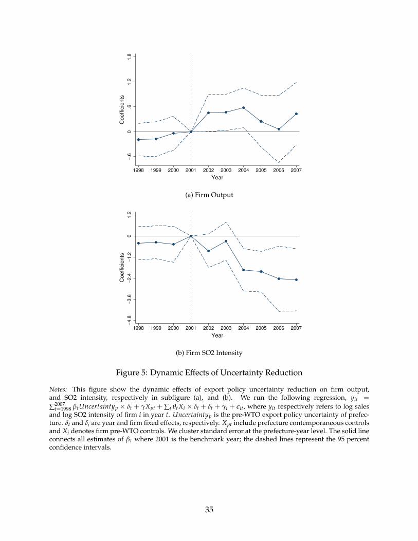
The identification strategy for equation (33) relies on the parallel trends assumptionthat the outcomes in different comparison groups would follow the same time trend inthe absence of treatment. Our estimate of β would be biased if firms located in prefecturesfacing different extents of trade policy uncertainty prior to WTO accession follow differ-ent time paths. To support the parallel trends assumption, we conduct an event studythat takes the following form:

yit =2007

∑t=1998

βtUncertaintyp × δt + γXct + ∑t

θtXi × δt + δt + γi + εit, (36)

All variables in equation (36) follow the same definition as those in equation (33). Ratherthan interacting Uncertaintyp with a Postit dummy, we interact Uncertaintyp with each ofthe year dummy variables, with 2001 being the benchmark year. The event study speci-fication allows us to examine changes in the correlation between a prefecture’s pre-WTOuncertainty and the outcome of interest over time, with each βt measuring the differencein this correlation in year t relative to the year 2001. If the parallel trends assumptionholds, then we expect the estimated βts to be approximately zero throughout the WTOperiod but experience a sharp change after WTO accession.

We test this assumption separately for firm output and emission intensity followingequation (36). We present the estimated coefficients and the 95 percent confidence inter-vals for firm output and emission intensity in Figures (5a) and (5b), respectively. In allfigures, the benchmark year is 2001. We find that before 2001, the estimated coefficientsare indistinguishable from zero. Moreover, the effect on output and SO2 intensity startsin 2001.

5.1.2 Robustness

In this subsection, we employ several empirical exercises to examine the sensitivity of thebaseline estimates. Because our main variation is at the prefecture level, one concern is

16The standard deviation of uncertainty is 0.06545. We multiply the estimated coefficients by this num-ber.

19

that our results are confounded by other concurrent events that occurred at the prefecturelevel. To address this concern, we further control for a set of prefecture variables. First,at the time of the WTO entry, China also changed its import tariffs, eliminated export li-censing requirements, and faced different export quotas, and firms with different contractintensities also responded differently to WTO entry. We control for the value of these vari-ables in 2000 at the prefecture level and interact them with the post dummy to addressthe concern that prefectures were affected differently by WTO accession along these di-mensions. Second, we also control for contemporaneous prefecture GDP and populationdensity. We present the results in Table 3 for firm output, SO2 emissions, and emissionintensity. The results are highly consistent. In columns (1), (3), and (5), we control forthe initial prefecture value of other policy changes interacted with the post dummy; incolumns (2), (4), and (6), we further control for contemporaneous prefecture GDP percapita and population density. The effects on firm output, SO2 emissions and emissionintensity remain largely consistent with those in Table 2, and the estimated coefficientsare not influenced by additional contemporaneous prefecture controls, which suggeststhat our results are highly unlikely to be driven by other concurrent prefecture events.

Relatedly, firms with different ownership status or located in different provinces mayexperience different changes in production or SO2 emissions. One specific concern is thatthese differences are confounded by our uncertainty measure. We therefore address thisconcern by controlling for ownership-year fixed effects and province-year fixed effectsand present the results in Table 4. Our results remain robust.

Another concern is that our main results are driven by the specific construct of the pre-fecture uncertainty measure. To show that our results are robust to the construction of theuncertainty measure, we use four alternative methods to construct the uncertainty mea-sure. First, we use labor instead of exports as our weights and then compute the labor-weighted average value of the NTR gap at the prefecture level. To reflect the fact that Chi-nese exports to the U.S. experience a reduction in tariff uncertainty, we use product-levelChinese exports to the U.S. as our weights in the main exercise. This exercise, however,has two concerns. First, the Chinese exports to the U.S. are endogenous to U.S. policy,and our constructs using endogenous weights may cause biases. Second, this measureomits those exports from China to the U.S. via a third country or region such as HongKong. To demonstrate the robustness of our results, we use all product-level Chinese ex-ports in our second and third measures. Our second measure uses the simple averageNTR gap of all exports from a prefecture; the third measure uses the export-weightedaverage value of the NTR gap of a prefecture. We also calculate the firm-level trade pol-icy uncertainty shock as fourth measures. As in the main exercise, we use the Chinese

20

exports to the U.S. as our weights when we measure uncertainty at the firm level. Table5 presents the results using different proxies for uncertainty. The first three columns ofpanel A use the first alternative uncertainty measure; the last three columns of panel Ause the second alternative uncertainty measure; the first three columns of panel B usethe third alternative uncertainty measure. In the last three columns of panel B, we de-fine uncertainty at firm levels, which measures the uncertainty shock exerted on firms inmore precise ways.17 Notice that we have lost a significant number of observations usingfirm-level uncertainty measures. The results are highly consistent. The reduction in tradepolicy uncertainty significantly increased firm production, reduced firm overall emissionof SO2, and reduced firm SO2 emission per unit of output.

5.1.3 Falsification Test

To rule out the possibility that our main results are spurious and driven by chance, weperform a falsification test. We follow equation (33) to conduct regression analyses basedon randomly assigned false prefecture-level uncertainty to firms, in proportion to theactual uncertainty distribution. We then conduct 500 rounds of randomization and plotthe distribution of estimated coefficients in Figure 6, separately for firm output in sub-figure (a) and firm SO2 emission intensity in sub-figure (b). For firm output, the meanvalue of the estimated coefficient is 0.0069, the standard deviation is 0.2355, and the actualestimate for firm output is depicted by the red vertical line valued at 0.639. For firm SO2emission intensity, the mean value of the estimated coefficient is 0.0626, the standarddeviation is 0.5817, and the actual estimate for firm output is depicted by the red verticalline valued at -1.313. Therefore, it is unlikely that the increases in firm output and declinesin firm SO2 emission intensity reported in Table 2 are driven by chance.

5.2 Heterogeneous effects

To test Predictions 2 and 3, we examine the heterogeneous effects of reduced uncertaintyon firm output and SO2 emissions varied by the strength of SO2 emission control. As wemention in Section 2, firms that are located in TCZs face more stringent SO2 emissionscontrol than firms in non-TCZs. Thus, we expect that the reduction in export policy un-certainty should increase firm output in both TCZs and non-TCZs, but it would reducefirm emission intensity only for firms in TCZs.

17A prefecture may have firms that do not export to the U.S. Thus, defining uncertainty at prefecturelevels is a less precise way to measure the policy uncertainty shock exerted on each firm.

21

We first separately study the average effects for firms in TCZs and non-TCZs followingthe main specification in equation (33). To further test the statistical significance of theeffect difference, we conduct a triple-difference specification following equation (34).

Table 6 presents the results. Columns (1) to (3) study the effects on firm output. Col-umn (1) focuses on firms in TCZs, and column (2) focuses on firms in non-TCZs. Wefind that the reduction in export policy uncertainty leads to increases of firm output inboth TCZs (as shown in column (1)) and non-TCZs (as shown in column (2)). The triple-difference results presented in column (3) suggest insignificant differences in firm outputincreases in TCZs and non-TCZs.

Columns (4) to (6) rerun the exercises in columns (1) to (3) but replace the dependentvariable with log value of firm SO2 emissions. We find that firm-level SO2 emissions inTCZs are significantly reduced when export policy uncertainty decreases (as shown incolumn (4)), whereas the firm-level SO2 emissions are unaffected in non-TCZs (as shownin column (5)). The triple-difference results presented in column (6) suggest that the ef-fect difference in SO2 emissions between firms in TCZs and non-TCZs is significant at 5percent.

Columns (7) to (9) further repeat the exercises with log values of firm SO2 emissionintensity as the dependent variable. Consistent with the effects on firm SO2 emissions,we find that the reduction in export policy uncertainty significantly lowers SO2 emissionintensity in TCZs but does not affect firms in non-TCZs. The difference of the effects onSO2 emission intensity is statistically significant at the 1 percent level.

We have also conducted the effects of reduced uncertainty on other pollution out-comes as our placebo check. Since the emission gap specifically targets SO2, the effectsshould not exist for other types of firm pollution. We use wastewater, fumes, and nitro-gen oxides (NOx) for our placebo check, as our dataset also covers these variables. Table7 presents the results. All regressions control for firm and year fixed effects. In contrastto the results on SO2 in Tables 2, we do not find significant effects on the emission inten-sity of these types of pollution. Moreover, the trade policy uncertainty reduction exertsno heterogeneous effects on these alternative pollutants across regions with different SO2emission control.

These results support our model predictions. When export policy uncertainty de-creases, the overall emission control imposed on firms reduced per firm SO2 emissionsand per firm SO2 emission intensity, but it does not affect firm output. One plausibleexplanation for why firm production (measured by firm output) is not influenced by theemission cap is that firms could improve production efficiency more in the regions withemission caps. We test the mechanisms in greater detail in the sections below.

22

5.3 Mechanism

Emission intensity declined following the reduction in export policy uncertainty, as shownin our previous analyses. It thus becomes natural to ask, what inherent mechanisms areaccounting for this change? In particular, what accounts for the greater emission reduc-tion for firms in TCZs? According to Liu et al. (2018), SO2 generated per unit of fossilfuel during the production process depends on conversion efficiency, desulfurization ef-ficiency, and average sulfur content.18 Therefore, we will analyze the underlying mecha-nisms from the perspective of the relative usage of fossil fuel (coal and fuel) and its sulfurcontent, pollution-control facilities and firm productivity in this section.

5.3.1 Effects on inputs

First, we study firms’ use of energy in Table 8, separately for firms in TCZs and non-TCZs. Column (1) studies the average effect on coal use for all firms, whereas columns(2) and (3) split the sample and study the effect for firms in TCZs and non-TCZs. We findthat, although the reduction in export policy uncertainty on average has a negative butstatistically insignificant effect on coal use, the effects are drastically different for firms inTCZs and firms in non-TCZs. The reduction in uncertainty leads to a decline in coal usefor firms in TCZs but an increase in coal use for firms in non-TCZs. The differences inthe effects are statistically significant, as shown by the coefficient of the triple-interactionterm in column (4).

We then repeat the exercises for fuel use. Column (5) studies the average effect onfuel use for all firms, whereas columns (6) and (7) split the sample and study the effectfor firms in TCZs and non-TCZs. Consistent with the exercise on coal, we find that thereduction in uncertainty has an insignificant effect on fuel use on average, and the effectsare different for firms in TCZs and firms in non-TCZs. The reduction in uncertainty leadsto an insignificant decline in fuel use for firms in TCZs but a significant increase for firmsin non-TCZs. The effect difference is statistically significant (column (8)).

Firms may also substitute away from fossil fuel to other inputs, such as non-pollutingmaterials and labor. We then study the effect on other firm inputs in Table 9. Our datasetreports the total amount of intermediate inputs, which include energy input and material.For firms in TCZs, the reduced uncertainty causes a lower usage of energy but a possibly

18The emissions of SO2 can be expressed as ESO2 = ∑i,j 2× Cj × Ai,j × Si,j × (1− ηi) based on the massbalance method in Liu et al. (2018)), where ESO2 represents the total emissions of SO2; i and j representpower plant i and fuel type j, respectively; Cj is the conversion efficiency to sulfur dioxide from fuel typej; and Ai,j is the annual consumption of fuel type j by power plant i. ηi is the desulfurization efficiencythat varies across different de-SO2 processes; Si.j represents the sulfur content in fuel j of plant i; and 2represents the molecular weight of SO2 that is twice the atomic weight of Si,j.

23

higher use of material, while the effect on total intermediate inputs is ambiguous; firmsin non-TCZs, the reduction in uncertainty promotes firm production and does not reduceenergy use, and therefore, we expect the use of total intermediate inputs to increase. Wepresent the results in columns (1) to (4). Columns (1) to (3) focus on all firms, firms locatedin TCZs and firms located in non-TCZs, respectively. The average effect on intermediateinput use is statistically insignificant, as reported in column (1). Consistent with our ex-pectation, we find that firms in non-TCZs increased their intermediate input use, whereasfirms in TCZs did not significantly change intermediate input use.

The dataset also reports firm total labor employment. If labor is a substitute for fossilfuel, then reduced export policy uncertainty should cause firms in TCZs to increase theirlabor employment. For firms in non-TCZs, however, the expected effect is ambiguous.On the one hand, increases in production scale lead to a higher demand for labor; on theother hand, the higher labor demand in TCZs may drive up labor wages, which reducesdemand for labor.19 We report the results on labor in columns (5) to (8). We find thatthe reduction in uncertainty leads to higher overall labor employment for firms in oursample. The increases in labor are driven solely by firms in TCZs. There is no significanteffect on firms in non-TCZs.

5.3.2 Effects on sulfur content and pollution abatement equipment

Firms may also change the types of coal and fuel to reduce emissions intensity. A moredirect test would be to test the sulfur content used by firms. Moreover, the reduction inemission intensity can be also caused by more abatement equipment. We then examinethe effects of reduced uncertainty on energy sulfur content and abatement equipment,which are two variables available in our dataset.

Table 10 presents the results. Columns (1) to (4) focus on the sulfur content of energyuse, and columns (5) to (8) focus on pollution abatement equipment. We find that thefirms in TCZs significantly reduced the sulfur content when they increased firm outputas a response to the reduction in export policy uncertainty, and they also adopted morepollution-control facilities to remove sulfur emissions. These effects only exist for firms inTCZs and not for firms in non-TCZs. The significant heterogeneous effects are highlightedin the estimated coefficients of the triple-difference exercise in columns (4) and (8).

19Higher demand for labor in TCZs induces labor to be reallocated from non-TCZs to TCZs.

24

5.3.3 Effects on firm productivity

According to the Porter hypothesis, strict environmental regulations can induce firms toupgrade their productivity. We examine this by testing whether firms in TCZs improveproductivity more when export policy uncertainty decreases. In Table 11, we use two dif-ferent measures of TFP. Columns (1) to (4) use the Olley-Pakes method to compute firmTFP, while columns (4) to (8) use the ACF method to compute firm TFP. We follow theprevious exercises and separately examine the average policy effects on firm TFP, the ef-fects on firm TFP in TCZs and effects on firm TFP in non-TCZs. In columns (1) and (5), weshow the average effects. We find that the reduction in export policy uncertainty leads toa higher level of firm TFP.20 We also find that the productivity-improving effects of loweruncertainty are greater for firms in TCZs, which is consistent with our results in Table6 that after export policy uncertainty decreases, firms in TCZs and non-TCZs increasefirm output by comparable magnitudes, but only firms in TCZs reduce SO2 emissionsintensity.

6 Conclusion

This study examines the effects of reducing the uncertainty of trade policy on firms’ pol-lution behavior. We first develop a model to show that the impacts of reducing trade pol-icy uncertainty on firms’ pollution behavior depend on whether an emission cap exists.When a cap exists, reduced uncertainty leads to higher output but lower emission inten-sity. When no cap exists, however, reduced uncertainty increases firm output but has noeffect on emission intensity. We exploit spatial variations in the reductions in trade policyuncertainty caused by U.S. conferral of PNTR status to Chinese exporters and variationsin emission control caused by the TCZs to test the hypotheses. Our empirical evidence isconsistent with the model predictions. We find that the reduction in uncertainty increasesfirm output by comparable magnitudes across regions with different extents of emissioncontrol, but it reduces firm SO2 emission intensity and total firm SO2 emissions only in re-gions with stringent emission control. The decline in SO2 emissions is caused by reduceduse of fossil fuel, less sulfur content in energy use, and more abatement equipment, andfirms substitute away from energy use with more labor. We also find that the reductionin uncertainty and emission control jointly improve firms’ productivity, consistent withthe Porter hypothesis. One implication is that it is not imperative for developing coun-tries to adopt lax environmental regulations to capture gains from globalization. Instead,

20This is consistent with the literature on trade-induced technological upgrading; see, e.g., Bustos (2011).

25

strengthening environmental regulations may promote production efficiency for firms indeveloping countries in times of globalization.

26

References

Acemoglu, D., U. Akcigit, D. Hanley, and W. Kerr (2016). Transition to clean technology.Journal of Political Economy 124, 52–104.

Ackerberg, D., K. Caves, and G. Frazer (2015). Identification properties of recent produc-tion function estimators. Econometrica 83, 2411–2451.

Aghion, P., R. Benabou, R. Martin, and A. Roulet (2020). Environmental preferences andtechnological choices: Is market competition clean or dirty? CEPR Discussion Paper No.DP14581.

Aghion, P., A. Dechezlepretre, D. Hemous, R. Martin, and J. Van Reenen (2016). Carbontaxes, path dependency, and directed technical change: Evidence from the auto indus-try. Journal of Political Economy 124(1), 1–51.

Aichele, R. and G. Felbermayr (2015). Kyoto and carbon leakage: An empirical analysisof the carbon content of bilateral trade. Review of Economics and Statistics 97, 104–115.

Alpert, P., O. Shvainshtein, and P. Kishcha (2012). Aod trends over megacities based onspace monitoring using modis and misr. American Journal of Climate Change 1(3), 117–31.

Amiti, M. and J. Konings (2007). Trade liberalization, intermediate inputs, and produc-tivity: Evidence from indonesia. American Economic Review 97, 1611–1638.

Bai, X., K. Krishna, and H. Ma (2017). How you export matters: Export mode, learningand productivity in china. Journal of International Economics 104, 122–137.

Banerjee, A., E. Duflo, and R. Glennerster (2008). Putting a band-aid on a corpse: Incen-tives for nurses in the indian public health care system. Journal of the European EconomicsAssociation 6(2-3), 487–500.

Barrows, G. and H. Ollivier (2016). Emission intensity and firm dynamics: reallocation,product mix, and technology in india. GRI Working Papers 245.

Brambilla, I., A. Khandelwal, and P. Schott (2010). China’s experience under the multifiberarrangement (mfa) and the agreement on textiles and clothing (atc). NBER WorkingPapers 13346.

Brandt, L., J. Biesebroeck, and Y. Zhang (2009). Creative accounting or creative destruc-tion? firm-level productivity growth in chinese manufacturing. Journal of DevelopmentEconomics 97(2), 339–351.

27

Broda, C. and D. E. Weinstein (2006). Globalization and the Gains From Variety. TheQuarterly Journal of Economics 121(2), 541–585.

Broner, F., P. Bustos, and V. M. Carvalho (2012). Sources of comparative advantage inpolluting industries. NBER Working Papers 18337.

Bustos, P. (2011). Trade liberalization, exports, and technology upgrading: Evidence onthe impact of mercosur on argentinian firms. American Economic Review 101(1), 304–340.

Cherniwchan, J. (2017). Trade liberalization and the environment: Evidence from naftaand u.s. manufacturing. Journal of International Economics 105, 130–149.

Crowley, M., N. Meng, and H. Song (2018). Tariff scares: Trade policy uncertainty andforeign market entry by chinese firms. Journal of International Economics 114, 96–115.

Cui, J., H. Lapan, and G. Moschini (2016). Productivity, export, and environmental per-formance: Air pollutants in the united states. American Journal of Agricultural Eco-nomics 98(2), 447–467.

Dekle, R., J. Eaton, and S. Kortum (2007). Unbalanced Trade. The American EconomicReview 97(2), 351–355.

Dekle, R., J. Eaton, and S. Kortum (2008). Global Rebalancing with Gravity: Measuringthe Burden of Adjustment. IMF Staff Papers 55(3), 511–540.

Erten, B. and J. Leight (2019). Exporting out of agriculture: The impact of wto accessionon structural transformation in china. Review of Economics and Statistics.

Facchini, G., M. Y. Liu, A. M. Mayda, and M. Zhou (2019). China’s ”great migration”: Theimpact of the reduction in trade policy uncertainty. Journal of International Economics 120,126–144.

Fan, H., Y. A. Li, and S. R. Yeaple (2015). Trade liberalization, quality, and export prices.Review of Economics and Statistics 97, 1033–1051.

Fan, H., Y. A. Li, and S. R. Yeaple (2018). On the relationship between quality and produc-tivity: Evidence from china’s accession to the wto. Journal of International Economics 110,28–49.

Feenstra, R. C., J. Romalis, and P. K. Schott (2002). U.s. imports, exports, and tariff data,1989-2001. NBER Working Papers 9387.

28

Forslid, R., T. Okubo, and K. H. Ulltveit-Moe (2018). Why are firms that export cleaner?international trade, abatement and environmental emissions. Journal of EnvironmentalEconomics and Management 91, 166–183.

Gan, L., M. A. Hernandez, and M. Shuang (2016). The higher costs of doing businessin china: Minimum wages and firms’ export behavior. Journal of International Eco-nomics 100, 81–94.

Garred, J. (2018). The persistence of trade policy in china after wto accession. Journal ofInternational Economics 114, 130–142.

Greenstone, M. and R. Hanna (2014). Environmental regulations, air and water pollution,and infant mortality in india. American Economic Review 104(10), 3038–3072.

Gutierrez, E. and K. Teshima (2018). Abatement expenditures, technology choice, andenvironmental performance: Evidence from firm responses to import competition inmexico. Journal of Development Economics 133, 264–274.

Handley, K. and N. Limao (2017). Policy uncertainty, trade and welfare: Theory andevidence for china and the u.s. American Economic Review 107(9), 2731–83.

Hanna, R. (2010). Us environmental regulation and fdi: Evidence from a panel of us-basedmultinational firms. American Economic Journal: Economic Policy 2, 158–189.

Holladay, J. S. (2016). Exporters and the environment. Canadian Journal of Economics 49,147–172.

Hsieh, C.-T. and R. Ossa (2016). A global view of productivity growth in China. Journal ofInternational Economics 102, 209–224.

Imbruno, M. (2019). Importing under trade policy uncertainty: Evidence from china.Journal of Comparative Economics 47(4), 806–826.

Levinson, J. and S. Taylor (2008). Unmasking the pollution haven effect. InternationalEconomic Review 49, 223–254.

Liu, H., B. Wu, P. Shao, X. Liu, C. Zhu, Y. Wang, Y. Wu, Y. Xue, J. Gao, Y. Hao, and H. Tian(2018). A regional high-resolution emission inventory of primary air pollutants in 2012for beijing and the surrounding five provinces of north china. Atmospheric Environ-ment 181, 20–33.

29

Melitz, M. J. (2003). The Impact of Trade on Intra-Industry Reallocations and AggregateIndustry Productivity. Econometrica 71(6), 1695–1725.

Nunn, N. (2007). Relationship-specificity, incomplete contracts, and the pattern of trade.The Quarterly Journal of Economics 122(2), 569–600.

Olley, G. S. and A. Pakes (1996). The dynamics of productivity in the telecommunicationsequipment industry. Econometrica 64, 1263–1297.

Pierce, J. R. and P. K. Schott (2016). The surprisingly swift decline of u.s. manufacturingemployment. American Economic Review 106(7), 1632–62.

Porter, M. E. and C. Van der Linde (1995). Toward a new conception of the environment-competitiveness relationship. Journal of Economic Perspectives 9(4), 97–118.

Shapiro, J. S. and R. Walker (2018). Why Is Pollution from US Manufacturing Declining?The Roles of Environmental Regulation, Productivity, and Trade. 108(12), 3814–3854.

30

4°N

10°N

16°N

108°E 113°E 118°E20°N

30°N

40°N

50°N

70°E 80°E 90°E 100°E 110°E 120°E 130°E 140°E

Non−Two−Control Zones Two−Control Zones

Figure 1: Geographic Locations of Two-Control Zones and Non-Two-Control Zones

Notes: This figure presents the geographic locations of prefectures in the two-control zones (colored in red)and prefectures in the non-two-control zones (colored in blue).

31

Non−Two−Control Zones Two−Control Zones

1999 2000 2001 2002 2003 2004 2005 2006 1999 2000 2001 2002 2003 2004 2005 2006

100

150

200

250

Year

Sca

led

valu

e (y

ear

1999

=10

0)

GDP SO2 emission

Figure 2: Total Output and SO2 Emission in Two-Control Zones and Non-Two-ControlZones

Notes: This figure plots the total GDP and total SO2 emission in two-control-zones (TCZs) and non-two-control-zones (non-TCZs). The data for GDP are drawn from CEIC database, and the SO2 emission data arefrom China Statistical Yearbook on Environment, published by the Ministry of Ecology and Environmentof China. We treat 1999 as the benchmark year (value=100). Although GDP has been rising rapidly in bothregions, the SO2 emission in TCZs remains relatively stagnant between 1999 and 2006, which reveals arelatively more stringent SO2 emission control.

32

0 0.2 0.4 0.6 0.8 1

Uncertainty Reduction ( 2)

-0.01

0

0.01

0.02

0.03

0.04

0.05

0.06

0.07

Out

put

Output

0 0.2 0.4 0.6 0.8 1

Uncertainty Reduction ( 2)

-0.03

-0.02

-0.01

0

0.01

0.02

0.03

0.04

0.05

0.06

0.07

Em

issi

on

Emission

0 0.2 0.4 0.6 0.8 1

Uncertainty Reduction ( 2)

-0.08

-0.07

-0.06

-0.05

-0.04

-0.03

-0.02

-0.01

0

Em

issi

on in

tens

ity

Emission Intensity

0 0.2 0.4 0.6 0.8 1

Uncertainty Reduction ( 2)

-0.04

-0.03

-0.02

-0.01

0

0.01

0.02

0.03

0.04

0.05

0.06

(1-3

)^(1

/,)

(1-3)^(1/,)

;=0;=0.25;=0.5;=0.75;=1

Figure 3: The Simulated Effects of Uncertainty Reduction on Production and Emission(Emission Cap κ = 0.975)

Notes: This figure presents the simulated effects of a reduction in export policy uncertainty on firm totaloutput, total emission, emission intensity, and inputs used for production, respectively. We set the emissioncap κ to be 0.975. We plots the effects for different levels of environment regulation stringency, characterizedby parameter ρ. A higher value of ρ corresponds to more stringent emission control.

33

0 0.1 0.2 0.3 0.4 0.5 0.6 0.7 0.8 0.9 1

Uncertainty Reduction ( 2)

0

0.01

0.02

0.03

0.04

0.05

0.06

0.07

0.08

0.09

Em

issi

on c

osts

Emission Costs

;=0;=0.25;=0.5;=0.75;=1

Figure 4: The Simulated Effects of Uncertainty Reduction on Emission Costs (EmissionCap κ = 0.975)

Notes: This figure presents the simulated effects of a reduction in export policy uncertainty on firm emissioncosts. We set the emission cap κ to be 0.975. We plots the relations between uncertainty reduction andemission cost for different levels of environment regulation stringency, which is characterized by ρ. Ahigher value of ρ corresponds to more stringent emission control.

34

−.6

0.6

1.2

1.8

Co

eff

icie

nts

1998 1999 2000 2001 2002 2003 2004 2005 2006 2007

Year

(a) Firm Output

−4

.8−

3.6

−2

.4−

1.2

01

.2

Co

eff

icie

nts

1998 1999 2000 2001 2002 2003 2004 2005 2006 2007

Year

(b) Firm SO2 Intensity

Figure 5: Dynamic Effects of Uncertainty Reduction

Notes: This figure show the dynamic effects of export policy uncertainty reduction on firm output,and SO2 intensity, respectively in subfigure (a), and (b). We run the following regression, yit =

∑2007t=1998 βtUncertaintyp × δt + γXpt + ∑t θtXi × δt + δt + γi + εit, where yit respectively refers to log sales

and log SO2 intensity of firm i in year t. Uncertaintyp is the pre-WTO export policy uncertainty of prefec-ture. δt and δi are year and firm fixed effects, respectively. Xpt include prefecture contemporaneous controlsand Xi denotes firm pre-WTO controls. We cluster standard error at the prefecture-year level. The solid lineconnects all estimates of βt where 2001 is the benchmark year; the dashed lines represent the 95 percentconfidence intervals.

35

0.5

11

.52

−.5 0 .5 1

Estimated Coefficient

Density Actual estimate

(a) Firm Output

0.2

.4.6

.8

−2 −1 0 1 2

Estimated Coefficient

Density Actual estimate

(b) Firm SO2 Intensity

Figure 6: Distribution of estimates in 500 randomization tests

Notes: In this exercise, we follow equation (33) to conduct regression analyses based on randomly assigneduncertainty. We assign false prefecture-level uncertainty to firms randomly in proportion to the actual un-certainty distribution. We then conduct 500 rounds of randomization and plot the distribution of estimatedcoefficients in the figures above, separately for firm output and firm SO2 emission intensity. For firm out-put, the mean value of estimated coefficient is 0.0069 and the standard deviation is 0.2355, and the actualestimate for firm output is depicted by the red vertical line valued at 0.639. For firm SO2 emission inten-sity, the mean value of estimated coefficient is 0.0626 and the standard deviation is 0.5817, and the actualestimate for firm output is depicted by the red vertical line valued at -1.313.

36

Table 1: Summary Statistics

Variable Obs Mean Std.Dev. P10 P50 P90Dependent VariablesLog Output 58979 8.007 1.607 6.205 7.895 10.050Log SO2 Emission 58979 10.050 2.065 7.455 10.150 12.500Log SO2 Emission Intensity 58979 2.038 2.129 -0.676 2.239 4.504Log Wastewater Intensity 51623 2.909 1.962 0.425 3.010 5.317Log Fumes Intentsity 54971 1.697 2.702 -1.609 1.594 5.409Log NOx 17957 -6.561 4.235 -10.370 -7.871 1.216Log Coal 53607 6.715 2.571 3.714 7.080 9.398Log Fuel 13275 3.800 3.237 0.000 4.078 8.075Log Facilities 52398 1.143 0.803 0.000 1.099 2.197Sulfur Content 13154 0.132 0.642 0.000 0.000 0.580Log Employment 58836 5.951 1.111 4.605 5.886 7.378Log Intermediate Inputs 58698 10.220 1.542 8.465 10.100 12.200TFP(OP) 58495 0.781 1.458 -1.373 1.045 2.399TFP(ACF) 58495 3.892 1.812 2.203 3.487 6.303

Independent VariablesUncertainty(Base) 58979 0.054 0.047 0.005 0.049 0.092Uncertainty(All Exp. Weighted) 58979 0.346 0.115 0.182 0.371 0.490Uncertainty(Employment Weighted) 65011 0.244 0.069 0.142 0.256 0.320Uncertainty(Simple Avg.) 58979 0.392 0.084 0.297 0.405 0.472Uncertainty(Firm Level) 8221 0.018 0.065 0.000 0.000 0.030Initial Log Output 58979 7.910 1.480 6.215 7.824 9.810Initial Log SO2 Emission 58979 10.180 2.033 7.659 10.290 12.600SOE (=1 if SOE) 58979 0.389 0.487 0.000 0.000 1.000Log GDP per capita 58522 9.295 0.810 8.335 9.223 10.390Log pop 58522 6.049 0.677 5.233 6.118 6.775TCZ (=1 if TCZ) 58979 0.744 0.437 0.000 1.000 1.000Import Tariff 58439 15.010 8.205 8.464 14.130 20.790Export License 58699 0.166 0.273 0.009 0.042 0.597Contract Intensity 58979 0.509 0.113 0.344 0.528 0.630Export Quota 58979 0.156 0.141 0.006 0.139 0.333

37

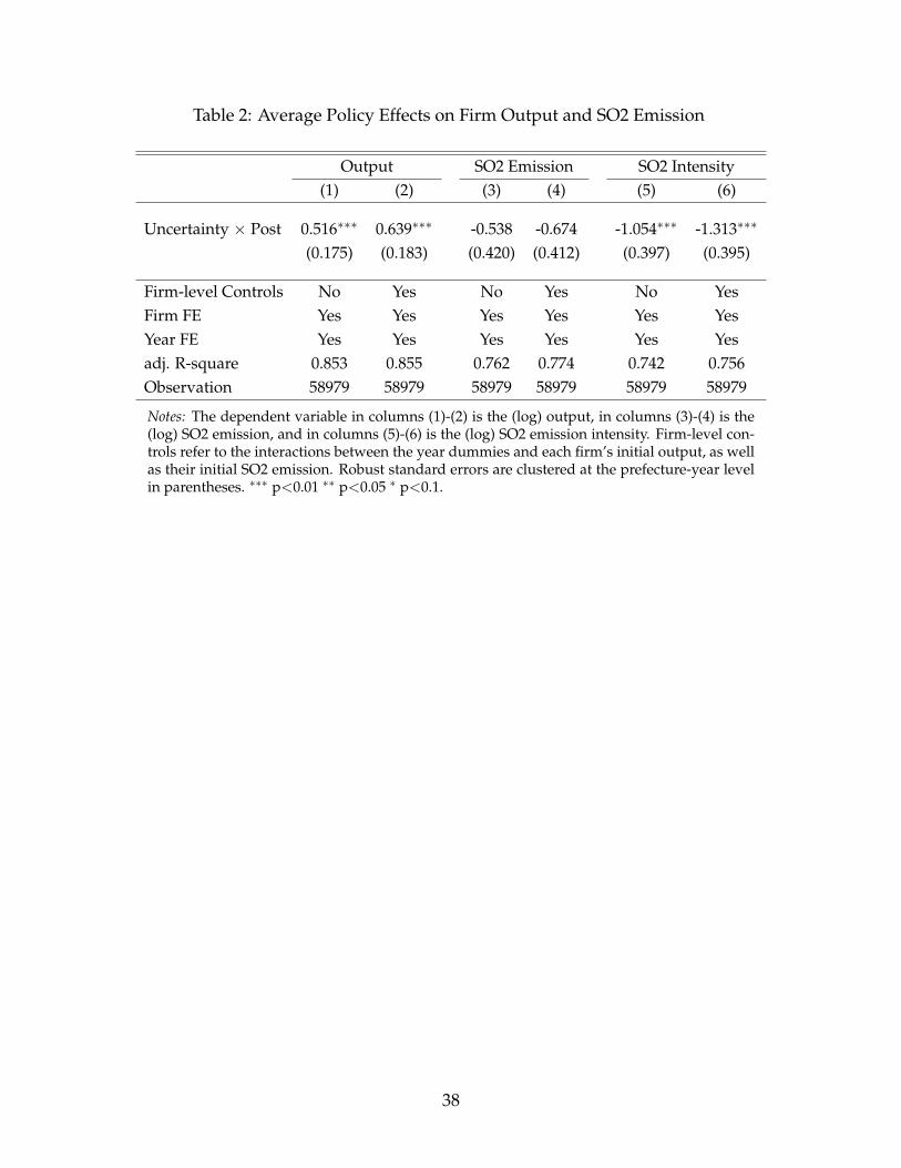
Table 2: Average Policy Effects on Firm Output and SO2 Emission

Output SO2 Emission SO2 Intensity(1) (2) (3) (4) (5) (6)

Uncertainty × Post 0.516∗∗∗ 0.639∗∗∗ -0.538 -0.674 -1.054∗∗∗ -1.313∗∗∗

(0.175) (0.183) (0.420) (0.412) (0.397) (0.395)

Firm-level Controls No Yes No Yes No YesFirm FE Yes Yes Yes Yes Yes YesYear FE Yes Yes Yes Yes Yes Yesadj. R-square 0.853 0.855 0.762 0.774 0.742 0.756Observation 58979 58979 58979 58979 58979 58979

Notes: The dependent variable in columns (1)-(2) is the (log) output, in columns (3)-(4) is the(log) SO2 emission, and in columns (5)-(6) is the (log) SO2 emission intensity. Firm-level con-trols refer to the interactions between the year dummies and each firm’s initial output, as wellas their initial SO2 emission. Robust standard errors are clustered at the prefecture-year levelin parentheses. ∗∗∗ p<0.01 ∗∗ p<0.05 ∗ p<0.1.

38

Table 3: Average Policy Effects Controlling For Contemporaneous Prefectural Controls

Output SO2 Emission SO2 Intensity

(1) (2) (3) (4) (5) (6)

Uncertainty × Post 0.806∗∗∗ 0.767∗∗∗ -0.218 -0.215 -1.024∗∗ -0.982∗∗

(0.186) (0.184) (0.417) (0.421) (0.402) (0.405)Log GDP per capita 0.095∗∗∗ 0.008 -0.088

(0.028) (0.075) (0.085)Log pop 0.058∗∗ 0.036 -0.022

(0.024) (0.048) (0.047)

City-level Shocks Yes Yes Yes Yes Yes YesFirm-level Controls Yes Yes Yes Yes Yes YesFirm FE Yes Yes Yes Yes Yes YesYear FE Yes Yes Yes Yes Yes Yesadj. R-square 0.855 0.855 0.776 0.777 0.756 0.756Observation 58439 58439 58439 58439 58439 58439

Notes: The dependent variable in columns (1)-(2) is the (log) output, in columns (3)-(4) is the(log) SO2 emission, and in columns (5)-(6) is the (log) SO2 emission intensity. Firm-level con-trols refer to the interactions between the year dummies and each firm’s initial output, as wellas their initial SO2 emission. City-level shocks include import tariffs, export licensing, exportquotas, and contract intensities interacted with year dummies. Robust standard errors areclustered at the prefecture-year level in parentheses. ∗∗∗ p<0.01 ∗∗ p<0.05 ∗ p<0.1.

39

Table 4: Robustness Checks: Policy Effects with More Fixed Effects

Output SO2 Emission SO2 Intensity

(1) (2) (3) (4) (5) (6)

Uncertainty × Post 0.629∗∗∗ 0.681∗∗∗ -0.845∗∗ -0.827∗∗ -1.474∗∗∗ -1.509∗∗∗

(0.183) (0.203) (0.413) (0.389) (0.396) (0.383)

Firm-level Controls Yes Yes Yes Yes Yes YesOwnership-Year FE Yes Yes Yes Yes Yes YesProvince-Year FE No Yes No Yes No YesFirm FE Yes Yes Yes Yes Yes YesYear FE Yes Yes Yes Yes Yes Yesadj. R-square 0.855 0.856 0.775 0.780 0.756 0.762Observation 58979 58979 58979 58979 58979 58979

Notes: The dependent variable in columns (1)-(2) is the (log) output, in columns (3)-(4) is the(log) SO2 emission, and in columns (5)-(6) is the (log) SO2 emission intensity. Firm-level controlsrefer to the interactions between the year dummies and each firm’s initial output, as well astheir initial SO2 emission. Robust standard errors are clustered at the prefecture-year level inparentheses. ∗∗∗ p<0.01 ∗∗ p<0.05 ∗ p<0.1.

40

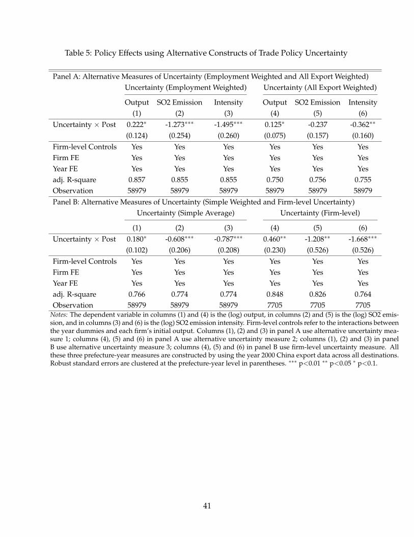
Table 5: Policy Effects using Alternative Constructs of Trade Policy Uncertainty

Panel A: Alternative Measures of Uncertainty (Employment Weighted and All Export Weighted)Uncertainty (Employment Weighted) Uncertainty (All Export Weighted)

Output SO2 Emission Intensity Output SO2 Emission Intensity(1) (2) (3) (4) (5) (6)

Uncertainty × Post 0.222∗ -1.273∗∗∗ -1.495∗∗∗ 0.125∗ -0.237 -0.362∗∗

(0.124) (0.254) (0.260) (0.075) (0.157) (0.160)Firm-level Controls Yes Yes Yes Yes Yes YesFirm FE Yes Yes Yes Yes Yes YesYear FE Yes Yes Yes Yes Yes Yesadj. R-square 0.857 0.855 0.855 0.750 0.756 0.755Observation 58979 58979 58979 58979 58979 58979Panel B: Alternative Measures of Uncertainty (Simple Weighted and Firm-level Uncertainty)

Uncertainty (Simple Average) Uncertainty (Firm-level)

(1) (2) (3) (4) (5) (6)Uncertainty × Post 0.180∗ -0.608∗∗∗ -0.787∗∗∗ 0.460∗∗ -1.208∗∗ -1.668∗∗∗

(0.102) (0.206) (0.208) (0.230) (0.526) (0.526)Firm-level Controls Yes Yes Yes Yes Yes YesFirm FE Yes Yes Yes Yes Yes YesYear FE Yes Yes Yes Yes Yes Yesadj. R-square 0.766 0.774 0.774 0.848 0.826 0.764Observation 58979 58979 58979 7705 7705 7705

Notes: The dependent variable in columns (1) and (4) is the (log) output, in columns (2) and (5) is the (log) SO2 emis-sion, and in columns (3) and (6) is the (log) SO2 emission intensity. Firm-level controls refer to the interactions betweenthe year dummies and each firm’s initial output. Columns (1), (2) and (3) in panel A use alternative uncertainty mea-sure 1; columns (4), (5) and (6) in panel A use alternative uncertainty measure 2; columns (1), (2) and (3) in panelB use alternative uncertainty measure 3; columns (4), (5) and (6) in panel B use firm-level uncertainty measure. Allthese three prefecture-year measures are constructed by using the year 2000 China export data across all destinations.Robust standard errors are clustered at the prefecture-year level in parentheses. ∗∗∗ p<0.01 ∗∗ p<0.05 ∗ p<0.1.

41

Tabl

e6:

Het

erog

enei

tyPo

licy

Effe

cts

byTw

o-C

ontr

ol-Z

ones

(TC

Z)

Out

put

SO2

Emis

sion

SO2

Inte

nsit

y

(1)

(2)

(3)

(4)

(5)

(6)

(7)

(8)

(9)

Unc

erta

inty×

Post

0.76

7∗∗∗

0.50

8∗∗

0.49

5∗∗

-2.2

93∗∗∗

0.33

00.

301

-1.5

26∗∗

-0.1

78-0

.194

(0.2

84)

(0.2

32)

(0.2

31)

(0.6

18)

(0.4

02)

(0.4

19)

(0.6

59)

(0.4

14)

(0.4

25)

Unc

erta

inty×

Post×

TCZ

0.26

6-1

.896∗∗

-2.1

62∗∗∗

(0.3

68)

(0.7

81)

(0.7

57)

Post×

TCZ

0.00

30.

046

0.04

3(0

.026

)(0

.056

)(0

.056

)

Firm

-lev

elC

ontr

ols

Yes

Yes

Yes

Yes

Yes

Yes

Yes

Yes

Yes

Firm

FEYe

sYe

sYe

sYe

sYe

sYe

sYe

sYe

sYe

sYe

arFE

Yes

Yes

Yes

Yes

Yes

Yes

Yes

Yes

Yes

adkj

.R-s

quar

e0.

860

0.83

60.

855

0.76

50.

756

0.77

40.

780

0.72

20.

756

Obs

erva

tion

4387

115

108

5897

943

871

1510

858

979

4387

115

108

5897

9

Not

es:

Col

umns

(1),

(4)

and

(7)

use

subs

ampl

eof

TCZ

;col

umns

(2),

(5)

and

(8)

use

subs

ampl

eof

non-

TCZ

;col

umns

(3),

(6)

and

(9)

use

who

lesa

mpl

e,T

hede

pend

ent

vari

able

inco

lum

ns(1

)-(3

)is

the

(log

)ou

tput

,in

colu

mns

(4)-

(6)

isth

e(l

og)

SO2

emis

sion

,and

inco

lum

ns(7

)-(9

)is

the

(log

)SO

2em

issi

onin

tens

ity.

Firm

-lev

elco

ntro

lsre

fer

toth

ein

tera

ctio

nsbe

twee

nth

eye

ardu

mm

ies

and

each

firm

’sin

itia

lou

tput

,as

wel

las

thei

rin

itia

lSO

2em

issi

on.

Rob

ust

stan

dard

erro

rsar

ecl

uste

red

atth

epr

efec

ture

-yea

rle

vel

inpa

rent

hese

s.∗∗∗

p<

0.01∗∗

p<

0.05∗

p<

0.1.

42

Tabl

e7:

Polic

yEf

fect

son

Oth

erFi

rmPo

lluta

nts

Was

tew

ater

Inte

nsit

yFu

mes

Inte

nsit

yN

Ox

Inte

nsit

y

(1)

(2)

(3)

(4)

(5)

(6)

(7)

(8)

(9)

(10)

(11)

(12)

All

TC

Zno

n-TC

ZA

llA

llTC

Zno

n-TC

ZA

llA

llTC

Zno

n-TC

ZA

ll

Unc

erta

inty×

Post

-0.0

470.

241

-0.2

78-0

.242

-0.4

04-0

.893

0.19

70.

172

-1.0

17-0

.287

-1.2

93-1

.426

(0.3

16)

(0.4

75)

(0.4

13)

(0.4

26)

(0.4

22)

(0.6

06)

(0.5

33)

(0.5

33)

(0.7

09)

(1.0

39)

(0.9

10)

(0.9

38)

Unc

erta

inty×

Post×

TCZ

0.36

5-1

.065

1.05

1

(0.6

38)

(0.8

08)

(1.3

98)

Post×

TC

Z-0

.007

-0.0

22-0

.249∗∗∗

(0.0

46)

(0.0

71)

(0.0

94)

Firm

-lev

elC

ontr

ols

Yes

Yes

Yes

Yes

Yes

Yes

Yes

Yes

Yes

Yes

Yes

Yes

Firm

FEYe

sYe

sYe

sYe

sYe

sYe

sYe

sYe

sYe

sYe

sYe

sYe

s

Year

FEYe

sYe

sYe

sYe

sYe

sYe

sYe

sYe

sYe

sYe

sYe

sYe

s

adj.

R-s

quar

e0.

756

0.75

50.

757

0.75

60.

811

0.82

00.

773

0.81

10.

883

0.88

00.

893

0.88

3

Obs

erva

tion

4760

235

329

1227

347

602

5097

237

578

1339

450

972

1784

014

115

3725

1784

0

Not

es:

The

spec

ifica

tion

s(2

),(6

)an

d(1

0)us

esu

bsam

ple

ofTC

Z;s

peci

ficat

ions

(3),

(7)

and

(11)

use

subs

ampl

eof

non-

TCZ

;spe

cific

atio

ns(1

),(4

),(5

),(8

),(9

)an

d(1

2)us

ew

hole

sam

ple,

The

depe

nden

tva

riab

lein

spec

ifica

tion

s(1

)-(4

)is

the

(log

)w

aste

wat

erem

issi

onin

tens

ity,

insp

ecifi

cati

ons

(5)-

(8)

isth

e(l

og)

fum

eem

issi

onin

tens

ity,

and

insp

ecifi

cati

ons

(9)-

(12)

isth

e(l

og)

nitr

ogen

oxid

esem

issi

onin

tens

ity.

Firm

-lev

elco

ntro

lsre

fer

toth

ein

tera

ctio

nsbe

twee

nth

eye

ardu

mm

ies

and

each

firm

’sin

itia

lout

put,

asw

ella

sth

eir

init

ialS

O2

emis

sion

.Rob

usts

tand

ard

erro

rsco

rrec

ted

for

clus

teri

ngat

the

city

-yea

rle

veli

npa

rent

hese

s.∗∗∗

p<

0.01∗∗

p<

0.05∗

p<

0.1.

43

Tabl

e8:

Polic

yEf

fect

son

Ener

gyU

se

Coa

lFu

el(1

)(2

)(3

)(4

)(5

)(6

)(7

)(8

)A

llT

CZ

non-

TC

ZA

llA

llT

CZ

non-

TC

ZA

ll

Unc

erta

inty×

Post

-0.2

93-1

.483∗

1.28

8∗∗∗

1.19

8∗∗

0.97

3-1

.333

5.66

8∗∗∗

5.40

1∗∗∗

(0.5

15)

(0.7

87)

(0.4

75)

(0.5

29)

(1.3

13)

(1.5

69)

(1.9

98)

(2.0

00)

Unc

erta

inty×

Post×

TCZ

-2.8

42∗∗∗

-6.9

32∗∗∗

(0.9

64)

(2.5

52)

Post×

TCZ

-0.0

970.

786∗∗∗

(0.0

62)

(0.1

96)

Firm

-lev

elC

ontr

ols

Yes

Yes

Yes

Yes

Yes

Yes

Yes

Yes

Firm

FEYe

sYe

sYe

sYe

sYe

sYe

sYe

sYe

sYe

arFE

Yes

Yes

Yes

Yes

Yes

Yes

Yes

Yes

adkj

.R-s

quar

e0.

932

0.92

70.

947

0.93

20.

652

0.66

10.

584

0.65

3O

bser

vati

on53

607

3916

514

442

5360

713

275

1134

219

3313

275

Not

es:

Col

umns

(1),

(4),

(5)

and

(8)

use

who

lesa

mpl

e;co

lum

ns(2

)an

d(6

)us

esu

bsam

ple

offir

ms

inTC

Zs;

colu

mns

(3)

and

(7)

use

subs

ampl

eof

firm

sin

non-

TC

Zs.

The

depe

nden

tvar

iabl

ein

colu

mns

(1)-

(4)i

sth

e(l

og)c

onsu

mpt

ion

ofco

al,i

nco

lum

ns(5

)-(8

)is

the

(log

)co

nsum

ptio

nof

fule

.Fi

rm-l

evel

cont

rols

refe

rto

the

inte

ract

ions

betw

een

the

year

dum

mie

san

dea

chfir

m’s

init

ialo

utpu

t,as

wel

las

thei

rin

itia

lSO

2em

issi

on.R

obus

tsta

ndar

der

rors

are

clus

tere

dat

the

pref

ectu

re-y

ear

leve

lin

pare

nthe

ses∗∗∗

p<

0.01∗∗

p<

0.05

∗p<

0.1.

44

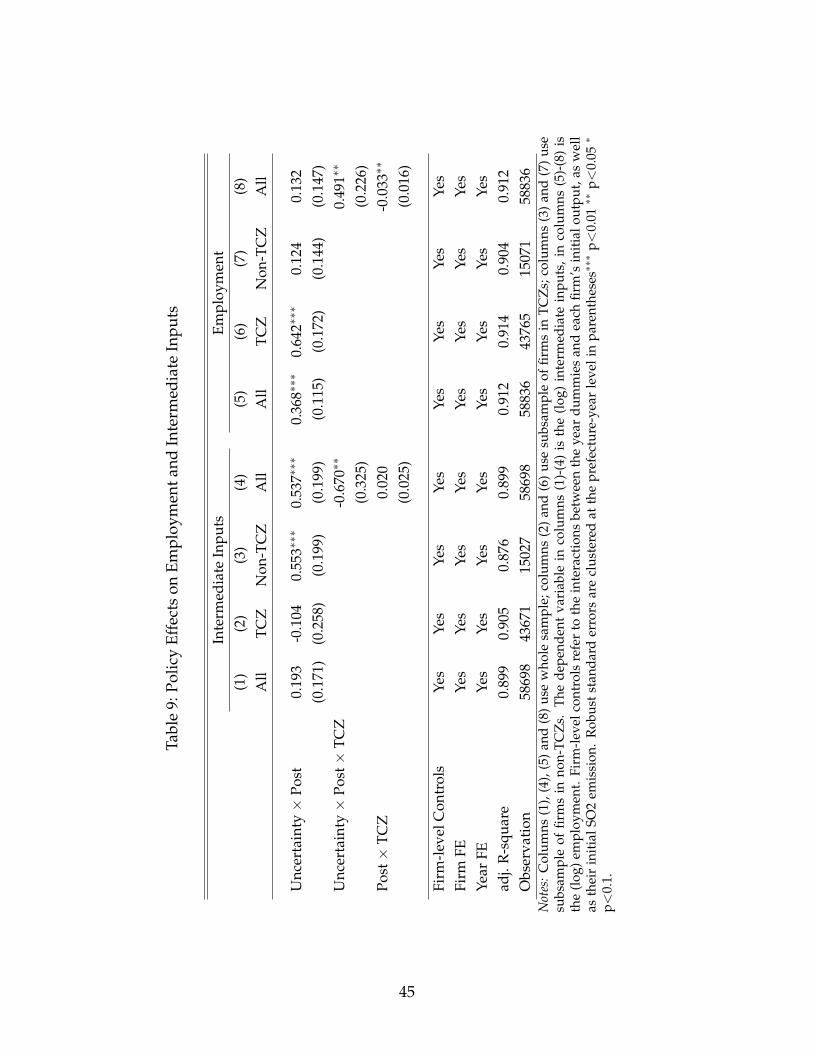
Tabl

e9:

Polic

yEf

fect

son

Empl

oym

enta

ndIn

term

edia

teIn

puts

Inte

rmed

iate

Inpu

tsEm

ploy

men

t(1

)(2

)(3

)(4

)(5

)(6

)(7

)(8

)A

llT

CZ

Non

-TC

ZA

llA

llT

CZ

Non

-TC

ZA

ll

Unc

erta

inty×

Post

0.19

3-0

.104

0.55

3∗∗∗

0.53

7∗∗∗

0.36

8∗∗∗

0.64

2∗∗∗

0.12

40.

132

(0.1

71)

(0.2

58)

(0.1

99)

(0.1

99)

(0.1

15)

(0.1

72)

(0.1

44)

(0.1

47)

Unc

erta

inty×

Post×

TCZ

-0.6

70∗∗

0.49

1∗∗

(0.3

25)

(0.2

26)

Post×

TCZ

0.02

0-0

.033∗∗

(0.0

25)

(0.0

16)

Firm

-lev

elC

ontr

ols

Yes

Yes

Yes

Yes

Yes

Yes

Yes

Yes

Firm

FEYe

sYe

sYe

sYe

sYe

sYe

sYe

sYe

sYe

arFE

Yes

Yes

Yes

Yes

Yes

Yes

Yes

Yes

adj.

R-s

quar

e0.

899

0.90

50.

876

0.89

90.

912

0.91

40.

904

0.91

2O

bser

vati

on58

698

4367

115

027

5869

858

836

4376

515

071

5883

6N

otes

:C

olum

ns(1

),(4

),(5

)an

d(8

)us

ew

hole

sam

ple;

colu

mns

(2)

and

(6)

use

subs

ampl

eof

firm

sin

TCZ

s;co

lum

ns(3

)an

d(7

)us

esu

bsam

ple

offir

ms

inno

n-T

CZ

s.T

hede

pend

ent

vari

able

inco

lum

ns(1

)-(4

)is

the

(log

)in

term

edia

tein

puts

,in

colu

mns

(5)-

(8)

isth

e(l

og)

empl

oym

ent.

Firm

-lev

elco

ntro

lsre

fer

toth

ein

tera

ctio

nsbe

twee

nth

eye

ardu

mm

ies

and

each

firm

’sin

itia

lout

put,

asw

ell

asth

eir

init

ialS

O2

emis

sion

.R

obus

tst

anda

rder

rors

are

clus

tere

dat

the

pref

ectu

re-y

ear

leve

lin

pare

nthe

ses∗∗∗

p<

0.01∗∗

p<

0.05∗

p<

0.1.

45

Tabl

e10

:Pol

icy

Effe

cts

onSu

lfur

Con

tent

and

Pollu

tion

-con

trol

Faci

lity

Sulf

urco

nten

tFa

cilit

y(1

)(2

)(3

)(4

)(5

)(6

)(7

)(8

)A

llT

CZ

non-

TC

ZA

llA

llT

CZ

non-

TC

ZA

ll

Unc

erta

inty×

Post

-0.3

57∗∗

-0.6

43∗∗

-0.1

12-0

.132

0.34

3∗∗∗

0.67

1∗∗∗

0.04

60.

042

(0.1

43)

(0.2

81)

(0.0

89)

(0.1

12)

(0.1

29)

(0.2

10)

(0.1

47)

(0.1

46)

Unc

erta

inty×

Post×

TCZ

-0.5

12∗

0.60

7∗∗

(0.2

95)

(0.2

57)

Post×

TCZ

0.06

1∗∗

-0.0

26(0

.025

)(0

.021

)

Firm

-lev

elC

ontr

ols

Yes

Yes

Yes

Yes

Yes

Yes

Yes

Yes

Firm

FEYe

sYe

sYe

sYe

sYe

sYe

sYe

sYe

sYe

arFE

Yes

Yes

Yes

Yes

Yes

Yes

Yes

Yes

adkj

.R-s

quar

e0.

510

0.49

40.

744

0.51

00.

736

0.74

50.

703

0.73

6O

bser

vati

on13

154

9918

3236

1315

452

398

3881

913

579

5239

8N

otes

:C

olum

ns(1

),(4

),(5

)an

d(8

)us

ew

hole

sam

ple;

colu

mns

(2)

and

(6)

use

subs

ampl

eof

firm

sin

TCZ

s;co

lum

nsin

(3)

and

(7)

use

subs

ampl

eof

firm

sin

non-

TC

Zs.

The

depe

nden

tvar

iabl

ein

colu

mns

(1)-

(4)i

sth

esu

lfur

cont

ento

fcoa

l,in

colu

mns

(5)-

(8)i

sth

e(l

og)

num

ber

ofof

f-ga

str

eatm

ent

faci

litie

s.Fi

rm-l

evel

cont

rols

refe

rto

the

inte

ract

ions

betw

een

the

year

dum

mie

san

dea

chfir

m’s

init

ialo

utpu

t,as

wel

las

thei

rin

itia

lSO

2em

issi

on.

Rob

ust

stan

dard

erro

rsar

ecl

uste

red

atth

epr

efec

ture

-yea

rle

veli

npa

rent

hese

s.∗∗∗

p<

0.01∗∗

p<

0.05∗

p<

0.1.

46

Tabl

e11

:Pol

icy

Effe

cts

onFi

rmTo

talF

acto

rPr

oduc

tivi

ty

TFP

(OP)

TFP

(AC

F)(1

)(2

)(3

)(4

)(5

)(6

)(7

)(8

)A

llT

CZ

Non

-TC

ZA

llA

llT

CZ

Non

-TC

ZA

ll

Unc

erta

inty×

Post

0.44

3∗∗∗

0.76

4∗∗∗

0.06

00.

051

0.58

4∗∗∗

0.73

9∗∗∗

0.35

7∗0.

352∗

(0.1

54)

(0.2

26)

(0.2

02)

(0.2

04)

(0.1

66)

(0.2

57)

(0.1

96)

(0.1

99)

Unc

erta

inty×

Post×

TCZ

0.73

7∗∗

0.41

0(0

.310

)(0

.329

)Po

st×

TCZ

-0.0

040.

014

(0.0

22)

(0.0

24)

Firm

-lev

elC

ontr

ols

Yes

Yes

Yes

Yes

Yes

Yes

Yes

Yes

Firm

FEYe

sYe

sYe

sYe

sYe

sYe

sYe

sYe

sYe

arFE

Yes

Yes

Yes

Yes

Yes

Yes

Yes

Yes

adj.

R-s

quar

e0.

852

0.85

60.

839

0.85

20.

885

0.89

30.

852

0.88

5O

bser

vati

on58

495

4353

614

959

5849

558

495

4353

614

959

5849

5N

otes

:The

spec

ifica

tion

s(1

),(4

),(5

)and

(8)u

sew

hole

sam

ple;

spec

ifica

tion

s(2

)and

(6)u

sesu

bsam

ple

ofTC

Z;s

peci

ficat

ions

(3)a

nd(7

)us

esu

bsam

ple

ofno

n-T

CZ

.The

depe

nden

tvar

iabl

ein

spec

ifica

tion

s(1

)-(4

)is

the

TFP

calc

ulat

edby

OP

met

hod,

insp

ecifi

cati

ons

(5)-

(8)i

sth

eT

FPof

AC

Fve

rsio

n.Fi

rm-l

evel

cont

rols

refe

rto

the

inte

ract

ions

betw

een

the

year

dum

mie

san

dea

chfir

m’s

init

ialo

utpu

t,as

wel

las

thei

rin

itia

lSO

2em

issi

on.R

obus

tsta

ndar

der

rors

are

clus

tere

dat

the

pref

ectu

re-y

ear

leve

lin

pare

nthe

ses∗∗∗

p<

0.01∗∗

p<

0.05

∗p<

0.1.

47

48

Appendix

0 0.2 0.4 0.6 0.8 1

Uncertainty Reduction ( 2)

0

0.01

0.02

0.03

0.04

0.05

0.06

0.07

Out

put

Output

0 0.2 0.4 0.6 0.8 1

Uncertainty Reduction ( 2)

0

0.01

0.02

0.03

0.04

0.05

0.06

0.07

Em

issi

on

Emission

0 0.2 0.4 0.6 0.8 1

Uncertainty Reduction ( 2)

-0.06

-0.05

-0.04

-0.03

-0.02

-0.01

0

Em

issi

on in

tens

ity

Emission Intensity

0 0.2 0.4 0.6 0.8 1

Uncertainty Reduction ( 2)

-0.01

0

0.01

0.02

0.03

0.04

0.05

0.06

(1-3

)^(1

/,)

(1-3)^(1/,)

;=0;=0.25;=0.5;=0.75;=1

Figure A.1: The Simulated Effects of Uncertainty Reduction on Firm Production andEmission (Emission Cap κ = 1)

Notes: This figure presents the simulated effects of a reduction in export policy uncertainty on firm totaloutput, total emission, emission intensity, and inputs used for production, respectively. We set the emissioncap κ to be 1. We plots the effects for different levels of environment regulation stringency, characterized byparameter ρ. A higer value of ρ corresponds to more stringent emission control.

49

0 0.2 0.4 0.6 0.8 1

Uncertainty Reduction ( 2)

-0.01

0

0.01

0.02

0.03

0.04

0.05

0.06

0.07

Out

put

Output

0 0.2 0.4 0.6 0.8 1

Uncertainty Reduction ( 2)

-0.06

-0.04

-0.02

0

0.02

0.04

0.06

0.08

Em

issi

on

Emission

0 0.2 0.4 0.6 0.8 1

Uncertainty Reduction ( 2)

-0.12

-0.1

-0.08

-0.06

-0.04

-0.02

0

Em

issi

on in

tens

ity

Emission Intensity

0 0.2 0.4 0.6 0.8 1

Uncertainty Reduction ( 2)

-0.06

-0.04

-0.02

0

0.02

0.04

0.06

(1-3

)^(1

/,)

(1-3)^(1/,)

;=0;=0.25;=0.5;=0.75;=1

Figure A.2: The Simulated Effects of Uncertainty Reduction on Firm Production andEmission (Emission Cap κ = 0.95)

Notes: This figure presents the simulated effects of a reduction in export policy uncertainty on firm totaloutput, total emission, emission intensity, and inputs used for production, respectively. We set the emissioncap κ to be 0.95. We plots the effects for different levels of environment regulation stringency, characterizedby parameter ρ. A higer value of ρ corresponds to more stringent emission control.

50