Trading Activity in Commodity Futures and

Options Markets ∗

Tianyang Zhang †

Job Market Paper

November 2019

Abstract

Little is known about trading activity in commodity options market. We study the

information content of commodity futures and options trading volume. Time-series

tests indicate that futures contracts in a portfolio with the lowest option-to-futures

volume ratio (O/F ) outperform those in a portfolio with the highest ratio by 0.3%

per week. Cross-sectional tests show that O/F has higher predictive power for futures

returns than such traditional risk factors as the carry, momentum, and liquidity factors.

O/F has longer predictive horizon for post-announcement returns than the information

contained in the monthly World Agricultural Supply and Demand Estimates (WASDE)

reports. The analysis of the weekly Commitments of Traders (COT) reports indicates

that commercials (hedgers) provide liquidity to non-commercials (speculators) in short-

term in commodity options market.

JEL Codes: G12, Q13

Keywords: Commodity market, Trading activity, Options, Futures

∗I am greatly indebted to my dissertation committee members: Sergio Lence, Alex Zhylyevskyy, ChadHart, Dermot Hayes, and Cindy Yu for their valuable guidance. I also thank Otavio Bartalotti and theMissouri Valley Economic Association 2019 Annual Conference participants for their helpful comments anddiscussions. All remaining errors are my own and the usual disclaimers apply.†Ph.D. Candidate, Department of Economics, Iowa State University, 275 Heady Hall, 518 Farm House

Lane, Ames, Iowa 50011-1054. Email: tianyang@iastate.edu. Website: https://tianyang-zhang.

weebly.com. Phone: +1(515)708-1123.

1

1 Introduction

According to Keynes (1930), the commodity futures market was previously treated as a

traditional market, where commodity producers short hedged to lock in revenue, and spec-

ulative investors sought to make a profit and receive a risk premium for providing insurance

to commodity producers. However, the market has fundamentally changed recently due to

the phenomenon of “financialization” (Tang and Xiong, 2012). Commodity futures have be-

come popular among financial investors and inflows into the futures market have increased

from an estimated $15 billion in 2003 to at least $200 billion in mid-2008 (Tang and Xiong,

2012). A large fraction of this growing inflow of investments is attributed to institutional

investors, who did not participate in commodity futures trading previously (Domanski and

Heath, 2007).

Speculation in commodity markets is traditionally defined as trading in excess of what

would be required to satisfy hedging demand. Based on this definition, many academic

studies split market participants into “hedgers” and “speculators”. The trading by hedgers

is then treated as hedging and trading by speculators as speculation. The research on the role

of speculators is pioneered by Working (1960), who creates Working’s speculation index, a

ratio of the position held by speculators to that of hedgers. When speculation is excessive, the

value or volatility of the index is typically high. The theory underlying the speculation index

assumes that the level of hedgers’ positions is determined by exogenous hedging demand,

while the speculation index itself is mainly driven by trading by speculators.

However, commercial hedgers have recently had other motives to trade. The volatility of

commercial hedgers’ positions is quite high and much larger than the volatility of output and

revisions to the output forecasts (Cheng et al., 2014). In fact, price changes have a higher

explanatory power compared to changes in the output forecasts when explaining the short-

term changes in hedgers’ positions. Kang et al. (2017) analyze weekly COT data and find

that hedgers tend to sell commodities when prices are high and buy back when prices are low.

Commercial hedgers may attempt to use their informational advantages over speculators by

2

trading against the latter. For instance, commercial firms might have better knowledge of

local physical market conditions. In general, hedgers need not trade only to hedge risks for

their business.

In commodity markets, risk sharing is critical, but the boundary between speculation and

hedging is occasionally blurred. If commercial hedgers are involved in trading to earn profits,

their actions can resemble speculation. Thus, instead of classifying traders as commercial

and non-commercial investors, we will focus on trading activities of informed investors.

Commodity market participants face severe information frictions (Sockin and Xiong,

2015). In particular, they are exposed to information frictions from the global supply, de-

mand, and inventory of commodities. In a commodity market, information risk arises due

to an asymmetry between informed and uninformed investors. Easley et al. (2002) argue

that the information structure affects equilibrium asset returns because investors demand

compensation for bearing the risk of information-based trading.

This paper focuses on informed trading in commodity futures and commodity options

markets. To date, there has been much research into commodity futures markets such as

Goldstein and Yang (2017) and Kang et al. (2017). However, commodity options markets

have received much less attention.

A commodity options contract is written with a particular futures contract as the un-

derlying security. One important difference between commodity options and equity options

is that a commodity option is a derivative security of a derivative for a physical commodity.

As the popularity of commodity markets increases among investors, equity options traders

migrate to commodity options. We are specifically interested in the information content of

trading volumes of commodity futures and options contracts. Trading volumes are important

in financial markets because order imbalances can reflect private information.

We make four main contributions to the literature. First, we analyze the role of informa-

tion risk in commodity markets. In the existing literature, the effect of informed trading in

commodity futures market has been analyzed using theoretical models only (Goldstein and

3

Yang, 2017; Sockin and Xiong, 2015). To the best of our knowledge, we are the first to use

commodity options to analyze the effect of information risk on commodity futures markets

empirically. We find that a significant negative relationship between the options-to-futures

volume ratio (O/F) and expected returns on commodity markets. Previous studies have fo-

cused on the theory of storage, normal backwardation theory, hedging pressure hypothesis,

and momentum strategy to analyze expected returns. Our paper provides an alternative,

and new approach, which is based on the information risk, to analyze expected returns in

commodity markets.

Second, we extend the growing literature on options contracts by considering commodity

options. Examples of option and stocks in equity markets are Roll et al. (2010), Johnson and

So (2012), An et al. (2014), Hu (2014), Ge et al. (2016), Stilger et al. (2016), Johnson and So

(2017), Chan et al. (2015), Cremers and Weinbaum (2010), and Kacperczyk and Pagnotta

(2018), among others.

Third, our study confirms WASDE announcement effect. The surprise of forecast in

ending stocks can predict post-announcement returns in short-term. O/F has relatively long-

lived predictive power comparing with the predictive ability of the information contained in

WASDE report. It takes several weeks for the information in O/F fully reflected in futures

prices.

Fourth, our paper answers the question about who provide the short-term liquidity in

commodity options markets. The non-commercials demand for liquidity and commercials

are compensated by providing liquidity on the short-term horizon.

The remainder of the paper proceeds as follows. In section 2, we discuss the phenomenon

of “financialization” and review the literature. Section 3 provides an empirical analysis,

which includes time-series and cross-sectional tests. Section 4 presents additional evidence

and discuss that the ability of O/F to predict post-WASDE announcement returns. Section

5 presents the findings of an analysis of COT report. Section 6 contains robustness checks.

Section 7 concludes.

4

2 Related literature

2.1 Commodity financialization

In recent decades, the commodity index traders have become a significant big player in the

commodity futures market. One significant effect of commodity financialization is that the

longstanding hedging pressure theory have been mitigated and it improves risk sharing in

commodity futures market (Tang and Xiong, 2012). The limits of financial investors to

financial arbitrage can generate limits to hedging by producers. Hence, the risks from other

financial markets affect equilibrium commodity supply and prices (Acharya et al., 2013).

The participation of financial institutions leads to a change in the allocation of risk, so that

the hedgers hold more risk than before (Cheng et al., 2014).

Commodity financialization may also influence the microstructure of information in fu-

tures markets. The information frictions and speculative activity from investor flows may

affect the expected returns of commodity futures and result in price booms and busts (Sin-

gleton, 2013). Sockin and Xiong (2015) highlight the feedback effects of informational noise

on commodity demand and spot prices. The key information friction after financialization is

that producers cannot differentiate between the reasons that cause the movement of futures

prices, namely financial investors trading versus changes in global economic fundamentals.

Goldstein and Yang (2017) emphasize that price informativeness in the futures market can

either increase or decrease with commodity financialization. However, financialization can

generally improve market liquidity in the futures market and the commodity-equity market

comovement goes up. Some papers use theoretical models analyze how commodity finan-

cialization affect commodity prices. Basak and Pavlova (2016) build a model including

institutional investors entering commodity futures markets. According to their model, all

commodity futures prices, volatilities, and correlations go up with financialization. The

model from Baker (2014) implies that financialization reduces the futures risk premium, and

the correlation between futures open interest and the spot price level increases.

5

Our paper provides supportive evidence to confirm the financialization in commodity

market by comparing futures and options trading volume in figure 2 and figure 3. There is

a sharp increase of the futures trading volume since 2005, while the options trading volume

has not changed too much. The results are consistent with the findings in the literature

that commodity index traders mainly invest in commodity futures markets. Further, the

empirical results maintain in before and after the start of the financialization sub-samples

in robustness checks in section 6.1.

2.2 Options and their underlying assets

One important measure of information trading in the stock market is the options to stock

trading volume ratio (O/S) proposed by Roll et al. (2010). They find O/S is related to

many determinants such as delta and trading costs and O/S is higher around earnings

announcements. Johnson and So (2012) further examine the information content of option

and equity volumes when trade direction is unobserved. The empirical results show that

firms in the lowest decile of O/S outperform the highest decile by 0.34% per week. What’s

more, O/S is a strong signal when short-sale costs are high or option leverage is low. Ge

et al. (2016) try to explain why O/S predicts stock returns. Their results indicate that the

role of options in providing embedded leverage is the most important channel why options

trading predicts stock returns. Another new measure of multimarket information asymmetry

(MIA) is created by Johnson and So (2017). The measure is based on the intuition that

informed traders are more likely than uninformed traders to generate abnormal volume in

options or stock markets.

Many papers study the equity option’s characteristics in stock market. Cremers and

Weinbaum (2010) find that deviations from put-call parity contain information about future

stock returns. They use the difference in implied volatility between pairs of call and put

options to measure these deviations. An et al. (2014) show that stocks with large increases

in call implied volatilities over the previous month tend to have high future returns, while

6

stocks with large increases in put implied volatilities over the previous month tend to have low

future returns. Stilger et al. (2016) document a positive relationship between the option-

implied risk-neutral skewness (RNS) of individual stock returns’ distribution and future

realized stock returns during the period 1996–2012.

To our knowledge, our paper is the first to use commodity options and the underlying

assets commodity futures to analyze the informed trading the commodity markets. Similar

with Roll et al. (2010) and Johnson and So (2012), we construct options-to-futures volume

ratio O/F , after the time-series and cross-sectional tests, the results show there is a negative

and significant relationship between O/F and expected futures return, the results maintain

after the robustness checks in section 6.2, 6.3, and 6.4. The analysis of COT reports show

that commercials provide liquidity to non-commercials in short-term horizon in commodity

options markets

2.3 Asset pricing framework in commodity futures market

The previous literature includes many papers trying to use asset pricing models to price

the cross-section of commodity futures. Jagannathan (1985) shows that the consumption-

based intertemporal capital asset pricing model (CCAPM) fails to price commodity futures

over monthly horizons. Yang (2013) identifies a factor that captures the different return

between high and low basis portfolio, which can explain the cross section of commodity

futures returns. Hong and Yogo (2012) find that movements in open interest are highly pro-

cyclical, correlated with both macroeconomic activity and movements in asset prices. Also,

movements in commodity market open interest can predict commodity returns. Bakshi

et al. (2017) show that a model that contains an average commodity factor, a carry factor,

and a momentum factor is capable of describing the cross-sectional commodity returns.

Idiosyncratic volatility is not priced when including commodity specific factors, such as the

fundamental backwardation and contango cycle of commodity futures markets (Miffre et al.,

2012). Basu and Miffre (2013) construct a long–short factor mimicking portfolios, and find

7

that these portfolios are priced in the cross section returns of commodity futures. Daskalaki

et al. (2014) explore whether there are common factors in the cross-section of individual

commodity futures returns. They test the asset pricing models including the models for

equities markets and commodity theory motivated models. The results show that none of

the employed factors prices the cross-section of commodity futures. Szymanowska et al.

(2014) identify two types of risk premia in commodity futures returns: spot premia related

to the risk in the underlying commodity, and term premia related to changes in the basis.

The cross-section of spot premia can be explained by the single factor, which is the high-

minus-low portfolio sorted by basis. Two additional basis factors are needed to explain the

term premia.

In this paper, different from other papers in the literature, we construct the factor options-

to-futures volume ratio (O/F ) based on the dimension of informed trading. The results show

that O/F has better predictive power for futures returns than the commonly used factors

such as carry, momentum, and liquidity factors. Our paper makes an unique contribution

to the asset pricing framework in commodity futures market.

3 Empirical analysis

3.1 Data and variable definitions

Our main data for this study come from Bloomberg, which contains the individual futures

contract for 25 commodities. The data include the comprehensive record of daily futures

prices, open interest, volume, call volume, put volume and options implied volatility. We try

our best to work with the broadest set of commodities with enough liquidity to be efficiently

traded 1. The sample period of our data is March 1994 to December 2018. We categorize

all commodities into four broad sectors: Agriculture, Energy, Livestock, and Metals.

1For example, we exclude commodities such as Butter, Palladium and Platinum to avoid problems of lowliquidity.

8

Each commodity has many futures contracts with many maturities. Multiple futures

contracts trade simultaneously for each commodity that share the features except for the

specified delivery period. The price series for contracts with adjacent and near-adjacent

maturity date can overlap for a period of time. In this way, the cross-sectional dimension of

different futures contracts offers more information than a single futures price series (Smith,

2005).

For each futures contract of each commodity, we restrict data sample according to its

options expiration date. The options expiration date is usually in the prior month of the

corresponding futures expiration date. We subset the sample from the Tuesday on the week

before expiration to 65 calendar days earlier by the option expiration date 2. Figure 1

presents the procedure to obtain the selected sample. We eliminate futures contracts with

less than one week of data. We also require futures contacts in each week to have at least two

observations. The commodity-weeks with 0.3% highest and lowest value of O/F are excluded

from the sample to avoid problems of liquidity 3. After imposing these data restrictions, our

data sample contains 32555 commodity-weeks corresponding to 1293 calendar weeks and

4283 individual futures contracts.

The option volume for one futures contract in each day is the total volume of option

contracts across all strike prices. For the contract with maturity T of commodity i in each

week t, we calculate total option and futures volumes. We denote option and futures volumes

as OV OLi,t,T and FV OLi,t,T . Next, we define the weekly option-to-futures volume ratio as

O/Fi,t,T =OV OLi,t,T

FV OLi,t,T

Similar to Yang (2013) and Gorton et al. (2012), we define the futures excess return as

the fully collateralized return of longing a futures contract. At the time of signing a futures

contract, the buyer has to deposit enough amount of money that at least equals the present

2We exclude data corresponding to the week of option expiration to avoid the trading volume problemthat the investors roll over from the expiring option to the options with the next expiration date.

3The commodity options are overall less liquid than the equity options.

9

value pf the futures contract to eliminate counterparty risk. For commodity i, the futures

price with maturity T at time t is denoted as Fi,t,T . To be consistent with the weekly report

of COT about the positions from CFTC, the weekly futures excess return is calculated from

the close of markets on Tuesday to the close of markets on Tuesday in the next week as

Ri,t+1,T = log(Fi,t+1,T

Fi,t,T

)

When there are trading holidays, we use the futures prices of the nearest day of that trading

holiday. The option expiration dates are often in the month preceding the futures contract

month. Also, the time of last observation we choose for one contract is the previous Tuesday

before the option expiration date. In summary, we don’t need to worry about the futures

prices that are close to the futures contract maturity because these futures prices are not

purely financial, and the commodity has to be delivered after the contract maturity.

Table 1 reports the summary statistics of commodity futures for every individual com-

modity in the sample. Coffee futures have the highest O/F value, which means the coffee

market is the most active in trading options comparing trading futures in our sample. In

general, agriculture markets are more active in trading options than energy, livestock, and

metals markets.

Table 2 includes the descriptive statistics of O/Fi,t,T (hereafter referred to O/F ) in each

year in our sample. The number of commodities appear in each year is not 25 until year

2006, since the commodity Gasoline enters our sample in year 2006 4. The total number

of contracts of all commodities increases from 139 in year 1994 to 195 in year 2018. The

total number of weekly observations of all available commodities also goes up from 988 in

year 1995 to 1438 in the year 2018. Figure 2 shows the average annual value of options and

futures trading volume between 1994 to 2018. As we see in figure 3, these is a significant

decline in the value of O/F after 2006. To address the concern that the phenomenon may be

4Beginning October 2005, NYMEX began trading a futures contract for delivery of Reformulated Blend-stock for Oxygenate Blending (RBOB).

10

caused by the introducing Gasoline into data sample in 2006. We present the average annual

value of O/F excluding Gasoline futures and options between 1994 and 2018 in figure 4. The

phenomenon still exists when excluding Gasoline from data sample. It’s an interesting fact

since the evidence suggests financialization of commodities starts around the early 2000s and

commodities are considered as a new asset class since billions of investment dollars flowed into

commodity markets from financial institution, insurance companies, hedge funds and wealth

individuals (Tang and Xiong, 2012). We believe the main reason is that the commodity

index trader began to hold a larger portion of open interest in commodity futures markets.

The index traders don’t participate in informed trading, their trading is guided by their

trading rules, which are determined and publicly disseminated well prior to the trades being

executed (Brunetti and Reiffen, 2014). The sample mean of O/F is 0.220, which means the

number of futures contracts traded are around 5 times of options contracts traded. Since

there is a high concentration of relative option volume in a small set of commodities, O/F is

positively skewed in all the sample sub-periods, which is very similar to the option-to-stock

volume ratio in stock market (Johnson and So, 2012).

Table 3 presents the characteristics of groups sorted by O/F for all weekly observations.

Group 1 has the lowest value of O/F and group 8 has the highest value of O/F . The groups

from 3 to 7 include all of the 25 commodities in the sample. The groups with lower and

higher O/F contain fewer number of commodities, but each group has at least 20 kinds of

commodities. The commodities distribute evenly in all 8 groups. V LC and V LP indicate

the trading volume of call and put contracts of the underlying asset in a given week. For all

the groups, the number of call contracts traded is larger than the number of put contracts

traded, which indicates that the call contracts are more liquid than the put contracts in the

commodity options. This result is consistent with the finding in the equity options (Johnson

and So, 2012). In general, higher O/F groups have higher level of option volume except for

group 8. The option volume of group 8 is the second highest in all 8 groups and just lower

than group 7. For the futures volume, there is no significant difference between the first

11

7 groups. However, the futures volume in group 8 is much lower than the other 7 groups.

The last column rt+1 is the weekly average return of one group in the following week after

the given week t. As we see in the table, the group 1 with the lowest level of O/F has the

highest return in the following week. The group 8 with the highest level of O/F has the

lowest return in the following week. Overall, there is a clear trend of declining return from

group 1 to group 8, which indicates a negative relationship between relative option trading

volume and the return in the following week. One possible reason is that when the informed

investors obtain bad news, they prefer to short sale in the commodity option market than in

the commodity futures market. Also, when good news happens, the informed investors are

more willing to invest in futures than options. This result is also similar with multi-markets

of stocks and stock options (Johnson and So, 2012).

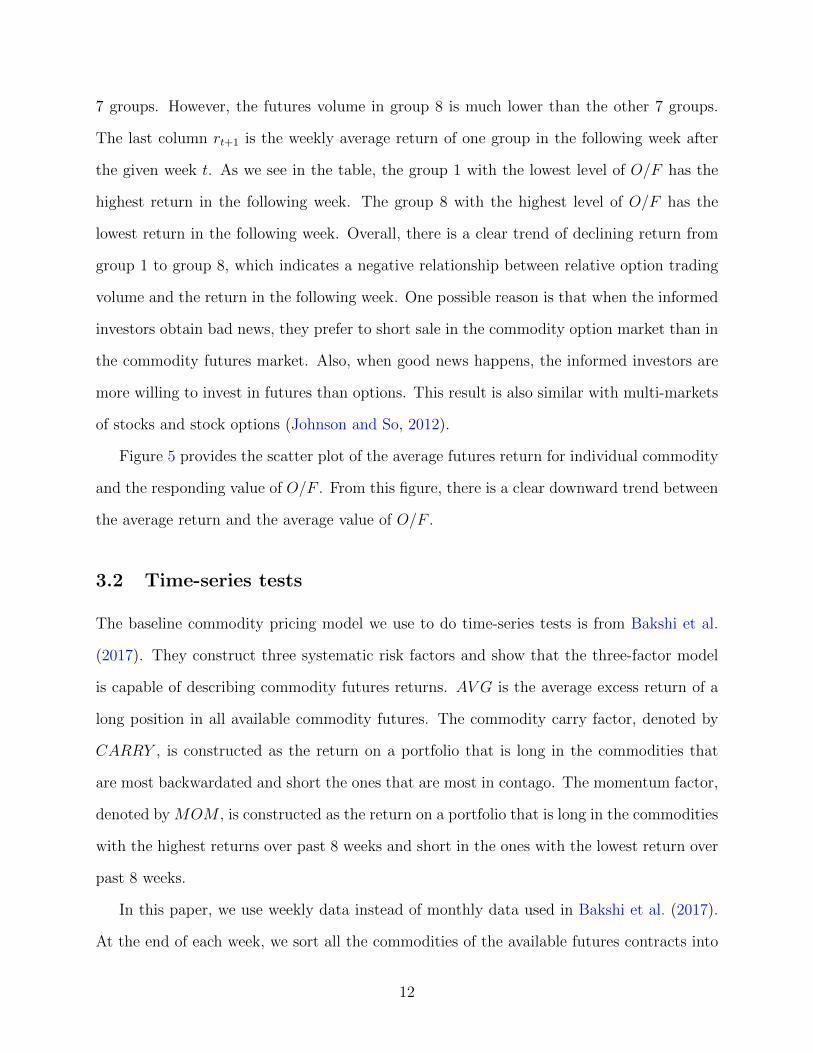
Figure 5 provides the scatter plot of the average futures return for individual commodity

and the responding value of O/F . From this figure, there is a clear downward trend between

the average return and the average value of O/F .

3.2 Time-series tests

The baseline commodity pricing model we use to do time-series tests is from Bakshi et al.

(2017). They construct three systematic risk factors and show that the three-factor model

is capable of describing commodity futures returns. AV G is the average excess return of a

long position in all available commodity futures. The commodity carry factor, denoted by

CARRY , is constructed as the return on a portfolio that is long in the commodities that

are most backwardated and short the ones that are most in contago. The momentum factor,

denoted by MOM , is constructed as the return on a portfolio that is long in the commodities

with the highest returns over past 8 weeks and short in the ones with the lowest return over

past 8 weeks.

In this paper, we use weekly data instead of monthly data used in Bakshi et al. (2017).

At the end of each week, we sort all the commodities of the available futures contracts into

12

8 groups based on the level O/F . The weekly return for each group is calculated as the

equal-weighted return for a portfolio of all commodities in that group in the following week.

We compute the weekly return from the close of markets on Tuesday to the close of markets

on Tuesday in the next week.

The baseline three-factor asset pricing model of expected return representation for each

group i = 1, 2, ..., 8:

ri,t+1 = αi + β1AV Gi,t+1 + β2CARRYi,t+1 + β3MOMi,t+1 + εi,t+1

implying that the expected excess return are a function of exposure to three factors.

For each commodity, for a given week t, let F(0)t be the price of front-month futures

contract, and let F(1)t be the price of the next maturity futures contract. We define the

weekly basis for commodity i on a given week t as the log difference between the front-

month futures price and the next maturity futures price as:

Bi,t = log(F

(1)t

F(0)t

)

A commodity is in backwardation if its futures curve is downward sloping (the basis is

positive). Otherwise, the commodity is in contango.

To construct CARRY factor, we first sort available commodities by basis at the end of

week t and split them into 4 portfolios. In the following week t + 1, the futures contracts

of these commodities are one week closer to their maturities. Then we compute the weekly

return of these futures contracts in week t + 1. In each portfolio, we use equal weights to

compute the average weekly excess return of a portfolio in week t+1. The CARRY factor is

constructed using the strategy of longing the highest basis portfolio and shorting the lowest

basis portfolio.

To construct MOM factor, at the end of week t, we focus on equal weights and ranking

13

of a commodity is determined by a commodity’s past 8 weeks performance:

rt = (7∏

j=0

(1 + rt−j))18 − 1

The weekly return of a commodity is calculated as the average weekly return of all available

futures contracts for that commodity. We first sort available commodities by past perfor-

mance at the end of week t and split them into 6 portfolios. In the following week t + 1,

the futures contracts of these commodities are one week closer to their maturities. Then we

compute the average weekly return of these futures contracts in week t+1. In each portfolio,

we use equal weights to compute the weekly excess return of a portfolio in week t+ 1. The

MOM factor is computed as the strategy of longing the best performance portfolio and

shorting the worst performance portfolios.

To construct the AV G factor, we aggregate the excess returns of all available futures

contracts using equal weights to calculate the average market return for each week t.

Table 4 presents the time-series factor regression for each group using three regressions.

The first regression we use is the commodity CAPM, the intercept for each group tends to

decrease with O/F . We find that the commodity portfolio with lowest O/F has the highest

alpha of 0.001 (t-statistic = 2.732). And the portfolio of commodity with highest O/F has

the lowest alpha of -0.001 (t-statistic = -2.275). The “1-8” column takes a statistical test for

the difference of lowest between highest portfolios, the results show that there is a positive

and significant difference (t-statistic = 3.144). The ”(1+2)-(7+8)” takes a statistical test for

the difference of two lowest and two highest O/F portfolios, we find that there is a positive

and significant difference (t-statistic = 2.244).

The second regression employed is commodity AV G and CARRY . The third regression

contains all the three factors. In these two regressions, the lowest O/F portfolio has the

highest statistically significant alpha and the highest O/F portfolio has the lowest statisti-

cally significant alpha. For the columns ”1-8” and ”(1+2)-(7+8)”, the results are similar in

14

both magnitude and statistical with commodity CAPM.

In summary, with the time-series tests, we find that low O/F can indicate high expected

returns. A portfolio of commodities with lowest O/F has significantly positive alpha in the

next week after portfolio formation. Also, high O/F indicates low expected returns, as the

portfolio of commodities with highest O/F has significantly negative alpha in the next week

after portfolio formation.

From table 4, we also find that the strategies of ”1-8” and ”(1+2)-(7+8)” have a signif-

icantly positive loading on the market (AV G) factor. These results indicate that low O/F

commodities have more market exposure than high O/F commodities, which is the opposite

of the result in stock market that high option to stock volume ratio firm have more market

exposure Johnson and So (2012).

3.3 Cross-sectional tests

The cross-sectional tests can be more powerful than traditional time-series tests since the

variation in O/F across different commodities at a point in time may be more informative

than the variation in O/F .

One potential concern when using the Fama-MacBeth approach is the independence in

the time dimension. The average first-order autocorrelation of weekly time-series return of

all 25 commodity futures markets is only 0.003. Based on this low autocorrelation of time

series returns, we can be confident that the independence in the time dimension is a plausible

assumption.

In addition to time-series tests, we also apply the Fama-MacBeth two-stage regression

method (Cochrane, 2009). Fama and MacBeth (1973) suggest a computationally simple

procedure for running cross-sectional regressions, and for producing standard errors and test

statistics.

The Fama-MacBeth two-stage regression method tests the hypothesis that cross-sectional

differences in asset returns are due to cross-sectional differences in asset risk exposure. The

15

Fama-MacBeth regression has two steps. First, we regress the time-series of the excess return

of commodity i on factors to estimate the vector of risk exposure (βi) as

Ri,t+1 = ai + β′

ift + εi,t, t = 1, 2, ..., T for each i

where ft is a set of risk factors. Second, we run the cross-sectional regression at each time

period t as

Ri,t+1 = γt + β′

iλt + αi,t, i = 1, 2, ..., N for each t

We estimate λ as the average of the cross-sectional regression estimates as

λ =1

T

T∑t=1

λt

In the Fama-MacBeth regressions, we include 7 factors to explain the dependent variable

RET(1): log(O/F ), CAR, MOM , AMI, RET (0), log(FV OL), log(OPV OL).

RET(1) is the dependent variable indicating the return of commodity i in week t + 1

after observing O/F at the end of week t.

log(O/F ) is the log value of O/F for commodity i in week t. CAR equals the basis of

commodity i at the end of week t. MOM is the cumulative returns measures over the past 8

weeks and adjusted by market return. RET (0) is the contemporaneous return of commodity

i in week t. log(FV OL) and log(OPV OL) equal the log value of futures and options trading

volume of commodity i in week t.

We also include the liquidity factor AMI. According to Marshall et al. (2011), the

Amihud (2002) liquidity factor is the best low-frequency liquidity measure for commodity

futures. In this paper, we use this measure for the individual futures contract liquidity. The

proxy measures absolute price changes per futures contract volume:

AMI =|rt|

V olumet

16

where rt is the return on day t and V olumet is the futures volume on day t.

Estimation results of the Fama-MacBeth regressions are reported in table 5. Column 1

contains the results of regressing RET (1) on CAR and MOM . The coefficient of MOM is

positive but not significant. The positive momentum effect doesn’t exists in the commodity

futures market for weekly data. Also, the CAR coefficient is positive but not significant,

indicating that the carry effect is not significant in the commodity market of weekly obser-

vations.

Column 2 contains one more factor AMI than column 1. Results show that liquidity does

not play an important role in predicting the weekly returns in commodity futures market.

Columns 3 and 4 contain the results of regressing RET (1) on futures volume and options

volume after controlling for carry, momentum and liquidity factors. We find that neither

futures volume nor options volume are significant in predicting futures returns, although the

coefficients of futures volume and options volume are positive and negative.

Column 5 has the result of regressing RET (1) on log(O/F ) after controlling for carry,

momentum. The result shows that log(O/F ) is negative and statistically significant at the

5% percent level.

In column 6, we also use liquidity factor besides carry and momentum as the control

variable. The variable log(O/F ) is still negative and significant (t-statistics = -2.542).

Finally, in column 7, we include the contemporaneous return in the portfolio formation

week, RET (0), to control for the possibility of weekly return reversals. Although the coeffi-

cient of RET (0) is positive, this factor is not statistically significant. Also, log(O/F ) is still

negatively significant in this regression.

In conclusion, table 5 show that the negative relation between O/F and RET (1) is robust

after controlling for the other 4 variables.

17

4 WASDE announcement analysis

In every month, United States Department of Agriculture (USDA) publishes the monthly

WASDE (World Agricultural Supply and Demand Estimates) reports to announce current

and expected market conditions for several agricultural commodities to participants in com-

modity markets. One important forecast from WASDE is the expected ending stock in end

of each marketing year. Ending stocks, also referred as carryout, are the amount of a com-

modity left over after all demand has been satisfied and enters the supply side of the market

in the following marketing year. Low ending stocks can lead to high prices of the commodity

since it is a signal for less supply of commodity.

In the previous literature, many papers have found the commodity futures react to

WASDE announcements. For instance, Adjemian (2012) analyzes the absolute value of

overnight return before and after the announcement date and confirms that the WASDE

announcement effect persists across contract positions.

This section, however, focuses on a different dimension of WASDE announcement ef-

fect. We study the link between the activities in futures and options markets and post-

announcement returns. The commodities we analyze in this section are Soybean Oil, Corn,

Cotton, Soybeans, Sugar, Soybean Meal, and Wheat.

4.1 Post-announcement returns

Our paper examines the predictive power of O/F for cumulative returns following the an-

nouncement. We use four return windows: CUM(+0,+5), CUM(+0,+10), CUM(+0,+15),

CUM(+0,+20). CUM(X,Y) equals the cumulative return for each commodity from X trading

days to Y trading days after the announcement date.

The forecast of ending stock from the WASDE report for commodity i in month m is

defined as ESi,m. To capture the news released at the announcement, the surprise of the

18

forecast in ending stocks comparing with that in the last month is constructed as:

∆ESi,m =ESi,m − ESi,m−1

ESi,m−1

The pre-announcement returns may have a significant effect on the post-announcement

returns since the informed traders can obtain private information before the announcement

and start to trade in the same direction with the results from the announcement reports.

Motivated by this rationale, we construct two more variables: pre-CUM denotes cumulative

return over the pre-announcement window (days -5 to -1); abs(pre-CUM) denotes absolute

value of cumulative return over the pre-announcement window (days -5 to -1). In the em-

pirical method, the control variables are CAR and AMI that are the basis and measure

for illiquidity for commodity over the pre-announcement window (days -5 to -1). To correct

for cross-sectional correlation, the standard errors are clustered (by time), refer to Petersen

(2009).

Table 6 presents the results about the predictive power of O/F on the cumulative returns

after announcement. In the column of CUM(+0,+5), the coefficient on ∆ES is significantly

negative (t-statstic = -4.01). Higher prediction of ending stocks for a commodity i is a

negative signal for futures price. The reason is that higher ending stocks means the sup-

ply is higher than expected, which would cause the futures price going down. After the

WASDE report is released, the participants in the commodity market obtain the new in-

formation about the predicted ending stocks and change their trading behaviors, which will

cause the decrease of futures prices 5. So the negative relation between the change in fore-

casts of ending stocks and post-announcement returns is not surprising. However, when

the horizon for cumulative returns is longer than CUM(+0,+5) such as CUM(+0,+10),

CUM(+0,+15) and CUM(+0,+20), ∆ES does not have enough predictive power for cumu-

lative post-announcement returns. So after 5 days post-announcement windows (day 0 to

day +5), the information of ending stocks from the WASDE report is not a reliable factor to

5See Appendix A for details

19

predict the futures prices over a long time period. New information will come to investors

several days after the WASDE report is released, they will make investment decisions based

on the new information, which will affect the predictive power of ∆ES.

From table 6, we find that O/F has predictive power over a longer horizon than ∆ES

does. Consistent with the results in the previous section, the coefficient of O/F is strongly

negative (t-statistics = -3.276) in the column of CUM(+0,+5). When the informed traders

obtain the private information before the announcement, they will make decisions about

investment before the report is released, which cause the significant change in options and

futures trading volume. What’s more, the coefficients of O/F are significant negative (t-

statistics = -3.171, -3.822, -3.778) for other three columns of CUM(+0,+10), CUM(+0,+15),

and CUM(+0,+20). Since the trading volume of options and futures in pre-announcement

(day -5 to day -1) not only contain the information about the WASDE report, but also

include news that is farther away than post-announcement window (day 0 to day +5). So

O/F has longer horizon in predictive power than the change of predictions in ending stocks

∆ES. The variable pre-CUM is positive and significant (t-statistics = 2.090, 1.814, 1.693)

in the columns of CUM(+0,+5), CUM(+0,+10), and CUM(+0,+15). This indicates the

momentum effect exists in before and after the announcement. The momentum effect fades

away as the time horizon becomes longer.

5 COT report analysis

5.1 Basic information about COT reports

A database commonly used in the studies of commodity market is the weekly Commitments

of Traders (COT) reports published by Commodity Futures Trading Commission (CFTC).

The COT reports include the aggregate long and short positions of commodity futures market

participants by trader type: commercials, non-commercials, and non-reportables. The COT

reports provide a breakdown of each Tuesday’s open interest for markets in which 20 or

20

more traders hold positions equal to or above the reporting levels established by the CFTC.

The weekly reports for Futures-Only Commitments of Traders and for Futures-and-Options-

Combined Commitments of Traders are released every Friday.

For the Futures-and-Options-Combined report, the option open interest and traders’

option positions are computed on a futures-equivalent basis using delta factors supplied

by the exchanges. Long-call and short-put open interest are converted to long futures-

equivalent open interest. Likewise, short-call and long-put open interest are converted to

short futures-equivalent open interest. For example, if an investor holds a long call position

of 100 contracts with the value of delta being 0.5, this trader is considered to be holding 50

contracts of long futures equivalent positions. A trader’s long and short futures-equivalent

positions are added to the trader’s long and short futures positions to give “combined-long”

and “combined-short” positions.

Each individual trader is distinguished by CFTC about whether she has a commercial

interest in each commodity. If a trader uses futures contracts in a particular commodity

for hedging as defined in CFTC Regulation 1.3, 17 CFR 1.3(z), this trader is classified as

commercial. The commercials are often considered to have long positions in the physical

product, such as corn producers, trying to reduce the risk by taking short positions in the

futures market. The non-commercials, sometimes called speculators, have no innate position

in the physical commodity, and seek to earn a profit in the futures market by taking long or

short positions to take advantage of what they view as favorable prices.

Since the COT reports only include the commodities that are traded on four American

exchanges (NYMEX, NYBOT, CBOT, and CME), we exclude Cocoa futures from ICE

London and Crude oil Brent futures from ICE Europe. In this section, the data sample

include 23 commodities and the sample period is from April 1995 to December 2018. Then

we merge the COT reports with the data of futures contracts for individual commodities.

21

5.2 Baseline model

In the previous section, we have shown that there is a negative relation between the option-

to-futures volume ratio and futures returns in the next week. The results indicate that the

informed traders tend to trade in commodity option markets instead of futures market when

hear bad news. Since the main participants in commodity markets are commercials and

non-commercials (speculators), it is meaningful to investigate the behaviors of these two

type traders.

Kang et al. (2017) also use weekly data (futures returns are constructed as Tuesday-

Tuesday) to study the dynamic interaction between the net positions and risk premiums in

commodity futures markets. For the short-term horizon (weekly level), the position changes

are mainly driven by the liquidity demands of non-commercial traders. Also, we calculate the

weekly return for each futures contract with different maturity for each commodity. However,

Kang et al. (2017) compute the weekly excess return using the front-month contract. Since

the open interest of COT reports is the total of all futures and option contracts for each

commodity, our data sample is more consistent with the data in the COT reports.

We use the main model from Kang et al. (2017) as our baseline model. In their paper, they

construct three variables to characterize the positions and trading behavior of participants

in futures markets: hedging pressure (HP ), net trading (Q), and the propensity to trade

(PT ).

Hedging pressure (HP ) is defined as the number of contracts that the commercial traders

are short minus the number of contracts that are long, divided by the total open interest.

For commodity i in week t:

HPi,t =commercial netshort positionsi,t

OIi,t

HP i,t is calculated as trailing 52-week moving average of the net short positions of com-

mercials from week t− 51 to week t scaled by the open interest in week t. Kang et al. (2017)

22

show that HP i,t captures sources of variation in risk premiums and significantly predicts

expected returns.

For commercials and non-commercials, the net trading measure (Q) is defined as the net

purchase of futures contracts, calculated as the change in their long position for commodity

i from week t− 1 to week t, normalized by the open interest at the beginning of the week:

Qi,t =netlong positioni,t − netlong positioni,t−1

OIi,t−1

Column 1 in table 7 shows the results of the baseline model for commercials and confirms

the findings by Kang et al. (2017). The commodities that are bought by the commercials in

week t earn significant higher returns in week t+ 1 than the commodities sold by them. The

coefficient of HP is also positive and similar with Kang et al. (2017), although not statistical

significant. The results of the baseline model for non-commercials are in column 3 of table

7. The results in column 3 also replicate the results from Kang et al. (2017). The variable

HP is significant to predict the risk premium of commodity in the multivariate regression.

One concern is that whether the relationship between O/F and the expected returns still

hold in this baseline model. Table 7 helps to address this concern. In the regressions for

commercials and non-commercials in columns 2 and 4, the coefficients of log(O/F ) remain

significant at 1% level (t-statistics = -2.614 and -3.142). These estimates indicate strong

support for the findings in the previous section.

5.3 Liquidity supply and demand in commodity options market

An intuitive extension of Kang et al. (2017) is to explore the liquidity supply and demand

in commodity options market. Our empirical strategy in this section parallels the empirical

method in Kang et al. (2017) for commodity futures market. In commodity options market,

we construct net trading measure (NT ) as the net purchase of options contracts for com-

mercials and non-commercials, calculated as the change in their net long position in options

23

contracts for commodity i from week t− 1 to week t, normalized by the open interest at the

beginning of the week:

NTi,t =netlong positioni,t − netlong positioni,t−1

OIi,t−1

where OIi,t−1 is the total open interest (including futures and options) at week t− 1.

We first explore the relationship between the net trading measure (NT ) in options and

contemporaneous or past returns. The average first-order autocorrelation of weekly time-

series NT of all 23 commodity futures markets for commercials and non-commercials are only

-0.056 and -0.036. Based on this low autocorrelation of time series NT , we can be confident

to employ the Fama-MacBeth regression. Table 8 presents the time series average of the slope

coefficients and the corresponding t-statistics. For both commercials and non-commercials,

the net trading measure (NT ) is significantly correlated to the contemporaneous and lagged

commodity futures returns. However, the correlations between net trading measure (NT )

in options with returns have opposite signs for commercials (negative) and non-commercials

(positive). Actually, the commercials are contrarians and non-commercials are momentum

traders in commodity options market. These results are consistent with the findings in Kang

et al. (2017) in commodity futures market, as well as the results in Rouwenhorst and Tang

(2012).

Motivated by the models in Campbell et al. (1993), Grossman and Miller (1988), Kaniel

et al. (2008) and Kang et al. (2017), the market makers typically trade against price trends

and are compensated for providing liquidity by the price reversal subsequently. To deter-

mine the direction of liquidity provision, we conduct the analysis about the impact of net

trading measure (NT ) in options on the subsequent commodity futures returns. We run the

predictive Fama-MacBeth regressions of cumulative commodity futures returns from week t

to weeks t+ 1, t+ 2, and t+ 3 on the net trading measure (NT ) in options with the control

24

variables to capture variation in expected futures returns:

RET(t,t+j)i = αi + β1NTi,t + β2CARi,t + β3ri,t + β4Qi,t + β5HP i,t + εi,t+j, j = 1, 2, 3

where RET(t,t+j)i is the cumulative return of commodity i from week t to t + j. CARi,t is

the log of basis for commodity i in week t, HP i,t is the moving average of hedging pressure

for commodity i in week t.

From table 9, we find that the commodities bought by the commercials in week t has

significant higher cumulative returns in the subsequent three weeks than the commodities

sold by the commercials after controlling other variables. However, from table 10, the com-

modities bought by the non-commercials in week t has significant lower cumulative returns

in the subsequent three weeks than the commodities sold by the non-commercials.

One concern is that the commercials have the private information so the prices of com-

modities they buy have higher chance to increase in the subsequent time periods. The com-

mercials have the information advantage in the underlying physical commodities markets

that is about the the fundamentals in the commodity markets, which the non-commercials

may not be able to observe. If the commercial traders have the private information in

commodity market, the price of commodities purchased by the commercials should simulta-

neously increase (Kang et al., 2017). However, in table 8, the commercials are buying losers

and sell winner before the release of the COT report, which is consistent with the theory of

liquidity provision.

Overall, we find the clear answer for the question which participant provide the liquidity

in commodity options markets. The empirical results show that, in the commodity options

market, the commercials buy losers, sell winners, employ the contrarian strategy and provide

the liquidity to satisfy the trading demand of non-commercial traders.

25

6 Robustness checks

6.1 Before and after the start of financialization

In the most recent decade, commodity index traders have become a significant big player in

the commodity market. This fundamental change is called the financialization of commodity

markets. Referring to figure 3, there is a sharp decline of O/F since year 2005, which

confirms the existence of financialization in commodity markets. Because commodity index

traders mainly invest in the futures market, O/F fell sharply since year 2005. So it has

great importance to investigate whether the empirical results would change before and after

the start of financializtion in commodity market. We divide the whole sample interval into

two sub-periods. Sub-period 1 include the time period before year 2005 (including 2005);

sub-period 2 is the time period after year 2005.

First, we employ time-series tests for these two sub-periods. The baseline model is the

same as that in Section 3.2. The results for the time-series tests are in table B.1 and table

B.2. For sub-period 1, the “1-8” and “(1+2)-(7+8)” columns show positive significant alpha

for one, two, three factor models. Column 1 also presents positive significant alpha (t-

statistics = 2.277, 2.451, 2.331) for all three models. For sub-period 2, all the alphas are

positive significant in column 1 and ”1-8” for all the models. In summary, the results in two

sub-periods pass the time-series tests.

Next, the cross-sectional tests are conducted for both sub-periods as in Section 3.3. From

table B.3, the coefficients of O/F are negative significant in both models for the two sub-

periods.

6.2 Commodity sector analysis

Do our results hold in different sectors, or are they mainly driven by one sector of commodities

that have high expected returns with low O/F or low expected returns with high O/F? We

sort our sample commodities into 4 sectors: Agriculture, Energy, Livestock, and Metals. For

26

each sector, the cross-sectional tests are employed. In table B.4, we report the results for each

sector. The predictive power of O/F still exists and negatively significant in Agriculture,

Energy, and Livestock sectors. An interesting finding is that the impact of CAR, MOM

and AMI is different from table 5, which is based on the whole sample. CAR and MOM

have opposite significant impact in predicting prices, then it is not surprised that these two

variables are not significant in the cross-sectional results based on the whole sample.

6.3 Monthly analysis

In the previous sections of our paper, we use the weekly data to do the analysis. In the

literature, many papers use the monthly data such as Yang (2013), Bakshi et al. (2017), and

Hong and Yogo (2012). An intuitive question is to ask whether the empirical results only

hold in the weekly data. In this section, we assess whether we can get similar results in

monthly data.

The results of monthly analysis are reported in table B.5. The coefficient of O/F remains

positively significant after controlling different variables, which indicates O/F has good

predictive power even on a longer long time period.

6.4 Alternative measure ∆O/F

The last robustness check is to utilize an alternative measure of O/F . Similar to the stock

market, one potential concern with our empirical results is that some commodities could

have consistently higher O/F and lower average returns for some reasons (Johnson and So,

2012). To address this concern, we construct an alternative measure ∆O/F as the change in

O/F relative to a rolling average of past O/F in prior 8 weeks for each commodity. ∆O/F

is defined as:

∆O/Fi,t =O/Fi,t −O/Fi

O/Fi

where O/Fi is the average O/Fi,t for commodity i over the prior 8 weeks.

27

The results in table B.6 show that the coefficient estimates of ∆O/F are negative and

significant, which is consistent with our expectation. We can address the concern that some

commodities have consistently high O/F with low average returns or low O/F with high

average returns.

7 Conclusion

In this paper, we examine the information content in commodity futures and options volume.

In the previous literature, commodity options markets have received much less attention

than commodity futures markets. However, the trading activities in options markets can

have great effect on the underlying futures markets. We are the first to study the option-to-

futures volume ratio in an empirical asset pricing framework.

After the time-series tests and cross-sectional tests, we confirm the return predictability

of O/F . Our results are robust across a variety of specifications. Our paper makes an unique

contribution to confirm WASDE announcement effect. Comparing with the predictive ability

of the information contained in WASDE report, O/F has relatively long-lived predictive

power, which suggests that it takes multiple weeks for the information in O/F to become fully

reflected in futures prices. In the analysis of COT reports, we find that the non-commercial

traders in commodity options markets demand short-term liquidity from the commercial

traders. Non-commercials pay a premium by buying the underperformance commodities

and sell outperformance commodities.

Our work suggests many areas of further research. First, given the data of commodity

options, an interesting topic is to explore the determinants of volatility in commodity futures

prices since the investors often refer to implied volatility to make investment decisions on

options market. Second, the volume differences across calls and puts could be examined to

predict commodity futures returns skewness, which can be a good complement to Fernandez-

Perez et al. (2018). Finally, a critically important topic is to find more empirical evidence

28

to explain why there is a negative and significant relationship between O/F and expected

futures returns. These and other issues are left for future research.

29

References

Acharya, V. V., L. A. Lochstoer, and T. Ramadorai (2013). Limits to arbitrage and hedging:

Evidence from commodity markets. Journal of Financial Economics 109 (2), 441–465.

Adjemian, M. K. (2012). Quantifying the wasde announcement effect. American Journal of

Agricultural Economics 94 (1), 238–256.

Amihud, Y. (2002). Illiquidity and stock returns: cross-section and time-series effects. Jour-

nal of financial markets 5 (1), 31–56.

An, B.-J., A. Ang, T. G. Bali, and N. Cakici (2014). The joint cross section of stocks and

options. The Journal of Finance 69 (5), 2279–2337.

Baker, S. D. (2014). The financialization of storable commodities.

Bakshi, G., X. Gao, and A. G. Rossi (2017). Understanding the sources of risk underlying

the cross section of commodity returns. Management Science.

Basak, S. and A. Pavlova (2016). A model of financialization of commodities. The Journal

of Finance 71 (4), 1511–1556.

Basu, D. and J. Miffre (2013). Capturing the risk premium of commodity futures: The role

of hedging pressure. Journal of Banking & Finance 37 (7), 2652–2664.

Brunetti, C. and D. Reiffen (2014). Commodity index trading and hedging costs. Journal

of Financial Markets 21, 153–180.

Campbell, J. Y., S. J. Grossman, and J. Wang (1993). Trading volume and serial correlation

in stock returns. The Quarterly Journal of Economics 108 (4), 905–939.

Chan, K., L. Ge, and T.-C. Lin (2015). Informational content of options trading on acquirer

announcement return. Journal of Financial and Quantitative Analysis 50 (5), 1057–1082.

30

Cheng, I.-H., A. Kirilenko, and W. Xiong (2014). Convective risk flows in commodity futures

markets. Review of Finance 19 (5), 1733–1781.

Cochrane, J. H. (2009). Asset pricing: Revised edition. Princeton university press.

Cremers, M. and D. Weinbaum (2010). Deviations from put-call parity and stock return

predictability. Journal of Financial and Quantitative Analysis 45 (2), 335–367.

Daskalaki, C., A. Kostakis, and G. Skiadopoulos (2014). Are there common factors in

individual commodity futures returns? Journal of Banking & Finance 40, 346–363.

Domanski, D. and A. Heath (2007). Financial investors and commodity markets. BIS

Quarterly Review , 53.

Easley, D., S. Hvidkjaer, and M. O’hara (2002). Is information risk a determinant of asset

returns? The journal of finance 57 (5), 2185–2221.

Fama, E. F. and J. D. MacBeth (1973). Risk, return, and equilibrium: Empirical tests.

Journal of political economy 81 (3), 607–636.

Fernandez-Perez, A., B. Frijns, A.-M. Fuertes, and J. Miffre (2018). The skewness of com-

modity futures returns. Journal of Banking & Finance 86, 143–158.

Ge, L., T.-C. Lin, and N. D. Pearson (2016). Why does the option to stock volume ratio

predict stock returns? Journal of Financial Economics 120 (3), 601–622.

Goldstein, I. and L. Yang (2017). Commodity financialization and information transmission.

Gorton, G. B., F. Hayashi, and K. G. Rouwenhorst (2012). The fundamentals of commodity

futures returns. Review of Finance 17 (1), 35–105.

Grossman, S. J. and M. H. Miller (1988). Liquidity and market structure. the Journal of

Finance 43 (3), 617–633.

31

Hong, H. and M. Yogo (2012). What does futures market interest tell us about the macroe-

conomy and asset prices? Journal of Financial Economics 105 (3), 473–490.

Hu, J. (2014). Does option trading convey stock price information? Journal of Financial

Economics 111 (3), 625–645.

Jagannathan, R. (1985). An investigation of commodity futures prices using the

consumption-based intertemporal capital asset pricing model. The Journal of Fi-

nance 40 (1), 175–191.

Johnson, T. L. and E. C. So (2012). The option to stock volume ratio and future returns.

Journal of Financial Economics 106 (2), 262–286.

Johnson, T. L. and E. C. So (2017). A simple multimarket measure of information asymme-

try. Management Science 64 (3), 1055–1080.

Kacperczyk, M. T. and E. Pagnotta (2018). Chasing private information.

Kang, W., K. G. Rouwenhorst, and K. Tang (2017). A tale of two premiums: The role

of hedgers and speculators in commodity futures markets. Yale International Center for

Finance Working Paper (14-24).

Kaniel, R., G. Saar, and S. Titman (2008). Individual investor trading and stock returns.

The Journal of Finance 63 (1), 273–310.

Keynes, J. M. (1930). A treatise on money: in 2 volumes. Macmillan & Company.

Marshall, B. R., N. H. Nguyen, and N. Visaltanachoti (2011). Commodity liquidity mea-

surement and transaction costs. The Review of Financial Studies 25 (2), 599–638.

Miffre, J., A.-M. Fuertes, and A. Fernandez-Perez (2012). Commodity futures returns and

idiosyncratic volatility. Available at SSRN .

32

Petersen, M. A. (2009). Estimating standard errors in finance panel data sets: Comparing

approaches. The Review of Financial Studies 22 (1), 435–480.

Roll, R., E. Schwartz, and A. Subrahmanyam (2010). O/s: The relative trading activity in

options and stock. Journal of Financial Economics 96 (1), 1–17.

Rouwenhorst, K. G. and K. Tang (2012). Commodity investing. Annu. Rev. Financ.

Econ. 4 (1), 447–467.

Singleton, K. J. (2013). Investor flows and the 2008 boom/bust in oil prices. Management

Science 60 (2), 300–318.

Smith, A. (2005). Partially overlapping time series: A new model for volatility dynamics in

commodity futures. Journal of Applied Econometrics 20 (3), 405–422.

Sockin, M. and W. Xiong (2015). Informational frictions and commodity markets. The

Journal of Finance 70 (5), 2063–2098.

Stilger, P. S., A. Kostakis, and S.-H. Poon (2016). What does risk-neutral skewness tell us

about future stock returns? Management Science 63 (6), 1814–1834.

Szymanowska, M., F. De Roon, T. Nijman, and R. Van den Goorbergh (2014). An anatomy

of commodity futures risk premia. The Journal of Finance 69 (1), 453–482.

Tang, K. and W. Xiong (2012). Index investment and the financialization of commodities.

Financial Analysts Journal 68 (5), 54–74.

Working, H. (1960). Speculation on hedging markets. Food Research Institute Stud-

ies 1 (1387-2016-116000), 185.

Yang, F. (2013). Investment shocks and the commodity basis spread. Journal of Financial

Economics 110 (1), 164–184.

33

Figure 1: Procedure to select sample

34

0

100

200

300

400

1994 1996 1998 2000 2002 2004 2006 2008 2010 2012 2014 2016 2018

Year

Trad

ing

volu

me

(*10

^3)

Futures_Volume Options_Volume

Figure 2: Options and futures volume by year from 1994 to 2018

35

0.15

0.20

0.25

0.30

1994 1996 1998 2000 2002 2004 2006 2008 2010 2012 2014 2016 2018

Year

O/F

Figure 3: Average annual value of O/F between 1994 to 2018

0.15

0.20

0.25

0.30

1994 1996 1998 2000 2002 2004 2006 2008 2010 2012 2014 2016 2018

Year

O/F

Figure 4: Average annual value of O/F excluding gasoline futures and options between 1994to 2018

36

Soybean oil Corn

Cocoa (ICE−US)

CottonOrange juice

Coffee

Lumber

Oats

Cocoa (ICE−London)Rough rice

Soybeans

Sugar

Soybean meal

Wheat

Crude oil (WTI)

Crude oil (Brent)

Heating oil

Natural gas

Gasoline

Feeder cattle Live cattle

Lean hogs

GoldCopper Silver

−0.4

−0.2

0.0

0.2

0.0 0.1 0.2 0.3 0.4

O/F

Ret

urn

Figure 5: Cross-sectional of average futures return and average value of O/F .

37

Table 1: Summary statistics of commodity futures for every individual commodity in thesample.

The sample include the average weekly close quotes of individual futures contract of 25 com-modities from March 1994 to December 2018. The column N is the number of weekly ob-servations available for a commodity. The column O/F reports the historical average weeklyratio of options-to-futures trading volumes. The columns E[R](%) and σ[R] are the historicalaverage and standard deviation of weekly futures excess returns of individual commodities withdifferent maturities.

Sector Commodity Symbol N O/F E[R](%) σ[R] Sharpe ratio

Agriculture Soybean oil BO 1641 0.091 -0.131 0.033 -4.021Corn C 988 0.300 -0.125 0.037 -3.354Cocoa (ICE-US) CC 1035 0.154 -0.024 0.039 -0.622Cotton CT 1015 0.400 -0.082 0.035 -2.323Orange juice JO 1232 0.291 -0.080 0.044 -1.825Coffee KC 1032 0.415 -0.121 0.051 -2.397Lumber LB 1196 0.074 -0.211 0.042 -5.033Oats O 908 0.075 0.023 0.046 0.495Cocoa (ICE-London) QC 777 0.156 -0.193 0.036 -5.310Rough rice RR 1215 0.085 -0.220 0.035 -6.339Soybeans S 1414 0.341 -0.011 0.032 -0.330Sugar SB 840 0.249 -0.221 0.043 -5.112Soybean meal SM 1633 0.106 0.112 0.036 3.076Wheat W 988 0.255 -0.223 0.041 -5.499

Energy Crude oil (WTI) CL 2548 0.196 0.025 0.047 0.532Crude oil (Brent) CO 1958 0.057 0.249 0.043 5.843Heating oil HO 2415 0.029 0.077 0.044 1.740Natural gas NG 2460 0.080 -0.411 0.062 -6.608Gasoline XB 1193 0.013 -0.071 0.047 -1.512

Livestock Feeder cattle FC 1687 0.132 0.031 0.020 1.550Live cattle LC 1176 0.199 0.040 0.021 1.856Lean hogs LH 1504 0.154 -0.063 0.036 -1.769

Metals Gold GC 1233 0.135 0.032 0.023 1.425Copper HG 1840 0.008 0.045 0.034 1.307Silver SI 1032 0.090 0.052 0.039 1.332

38

Table 2: Descriptive statistics of O/F by year.

This table provides the sample size information and descriptive of O/Fi,t,T , where O/Fi,t,T

is the ratio of option volume to futures volume of the contract with maturity T of com-modity i in each week t from March 1994 to December 2018. The column Commodities isthe number of commodities that appear in each year. The column Contracts is the totalnumber of contracts of all commodities in each year. The column N is the total numberof weekly observations of all commodities available in a year. The last 5 columns are themean, 25th percentile, median, 75th percentile and skewness of O/Fi,t,T for each year.

Year Commodities Contracts N MEAN P25 MEDIAN P75 SKEW

1994 23 139 988 0.207 0.058 0.107 0.209 9.7681995 24 193 1434 0.276 0.066 0.136 0.256 15.1931996 24 176 1295 0.259 0.083 0.163 0.303 7.9381997 24 191 1376 0.254 0.078 0.165 0.282 14.4791998 24 197 1448 0.248 0.079 0.175 0.298 5.5611999 24 199 1484 0.251 0.080 0.158 0.267 13.6862000 24 197 1432 0.326 0.066 0.149 0.266 9.6442001 23 173 1249 0.291 0.073 0.168 0.301 6.8102002 24 188 1332 0.318 0.057 0.152 0.310 13.6942003 24 196 1393 0.309 0.055 0.139 0.278 13.4102004 24 191 1334 0.286 0.061 0.166 0.339 8.5712005 24 180 1210 0.312 0.065 0.139 0.272 13.5142006 25 195 1365 0.225 0.045 0.130 0.267 24.9462007 25 197 1442 0.158 0.030 0.075 0.178 12.8952008 25 208 1456 0.169 0.034 0.079 0.194 10.0302009 25 209 1428 0.158 0.021 0.064 0.165 19.0232010 25 214 1472 0.138 0.020 0.067 0.175 5.6152011 25 213 1511 0.158 0.020 0.070 0.213 4.0872012 25 202 1477 0.205 0.029 0.079 0.223 20.2202013 25 211 1497 0.170 0.043 0.095 0.220 23.9242014 25 211 1486 0.174 0.038 0.109 0.236 11.8472015 25 213 1499 0.171 0.040 0.110 0.228 7.6502016 25 206 1457 0.164 0.041 0.105 0.225 4.4922017 25 207 1457 0.160 0.036 0.100 0.214 8.0082018 25 195 1438 0.165 0.030 0.104 0.204 12.095

ALL 25 4281 34960 0.220 0.044 0.119 0.246 19.670

39

Table 3: Group characteristics sorted by O/F .

This table provides the characteristics of groups sort by O/F for all weekly observations. The daterange of the sample is from March 1994 to December 2018. We divide the sample data into 8 groupswith the same number of commodity-weeks data. Group 1 is with the lowest value of O/F . Group8 has the highest value of O/F . The column Commodities and Contracts are the total number ofcommodities and contracts in each group. VLC and VLP are the average call and put contractstrading volume in each group. OPVOL and FVOL are the average options and futures trading volumein each group. The column O/F is historical average value of O/F for each group. rt+1 is the weeklyaverage return of a group in the next week after the given week t.

Group Commodities Contracts VLC VLP OPVOL FVOL O/F rt+1

1 21 1147 660.648 571.822 1232.470 158066.472 0.008 0.0542 23 1666 2443.777 2209.608 4653.385 147130.722 0.031 0.0153 25 1852 4710.775 4302.299 9013.074 150986.305 0.060 -0.0134 25 2022 8005.445 7323.093 15328.538 156346.984 0.097 -0.1125 25 2097 14934.845 14631.800 29566.645 204271.365 0.145 0.0186 25 1985 20693.111 19690.694 40383.805 195293.307 0.207 -0.0387 25 1791 25686.789 23791.294 49478.082 165071.331 0.303 -0.1018 24 1369 22782.214 19535.015 42317.229 77647.619 0.909 -0.220

40

Table 4: Time-series tests results of groups sorted by O/F

The groups are sorted by O/Fi,t, where O/Fi,t is the ratio of option volume to futures volume of commodity i in week t. Group 1has the lowest value of O/F , where group 8 is with highest O/F . The return of each group is the weekly return in week t+ 1. Weinclude three contemporaneous risk factors of week t + 1 in the regressions: AV G, CARRY , MOM . The three regressions havepart or full of these three risk factors. The t-statistics are shown in parenthesis.

1 (Low) 2 3 4 5 6 7 8 (High) 1-8 (1+2)-(7+8)

Commodity CAPM

Alpha 0.001 -0.0002 0.0004 -0.001 -0.001 0.0003 -0.0002 -0.001 0.003 0.003(2.732) (-0.343) (0.702) (-1.438) (-1.063) (0.540) (-0.361) (-2.275) (3.144) (2.244)

AV G 1.137 0.862 0.831 0.739 0.728 0.905 0.951 0.875 0.263 0.173(42.188) (28.158) (26.196) (24.978) (22.547) (27.928) (29.173) (26.336) (5.530) (2.583)

R2 0.580 0.381 0.347 0.326 0.283 0.377 0.398 0.350 0.022 0.004

Commodity AV G and CARRY

Alpha 0.001 -0.0001 0.001 -0.001 -0.001 0.0003 -0.0003 -0.001 0.003 0.003(2.809) (-0.170) (0.820) (-1.542) (-1.061) (0.544) (-0.400) (-2.246) (3.164) (2.360)

AV G 1.141 0.869 0.835 0.735 0.728 0.905 0.951 0.876 0.264 0.182(42.228) (28.446) (26.286) (24.812) (22.473) (27.913) (29.116) (26.299) (5.546) (2.713)

CARRY -0.036 -0.055 -0.014 0.030 -0.007 -0.030 -0.006 -0.014 -0.022 -0.071(-2.043) (-2.794) (-0.666) (1.599) (-0.332) (-1.423) (-0.291) (-0.633) (-0.716) (-1.637)

R2 0.581 0.386 0.349 0.326 0.282 0.377 0.397 0.349 0.022 0.006

Commodity AV G, CARRY and MOM

Alpha 0.002 -0.0001 0.0005 -0.001 -0.001 0.0004 -0.0002 -0.002 0.003 0.003(2.869) (-0.164) (0.742) (-1.647) (-1.106) (0.661) (-0.377) (-2.341) (3.267) (2.423)

AV G 1.138 0.869 0.838 0.740 0.731 0.899 0.950 0.881 0.256 0.175(41.996) (28.331) (26.334) (24.925) (22.471) (27.680) (28.975) (26.388) (5.371) (2.602)

CARRY -0.033 -0.055 -0.018 0.025 -0.009 -0.023 -0.005 -0.019 -0.014 -0.063(-1.862) (-2.751) (-0.861) (1.315) (-0.450) (-1.111) (-0.231) (-0.876) (-0.444) (-1.454)

MOM -0.021 -0.002 0.030 0.038 0.018 -0.046 -0.009 0.039 -0.059 -0.053(-1.220) (-0.128) (1.500) (2.033) (0.901) (-2.257) (-0.434) (1.859) (-1.994) (-1.259)

R2 0.581 0.386 0.350 0.328 0.281 0.379 0.397 0.351 0.024 0.006

41

Table 5: Cross-sectional tests results

This table presents Fama-MacBeth regression results from regressing RET (1) on risk factors.RET (1) is the dependent variable indicates the return of commodity i in week t + 1 afterobserving O/F at the end of week t. CAR equals the basis of commodity i at the end of week t.MOM is the cumulative returns measures over the past 8 weeks and adjusted by market return.AMI is the Amihud illiquidity of commodity i in week t. RET (0) is the contemporaneousreturn of commodity i in week t. FV OL equals the futures volume of commodity i in week t.OPV OL equals the options volume of commodity i in week t. The t-statistics are shown inparenthesis. The notations ***, **, * indicate the coefficient is significant at the 1%, 5%, and10% level, respectively.

Fama-MacBeth regressions of RET(1)

(1) (2) (3) (4) (5) (6) (7)

CAR -0.982 -0.915 -0.582 -0.933 -0.530 -0.410 -0.479(-0.977) (-0.894) (-0.556) (-0.890) (-0.522) (-0.396) (-0.424)

MOM 0.299 0.363 0.322 0.360 0.293 0.371 0.415(0.637) (0.758) (0.672) (0.749) (0.624) (0.779) (0.789)

AMI 2.339 7.077 0.630 1.729 2.818(0.416) (0.883) (0.089) (0.299) (0.410)

log(FV OL) 0.027(1.161)

log(OPV OL) -0.016(-1.189)

log(O/F ) -0.040∗∗ -0.049∗∗ -0.067∗∗∗

(-2.161) (-2.542) (-3.307)

RET (0) 1.003(0.866)

Constant 0.952 0.882 0.280 1.054 0.406 0.267 0.307(0.937) (0.854) (0.257) (0.993) (0.395) (0.255) (0.268)

Observations 27,024 27,024 27,024 27,024 27,024 27,024 25,729R2 0.268 0.313 0.344 0.323 0.273 0.320 0.387

42

Table 6: Results for post-announcement cumulative returns analysis

This table presents the results about the predictive power of O/F on the cumulativereturns after the announcement. ∆ES is the change of forecast in ending stock from lastmonth to current month, scaled by the forecast in the last month. pre-CUM denotescumulative return over the pre-announcement window (days -5 to -1); abs(pre-CUM)denotes absolute value ofcumulative return over the pre-announcement window (days -5to -1). CAR and AMI are the basis and measure for illiquidity for commodity over thepre-announcement window. The standard errors are clusterd (by time). The t-statisticsare shown in parentheses. The notations ***, **, * indicate the coefficient is significantat the 1%, 5%, and 10% level, respectively.

Dep. variable: CUM(+0,+5) CUM(+0,+10) CUM(+0,+15) CUM(+0,+20)

∆ES −3.992∗∗∗ 0.122 0.039 0.021(−4.007) (1.093) (0.399) (0.267)

log(O/F) −0.280∗∗∗ −0.040∗∗∗ −0.043∗∗∗ −0.036∗∗∗

(−3.276) (−3.171) (−3.822) (−3.778)

pre-CUM 0.080∗∗ 0.010∗ 0.009∗ 0.007(2.090) (1.814) (1.693) (1.566)

abs(pre-CUM) −0.080 −0.007 −0.003 −0.004(−1.515) (−0.944) (−0.386) (−0.800)

CAR 7.122∗ 0.707 1.006∗∗ 0.578∗

(1.938) (1.504) (2.225) (1.652)

AMI −204.298 108.648 84.806∗ 38.321(−0.346) (1.376) (1.862) (0.645)

Constant −7.632∗∗ −0.798∗ −1.102∗∗ −0.651∗

(−2.032) (−1.649) (−2.375) (−1.810)

Observations 2,190 2,090 2,090 2,090R2 0.026 0.013 0.017 0.014

43

Table 7: Results for Commercials and Non-Commercials

This table presents Fama-MacBeth regression results from regress-ing RET (1) on risk factors for commercials and non-commercials.RET (1) is the dependent variable indicates the return of commod-ity i in week t + 1 after observing O/F at the week t. RET (0)is the return of commodity i in week t. CAR equals the basis ofcommodity i at the end of week t. Q is the net trading measureof commercials and non-commercials for commodity i in week t.HP is the smoothed hedging pressure for commodity i in week t.The t-statistics are shown in parenthesis. The notations ***, **, *indicate the coefficient is significant at the 1%, 5%, and 10% level,respectively.

Fama-MacBeth regressions of RET(1)

Commercials Non-Commercials

(1) (2) (3) (4)

CAR -0.737 -0.382 -0.977 -0.696(-0.625) (-0.311) (-0.821) (-0.567)

RET (0) 3.053∗∗ 2.209 2.883∗∗ 2.134(2.185) (1.514) (2.095) (1.503)

Q 5.460∗∗∗ 4.610∗∗∗ -6.009∗∗∗ -5.297∗∗∗

(5.048) (3.916) (-5.134) (-4.217)

HP 0.280 0.281 0.381∗ 0.389∗

(1.443) (1.400) (1.940) (1.935)

log(O/F ) -0.076∗∗∗ -0.085∗∗∗

(-2.614) (-3.142)

Constant 0.694 0.170 0.913 0.444(0.582) (0.136) (0.758) (0.356)

Observations 21,548 21,548 21,548 21,548R2 0.294 0.310 0.291 0.306

44

Table 8: Relationship of NT with contemporaneous and lagged returns

This table presents the Fama-MacBeth regression results from re-gressing NT (0) on risk factors for commercials. RET (0) is thecontemporaneous return of commodity i in week t. RET (−1) isone lag return of commodity i in week t − 1. NT (−1) is one lagnet trading measure (NT ) of commodity i in week t − 1. Thet-statistics are shown in parenthesis. The notations ***, **, * in-dicate the coefficient is significant at the 1%, 5%, and 10% level,respectively.

Dependent Variable: NT(0)

Commercial Non-Commercial

(1) (2) (3) (4)

RET (0) -0.095∗∗∗ 0.067∗∗∗

(-32.235) (26.070)

RET (−1) -0.007∗∗ 0.013∗∗∗

(-2.454) (4.800)

NT (−1) -0.003 0.023∗

(-0.205) (1.680)

Constant -0.0001∗∗ -0.0001 0.0001∗∗ 0.0001∗

(-2.000) (-1.426) (2.034) (1.671)

Observations 22,416 22,396 22,416 22,396R2 0.218 0.170 0.142 0.149

45

Table 9: Return predictability of NT for Commercials

This table presents the Fama-MacBeth regression results from regress-ing RET (1) on risk factors for commercials. RET (1) is the dependentvariable indicates the return of commodity i in week t + 1. The con-trol variables are CAR, RET (0), HP , and Q. The t-statistics areshown in parenthesis. The notations ***, **, * indicate the coefficientis significant at the 1%, 5%, and 10% level, respectively.

Return predictability for Commercials

RET(+0,+1) RET(+0,+2) RET(+0,+3)

CAR -0.828 -2.250 -1.522(-0.663) (-1.248) (-0.690)

RET (0) 3.492∗∗ 6.608∗∗∗ 8.843∗∗∗

(2.280) (3.062) (3.327)

HP 0.252 0.499∗ 0.876∗∗

(1.244) (1.701) (2.391)

Q 5.730∗∗∗ 8.604∗∗∗ 10.226∗∗∗

(4.775) (4.815) (4.699)

NT 9.815∗ 23.416∗∗∗ 23.863∗∗

(1.647) (2.902) (2.361)

Constant 0.801 2.193 1.392(0.634) (1.202) (0.624)

Observations 21,548 21,528 21,507R2 0.317 0.311 0.313

46

Table 10: Return predictability of NT for Non-Commercials

This table presents the Fama-MacBeth regression results from regress-ing RET (1) on risk factors for non-commercials. RET (1) is the de-pendent variable indicates the return of commodity i in week t + 1after observing O/F at the week t. The control variables are CAR,RET (0), Q and HP . The t-statistics are shown in parenthesis. Thenotations ***, **, * indicate the coefficient is significant at the 1%,5%, and 10% level, respectively.

Return predictability for Non-Commercials

RET(+0,+1) RET(+0,+2) RET(+0,+3)

CAR -1.002 -2.709 -2.575(-0.801) (-1.485) (-1.148)

RET (0) 3.797∗∗ 6.062∗∗∗ 8.054∗∗∗

(2.457) (2.855) (3.121)

HP 0.370∗ 0.635∗∗ 0.871∗∗

(1.782) (2.170) (2.345)

Q -6.403∗∗∗ -9.279∗∗∗ -9.930∗∗∗

(-4.946) (-4.861) (-4.299)

NT -12.113∗∗ -26.478∗∗∗ -29.717∗∗∗

(-2.142) (-3.330) (-3.060)

Constant 0.949 2.623 2.440(0.750) (1.420) (1.074)

Observations 21,548 21,528 21,507R2 0.313 0.306 0.304

47

Appendices

A Model for ending stocks and futures prices

In the rational storage model, theoretically, the amount of crop to be stored to the following

period shall be compensated by the carry in the futures markets:

Et[pT (zT + cT )]− pt = g(cT |ct)

where pT is the harvest price of crop in year T , pt is the spot price, zT and cT are the new

production and remaining carryout at harvest, the carryout from the last marketing year is

ct. Denote the cost of carry, g(cT |ct) , as the cost of storing cT amount of crop from time t

to the harvest time, T , conditional on the initial carryout available, ct.

If we assume that there is the absence of a risk premium:

Et[pT (zT + cT )] = ft,T

Since the price function pT is decreasing in cT , there is a negative relationship between cT

and ft,T .

B Robustness Checks

48

Table B.1: Time-series test for sub-period 1: Factor regression results of groups sorted byO/F

The groups are sorted by O/Fi,t, where O/Fi,t is the ratio of option volume to futures volume of commodity i in week t. Group 1has the lowest value of O/F , where group 8 is with highest O/F . The return of each group is the weekly return in week t+ 1. Weinclude three contemporaneous risk factors in the regressions: AV G, CARRY , MOM . The three regressions have part or full ofthese three risk factors. The t-statistics are shown in parentheses.

1 (Low) 2 3 4 5 6 7 8 (High) 1-8 (1+2)-(7+8)

Commodity CAPM

Alpha 0.002 0.0003 -0.001 0.0001 -0.002 -0.0003 -0.001 -0.002 0.003 0.005(2.277) (0.385) (-1.186) (0.097) (-2.212) (-0.304) (-1.304) (-1.656) (2.497) (2.645)

AV G 1.011 0.749 0.760 0.726 0.792 0.929 0.926 0.905 0.106 -0.071(21.835) (15.294) (13.693) (14.305) (14.528) (15.485) (15.593) (15.353) (1.301) (-0.631)

R2 0.438 0.276 0.234 0.250 0.256 0.281 0.284 0.278 0.001 -0.001

Commodity AV G and CARRY

Alpha 0.002 0.0005 -0.001 -0.00005 -0.002 -0.0002 -0.001 -0.002 0.004 0.005(2.451) (0.582) (-0.939) (-0.057) (-2.107) (-0.247) (-1.363) (-1.600) (2.550) (2.801)

AV G 1.027 0.765 0.781 0.711 0.803 0.938 0.925 0.912 0.115 -0.045(22.026) (15.527) (13.986) (13.916) (14.585) (15.511) (15.428) (15.275) (1.400) (-0.395)

CARRY -0.066 -0.039 -0.058 0.040 -0.051 -0.057 -0.004 -0.022 -0.044 -0.079(-2.676) (-1.509) (-1.968) (1.477) (-1.777) (-1.796) (-0.134) (-0.686) (-1.019) (-1.314)

R2 0.443 0.282 0.242 0.250 0.257 0.282 0.283 0.277 0.001 0.0001

Commodity AV G, CARRY and MOM

Alpha 0.002 0.001 -0.001 -0.0001 -0.002 -0.0001 -0.001 -0.002 0.003 0.005(2.331) (0.635) (-0.974) (-0.155) (-2.067) (-0.106) (-1.299) (-1.582) (2.468) (2.731)

AV G 1.016 0.770 0.777 0.702 0.807 0.954 0.932 0.913 0.103 -0.059(21.712) (15.527) (13.820) (13.661) (14.551) (15.737) (15.444) (15.191) (1.243) (-0.516)

CARRY -0.072 -0.036 -0.060 0.034 -0.049 -0.048 -0.0002 -0.021 -0.051 -0.087(-2.916) (-1.384) (-2.029) (1.263) (-1.688) (-1.493) (-0.005) (-0.652) (-1.176) (-1.440)

MOM 0.051 -0.024 0.019 0.045 -0.018 -0.077 -0.033 -0.007 0.058 0.067(2.331) (0.635) (-0.974) (-0.155) (-2.067) (-0.106) (-1.299) (-1.582) (2.468) (2.731)

R2 0.446 0.282 0.241 0.252 0.257 0.287 0.283 0.276 0.002 0.0004

49

Table B.2: Time-series test for sub-period 2: Factor regression results of groups sorted byO/F

The groups are sorted by O/Fi,t, where O/Fi,t is the ratio of option volume to futures volume of commodity i in week t. Group 1has the lowest value of O/F , where group 8 is with highest O/F . The return of each group is the weekly return in week t+ 1. Weinclude three contemporaneous risk factors in the regressions: AV G, CARRY , MOM . The three regressions have part or full ofthese three risk factors. The t-statistics are shown in parentheses.

1 (Low) 2 3 4 5 6 7 8 (High) 1-8 (1+2)-(7+8)

Commodity CAPM

Alpha 0.001 -0.001 0.002 -0.002 0.001 0.001 0.001 -0.001 0.003 0.001(1.764) (-0.670) (2.309) (-2.098) (0.577) (1.149) (0.943) (-1.588) (2.070) (0.704)

AV G 1.205 0.922 0.874 0.744 0.697 0.893 0.968 0.859 0.347 0.301(36.863) (23.295) (23.101) (20.542) (17.435) (24.565) (25.926) (21.857) (5.973) (3.625)

R2 0.667 0.444 0.440 0.383 0.309 0.471 0.498 0.413 0.049 0.018

Commodity AV G and CARRY

Alpha 0.001 -0.001 0.002 -0.002 0.0005 0.001 0.001 -0.001 0.003 0.001(1.762) (-0.664) (2.306) (-2.100) (0.573) (1.148) (0.943) (-1.586) (2.068) (0.707)

AV G 1.205 0.922 0.873 0.744 0.697 0.893 0.968 0.859 0.346 0.301(36.837) (23.364) (23.122) (20.535) (17.444) (24.547) (25.907) (21.842) (5.969) (3.625)

CARRY 0.006 -0.066 0.043 0.020 0.040 -0.0003 -0.004 -0.007 0.013 -0.049(0.238) (-2.221) (1.509) (0.736) (1.326) (-0.010) (-0.136) (-0.239) (0.296) (-0.789)

R2 0.667 0.448 0.441 0.383 0.310 0.470 0.497 0.412 0.047 0.017

Commodity AV G, CARRY and MOM

Alpha 0.001 -0.001 0.002 -0.002 0.0004 0.001 0.001 -0.001 0.003 0.001(1.886) (-0.705) (2.237) (-2.151) (0.515) (1.181) (0.917) (-1.699) (2.221) (0.795)

AV G 1.183 0.932 0.890 0.755 0.711 0.886 0.973 0.883 0.300 0.258(35.523) (23.054) (23.037) (20.357) (17.382) (23.768) (25.422) (22.044) (5.091) (3.052)

CARRY 0.015 -0.070 0.036 0.016 0.034 0.003 -0.006 -0.017 0.032 -0.032(0.607) (-2.339) (1.268) (0.565) (1.131) (0.098) (-0.213) (-0.579) (0.737) (-0.507)

MOM -0.070 0.031 0.051 0.035 0.044 -0.023 0.017 0.078 -0.148 -0.134(-3.058) (1.110) (1.929) (1.371) (1.545) (-0.893) (0.648) (2.820) (-3.647) (-2.301)

R2 0.671 0.448 0.444 0.384 0.311 0.470 0.497 0.418 0.064 0.023

50

Table B.3: Cross-sectional tests for sub-periods

This table presents Fama-MacBeth regression results fromregressing RET(1) on risk factors. RET(1) is the dependentvariable indicates the return of commodity i in week t +1 after observing O/F at the end of week t. CAR equalsthe basis of commodity i at the end of week t. MOM isthe cumulative returns measures over the past 8 weeks andadjusted by market return. AMI is the Amihud illiquidity ofcommodity i in week t. RET(0) is the return of commodityi in week t. The t-statistics are shown in parentheses. Thenotations ***, **, * indicate the coefficient is significant atthe 1%, 5%, and 10% level, respectively.

Fama-MacBeth regressions of RET(1)

Sub-period 1 Sub-period 2

(1) (2) (3) (4)

log(O/F) -0.057∗ -0.091∗∗∗ -0.042∗ -0.045∗

(-1.855) (-2.816) (-1.739) (-1.801)

CAR -0.414 0.125 -0.407 -1.023(-0.281) (0.076) (-0.279) (-0.658)

MOM 0.404 0.284 0.342 0.533(0.538) (0.348) (0.566) (0.786)

AMI 1.125 2.428 2.274 3.169(0.143) (0.281) (0.270) (0.302)

RET(0) 0.837 1.152(0.475) (0.755)

Constant 0.330 -0.269 0.211 0.826(0.222) (-0.162) (0.142) (0.522)

Observations 12,346 11,852 14,678 13,877R2 0.263 0.338 0.358 0.419

51

Table B.4: Results of commodity sector analysis

This table presents ordinary least squares regression results from regressing RET (1) on risk factors. RET (1) is thedependent variable indicates the return of commodity i in week t + 1 after observing O/F at the end of week t. CARequals the basis of commodity i at the end of week t. MOM is the cumulative returns measures over the past 8 weeks andadjusted by market return. AMI is the Amihud illiquidity of commodity i in week t. RET (0) is the return of commodityi in week t. The standard errors are clusterd (by time). The t-statistics are shown in parentheses. The notations ***, **,* indicate the coefficient is significant at the 1%, 5%, and 10% level, respectively.

Dependent variable: RET(1)

Agriculture Energy Livestock Metals

(1) (2) (3) (4) (5) (6) (7) (8)

log(O/F) −0.064∗ −0.072∗∗ −0.076∗ −0.088∗ −0.034∗∗ −0.035∗∗∗ 0.004 −0.001(−1.854) (−2.089) (−1.738) (−1.757) (−2.491) (−5.834) (0.481) (−0.128)

CAR −0.153 −0.299 −0.023 0.366 1.091∗∗∗ 1.089∗∗∗ −14.465∗∗∗ −14.249∗∗∗

(−0.135) (−0.259) (−0.008) (0.135) (2.766) (3.353) (−3.732) (−2.971)

MOM −0.786 −0.812 1.918∗∗∗ 1.809∗∗∗ −0.146 −0.215 −0.636 −0.409(−1.572) (−1.512) (4.516) (3.904) (−0.369) (−0.589) (−0.348) (−0.239)

AMI −0.491 −1.666∗∗∗ −19.370∗∗∗ −19.587∗∗∗ −10.398 −12.721 −0.243∗∗ −0.191(−0.906) (−5.636) (−8.252) (−8.009) (−1.104) (−1.277) (−2.346) (−1.601)

RET(0) 0.151 0.395 3.383 3.550∗∗∗

(0.180) (0.296) (0.982) (9.651)

Constant −0.067 0.064 −0.245 −0.671 −1.145∗∗∗ −1.140∗∗∗ 14.582∗∗∗ 14.337∗∗∗

(−0.059) (0.056) (−0.082) (−0.241) (−2.790) (−3.264) (3.736) (2.971)

Observations 14,667 13,735 5,576 5,530 3,414 3,254 3,367 3,210R2 0.001 0.001 0.003 0.003 0.002 0.003 0.002 0.003

52

Table B.5: Results of monthly analysis

This table presents Fama-MacBeth regression results from regressingRET(1) on risk factors. RET(1) is the dependent variable indicates thereturn of commodity i in month t + 1 after observing O/F at the end ofmonth t. CAR equals the basis of commodity i at the end of month t.MOM is the cumulative returns measures over the past 6 month and ad-justed by market return. AMIHUD is the Amihud illiquidity of commodityi in month t. RET(0) is the return of commodity i in month t. The t-statistics are shown in parentheses. The notations ***, **, * indicate thecoefficient is significant at the 1%, 5%, and 10% level, respectively.

Fama-MacBeth regressions of RET(1)

(1) (2) (3) (4) (5)

log(O/F) -0.219∗∗ -0.228∗∗ -0.275∗∗∗

(-2.373) (-2.386) (-2.835)

CAR -5.059 -5.773 -6.448 -7.388 -6.680(-1.199) (-1.256) (-1.530) (-1.587) (-1.384)

MOM -0.036 -0.043 -0.035 -0.043 0.008(-0.662) (-0.766) (-0.649) (-0.770) (0.138)

AMI 904.383 -1,424.941 -1,934.951(0.132) (-0.199) (-0.258)

RET(0) -0.001(-0.058)

Constant 4.916 5.658 5.886 6.840 5.922(1.145) (1.214) (1.366) (1.441) (1.209)

Observations 6,609 6,609 6,609 6,609 6,608R2 0.214 0.216 0.217 0.221 0.277

53

Table B.6: Results of ∆OF

This table presents Fama-MacBeth regression re-sults from regressing RET(1) on risk factors.RET(1) is the dependent variable indicates thereturn of commodity i in week t+ 1 after observ-ing O/F at the end of week t. CAR equals thebasis of commodity i at the end of week t. MOMis the cumulative returns measures over the past8 weeks and adjusted by market return. AMI-HUD is the Amihud illiquidity of commodity i inweek t. RET(0) is the return of commodity i inweek t. The t-statistics are shown in parentheses.The notations ***, **, * indicate the coefficientis significant at the 1%, 5%, and 10% level, re-spectively.

Fama-MacBeth regressions of RET(1)

(1) (2) (3)

∆O/F -0.074∗ -0.092∗∗

(-1.841) (-2.147)

CAR -0.915 -0.819 -0.627(-0.894) (-0.768) (-0.541)

MOM 0.363 0.298 0.359(0.758) (0.607) (0.667)

AMI 2.339 0.569 4.824(0.416) (0.096) (0.699)

RET(0) 0.980(0.813)

Constant 0.882 0.790 0.599(0.854) (0.733) (0.511)

Observations 27,024 26,824 25,559R2 0.313 0.317 0.385

54