traffic forecasting models in the usa · traffic forecasting models in the usa ... environmental...

A'

T R A F F I C F O R E C A S T I N G

M O D E L S IN T H E USA

Application

to t h e e laborat ion of regional

t r a n s p o r t a t i o n plans

I

I

4

... I

I- J A N V I E R 2 0 0 0

I N S T I T U T D ' A M f N A G E M E N T E T D ' U R B A N I S M E D E L A R E G I O N D ' I L E - D E - F R A N C E

2. STATElOF-THE-ART

2.1. Data sources

To describe the state-of-the-art in the USA, we had three sources :

9 the research literature : [I21 -> [23] 9 the results of the “Travel Model Improvement Program” (TMIP). Several agencies4

have initiated since 1992 this program to enhance current models and develop new procedures. They benefit from active technical involvement and financial participation from State Departments of Transportation, local governments and Metropolitan Planning Organizations, environmental agencies, and private sector entities.

The TMlP has the following objectives :

1. To increase the ability of existing travel forecasting procedures to respond to emerging issues: environmental concerns, growth management, and changes in household activity patterns, along with traditional transportation issues.

2. To redesign the travel forecasting process to reflect changes in behavior, to respond to greater information needs placed on the forecasting process and to take advantage of changes in data collection technology.

3. To make travel forecasting model results more useful and more reliable for decision-makers (state govern men ts , local govern m en t s , transit operators, metropolitan organizations, environmental agencies, public).

4. To improve land use and development forecasting procedures to provide better information for travel demand forecasting and to assure that feedback occurs between transportation service and land use in the modeling process.

The program has produced several manuals of practice to k i p practitl”0ner-s meei the requirements of ISTEA, for example : - “Guidelines for network representation of transit access” : it describes methods to model

more realistically the factors faced by individuals using public transportation for different purposes. “Transfer penalties report” : using Boston case, this project was undertaken to determine whether transfer penalties used in modal choice are quantifiable. “Guidance for estimation of logit models”: this guide explains the means to estimate loga models in the modal choice step.

-

-

Complete information on the website of TMlP : httD://tmiD.tamu.edu/

. face-to-face interviews of some professors.

See Appendix for bibiography the Federal Highway Administration, the Federal Transit Administration, the U.S. Department of

Transportation and the U.S. Environmental Protection Agency

Traffic forecasting models in the USA 10

2.2. The classical four-steps model

Let’s describe shortly the basics of the classical four-steps model, which is considered as very well known today.

Traffic demand forecasting usually is accomplished by means of a four-steps procedure. A traveler must decide his trip in four steps : whether to make the trip (generation), where to go (distribution), how to trave! (mock choice) and by whicb route to travel (assignment).

At first, the study area has to be divided into n zones. AI1 the socio-economic data have then to be aggregated in this zoning.

1. Generation The first step is concerned with the number of trips produced and attracted to a zone. The number of trips entering or leaving a zone is function of the characteristics of land use in that zone : population, employment, schools ... There are two means to calculate the productions and attractions per zone : either a statistical method (linear regression) or simply application of mobility rates obtained by household suweys. This second method can be refined thanks to a market segmentation (also called a cross classification). Usually, you have to handle some specific generators on a separate basis : airports, big entertainment center, . . . The result of this step is two vectors P and A of productions and attractions in n zones.

2. Distribution The next step consists of linking the productions with the attractions, that is to say determining how the trips produced in a zone are distributed among “all zones. So you have to predict people decide on their destinations. The most common model is the gravity model. The number of trips Tij between a zone i and a zone j is proportional to the production of the zone i, proportional to the attraction of the zone j and conversely proportional to the square distance (or “impedance”) between i and j.

Pi*Aj Tij = -------

d2 ij The result is an origin-destination matrix of trips all modes.

Zoning Matrix 1 i n


3. Mode choice This step is to find the percentage of the trips for ea&-pair j j I;rlthg transit or car. Many mathematical models have been developed for this step. They generally are divided into two types : aggregate and disaggregate. f o r the aggregate model, the methods commonly used are multiple regression, market segmentation with look-up tables, or sigmoidal cuwes. The disaggregate individual mode choice model is probalistic and is based on the theory of utility of a certain mode to a particular travel. This method generally uses the mathematical logit model. The result is an origin-destination matrix of trips for each mode.

4. Assianment The last step of the process deals with the assignment of the trips matrices to the various routes of each mode network. The techniques call for the operational research (shortest path algorithm, optimization). Usually, for the road network, the static assignment with capacity restraints is used while taking into account speed- delay curves. For the transit network, the all-or-nothing procedure is applied.

You get at the end of assignment computation loaded networks with for each link the volume of cars or travelers and the speed.

2.3. Improvements of the four-steps model

This is an overview of the main innovations, improvements and substantial changes of the classical trip-based travel model found out in the research literature,

2.3.1. Generation Q

The main feature of advanced trip generation models is the market segmentation. it's a compromise between a fully disaggregate modeling system and a fully aggregate modeling system. In a fully disaggregate modeling system, the disaggregate demand models are applied at the individual level. Results are only summed at the end of the process. In a fully aggregate modeling system, all persons and households within a travel analysis zone are assumed to be "average" with identical characteristics in terms of average household income, average vehicles per household, average workers in the household, average students in the household, etc.

Market segmentation is useful in adapting disaggregate demand models for use in an aggregate modeling system. Market segmentation is particularly useful in analyzing market captivity. For example, households without cars are highly unlikely to drive alone to work or to drive to a transit station. Another example is that households without workers are not going to take trips from home-to-work. This approach is used in the German software VISEM, developed by a German firm. The problem with this method concerns the projections. It's not simple to forecast the number of 2 cars-4 persons households in 20 years !

A new approach to this step calls for the activity-based model. Indeed, an interdependence between the daily activities has been recognized now by any


researcher and practitioner. The notion of "tour" replaces the one of "trip" and actually the step consists in generating tours. This new demand model is dealt in the paragraph 2.4.2.

2.3.2. Distribution

This step hasn't appealed much attention from researchers, compared with mode choice and assignment steps. The only improvement concerns the definition of the impedance. Usually, the impedance is the congested tome or the free flow time on the road network. But this time ignores the potential influence of high capacity transit. It would be an improvement if the distribution could be based on a kind of composite impedance which reflects the influence of both modes. Besides welknown pitfall of this model is that it overestimates near trips and underestimates far trips. But hardly no improvement has been undertaken so far.

2.3.3. Modal choice

In the field of mode choice modeling, the past twenty years have seen the transition of discrete choice model from the realm of state-of-the-art to that of state-of-the- practice. There are several discrete choice models : the logit model [l2], the probit model 1141, the dogit model [E]. The two last models have almost never been used in practice due to the lack of an adequate numerical technique for their application. So the standard model is the logit choice model, introduced by researchers in the late 1960s and entered practice in the early 1970s. Model development in the 1970s was limited to binomial, multinomial and sequential- nested logit choice models. Simultaneous-nested logit procedures were developed in the late 1970s. They can be estimated by maximising a log-likelihood function and there are today many efficient commercial software available to do it such as ALOGIT, LIMDEP or HIELLOW.

The nested logit model, first estimated by M. B e n - A k i in 1973, has becoming the best-of-the-practice now (see [I 21 chapter IO). The term nested choice set is used to describe a choice set where the alternatives are associated with some ranking and the choice of any alternative implies that all lower-ranked alternatives have been chosen as well. The model simulates a multidimensional choice process where a natural hierarchy exists in the decision process, using conditionality and expected utility '. For example, choice of travel mode for the home-work purpose is conditioned by choice of workplace. At the same time, the utility of a higher dimension alternative depends on the expected utility arising from the conditional dimension's alternatives, Thus, the choice of workplace is influenced by the expected utility of travel arising from the available home-work modes. The expected utilrty of the conditionaf dimension is commonly called "accessibility" because it measures how accessible an

Underlying disaggregate demand models is the hypothesis that in a mode choice situation, an individual associates a value with each available mode. This value is commonly referred to in the jargon as uuti\ity" (aka cal\ed by some experts as "composite cost?. The utility of a mode is a function of the trave\er's characterisks and the mode's attributes, and the trave\er is assumed to choose the mode which yie\ds the greatest uti\ity. Since ut'\\ities are not observab\e, they are mode\ed as random variables distributed across the popu\ation of travelers.

13 Traffic forecasting models in the USA

upper dimension alternative is to opportunities for utility in the lower dimension. It is also referred to as the well-known “logsum” formula, b-use in,nasted logit models, it is measured as the logarithm of the sum of the exponentiated utility among the available lower dimension alternatives. There has been a consensus on the measure for accessibility for more 25 years and there is no reason to depart from this measure. For more details, see [I21 and [13].

This step is particularly important today because any planning agency needs an efficient and reliable model capable to estimate correctly the modal report from car users to transit users in case a big transit project is realized ‘.

2.3.4. Assign men t

All conventional assignment models are static and based on a procedure of shortest- path computation. For the car mode, drivers choose their routes based on impedance of competing routes, and the network is typically modeled as being in some form of equilibrium. The impedance to minimize is usually the real travel time, a generalized travel time, or a generalized travel cost (which may includes some combination of attributes such as time, distance and out-of-pocket expense). Some researchers propose to integrate in this impedance variables which take into account negative externalities. The principle behind this method is that a transportation system has both beneficial and non-beneficial impacts on factors, especially in the environmental field. In order to encompass all the effects of a new infrastructure, it’s not sufficient to analyze its effects just on traffic flows and transport costs related to traffic using the infrastructure. It is necessary to track them throughoul the wbole economy. So some works have shown that environmental impact of a planned road network could be explicitly included in the step of assignment of the traffic study, rather than after the preferred route or potential alternative routes have been selected. The technique consists in assigning vehicles to the network in order to achieve some type of pollution reduction objective. For example, it is assumed that the users choose their routes through the network in order to minimize the amount of carbon monoxyde (CO) they produce on their trip. So it would be a kind of “environmental” cost function,

Another everlasting problem encountered at the assignment step is how to take into account the trucks traffic. On most occasions, practitioners use some tricks 1 reducing the lane capacity, or pre-loading the network before assigning the vehicle matrix. But these stopgaps are not satisfying. The ideal is to have a specific truck demand model which could be linked with the traveler demand modeL

2.3.5. Feedback

The CAAA have placed new emphasis on the outputs of forecasting processes and their sensitivity to travel reduction or congestion reduction strategies. This in turn has focused attention on “feedback” in the four-steps model - It’s in general assumed in

The major trend is that in ail American metropolitan areas (except in San Diego and Houston regions), the transit ridership share has kept on decreasing for twenty years despite substantial invest men ts .


i

the traffic studies that new infrastructure are built to accommodate expected increases in demand over time (traffic growth) and to attract.m&ting traffic from parallel routes (traffic diversion). Usually, it's the same demand matrix which is assigned to all scenarios. However, by this method, you don't take into account the latent demand, that is to say the new demand generated by the modification of the supply and then the effect on this new demand on traffic flows, speeds and travels times. The new demand can appear at each step : generation, distribution and mode choice. Feedback should be investigated as a means to reach an overall equilibrium which ensures that the speeds and travels times used as input to trip distribution and mode choice are the same as those produced by the final assignments. This improvement should produce more accurate forecasts of final speeds and vehicles miles travel which are then input in emission models. In the research literature, it's surprising not to find theoretical framework that can soives tbis problem. An interesting study about feedback was realized in the context of TMlP in 1996 (see [23]). It shows that this operation requires lengthy execution times and a lot of storage resources. Furthermore, it is prone to significant pitfalls and errors. But the tests realized on three models in the USA have shown that it's worthy : the results of final speeds are appreciably different from those resulting from an assignment without feedback. The report gives also some practical recommendations to perform a feedback.

So the problem of feedback in the process is very important but usually neglected. Conscientious practitioners might operate a feedback in the four-steps model by hand. In practice, the problem is that no commercial software tool proposes a feedback in its computing process. A practitioner quite depends on his software (unless he develops himself an automatic procedure of feedback), and he doesn't have time to operate manually the feedback.

2.4. Tracks of research

The previous paragraph has tried to describe some technical improvements of the conventional four-steps model. Actually, they are nothing else but small improvements of existing procedures. So, the capabilrty of those improved procedures to evaluate the impacts of alternatives to highways projects is limited and the procedures do not allow to meet with the four increasingly complex analyticai demands of transportation planing under CAAA and ISTEA recalled in the introduction. It's why a lot of research has been led in this orientation during the last eight years to address the shortcomings of the forecasting models.

Six tracks of research have really emerged since 1991 :

2.4.1. Integration of land-use and traffic models

ISTEA demands that land use and transportation become more integrated in tbe planning process. So the term "integrated land-useltranspo~ation model" bas been very fashionable from a few years though it is based on theoretical research carried out in the 1960s and on practical experience in simulations in Latin America. It implies a kind of general urban model focussing on the "interrelationships" between



the evolving patterns of land use, travel demands and the supply of transpod infrastructures.

2.4.1.1. Update of the traffic study

A land use model is important to update a traffic study. Indeed, atfirst there is always a lag between the decision to go ahead with the infrastructure and its completion. So the initial study has to be regularly updated . Second, the horizon-of forecast is not well defined. The aftermath of a big infrastructure are very complex and long-lasting in the evolution of land use. These involve not only people shifting from one mode to another, or the generation of trips but also the establishment of new commercials relations, the reorganization of the firms, the relocation of activities. These changes take time, but nobody knows how long. Does the model encompass all these effects, or only a part of them and which part ? This question wbich is not very important for small projects becomes paramount for big ones and is rarely answered clearly. So probably the solution to better assess these effects is to link traffic modeling with land use modeling.

2.4.1.2. Feedback

Essential to the whole set is the feedback between transportation and land use. Prediction of zonal land-use development is difficult, especially because it’s difficult to model the relationship of feedback between transportation and land use. Some experts are very skeptical about the efficiency of such model. For them, land use is even unpredictable because of the unmanageable suburban development (“edge cities”, “urban sprawl”). Certainly this reaction is to be expected since the causal influence is a gradual one, appearing only after 5, 10 or more years after changes in the transportation system and other facilities.

2.4.1.3. Implementation Ft

How is usually implemented a set combining land use and traffic models ? The household is the primary decision-making unit. Travel decisions are derived from the pursuit of activities to satisfy household needs. Housebolds adapt to sufficiently large stimuli by changing activity patterns and consequently, travel within time and money constraints. As for the feedback, land use and transportation systems also adapt, over a much longer time, to serve changing household activity patterns. Two factors influence on land use and activity site selection : congestion and accessibility. To sum up, a household activity simulator generates a set of activity patterns for a household that satisfies household needs within household :constraints and minim izes generalized travel costs.

For more information about this topics, you can read 1201 which provides an exhaustive review of land use-transportation models, both the state-of-the-art and the state-of -the-practice. The complete report is also put on-line : http://www. bts.qov/smart/cat/oml.html

2.4.2. The activity-based model

2.4.2.1. Paradigm

The classical approach of the trip-based model is in stratwing trips by purpose. This approach assumes the independence between these trip purposes in a typical zone- based system. A classical example of this problem is that a non-home-based trip, say, from school-to-work, is not linked with and has no "knowledge" or "memory" of the previous trip, say, from home-to-school, that the traveler took (in terms of mode used, vehicle used and available, time of travel constraints, etc.) . An atternative to this model is the activity-based travel demand model. This new demand model enables to simulate trip chaining. It provides a more accurate representation of traveler behavior than traditional trip-based techniques. In particular, it would enable to introduce the effects of emerging communications technologies, such as teleworking or teleshopping since they can be defined as activities.

The literature in this field is very rich. A lot of researchers have scrutinized the activity-based model and undertaken to set a theory. 1131, [16],117]

The fundamental problem facing the activity based model is a combinatorial problem. For example, let's assume 10 activities per day, a timing of 10 hours per day, 1000 zones, 5 modes and 10 routes for each origin-destination. The number of daily activity scheduled alternatives faced by an individual is 10!*100*10000*50*100 = lo'! So, like the traveler, the modeler must simplify.

Only five years ago, the activity analysis sounded an esoteric research pursuit that wasn't ready for practical application. Today there is a slow but definite evolution of disaggregate travel demand model system toward explicit representation of daily activity programs and trip chaining. You can assert that today the state-bf-the-art has advanced to the point where models can be implemented.

Furthermore, to calibrate an activity-based model, you need a non conventional household travel survey, which should describe the activities along the day of each individual and allow to examine the relationships between mandatory and optional activities, time allocation, life cycle, and membership of households. The last Portland Household Travel Activity Survey represents no doubt the state-of-the-art survey for data collection. It's a time-use survey, including multiday diaries of in-home and out- of-home activities, full-week coverage, transit use and all household members. It's also the first survey which prepares data to be integrated directly into a Geographical Information System (trip ends are geocoded). Other relevant databases such as land use, parking, building permits are closely coordinated and integrated with survey data.

2.4.2.2. Implementation

These are three examples of possible modeling implementations :

McNally proposes a method for generating the planned daily activity pattern for each individual in a household. The method uses pattern recognition techniques


to make a segmentation of the population. McNally also uses more disaggregate techniques to generate patterns for each individual, Then he generates and estimates activity patterns to predict activity-travel patterns for the population of an entire metropolitan area. These patterns, in turn, can be aggregated to obtain trip tables on a continuous space-time domain. Then, a dynamic network simulation model can be used to assign temporally varying -trip tables to the

several major and important issues remain to be resolved forapplication to real- world data sets. A very appealing characteristic of McNally’s work is that it is the first of its kind to translate activity-travel generation into link volumes. 1171

I networks. Preliminary application of the approach seems promising, although I

1 I

Fellendorf, Haupt, Heidl and Scherr from the firm PJV (the editor of VISEMNISUM software) in Germany propose a model which has the advantage to be easily implemented compared to other ones. Like McNally, they segment the population following socio-demographic characteristics. Then they pre-define several activity chains and calculate the probability that eacb segment will participate in each chain. Then they predict the number of activity chains of each type within a zone by determining the proportion of each population segment within the zone and by applying segment-specific probabilities for each chaining type. The activity chains are subsequently converted to trips productions and attractions. Then you fall back in the conventional trip-based modeling process (distribution and mode choice). This method is the base of the demand software VISEM. [I71

w A more complex model is proposed by M. Ben-Akiva. Only three activities per day and four time periods are considered. The model is disaggregate, representing the behavior of a single decision maker. A Monte-Carlo method is used to generate a disaggregate population file, using data from sources such as the census, household surveys, counts and exogenous forecasts. Thenwa tour-based system and a daily schedule system are built. In this first system, the trips are explicitly connected in tours, introducing spatial constraints and direction of movement. There are at the most two tours per day. The daily schedule system explicitly represents the choice of a daily activity pattern, which overarches and ties together tour decisions and it incorporates the time af day decision. The daily activity pattern is characterized as a multidimensional choice of primary activity, primary tour type, and the number and purpose of secondary tours. The model distinguishes between the primary tour of the day and secondary tours. For each tour, il models destination, time of day and mode. Then the econometric model is a nested logit model, with tour decisions conditioned by the choice of daily activity pattern. The first operational implementation of this model was initiated in Portland (1995) and a prototype is being developed now in Boston. An improvement of this model would be to introduce the effect of individual characteristics on activity choice. [I 31

2.4.3. Stochastic microsimulation

All conventional assignment models are static, with each single vehicle appearing simultaneously on every link of its path, violating any reasonable view of space-time. A new paradigm for assignment method has appeared recently : the use of


microsimulation techniques applied to a metropolitan area. Today, the computation is no longer a barrier because of exponential growth of computers. Trawl is simulated in real-time at the level of the individual going from specific origins to destinations, rather than from aggregate zone centroid to zone centroid. In particular, these techniques allow to better simulate the traffic at intersection of which delays present a far more significant impact on overall network travel times. Moreover, travel behavior is stochastic rather than deterministic. This means that two travelers, faced with the same set of travel conditions and alternatives, may have different behaviors, and these behaviors will occur with some measurable level of probability. Thus, while it is impossible to predict with certainty how one specific traveler will behave, it is possible to know how the behavior of a group of traveler is distributed,

Some dynamic simulators have already been developed, especially in tbe research field. For example, DYNAMIT and MlTSlM developed by the MlT and applied to a simulation of the traffic on the “Big Dig” (Central Arterymed Williams Tunnel) in Boston city, or TRANSIMS developed by the Los Alamos Laboratory (see 52.5).

2.4.4. Time departure and route choices

Current static traffic assignment models assign trips to the network using a single origin-destination matrix on average peak period traffic flow. But these atgoriithms don’t incorporate time-sensitive loading of vehicles neither departure time decisions. Departure time choice, or time-of-day choice models, are very new to metropolitan transportation practice. There is a fairly rich research literature on time-of-day choice models, but this research literature is rather esoteric. No doubt it’s aimed at understanding travel behavior and intended to creating a practical model for a practical travel forecasting system. 0

However, dynamic traffic assignment is interesting to represent the formation and development of congestion in urban roads networks. What is the principle ? Trips are loaded to the transportation network according to some interval specified by the practitioner (e.g. a 3-hour peak might be divided into 18 ten-minutes intervals). After each loading, new links speeds are computed. The procedure requires much more significantly computing capacity to keep track of flows over the time intervals. The problem of this new model concerns the technical details of calibrating and then applying the microsimulation approach to generate urban travel patterns.

2.4.5. Geographical Information System platform

GIS technology should be a platform for : - the pre-processing : storage and preparation of data. f o r example, the networks

could be extracted from land use rather than created as an abstract representation of routes. The stochastic microsimulation framework requires much more detailed network data than conventional traffic models. A GIS tool could facilitate the edition.


TRAFFIC FORECASTING MODELS IN THE USA

Application to the elaboration of regional transportation plans

Study realized Transportation Senior fellow, I

by : Dany NGUYEN-LUONG engineer, IAURIF - Transportation Department nstitute for Policy Studies of Johns Hopkins University

lnstitut d’ Amenagement et d’urbanisme de la Region d’lle-de-France (IAURIF) 15, rue Falguiere 75015 PARIS FRANCE Ph. : (33).1.53.85.53.85 http://www. iau rif . orq

General Director : Jean-Pierre DUFAY Transportation Department Director : Joseph BERTHET


- the post-processing : analysis and presentation of model results (graphics is so important today to communicate results) as well as impact analyses. For example, you can easily calculate the number of people living withiri different noise levels brought about by traffic. As well, since decision-makers don’t sometimes understand really the meaning of a cost-benefice ra=te, in the other hand they may be very sensitive to beautiful maps illustrating for example the accessibility of an isolated area and enlightening thus the social interest of a transit project. .

The great advantage of a GIS platform is that it enables an increasing of productivrty.

It seems relatively easy to build this platform. But the main problem is actually more a problem of organization than a technical problem. Generally, transportation planners and engineers have no GIS knowledge. As well, GIS experts bave no traffic modeling knowledge. Yet, if you want to develop an unified package, you need to set a multi- disciplinary technical staff.

2.4.6. Interface to air quality model

The current state-of-the-art emissions models have been developed largely independent of traffic models. Consequently, the input requirements of emissions models are not compatible with the output of the travel demand forecasts, either in terms of resolution or appropriate parameters. Ideally, emissions models require, in addition to vehicle miles travel (VMT), vehicle by link, trip length distribution, locations and durations of traffic queues, cross-correlated by time period and vehicle time. Many experts assert that much of these detailed flow data can only be derived from a dynamic traffic assignment. It’s important also to consider not only the emission of pollution at its sources, but also where that pollution will end up. So you need a pollution dispersion model which, coupled with data on the meteamlogical conditions, estimates the spread of the pollution over the study area.

2.5. The future generation of model : TRANSIMS

To respond to the complex demands of transportation planning under lSTEA and CAA, the Los Alamos National Laboratory has developed a quite original model, the Transportation Analysis and Simulation System (TRANSIMS). The development was financed in the context of the TMIP. It gathers all the innovations described in the previous paragraph. TRANSIMS allows to create a virtual metropolitan region with a complete representation of the region’s individuals, their activities, and the transportation infrastructure. It simulates the movement of individuals and trucks across the transportation network, including the use of vehicles such as cars or buses. Running as a second-by-second simulation for each mode, it requires a 101 computation resources. The first tests were realized on a supercomputer but it has been decided to develop TRANSIMS, after the stage of prototyping, on microcomputers available to transportation professionals (a Request for Proposal has been launched in November 1999 to migrate the TRANSIMS technology to a commercial viable software product).


TRANSIMS is the largest transportation simulation research and development project in the world. A team of 36 persons is involved, and in addition many researchers born American universities participate.

Traveler survey

-

TRANSIMS has four components : a population and activity synthetizer, a trip planner, a travel microsimulator and an air-quality estimation module. You can say that there is no longer zoning. In some extent each individual is a zone.

Air quality analyses

Traffic m icrosimulation

Intermodal trip planning

Activity- based travel demand

t The following figure provides the TRANSIMS framework from the perspective of data flow ([18]) :

The major TRANSIMS modules are in the middle column. Each module depends on external data on the left. Data produced by the modules, on the right, are used as input to other modules.


Currently, the development plan calls for several tests to be performed. The first tests were conducted in Albuquerque (New Mexico) and Dallas (Tsxas), ’ :: a small ama The third one is for Portland and scheduled for completion in 2000.

TRANSIMS has mainly three advantages : at first, it enables to provide the results in a spectacular way (like a video game), that decision-makers could appreciate. Secondly it could create a consensus among the decision-makers since it is specifically designed from scratch to meet with the federal requirements. Third, what is also interesting is that all is integrated : the output of a module fits perfectly as the input of the following one. But the risk with this new paradigm is that it might make you think that computers can do all. In fact, the human intervention is still very important, especially for the stages of data preparation and calibration. For example, such a model requires a very detailed network that represents all streets with the allowed movements between links on the network and includes all realistic signals. The input preparation of such specific data is really time consuming and data intensive and nobody seems to be knowing whether you have to represent the networks in all its reality or whether you can simplify it. In our interviews, we’ve noted a general skepticism about this project, which costs also very much. The sponsors (Federal Highway Administration, US DOT, Environmental Protection Agency) of this project plan to invest again 10 millions dollars to test TRANSIMS in ten metropolitan regions.

The question is : does TRANSIMS herald a new generation of forecasting model ? Maybe in 3 years, we’ll have the answer.

For more information : http://transims.tsasa.lanl.qov/

’ “During the next year, Los Alamos will complete a base year Portland “validation” study for the years 1996-1997. Portland MPO is completing a transportation network and a set of land use data that reflect these years. The Portland study will demonstrate all modules of TRANSIMS including feedback It will attempt to “duplicate” traffic conditions in Portland for a typical day in 1996. Featured will be multi-modal and intermodal trips (walk, auto, bus and light rail), actuated signals, shared rides, and feedback to stabilize travelers’ activity, mode and route choices. Vehicle emissions and accident probabilities will be estimated for the base year. Because HOV lanes or Intelligent Transportation System (ITS) technologies were not present in Portland in 1996, microsimulation of HOV lanes and feedback to model ITS technologies will be implemented in a second study.” (Source : “Transims Travelogue” . Newsletter. November 1999)


3. STATE-0 F-TH E-P R ACT1 S E

3.1. Data sources

To describe the state-of-the-practice in the USA, we had three sources :

. the technical documents about the model provided by each Metropolitan Planning Organization : [ 11-4 1 01 . the information on the MPO's websites. The maps are extracted from them. face-to-face interviews with transportation planners in the local MPOs of Baltimore, Washington DC, New York, Boston, Chicago, San Francisco and Los Angeles. The experience shows that thanks to an interview you get much more interesting information than just through written documents

You can also find guides which provide MPOs with a set of recommended best planning practices. It's the case in Washington State who has produced a "RTPO transportation planning book" intended to planners and transportation engineers. This document has been put on-line and can be downloaded (pdf format) : h ttp://www . wsdot . wa. aov/msc/planni ng/prod ucts. h tm

3.2. Presentation of He-de-France Region

Ile-de-France Region, or the Parisian Region, embraces Paris and its suburbs. The suburbs include seven departments (1 280 towns) : Seine-Saint-Denis, V*al-de-Marne, Hauts-de-Seine, Val d'Oise, Yvelines, Essonne, Seine-et-Marne.


A

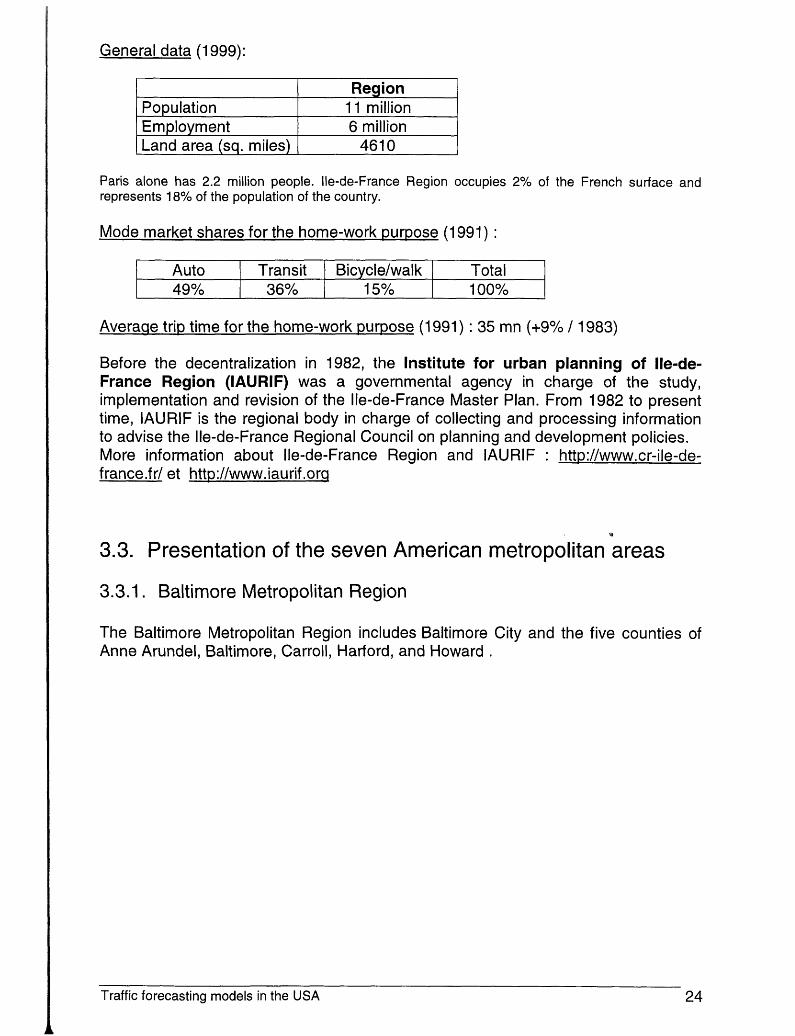
General data (1 999):

Population Region

1 1 million I Emplovment I 6 million I I Land area (sa. miles) I 461 0 I

Paris alone has 2.2 million people. Ile-de-France Region occupies 2% of the French surface and represents 18% of the population of the country.

Mode market shares for the home-work purpose (1 991) :

I Auto I Transit I Bicvcle/walk I Total I I 49% I 36% I '15% I 100% I

Averaqe trip time for the home-work purpose (1 991) : 35 mn (+9% / 1983)

Before the decentralization in 1982, the Institute for urban planning of Ile-de- France Region (IAURIF) was a governmental agency in charge of the study, implementation and revision of the Ile-de-France Master Plan. From 1982 to present time, IAURIF is the regional body in charge of collecting and processing information to advise the Ile-de-France Regional Council on planning and development policies. More information about Ile-de-France Region and IAURIF : http://www.cr-ile-de- france.fr/ et http://www.iaurif .orq

z4

3.3. Presentation of the seven American metropolitan areas

3.3.1. Baltimore Metropolitan Region

The Baltimore Metropolitan Region includes Baltimore City and the five counties of Anne Arundel, Baltimore, Carroll, Harford, and Howard .


- ~ _ _ , . - . . .. . . . ... -

Auto 90%

I I

Transit Bicycle/wal k Total 7% 3% 100%

i

Auto

.- -


Transit Bicycle/wa I k Total

I I

87% 5%

Mode market shares for the home-work purpose (1 990) 8:

8% 100%

Change in transit work trip market share from 1980 to 1990 : - 26%

Averaae trip time for the home-work purpose (1 990) : 20 mn

The Transportation Steering Committee (TSC) is the Metropolitan Planning Organization for the Baltimore Region. It is directly responsible for conducting the con tin ui ng , cooperative and corn pre hensive ("3C" ) transportation planning process for the Baltimore Metropolitan Region.

The Baltimore Metropolitan Council (BMC) provides professional planning staff support to the TSC and is responsible of the traffic model for the region.

Average national mode shares for the home-work Durpose (1 990) :


More information about the TSC and the BMC : http://www. bal tometro.org/

Population Employment Land area (sq. miles)

3.3.2. Washington DC Metropolitan Region

Extended region Region 5,2 million 3,9 million 3,l million 2,6 million

6 800 3 011

The Washington DC Metropolitan Region is comprised of the District of Colombia and eight counties : Alexandria, Arlington, Charles, Fairfax, Frederick, Loundoun, Prince George, Prince William.

Auto

a

Transit Bicycle/walk Total


81 Yo 15% 4% 100%

Mode market shares for the home-work Purpose (1 990) :


Average trip time for the home-work Purpose (1 990) : 30 mn (+9% / 1980)

The Transportation Planning Board (TPB) is the federally designated Metropolitan Planning Organization for the region.


Staff support to the TPB is provided by the Department of Transportation Planning of the Metropolitan Washington Council of Governments (COG).

But recently COG has enlarged the study area . It is comprised of 22 jurisdictions,

suburban Maryland and one county in West Virginia. I spanning the district of Colombia, the greater portions of Northern Virginia and

For more information about COG and TPB : httD://www.mwcog.ora/

3.3.3. New York Metropolitan Region

New York Metropolitan Region covers a part of the tri-state region in New York State and encompasses 10 counties, 190 local municipalities, and a variety of authorities and special districts.

The region is made up of the City of New York (which has itself 5 counties), Nassau, Putnam, Suffolk, Rockland, Westchester. The agency is in the process of incorporating Orange and Dutchess Counties into the planning area.

The extended area corresponds to the traffic model version 2, which is being developed at the moment. 9



I I MTCReaion I I Powlation I 1 1.3 million I I Emdovment I 5.0 million I I Land-areaKa. miles) 1 2345 I


Auto I Transit I Bicvcle/walk I Total


Averaqe trip time for the home-work purpose (1 990) : 31 mn (-8% / 1980)

The New York Metropolitan Transportation Council (NYMTC or the COUNCIL) is the MPO for the New York Metropolitan Region

There are also other MPOs in the tri-state region : one each for Orange and Dutchess Counties (New York), one in northern New Jersey and six in southwestern Connecticut.

For more information about NY MTC : htt p://www. nvm tc. o rq/cqi- bin/welcome2. pI

3.3.4. Boston Metropolitan Region B

The Boston region has 101 cities and towns.


. Hamilton -

Salem Marblehead - - Box- Acton - -

Nahant Lexington Medford --Maiden -~ -- Arlington Everett R~~~~~ Lincoln

Wa,tham Belmont Somervi! Wafer- Cambridge .-

Chelsea

Weston E ... Winthrop

Sherborn Dover - - Milton - - - - - - Westwood Medfield Holliston

NIILford Medway --_

- Marshfield - Franklin

Ll

Region

Rockport

Employment Land area (sq. miles)


1 ,7 million 1422

Auto 76%

Transit Bicycle/wal k Total 14% 10% 100%



Average trip time for the home-work purpose (1 990) : 24 mn (+4% / 1980)

The Boston Metropolitan Planning Organization is one of the 13 Massachusetts regions established to carry out federally funded transportation plans and programs.


I

I

This study was realized in the context of a three-months research between

September and November 1999 in the Institute for Policy Studies of Johns Hopkins

University (Baltimore) as a senior fellow. A one-month business trip in October was

made in order to meet experts and practictioners of traffic modeling in seven cities :

Baltimore, Washington DC, New York, Boston, Chicago, San Francisco, 10s Angeles.


The Central Transportation Planning Staff (CTPS) provides technical and policy- analysis support to Boston Metropolitan Planning Organization and other members of the regions transportation community.

For more information about CTPS : httD://www.ctDs.ora/bostonmDo/

3.3.5. Chicago Metropolitan Region

The region is located in the Northeastearn Illinois and comprised of the city of Chicago, six suburban councils in Cook County, and one council for each of the five collar counties (DuPage, Kane, Lake, McHenry and Will).

.__ ... ..... ........

... :%r:ii wesr C& - .

.........................

DuPo,qe

*- 3

...................

;T"i N

...................................

..................



Population Em dovm e n t

~~ ~

Region 7,5 million 4.0 million

I Land area (sa. miles) I 3842 -1

Auto 80%


Transit B i c yc I e/wa I k Total 15% 5 yo 100%

L I I I I


Averaqe trip time for the home-work Purpose (1 990) : 28 mn (+7% / 1980)

The Chicago Area Transportation Study Policy Committee (CATS) is designated by the state and local officials as the Metropolitan Planning Organization for the greater Chicago region.

For more information about CATS : http://www.catsmpo.com/

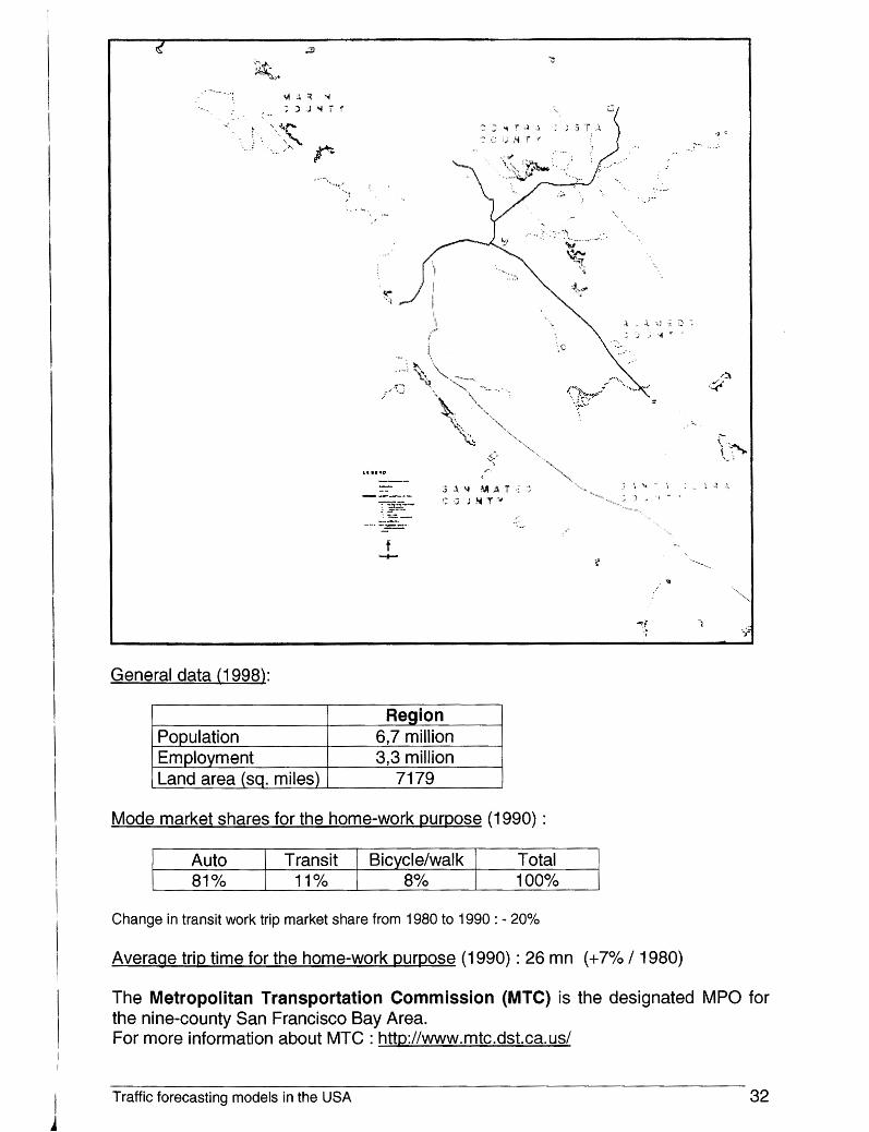
3.3.6. San Francisco Metropolitan Region

This region, called the San Francisco Bay Area, embraces nine counties : Sonoma, Napa, Solano, Marin, Contra Costa, Alameda, San Mateo, Santa Clara, and San Francisco.

B


.'LC . .- -,

Population Employment

.. . .,

~

Region 6,7 million 3,3 million

e

Auto 81 Yo


Transit Bicycle/walk Total 11% 8% 100%

1 Land area (sq. miles) 1 71 79



Averaae trip time for the home-work purpose (1990) : 26 mn (+7% / 1980)

The Metropolitan Transportation Commission (MTC) is the designated MPO for the nine-county San Francisco Bay Area. For more information about MTC : http://www.mtc.dst.ca.us/


3.3.7. Los Angeles Metropolitan Region

Population Land area (sq. miles)

The Region includes six counties (Imperial, Los Angeles, Orange, Riverside, San Bernardino, Ventura) , 184 cities.

Region 16,2 million

38 000


Auto Transit Bicycle/walk Total

Mode market shares for the home-work purDose (1 990) :

92% 5% 3% 100%



Averaqe trip time for the home-work purpose (1 990) : 26 mn (+I 2% / 1980)

The Southern California Association of Governments (SCAG) is a regional planning agency and a Council of Governments comprised of 184 cities in six counties. It has been designated by the federal government as the MPO of the six counties region in Southern California.

More information about SCAG : http://www.scaq.ca.aov/

3.4. IAURIF’s model

In Ile-de-France region, there are several regional models, all different each other. Each actor having a role in the regional planning has its own traffic model : the Regional Service of Public Works in He-de-France (DREIF), the two transit operators Paris Public Transit Authority (RATP) and National Railways Society (SNCF), the Syndicate of Parisians Transportation (STP) and the Ile-de-France Urban Planning Agency (IAURIF). In the 196Os, IAURIF was the leader of the region as concerned forecasting models. But it lost this leadership after the 197Os, especially because of the decentralization and other problems of organization (constitution of a stable technical staff). In 1993, IAURIF had hardly no operational model but a simple demand model adapted from the French software OPERA. It decided to invest in a new model from scratch. The goal at that time was to catch up rapidly the delay without investing in a too sophisticated model.

This is a short overview of the current model, developed fully by IAURIF :

Zoninq . 488 zones + 34 external zones All the zonal data and the networks are stored and updated in a GIs. The GIS bas in particular a very rich coverage describing the land use. All networks and data coverages are cross-referenced to a unique coverage, the land use. The same scale is adopted for data representation.

0

Generation . 10 purposes . No market segmentation Mobility rates per purpose extracted from household surveys. No multiple regression.

Distribution . Standard gravity model . Impedance based on travel car time on a congested network. These times are got after a feedback process.

Modal choice . No logit model, but simply diversion curves. The mode choice has two alternatives for each purpose : car trips and transit trips. The curves are based on the ratio of door-to-door transit travel time to door-to-door highway travel time. The higher the ratio of transit to car travel time is, the lower the probability of choosing transit is.


. The variables taken into account concern only the level of service of each mode, and not the socio-economic features of the traveler or of the zones.

Assianment . For highways, the Wardrop equilibrium method is used. The speed-delay curves are those of the software DAVIS, commonly used in France. . For transit, all-or-nothing assignment.

Software . MINUTP, ARCINFO and SAS. IAURIF developed an interface between these two software in 1995. This interface was designed since the beginning of the project and is quite operational today. The GIS allows to prepare easily the data (for example, the networks in both software are the same). As a post-processor, it allows to generate results very quickly and to produce automatically some standard maps. Thanks to this interface, IAURIF has gained a lot in productivity and in maintenance. For more information about this interface, see httD://www. es ri .com/li bran//userconf/euro~roc96/PAPE RS/PN4 1 /PN4 1 F.HTM

In 1998, because of the limits of MINUTP in memory, IAURIF purchased another software, DAVISUM, developed by PTV Systems in Germany. Now the model under MINUTP is in the process to be moved in DAVISUM.

IAURIF has the same concerns than its American counterparts. One of the-major goals has become to forecast changes in travel demand induced by alternatives policies to highways capacity increasing. Emphasis has shifted from long-run planning of highways networks to short-run planning and to management of multimodal transportation system. These shifts have placed considerable strains on the current conventional forecasting model which was originally developed to address problems of highway network design.

3.5. The seven American cases’ models

This part will provide technical descriptions and some general impressions about seven models. No doubt the technical descriptions, which level of details vary following the case, are incomplete and maybe outdated. They sum up only the available documents and the minutes of the interviews. As far as concerned the comments, they might tackle with touchy fields (organization for example).’ They reflect only the opinion of the author.

3.5.1 . Baltimore’s model

Since the passage of ISTEA, the Baltimore Metropolitan Council (BMC)’s regional model has undergone a significant number of changes. It benefits from the help of a consultants firm.


Zoning : ' 804 zones (of which 207 just for Baltimore City). BMC has constantly been

expanding the area covered by its model. Recently, the study area was expanded to three counties belonging to the Washington DC region. The interaction between Baltimore and Washington continues to grow (30% of the workers of Howard and Arundel counties commute to the Washington DC region). There is a good cooperation between the MPOs of Baltimore and Washington, especially to exchange data. The land use is classified in 4 types : city center, urban, suburban, rural.

Generation : Market segmentation function of the number of people per household and the number of vehicles per household (totally 13 classes). BMC plans to add another crossing criteria : household income.

' There is a mobility rate for each purpose and each class of population. . Six purposes The generation model is made by a regression analysis with the software SPSS. Six variables were identified as determining the trip generation : licensed drivers per household, persons per household, employed persons per household, driving- age per household, household income, car ownership level. . Specific generator for Baltimore-Washington International airport

Distribution : Standard gravity model . The impedance is the travel time by car on a free flow network. But BMC is aware that using only these times ignores the potential influence of high capacity public transportation. The validation is realized just after each step thanks to the information of the 1993 travel survey. Reference trip tables of 6*6 dimensions (county to county origin- destination) are calculated from the sutvey and compared to the model results.

Mode choice : It seems that the mode choice model is very old (1 959). The transit trips are just taken out of the all-motorized modes matrix by look-up tables. These tables split home-based work person trips into vehicle driver, vehicle passenger and transit passenger. They are based on a lot of variables : transit and highway travel times and cost, income, parking costs, and both residential and employment density. All these variables are monetarized to 1959 dollars because the original model was calibrated on these costs. However, there is a sophisticated model (a logit) to simulate the car occupancy, that means to split into SOV (Single Occupancy Vehicles) and HOV (High Occupancy Vehicles) users. The same mode choice model has been used for about 30 years. BMC is developing a new one with the help of consultants. The project began in October 1998 and is scheduled to be completed in 2000. The goal is to be able to model n on -mot o r ized modes, al t e rn at ive test i n g , congestion pricing , travel demand management (TDM). After a thorough research, BMC decided to conduct a stated preference survey this year (1999) which can collect travel mode choice

Traffic forecasting models in the USA :36

preferences from both transportation users and non-users, so as to provide more reliable data to estimate the value of time.

Assignment . For the highways, a four increment process (40% + 3*20%) with capacity restraint is used. BMC is thinking about a new function of assignment :

T/To = 1 + 0.2 (V/C)’Ofor freeways and T/To = 1 + 0.05 (V/C)’O for other roads

. The model can run for five time-periods in the day.

Software :

BMC has encountered problems with this software because of its limits in memory. So it has purchased an other one, TP+ and VIPER for the graphical interface. Now BMC is moving its current model under MINUTP to TP+. It plans to introduce a GIS tool in the modeling chain.

MINUTP and SPSS

Comments BMC has still a very oriented-highways culture. It’s very obvious when you find out the very old mode choice model : it’s the only one among all MPOs which doesn’t use the best-of-the-practice yet (the logit model). But a new modal choice model is expected for next year. The highways network doesn’t incorporate the turning movements. So BMCk model can only be used for studies at a regional scale. There is also a lack in the modeling process that could some day bringgaboutjwidical problems : the model can’t simulate the interaction between land use ,and transportation. BMC is very interested to develop an interface between their model and a GIs. BMC and COG work very closely

3.5.2. Washington DC’s model

In response to the requirements of ISTEA, the Council Of Governments -“(COG) formulated in 1993 a multi-year models development, re-examined it in 1995 by a peer review panel and further restructured it in 1998 by a Travel Forecasting Subcommittee. So there is a real effort to update and maintain the regional traffic model, and especially to extend it to the expanded region. Two versions are being developed. The version 1 is the current model. The version 2, being devejoped, differs from the version 1 in that : - -

it takes more purposes and more market segments into account. it will be able to deal directly with some periods of the day (morning and evening peak periods, off-peak period). That is necessary for the input of the emission model

Traffic forecasting models in the USA -. 37

- It has the same zoning for the four steps, whereas the version 1 has two different zonings, one for the demand and the other for the assignment.

In 1999, the version 1 should be completed as well as some components of the version 2.

The documentation provided by COG is very well detailed and clear. This is an overview of the version 2 model :

Zoning : 2145 zones, plus 47 external zones. The version 1 of the model has only 300 zones for the generation and 1500 for the assignment.

’ COG is faced with the problem of definition of the study area. For the version 2, it expands the region cordon. But it doesn’t go until including Baltimore city.

Networks COG has been using ARCANFO tools as a pre-processing. But there is no unified database yet : the networks on the GIS and on MINUTP are different. So the editing of links (adding new links, splitting existing links) is conducted in both MINUP and ARC/INFO simultaneously. It’s a heavy work. GIS is also used for some analysis. For example, a walk access to transit file is generated thanks to an ARC/INFO procedure. After the transit lines were brought into ARC/INFO database, a simple buffering routine around each transit stop node was used to identify the short-walk and long-walk areas in each zone.

Generation . Market segmentation function of household income, car ownership level and household size (totally, 64 cross-classes). The COG’S model has two demographic programs which simulate household income and vehicle ownership. Four trip purposes and in addition two for truck trips (separated into medium and heavy truck trips). Different mobility rates characteristic of different parts of the region.

Distribution Standard gravity model The impedance is a composite time function that represents a blending of transit and highway service levels. In the version 1, the distribution model is based only on highway travel times.

where : CTi : composite time for segment i HT : real highway time TT : real transit time Pi : regional transit share of segment i

The highway and transit times used in the formulation vary by purpose.

Traffic forecasting models in the USA .38

Mode Choice The model consists of four sequential logit models, one for each purpose. Five modes are dealt : transit, drive alone, group ride (2 occupants), group ride (3 occupants), group ride ( more than 3 occupants). . It’s a staged multinomial logit model. The upper stage of the model splits trips into drive alone, carpool and transit trips. The lower stage of the model splits carpool trips by occupancy level : 2, 3, 4 or more persons per vehicle. The model application is market segmented by car ownership level (0,1,2 or more). This is not a nested choice model in that the carpool occupancy level utilities don’t affect the overall carpool utility in the upper stage multinomial logit model. The model was estimated using COG’S 1994 household travel survey. . Factors considered in the model include accessibility of mass transit, car ownership, proximity to carpool lanes, costs, and time. The cost variables represent “out of pocket” costs, including mass transit fares, the price of gasoline, parking, and a mileage rate for driving. Time variables include time spent waiting for transit, time transferring between routes, or time spent to drive and park the car and reach the final destination. The mode choice factors are introduced in an equation that estimates the probability of each traveler selecting each mode, given the characteristics of both the mode and the traveler. Among the most important factors in mode choice are average parking costs and the time it takes to walk to the final destination from parking spaces or transit stops. Average parking costs for each zone are function of the zonal employment density. Thus, heavily used downtown zones have the highest parking costs, and zones with fewer workers per square mile have lower parking costs. Zones with fewer than 10000 work trip attractions per square mile are assumed to have no parking cost. . For mass transit riders, further assumptions are made about their use of bus or rail, and, for rail users, about the stations chosen and the wayBeach traveler reaches his or her station. For example, only persons within four-tenths of a mile of a station are assumed to walk to the station. The model assumes that the rest of the transit users either drive, or are dropped off at their station. For logit model estimation, over 80 candidate model forms were estimated using ALOGIT. It’s a heuristic, trial-and-error process, well known by the practitioners. A land use variable is taken into account into the transit and highway utility equations :

land use mix index = (hhpopd*nempd) / (hhpopd + nempd) where : hhpopd : household population density

nempd : normalized employment density

Software : MINUTP, ARCINFO and SAS.

COG has problems with this software because of its limits in memory. So it plans to buy an other one, TP+.

Miscellaneous The cost of maintaining and applying the models constitutes a little more than‘50 percent of the region’s transportation planning budget, or about $2.6 million per year. Modeling to test the air quality conformity of the proposed Transportation

Traffic forecasting models in the USA I 39

Thanks to

all the staffs members of the Institute for Policy Stud&,iespecially

Sandra Newman, Director

Marscha Schachtel, senior research fellow

Joseph Harkness, senior statistician

Laura Vernon- Russell, assistant

Thanks to

all the persons who accepted to receive me for an interview (see appendix)

Thanks to

the other international fellows : Ayla, Hiroko, Sylke, Eric, Jason, Pierre. pl


Improvement Program (TIP) required the expenditure of more than $100000 for staff and other resources over a recent two-month period.

Comments It seems that COG3 model is one of the clearest models, not too sophisticated and not too simple. The advantage is that it becomes easy to maintain it. An important work consists in unifying the networks database of GIS and MINUTP. Another lack of the model is the absence of interaction with land use model.

3.5.3. New York’s model

Since 1992, NYMTC has been developing a transportation demand modeling system to address CAAA and ISTEA requirements as a long range transportation forecasting tool. It includes two steps : The Interim Analysis Method (IAM) and the Best Practice Model (BPM).

The IAM was developed to address transportation forecasting needs in the short term, addressing CAAA and ISTEA requirements prior to the availability of the BPM. The IAM is regional in its coverage, network-based, multi-modal, sensitive to highway travel times and congestion, and is based on a single set of adopted future socioeconomic growth forecasts common to all transportation studies in region notably both in highway and transit. The IAM uses a set of synthesized vehicle trip tables, a set of peak and daily regional highway networks, assignment procedures, and post processing tools.

The BPM is being developed as the second phase to comprise the augmented databases and advanced-methods in the NYMTC Transportation Models and Data I nit iat ive project . With more than 8 million dollars, the main categories of the work are :

‘J

- - Develop Land use model, - Develop database management system, - -

Develop demographic and economic forecasting,

Finalize networks and analyze zone system, Collect & process travel and transportation data (household travel survey, external auto cordon survey, supplemental speed data collection, supplemental highway count data collection, assemble key available transportation data sets), Develop calibration and validation files, Estimate and implement model system, Test model applications (both base and future year forecasts), Plan for future model extension.

- - - -

Developed by a consultants firm, the new model should be released in the end of 2000. The specifications of the model are very ambitious because they call for the st at e-of -t h e-a rt .

Traffic forecasting models in the USA / 40

The following figure represents a conceptual structure of the NYMTC Best Practice Models set.

? I

,-..-..-..-..-..-..-..-. '-.'-..-.'-"-".-... I i

HIGHWAY NETWORK

TRANSIT NETWORK

VEHICLE OWNERSHIP

MARKET SEGMENTATION

I ACCESSANALYSIS

C-- I I

I I

I

I HIGHWAYASSIGNMENT I

b

I 1 LAND USE i

I PRIMARY DESTINATION -------J

FREQUENCY TIME-PERIOD for work/school

t I

[ TRANSIT ASSIGNMENT I

TRANSIT REPORTING

HIGHWAY REPORTING Legend

Trips and Impedances ..." .......... .. ....

LogSums Feedback b o p s

Conceptual Structure of the NYMTC Model Set

-.--.-.--..

Traffic forecasting models in the USA - 41

This is an overview of the new expected model :

m: 3500 zones. NYMTC is faced with the boundaries of its study area. The last national census (1990) showed that trips to Manhattan from the suburbs have remained relatively stable between 1980 and 1990 while trips from New Jersey increased dramatically from 172 000 to 218 000 (+27%) . Moreover a lot of old data use the Tri-State region as a geographical area.

Activitv based model Market segmentation based on socio-economic characteristics (home, household size, car ownership, number of workers). Five purposes Journey based model (not trips). NYMTC defines the term journey as a movement between two key or principal locations that establishes anchor points in the travel patterns for each household member. A tour is considered to be a movement from home to one or more locations and then returning home. A tour is composed of one or more journeys. For travel involving “committed activities”, the principal locations are for the residence, the workplace, and the school location. For other travel, the principal non-home location is the point on a journey that is the most distant. A set of models, called Travel Pattern Model, will explain how, when and where journeys are made. There are several tiers to the Travel Pattern model set. First, it will be to determine the type of journeys that will be generated. These could be for committed activities, which are essentially work or school trips, or for non- committed activities, which are comprised of trips for all other activities, such as shopping, personal business, etc. Travel patterns for the committed activities will be estimated considering: - A joint activity type/location decision for the geographic distribution of

committed travel, with variations by activity type. - Travel frequency will be estimated for the share of student or workers who

make journeys to school or work on an average weekday, and the number of journeys made.

- Time of the day will be addressed for the work and school trips over five time periods of the day (AM and PM peak, midday, evening and night).

- Travel patterns for the non-committed activities will be determined as follows : .

u

The travel frequency model will be used to estimate the share of persons who will make specific number of non- workhon school tour.‘This component applies to individuals rather than households. Primary destination model then predicts the primary destination for each tour. The primary destination will be the location most distant from home or where the individual spent the longest time. This will be a multinomial logit model.

There is also an vehicle ownership model. It will determine the number of vehicles available to households for use in travel. The model will take into account the influence of household income, vehicle maintenance, parking availability,

Traffic forecasting models in the USA -42

accessibility, and household characteristics to estimate vehicle ownership of a household.

Walk trips

Distribution It's not a classical gravity model but a logit model :

The probability that a trip from zone i will go to zone j is : exp(a * IMPij + b * LNDj)

pij = ---------------------------------.--.-------- SUM, { exp(a * IMPi, + b * LND,) }

Bicycle trips

Where : IMPij : measure of travel impedance from i to j LNDj : a set of descriptors of the land use in zone j a, b : vectors of the coefficients

Shared ride Drive alone trips trips

Mode choice The method proposed by the consultants firm is considered as the best-of-the- practice : the nested logit model. The suggested structure of the mode choice model is shown below :

Local & express Rail trips Commuter rail bus trips trips

A

I Person trips I

'I Walk to station Feeder bus to Park & ride to Kiss & ride to

station trips station trips trips station trips

I

Same sub-mode

selection and station

f

Two persons per car trips

Non-motorized trips

Three persons per car trips

I Transit trips I

Free Toll Station A Station B Station C -

Station D A

It estimates the four primary modes : transit, highway, taxi and non-motorized, Under the transit mode, the model will distinguish between rail trips, commuter rail trips and bus trips, both local and express. The rail mode and the commuter rail mode will


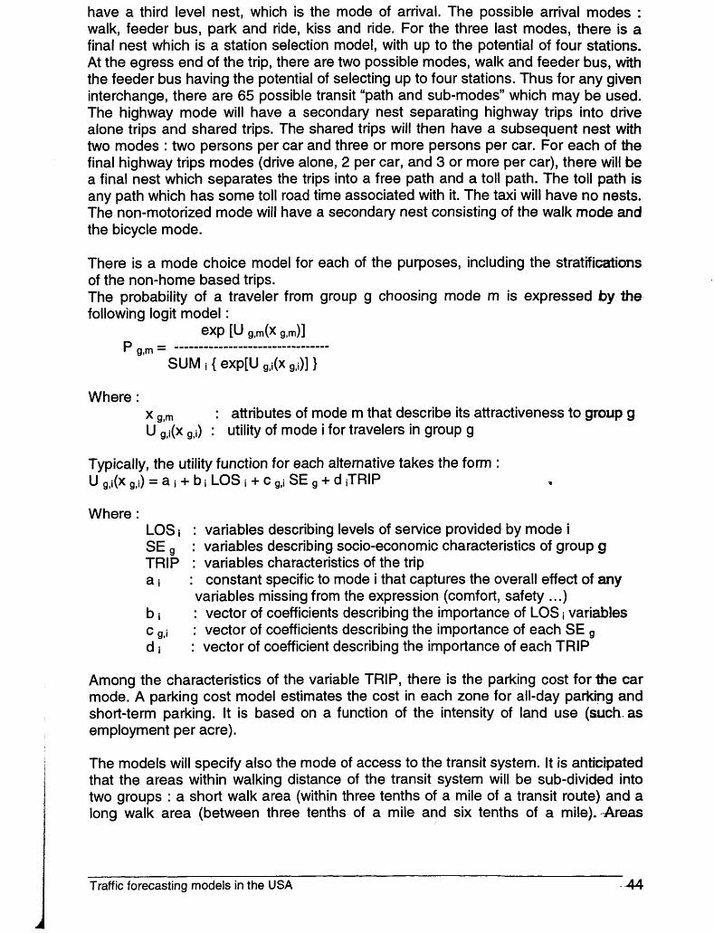
have a third level nest, which is the mode of arrival. The possible arrival modes : walk, feeder bus, park and ride, kiss and ride. For the three last modes, there is a final nest which is a station selection model, with up to the potential of four stations. At the egress end of the trip, there are two possible modes, walk and feeder bus, with the feeder bus having the potential of selecting up to four stations. Thus for any given interchange, there are 65 possible transit “path and sub-modes” which may be used. The highway mode will have a secondary nest separating highway trips into drive alone trips and shared trips. The shared trips will then have a subsequent nest with two modes : two persons per car and three or more persons per car. For each of the final highway trips modes (drive alone, 2 per car, and 3 or more per car), there will be a final nest which separates the trips into a free path and a toll path. The toll path is any path which has some toll road time associated with it. The taxi will have no nests. The non-motorized mode will have a secondary nest consisting of the walk mode and the bicycle mode.

There is a mode choice model for each of the purposes, including the stratifications of the non-home based trips. The probability of a traveler from group g choosing mode m is expressed by the following logit model :

~ X P [U g,m(X s ,d l p g,m = -----_------------_-______I_____

SUM i { exp[U g,i(X g,i)l I Where :

X g m : attributes of mode m that describe its attractiveness to group g U g,i(X g,i) : utility of mode i for travelers in group g

Typically, the utility function for each alternative takes the form : U g,i(X g,i) = a i + b i LOS i + c g,i SE g + d iTRlP B

Where : LOS i : variables describing levels of service provided by mode i SE : variables describing socio-economic characteristics of group g TRIP : variables characteristics of the trip a i : constant specific to mode i that captures the overall effect of any

variables missing from the expression (comfort, safety . . .) b i : vector of coefficients describing the importance of LOS i variables c g,i : vector of coefficients describing the importance of each SE d i : vector of coefficient describing the importance of each TRIP

Among the characteristics of the variable TRIP, there is the parking cost forthe car mode. A parking cost model estimates the cost in each zone for all-day parking and short-term parking. It is based on a function of the intensity of land use (such-as employment per acre).

The models will specify also the mode of access to the transit system. It is anticipated that the areas within walking distance of the transit system will be sub-divided into two groups : a short walk area (within three tenths of a mile of a transit route) and a long walk area (between three tenths of a mile and six tenths of a mile) ... Areas

Traffic forecasting models in the USA -44

beyond the long walk distance will be considered as having only access to9ransit. Highway access though will be available for the short and long walk areas.

Feedback Congestion effects are fed back to trip generation, trip distribution and mode choice.

Land use model NYMTC Land Use Model (LUM) will be adapted from the structure of the METROSIM model which is the proprietary Land Use Model developed by a consultants firm. This land use model forecasts the number and location of households and non-residential activities by type, together with land use and land use changes by zone. It includes economic models that take into account the effects of accessibility on land prices and rents and the subsequent effect on local decisions. This firm will develop for NYMTC an interface between the LUM and the traffic model. The interface will allow for feedback passes. Technically, many iterations are necessary to reach an equilibrium. With 3500 zones, the LUM would potentially consist of 1 0500 simultaneous equations and variables which are determined simultaneously. The LUM will be capable of being operated as “constrained”, by external forecasts. A single model of commuting patterns to be used by both the land use models and transportation models will be developed using the 1990 CTPP and the 1996/1997 Household Interview Survey (HIS). The land use models will use the commuting patterns to estimate zone-level housing demand and non-basic employment. The travel demand models will use full set of land use model outputs to start the estimation of travel patterns. NYMTC evokes also the project to develop a full GIs-interfaced LUM.

Software NYMTC has used TRANPLAN for highway analysis, TransCAD for transit analysis, and TRIPS for synthesized trip table. as part of IAM. In BPM, NYMTC will use TransCAD with customized ultility programs and user friendly interface as the software package for model application, file management and data analysis. NYMTC uses ALOGIT for choice models’ parameters estimation.

Miscellaneous NYMTC is about to begin updating its regional population and employment forecasts to the year 2025. The current forecasts, which were developed in 1994/1995, extend to the year 2020. The 2025 forecasts will be developed, under the guidance of the NYMTC’ staff by a consultants firm.

Comments The specifications of the model to be developed are very ambitious because-they reach the state-of-the-art (especially the activity based model). NYMTC has chosen to develop from scratch. It’s sure that if you try to develop existing code (what is commonly called “reengineering software”) you can only achieved small improvements. In New York City, there is a very high share of taxis rides, higher than anjmhere in the USA. It’s important to take this mode into account in the new model. All the players in the transportation planning in New York expect a lot of the new model. But it seems that the project will be delayed.

Traffic forecasting models in the USA ,45

New York region is a huge metropolitan region, with a lot of heterogeneous aspects and a lot of actors in transportation planning. One of the problems of NYMTC is to take into account all the needs of these stakeholders. NYMTC has also to take into account the outside of its boundaries, especially the region of New Jersey and to be compliant with the other MPOs of the Tri-State Region.

3.5.4. Boston’s model

Central Transportation Planning Studies (CTPS) maintains the regional model that is used by the Boston MPO and other transportation agencies. It’s now involved in a process of enhancement, so there’s no documentation describing CTPS’ model yet. The new model is designed as a highly sophisticated and data intensive planning tool and should be operational next year. The overview of the model below is obtained through some traffic studies reports dating from the early 1980s. So the model, called CARSIM, is old but some procedures will be still used. Furthermore, CARSIM includes an emission model

Zoning : 775 zones + 102 external zones . CTPS is faced with the definition of its study area. It is clear that Boston’s commuters are not confined within the boundary of the Boston Metropolitan Planning Organization region. In 1990, of the 500000 total commuters to Boston, more than 50000 people commuted from outside of the Boston MPO region, and of those, more than 10000 commuted from out of state. It’s why CTPS has defined an extended region, roughly corresponding to a seventy-mile radius around Boston. Called the MPO Commuter Source Area, it includes 388 cities and towns in five New England states. It’s is a very large region, hbme to nearly seven and a half million people (more than twice the population of the MPO region).

Gene rat ion 4 purposes . Logan international airport is a special generator. A specific model simulates the demand.

Distribution . Gravity model As impedance, a composite highway and transit travel time defined as follows is used :

CH = CF*P + (1 - CF)*OP T = IVT + 2.5*0VT

Where : CH : composite highway travel time P : peak highway travel time OP : off-peak highway travel time CF : congestion factor T : morning peak period weighted transit travel time IVT : total in-vehicle and car access travel time


1

OVT : total out-of-vehicle walk, wait and penalty time Then the resultant highway and transit time are combined, using - a parallel conductance formula, into the composite impedance I which is used in the gravity model for each purpose :

1

(l/CH) + (In 1928)

Mode choice The mode choice model is simply based on curves for each purpose.‘These curves are function of the generalized costs difference between car and transit, the length of trip and the level of car ownership at the production zone (for home-based trips) or percent transit of home-based trips at the attraction zone (for non-home-based trips). The generalized costs include out-of-pocket costs (such as transit fare, parking fees and car operating costs) and trips travel times (converted to monetary value), which are calculated based on the minimum time paths for the interchange. during tbe morning peak period.

CT = 4.17 [(IVT + AAT) + 2.5*0vTJ + (AAT/GO) (20) (3.47) + FARE CA = 4.17 [IVH + 2.5*OVH] + [(3.47) (DIST) + 0.5 (PARK)] (I/AO)

Where : CT : transit generalized cost CA : car generalized cost IVT : in-vehicle transit time (mn) IVH : in-vehicle highway time (mn)

AAT : car access time to transit (mn) OVT : out-of-vehicle walk, wait, and car access penalty time (mn) which is

OVH : out-of-vehicle highway time, or terminal time (mn) DIST : highway trip distance (miles) PARK : average zonal parking cost FARE : transit fare

fixed at a value of 10 mn

A0 : average attraction zone car occupancy (personskar) 2.5 : factor to convert out-of-vehicle time to equivalent in-vehicle time

4.17 : constant to convert time to cost 3.47 : average car operating cost 20 60 : mn/h

: average car access speed of 20 mph

These last five numerical values make reference to the 1963 base year:‘This model was used in 1987 to forecast the traffic expected for the Central Artery Project (‘The Big Dig”), biggest highway project in the USA today.

Calibration The calibration adjustments are made after each step. It’s better to cabate at the end of each step rather than once in the end, because there is a cumulative effect of errors or inaccuracy.

Assicln ment The stochastic method is used.


Soft ware TRANPLAN is used for assignment only. For the new model, EMME 2 has been purchased. . CTPS plans to develop its GIs, above all its graphics capacities (design and production of maps). It supports the GIS used by Massachussets DOT to manage and monitor the state highway network

Comments CTPS’new model is in the stage of calibration. The innovations are the followmg : - The steps of distribution and mode choice are grouped in one step only. - A specific kind of trips will be incorporated in the model : the itinerant trips. - The taxi model will be updated. - The new capabilities of assignment in EMME 2 will be used A documentation about the model development and the calibration processes wili be released. Parrallely, CTPS is developing a GIS as a support for land use analysis and transportation planning. But there is no project to interface the traffic model with the GIs.

3.5.5. Chicago’s model

The Chicago Area Transportation Studies (CATS)’ case is very interesting because it’s the only MPO in the our seven study cases which claims to use the land use model DRAM/EMPAL (Disaggregate Residential Allocation Model/Employment Allocation) lo to elaborate its regional transportation plan. CATS worked in close cooperation with another agency, the Northeastearn Illinois Planning Commission (NIPC). NIPC and CATS worked cooperatively on an extensive asalysis of the relationship between transportation and land use as an initial step in the development of the forecasts and regional transportation plan. They called for a professor, Or David Boyce from the University of Illinois (see [22]), to develop an interface between the traffic model and DRAM/EMPAL. The process works on five-year increments starting with the base year 1995 and stepping out to the year 2020. At each five-year increment, the forecasted total of households and employment are allocated spatially taking into account the transportation infrastructure assumed to be in place at that time. Some experts criticize DRAM/EMPAL in that at first it doesn’t incorporate in its parameters the pricing factor and secondly it is very difficult to calibrate.

Of course, the CATS’ model isn’t the only one in the region. In particular, there istbe METRA’S model which is very “competitive”. Because they don’t produce always the same results for the same project, attempts were made to reconcile the two.models in the assumptions, calibration . . .

The technical documentation provided by CATS is very clear. Each step is decribed in details. The main concern of this document is to try to show that the trafic model can satisfy the needs of the air quality analysis required by the federal legislation.

lo Actually, DRAM/EMPAL is used currently in about twenty MPOs in the USA.

Traffic forecasting models in the USA - 48

A

The CATS model is a classical four-steps one, with considerable modifications since 1994 to enhance the distribution and mode choice procedures.

Zoninq . 1640 zones + 30 external zones

Gene rat ion . Market segmentation based on four variables : number of adults, number of workers, vehicles avalaible for use, presence or absence of children in the household. Totally, there 1 12 different household types. Four purposes. . There is a vehicle ownership model (a logit model). . The trip generation model estimates total trips including both motorized tripsand non-motorized trips. The method uses regression equations. . There is a truck trip generation, based on four weight and size classes.

Distribution . Opportunity model (not a gravity model) originally formulated in 1960. . The impedance is a generalized cost mixing transit and highway costs. The Combined Model allows to calculate changing travel impedances in response to changes in the transportation networks and the location of households and jobs.

Mode choice 9 Disaggregate mode choice model . A file of simulated trips records is generated by a random Monte Carlo sampling

process. The following data are used to generate this file : - matrices giving the zone-to-zone travel times and costs for transit and highway - frequency distributions of household income for the origin zones - frequency distribution by zone of the distance from a householddto the nearest

rail transit or commuter rail station, bus stop or feeder bus service - walking distance versus parking cost model for the Chicago Central Business

District (CBD), and parking access data for the remainder of the region. - the 1990 household survey (sample of more than 19000 households) . There are different values of time, depending on the trip purpose, the components of route time (in-vehicle time, headway time, transfer time, walk time, . . .) and h e destination. All cost values used in the model are in 1970 dollars.

9 Then a conventional logit model is used. The mathematical expression is exactly the same than New York's one.

Assianment . Eight time periods of assignment addressed to air quality analysis. . CATS had to face a classical problem encountered at this step : the over- assignment problem. So the classical volume-delay functions have been revised. For example, for metered freeway entrance ramps, the original BPR function is revised so that travel times greatly increase when the link volume exceeds the maximum metered flow rate. This effectively restricts the ramp's volume to the metered flow rate. The adjusted function is :

Tiink = To* (I +O, I 5* (VN0)'O)

Traffic forecasting models in the USA ;49

LE OF CONTENTS

1 . INTRODUCT I ON .......................oo....o.o....o~ ..oo..o..~~.....o~o.o~ 8

2 . 2 . The classical f our-steps model ............................ 11

2 .3 . Improvements of the four-steps model .................. 12

2 . 3 . 4 . As s ignmen t ............................................ .....-.-..- . .-.. ......- . 14

2.4. Tracks of research 15

2 . 4 . 1 . Integration of land-use and traffic models ..-.--. 15 B

2 . 4 . 2 . The activity-based model ...--..........-..- ..-- ...-- ---.... 17

2 . 4 . 3 . Stochastic microsimulation

2 . 4 . 4 . Time departure and route choices ... .. o.... 19

2 . 4 . 5 . Geographical Information System platform --.- 19

2 . 4 . 6 . Interface to air quality model ..........-.-..-. ..-.-- 20

2.5. The future generation of model : TRANSIMS ..- 2 0

3 . STATE-OF-THE-PRACTISE .- 2 3

3.2. Presentation of Ile-de-France Region 23

3.3. Presentation of the seven American metropolitan areas ............................................................... .................. .......o~.o...o.~.~..o.W.o.oo .. 24


Software . EMME/2 and DRAM/EMPAL. The unified package is called the “Combined Model”. . CATS has also another model (PLANPAC) running on a mainframe platform.

Comments The documentation is very detailed for the highways part. There is a lack of information about how transit is dealt, especially for the assignment step. As we were told, the Combined Model doesn’t actually work perfectly. However, the advantage is that while elaborating the regional transpotfation plan, not only different networks were tested but also different assumptions of population and employment growth were used to build scenarios. That means that different demand mafn’ces were used. This represents a major improvement in methodology. Above all, CATS can’t be reproached for not having taken into account the interaction between land use and transportation system. The CATS’S model has undergone steadily updates since the beginning, trying to follow as far as possible the state-of-the-art. It’s important when there are many models running in a region that they can produce roughly the same results for the same tested project. Otherwise it’s all the modeling field that is decredibilized in the view of decision-makers.

3.5.6. San Francisco’s model

The new travel demand model system is BAYCAST, or more specifically BAYCAST- 90 for the 1990 survey-based models. Metropolitan Transportation Council (MTC) has also two old models : - MTCFCAST : MTC Travel Demand Model Forecasting System. It was originally

developed in the 1970s as a state-of-the-art disaggregate travel demand model system, with the contribution of Pr Ben-Akiva. MTC staff redeveloped MTCFCAST in the 1980s using updated networks and data from the 1981 MTC household travel survey. SRFCAST : Short-Range Travel Demand Model Forecasting System. It’s a fully disaggregate model system, SRFCAST, or short-range forecasting system. The SRFCAST is a “sample enumeration” model system applied at the fully disaggregate level to either households and persons from household travel surveys, or to synthetic persons and households.

-

BAYCAST is designed as an advanced state-of-the-practice trip-based travel forecasting system.

The BAYCAST modeling system includes the standard four steps of trip generation, as well as three extra main models: workers in household, car ownership choice, and time-of-day choice models.

The documentation about the model is no doubt the most detailed one in the USA.


Zoning . 1099 regional travel analysis zones internal to the nine-county Bay Area, and 21 external zones. . MTC uses a system of 34 superdistricts for use in calibration (adjustment) and for reporting of standard results. . Previous MTC model systems operated at a 290, 440, 550, 651 and 700 regional zon e-levels .

Hiahwav Network . 31 300 one-way links. . Separate codes are used for mixed flow lanes, HOV 2+, HOV 3+, and restricted access to large trucks. . County geographic location is a variable used in the file for reporting and pbttmg purposes.

Transit Network . 700 transit lines for 25 transit operators. . Morning peak period bus speeds and car access-to-transit speeds are based on congested highway travel times. . Special MTC programs are needed to add station-to-station rail fares to the bus fare matrix. . Networks are created for the morning peak period and off -peak period. Two sets of morning transit paths (walk access only / walk and car access available) and one set of midday transit paths are used in the demand model process.

Travel Survev Database In 1990, MTC conducted a major household travel survey of more than 9300 households for their single weekday travel patterns, and an additional 1500 households for their multiple weekday (3 or 5 consecutive weekday) travel patterns. It is a traditional trip-based travel survey collecting data on trips as opposed to in-home and out-of-home activities. In contrast, the 1996 MTC household survey is a time-use survey, collecting detailed data on in-home activities as well as out-of-home activities (as well as traditional information on trip characteristics.) Another survey will be launched after the national 2000 census.

.

Generation Market segmentation by the number of workers in the household, by cars available in the household, and by household income quartile only for the borne- work purpose. 6 main purposes . Home-based school trips are further broken down into-three other sub-purposes. Trips include non-motorized trips (bicycle, walk) as well as motorized modes (car, transit). With the exception of the home-based school trip generation model, all of the trip generation models are multiple regression in form. The home-based shop trip generation model, in particular, is a hybrid of a market segmentation model (stratified by workers in household level) and a multiple regression model.’ The independent variable in these multiple regression trip generation models are


either mobility rates (e.g., work trips per employed person) or trips (e.g., total home-based social/recreation attractions, total non-home-based productions). MTC is thinking about a future model based on activities.

Distribution 8 Standard gravity model. In the previous model, the home-based work distribution

model was a logit model but it has been given up. m Travel time as used in the BAYCAST distribution model is either morning peak

period door-to-door drive alone travel time, or a blend of morning peak period and off-peak period door-to-door drive alone travel time. In the case of home-based work and home-based school trips, only morning peak period travel times are used. For home-based shop, home-based sociaVrecreation and non-home-based trips, a "blended" travel time based on 32.4% peak and 67.6% off-peak travel time is used.

m Socio-economic adjustment factors (k-factors) are used in calibrating and validating the trip distribution model.

Modal choice The modal choice model is a nested logit choice model with seven basic modal alternatives : drive alone, shared ride 2-occupant, shared ride 3 or more occupant, walk-access-to-transit, car-access-to-transit, bicycle and walk. At the upper level of the nest, work trips are split into motorized, walk and bicycle trips. The middle level nest splits motorized work trips into : drive alone, shared ride 2, shared ride 3 or more and transit. The lower nest splits transit into walk-access or car-access transit trips. Nested logit choice model is applied to each purpose, except for the home-based grade school purpose (multinomial logit). Variables include mean household income, mean household size, the share of households residing in multi-family dwelling units, the share of persons age 62-or-older, and gross population density. Data on mean household income, mean household size and gross population density is available from Association of Bay Area Governments (ABAG) forecasts. This association is a regional agency rather specialized in development and regional land use issues. Future year data on share of multi-family units and share of persons age 62-or-more are derived by MTC staff from 1990 decennial Census data and ABAG county-level age forecasts. An important feature of most BAYCAST mode choice models is that both morning peak period and off-peak period travel times and trip costs are used in the model application. In previous versions of MTC model systems, home-based work trips were only sensitive to peak period travel times and costs whereas non-work trips were only sensitive to off-peak times and costs. This improvement in the model system means that mode choice for these purposes is sensitive to changes in both the peak and off-peak period, as opposed to just one or the other. All mode choice models incorporate non-motorized alternatives: bicycle and walk- only. Travel times for bicycle and walk are based on a "non-motorized network" based on the standard regional highway network, excluding freeway facilities where bicycles and pedestrians are not allowed and including freeway facilities where bicycles and pedestrians are allowed. Uniform speeds of 3 miles per hour for pedestrians and 12 miles per hour for bicyclists are used to convert nom motorized distance into travel time.

~- ~


. Other example : the nested non-home-based (NHB) mode choice model includes five alternatives (driver, passenger, transit, bicycle, walk) and one nest (motorized trips). The upper nest for the NHB mode choice model splits trips into motorized, bicycle and walk modes. The lower nest splits motorized trips into vehicle driver, vehicle passenger and transit modes.

Departure Time Choice Mode The departure time choice model included in the BAYCAST model system is a simple, binomial logit choice model with two alternatives:

- leave from home-to-work between 6:30 and 8:30 AM (peak); - leave from home-to-work before 6:30 or after 8:30 AM (off-peak).

The model is applied only to home-to-work car person trips. The departure time choice model includes data from the peak and off-peak highway travel time, distance and toll matrices, and data from the zonal demographic file related to the jobs in the retail industry at place of work. For all other purpose, the peaking factors are derived from household surveys.

Assirtnment . New function of assignment for highways :

Certain travel modes, namely, vehicle passenger trips, bicycle and walk trips, will not normally be assigned to networks. They will be used in conjunction with other evaluation programs to account for person miles of travel by these modes, but there will not be an ongoing need for assigning these particular trips. . MTC has a set of truck travel model. . MC is thinking about using the microsimulation method for the assignment.

Congested speed = Free flow speed / [l + 0.2 (V/C)'']

Software e4 . MTC uses MS-DOS programs for all applications except SAS (Statistical Analysis System). SAS for Windows is used for calibration file preparation and for estimating multiple regression and trip rate models. The MS-DOS-based programs used by MTC include MINUTP, ALOGIT, FORTRAN and ArcView for Windows. The GIS tool is only used for plotting of forecasting results and not for network editing or display purposes. MTC is interested in developing a real interface between MINUTP and a GIs. . MTC plans to convert to the planning package TP+ next year. . Let's notice also that MTC uses a land-use model, developed in the 1980s by ABAG. This model is known as the Projective Optimization Land Use System, or POLIS.

Miscellaneous MTC's Forecasting Unit is composed of five people. It's part of the planning department which has additional employees.

Comments As you can see, MTC's model is a very complex one. MTC has managed to capitalize the experiences during the last twenty years and has been continuously updated its model since its development in the mid-70s. But there were so many


updates, made by different persons. The result is that today the model has become too complex and in some extent heterogeneous.

The documentation is really remarkable but you can get lost in it.

The most significant improvements in the new BAYCAST-90 model system during the last eight years are: - Extensive use of nested logit choice structures in mode choice, and car

- Inclusion of non-motorized trips through entire model sequence for all tn’p

- - - - lmproved capacity restraint algorithms. -

-

o wnership/worker choice models.

purpose. Sensitivity of non-work models to peak period travel times and costs. Full set of home-based school travel demand models. New departure time choice model for home-to-work vehicle trips.

Integrated transit network coding so bus speeds are automatically adjusted based on congestion levels. Household income segmentation through entire work trip model sequence.

It’s interesting to point out that the MTC model runs currently from the DOS system, which sounds really anachronical. In some extent, the too complex model has become a disadvantage : it is today very difficult to convert it into an user-friendly interface, accessible to every transportation planner. It remains the work of specialist.

3.5.7. Los Angeles’s model

The Southern California Association of Governments (SCAG) is currently in a process of updating its model. We have very few information, exceprfor the mode choice. In Orange county, there is an agency called OCTA l1 which has its own traffic model. Actually SCAG and OCTA share the same data, use the same travel survey data. Their models are very similar, but OCTA has focused its study area to Orange county. It has also more improved its model than SCAG. For example the number of purposes and modes are higher, and above all the transit network is better taken into account than by SCAG which is more highway oriented. But globally the framework remains the same one. There is also another agency which has its own model : Caltrans (California DOT).

This is an overview of SCAG’s model :

Zoninq 3200zones

G en e rat ion 5 purposes Market segmentation based on car ownership, income and dwelling unit type. The car ownership values are obtained by a regression formula, not a logit model,

” OCTA is the Orange county transportation planning agency and also the county operator for public transportation. For more information about OCTA, see : http://www.octa.net

Traffic forecasting models in the USA 3 4

Distribution 8 Classical gravity model

The impedance is based on car travel time, except for the home-based work purpose where the impedance is a composite time.

Mode choice New sets of mode choice models were developped in 1996 by a consulting firm. There were a lot of difficulties to estimate good models. It’s a disaggregate model. That means it requires an important step of data preparation. For instance, the observations set has to combine travel survey data for each trip and each purpose, as well as networks data providing level of service for each mode. The available trip observations are divided into two data sets : one for use in model estimation and one for disaggregate model validation. Totally, the data set contains more than 11 1000 records. Level of service is defined as follows :

The transit levels of service are calculated for four time periods (morning and evening peak, midday and night) whereas the highway levels of service for three time periods (morning and evening peaks and off-peak). There are 12 modes for each purpose : walklbicycle, car passenger, drive alone, share ride 2, share ride 3 or more, walk local transit, walk express transit, car local transit, car express transit, walk transit, car transit, school bus. But one or more modes are eliminated from the models for particular purposes either because they are chosen by too few travelers, or because they are not relevant for the purpose being modeled. The nested logit model is used for each purpose. SCAG tested the multinomial logit model but wasn’t satisfied. So it identified four candidate model nested structures. The estimation was made with ALOGIT.

LOS = in-vehicle-time + 2.5* out-of-vehicle time + costhahe-of-time

B

Assiqnrnent . Four periods : morning and evening peaks, midday and night . It’s interesting to point out that SCAG has a truck traffic model : HDTM (Heavy Duty Truck Model). SCAG has long recognized the significance of efficient freight transportation to regional economic growth. This model is integrated in the current traveler regional model as a component. The HDTM model includes trip generation, trip distribution and network assignment modules for light, medium and heavy trucks. Its uses the TRANPLAN package.

GIS and traffic model SCAG has invested a lot in the development of an interface, called API, between ARCINFO and TRANPLAN. The data structure used in the GIS is a route-system. The project has cost $500000, which includes contracts with a consultants firm, hardware and software but doesn’t include the staff. SCAG hesitated to purchase TRANSCAD which is both a GIS and a forecasting model. But in fact, SCAG wished to remain with its model and didn’t want to recode it in another package. The problem today is that this interface is maintained outside SCAG by the consultants firm, so that brings about some problems of organization.

Traffic forecasting models in the USA I55

Soft ware SCAG uses many software : TRANPLAN and ALOGIT for modeling application, ARC-INFO and ARCVIEW, SAS, FORTRAN, all on UNlX RS6000 machines. It seems that SCAG has already known in the past some experiences to try to link the land use model DRAM/EMPAL to TRANPLAN.

Comments The main obstacle which limits the quality of SCAG’s model is the qualiiy of the available data. More accuracy is needed for example to code the access time to transit, so more geo-coded data are necessary. Besides, the greater Los Angeles is a special metropolitan area in terms of mode choice behavior and results should not be compared with other large metropolitan areas where transit system is more developed. Therefore, the reasons to take transit are more likely to be based on socio-economic factors (income and car ownership for example) than simp& the level of service SCAG is traditionally highways oriented. In particular, you can see it through the model : the transit network is not very detailed compared to the highways network. To elaborate the regional transportation plan, SCAG has performed numerous model runs and has suffered of the complexity of the model. The conclusion is that there is an urgent need to develop a series of programs to streamline the modeling process and generate modeling results quickly. So SCAG has launched a request for bid in June 1999 for a project to improve its model. The goal is to develop a series of software and application process to reduce human errors, increase productivity, and use the available machines more efficiently. Furthermore, SCAG is in the process of converting its current model to a more comprehensive and complex model. The MPO is looking for a consultant to examine its modeling programs in order to find a way to cut down its machine process time, check all input assumptions, and develop a series of utility programs to implement the process efficiently. SCAG plans also to convert the existing TRANPLAN package to EMME 2 or TRANSCAD. Ip


3.6. Partial conclusions

The models used currently in the USA have benefited of a lot of improvements since the passage of ISTEA in 1991. But basically they remain standard trip based four- steps models. Each model has its own characteristics but some common trends in the practice can emerge from the seven American cases :

Any MPO copes with the problem of defining strictly its study area. It reflects the phenomena that more and more people choose to live further and further from downtown. The market segmentation is used by each model. The variables to classify the households are usually the number of workers, the levels of car ownership and the income quartile. The impedance in the gravity model is a composite time of transit and highways travel time. The logit model is widely used in the mode choice model. The best-of-the-practice is the nested logit model. But all practitioners meet with problems in the parameters estimation because of lack of data. The assignment step depends mainly on the available software. MINUTP is considered as obsolete. All models have been migrated to one of the three commercial software : EMME 2, TRANSCAD or TP+. The assignment step runs for several time periods, not only for peak hour: That aims to feed the emission model upstream. A platform linking a traffic model and a GIS is really expected in any MPO. For the linkage of land use and transportation, only some variables are taken into account but more symbolically than anything else, except in the case of Chicago where there is a real attempt to link a traffic model with a land use model. Nobody has an activity-based model yet. There is a complex protome for Boston region and a simplified one is being developped for New-York region. All MPOs encounter the problem that their transportation planners and engineers are hardly all monomodally cultured. All MPOs have at least two full-time persons devoted to maintain and update the model. All MPOs cope with the problem of maintenance of old programs. Most forecasting projects are dependant on the software package. When this software didn’t give satisfaction for a module, one developed by oneself in the language FORTRAN. Then the problem becomes : how to maintain these programs developed 20 years ago, whereas the material evolves so fast.

Traffic forecasting models in the USA . 57

4. APPLICATION OF FORECASTING MODELS TO THE ELABORATION OF REGIONAL TRANSPORTATION PLANS IN THE USA

At first, the transportation planning process of Ile-de-France region will be evoked. Then an overview of the American case will be provided.

4.1. The case of Ile-de-France Region

4.1.1. Requirements of legislation

There are four official documents which conduct the transportation planning process in Ile-de-France Region ’*: 9 The Ile-de-France Master Plan (“Schema Directeur d’lle-de-France” or “SDWF)

Released in 1994, it’s an update of the 1976 Master Plan. It is elaborated by the Regional Service of Public Works in Ile-de-France (DREIF), a governmental agency rather known as having traditionally a highway oriented culture. It defines the axes of a controlled growth and of a harmonious development of the region, and provides the general objectives, the strategy of its evolution to 201 5 and an estimation of the. cost for each project.

It’s an official planning document, which is above all the others : land use plans, focal master plans, ... That means that all the other documents have to be compliant with the SDRIF. In particular, it reserves the land for the transportation infrastructures.

9 The State-Rerrion Contract of Plan (“Contrat de Plan Etat-Region”)

This Plan is a short-range plan, signed between the Regional Council and the Government. Both define together the priorities and the investments to conduct. The projects included in this contract are selected from the Master Plan. The next Contract of Plan, currently being prepared, will order the investmenis priorities and rank the projects for the period 2000-2006.

l2 The administrative architecture of France is divided into 5 main levels of power superimposed on one another: Europe, the State, the regions, the departements, the communes. By law, the Region has wide-ranging jurisdiction in several domains: town planning, economic development aid, training, transport, construction and maintenance of secondary schools, environment, culture, international actions. The concept of Region is still new in France. The democratically elected institution of the region as such was created barely 17 years ago. However, the few years that have elapsed have borne fruit : the idea of decentralization is gradually being taken on board. Thus, in just a short time, the Region has become a fundamental institution of the French political, administrative and economic system. For example, 2/3 of the transportation investments in the region comes from the Regional Council.

Traffic forecasting models in the USA :. 58

The Regional Urban Trips Plan (“Plan de Deplacements Urbains Regional” or “ P D U ”)

The 1996 Air Law (“Loi sur l’air”) made compulsory the elaboration of an Urban Trips Plan in lie-de-France Region, as well as in all metropolitan areas which popufation goes beyond 100 000 people.

This is an orientation document. It has even so a legal scope. It has to be compliant with : - the orientations of the Master Plan - the Regional Plan of Air Quality

The orientations of the “PDU” will be essential for all the decisions concerning the vicinity and will have to be taken into account in the local land use plans. There are also local “PDU” in the region, for example in the New Towns (Cergy, ...) but they have no statutory basis. The only official “PDU” is the regional “PDU”.

The Regional Plan for Air Qualitv (“Plan Regional de la Qualite sur I’Aii“ or “P RQA”)

Released in 1999, the “PRQA aims, for the first time, to define a global policy in order to improve, within five years, the air quality in Paris and over the whole Ile-de- France Region.

The Ile-de-France Region respects all the established limit or threshold values for pollutants due to industrial activities. On the other hand, it doesn’t respect those values for nitrogen dioxide and ozone. The nitrogen dioxide concentrations are particularly high in the inner center whereas ozone concerns mainly thg surrounding rural country and especially the south of the region.

The document contains a list of the recommendations and actions suggested to the public authorities.

Let’s point out there are French standards which concern individual emissions of cars. French regulations require carmakers to build “certified models”.

4.1 2. Modeling process

To elaborate the transportation plan of the 1994 Master Plan, the DREIF has devoted a very important part to the modeling process. A IO-persons team worked for one year and a half, several hundred of simulations were realized to test all the projects. For that, the DRElF used an old forecasting model dating from the 1970s. f o r example, the model was only able to assign without capacity restraint and its mode choice model was based only on curves calibrated fifteen years ago. The methodology consisted in testing each project individually and to calculate for each one a “rate of economic and environmental profitability” defined as the ratio between the sum of all monetarized advantageddisadvantages and the cost of the infrastructure. This approach where all the benefits and costs (included externalities


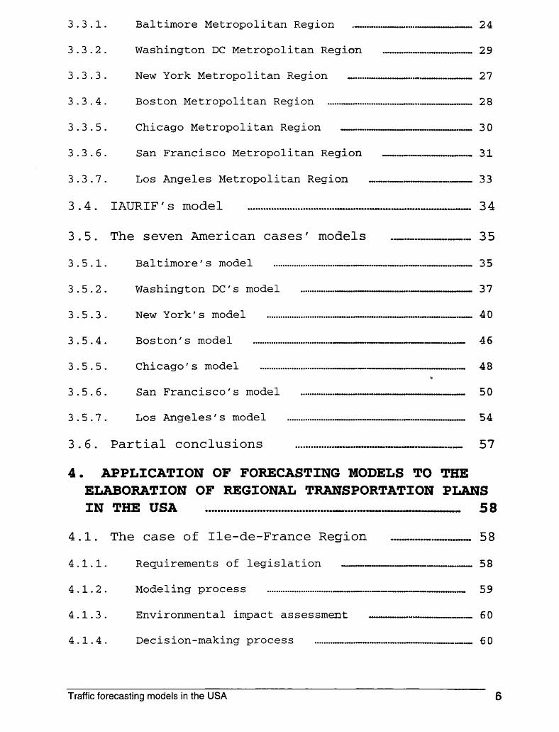
3.3.1.

3.3.2.

3.3.3.

Baltimore Metropolitan Region -... -.- ..--.... .-.---- 24

Washington DC Metropolitan Region .-.-.. ......-.--..- 29

27

3.3.4. Boston Metropolitan Region ......-. ..... 2 8

New York Metropolitan Region - ..........-. .- .... -- . ---

3.3.5. Chicago Metropolitan Region - ..... -.--.- 30

3.3.6. San Francisco Metropolitan Region -.uIIHIIIIIIIIcuIuII 31

3.3.7. Los Angeles Metropolitan Region .. ---- 33

3 . 4 . IAURI F ' s mode 1 ......................*..........-..oo...o.- ....- ~ o ~ o ~ ~ o . ~ o ~ ~ o ~ ~ 3 4

3 . 5 . The seven American cases' models .-.-- 3.5.1. Baltimore s model ........................... -..-.-- ..--..- .--. - 3.5.2. Washington DC . s model ............... UI...-..........-.-..-.-...-.UIIIII

3.5.3. New York / s model -..- ...-.-..-- -.-a-

3.5.4. Bos ton ' s mode 1 .................................. .-- .-.--.- 3.5.5. Chicago . s model .............................. .-- 3.5.6. San Francisco s model ............... -.- ..........-...-.-..-- 3.5.7. Los Angeles . s model ..................... - ........IIIIIUII.. ---..-...

3 . 6 . Partial conclusions ...............-- O I I I I I I I I I I I I I I I I I I .-.-I.-

4 . APPLICATION OF FORECASTING MODELS TO THE

.............................

D

3 5

35

37

40

46

48

50

54

57

ELABORATION OF REGIONAL TRANSPORTATION PLANS IN THE USA ........................................ 0 . . 0 0 0 ~ 0 0 0 ~ ~ a 5 0

4 . 1 . The case of Ile-de-France Region . ............--- 58

4.1.1. Requirements of legislation -......-....-..-....- ....- 58

4.1.2. Modeling process ............................. -- ...-.. .-- P I 59

4.1.3. Environmental impact assessment -..-..-......-..--.. 60

4.1.4. Decision-making process


such as pollution, noise, insecurity) are monetarized (to oppose to a muki-criterion analysis) allows to order the projects and provides the authorities a unique indicator to make their decision. In practice, the DREIF couldn’t calculate this indicator for all projects because of lack of time.

To prepare the Contract of Plan, each agency realizes its own simulations : DREIF, IAURIF and the transit operators (RATP, SNCF). Each one has its own methodology. For example, a traffic study realized by IAURIF defines different scenarios combining different projects, so that you can analyze the interactions between projects. The unique criteria is a first-year rate of return, which takes only into account the time savings but not the disbenefits resulting from increases in environmental impact levels. On the other hand, DREIF has chosen to study each project individually and to apply a multi-criteria analysis, so that the decision-maker can rank himself lhe projects in function of his interests.

The preparation of the Contract of Plan brings about a lot of debates concemingthe assumptions of the data forecasts, the technical aspects of each model, -the methodology of environmental assessment . . . It’s why all planning agencies are aware of the importance to make homogeneous the different models in all points of view. Currently, each one is involved in the process of updating his model.

4.1.3. Environmental impact assessment

In France, you can hear complain about the absence of environment impact criterion in traffic studies. Indeed, the costs of nuisances (“externalities”) such as pollution, noise and insecurity generated by a new infrastructure are not taken into account in a cost-benefit analysis. In particular, there is no air quality analysis in the Master Plan, neither in the Contract of Plan, nor in the Urban Trips Plan. Much effort has been deployed to improve the methodology of environmental impact assessment in a traffic study so far, but in practice when you calculate an internal rate of return or a first year rate of return, the externalities are not integrated. Generally, you make up for this shortcoming with a multi-criteria analysis, in which each criteria can be weighted. Thanks to a GIs, you can also provide a visual presentation of the nuisances as a supplement to the quantitative ranking of projects. Let’s notice that there is a 1995 regulation which imposes a complete environment assessment, but only from 3 to 5 years after the completion of the infrastructure. In this legal procedure, impacts of the new infrastructure must be measured noise, pollution, human beings health, fauna, flora, soil, water, air, climate, . ..

4.1.4. Decision-making process

First of all, let’s point out that the decision-making process in Ile-de-France region is very complex because of the well-known French “bureaucratie” and the implications of the political decisions in the process. Even for a French citizen, it’s seems to be not a1 ways com pre hensi ble.

Traffic forecasting models in the USA .. 80

For the Master Plan, it took about five years for the DREIF to revise it. The main reason was the different shifts of governments during the period 1988-1994 as well as at the level of the Regional Council.

For the Contract of plan, it seems that the orientation of the investments choke is mainly a political decision. The two preponderant criteria are the social interest of a project and the protection of environment. For the next Contract of Plan, the Regional Council has decided to give more attention to the proposition of the “departements” than in the past years. The repattition of investments package between transit and highways projects is fixed a priori, independently of all rational consideration. As far as concerned the roads projects, the priority isn’t given any longer to increase highways capacity but to improve secondary roads. Meanwhile, each agency is working hard to realize traffic studies.

For the Ile-de-France Urban Trips Plan which is elaborated by the Government, the process is really new, It’s similar to the American RTP’s process. Very participatory, it tries to make involved citizens, policy leaderships, professionnals ... A website is devoted to this “PDU”. Http://www.pduidf.orq . The problem with the PDU is that there is no funds devoted to its realization, there are only recommendations, goals, policies and strategies.

4.2. The case of the American metropolitan areas

4.2.1 . Requirements of legislation

ISTEA and TEA 2Il3 have made mandatory for all Metropolitan Planning Organizations to elaborate a Regional Transportation Plan, defined as a twenty year horizon, with a new approach in the planning process. These federal laws wanted to change the way transportation systems are planned. The main goals are the mobitrty improvement and the air cleaning.

These two regulations include many constraints in the elaboration of RTP. They require explicitly : - an intermodal approach, -

- managing demand, - - sensitivity to land use, - - and above all, compliance with the 1990 Clean Air Act : this law requires that metropolitan areas with air quality problems to take a structured, multi-year approach

a financial planning linked to long-term (20-year) corridor and major. project identification,

using innovative financing such as road tolls,

concern for personal, if not regional, equity to access. less use of Single Occupancy Vehicle (SOV),

l3 TEA-21 is the largest public works bill in history. It makes available nearly $218 billion in federal funding for highway, highway safety and transit programs over six years.


to attaining federal clean air standards within established deadlines (the deadfines vary according to the severity of the region’s air pollution problems).

For a project likely some day to be realized, it has to be included in two documents : the long-range RTP and the short-rangeTIP (the Transportation Improvement Program).

The Regional Transportation Plan It includes only those projects and strategies that can be implemented over the planning period with funds that are “reasonably expected to be available.” It describes a financially constrained series of proposed transportation policies, programs and projects that meet the mobility goals and demonstrate that air quality conformity can be met in the future. It is revised and adopted every three years to update policy direction based on changing transportation infrastructure, financial, technological and environmental conditions.

So for each update cycle, all proposals coming from all the actors (individual counties, municipalities, and state and federal agencies, as well as public groups and individuals) are reviewed to determine if they are “regionally significant”. Then the selected projects undergo simulation tests. After this modeling process, a technical analysis and an evaluation of the proposals and considering public comment, the MPO approves final versions of the regional RTP for federal funding.

The Transportation Improvement Program Once the RTP has been endorsed, the TIP shows how portions of the RTP will be implemented over the first six years of the planning period. The TIP is a one or three- year program. It is developed by the MPO in cooperation with state and local officials, regional and local transit operators, and other affected transportation implementing agencies. The program must indicate the priority of projects proposed for implementation during the program period, and must include realistic estimates of total project costs versus the anticipated avalaible resources. The TIP process is a logical follow-up to the implementation of the RTP.

Individual projects in the RTP and TIP are often analyzed in more detail in corridor or sub-area studies. These studies are conducted by state and local agencies in cooperation with the MPO, and in accordance with federal procedures.

The figure below shows the planning process and its relationships both to the management systems and environmental review and control.


#A

Management system performance : Measuredstrategies

Investment strategy

v ‘I

b Metropolitan system planning Corridors/

subarea

Transportation plan

Major investment an a I ys is

Complete environmental review process

Transportation improvement Program

(TI PI

I

I I 1 I ENVIRONMENTAL CONSIDERATIONS <*= implement at ion

4.2.2. Modeling process

In practice, the ultimate goal of a forecasting model is to forecast vehicle.mites traveled (VMT) . These VMT will then be input into an emission model to make the air quality analysis. Transportation planners and engineers hope that that the projected emissions resulting from implementing the projects included in the fcfp and TIP don’t go beyond the US federal standards.

The matter remains that the projects which are simulated concern usually only highways scenarios (capacity expansion or new roads). In theory, MPOs should also simulate the effects of alternative policies (high occupancy vehicles lanes, toll expressways, intermodal facilities, transit-oriented land development, investments in “smart modes”) and calculate the benefit for mobility and the reduction of VMT. Actually, most MPOs have not tested yet these policies with their model, but the RTP document includes even so the proposals (see $4.2.4 for more details).

It’s the paradox : on one hand, the legislation requires that traffic models meet with a lot of new needs, some of them are very difficult to implement. On the other hand,


transportation planners use eventually the model for a very small part. There are probably three reasons : - the air quality conformity is an overwhelming criteria compared to the cost

effectiveness, accessibility or mobility criteria, - the technical difficulty to test the alternative policies, - the lack of time, - mostly, the disinterest from the citizens for the modeling process, so there is no

counterbalance to the technical staff. l4

Let’s notice that everywhere transportation planners and engineers must cope with a frustrating difficulty in the planning process. The question concerns their roles in evaluating projects and in influencing the final decision. It may be that such decisions should be left entirely to the political body or to appointed citizens board. It suffices sometimes that just one individual (a Governor, a mayor), with a strong leadership, can rally everyone behind a transit project that underwent opposition from the mighty State DOT.

4.2.3. Regional Transportation Plans of the seven American .case studies

The seven RTP documents differ by their presentation but they all include more or less the same contents :

Diagnostic of the current situation and forecast of the region with respect to population, labor force, employment and other factors. Discussion of transportation issues facing the region now and in the future. Presentation of different scenarios F)

Presentation of policy goals which can allow to build an intermodal transportation system in compliance with ISTEA and TEA-21 and respond to the future mobility For each policy goal, several objectives are given, and to reach them, several strategies or measures. These strategies focus on managing demand (Intelligent Transportation System, Travel Demand Management) rather than increasing

Listing of the infrastructure projects (improvements and creation) Analysis of the region by travel corridor including recommendation^.'^ Financial analysis designed to determine the region’s ability to fund -the recommendations and determine the funding needs and potential sources of the future. Miscellaneous appendixes : for example, each RTP document has to mciude a chapter that presents the results of an air quality conformity determination; All the assumptions and calculations in each analysis should be included.

‘‘S u p pl y” .

l4 In particular, the forecasting model development is intended to be an opened process with ample opportunity for review and comment both by affected agencies and by selected members of the pubk. Generally the public is not interested in technical aspects. For him, all decision is only political. But it can happen that a citizens board, in which a member is technically skillful, sues a MPO because its traffic model didn’t meet with the legislation requirements (it was the case in California). l5 Some regions like South California are so huge that the MPO (SCAG for example) developed a subregional planning process.


All RTP documents try to emphasize charts and color hot spot maps over narrative. Actually, the RTP is a catalog of all the “most significant” projects, recommendations, policies proposed by all the actors of planning in a region. There is no definition of priority, no ranking. For example, in New York region, the actor New York City highlights only on all surface street system (rehabilitation of bridges, installation of 8200 traffic lights managed by a central computer which adjust cycles to optimize traffic flows) whereas New York State Department of Transportation proposes only highways projects.

http://www. baltometro,ora/look2

http://www. mwcoa .ora/trans/visi on.htmI

020/front.htm_

Most documents (or a summary) are now put on-line in pdf format, so accessible freely to everyone, and you can download them :

Metropolitan area Baltimore

Washing ton

New York

Boston

Chicago

San Francisco

Los Angeles

Name of the RTP ~

“Outlook 2020”

“1997 Update to the financially constrained long-range transportation plan for the National Capital Region “Mobility for the Mi llen iu m”

“The Transportation Plan for the Boston Region” “Destination 2020”

“1 998 Regional Transportation Plan”

“Community Link 21”

Date Nov. 1999

Oct. 1 998

Aug. 1999

April 1997

Aug. 1998

Oct. 1998

April 1998

Address on-line 1

h tt p://www. nvmtc. ordD Ian. ht - ml

http://www.ctps. org/bostonmp o/p lan2000/plan. ht m

htt p ://catsm PO. com/p u bs/d20 20.htm

htt p://www . m tc .ca. govlp roiect s/rt p/rt ptext . h tm

http://www:scaq .ca. gov/rtp/f in al/index. htm

A RTP, intended to be a public document, is almost inevitably an invitation to controversy. For example, in the Baltimore case, when the RTP draft was output, it provoked a lot of controversy. Some public associations studied in details the complete draft and asserted that the RTP was a total failure because in their opinion : - it proposed to spend 2.8 $ billion on new and expanded roads ; - the strategy to << increase transportation choices ’> had no financial back : of a

total of 16$ billion, only 0.1% was devoted to projects which encourage bicycles and walking. it made no proposals that would increase transit ridership, reduce congestion or guide land use planning in a positive way. For example, there is no proposition about road pricing (toll) policy for existing freeways.

-


After protestations, the governor of the Maryland Department of Transportation went back by announcing elimination of $1.5 million in planning money for five road projects. The RTP was then amended in that direction.

4.2.4. Environmental impact assessment

The 1990 CAA required the development of “comprehensive, accurate and current” inventories of each pollutant. Amendments were passed in 1990 to significantly strengthen the law since by 1990 standards for clean air still had not been met in many areas of the USA. Many new threats to public health has also been recognized since the passage of the first CAA legislation in 1963.

For mobile sources (cars), the inventory includes four pollutants : NOx, volatile organic compounds (VOC, precursors to ozone when associated with nitrogen oxydes NOx), CO and small particles (PMI 0). The required emissions inventories were due by November 1992 and had to be updated every three years thereafter. When emissions in a region went below the US emission standards, the region was considered as meeting with the air quality “conformity”. Otherwise it was called a “nonattainment area” for one or many pollutants. So to make a conformity determination, the region’s transportation planners must show that the emissions projected to result from implementation of the RTP and TIP are within the motor vehicle emissions standards. Some States have their own emission standards, which can be more constraining than the US standards, like in California with the “California Clean Air Act”.

In 1992, about 100 metropolitan areas all over the US were designated “severe” nonattainrnent areas for ozone (among them, our seven cases). All MPOs had to take a structured, multi-year approach to attaining federal clean alr standards. Without the “conformity”, these regions risked losing their federal transportation funds. 16

So, all MPOs have incorporated a review of air quality impacts into the transportation planning process and each year, some projects of the Regional Transpottation Plan located in areas with poor air quality are tested. As required by ISTEA and TEA21, the scenarios in the RTP and the TIP have to take into account alternatives to highways projects. In fact, five broad categories of projects, operations, policies or strategies have to be tested in the different scenarios :

1. Transportation Demand Management (TDM), including growth management, congestion pricing and HOV projects,

2. Traffic operational improvements, 3. Public transportation improvements and extensions 4. Intelligent Transportation Systems (ITS) technologies 5. Where necessary, additional system capacity

l6 One of the components of ISTEA was the creation of the Congestion Mitigation and Air Quality (CMAQ) Program. it’s is a federally funded program, continued by TEA21. Six billion dollars were allocated during the period 1991 -1 998 for this program.


No forecasting models can manage to quantify the benefits of VMT and vehicle trip reductions that can be attributed to these strategies.

Technically, another problem arose : the linkage between a traffic model and an emission model didn’t exist. There is an official model that all MPOs have to use. It’s MOBIL, developed by US Environmental Protection Agency (the last version is MOBIL 5A). It requires theoretically a wide range of input parameters, including: vehicle emissions, hourly traffic flow characteristics (vehicle age mix, speed, type mix - car, diesel and gasoline truck, fraction of vehicles in warmed-up or cold condition : all that is utilized to define an average composite emission factor), emission failure rates, vehicle fleet mix, fleet age distribution, topography, roads configuration, meteorology, ambiant air quality, land use, ... 17

No traffic model can today produce all these detailed traffic results. Any practitioner has to make simplification and approximation. Most MPOs have developed an interface from their traffic model to MOBIL. For example, in New York, the interface PPAQ and in south California, the interface DTIM. In practice, these interface call for a lot of “tricks”. For example, if a feedback isn’t made during the four-steps model ensuring that resulted speeds are the most realistic possible, speeds are estimated in an after traffic assignment in the post-processor, using refined speed-volume relationships and final assigned traffic volumes. Post-processed speeds estimated in the validation year are compared with speeds empirically observed during the peak and off-peak periods. These comparisons may be made for typical facilities, for example, by facility clasdarea type category. Based on these comparisons, speed- volume relationships used for speed post-processing are adjusted to obtain reasonable agreement with observed speeds. So you can see how many difficutties you encounter and how much effort you have to spread out in order to ensure that speed estimates are credible and based on a reproducible and logical anamal procedure. Ea

Here also, there can be controversy in the air quality conformity process.- For example, in the case of Baltimore, simulations have shown that the region is now in compliance with the CAM. But these simulations have been made with the 1990 car traffic as input of the emission model. Very recently, Baltimore Metropolitan Council (BMC) realized new simulations with 1996 data. The conclusions seem to be very different : on a typical weekday, emissions coming from cars and trucks in Baltimore region are about I 5 percent greater than previously estimated for all years evaluated. This change results from updating the information about the characteristics of the motor vehicle fleet in the Baltimore region, using more recent 1996 registration data, rather than obsolete 1990 data. The problem is of course not only technical but very touchy and political. It seems that some MPOs have a tactics to avoid controversy about traffic and air quality modeling process : it simply consists not to produce detailed or.-technical documents about it.

For more information about American emission models, see : 17

h tt p ://www . e pa. q ode pa ho m e/mode Is. h t m


4.2.5. The decision-making process

4.2.5.1 . Context

ISTEA gave at the regional level much greater powers to the Metroploitan Planning Organization. It prompts development of the RTP to be a cooperative effort, with participation of all transportation stakeholders and representatives of the public. It tried to break the highways oriented culture imposed by State DOTS. So this process allows everyone to bring its viewpoint about innovative ways and alternatives to increasing highways supply, in order to assure the future sustainability of the region's infrastructure, environment, air quality, economic development, and quality of life. Let's remind that MPO is not a level of government. It's a forum through which the governments responsible for transportation plans, programs or project coordinate their actions. It's actually a sharing of the legal power entrusted in a responsible implementing agency, state or local, with other affected governments. MPOs may have many forms : a Council of Governments (like in Washington), a Metropolitan Planning Commission (like in Baltimore), or an independent transportation planning agency (like the SCAG in Los Angeles) or both all. Typically, there are two bodies : a Policy Committee or board, and a Technical Committee. The Policy Committee is composed of elected officials or local general governments and may or may not include the Governor, commissioner of Transportation, or other state official as a voting member. The Technical Committee consists of the planning, implementation and operating agencies in the region. In addition to the sanctions of funding cutbacks, federal regulations would give the US Environmental Protection Agency the responsibility to implement the CAAA if the MPO fails to reach the federal emissions standards. Thus, a MPO would lose local and regional control over planning decisions. The following schema provides an overview of the theoretical decision-making process :

I b 0

t: I Source : "RTPO transportation planning book" Washington State DOT


4.2.5.2. Participation of the public

ISTEA mandates that a much broader array of population be brought into. the planning process, at all steps of planning because political feasibility is more and more difficult. MPOs have to provide complete, timely information, reasonable public access to technical and policy information, adequate notice of public involvement activities, explicit consideration and response to public input.

All MPOs boards have to set up a structure of subcommittees and advisory pups for the planning process. Each one focus on specific technical and policy areas. You can find for example in the case of Baltimore : - a Technical Committee - a Cooperative Forecasting Group - a Travel Analysis Advisory Group - a Congestion Management Coordinating Group - a Freight Movement Task Force - a Bicycle and Pedestrian Advisory Group - an Interagency Consultation Group - a Transportation Control Measures Advisory Committee - a Land Use Subcommittee

There is generally a monthly meeting for each group, opened to the public.

Usually, to solicit more involved input from the public, the board also creates a kind of citizens advisory committee (CAC). For Baltimore case, the CAC provides a forum for citizens interested in the transportation planning process and provides independent, region-oriented advice to officials on transportation plans. BMC provides support to this committee, including the preparation of agendas, minutes, meeting summaries, the schedules of speakers, the maintenance of mailing lists and the production and distribution of meeting notices. Everyone can also convey directly on Internet through a website devoted to the public.

4.2.5.3. Reality

In practice, the years following the passage of ISTEA were very difficult for tbe implementation of the intermodal planning principles. There were many barriers :

- There was a lack of a regional vision by most partners. The main critic you could hear for each MPO was that the Policy Committee didn’t act on regional interests, only on local interests. Members of the board cooperated with each other behind the scenes to promote their own local interests. The most difficult task within this process is arriving at an understanding of what each city, county, transit authority, State DOT is willing to accomplish and able to afford. The land use is controlled by each county, who wants to keep its prerogatives. So it’s the big problem for a regional planning. Most jurisdictions and transit operators undertake also their own long-range and short-range transportation plans. The work of the MPO is to make the whole compliant.


4 . 2 . 3 .

4 . 2 . 4 .

4 . 2 . 5 .

4.2. The case of the American metropolitan areas . 61 4 . 2 . 1 . Requirements of legislation ............ -...- ........H......-n.-... 6 1

4 . 2 . 2 . Modeling process ............................. -.. ......._. .....IIIIIIIIII n.....II..........--.. 63

RTP of the seven American case studies . -n- 64

Environmental impact assessment --*--.-.-on- 66

The dec is ion-making process -.....onn..o"o.---o--~-o- 6 8

4.3. Comparison between transportation planning process of Ile-de-France region and American met r op o 1 i tan areas ...............................m...............~.....~-....~o~n.~~..~~~.~~ 7 1

5. CONC LUS IONS

A p p endi c e s


- The existing institutional structures of urban transportation planning, funding and delivery systems were a barrier. Very often, there are jurisdictional confusion and inadequate inter-jurisdictional communication. It’s particularly the case for New York. NY Metropolitan area has many more legal jurisdictions as well as more agencies involved in transportation planning. As such, interagency cooperation is that much harder to achieve. As well, jurisdiction areas may not be overlapping. For example, NYMTC area is part of three different areas (“regions”) of NY DOT offices. Interests are also different. NY City DOT is only interested in surface transportation, especially the renovation of bridges.

- Many State DOTs and MPOs continued to plan and operate modes separately. The very strong highway culture remained. Generally, State DOT works with tbe MPO only to ensure that the Regional Transportation Plan and the State Transportation Plan are consistent. So, whereas ISTEA gave much more power to the MPO at the expense of State DOT, it seems that in a lot of cases, the DOT wanted to keep its past prerogatives and was reluctant to relinquish some responsibilities to MPOs.

- The even structure of federal transportation authority doesn’t facilitate. ihe intermodal vision because there is an authority for each mode : Federal Transit Agency (FTA), Federal Highway Agency (FHA), and Federal Railroad Agency (FRA).

- Concerning the citizens participation, you can hear some complaints : At first, they wouldn’t be representative of the population (there are mamiy constituted of elderly people or disabled people or people having no car). Stakeholders who have the strongest self-interest in transportation planning (highway engineers, construction companies, freight haulers and associations representing them) generally do not participate in these proceediqgs. Secondly, they’d be led to think they have input in the transportation planning process but in fact they’d constitute only a “window dressing”, existing mainly because it is required by the federal legislation. The real dealing would be done between the State DOT and elected politicians, county by county. And these elected politicians would try to stay as far as they can from regional issues. Therefore, the public has little to say in real regional issues which are addressed only at the bureaucratic level. Probably this complaint was legitimate the first years after the passage of ISTEA. But gradually, involved citizens have become mature and more organized. You can see that in recent years, the regional dialogue has extended beyond governments and governmental bodies. A number of new regional coalitions, organized by business leaders, public leaders, and special interest groups, are actively engaged in growth and development issues. There are many organized voices in each region who are shaping the growth dialogue, such as developers, homebuilders, local chambers of commerce, environmental groups, and citizens’ organizations. Today they play a more important role than in the beginning in the final decision and can provoke amendments, revisions, corrections of a RTP draft. So we can say that these eight last years of experiences have allow all MPOs, DOTs, transit operators and focal governments to build mutual trust. Today, despite that’s not perfect, there is a better coordination than at the beginning.


4.3. Comparison between transportation planning process of Ile-de-France region and American metropolitan areas

There are five main differences :

1) The link between air quality determination and the regional transportation

In the USA, the elaboration of the RTP and TIP is legally linked with an air qualrty conformity anatysis whereas in France no regulation requires that the Master Plan and the Contract of Plan include an air quality determination. So in the USA a scenario describing a set of highways projects in the long term or in the short term may be rejected because the air quality analysis shows that pollutants emissions don’t meet with federal standards. In France, the reduction of air pollution is the goal of the Regional Urban Trips Plan (PDU) but in this document also there is no quantitative emission determination. The air quality analysis has only to be done a posteriori.

plan

2) Landuse The Master Plan is an official document, elaborated with a regional vision, conformiy to the French “Colbertism” tradition. The land for each project included in the document is resewed unless a revision of the Master Plan takes it out. In the USA, there is no reservation of the land use in the RTP. So The French Master Plan is very powerful.

3) Ranking of projects There is no ranking, no priority in the American RTP. It’s simply a Catalogue of projects and policies. In the other hand the French Master Plan includes a ranking of projects based on an “economic and environmental rate of return”. The elaboration of the American long-range RTP and the elaboration of the French short-range PDU look like. The French PDU is simply a catalogue of policies and measures but there isn’t really any ranking.

4) Financing of projects American federal regulations grant huge amount of money for projects which meet with its requirements. For example ISTEA authorized $25 billion a year (second largest federal-aid program after Medicaid) and TEA-21 $36 billion a year, each one during six years, for highway, highway safety and transit programs’’. So all the planning process is intended to obtain a part of this federal funding. In France, laws don’t precise the amount of State funding. On the other hand, French region is an administrative level and as such, it has its own budget for transportation investments, whereas the region in the USA isn’t an administrative institution.

In particular, the Congestion Mitigation and Air Quality (CMAQ) Improvement Program provides $8.1 billion funding to State and local governments for projects and programs to help meet the requirements of the CAM.

~~~~


5) Citizens participation The American regulation requires the elaboration of the RTP to be participatory. it’s not the case for The French Master Plan. Only the Urban Trips Plan has included in practice the participation of the public during the planning process.

American Metropolitan I le-de- France Areas Region ---

CAAA (1990) + ISTEA (1991) + TEA 21 (1998)

Loi sur I’Etude d’impact a posteriori des infrastructures de transports (1 995) + Loi sur I’Air (1 996)

Regional Transportation Plan SDRIF (RTP) Transportation Improve men t Program (TIP) Congestion Mitigation and Air Quality (CMAQ) Improvement Program County Departement

Contrat de Plan

PDU + PRQA

The following table shows a correspondence between the different plans, regulations and authorities in both countries. The correspondence isn’t perfect as we just have seen.

City

State DOT

Laws

Communes

DREIF

I Long range

MPO

MTA

AMTRAK

I Short range

STP+IAURIF rn

RATP

SNCF

Air quality improvement

governments

Planning agencies

Transit operators

Traffic forecasting models in the USA -. 72

5. CONCLUSIONS

The American federal legislation have required since 1990 significant changes in how State departments of transportation, metropolitan planning organizations, transit operators, and local governments manage transportation planning and programming.

These changes are twofold, both technical and procedural .

. For the technical part, this report has provided an overview of the state-of-the-art and the state-of-the-practice in the field on traffic forecasting models.

As far as concerned the state-of-the-art, three trends emerge from our review :

- -

For the trip demand : evolution towards the activity-based model. For the trip assignment : evolution towards the technique of microsimuiation applied in a metropolitan area incorporating time-sensitive network loadings and departure time choice. For the interfaces with other tools :

GIS for developing and applying transportation forecasting models, combination land usehraff ic models, linkage between traffic model and pollutants emissions model.

- . . . As for the state-of-the practice, the seven case studies have shown a lot of common points between the models. Transportation planners and engineers are still very accustomed to the classical four-steps model. Despite steady updates to try to ensure compliance with federal legislation, the framework of all models remains deeply the classical four-steps model. Indeed, in the prac’tice, a model can easily test a modification of the highway network but still has diff icufties to test demand management policies and to quantify their effects on car trips reduction. It’s even so noteworthy that some MPOs keep on trying to reach the state-of-the- art. Anyway, all MPOs have invested in major improvements of their model for 2000 (now these developments are at various stage of completion). The seven cases’ study show that maintaining a model requires a lot of effort, investment and organization.

For the procedural part, there are mainly two innovations : - The Regional Transportation Plan places new emphasis on managing

demand and land use, on focusing on alternatives modes of transportation, such as transit, walking, and bicycling, ridesharing, and on helping people make smarter travel choices through the application of new ITS technologies. The process has to be fully participatory : any MPO is obliged to support team of interdisciplinary experts to work with elected officials and public, produce a great deal of publicly available information and promote widespread public involvement. This process was designed to generate better decision making, to hold State and MPOs accountable (both politically and legally) .and to achieve better regional coordination.

-


But in the reality, when you analyze financially any RTP document, you find out that the projects of highways expansion still occupy financially the largest part of the plan. So what’s happening in the reality ? This question leads inescapably to political issues.

At first, the elaboration of a Regional Transportation Plan is quite linked with-tbeqair quality determination. Air quality conformity has to be met so that a region receives federal funds for its transportation projects. So it’s the threat of losing federal funds that orients all the transportation planning process in the USA. Though, so far, no traffic model can in a reliable way simulate the effects of alternative policies and evaluate the effects on air quality improvement.

Secondly, the problem doesn’t come only from the shortcomings of the modeling process. The whole transportation planning process can be achieved and led to a consensus (both of officials and public citizens) if there are two political conditions :

- a regional vision of the transportation issues by all local jurisdictions : each crty, county, transit agency shouldn’t focus only on its local issues but develop a broad vision for the region encompassing land use, transportation, economic development, and other quality of life issues. There should be also a greater cooperation and planning coordination between them. Ile-de-France region can be quoted as an example.

- a better involvement of the citizens : actually, the decision-making process seems to center around the State department of transportation’s separate negotiations with officials in each local jurisdiction. These behind-the-scenes negotiations not only shape the long range RTP but also control which projects are elevated from the Regional Transportation Plan to the Transportation Improvement Program. One of the remedies suggested by this report is that if citizens want really to be a counterbalance of the political decision-makers, they have to be more involved in the modeling process because this step has many legal constraints and if these constraints are not addressed, citizens should be aware that they can stop the planning process which wouldn’t suit them.

Traffic forecasting models in the USA ‘ 74

APPENDICES


MEETINGS

The author is grateful to all the persons he met ”. By chronological order :

1) Baltimore Metropolitan Council (BMC)

601 North Howard Street BALTIMORE, MD 21201 Ph : 410-333-1750

Mary Logan, librarian mloqan @ baltometro.orq Gene Brandy, manager of technical services gbandv@ baltometro.orq Matthew de Rouville, Paul Agnello, Victor Henry : transportation planners mderouville @ baltometro.org pagnello @ baltometro.org vhenri 63 baltometro.orq

2) Access svstems : transportation/rehabilitation consultina enaineers & suppliers of access equipments

P.O. BOX 1514 BALTIMORE, MD 21 203 Ph 410-732-61 19

Robert Reuter accessys@ smart.net

3) Metropolitan Washinaton Council of Governments (MWCOG)

777 north Capitol street Washington DC 20002 Ph : 202-962-3200 .

Mark Moran, transportation engineer mmoran @ wwcoaorq

4) Strateaist . Public and aovernment relations

301 West Preston Street BALTIMORE, MD 21201

Amy Blank, lobbyist amy. blank @ hotmail.com

Ph : 41 0-486-0327

5) Federal Transit Authoritv (FTA)

400 Seventh St.,S.W. Washington DC 20590 Ph : 202-366-0371

Tony Yen, Deputy Secretary of research and innovations tonwen @f?a.dot.qov

6) Mawland Office of Planninq

l9 A draft of this report was sent at first on november 30th 1999 to all the met persons. This final report takes into account all the comments and corrections received in december. This report is also written in french.

Traffic forecasting models in the USA . ,76

301 West Preston Street BALTIMORE, MD 21201 Ph : 410 767-4500

Bihui Xu, transportation planner bihui @ mail.op.state.md.us

7) Mawland Department of Transportation (State DOT)

707 Calvert Street, BALTIMORE MD 21 203 Ph : 41 0-545-041 1

Neil J. Pedersen, Director off ice of planning and preliminary engineering NPEDERSEN @ sha.state.md. us

8) National Transportation Library

400 Seventh Str. S.W. Washington DC 20590 librarian @ ntl.bts.qov

9) New York Metropolitan Transportation Council (NYMTC)

1 World Trade Center, 82nd floor New York Ph : 212-938-3341

Tom Schulze, acting director tschulze @gw.dot.state.nv.us Kuo-Ann Chiao manager, models/lTS kchiao@ clw.dot.state.nv.us Sangeeta Bhowmick, senior transportation planner SBHOWMICKG3 gw.dot.state.nv.us

10) New York Department of tranwortation (NYDOT) - Region 11

47-40 21 st Street, Long Island City, N.Y. Ph : 71 8-482-4559

Peter King, supervisor transportation planning and development PKING @ aw.dot.state.nv.us Angelina Foster, staff supervisor [email protected] Mark Tobin, transportation planner mtobin @aw.dot.state.nv.us

1 1 ) Universitv Transportation Research Center

The City College, 137th SVBroadway, New York, New York 10031 Ph 212-650-8050

Pr Robert E. Paaswell, Director paaswell @ tidl s0.enqr.ccnv.cunv.edu Pr Jose Holguin-Veras, assistant professor ihv@ ti-mail.encrr.ccnv.cunv.edu

12) Parsons Brinckerhoff

One Penn Plaza on 34th Street, 2nd floor, New York Ph : 212-465-5259

Pr Sigurd GRAVA, vice president, technical director of planning [email protected]

13) Institute of Public Administration (IPA)

41 1 Lafayette Street New York Ph : 212-982-0306

Bill Shore, consultant bikshore @I nvu.edu

14) New York Citv Department of Transportation (NYCDOT)

40 Worth Street, New York 1001 3 Ph : 21 2-442-7638

Charles N. Ukegbu, Chief Policy & Technology Coordination cukeqbu @dot1 lan.ci.nvc.nv.us

1 5) Central Transportation Planning Staff (CTPS)

State Transportation Building, 10 Park Plaza Suite 21 50 Boston, MA 021 16 Ph : 617-973-7097

Craig Lener, manager of MPO activities cleiner@ ctps.orq

1 6) Massachussets transportation libratv

10 Park Plaza Suite 2150 Boston, MA 021 16 Ph : 617-973-7152

George Sanborn, reference librarian E)

17) Massachussets Institute of Technolow (MITI

MIT 1-1 81, Cambridge MA 021 39 Ph : 61 7-973-7097

Pr Moshe Ben Akiva [email protected]

18) Massachussets Institute of Technoloqv (MITI

MIT 3 Cambridge Center, 2d floor, Cambridge MA 02139 Ph : 617-252-1 116

Hasan Masroor, PHD student masroor@ rnit.edu Didier Burton, research associate in Intelligent Transportation Systems Program dburton @ rnit.edu

19) Chicaao Area Transportation Studv (CATS)

300 West Adams Street Chicago, Illinois, 60606 Ph : 312-793-3456


David A. Zavattero, deputy for operations information @catsrnpo.com or Zavroth @ aol.com

20) Metropolitan Transportation Commission (MTC)

101 Eighth Street, Oakland, California 94607 Ph : 51 0-464-7831

Doug Kimsey, senior planner/analyst Miguel Iglesias, transportation planner/analyst miqlesias @ mtc.ca.gov

dkimsev @ mtc.ca.qov

21) Institute for Transportation Studies (ITS)

University of Berkeley, Berkeley CA 94720- 1720

22) California Deoartment of Transportation (CALTRANS) - District 7

120 S. Spring Street Los Angeles, CA 90012 Ph : 213-897-0362

Raja J. Mitwasi , district Division Chief Planning and Public Transportation Raia Mitwasi @ dot.ca.aov Edwin C. Kampmann, associate transportation planner ekampman @dot.ca.gov Daniel E. Kopulsky, senior transportation planner

23) Southern California Association of Governments (SCAG)

818 West Seventh Street, 12th Floor Los Angeles, CA 90017-3435 0

Ph : 213-236-1889

Naresh Amatya, senior transportation planner amatvaa scaq.ca.qov

24) Department of Planning of Los Anqeles Countv

Hall of records (1 3th floor) 320 West temple street Los Angeles Ph : 213-974 6395

Milan Svitek, chief of Geographical Information Systems Service msviteka plannina.co. la.ca.us Nick Franchino, regional planning assistant nf ranchino@ plannina.co.la.ca.us

25) Universitv of Southern California CUSC) - School of policy, planning and develop men t 3535 S Figueroa St , Los Angeles Ph : 213-740-4473

Pr Genevieve Giuliano giuliano@ almaak.usc.edu

Traffic forecasting models in the USA '79

1 INTRODUCTION

In the field of urban traffic forecasting models, the classical four-steps classical model has been used in most metropolitan areas in the world for a very long time. Tbey were developed in the 196Os, at first to evaluate major highway projects. Any transportation planner or engineer knows its advantages and its limits. Since the beginnings of the 199Os, traffic models have undergone a lot of improvements in the USA and even, new paradigms have appeared. In He-de-France region (Paris region), today, any agency in charge of transportation planning is also involved in a process of improving its traffic model.

The current period is especially interesting to make a review of the research and the practice in the USA. Indeed, three federal laws have recently changed in depth the approach of the transportation planning process in metropolitan areas :

- the Clean Air Act Amendments of 1990 (CAAA) requires -mprovements in air quality and congestion through more efficient transportation and integration of multiples modes,

- the Intermodal Surface Transportation Efficiency Act of 1991 (ISTEA) requires an intermodal approach in the elaboration of the transportation plans, the assessment of potential economic development from transportation infrastructure investment, and a broader participation of the public in the decision-making,

- the Transportation Equity Act for the 21st Century of 1998 (TEA-21) is the successor legislation to the ISTEA and continues most of its programs and policies. *

Before 1991, there was the Federal Transportation Act of 1962 which had during 30 years focused on the roads. The whole transportation planning process in a metropolitan region was organized by the State Department of Transportation (DOT) around road specific planning. Funding programs and policies neither required nor encouraged modal integration of transportation plans. Then, in 1991, Congress proclaimed the end of the interstate highway era and established a new goal for transportation planning and funding "...to develop a National lntemodal Transportation System that is economically efficient, environmentally sound, provides the foundation for the Nation to compete in the global economy and will move people and goods in an energy efficient manner".

ISTEA has also decentralized the decision-making. It gave at the regional level much greater powers to a body called the Metropolitan Planning Organizations (MPO), which previously served only as project organizers.' It has established an exhaustive planning process to include all modes, all levels of governmeni and the public, that must be met and certified in order to receive federal funds. So after 1991, all MPOs had to elaborate a new "Regional Transportation Plan" (RTP).

In 1973, Federal legislation mandated the creation of MPOs in order to create a regional forum to bring together the myriad of federal, state and local governments and agencies to provide for a coordinated and cooperative decision-making process for transportation planning and project funding.

1


26) Los Anaeles Metropolitan Transportation Authoritv (LAMTA)

One Gateway Plaza, MS 99-23-7 Los Angeles, CA 90012-2932 Ph : 213-922-2827

Keith L. Killough, Deputy Executive Officer Countywide Planning KillouqhK @ MTA. NET

27) Oranqe Countv TransDortation Authoritv (OCTA)

550 S. Main street P.O. Box 141 84 Orange, CA 92863-1 584 Ph : 714-560-5579

James Ortner, manager Transit Technical Services JOrtnera octa.net Ronald S. Taira, manager Transportation Analysis Planning and Development rtaira @ octa.net Jeffrey Boberg, GIS transportation analyst jboberg @ octa.net

28) The Baltimore Reaional Partnershb Citizens

Baltimore http://www. balto-reaion-partners.orq/index. htm

Gerry Nelly, independent transportation expert gpneilv@ erols.com


[ l ] :”Baltimore region travel demand model. 1990 validation” - Matthew de Rouviile, Charles M. Baber . March 1998.

[2] : “Draft : FY-99 Models development program for COGflPB travel models. Item’lll E” - Metropolitan Washington Council of Governments. June 30, 1999.

[3] : “Transportation models and data initiative . Technical memorandum No 1.22. Final model structure and framework” - Parsons Brinckerhoff Quade for New York Metropolitan Transportation Council. June 25, 1 997.

[4] : “Central artery project : traffic study” - Central Transportation Planning Staff for Boston Metropolitan Planning Organization. April 1987.

[5] : “Unified planning work program. Fiscal year 2000” - Central Transportation Planning Staff for Boston Metropolitan Planning Organization. September 8, 1999.

[6] : “2020 regional transportation plan” - Chicago Area Transportation Study. August 1998.

[7] : << Travel demand modeling for the conformity process in Northeastern lllinois w - Appendix B. Chicago Area Transportation Study. November 1997.

[8] : “San Francisco Bay area 1990 Travel model development project. Compilation of technical memoranda. Volume VI” - Metropolitan Transportation Council. April 1997,

[9] : “Demand Transportation Model : the mode choice model. Projects’ - Southern California Association of Governments , May 1997.

[IO] : “Comparison of OCTAM 2.8 and OCTAM 3.0” - Orange County Transportation Authority.

[l 11 : “Le modele de trafic de I’IAURIF’ - Dany Nguyen-Luong . May 1997.

[12] : “Discrete choice analysis : theory and application to travel demand” - M. Ben- Akiva and S. Lerman . MIT press. 1985.

[ 131 : “Activity based disaggregate travel demand model system with daily actnnty schedules” - Moshe E. Ben-Akiva and John L. Bowman. In “Transportation Research Board”. 1995.

[14] : “Multinomial probit, the theory and its application to demand forecasting’? - Carlos Daganzo. 1979.

[ E ] : “The dogit model” - M. Gaudty and M. Dagenais. In “Transportation Researcb Board”. 136, 105-1 11. 1979.


[ 1 61 : “Understanding Heggie . 1983.

[I71 : “Activity based Timmermans. 1999.

travel behavior” - P.M. Jones, M.C. Dix, M.I. Clarke, 1.G.

approaches to travel analysis” - Dick Ettema and Harry

[I 81 : “TRANSIMS-LANL-1 .O- Ovewiew” - Los Alamos Laboratory . May 1999.

[I 91 : “Demand model estimation and validation” - Daniel McFadden, Antti P.TaMie . June 1977.

[20] : “A Technical review of urban land use-transportation models as tools for evaluating vehicle travel reduction strategies” - Franck Southworth. Oak Ridge National Laboratory. July 1995.

[21] : “A rnulticriteria method for transportation investment planning” - Genevieve Giuliano . Transportation Research 19A:29B41. 1986.

[22] : “ Scenario Analyses for The Chicago Region with a Sketch Planning Model of Origin-Destination Mode and Route Choice. Final Report” - D.E. Boyce, M. Tatmeni, and Y. Zhang . Illinois Dept. of Transportation. 1992.

[23] : “Incorporating feedback in travel forecasting models : methods, pitfalls and common concerns” - Comsis Corp. For FHA. TMlP Program. March 1996.

Traffic forecasting models in the USA ..%2

The elaboration of a regional transportation plan requires the-use of forecasting models. For this purpose, traffic engineers and transportation planners couldn’t afford to keep on using simply their old traffic forecasting model. ISTEA requires that traffic model have to meet with four complex capabilities :

1. The model must be multimodal : it must handle highway and transif analyses equally well.

2. It must allow to analyze the interrelation between land use and transportation. 3. It must satisfy regional needs for air quality assessment. 4. It must be sufficiently flexible to support adaptation to other analysis, such as the

evaluation of Traffic Demand Management (TDM) strategies and the High- occupancy-vehicle (HOV) lanes.

So all MPOs have been involved since 1991 in a process of updating their model, It’s the good time to learn about American practices. Moreover, the more and more powerful computer resources make now feasible some analytical approaches proposed by researchers for a long time that were impossible to implement just a few years ago.

This report will deal at first with two aspects :

“The state-of-the-art” : the research field has been very prolific for thirty years in the USA, as you can see in the numerous transportation research reviews. What are the last technical innovations proposed by researchers ? “The state-of-the-practice” : what are the models used in practice today ? The case of Ile-de-France will be at first evoked quickly. Then seven cases will be studied : Baltimore, Washington DC, New York, Boston, Chicago, San Francisco and Los Angeles. These cities are not representative of the American cities but they will provide a state-of-the-practice in the United States at the close of the twentieth century.

In a third part, we will see how each MPO has applied its traffic model to elaborate its long-range regional transportation plan. But in the whole transportation planning process, the modeling is a small part. We will try to evaluate the importance of traffic studies in the decision-making process.

The American term “transit” is equivalent to the British term “public transportation”, 2


traffic forecasting models in the usa · traffic forecasting models in the usa ... environmental...

Documents