traffic management strategies for merge area in rural

,---------------------- ---· ------ --------·-------------- --- ----- - --

TAl Io8p 97-12a

TRAFFIC MANAGEMENT STRATEGIES FOR

MERGE AREAS IN RuRAL INTERSTATE WoRK ZoNES

CTRE Management Project 97-12

jULY 1999

- ---- --,

' I<lWADEPT.OFTRANSP~R~ATION. \ .! LIDRARY '•

800LINCOLNWAY . \

Center For Transportation Research and Education

IOWA STATE UNIVERSITY

Iowa Department of Transportation

AMES, IOWA 50010 : - _.::__.~----.

- - - - - - - - - - - -- - -- - - - ---------c-------------- -- - - - - - - ---

TRAFFIC MANAGEMENT STRATEGIES FOR

MERGE AREAS IN RuRAL INTERSTATE WoRK ZoNES

Principal Investigator Tom Maze

Director of CTRE Professor of Civil and Construction Engineering

Iowa State University

Graduate Assistants Steve Dale Schrock Kera VanDerHorst

Iowa State University

Preparation of this report was financed in part through funds provided by the Iowa Department of Transportation

through its research management agreement with the Center for Transportation Research and Education,

CTRE Management Project 97-12, and through funds provided by

Mid-America Transportation Center, University of Nebraska-Lincoln.

Center for Transportation Research and Education Iowa State University

Iowa State University Research Park 2625 North Loop Drive, Suite 2100

Ames, lA 5001 0-861 5 Telephone: 515-294-8103

Fax: 515-294-0467 http:/ /www.ctre. iastate.edu

July 1999

TABLE OF CONTENTS PAGE

EXECUTIVE SUMMARY . . . . . . . . . . . . . . . . . . . . . . . . . . . . . . . . . . . . . . . . . . . . . . . . . . . . . ii ACKNOWLEDGMENTS ...................................................... iii CHAPTER 1: INTRODUCTION ................................................. 1

PHASE 1: LITERATURE REVIEW ........................................ 2 PHASE 2: DATA COLLECTION .......................................... 2 PHASE3: DATA ANALYSIS .............................................. 3 PHASE 4: WORK ZONE SIMULATION TOOL ............................. 3

CHAPTER 2: LITERATURE REVIEW ........................................... 5 CAPACITY, FLOW, AND DELAY ......................................... 5

Queuing Behavior ................................................. 12 ESTIMATING CAPACITY OF INTERSTATE LANE CLOSURES ........... 17

What Do Other State Departments of Transportation Do? ............. 19 INNOVATIVE WORK ZONE APPLICATIONS OF TECHNOLOGY ......... 21

Regional, Statewide, and Multistate Systems .......................... 23 Traffic Management System in the Region of the Work Zone ........... 24 Single Function ITS Work Zone Related Systems ..................... 25

CHAPTER CONCLUSIONS ............................................. 28 CHAPTER3: SITE SELECTION ............................................... 31

CRITERIA FOR A SUITABLE LOCATION ............................... 32 SELECTION OF SITE CRITERIA ........................................ 32 SUMMARY ............................................................ 33

CHAPTER 4: MOBILE TRAFFIC DATA COLLECTION OPERATIONS ........... 37 FIELD DATA COLLECTION METHODOLOGY ... : ..... .' ................ 38

Traffic Video Collection ............................................ 38 Queue Length Data Collection ...................................... 40

RESULTS OF SUMMER DATA COLLECTION ........................... 41 Limitations of Data Collection at the Davenport Location .. ~ ........... 42

SUMMARY ............................................................ 43 CHAPTER 5: LABORATORY DATA REDUCTION .............................. 45

AUTOSCOPE DATA REDUCTION ...................................... 45 SUMMARY ............................................................ 46

CHAPTER 6: ANALYSIS AND RESULTS .................................. ; .... 49 CAPACITY ............................................................ 49

Determining Capacity ............................................. 49 QUEUE LENGTH ......................................... : ............ 53

Behavior of the Upstream End of the Queues ......................... 57 CHAPTER 7: CONCLUSIONS AND RECOMMENDATIONS ..................... 61

WORK ZONE CAPACITY ............................................... 61 WORK ZONE DELAY COST IMPOSED ON MOTORISTS ................. 62

REFERENCES ................................................................ 65 .

Traffic management Strategies for Merge Areas in Rural Interstate Work Zones

TABLE OF TABLES

Table 2-1 Results of State Transportation Agency Interviews ..................... 20 Table 3-1 Criteria for a Suitable Data Collection Site ............................ 32 Table 3-2 1998 Merge Area Study Candidate Projects ........................... 34 Table 3-3 Reasons for Elimination of Potential Data Collection Sites .............. 35 Table 3-4 Suitable Data Collection Sites ....................................... 35 Table 4-1 Field Data Collection Trailer Component Parts ........................ 37 Table 4-2 Summary of Data Collection Dates and Locations ...................... 42 Table 6-1 Observed Unconverted Traffic Volumes .............................. 49 Table 6-2 Observed Unconverted Traffic Percentages ........................... 49 Table 6-3 Observed Capacity Values during Free-flow Conditions ................ 53 Table 6-4 Observed Traffic Characteristics Under Queued Conditions ............ 53 Table 6-5 Economic User Delay Costs for Observed Queues ...................... 57

Traffic Management Strategies for Merge Areas in Rural Interstate Work Zones

TABLE OF FIGURES

Figure 2-1, Linear Speed Density Relationship .................................. 7 Figure 2-2, Flow-Density Relationship .......................................... 7 Figure 2-3, Speed-Flow' Relationship ........................................... 8 Figure 2-4, Speed-Flow Relationship Taken From 1985 Highway Capacity Manual ... 9 . Fig~re 2-5, Three Regime Speed-flow,Relationship .............................. 10 Figure 2-6, Example of Deterministic Queueing Theory .......................... 13 Figure 2-7, Backward Forming Shockwave .................................... 15 Figure 2-8, Forward Forming Shockwave ...................................... 15 Figure 2-9, Queue Length Data Collection Schematic ............................ 16 Figure 2-10, Conceptual Drawing of Indiana Lane Merge System ................. 27 Figure 4-1, Field Data Collection Trailer in Operation ........................... 38 Figure 4-2, View of Electronic Equipment in a Data Collection Trailer ............ 39 Figure 4-3, Typical Location of Field Data Collection Trailer ..................... 39 Figure 4-4, Typical Placement of a Calibration Grid ............................ 41 Figure 4-5, Example of Collection of Queue-Length Data ........................ 41 Figure 4-6; Location of the Data Collection Site at Davenport ........... · ......... 43 Figure 5-1, Example of Autoscope Supervisor Calibration Grid ................... 46 Figure 5-2, Example of Virtual Detectors Placed over Video Image ................ 47 Figure 6-1, Analysis ofTen Highest Converted Free Flow Values, 7/2/98 ........... 51 Figure 6-2, Analysis ofTen Highest Converted Free Flow Values, 7/10/98 .......... ·51 Figure 6-3, Traffic Volumes and Speeds, 8/7/98 .................. · ............... 52 Figure 6-4, Traffic Volumes and Speeds, 6/19/98 ................................ 52 Figure 6-5, Queue Length on 6/19/98 .......................................... 54 Figure 6-6, Queue Length on 7/2/98 .................................... ; ...... 54 Figure 6-7, Queue Length on 7/10/98 .......................................... 55 Figure 6-8, Queue Length on 817/98 ........................................... 55 Figure 6-9, Speed Change of End of Queue, 6/19/98 ............................. 58 Figure 6-10, Speed Change of End of Queue, 7/02/98 ............................ 58 Figure 6-11, Speed Change of End of Queue, 7/10/98 ............................ 59 Figure 6-12, Speed Change of End of Queue, 8/7/98 ............................. 59 Figure 7-1, Using Capacity Values to Determine if Congestion Might Occur ....... 62

Traffic Management Strategies for Merge Areas in Rural Interstate Work Zones

EXECUTTVES~RY

The Iowa Department of Transportation, like many other state transportation agencies, is experiencing growing congestion and traffic delays in work zones on rural interstate highways. The congestion results in unproductive and wasteful delays for both motorists and commercial vehicles. It also results in hazardous conditions where vehicle stopped in queues on rural interstate highways are being approached by vehicles upstream at very high speeds. The delays also result in driver frustration, making some drivers willing to take unsafe risks in an effort to bypass delays. To reduce the safety hazards and unproductive delays of congested rural interstate work zones, the Iowa Department of Transportation would like to improve its traffic management strategies at these locations. '

Applying better management practices requires knowledge of the traffic flow properties and driver behavior in and around work zones, and knowledge of possible management strategies. The project reported here and in a companion report documents research which seeks to better understand traffic flow behavior at rural interstate highway work zones and to estimate the traffic carrying capacity of work zone lane closures. In addition, this document also reports on technology available to better manage traffic in and around work zones.

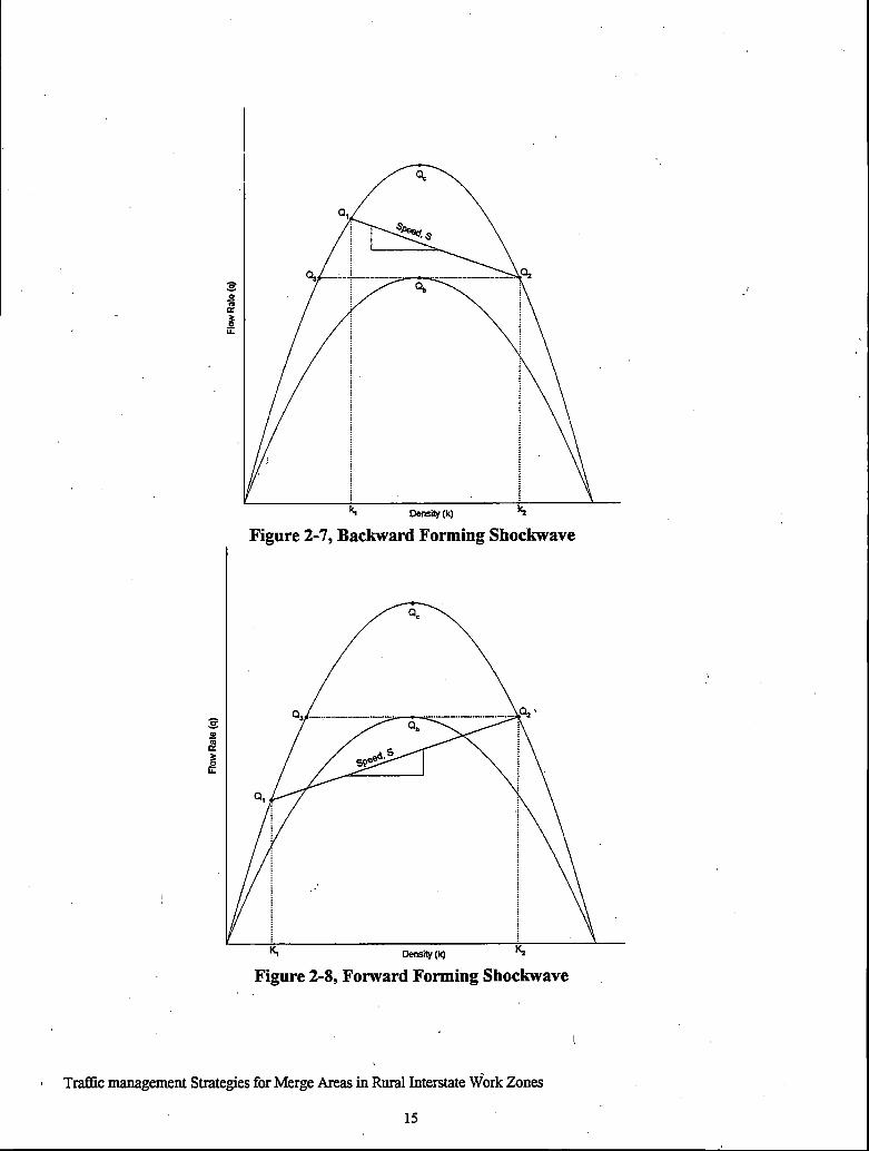
Traffic performance data were collected at an Iowa interstate highway work zone using traffic data collection trailers. These trailers were constructed as part of this project and are jointly owned by the Iowa Department of Transportation and the Center for Transportation Research and Education. They use a pneumatic mast to hoist video cameras 30 feet above the pavement's surface where the cameras collect video of traffic operations. Videos are then turned into traffic flow performance data using image processing technology.

Through the use of the data collection trailers, traffic performance data were collected at one work zone on Interstate Highway 80 where two lanes are reduced to one lane. Through analysis of these data, a work zone lane closure capacity of 1,374 to 1,630 passenger cars equivalents per hour was estimated.

The companion report to this report documents the development of a work zone simulation model with an animation interface. The simulation model provides a platform for the analysis of traffic behavior in the merge area and the analysis of delays under varying traffic demands.


ACKNOWLEDGMENTS

The project reported in this report was funded~ in part, by financial support of the Iowa Department of Transportation through its management agreement with Iowa State University.

, Parts of the project were also supported by the Mid-America Transportation Center at the University ofNebraska-Lincoln. We very much appreciate the opportunity to conduct the research reported. We are also grateful for the advice and assistance provided by the members of the project's technical advisory committee at the Iowa Department of Transportation. The committee includes Dan Sprengeler, Steve Gent, Mark Bortle, and Dan Houston. In addition, we very much appreciate the technical advice we were given by members of the staff of the Mid-America Transportation Center who helped in the development of our data collection trailers and in data collection procedures. ,


1.

CHAPTER 1: INTRODUCTION

The Iowa Department of Transportation (Iowa DOT) sponsored the Center for Transportation Research and Education (CTRE) conduct of research on the capacity and driver merge behavior at Interstate work zone merge areas. The prmciple goal of this research is to determine the traffic capacity at work zone locations where two lanes of traffic are reduced to one (lane closure). Reducing two traffic lanes to one in each direction is the typical method of channeling traffic into a work zone on Iowa's rural Interstate system. When traffic volumes exceed the capacity of these merge points, the resulting congestion can lead to the formation of queues, which result in delays and increases the potential for traffic crashes. Successful implementation of work zone improvements at locations where congestion is expected will provide a benefit to motorists through reduced delays and increased safety.

The research project was conducted in four phases: a literature review, the collection of traffic data at work zone merge areas, the analysis of this data, and the development of a computer simulation tool to model traffic at merge areas.

PHASE 1: LITERATURE REVIEW

First, a literature review was conducted to determine what research had been previously performed to estimate the traffic-carrying capacity of work zone lane closures and to analyze the behavior of traffic in work zones. Additionally, other state departments of transportation were contacted to determine current work zone traffic management methods. This literature review and a review of current practices are provided in Chapter 2.

Much of the current body of literature was generated from a number of research projects spons_ored by the Texas Department of Transportation (DOT) and conducted by the Texas Transportation Institute during the late 1970s and 1980s. This work is the basis of the procedures for determining interstate highway work zone capacities used in the Highway Capacity Manual. In the last ti.vo years, there has been renewed interest in this topic and a few other research projects have recently been conducted on interstate work zone capacity, traffic safety in work zones, and driver merging behavior. The most significant of these past and ongoing projects are ones sponsored by the Indiana and North Carolina Departments of Transportation (DOTS). Other related projects have been initiated by the Nebraska Department ofRo.ads and the state departments of transportation in Iowa (in addition to this project), Kansas, and Missouri.

Another portion of the literature review involved a review oflntelligent Transportation Systems (ITS) that are used to manage traffic in and around work zones and to advise motorists of work zone-related delays. Applications ofiTS generally have two components, the roadside field devices and the deskside databases, algorithms and processes used to manage and control traffic. To date, work zone applications ofiTS technology have focused on the roadside and very little has been conducted to develop desks~de procedures and processes. Roadside technology . applied to work zones can be broken into three levels. First, there are systems which manage traffic and provide motorist information in and around work zones as simply another traveler information function of the system. These include regional or statewide traffic management and


1

traveler information systems. At the second level, there are systems which seek to control traffic in and around the work zones through a number of strategies. These systems might include motorist information upstream of a work zone (e.g., using a changeable message sign), congestion management procedures (e.g., highway advisory radio recommending diversion routing), and surveillance for detection and removal of incidents. Lastly, there is technology which focuses on only one function, e.g., slowing motorists in work zone areas. A number of automated roadside devices are currently available to manage traffic at work zones and more are being introduced. To manage and control work zone traffic the Iowa DOT currently utilizes manual flaggers, fixed signs, changeable message signs; the internet, and highway advisory radio to provide motorists with information and control traffic in work zones. New automated field devices have been and are currently being developed that increase safety,' convey real-time information to motorists, and provide information to traffic managers. This project included a review of some of these emerging technologies. A discussion of selected technology is presented in Chapter 2.

PHASE 2: DATA COLLECTION

The second phase of this project is to collect actual traffic data at merge areas under varying traffic volumes to observe traffic at the moment that capacity is reached and queues begin to form. Two mobile data collection units (trailers) were developed to capture these data.

Throughout this project, CTRE worked closely with the Iowa DOT for equipment support and approval of the field procedures. Additionally, CTRE coordinated with the lllinois DOT to collect traffic data on highways in that state. The University ofNebraska at Lincoln was a valuable resource during this project, providing CTRE staffwith guidance in developing a traffic data collection methodology and technical guidance in the use of mobile video surveillance equipment.

CTRE staff also worked closely with Iowa DOT engineers to develop a data collection procedure allowing data to be easily collected. Additionally, the procedure could be accomplished without requiring personnel to enter open lanes of traffic, and that would not compromise the safety of motorists in the event they left the roadway. The Iowa DOT, in conjunction with Iowa State University, purchased and assembled two mobile video trailers with the ability to raise video cameras above the roadway to record traffic.

The data collection for this project was originally planned for the 1997 construction season. However, due to delays in assembling the data collection equipment, no useable data were collected that year. Field operations were conducted throughout the 1998 construction season. Based on the site selection process established in Chapter 4, many potential construction projects were eliminated as possible data collection sites. In order to maximize the potential for observing a work zone at capacity, field data collection was limited to only two locations during the 1998 construction season. Ultimately, only one location experienced congestion. All useable capacity data analyzed in this report was collected at th~ Interstate 80 reconstruction project near the US 61 interchange in Davenport, Iowa. A summary of the data collection experiences is provided in Chapter 5.


. 2

PHASE 3: DATA ANALYSIS

After traffic video was recorded in the field, it was brought back to the Autoscope Laboratory at CTRE to convert the video images to quantifiable data. This process is described in Chapter 7. The data were analyzed to determine capacity of the work zone merge area. These data are also used to develop estimates of the costs imposed on user through the delays resulting from lane closures.

Conclusions and recommendations based on the observed traffic conditions at work zone merge areas are made in Chapter 8. The range of capacity values of the work zone studied in this project are presented, along with recommendations on hovv this range of values could be used by· the Iowa DOT to assist in planning future work zones. Insights are drawn concerning the frequency of aggressive motorists. Finally, a recommendation for improved traffic management planning is offered that may reduce driver frustration during congestion at merge areas.

PHASE 4: WORK ZONE SIMULATION TOOL

A computer simulation tool has been developed at CTRE using the ARENA simulation package. The purpose of the simulation .model is to help Iowa DOT staffbetter understand traffic behavior at a work zone lane closure. The simulation package will allow the user to view traffic conditions under varying traffic volume levels, and determine estimates of the queue length and delay. This tool and its supporting documentation is delivered in a companion report.

Traffic management Strategies for Merge .At'eas in Rural Interstate Work ZOnes

3


4

CHAPTER 2: LITERATURE REVIEW

The purpose of this project was to assist the Iowa DOT in understanding traffic capacities of freeway work zone merge points and the resulting motorist delays at various rates of traffic flow. To understand the relationship between one system parameter (capacity) and the other two system variables (flow and delay) requires knowledge of the traffic behavior in and around the merge point. To do this, the first part of this chapter introduces the fundamental concepts of facility capacity, traffic flow, and delay. Later, these concepts will be used as a foundation for a more thorough examination of traffic behavior in the work zone. The last part of this chapter examines advanced technology being applied to better manage traffic and inform drivers of travel conditions in and around work zones.

CAPACITY, FLOW, AND DELAY

Flow is often referred to as traffic demand. It involves the number of vehicles being processed or arriving to be processed through the merge point per unit of time (usually identified as the variable q). The typical units of flow are in vehicles per hour, vehicle per hour per lane, or passenger car equivalents per hour. Passenger car equivalents take into account the increased impact oflarger vehicles (in comparison to a passenger car) and the volume of trucks, buses, and recreational vehicles is factored up to account for their larger impact.

Flow is a function of vehicle density (the number ofvehicles per length of road) and the speed of the traffic flow. Vehicle density is typically noted as the variable k and is reported in vehicles per mile or vehicles per lane per mile. Vehicle speed is usually noted as the variable u j

and is reported in miles per hour: Equation 2-1 is the relationship used to estimate flow. In the flow-density-speed relationship

1We always refer to the space-mean-speed, as opposed to

time-mean-speed. The Highway Capacity Manual defines space-mean-speed as "the average speed of the traffic stream computed as the length of the highway segment divided by the average travel time of the vehicles to traverse the segment."(!) The manual defines time-mean-speed as "the arithmetic average of individual vehicle speeds passing a point on a roadway or lane." The equation used to estimate space-mean-speed is shown in Equation 2-2. Density is the inverse of the vehicle headway (distance from front bumper to front bumper of consecutive vehicles) and the equation to estimate the density is in Equation 2-3. The relationship between flow, density, and speed is expressed below in Equation 2-4. ·

., a=~ .. ' (2-1)

(2-2)

k=~ .. ' (2-3)

q=uk (2-4)


5

Where: q =the volume for n vehicles passing a point during time t. u = the space-mean speed of n vehicles over distance 1. t = Hti(h) +t:;:(h) + · · · +tnOn)] k = the density of n vehicles over a distance l.

The terminology for flow on a highway is very similar to the terminology for fluid flow. However, there is one significant difference between the study of the mechanics of most fluids and traffic. Specifically~ most fluids are· treated as being incompressible. Because of the relationship expressed in Equation 2-4, both flow and speed are dependent on density which is very different than the physical relationship for flow of an incompressible fluid. ·

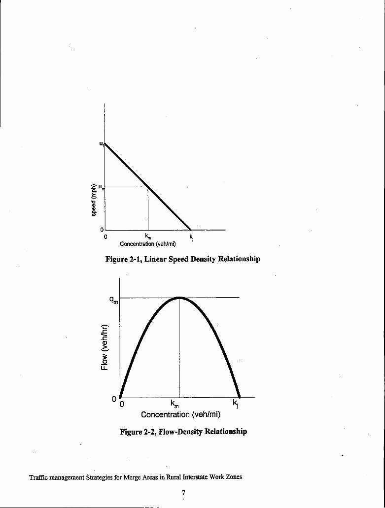
Bruce Greenshields studied the relationship between flow, speed, and density and published his theory on the relationship between the three variables in 1934.(2) Greenshields postulated that the relationship between speed and density was linear, as shown in Figure 2-1. Although many have postulated and estimated different functional fonns for this relationship since Greenshields, the elegance of his original work lies in its simplicity. Shown in Figure 2-1 are the freeflow speed (u;) where density is zero, and jam density (ki) where speed decreases to zero. The area under the curve at any point along the curve between jam density and freeflow speed provides the flow (q) for that density and speed. The line in Figure 2-1 can be defined by Equation 2-5. By substituting Equation 2-4 into Equation 2-5, the relationship between flow and density is derived and the parabolic flow-density relationship is written in Equation 2-6 and shown in Figure 2-2. In Equation 2-7 is the most commonly cited traffic flow relationship. The relationship between speed is flow is shown in Figure 2-3.

(2-5)

(2-6)

. k( u~ \ a = . .,u--) 1 ~J .... -. u, (2-7)


6

. -----------------------------------------------------------------~

o~------~--------~--------0. ~

Concentration (veh/mi)

Figure 2-1, Linear Speed Density Relationship

"C' .c -.c (]) > -

~ Concentration (veh/mi)

Figure 2-2, Flow-Density Relationship


7

0 Flow (veh/hr)

Figure 2-3, Speed-Flow Relationship

Greenshields speed-flow relationship (Figure 2-3) has received the most attention and is most commonly cited in the traffic engineering literature. Prior to the 1994 Highway Capacity Manual, the speed-flow relationship based on Greenshields' model was used as a framework for representing level of service on highways. When a highway is operating at the upper end of this curve, motorists are free to maneuver. As the flow increases, the highway becomes more crowded, individual motorists have less ability to maneuver, and the level of service decreases until the flow reaches the maximum (qm).

Greenshields' representation of the flow-speed-density relationship is elegant and simplistic. It uses a single function to represent the entire range of operation (otherwise known as a single regime relationship). Others have used other functional forms (non-linear equations) to model the speed-flow-density relationship. In Equations 2-8, 2-9, and 2-10, alternative single regime models developed by Greenberg, Underwood, and Drake, respectively, are shown. (3),(4),(5)

(2-8)

/...,. ' z.s = Urn€ l T.;) (2-9)

(2-10)


8

Where: 'lim= The speed at the maximum flow Uf' =The mean free-flow speed (speed at low volumes) ~- = Jam density (where flow and speed are zero) km =The density corresponding to the maximum flow/

In the 1960s, researchers began to note that these single regime models did not model traffic flow equally well across all levels of traffic density. For example, Greenberg's model represents behavior better at high traffic densities while Underwood's model is a better representation of traffic behavior at lower densities.(6) This illustrates the need for multipleregime models where different functions are used to represent different portions of the speed-flow-density continuum.

The conventional thought on speed-flow relationships through the 1985 edition of the highway capacity was a single regime curve. The fairly standard relationship between speed and flow is shown Figure 2-4, which is taken from chapter 3 of the 1985 manual. In the late 1980s and early 1990s research was conducted to analyze this relationship and create a more realistic

2 4 6 II ·;o. 12 1!1 · is '·J& 20 YOLI"'IICOpcplo) lOll CO.:H 1=1 ·(1)!11 .IQSl IO.Sl . !07'l . to.al 10•1 CI.Ol we !lOtto••

model of the speed-flow relationship. Figure 2-4, Speed-Flow Relationship Taken from 1985 Hi&hway Capacity Manual

Hall, Hurdle, and Banks published a paper which identified three distinct portions of the speed-flow relationship. 1(7) A "generalization" of this relationship is shown in Figure 2-5. The upper portion of the curve (the uncongested portion) is relatively flat. The 1990 interim Highway Capacity Manual first adopted the rather flat upper portion of the curve. The flatness indicates that speeds diminished very little until the capacity of the facility is reached. The 1994 Highway Capacity Manual fully embraces the relationship of relatively constant speeds while flow increases

1 This text is paraphrased from Hall, F.L., "Traffic Stream Characteristics," Chapter 2 of Update of Traffic Flow Theory, Prepared for the Transportation Research Board Committee on Traffic Flow Theory and Characteristics.


9

in the uncongested portions of the speed-flow. For example, in chapter 3, for four-lane freeways, the manual shows speed remaining constant until the flow reaches two-thirds of capacity and speeds only dropping from free flow speed (at 65 miles per hour) to 56 miles per hour at capacity, a reduction in speed ofl4 percent as opposed to the 50 percent drop in speed identified in Greenshields' relationships. In Figure 2-5, there are really three distinct portions of the speed flow relationship; uncongested, queue discharge (free flow recovery and sometimes called capacity flow), and congested (with queuing). Other researchers have found similar findings regarding the speed-flow relationship including Banks, Hall, and Hall, Chin and May, Wemple, Morris and May, Agyamang-Duah, and Hall, and Ringert and Urbanik.(8),(9),(10),(11),(12),(13) Findings of all of these researchers support the notion that speeds remain fairly constant even at quite high flow rates. Most of the research that has been done to this point, however, has focused on the shape of the uncongested flow portion of the curve.(14)

"C CD CD c. (/)

Congested Flow

Flow

Figure 2-5, Three Regime Speed-flow Relationship

Queue Discharge

A common aspect of the movement along the curve from uncongested to congested is capacity drop. In other words, immediately before the flow breakdown occurs the flow rate is greater than after a flow breakdown. Therefore, when the queuing condition is reached, a capacity reduction (or drop) occurs.(15),(16) The capacity drop is due to turbulence in the traffic flow that results after a breakdown. Later in this report, we present the data we observed at a freeway work zone in Iowa. We did not observe a capacity drop. Although a capacity drop was not observed in the Iowa data, a similar study of freeway work zones conducted in North

Traffic management Strategies for Merge Areas in Runil Interstate Work Zones

10

Carolina found a precipitous capacity drop: In the North Carolina study, capacity at a lane closure merge point dropped from 1210 vehicles per hour to 1065 vehicle per hour (a 12 percent capacity drop) when the traffic arriving exceed the traffic discharge and flow breakdown occurred. ( 17) Other research has found that a capacity drop of approximately six percent should be expected once a flow breakdown has occurred and queuing is established. To think of this another way, Hall and Agyemang-Duah point out that a six percent "bonus" is available if queues can be delayed. ( 16) ·

Work conducted in Indiana by Jiang to characterize flow-density relationships at saturated work zones on interstate highways also found both a speed and a traffic flow drop when a queue begins to form at lane closures upstream from work zones.(18) Jiang further suggests that after a queue forms, the maximum flow of the work zone should not be thought of as the capacity ofthe facility. He states that the capacity of the facility should be measured immediately before the queue forms. After the queue forms, Jiang suggests that the flow rate being observed is really the queue-discharge rate, which will usually be smaller than the capacity before a queue forms (due to the drop). Jiang further found that the difference in flow rate between the capacity and the queue-discharge rate does vary by the type of lane closure. The smallest difference results when there is a lane crossover and discharge flow is being measured for the traffic which crosses the median (1.6 percent flow rate drop). The flow drop is much greater in the direction that does not crossover the median but flows in the opposite direction (20.2 percent drop). When there is a right lane closure and the left lane continues, the flow rate drop is greatest, dropping by 20.9 percent. When the left lane is closed and the right lane continues the drop is 9. 7 percent. What this suggests is the flow rate bonus of delaying or avoiding a queue (by diverting traffic) can be quite significant and varies with the approach configuration. The difference in the capacity drop from a right lane closure and from a left lane closure is due to more traffic having to merge from right to left rather than the reverse and seeks to illustrate a second point that is inferred from Jiang's findings. After a queue forms, the capacity is constrained by merging activities upstream from the lane closure taper, where motorists are maneuvering to get into line to enter the work zone. Hence, when the amount of traffic having to change lanes is increased by closing the right lane and moving traffic onto the left, the capacity drop is greatest.

The research conducted in Indiana and North Carolina identify the clear efficiency gains of keeping an interstate work zone merge point operating on the uncongested portion of the ·curve in Figure 2-5, above capacity. Further, because of capacity drop, the traffic volumes through the bottle neck required to regain uncongested flow are much lower than the volumes required to go from uncongested to congested flow. The difference implies that conditions must be more favorable (lower flow rate) to regain efficient flow t~an those required to maintain efficient flow.

In addition to efficiency gains, there are clear safety gains to be enjoyed by not allowing a breakdown on the traffic flow upstream of a work· zone merge point. Persaud and Dzbik have shown that crash frequency clearly increases during congested operation, when compared to the same faculty during uncongested operation.(19) However, queuing upstream of a work zone on a rural interstate highway presents some unique and hazardous problems for motorists. To understand why this is a more perilous condition requires knowledge of how queues form.


11

Queuing Behavior

Dixon and Hummer conducted a very thorough study of freeway work zone capacity in North Carolina and determined the delays that motorists would experience in work zones.(20) A large portion of their work was devoted to analyzing various models of queuing behavior to determine the delay motorists could expect at congested facilities. They examined four queuing models: deterministic queuing, steady-state stochastic queuing, shock wave analysis, and coordinate transformation time-dependent techniques (a hybrid mixing both steady-state , stochastic queuing and deterministic queuing). Deterministic queuing, steady-state stochastic queuing theory, and shock wave analysis are described below. Coordinate transformation time-dependent techniques are not described here because, as Dixon and Hummer discovered, this method does not provide more accurate predictions of queue length than conventional models.

Deterministic Queuing

The most simplistic model of queuing is deterministic queuing. A deterministic model of queuing is used by the Highway Capacitv Manual to determine delay due to lane closures. Memmott and Dudek applied deterministic queuing at work zones in 1982 and this method is incorporated into the computer model QUEWZ which is used by several state transportation agencies to determine expected delays at work zone lane closures, queue lengths, and user costs.(21) ·

The underlying assumption of this model is that when the number of vehicles arriving exceeds the capacity, the difference between the arrival rate and the capacity is the number of vehicles stored in.the queue. An example of the use of deterministic queuing is shown in Figure 2-6. In the Figure it is assumed that the bottleneck has a capacity of 1,400 vehicles per hour. Starting at time zero there is no queue but a queue begins to build because the arrival rate (2, 000 vehicles per hour (vph)) exceeds the discharge rate (1,400 vhp) and at the end of one hour there are 600 vehicles queued upstream of the bottleneck. Then the Figure shows the arrival rate dropping to 800 vehicles per hour after one hour at point B. The discharge rate now exceeds the arrival rate and the queue begins to dissipate. At the end of two hours the queue .has subsided. The number ofvehicle;.hours of delay imposed by the bottleneck is the area of the triangle formed by points A, B, and C. Knowing the number of vehicles in the queue, the length of the queue can be determined by Equation 2-11.

(2-11)

Where: D: =The length of the queue at timet Lt = The number of queued vehicles at time t l =The .average length occupied by a vehicle

N = The number of lanes upstream from the lane closure


12

2, 000 vph arrival rate

\

. . .... i ---- --""-"'f'.... --------.'

1 ,400 vph queue discharge rate

1

Time, (hours)

Figure 2-6 Example of Deterministic Queuing Theory

Dixon, Hummer, and Rouphail point out that the difficulty with the deterministic approach is that it estimates the queue at a single point.(18) In other words, the model treats the vehicles stored in the queue as if they were stacked vertically rather than distributed across a length of road upstream from the lane closure. Therefore, the behavior of the queued traffic upstream of the lane closure is not influenced by the lane closure.

Steady-State, Stochastic Queuing Model

Steady-state, stochastic queuing models are commonly used for many queuing applications. For example, they might be used to determine the number of toll booths at a toll plaza required to keep motorist delay below a specified level. The common assumption of a stochastic steady state model is that arrivals at the system are random and the service rate (the capacity) is distributed according to a selected distribution. The assumption of random arrival rates, particular at high volumes, is not accurate since vehicle head ways (interarrival times) are dependent on the other vehicles in the traffic stream. Also, over the analysis period, the arrival rate cannot exceed the seivice rate or the steady-state model would project an infinitely long queue. Having the arriving volume greater than the capacity of the work zone is specifically the condition that is of interest. As a result steady-state stochastic models are of limited use in the estimation of queue lengths and delay at work zones.

Shock Wave Analysis

Deterministic queuing provides a very simplistic model of queuing by ignoring changes in density of the traffic stream over time and space (cars are assumed to be stacked vertically at the head of the queue). Lighthill and Whitham developed a shock wave theory which incorporates variables for both time and space.(22) They postulated that traffic streams are like a fluid and


13

kinematic waves result from each vehicle. When the number of vehicles arriving at a bottleneck exceeds the capacity of the bottleneck, a wave is generated which moves upstream. When the number of vehicles arriving is less than the capacity of the bottleneck the wave moves toward the bottleneck. When the capacity and arrivals are equal, the wave is stationary.

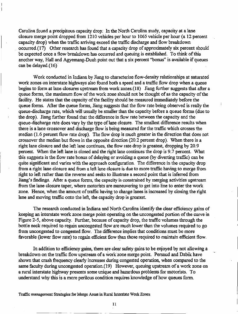
The size and growth of the queue is then dependent on the rate of arriving vehicles, the capacity of the bottleneck, and the relative density of the arrival stream and the vehicles in the queue. If the rate ofvehicles arriving is Ql and the capacity of the bottleneck is Q2, where the density of arriving vehicles is Kt and the density ofvehicles in the queue is K2, then Sin Equation 2-12 is the speed of the shockwave.(23) IfS is negative it means that the queue is growing and if it is positive it means that the queue is diminishing.

(2-12)

Figure 2-7 shows curves for the relationship between flow and density for the bottleneck (the merge point for the lane closure) and highway upstream. of the lane closure. The capacity of the upstream highway is Qc and the capacity of the bottleneck is Qb. If the flow rate upstream of the lane closure is greater than the bottleneck capacity (~), then the shockwave is moving upstream (backward moving) at the speed S. A backward moving shockwave is shown in Figure 2-7. Figure 2-8 shows a condition where the flow rate upstream of the bottleneck is less than the capacity of the bottleneck. In this case the queue is dissipating and there is a forward moving shockwave at speed S. ·

While collecting data in the field, the queue length was measured upstream from the work zone by a vehicle driving on the shoulder of the lane in the opposite direction. The data collection location of the vehicle and the queue is shown schematically in Figure 2-9. During times when the queue was experiencing spurts of growth, the driver of the data collecticm vehicle could not keep up with the growth of the queue and estimated that it was not uncommon, during very short. periods of time, for the queue to grow at speeds as high as 30 miles per hour. This illustrates one of the dramatic hazards ofbottlenecks along a rural freeway. Not only are vehicles approaching a work zone traveling at a high speed but the queue could be growing toward them at a rate of 3 0 miles per hour. In other words, a vehicle traveling at 65 miles per hour could in fact be closing with the upstream end of the queue at 95 miles per hour. The actual rate of closure (95 miles per hour) violates the driver's expected rate ofbraking and often causes high speed rear end crashes.

It is generally accepted that crash rates in work zones are higher than on highway section with similar traffic without work zones. For example, Pal and Sinha studied crash rates at freeway lane closures and found that there was a statistically significant increase in the crash rate in and around construction lane closures and that the increase was the greatest for lane closures where traffic crosses over the median and operates head-to-head on one side of the interstate.(24) In a recent study of crash rates in California interstate highway work zones, Khattak, Khattak,

and Council found that in the 36 sites examined, the rate of work zone crashes was 21.5 percent higher than it was before the locations became a work zone.(25)


14

_,;- Data Colection Vehicle. MOIIeS ..;th 1he ~am / end of 1he queue, reccrds position aver time.

rnm - ' --~----------------------------~~ml~~t~~Imr~mf.mti --------------------------

End of queue ToWorkZ~

Figure 2-9, Queue Length Data Collection Schematic

Understanding the safety hazard in the.queue itself(as opposed to other parts ofthe work zone) presents some difficulties. To understand the queue's impact on safety requires knowledge of the location of the crashes with respect to the location of the lane closure, the type of crash (rear-end, sideswipe, runriing into a fixed object, etc.), and the traffic operating condition at the time of the crash (free flow or queuing). Unfortunately, these data are not commonly available.

To collect these very data and to understand the role queuing plays in crashes in and around workzones, a research project was conducted by the Federal Highway Administration's (FHW A) Turner Fairbank Laboratory for the National Transportation Safety Board (NTSB).(26) NTSB was particularly interested in crashes 0 to .25 miles, 0.25 to 0.50 miles, and up to 4.0 miles upstream of the lane closure. ·

To satisfy the NTSB requirements, FHW A used two databases. One was supplied by the California Department of Transportation (CalTrans) and involved 28 freeway projects in California (17 were on freeways or expressways). The CalTrans database also included information on the location of the crash with respect to the location of the work zone. The second database was generated by FHW A from crash databases supplied by Minnesota and Dlinois. The Minnesota and Dlinois databases only provided information which indicated whether the crash occurred in the area of a work zone or at other locations along the freeway. The principle use for the Minnesota ~d Dlinois databases were to verify that the California data were indicative of crash rates in and in advance of work zones.

The California data are generally found to provide the same characteristics as the base data from the other two states and the author, therefore, concludes that the California data are indicative of work zone crash patterns elsewhere. Rear-end and sideswipe crashes are found to be more common at work zones than at other locations, accounting for more than 50 percent of crashes in work zones and only 38 percent at non-workzone locations. Rear-end crashes occur


16

Oensity(k)

Figure 2-7, Backward Forming Shockwave

a.

Density (k)

Figure 2-8, Forward Forming Shockwave


15

when individuals run into the car ahead in the queue and sideswipe crashes occur when an aggressive driver attempts to merge.

Based on the California data, rear -end crashes are occurring about three times as frequently as sideswipes, both in the work zone and upstream of the work zone. A review of national statistics also revealed that rear-end crashes result in a fatality or injury 33 percent of the time while sideswipe crashes result in a fatality or injury only 14 percent of the time, thus indicating that rear-end crashes are more hazardous. When the distance of the crash location upstream from the work zone is examined, it is found that rear-end crashes are more common as you move upstream. For example, the author found that "on a high-volume facility, rear-end accidents increase as the distance from the actual work activity increases." These results indicate that stopped vehicles in a queue are more lik~ly to suffer rear-end crashes than motorists elsewhere within the work zone. This finding implies that the possibility of become involved in a rear end crash is only exacerbated by backward-moving shockwaves.

ESTIMATING CAPACITY OF INTERSTATE LANE CLOSURES

Most highway agencies simply use the methods described in the Highway Capacity Manual to determine the capacity of a lane closure at an interstate work zone. The capacity estimates in the Highway Capacity Manual are based on the work done at the Texas Transportation Institute by a variety of investigators over a number of years throughout the late 1970s and the mid 1980s. This work is based on data collected on Texas Interstate highways by the Texas Transportation Institute (TTl) and done as part of"Study 292." Queue and User Cost Evaluation ofWork Zones (QUEWZ) is a software package used by many state transportation agencies to determine estimated delays, the length of queues, and user costs due to mergers at work zone lane closures. QUEWZ also originated from the same research program. Later (1987-1991), field data collection was conducted by TTl to update the capacity values and to revise and improve QUEWZ.(27) One of the more significant impacts of the updates was to change the factor for equating heavy trucks to passenger cars from 1.7 to 1.5. More recently, two studies have been done in North Carolina and in Indiana to try to determine the capacity of lane closures on interstate highways in those states.

Before investigating prior estimates of capacity, it should be recognized that not all estimates of capacity at lane closures are measured using the same criteria. The work done by TTl defined capacity as the hourly traffic volume under congested traffic conditions.(28) The TTl researchers identified capacity as full-hour volumes counted at lane closures with traffic queued upstream. They considered consecutive hours at the same location as independent studies. A Pennsylvania study defined the hourly traffic volume converted from the maximum recorded five minute flow rate as the work zone capacity. A California study measured volumes for three-minute time intervals during congested conditions. Two-three minute time intervals, separated by one minute, were then averaged and multiplied by 20 to determine the one-hour capacity values.(29) Dixon and Hummer define work zone capacity as the flow rate at which tratlic behavior quickly changes from uncongested conditions to queued conditions.(22) Jiang . defines capacity as the flow just before a sharp speed drop followed by a sustained period oflow


17

vehicle speeds and fluctuating traffic flow. It is Jiang's contention that what TTl was measuring was not capacity of the bottleneck but rather the queue discharge rate.(20)

TTl work zone capacity research published in 1982 was used as a basis for the methods for determining work zone capacity as described in the 1985 Highway Capacity Manual (as well as the 1994 manual).(27) This work was based on hour-long data collected on urban Texas freeways with lane closures. The applications of these data may be difficult to extrapolate to other locales due to the difference in driver behavior and differences in design of urban Texas interstate highway. Texas makes extensive use of frontage roads which makes it much easier for motorists to bypass congested segments of highway. The work conducted by TTl as part of Study 292 and work by other institutions and other individuals have resulted in a wealth of literature reporting on the measurement of queue discharge rates at work zones under a variety of factors which impact capacity. For example, one study investigated the sensitivity of capacities to the use of shoulders during lane closures and to splitting traffic when a center lane is closed.(30),(31) Some have looked at the type of traffic control devices and their placement and how they impact capacity and delay. Others have investigated pavement condition, night versus day, traffic volumes and traffic composition, merge discipline and speed control strategies, and the duration of work zones (short-term versus long-term).(31),(32),(33) Still others have investigated the relationship of the location of construction work to the traffic lane.(30),(34),(22)

The work Dixon and Hummer completed on capacities and delays at work zones conducted for the North Carolina Department of Transportation in 1996 probably provides the most sigriificant inference for Iowa. The North Carolina study included field data collected under conditions similar to those of interest to Iowa: lane closures on two-lane rural interstate highways. The North Carolina study used a more relevant measure of capacity for a lane closure than the TTl researcher: the traffic volume immediately before queuing begins. An important and unique finding of the North Carolina study is the identification of the location within work zone that governs the capacity. The location tends to vary with traffic conditions and with construction work activities .. The work done in Texas by TTl has assumed that the feature governing the capacity of a work zone lane closure is the point at the end of the taper. Dixon and Hummer report that the capacity of the work zone is governed by three locations. The capacity is controlled by the segment of the work zone travel path adjacent to the work area where the construction work activity is heavy; meaning large equipment and workers adjacent to the travel path. Under conditions where the work activity is low, then the capacity of the work zone (not the queue discharge) is governed by the end of the merge taper. However, even when the work activity is heavy, the capacity of the travel path adjacent to the work area was found to be about seven percent less than the capacity at the taper end for work zones on two-lane rural interstate highways. When a queue has formed, the work zone capacity is governed by the merging activity upstream from the work zone. In other words, once a queue has been formed, the capacity of the entire work zone is governed by the rate at which traffic can be discharged from the queue, which is generally at a lower rate than. the capacity of the taper end, accounting for the capacity drop.


18

What Do Other State Departments of Transportation Do?

To determine how other state departments of transportation (DOT) deal with congestion problems, we conducted telephone interviews of individuals representing 22 state DOTs during the summer of 1997. We explained the nature of our research and asked the representati~es if their agency was experimenting with innovative approaches to manage traffic through interstate work zones, if they have attempted to conduct any strategies to improve the capacity of interstate work zones, or ifthey have attempted to measure the capacity of interstate work zones. The responses we received are listed in Table 1.

North Carolina and Indiana currently are or have recently documented research on work zone capacity analysis, although other states believed that they have conducted research on work zone capacity but failed to document their findings. Texas conducted work zone capacity analysis and this research forms the basis for the methods described in the Highway Capacity Manual. Most states simply use the Highway Capacity Manual's methodology and their experience to evaluate traffic flow and delay in work zones.


19

I Table 2-1 Results of State Transportation Agency Interviews Agency and Contact Comments Arizona DOT No activity Mike Manthey, State Traffic Engineer California DOT Base capacity estimations on methods presented in the Highway Don F agel, Safety Capacity Manual. Research Colorado DOT Merging at lane closure approaches is a problem, especially in Mathew Reay, Traffic urban areas, but have not tried any new procedures to mitigate Engineer problems. Connecticut DOT Currently conducting some speed studies. Believed that they have Walter Coughlin, Traffic done some capacity analy~is in the past but nothing was published. Engineer Florida DOT Working on developing standards for ITS application but none JeffMorgan, Research have been for work zone related applications. No evaluation of Laboratory work zone traffic capacities. Georgia DOT No activity Marion Waters, State Traffic and Safety Engineer Indiana DOT (referred to Jiang has been collecting field data to measure capacities of work Purdue University) zones in Indiana and his findings have been reported in the Yi Jiang, Research literature.(20),(35),(36). Tarko was working on the field testing Assistant (now with the of a variable no pass zone. Indiana DOT) and Andrzej Tarko, Professor Kansas DOT Nothing has been conducted to date related to congestion at work Mike Crow, State Traffic zones but will be working with the other states in the region to Engineer evaluate new work zone traffic control technology. Michigan DOT Signing, particularly the location of changeable message signs and Bruce Monroe, Traffic arrow panels, has been investigated through their construction and Safety Division zone advisory committee. Another important issue in Michigan is

the reluctance of police to enforce work zone traffic control. No research has been initiated to manage work zone congestion.

Minnesota DOT Developed their own field manual for traffic control and have field Bill Servatius, Work Zone tested and deployed a work zone management traffic management Safety Unit field device (this is discussed in the technology section of this

literature review). However, no investigation has been conducted into capacity analysis of work zones.


20

Table 2-1 Continued A~ency and Contact Comments Missouri DOT Nothing has been conducted to date related to congestion at work Tom Borgmeyer, Traffic zones but will be working with the other states in the region to Engineer evaluate new work zone' traffic control technology. Nebraska DOR Working with the University ofNebraska to determine promising Dan Waddle, Traffic technology to better manage congestion in and around freeway Engineer work zone. Will also be evaluating work zone traffic control

technology with the other states in the region. New York DOT Experimenting with changeable message signs and planing to Thomas Werner, Traffic experiment with portable rumble strips. Have not evaluated work and Safety Division zone capacity or congestion management strategies. North Carolina DOT Experimenting with arrow boards and changeable message signs to Robert Cannalis, Traffic promote more orderly merge discipline, placement of rumble strips Engineer to promote attention to signs, and a variety of pavement markings. .

Conducted study with North Carolina State University to determine capacity ofwork zones.(21)

Ohio DOT Believed that there had been studies on work zone capacitie~ but Yuanita Elliot, Traffic nothing published. Currently negotiating a project with the Engineer University of Cincinnati to evaluate a technology which will inform

the driver the delay they should expect when traveling through an . interstate work zone.

Texas DOT Texas conducted a number of studies in the late 70s, 80s, and early Greg Brinkmeyer, Traffic 90s on work zone capacity analysis and this work has been the Engineering underpinning of most ofthe information available nationally. They

have done very little recently to incorporate innovative methods to control congestion in and around work zones.

Virginia DOT Nothing to report Dave Rousch, Traffic Engineer

INNOVATIVE WORK ZONE APPLICATIONS OF TECHNOLOGY

There is a wide variety of novel applications of technology to better manage traffic around and through work zones. Some focus on productivity improvements (delay reduction) and some focus on safety (e.g., reduction of speeds in work zones); however, to s0me degree, improvements in safety and improvements in productivity go hand in hand. In other words, applications with a focus on delay reductions improve traffic flow and, therefore, improve traffic safety.

Applications of technology can vary widely in scope. Some systems, like the Iowa DOT work zone web page, are statewide in scope and are focused on traveler information to allow individuals to make better route and/or travel time choices. Generally, these systems focus on a varjety of types of traveler information. For example, the Arizona DOT Trailmaster Highway

Traffic management Strategies for Merge Areas in Rural Interstate Work Zones 21

Closure and Restriction System (HCRS) provides information on all conditions which effect highway travel (e.g., incidents, weather, and congestion), not just roadway construction.(37) The HCRS involves an intranet system which carries information for use by the Arizona DOT to help support the management of its system. The system also acts as an extranet and carries information between the Arizona DOT and partner agencies (e.g., counties, state police, etc.), and an internet that provides information to the public. The intranet portion of the system only provides information on the location and type oflane restriction or closures for use by the public, while the other portions of the system, the extranet and intranet, are interactive and allow for two-way communication. The public can gain access to the public portion ofthe information system through the internet, through an automated telephone system, or through kiosks. Although the system provides useful information for the public, the agencies managing the highway system benefit greatly by having better information on current conditions and activities on the highway network. The Arizona DOT is working with adjacent states to expand the system to areas contiguous with Arizona. A similar system, the Condition Acquisition and Reporting System (CARS), is being developed by the Iowa DOT in conjunction with other states in the regton.

In urban areas, highway operating agencies will deploy traffic management systems to monitor traffic conditions; manage traffic through traveler information and traffic control devices such as ramp meters; and detect and manage incidents. To the extent that there are also work zones on highways under traffic management, they will also manage traffic in and around work zones. However, it is important to draw a distinction between urban highways under management

· and work zone locations. Typically, even if work zones involve urban construction, any surveillance, detection, and traveler information system must be in temporary locations (as opposed to permanent locations) due to the need to move field equipment as warranted by construction activities. For example, the Des Moines early deployment plan calls for surveillance and video detection cameras to be put in place along the I-235 right-way before the facilities reconstruction at temporary locations.(38) Later the same equipment could be permanently mounted adjacent to I-235 once reconstruction is completed. In rural work zones, where traffic volumes do not warrant permanent surveillance after construction, the ITS field devices (detectors, communication systems, changeable message signs, etc.) and any systems that are put in place during construction must be capable of being relocated.

Because of the costs involved, statewide or multistate traveler information systems, such as the public portion ofHCRS, operate with very little primary data and utilize data from secondary sources (police reports, reports from maintenance crew, reports from field offices, weather service information, etc.). These systems generally provide a variety of information in addition to work zone congestion and delay information for an entire state or multistate area. The primary intent of high level traveler information systems are to increase efficiency by allowing drivers to make more informed route and/or time of travel choices.

Some ITS applications, which provide work zone related user services, are more local and focus on the management of traffic in the area of the work zone. For example, during the summer of 1997, the Iowa DOT tested and deployed systems, including highway advisory radio (HAR), incident detection technology, changeable message signs (CMS), and video cameras, "to


. -----------------------------------------------------~

monitor approaching traffic speeds and volumes, determine when traffic backups occur, activate the warning devices, and inform surveillance personnel of the problem." (39) These systems manage traffic and incidents in the region of the work zone, focusing on the management of several aspects of the work zone but with a scope limited to a single work zone. Other systems, with features similar to the Iowa systems, have been tested over the last 5 to 6 years and are being deployed. A common attribute of all of these systems is that they operate in a reactive move. In other words, they wait for an incident or congestion to occur and then deploy management strategies to deal with the deteriorated condition. No systems were found that operate in a proactive mode where forecasts of traffic conditions (based on historical data or time series forecast of traffic volumes) and management strategies are deployed in advance to avoid or mitigate congestion.

Still other types ofiTS technology are limited to a single function. For example, the Ohio DOT has been field-testing equipment which informs drivers of the delay they can currently expect when traveling through a work zone upstream of their current location.(40) Once they are informed of the delay, the motorist can choose to divert to an alternative route or continue through the work zone. In limited field testing, the Ohio devices have received positive evaluations in motorist surveys. This type of device is intended to achieve a single mission. In the following sections, we briefly discuss technology being currently applied at the statewide and multistate level, at a multifunction level where traffic is managed in the region of the work zone, and at the single function level.

Regional, Statewide, and Multistate Systems

Traffic management systems and traveler information systems at the metropolitan and statewide level generally include information on work zones and develop management strategies to mitigate congestion caused by highway construction or maintenance. These systems, however, tend to have a much broader functionality than just informing travelers of maintenance or construction related lane restrictions. For Iowa, the issue of traveler information services on a statewide basis will be planned as part of the Iowa ITS Strategic Planning study currently being conducted (spring and summer, 1999). It is, however, important that the user services for informing motorists of work zones, likely work zone delays, and recommended diversion routes are accommodated in the statewide system architecture recommended by the ·consultant.

Although the current state ITS strategic plan will ultimately develop a system architecture for ITS services at the state level, it is important to recognize that travelers and commercial transportation services do not restrict themselves to political jurisdiction boundaries. An example of a group which has recognized that services must reach beyond state borders is the I-95 corridor coalition. The coalition is a group of 12 states stretching from Maine to Virginia along the eastern seaboard. The Information Exchange Network (lEN) created through the I-95 corridor coalition seeks to exchange information on traffic conditions, incidents, and planned. events which restrict highways in the corridor.(41) The network connects major transportation agencies in the corridor and the information is available for agencies to use and prepare for distribution to travelers. One creative use of the information available through lEN has been developed through an FHW A-sponsored (along with a whole myriad of private and public sector partners)


operational test titled TruckDesk.(42) The TruckDesk project demonstrated that information from lEN and other public and commercial information services could be processed and delivered to motor carrier dispatchers. This information adds enough value that motor carriers are willing to pay fees to support the service.(43) As a result, the project has moved to a self-supporting phase and changed its name to FleetForward. This project has been so popular that other travel information system projects (e.g., San Diego's Intermodal Transportation Management Center) are adapting similar services.(44) The value of these systems is proven by the private.sector's willingness to pay for information services.

Traffic Management Systems in the Region of the Work Zone

Generally, it is the objective of these systems to prove' an affordable means of delivering traffic management services, like the surveillance provided to an urban faculty under the management of a Traffic Operations Center (TOC). Typically, instrumenting a work zone with ITS field devices would not be financially feasible due to the cost of placing the highway under the management of a TOC. ·For example, the Minnesota DOT uses a figure of $500,000 as a planning number for placing a mile of interstate highway under the management of a TOC. Because of the expense, transportation agencies have focused on less expensive portable devices. A few mobile traffic management systems have been developed, tested, and are being used to manage the traffic in the area of work zones.

They typically involve video surveillance, traffic detection (using video detection or some other non-intrusive technology), and usually a combination of devices to communicate conditions to the drivers· and manage traffic, typically using changeable message signs (CMS) and/or highway. advisory radio (HAR). The Minnesota DOT's ITS office (Gudiestar), with a number of partners, has developed a field device they have titled the "Smart Work Zone" (SWZ).( 45) The SWZ is the second generation device. The first generation device was the Portable Traffic Management System (PTMS) and it was first field tested in 1994.(46) The objective ofPTMS and SWZ is to provide a traffic manager, located in a remote office, with video images and video detection in and around the work zone so that she/he can manage traffic through remote controlled CMSs. The · communication systems for the system are wireless due to the difficulty or impossibility of wireline communications in a work zone.

Portable work zone traffic management systems have proven beneficial. For example, the evaluation of swz found a significant increase in the traffic volume that traver~e urban freeway work zones while under the management of the SWZ. In the evaluation of SWZ a 3.6 percent increase traffic volumes in the morning peak were found and 6.6 percent increase in the afternoon peak. In addition, the system decreased the speed variability of vehicles approaching the work zone and decreased the average approach speed by 9 miles per hour. Other work zone traffic management systems have been·or are being developed elsewhere. For example, The Scientex Corporation has developed a commercially availablesystem called ADAPTJRTM_(47) Another system was developed by Computran Systems Corporation for the New York DOT.( 48)( 49) The Computran system is being developed for a large expressway interchange reconstruction ·project but has many of the same features as the SWZ.


Single Function ITS Work Zone Related Systems

There have been a number of attempts to develop systems which improve safety or the capacity of work zone lane mergers. Safety-related devices generally attempt to slow drivers approaching work zones through a number of strategies or protect the workers in the work zone through alarms, remote controlled shadow vehicles, automated flaggers, and decoy enforcement vehicles. In this review, we will focus on a few of these devices. Several more are being tested as part of the MidWest States Smart Work Zone Deployment Initiative and more equipment is being demonstrated and developed by highway agencies and technology vendors.

Efforts to Improve the Merger Discipline

As defined earlier in this literature review, the constraint imposed on the carrying capacity of a multi-lane highway due to a work zone lane closure varies with the level of activity in work zone and the condition of traffic flow through the lane closure. When the construction work adjacent to the travel lanes is heavy (construction workers and large equipment in close proximity to the travel lane), then the capacity is governed by the travel lane iinmediately adjacent to the active work area. Where construction is not heavy immediately adjacent to the travel lane, and prior to traffic volumes reaching saturation (prior to generation of a queue), capacity is governed by the end of the taper at the merge point. Following saturation, capacity is governed by merging activities upstream.ofthe merge point. Ifthe merger discipline of motorists can be modified to

. improve the efficiency of merger operations, then, after saturation has occurred, the work zone traffic throughput can be increased.

The failure of vehicles to merge into the through lane by the end of the queue can promote frustration on the part of some motorists. In an effort to avoid· waiting through a queue at a lane closure, some drivers will continue to travel in the closed lane, merging into the open lane as late as possible. This behavior can be a safety problem because late merging vehicles may take risks and accept unsafe gaps to merge. In addition, motorists who have already merged into the queue must watch in frustration as the late merging vehicles pass them. To block late merging vehicles, it is common to observe cars straddling both lanes or truck drivers who cooperate and travel slowly down both lanes side by side, thereby blocking cars proceeding down the closed lane. Both late merging and vehicles blocking the closed lane tend to reduce the capacity of the faculty at the merge point. As a result, the Pennsylvania and Indiana DOTs have attempted to modify driver behavior and improve merge discipline.

The Pennsylvania DOT's approach is to not encourage motorists to merge upstream from the lane closure and instead allow motorists to merge immediately upstream of the taper.(SO) Approximately 1.5 miles upstream of the merge point, a sign is posted stating "USE BOTH LANES TO MERGE POINT." At 350 feet upstream of the taper for the lane closure, a sign tells motorists to "MERGE HERE - TAKE YOUR TURN," thus allowing travel to the merge point in

)


·\.

the closed lane. By allowing travel in the closed lane, the tension between motorists merging early and late is minimized. ·

The Pennsylvania DOT's late merge program is a low technology approach to improving capacity. However, it was felt that it should be described in this section since other high technology approaches are being applied to enhance the capacity of the mergers on multi-lane facilities. They have studied the late merge approach and found that its application increased the capacity of merging operation by as much as 15 percent. (51)

The University ofNebraska-Lincoln (UNL) evaluated the late merge concept by testing its application at a Pennsylvania work zone.(50) The evaluation consisted of interviewing motorists and truck operators at a rest stop downstream of a work zone where the late merge concept had been applied. Although the late merge concept reduced the length of the queue by doubling highway capacity for vehicle storage (two lanes rather than one), many of the problems associated with merging traffic were simply pushed downstream to the merge point. Truck drivers, in particular, reported difficulties merging at the late merge point due to aggressive motorists. The authors of the UNL study interviewed only 88 motorists (58 automobile drivers and 30 truck operators) and, though they felt the findings were inconclusive, they did determine that the concept was not well received by drivers, especially truck drivers.

Another system with the objective of modifying driver merge discipline is the Indiana Lane Merge System (ILMS). A drawing of the concept is shown in Figure 2-10. The ILMS creates a variable no pass zone in the closed lane. In other words, immediately upstream from the merge taper are static signs which state, "DO NOT PASS," and one sign with fl~shing strobe lights (sign. I in Figure.2-IO) that states, "WORKSITE-DO NOT PASS WHEN FLASHING." Thus, the first four signs create a static no pass zone. The signs upstream are dynamic and the strobe lights on each activate when conditions warrant. On sign I (in Figure 2-1 0) a sensor is mounted which senses that the queue has reached sign I and activates sign 2. When the queue reaches sign 2, sign 3 is activated, and so on, thus creating a dynamic no pass zone.

The benefit of this approach is that signs create a no passing zone which starts before the end of the queue (assuming that the queue never exceeds the distance upstream of the location of the last dynamic sign). This should stop aggressive drivers who attempt to .bypass the queue by . traveling in the closed lane to the head of the queue. A prototype system was tested in Indiana in 1996 and more testing is to be conducted during the summer of 1999.(52) In simulation analysis conducted as part ofCTRE research (reported in the companion simulation report), a variable no pass system was evaluated using microscopic simulation. The CTRE simulation model results showed an increase in capacity and an increase in traffic speeds and reduction in delay when the variable no pass system is applied. However, unlike the actual application of this technology, our simulation model assumes all drivers will obey the signs.


DO NOT PASS Activation/

Z Board with , Deactivation

5 3 2 1

vehicle Dezector signal

~--·1----··" .4 ·-~···----....-·;;?.::" , .• ----~---··J.._ ______ ., I\ II H 1\ I I I \ I \ I I

I \ I I I \ I \ I I I \ I \ J I I

~ Traffu: ll ·~-------

J I I \

WORK ZONE

Figure 2-10, Conceptual Drawing oflndiana Lane Merge System (taken from (53))

Speed Reduction Technology

New technologies to reduce speed, speed variations, and the number and speed of high speed vehicles (above the 85th percentile) are still evolving. Several new technologies will be evaluated as part of the MidWest States Smart Work Zone Deployment Initiative during the summer of 1999 (a project in which the Iowa, Kansas, and Missouri DOTS and the Nebraska Department of Roads are participating). However, here we examine only two existing speed reduction technologies which have had significant evaluation and testing.

One technology Is the use of a drone radar device to make drivers with radar detectors believe there are radar-equipped enforcement personnel in the vicinity of the work zone. This has the effect of slowing down drivers fearful of being cited for speeding. Several evaluations have been conducted of this type of device and it has been shown to reduce the average speed and reduce the percentage of high speed vehicles. A study of unmanned radar by Pigman et al. at high. crash frequency locations along I-75 in Kentucky found that at one of the two experiment sites, the average speed was reduced by 1.7 miles per hour.(54) Also, the variance of speeds and the 85th percentile speeds were reduced at both locations. Ullman and Riesland conducted an evaluation of unmanned radar by observing speeds immediately upstream from work zones with drone radar units at eight sites in Texas.( 55) At the seven sites where large speed data sets were collected, the deployment of the drone radar reduced average speeds from 0.2 miles per hour to 1.7 miles per hour. At some of the sites, a greater speed reduction was noted for trucks as compared to cars and a greater reduction was noted in the speed of high speed vehicles as compared to the average speed of all vehicles. · ·


In Illinois, Benekohal, et al. evaluated unmanned radar in a work zone for a few hours. They found that within the first few minutes of radar operation, the average speed reduced by almost 10 miles per hour. However, over a three hour data-collection period, there was not a statistically significant reduction in average speed.

A Virginia study of unmanned radar by Turochy and Sivanandan evaluated the system at three work zones, each with a different configuration.(56) Two were long-tenn work zones (multi-day construction projects) while the third project was a short-term project, lasting only one day. In all three cases, a reduction in average speed was observed although in one case it was not statistically significant. The average speed reduction observed ranged from 0.8 miles per hour to 2.3 miles per hour. The researchers also observed reductions in the standard deviation ofspeed of 0.1 miles per hour to 0.5 miles per hour, a reduction in the traffic exceeding the speed limit by 6 to 20 percent, and a reduction in the 85th percentile speed of 1.1. miles per hour to 3. 9 miles per hour. The authors conclude that unmanned radar is more effective in temporary work zones, presumably because in temporary work zones drivers do not get enough exposure to the operation to know that there are no enforcement personnel present in the work zone. They also conclude that in work zones where motorists have the expectation that enforcement officials may be present, the unmanned radar can be just as effective at reducing speed as having an enforcement personnel present.

Another technology used to reduce speed is the radar speed monitor display. This is a device which automatically monitors and displays .the speed of vehicles passing through the work zon~ using radar. The objective is to make drivers aware of their speed through digital display and drivers with radar detectors are likely to believe that their speed is being monitored by enforcement personnel. The Iowa DOT deployed this technology in the mid 1970s when it mounted a speed monitor and display device over I-35 just south or Ames, Iowa in the south bound lane. Similar devices were used for traffic calming iri Berkeley, California, where they reduced average traffic speed by as much as 20 miles per hour.( 57)

McCoy, et al. evaluated the speed monitor display device for the South Dakota DOT in 1993. When placed in advance of work zones, these devices were found to be effective and reduced average speeds by four to five miles per hour. In addition, the number of high speed vehicles was reduced. They found that the number of vehicles exceeding the advisory speed by more than 10 miles per hour was reduced by 40 percent. McCoy, et al. concludes that the speed . display system appears to have more beneficial impact than unmanned radar.

CHAPTER CONCLUSIONS

This chapter first presented fundamental principals oftraffic flow theory.to provide readers with a foundation to assist them in understanding the context of research related to the capacity of work zone lane closures. Much information on the capacity of work zone lane closures and delays was developed through research conducted by the Texas Transportation Institute (TTI) through a seri~s of projects which started in the late 1970s·and continued through the 1980s. The results of the TTI work are commonly used by transportation agencies and the findings are the basis of the lane closure capacity analysis reported in the Highway Capacity


Manual. Only recently has significant additional research been conducted in other locations (other states) to add to the body of knowledge on work zone lane closure capacity. One of the more important additions to recent research was to provide a clearer definition of the capacity of work zone lane closures.

The TTl work defined traffic carrying capacity of a work zone lane closure to be traffic flowing through the work zone under congested conditions. Jaing points out that the volume under congested conditions is really the queue discharge traffic flow rate and not the capacity of the lane closure. (3 5) In most cases, the peak flow immediately before saturation is really greater than the flow through the system after saturation. Therefore, Jaing defines capacity as the volume of traffic flowing through work zones immediately before congestion generates a queue.

The phenomenon where both average speed and volume drop after saturation is known as capacity drop. Because of capacity drop, the traffic volumes through the bottle neck required to regain uncongested flow are much lower than the volumes required to go from uncongested to congested flow. The difference implies that conditions must be more favorable to regain efficient flow that those required to maintain efficient flow. Thus there is a capacity bonus for keeping traffic flows below the level where the lane closure becomes saturated.

Our review of work zone-related ITS technology found that ITS applications dealing with work zone traffic management and traveler information focus at three levels. At the highest level, there is traveler information that operates on a region, statewide, or multi-state level. Although providing travelers with information regarding possible delays due to work zones is an important feature, these systems typically report information for all types of road closures and restrictions (e.g., restrictions caused by weather or an incident). The next level down are mobile systems that attempt to manage traffic in the area of the work zone. These utilize a number of field devices (e.g., CMSs, HAR, video surveillance, etc.) in combination with managing traffic. The last level are applications with a single purpose, e.g., reduce the speed of traffic through the work zone, inform drivers of the travel time through the work zone, or improve traffic flow by modifying the merger discipline. Systems at all three levels tend to be reactive rather than proactive. Others wait for congestion to build, then assist traffic managers to better manage the congestion that has already occurred. It appears that there is a great deal of opportunity to develop systems which are proactive and implement strategies in advance of congestion. For example, a system which is capable of predicting when congestion is likely to occur could be used to deploy diversion strategies well in advance and upstream of the lane closure, possibly delaying or avoiding saturating the lane closure.


CHAPTER 3: SITE SELECTION

CTRE project team personnel met on two occasions with Iowa DOT staff to identify attractive data collection sites. During the meetings, which were held on April28 and May 15, 1998, a list of essential criteria for an acceptable data collection site was developed and potential work zone locations were identified.

CRITERIA FOR A SUITABLE LOCATION

The April 28 meeting included Iowa DOT staff members Mark Bortle, Steve Gent, Dan Houston, Dan Sprengler and CTRE's Dennis Kroeger and Steve Schrock. The objective of the meeting was to determine suitable criteria for an acceptable data collection site. ,.

The DOT staff determined that an ideal location would be a section of interstate where work zone congestion had occurred in previous years. In general, this included Interstate 80 from Des Moines to Davenport, Interstate 3 5 from Ames to Des Moines, and Interstate 3 80 from Iowa City to Cedar Rapids. It was also decided to keep the sites rural if possible to reduce the impact urban commuters have on speed and headways. Urban locations would be used, however, if no other suitable locations could be found. '

The types of projects that might provide a suitable merge area at which to collect data were discussed. The Iowa DOT staff believed that a long-term construction project would be advantageous because it would provide the duration needed to collect multiple days of data. It was also decided to try to use shqrter-term construction or maintenance projects if they took place within the areas discussed above, but only as an alternative to long-term work zones. Any project where the work zone layout would be static for at least one day would be adequate for the purposes of data collection.

The desired physical attributes of the interstate at a possible data collection site were also discussed. Ideally, locations that were as far as possible from interchanges were desired in order to minimize the impacts of merging traffic. Also, in order to keep all potential locations roughly equal, it was decided to only look at merge areas where two lanes of traffic were reduced. to one. This would eliminate many projects on urbanized sections of highway, and also where on-ramps or acceleration lanes were present. A summary of the criteria from this meeting is provided in Table 3-1.

Iowa State University (ISU) graduate and undergraduate students were schedule to perform the field data collection. Due to university schedules a data collection window existed from the end of spring classes to the beginning offall classes. This allowed fifteen weeks from. May 11, 1998 to August 21, 1998 to collect data. Any construction or maintenance project that was not scheduled for this time period would not be included in.the project.


Table 3-1 Criteria for a Suitable Data Collection Site Category

High Traffic Locations

Duration

Urban vs. Rural

Time Frame

Physical Attributes

SELECTION OF SITE CRITERIA

Desirable Locations/Attributes

• I-80 from Des Moines to Davenport.

• I-35 from Des Moines to Ames.

• I-380 from Iowa City to Cedar Rapids.

• Long-term work zone preferred: Short-term closures acceptable.

• Rural preferred. Urban acceptable as a secondary alternative.

• May 11 to August 21, 1998 .

• Far from interchange location.

• Two lanes of traffic reduced to one.

A list of all construction and maintenance projects that were to take place on Iowa's interstates was developed by the Iowa DOT's construction office. This list represented all planned work on the interstate system considered to be possible locations, and is shown in Table 3-2. The CTRE project team narrowed this list through telephone conversations with Iowa DOT engineers and field inspectors familiar with each project. All projects that were not located on Interstates 80, 35, or 380 were eliminated, based on the assumption that enough volume would not be present to create congestion. Any projects that were not planned to take place from May 11 to August 21, 1998 were eliminated. The reasons individual projects were eliminated as potential data collection sites are provided in Table 3-3. Communication with the Iowa DOT Transportation Centers continued throughout the summer. These Transportation Centers provided information about updated start dates for projects that had not yet started but were planned to start during the data collection window.

This process reduced the list to only five viable sites, which are shown in Table 4-4. This shortened list was presented to the Iowa DOT on May 15, 1998. Two of these projects, I-35/80 at Merle Hay Road and 1-74 from the Mississippi River to I-80, were in urban locations, and were considered secondary. Additionally, the project at Merle Hay Road would only have traffic control in place at night, which further reduced the attractiveness of the location. However, it was believed that congestion could still occur, so it remained on the list of potential site's.

The illinois and Minnesota DOTS were contacted to determine if any acceptable collection sites could be found in those states to increase the number of suitable locations. It was believed that these states could provide traffic situations similar to those found in Iowa, and that the data would be comparable. The Minnesota DOT did not anticipate congestion at any of their planned work areas during 1998, so it did not recommend that the project team come to Minnesota. The illinois DOT, however, agreed to allow data collection on Interstate 80 at a work

Traffic management Strategies for Merge Areas in Rural Interstate Work Zones ' 32

zone stretching from the Mississippi River to the Rock River. This site appeared to be acceptable~ and some congestion was expected by Illinois DOT officials.

SUMMARY

By mid-May, the only work site on the list of suitable collection sites actually under; construction was on 1-80 from US 61 to 1-74 by Davenport. This site was therefore selected as the primary location for data .collection. Although the project team expected to focus on other locations later in the summer, this location remained the primary data collection site for the entire summer. The Davenport location was visited on 19 days when congestion was anticipated. It was also the only location where congestion was actually observed.

At the May 15 meeting, the Iowa DOT staff also reviewed the proposed field data collect~on procedure to determine if additional safety procedures were needed, and to provide advice for increased efficiency in data collection. The procedure that was adopted is detailed in the following chapter.


Table3-2 1998 Merge Area Stud:f: Candidate Projects Route Project Number ADT County Location and Activity

1-29 IMN-29-3(56)54--0E-78 63,000 Pottawattamie West 1-80 interchange to lA 192 interchange, NB & SB[PCC Patching)

1-29 IMN-29-4(56)72--0E-43 38,100 Harrison Pottawattamie Co. line to South Dakota State line[PCC Patching]

1-35 IMN-352(258)66-0E-77 27,500 Polk Warren County line to West Mixmaster, NB & SB[PCC Patching)

1-35 IM-35-3(71)81--13-77 55,100 Polk Merle Hay Road interchange, EB & WB[PCC Reconstruction]

1-35 IMX-35-3(96)88--02-77 56,000 Polk Northeast Mixmaster (1-35/80/235 interchange)[Guardrail and Bridge

Retrofits]

1-35 IMN-35-5(77) 111-0E-85 20,000 Story M.P. 106 to County Road C-47 in Franklin County[PCC Patching]

1-74 IMN-74-1(113)0--0E-82 60,100 Scott Mississippi River Bridge to 1-80 interchange[PCC Patching]

I-80 IMN-80-1 (234 )2--0E-78 52,700 Pottawattamie Nebraska State Line to lA 224 interchange, NB & SB[PCCPatching]

1-80 IM-80-1(235)23--13-78 16,500 Pottawattamie lA 224 interchange to 1-680 interchange, WB[PCC Reconstruction]

1-80 IMN-80-5(211) 141--0E-77 52,100 Polk 1-80 at the US 65 interchange, EB & WB[PCC Patching]

1-80 IMN-80-5(199) 174--0E-79 32,700 Jasper lA 224 interchange to east of US 63 interchange, EB & WB[PCC

Patching]

1-80 IMN-80-6(206)240--0E-52 44,500 Johnson I-380 interchange to Iowa 1 interchange, EB & WB[PCC Patching]

1-80 IM-80-6( 170)243--13-52 39,000 Johnson Iowa River Bridge in Iowa City, EB & WB[Bridge Widening]

1-80 IM-80-6(174 )243--13-52 39,000 Johnson Iowa River Bridge in Iowa City, EB & WB[PCC Median Paving]

1-80 IM-80-8(171)295--13-82 32,600 Scott US 61 interchange to 1-74 interchange, EB & WB[PCC

Reconstruction]

1-80 IMN-80-8(182)295--0E-82 20,600 Scott Middle Road interchange to Mississippi R. Bridge, EB & WB[PCC

Patching]

1-235 IMN-235-2(251)73--0E-77 103,800 Polk _ West System interchange to the East System Inter:change [PCC

Patching]

1-280 IMN-280-1(113)0--0E-82 22,900 Scott Mississippi River Bridge to 1-80 interchange, NB & SB[PCC Patching]

1-380 IMN-380-6(204)243--0E-05 75,800 Johnson From 1-80 to US 218 in Waterloo, NB & SB[PCC Patching]


Table 3-3 Reasons for Elimination of Potential Data Collection Sites Project Number

IMN-29-3(56)54-0E-78

IMN-29-4(56)72-0E-43

IMN-352(258)66-0E-77

IMX-35-3(96)88--02-77

IMN-35-5(77)111-0E-85

IMN-80-1(234 )2-0E-78

IM-80-1(235)23-13-78

IMN-80-5(211)141-0E-77

IMN-80-5(199)174-0E-79

IMN-80-6(206)240-0E-52

IM-80-6(170)243-13-52

IM-80-6(174)243-13-52

IMN-80-8(182)295-0E-82

IMN-235-2(251)73--0E-77

IMN-280-1(113)0-0E-82

Project Number IM-35-3(71)81-13-77

IMN-35-5(77)111-0E-85

IMN-74-1(113)0-0E-82

IM-80-8(171)295-13-82

IMN-380-6(204)243-0E-05

lllinois DOT Project

Reason For Elimination

Did not have sufficient volume to create congestion



Traffic control scheduled only for nighttime




Not scheduled until Fall1998

Not scheduled until Fall 1998

2 lanes of traffic through work site in each direction, no merge



Between two other work zones (IM-80-8(171)295-13-82 and the

lllinois DOT construction project)

Traffic control scheduled only for nighttime


Table 3-4 Suitable Data Collection Sites Location Work Activity . Estimated Time

Merle Hay Road PCC Reconstruction Summer and Fall interchange 1998 Interstate 35 from Des Milepost 106 to C-47 in Summer 1998 Moines to the Franklin County Minnesota border Mississippi River PCC Patching Summer 1998 Bridge to I-80 US 61 interchange to PCC Reconstruction April - September I-74 interchange 1998 1-80 to US 218 in PCC Patching Summer 1998 Waterloo, NB & SB 1-80 from the PCC P,atching and Summer and Fall Mississippi River to the ACCOverlay 1998 Rock River

Traffic management Strategies for Merge Areas in Rural Interstate Work Zones . 35

CHAPTER 4: MOBILE TRAFFIC DATA COLLECTION OPERATIONS

This chapter examines the field equipment and methodology used for this project and provides a basic overview. Details ofthe laboratory analysis can be found in Chapter 5.

The equipment was purchased jointly by the Iowa DOT and CTRE. The assembly of the individual component parts into the completed data collection trailers was accomplished by Iowa DOT staff

EQUIPMENT

The mobile field data collection trailers were designed to collect video images of interstate traffic at specific locations, such as work zone merge areas. The equipment was designed to be positioned near the traffic lanes in the median or on the shoulder. Each trailer was designed to raise two surveillance cameras to a height of about 30 feet above the highway using a hydraulic mast. The video images are recorded onto Super-VHS (SVHS) videotape for later laboratory analysis.

The component parts for two field data collection trailers were purchased through ISU's Central Stores. A list of the components for the trailers, including a description of how each component was used in the completed system, is provided in Table 4-1 . Pictures of one of the data collection trailers and its electrical components can be seen in Figures 4-1 and 4-2.

Table 4-1 Field Data Collection Trailer Component Parts Component Parts for each Trailer

Interstate Manufacturing IF-46SAFS Cargo Trailer Autoscope AS-CAM Surveillance Camera (2) Vicon V113APT-1 Panffilt Unit (2) WilBurt Telescoping Mast System Model No.

7-30-357/367 Burst Electronics TC-3 Time Code generator (2) Panasonic PV-S6490 Super-VHS VCR (2)

Kramer VM-41 Passive Video Switcher

Panasonic TR-990C 9" Video Monitor Honda EX-1000 Portable Generator

Use Mobile trailer platform Video surveillance Allows for camera movement Elevates the Autoscope cameras to an approximate height of 30 feet above the highway Time-stamps the video images Records video images for laboratory analysis Allows viewing of multiple video feeds through one monitor Allows viewing of camera output in the field Provides electricity to the system


-------------

Figure 4-1 Field Data Collection Trailer in Operation

FIELD DATA COLLECTION METHODOLOGY

The intent of this project was to determine traffic characteristics at the merge area of an interstate work zone. In order to collect data at such a location, it was necessary to determine the optimal placement of the field data collection trailers. The ideal location would allow adequate viewing of the highway with all four cameras, while maintaining the highest standards of safety, both for the driving public and the data collection team.

Traffic Video Collection

After discussions with Iowa DOT staff and a review of a set of plans for a standard Iowa DOT merge area, locations to position the trailers were selected. An example of a trailer set up behind a roadside barricade can be seen in Figure 4-1 . The layout of a standard work zone merge area, including the placement of the data collection trailers, is shown in Figure 4-3 .


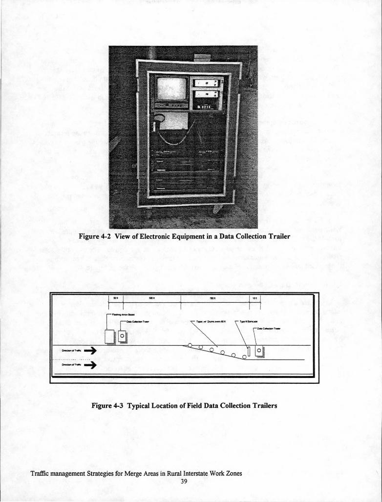
Figure 4-2 View of Electronic Equipment in a Data Collection Trailer

J ... j "'' J '"" J ... J

r r r r

~---~OD~T,....

~~--Q[j Clftc:loltf/I T~~

....... .... . .. . -

~fiiT...-e~

Figure 4-3 Typical Location of Field Data Collection Trailers


This layout provided increased safety for the project team by allowing the setup and operation of the data collection trailers while staying behind existing equipment and barricades. These locations also made the trailers less conspicuous to motorists, as the trailers were at least partially shielded from view. This basic layout was used throughout the data collection phase with little variation. Note that in Figure 4-3, the left lane is closed. In situations where the right lane is closed the locations of the flashing arrow board, drums, barricade, and trailers would be placed on the right-hand side of the highway rather than the left.

Once the equipment was in position, the traffic was recorded on videotape. One camera on each trailer was positioned to record traffic just upstream from the trailer, with the second camera in each pair looking downstream. The layout described above allows the trailers to collect video images of vehicles as they passed the flashing arrow board and as they passed the end of the taper in the transition area.

Once the trailers were in place and operating, a calibration grid was painted on the shoulders of the highway within the field of view of each camera. This grid was required to use the Autoscope Supervisor software during the laboratory analysis to accurately determine the speeds and lengths of the vehicles.

The marks for the grid were placed on the highway shoulders. Each mark was made with white paint and in the shape of rectangles measuring 8" by 16". The distances and angles between each of the marks were accurately measured using a total station. This surveying tool allowed distance accuracy ofO.l ft and angle accuracy of 10 seconds of one degree. The use of the total station allowed accurate measurements without requiring the personnel or the equipment to be in the traveled lanes. An example of a completed calibration grid is shown in Figure 4-4.

Queue Length Data Collection

When a queue developed, the project team would move to the outside shoulder of the interstate, adjacent to the opposite direction of traffic. From this location, a project team member in a vehicle followed the upstream end of the queue without causing additional disturbances to the queued traffic. The data collection team was able to safely follow and record the queue length over time, using the milepost markings on the reflectorized delineator posts in the ditch to record the location of the end of the queue. This information was a necessary component in determining an estimate of the number of vehicles in the queue, which was used later to determine the total delay cost of the observed queues. An example of this process can be found in Figure 4-5 .


I I

Flashing Arrow Board

,/···_,···

/

.· ,..··

- ··- ·-- -·- ··-- ·- ·- ··-··- ---··- -- -·--·-- -·-- ·- ···-·-···- - - -·?-·-- ···- ···- -

I I I / ...... /

,.····· _,. ... ,.··

.. ··

/ ..

... .. ··"'"

.t' ....

Figure 4-4 Typical Placement of a Calibration Grid

Figure 4-5 Example of Collection of Queue-Length Data

RESULTS OF SUMMER DATA COLLECTION

Traffic backups were observed on Interstate 80 at Davenport on June 19, July 2, July 10, and August 7, 1998. Traffic volumes rose high enough that not all vehicles could be accommodated at their desired speed. Congestion and delays resulted, and were recorded by the project team.

The other main site where data were collected was on Interstate 80 at the Rock River Bridge in lllinois. However, no usable data were collected here, as traffic levels never approached capacity during the site visit. Other potential sites were not visited for various reasons. The sites near Des Moines were excluded because the work was performed at night. The maintenance work that was performed on Interstate 380 between Cedar Rapids and Iowa City was switched to night work by the Iowa DOT to prevent congestion, which eliminated it as a usable site for our needs. The maintenance project on Interstate 35 north ofDes Moines and the maintenance project on Interstate 74 in urban Davenport did not start until after the end of the summer. Table 4-2 shows the dates and locations of the field data collection.

Date 5/27/98 5/28/98 5/29/98 6/19/98

Table 4-2 Summary of Data Collection Dates and Locations Data Collection Location

IM-80-8( 171 )295-13-82, Interstate 80 near Davenport IM-80-8( 171 )295-13-82, Interstate 80 near Davenport IM -80-8( 171 )295-13-82, Interstate 80 near Davenport IM-80-8( 171 )295-13-82, Interstate 80 near Davenport


6/26/98 6/30/98 7/1/98 7/2/98 7/3/98 7/9/98

7/10/98 7/17/98 7/26/98 7/29/98 7/30/98 7/31/98 817/98

8/14/98 8/21198

IM-80-8(171)295-13-82, Interstate 80 near Davenport IM-80-8(171)295--13-82, Interstate 80 near Davenport IM-80-8(171)295--13-82, Interstate 80 near Davenport IM-80-8(171)295--13-82, Interstate 80 near Davenport IM-80-8(171)295-13-82, Interstate 80 near Davenport IM-80-8(171)295-13-82, Interstate 80 near Davenport IM-80-8(171)295-13-82, Interstate 80 near Davenport IM-80-8(171 )295-13-82, Interstate 80 near Davenport

Interstate 80 at the Rock River Bridge, Illinois Interstate 80 at the Rock River Bridge, Illinois Interstate 80 at the Rock River Bridge, Illinois Interstate 80 at the Rock River Bridge, Illinois

IM-80-8(171)295-13-82, Interstate 80 near Davenport IM-80-8(171)295-13-82, Interstate 80 near Davenport IM-80-8(171)295--13-82, Interstate 80 near Davenport

Limitations of Data Collection at the Davenport Location

The capacity of the merge areas was reached on only four occasions while the project team was on site. There are several possible reasons why more backups were not observed. One reason is that the work zone was only four miles east of the Interstate 80/280 system interchange. Signs warning of several work zones on Interstate 80 were placed at the interchange, encouraging the use oflnterstate 280 as an alternate route for eastbound traffic to bypass the work zones. This bypass possibly reduced volumes on Interstate 80 at the work zone enough to prevent some backups.

The work zone merge area for the westbound traffic was placed just downstream from an onramp with an acceleration lane adjacent to the traveled lanes. This resulted in giving the interstate a three-lane configuration at the point of the merge. In order to minimize the variations in the geometry, the study was confined to the merge area for the eastbound traffic at this work zone.


N

I

Figure 4-6 Location of the Data Collection Site at Davenport

SUMMARY

This methodology allowed the project team to collect video data of vehicles as they passed the flashing arrow board and the end of the merge taper of an interstate work zone. These video images were analyzed using the Autoscope 2004 Machine Vision Processor to convert the video into vehicle characteristics, such as vehicle speed, length, and lane choice. This process will be explained in Chapter 6.


CHAPTER 5 LABORATORY DATA REDUCTION

The SVHS tapes with traffic recordings were brought back to the laboratory and analyzed by the Autoscope 2004 Wide Area Vehicle Detection System. Traffic characteristics of each vehicle were recorded and saved as text files using the Autoscope, and then imported into spreadsheet format for further analysis.

AUTOSCOPE DATA REDUCTION

The Autoscope detects changes in the visual images it receives to determine vehicle characteristics such as speed and length. It also is able to determine the characteristics of the entire traffic stream, such as the total number of vehicles that it detects in a given time period. The Autoscope uses a technology called machine vision processing to determine these changes. A simple explanation of machine vision processing is that the Autoscope looks for color changes in each pixel on the screen image. Determining when and how fast these pixels change color is how the Autoscope determines a vehicle's characteristics.

In order to get accurate readings from the Autoscope, the system was calibrated using the calibration feature in the Autoscope Supervisor software. Using the painted grid marks explained in the previous chapter, an accurate calibration grid was drawn. The software requires that at least five virtual lines be placed over the top of the screen image in the shape of a grid. This grid is formed with lines running both parallel and perpendicular to the direction of traffic flow. The height of the camera above the highway is also required to complete the calibration. This provides the Autoscope with enough information to determine the plane in which traffic is traveling. An example of this setup is shown in Figure 5-l . With this, the Autoscope can observe images on the videotape and determine the speed and length of each vehicle.

Using the Supervisor software, virtual detectors were placed over the image of the traffic lanes. These detectors were then used to determine each vehicle's speed, length, and classification, much like loop detectors would if placed at that location. The proper placement of these detectors provides the lane distribution for the traffic at the flashing arrow board. Determining the lane distribution was not necessary for the video taken at the end of the merge area because traffic had merged into one lane by that point. Figure 5-2 shows an example of two virtual detectors placed over the highway near the flashing arrow board upstream from the merge area.

Once the virtual detectors were designed for each camera view, the detector files were downloaded into the Autoscope. With these files in place, the Autoscope could analyze the videotapes and record the traffic characteristics. The Autoscope is capable of reading data from two video feeds at one time. The data collected in this manner was then downloaded into the hard drive of the laboratory desktop computer for further analysis.


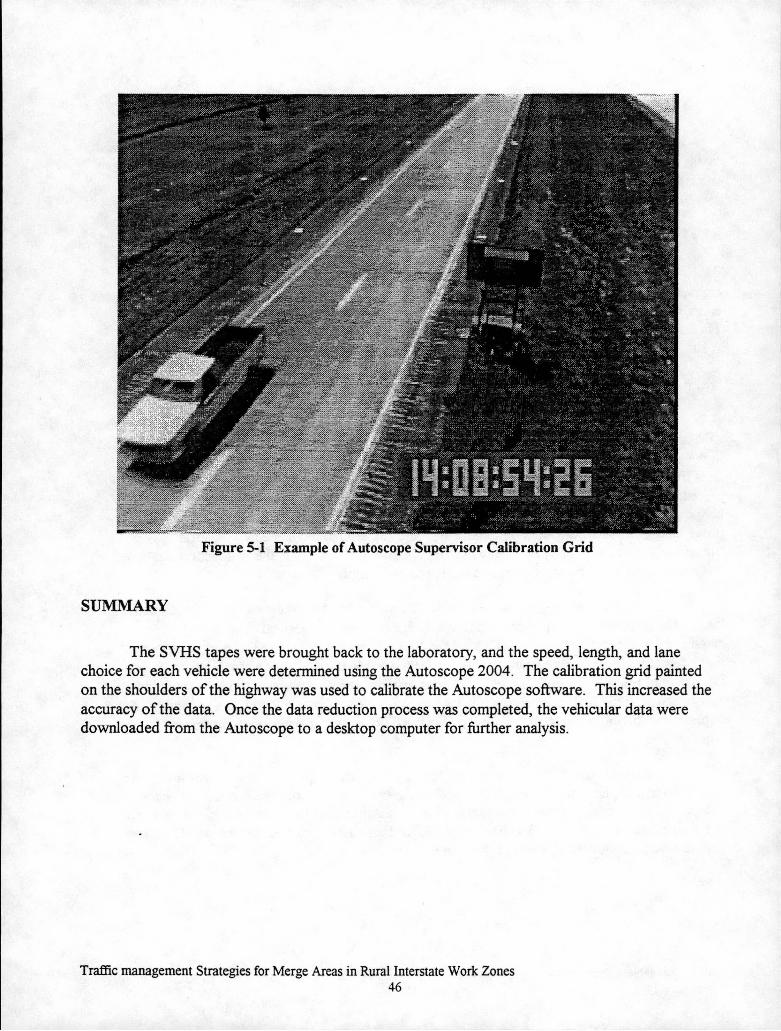
Figure 5-l Example of Autoscope Supervisor Calibration Grid

SUMMARY

The SVHS tapes were brought back to the laboratory, and the speed, length, and lane choice for each vehicle were determined using the Autoscope 2004. The calibration grid painted on the shoulders of the highway was used to calibrate the Autoscope software. This increased the accuracy of the data. Once the data reduction process was completed, the vehicular data were downloaded from the Autoscope to a desktop computer for further analysis.


Figure 5-2 Example of Virtual Detectors Placed over Video Image


CHAPTER 6: ANALYSIS AND RESULTS

This chapter details the analysis of the traffic data from the Davenport work zone. The results obtained include an improved estimate of the capacity of a standard Iowa DOT work zone merge area, queue data including the lengths of the observed queues, how the upstream end of these· queues behaved, and an estimate of the user cost incurred by motorists in these queues. This chapter ends with some recommendations about how this information can be used to improve the planning process for future htterstate work zones.

CAPACITY

· Traffic backups were observed on Interstate 80 at Davenport on June 19, July 2, July 10, and August 7, 1998. Data for these dates were analyzed to determme how traffic operated during

. congestion:

Determining Capacity

The traffic flow data that were collected for the four days and the corresponding vehicle classification percentages are shown in Tables 6-1 and 6-2 to illustrate the type and amount of traffic observed. The units for Table 6-1 are in vehicles per hour.

Table 6-1 Observed Unconverted Traffic Volumes By Lane

Date Time Total Left Right

Can Trucks Cars Trucks Can Trucks 6/19/98 1-7pm 5,518 1,494 190 81 5,328 1,413 7/2/98 9 am-9pm 10,636 2,439 638 371 9,998 2,068

7/10/98 8am-6pm 8,421 2,030 8,392 2,006 29 24 817/98 2-:-7pm 4,751 1,581 4,691 1,529 60 .52

Table 6-2 Observed Unconverted Traffic Percentages %By Lane

Date Time Total% Trucks

Left Right Can Trucks Can Trucks

6/19/98 1-7pm 21.3% 70.1% 29.9% 79.0% 21.0% 7/2/98 9am-9pm 18.7% 63.2%. 36.8% 82.9% 17.1%

7/10/98 8 am-6pm 19.4% 80.7% 19.3% 54.7% 45.2% 817/98 2-7prri. 25.0% 75.4% 24.6% 53.6% 46.4%

·Traffic volumes are converted to passenger car equivalents froin the observed data collected with the field equipment. Trucks are converted to 1. 5 passenger cars, which is taken from the 1994 Highway Capacity Manual for trucks on a level grade.( 58) These converted data


were then analyzed in five-minute increments to determine the traffic volume in passenger car equivalents.

The capacity of a work zone is really the highest volume observed immediately before the flow breaks down and queuing begins. Once queuing begins, the traffic volume passing thfough the work zone is really a measure of the queue discharge rate. Therefore, the highest volumes immediately before a queue occurs are considered to be indicative of a work zone's capaCity and these values are measured. This measure of capacity was defined by Jiang. Jiang found that the highest sustained free flow volumes through a work zone tend to occur just prior to a sharp speed drop.(59)

On July 2 and July 10, 1998, data were collected continuously from early morning until evening. The data gathered during the time a queue was present were temporarily set aside in

1 order to examine only the free flow data. The ten highest converted free flow values were identified for each day. These data were studied to determine a pattern to the peak free flow values. As shown in Figure 6..: 1, when averaged over five-minute time increments, eight of the ten highest free flow values on July 2 occurred within 1 hour and 45 nlinutes prior to the beginning of the queue. On July 10, seven of the ten highest free flow values occurred within 90 minutes of the breakdown and the beginning of the backup, as shown in Figure 6-2. The majority of the highest free flow volumes occurred within two hours of the breakdowns on both days. The averages of the ten highest observed free flow values were calculated as an approximation of the threshold volumes at which a breakdown could be expected: · · ·

The breakdowns on June 19 and August 7 were not analyzed in this manner because data on these days were only collected for approximately two hours prior to queue development. This shorter range of time values did not allow for accurate comparisons of the highest free flow values against data for the entire day. These traffic flows just prior to the onset of the major speed drop and the beginning of queued conditions on these days were comparable, however, to the July 2 and July 10 data. The graphs of the traffic flows and speeds for June 19 and August 7 can be found in Figures 6-3 and 6-4. '

Table 6-3 shows both the peak volume and the mean average for the ten highest free-flow volumes for each day that a queue developed. The highest individual value of 1, 746 passenger-cars-per-hour (pcph) was observed, based on one five-minute period, on July 10. From the traffic observed, the mean value is in the range of1,374 to 1,630 passenger cars per hour. The variation in volumes observed could be due to variations in the mix of vehicles, drivers, and driver interaction with other vehicles in the traffic stream .. Note that converting from vehicles per hour to passenger cats per hour raises the traffic flow values by 8 to 13 percent.

Traffic management Strategies foi:Merge Areas in Rural Interstate Work Zones . 50

Free FlowConditions

Flow and Speed Over Time 7/2/98, 1-80, Davenport, lA

Traffic at Merg Area

Queued Conditions

Time

--Passenger CaiS, Total (Pass. Cars/5 Min.) -+-Average Speed, Total (mph)

Free Flow Conditions

Fi ore 6-1 Anal sis ofTen Hi best Converted Free Flow V3Iues, 7/2/98

Flow and Speed Over Time 7110198,1-80, Davenport, lA

Traffic at Merge Area

Free Flow Conditions

Time

Queued Free Flow Conditions Caultlcns

--Passenger CaiS, Total (Pass. Cars/5 min.) -+-Average Speed, Total (mph)

. Figure 6-2 Analysis ofTen Highest Converted Free Flow Values, 7/10/98


20

0 ?l ~ 0 "' 8 ~ ~ "' ~

.., ... ... ~ ~ t2 ti ~ :! :! :!

Flow and Speed OVer lime 817198, 1-80, Davenport, lA

~ 0 "' ~ ~ 0

"' ... .., ~ ~ ~ ~ ~

Time

"' 8 ~ ~ "' ... ... ~ ~ ~ t: ~

-+-Passenger cars. Tolal (Pass. C'arsl5 Min.) --Average Speed, Total (mph)

0 a "' :;;! "' 8

~ a !:! ~ t! "' E

Figure 6-3 Traffic Volumes and Speeds, 817/98

~ "' 8. ~ ~ ~ !1 ~ :: ~

Flow and Speed Over lime 6/19/98, 1-80, Davenport, lA

TraffiC at Merge Area

"' ~ "' li! "' ~ .,.

:'! -,: ~ '!': ~ ~ ~ ~ $!

Time

"' ~ "' ~ "' ... ~ ~ ~ ~

-+-Passenger Cars. Total (Pass. Carsl5 Min.) -+-Average Speed, Total ("!'h)

Figure 6-4 Traffic Volumes and Speeds, 6/19/98


8 $i

~ "' 0 "' 8 ;, .., ... ~ ~ ~ ~.

"' ~ "' ~ "' 0 ; '!': ; ~ ~ ~

[ ____________ _

Table 6-3 Observed Capacity Values During Free-Flow Conditions

Date

6/19/98 7/2/98 7/10/98 817/98

QUEUE LENGTH

Traffic Conditions

Free Flow Free Flow Free Flow Free Flow

Unconverted Free-Flow Volumes

Highest Mean of 10 Volume Highest (vehlhr) Volumes

(vehlhr) 1284 1216 1392 1302 1524 1438 1572 1375

Converted Free-Flow Volumes

Highest Volume (pcph)

1542 1542 1680 1752

Mean oflO Highest Volumes {pcph) 1374 1442 1630 1493

The length of the queues for these dates was monitored, with the length to the nearest 0.05 miles recorded every minute. To accomplish this, the project team drove a vehicle on the opposite shoulder of the interstate in the direction of the westbound traffic. The team kept the vehicle even with the upstream end of the eastbound queue, and recorded the milepost readings from the delineator posts in the ditch. The lengths of the queues over time are shown in Figures 6-5 through 6-8.

The speeds of vehicles in the queue were determined from the videotapes of traffic as it passed the cameras stationed behind the flashing arrow board. The average speed of vehicles that passed the data collection equipment during queued conditions was determined. This was done for each lane of traffic, and was used as an approximation of the speed of traffic over the entire queue. This process was repeated for each day. The average headway for each lane of traffic was also determined. The calculated average speeds and headways, by lane, can be found in Table 6-4. Dividing the observed queue length by the average headway in each lane provided an estimate of the total number ofvehicles in each lane of the queue. Taking the average speed and the length of the queue, it was determined that the longest delay for any vehicle was about five minutes. It should be noted that the closed lane on June 19 and July 2 was the left lane, and the closed lane on July 10 and August 7 was the right lane. In each case, fewer vehicles made use of the closed lanes, resulting in larger headways.

Table 6-4 Observed Traffic Characteristics under Queued Conditions Average Speed Average Headway

Date Queue (mph) (ft) Duration

Left Right Left Right Lane Lane Lane Lane

6/19/98 3.68 hours 17.7 16.9 1431 67 7/2/98 3.70 hours 18.1 16.8 472 69 7/10/98 0.97 hours 22.6 25.3 86 4185 817/98 2.78 hours 21.2 21.6 86 3855


Percent Trucks (%)

Left Right Lane Lane 31.7 13.1 19.5 12.8 15.0 44.4 21.0 29.6

..., ~ 0 ~ Q

ueue

Lea

ctb

(mile

s)

Que

ue L

eaat

b (0

1lle

s)

~

(JQ

0

0 0

0 0

--

-0

0 0

0 0

i-.l

~

a. Oo

-

i-.l

~

a. 0

i-.l

~

a. Oo

-

i-.l

~

a. Oo

!3

3:00

PM

0

3:1

0P

M

a C/l

3:10

PM

3

:21

PM

~ 0 3:

20P

M

3:32

PM

CIS.

0 "'

3:30

PM

3:

43

PM

S'

.... 3:

40P

M

3:5

4P

M

~ cia

l'!j -·

0 (f

Q

i =

~ ~

:;-0'

1

6 0 =

~

v.-

=

~-

~

= -

~

0 ii1

~

s =

-

'a

0 =-

~ c =

X.

~

N

N

0 ..._

=

\0

~

00

3:50

PM

_ l'!

j 4:

05

PM

4:00

PM

,;Q

' ~I

4:1

6P

M

4:10

PM

~

~I

4:2

7P

M

4:20

PM

U

l flr-1

4:3

8P

M

4:30

PM

4:

49P

M

4:40

PM

0 ~

~ 5:

00

PM

i

4:50

PM

~

oo-4

=

i ~

'a

• 5:

11

PM

5:

00P

M

=- c 5:

22

PM

5:

10P

M

=

~I

5:3

3P

M

5:20

PM

""" \0 ..._

5:4

4P

M

5:30

PM

\0

0

0

5:40

PM

5:

55

PM

5:50

PM

6

:06

PM

6:00

PM

6

:17

PM

6:10

PM

6:

28

PM

6:20

PM

6:

39

PM

6:30

PM

; 6:

50

PM

6:40

PM

7:

01

PM

o-i ~ 0 ~

Que

ue L

<nct

h (m

lleo

) Q

ueue

Len

atb

(mil

e•)

0 0

0 0

.....

--

0 0

0 0

(lQ

0

iv

~

a-Oo

-

iv

~

a-0

iv

:,.

a-Oo

-

iv

:,.

~

3:30

PM

4:

10P

M

s ~ =

I -

3:40

PM

(/

) ~

I 3:

50P

M

~

<t9.

4:00PM~

I I

I I

I I

I I

I I

~

4:20

PM

Cl

> C1'

'"t

4:10

PM

:::::

~

~

~

~

aQ.

4:2

0P

M

-· ~

=

~I

>

., 4:

30P

M

&

~

4:3

0P

M

~

0\

0\

I I

s· 0

0

4:40

PM

~

::0

,0

,0

c

Vt~

=

4:50

PM

~

~

• 'I

=

4:40

PM

~

~j"

V>S'

t""'

I 5:

00P

M

... -

~

g.

~

~

!

i =

=

0 Il

l ...

Ill

5:10

PM

:l"

1

=-:E

0

0

=

5:2

0P

M

=

0 ~

4:50

PM

!*

0

0

--

~

N

-l

5:30

PM

Q

-

0 \C

-\C

=

00

00

~

5:4

0P

M

Cl>

5:50

PM

I

5:00

PM

6:0

0P

M

6:10

PM

6:2

0P

M -

=::

L_

I

I I

I I

I I

I 5:

10P

M

6:3

0P

M

The American Association of State Highway and Transportation Official's (AASHTO) "Manual on User Benefit Analysis ofHighway and Bus-Transit Improvements," shows that the value of time savings for automobiles is not a constant value per minute over all time ranges. Three ranges of time saving values were established from zero to five minutes, five to ten minutes, and over ten minutes. For delay times from zero to five minutes, the delay value is considered only 50 percent of the value assigned for longer time periods.(60) As the longest delays observed were about five minutes, 50 percent of the hourly rate will be used below when determining the delay cost for passenger cars.

Values for delay were taken from the Iowa DOTs Guide to the Economic Evaluation of Highway Projects, hereafter referred to as the Guide.(61) The Guide provides an average wage rate of$11.65 per hour. This value was then converted from 1992 dollars to 1998 dollars using a conversion of 1.1611, the change in the Consumer Price Index during that time. ( 62) The calculations for the delay costs for passenger cars were made in the same manner as in the Guide, assuming that there were 1.87 people per passenger car, and that non-business trips are valued at 40 percent of the rate for business trips. Business trips were estimated at one-third of all passenger car trips, with non-business trips estimated as the remaining two-thirds of passenger car trips. The ratio is slightly different from the 0.3 and 0. 7 values found in the Guide. The calculation for the passenger car delay time was calculated as follows:

Portion ofhourly cost due to business travelers= [$11.65 * 1.1611 * 1.87 * 113] = $8.43

Portion of hourly cost due to non-business travelers =[$11.65 * 0.4 * 1.1611 * 1.87 * 2/3] = $6.74

Total hourly delay cost for passenger cars= $8.43 + $6.74 = $15.17

Total hourly cost for passenger cars with 0 to 5 minutes delay = $15.17 * 0. 5 = $7.58

This allows the use of a single value for the value of automobile travel time of$7.58 per hour.

The Guide provides a delay cost of$16.25 for single-unit and tractor-trailer trucks. By multiplying $16.25 by 1.1611 to bring it to 1998 dollars, the rate of$18.87 per hour was found. This value was used for the calculation of truck delay costs.

The estimated costs of delay were calculated for each minute of the observed queue, and these were summed to provide data for the total delay cost for each queue. The results are provided in Table 6-5 . Data were also divided by the time each queue was present in order to find the hourly cost estimate for each queue.

Due to the lack of queue density information available for vehicles upstream of the flashing arrow board, more accurate delay calculations cannot be made. It is likely that a higher concentration of vehicles may have used the closed lane upstream of the flashing arrow board, but without quantifiable data, this cannot be verified. This would tend to indicate that these delay costs are conservative.


-------------------------------------------------------~

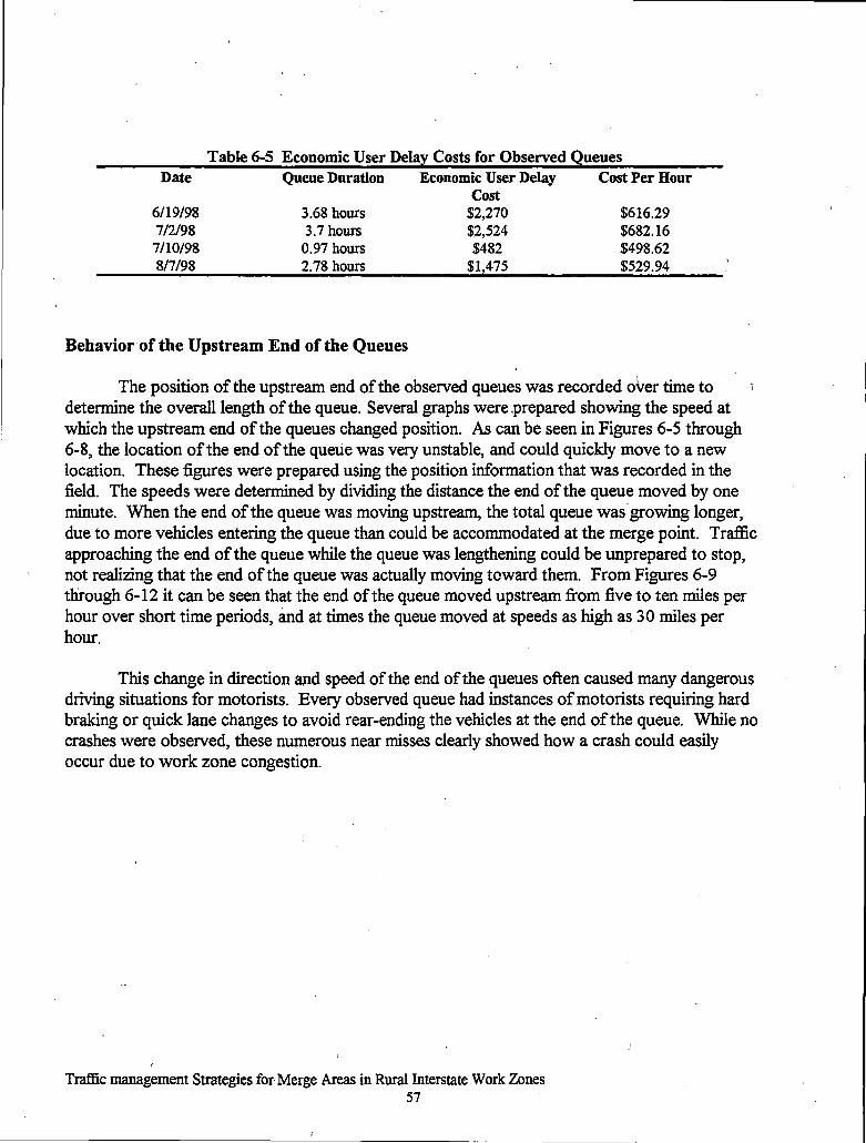
Table 6-5 Economic User Delay Costs for Observed Queues Date

6/19/98 7/2/98

7/10/98 8/7/98

Queue Duration

3.68 hours 3.7 hours

0.97 hours 2.78 hours

Behavior of the Upstream End of the Queues

Economic User Delay Cost

$2,270 $2,524 $482

$1,475

Cost Per Hour

$616.29 $682.16 $498.62 $529.94

The position of the upstream end of the observed queues was recorded o\.-er time to determine the overall length of the queue. Several graphs were ,prepared showing the speed at which the upstream end of the queues changed position. As can be seen in Figures 6-5 through 6-8, the location of the end of the queue was very unstable, and could quickly move to a new location. These figures were prepared using the position information that was recorded in the field. The speeds were determined by dividing the distance the end of the queue moved by one minute. When the end of the queue was moving upstream, the total queue was-growing longer, due to more vehicles entering the queue than could be accommodated at the merge point. Traffic approaching the end of the queue while the queue was lengthening could be unprepared to stop, not realizing that the end of the queue was actually moving toward them. From Figures 6-9 through 6-12 it can be seen that the end of the queue moved upstream from five to ten miles per

' hour over short time periods, and at times the queue moved at speeds as high as 3 0 miles per hour.

This change in direction a.nd speed of the end of the queues often caused many dangerous driving situations for motorists. Every observed queue had instances of motorists requiring hard braking or quick lane changes to avoid rear-ending the vehicles at the end of the queue. While no crashes were observed, these numerous near misses clearly showed how a crash could easily occur due to work zone congestion.

(


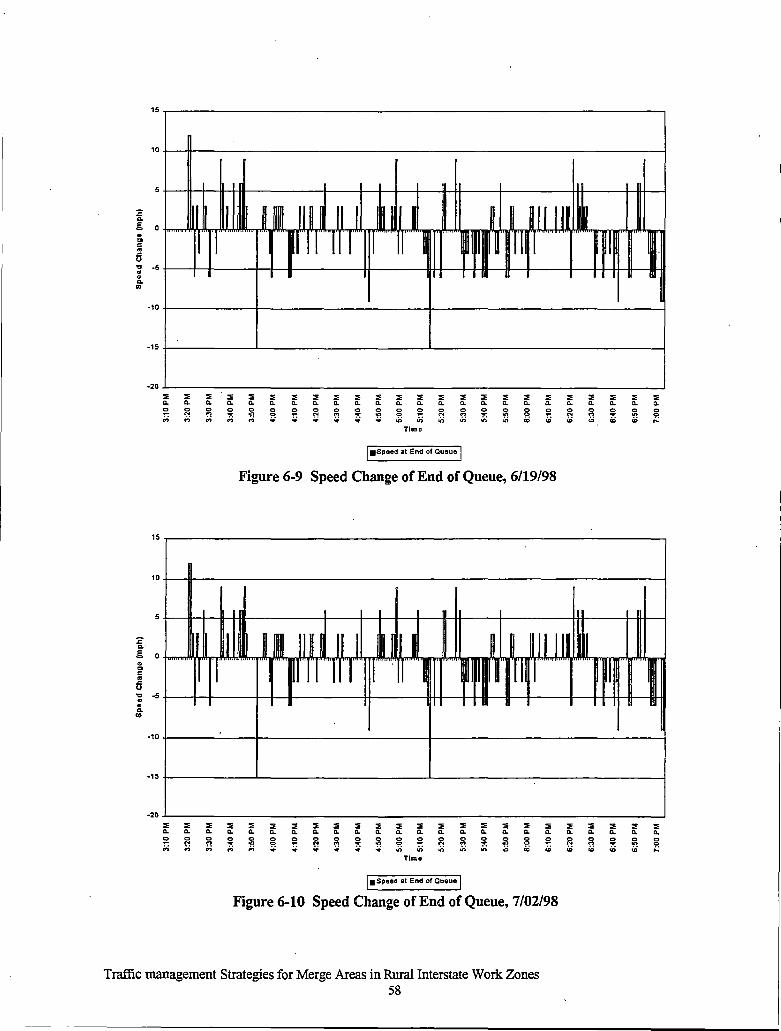
:c "' .5. . "' c .. .c u

15

10

"' -5 " .. "' ..

-10

-15

-20

15

10

5

:c a.·

.5. 0

" "' c .. .c u "' -5 .. .. "' (I)

-10

-15

-20

I l

It .I

I~ ~t~ I ~ I I I u Ill I l l II ·~ ~· l l

:=: :=: :=: :=: :=: :=: 0.. 0.. 0.. 0.. 0.. 0.. 0 0

~ S! :; 0

"' ~ 0 :.r ... .;; .;; ;,; Tlmo

I•Speed at End of Qu~ttue I Figure 6-9 Speed Change of End of Queue, 6/19/98

1~ II ~ I I ~ I I ~ IIIII l l T II .I

~· l l

::E ::E :=: ::E ::E ::E ::E ::E 0.. 0.. 0.. 0.. 0.. 0.. Q, Q,

0 0 0 S! :; ~ 0 0

"' ... "' "' 0 :.r :.r :.r .;; .;; .;; .;; ;,;

Time

I• Speed at End of Queue I Figure 6-10 Speed Change of End of Queue, 7/02/98


I II

~ II

~ 10r---------.---~~--------~----------------------------~ .5. " .. ~ 0~~~~~~~~~~~~~~~~~~~~~~~~~~~~~ u

"' .. .. :-,or-----------------------~----~-------------------.~~~

40

30

20

~ Q.

.5. 10 . Cl c:

" .c u "' 0 . . Q. ..

-10

-20

-30

•

:=: a. ~ ;.;

Time

!•Speed at End ol Queue!

Figure 6-11 Speed Change ofEnd of Queue, 7/10/98

H J tll ~ J II 'l I -~ I ill ~ 1 IW ~ p ·r ,l~l TD I'

:=: :=: :=: :=: :=: :=: :=: :=: :=: :=: :=: Q. a. a. a. a. a. a. a. a. Q. a. ~ 0 0 0 0 ~ 0 :;: ~ 0 0

N ... "' !'! N "' N • • • • "' .;; .;; .;; .;; .;; .;; Time

I•Speed 011t End of Queue j

Figure 6-12 Speed Change of End of Queue, 8/7/98


-- ----------

CHAPTER 7 CONCLUSIONS AND RECOMMENDATIONS

Two significant findings are drawn from this research. First, a more valid value of the capacity of an Iowa interstate work zone has been determined. One example of how this information could be used by the Iowa DOT to improve work zone traffic flow is shown in this chapter. Second, a quantifiable value of the cost imposed on motorists in work zone-related queues at one work zone location has been established, and was shown in the previous chapter. This relatively low delay cost indicates that diversion to relieve congestion at an interstate work zone is not warranted where congestion-based delays are either infrequent or where maximum delays are relatively short (ten minutes). A more serious issue is the speed with which shock waves may move backwards. The upstream growth of shock waves violates the expectation of drivers traveling at freeway speeds and helps to result in unsafe conditions. Given that congestion on rural interstate highways is an inevitable externality of reconstruction and maintenance, highway agencies, like the Iowa DOT, should co~centrate on alerting drivers of approaching queues. Further, we believe that informing drivers of the length of delays they can reasonably expect can help to reduce driver aggressiveness ("road- rage").

WORK ZONE CAPACITY

Based on the data collected at one work zone on Interstate 80 near Davenport, traffic capacity at Iowa's work zone merge areas was found to be from 1,374 to 1,630 passenger cars equivalents per hour when two lanes were reduced to one. One use for this information would be to determine which upcoming work zones would potentially require additional traffic control. Simply examining the previous year's traffic data collected at Automatic Traffic Recorder locations near the planned location of an upcoming work zone could provide insight as to when traffic congestion might occur. For example, Figure 7-1 provides average westbound traffic flow data from the ATR #Ill, near Williamsburg on Interstate 80.(63) These data were taken from the month of July 1997, and averaged by day of the week. As shown in the Figure 7-1, Friday and Sunday afternoons tended, on average, to have enough traffic flow to potentially create congestion based on the capacity levels observed in Davenport. This would indicate that a work zone placed here in future years could expect queues on Friday and Sunday afternoons in July if no additional traffic management efforts are planned. By analyzing traffic levels at future work zone locations in this manner, the DOT could target an enhanced traffic management program to the times when it would be most needed, thereby providing the most effective use of limited resources.

The value of 1,216 vehicles per hour used as the threshold of work zone congestion in Figure 7-1 is taken from Table 6-3, and is the lowest mean capacity value observed at the Davenport location. If this figure had been prepared in passenger car equivalent units, a low value of 1,374 would have been used, again taken from Table 6-3.


------------------------

1600

1400

1200

..:-~ 1000

~ ., 3: 800 0 u:: u = I! 600 ....

400

200

Average Daily Traffic Flows by Day of Week ATR#111,1-80 Near Williamsburg, lA, July 1997

{1,216 Veh/Hr. Threshold of Work Zone Congestion

2 3 4 5 6 7 8 9 10 11 12 13 14 15 16 17 18 19 20 21 22 23 24

Hour of the Day

I --sunday -+-Monday -.-Tuesday -lf-VIIednesday --Thursday --Friday -+-Saturday I Figure 7-1 Using Capacity Values to Determine if Congestion Might Occur

WORK ZONE DELAY COST IMPOSED ON MOTORISTS

This study also found that the four observed queues cost a total of approximately $6,751.00 in economic delay to motorists, as shown in Chapter 6. Hourly delay cost rat~s for the observed queues range from $589.62 to $682.16, with an average value of $606.38 per hour of congestion.

The delays observed at the Davenport location were, in general, never more than about five minutes. For such short delay times, one effective solution could be to employ like the Ohio Travel Time Prediction System which estimates the time required to reach the merge point from a location at or near the end of the queue, and posts the estimate to a changeable message sign. 1 This would provide motorists with information needed to realize that the delay is a short one, and should serve to reduce driver frustration. No other possible improvements seem cost-effective due to the low delay cost and the few times that congestion-based queues were observed.

No crashes were associated with the observed queues, but several near misses were observed as motorists were forced to break to avoid the upstream end of the queue. Any one of these near misses could have resulted in a crash, significantly increasing the cost to the public, crash costs and additional delays for other motorists. Determining an

1 The Ohio Travel Time Prediction System is described in the literature review (see reference (40))


estimate of the number of crashes that result due to work zone congestion would provide an even better picture of the benefit motorists would realize due to improved traffic management. A crash analysis was beyond the scope of this study, and no crashes were observed while the data collection equipment was in place.


REFERENCES

1. "Highway Capacity Manual," Transportation Research Board Special Report 209, Washington, D.C., 1994, p. A-4.

2. Greenshields, B.D., "A Study of Traffic Capacity, Highway Research Board Proceedings, Vol. 14, Washington, D.C., 1934, pp.448- 477.

3. Greenberg, H., "An Analysis of Traffic Flow," Operations Research, Vol. 7, No. 1, pp. 79 - 85, 1959. .

4. Underwood, R.T., "Speed, Volume, and Density Relationships," Quality and Theory of Traffic Flow, Bureau ofHighway Traffic, Yale University, New Haven, CT, 1961, pp 141 - 187.

5. Drake, J.S., Schofer, J., and May, A.D., "A Statistical Analysis of Speed-Density Hypothesis," Proceedings of the Third International Svmposium on Theory of Traffic Flow, New York, NY, June, 1965, pp. 112- 117.

6. Gurlough, D.L.,' and Huber, M.J., "Traffic Flow Theory: A Monograph," Transportation Research Board Special Report 165, Washington, D.C., 1975, p. 51.

7. Hall, F.L., Hurdle, V.F., and Banks, J.H., "Synthesis ofRecent Work on the Nature of Speed-Flow and Flow-Occupancy (Or Density) Relationships on Freeways," Transportation Research Board Record 1365, National Research Council, Washington, D.C., pp. 12 -18.

8. Banks, J.H., "Freeway Speed-Flow Concentration Relationships: More Evidence and Interpretations," Transportation Research Record 1225, National Research Council, Washington, D.C., pp. 53- 60, 1989.

9. Banks, J.H., "Flow Processes at a Freeway Bottleneck," Transportation Research Record 1287, National Research Council, Washington, D.C., pp.83 - 90, 1320.

10. Hall, F.L., andHall, L.M., "Capacity and Speed Flow Analysis of the Queue in Ontario," Transportation Research Record 1287. National Research Council, Washington, D.C., pp. 108- 118, 1990.

11. Chin, H. C. and May, A.D., "Examination of the Speed-Flow Relationship at the Caldecott Tunnel," Transportation Research Record 1320. National Research Council, Washington, D.C., 1991.

12. Wemple, E. A., Morris. A.M., and May, A.D., "Freeway Capacity and Level of Service Concepts," Highway Capacity and Level of Service, Proceedings of the International Svmposium on Highway Capacity, Karlsruhe, Rotterdam: Balkema, pp. 439- 455.

13. Ringer, J. and Urbanik, T., "Study of Freeway Bottlenecks in Texas," Transportation Research Records 1398, National Research Council, Washington, D.C., pp. 31 -41, 1993.

14. Zhou, M., and Hall, F.L., "Investigation of the Speed-Flow Relationship Under Congested Conditions on a Freeway," Presented at the Transportation Research Board Annual Meeting, Washington, D.C., January, 1999.

15. Hall, F.L. and Agyemang-Duah, K., "Freeway Capacity Drop and Definition of Capacity," Transportation Research Record 1320. National Research·council, Washington D.C., 1991.

16. Persaud, B., Yager, S., and Brownlee, R., "Exploration of the Breakdown Phenomenon in Freeway Traffic," Transportation Research Board Annual Meeting, Washington, D.C., January, 1998.


17. Dixon, K.K., Hummer, J.E., and Rouphail, N.M., "Comparison ofRural Freeway Work Zones Queue Length Estimation Techniques: A Case Study," Presented to Transportation Research Board Annual Meeting, Washington, D.C., 1998.

18. Jiang, Y., "Traffic Capacity, Speed, and Queue-Discharge Rate of Indiana's Four-Lane Freeway Work Zones," Presented at the Annual Meeting of the Transportation Research Board, Washington, D.C., 1999 .

. 19. Persaud, B. and Dzbik, L., "Accident Prediction Models for Freeways," Transportation Research Record 1401, pp. 55-60, 1993.

20. Dixon, K.K., and Hummer, J.E., "Capacity and Delay in Major Freeway Construction," Prepared for the North Carolina Department of Transportation by the Center for Transportation Engineering Studies, North Carolina State University, Report No. 23241-94-8, 1995.

21. Memmott, J.L., and Dudek, C.L., "A Model to Calculate the Road User Cost at Work Zones," Prepared by the Texas Transportation Institute, Prepared for the Federal Highway Administration and the Texas Department of Transportation, Austin, TX. Report No. FHW AITX-83/20+292-1, 1982.

22. Lighhill, M.J. and Whitham, G.B., "On Kinematic Waves: Part TI, A Theory on Long Crowded Roads," Proceedings of the Royal Society. Series A. 229 (1178), pp. 317-345, 1955.

23. McShane, W.R. and Roess R.P., Traffic Engineering, New Jersey: Prentice-Hall, Inc. 24. Pal, R. and Sinha, K.C., "Analysis of Crash Rates at Interstate Work Zones in Indiana,"

Transportation Research Record 1529. 1995, pp. 43-53. 25. Khattak, A.J., Khattak, A.J., and Council, F.M., "Analysis of Injury and Non-injury

Crashes in California Work Zones," Presented at the Transportation Research Board Annual Meeting in Washington, D.C., 1999.

26. Byington, S., "Frequency and Location of Rear-End and Side-swipe Work Zone Accidents," Federal Highway Administration, McLean, VA, 1998. (Internal report)

27. Krammes, RA., andLopex, G.O. "Updated Short-TermFreewayWorkZoneLane Closures Capacity Values," Prepared by the Texas Transportation Institute, Prepared for the Federal Highway Administration and the Texas Department of Transportation, Austin, TX, Report No. FHWA/TX-92-/1108-5, 1992.

28. Dudek, C.L. and Richards, S.H., "Traffic Capacity Through Urban Freeway Work Zones in Texas," Transportation Research Record 869, 1982, pp. 14-18.

29. Kermode, R.H., and Myra, W.A., "Freeway Lane Closures," Traffic Engineering Vol. 40, No.5, 1970, pp. 14-18.

30. Richards, S.H., and Dudek, C.L., "Field Evaluation of Traffic Management Strategies for Maintenance Operations in Freeway Middle Lanes," Transportation Research Record 703, 1979, pp. 31-36.

31. Dudek, C.L. and Richards, S.H., "Traffic Management for Middle Lane Maintenance on Urban Freeways," Prepared by the Texas Transportation Institute, Prepared for the Federal Highway Administration and the Texas Department of Transportation, Austin, TX, Report No. FHWAITX-80/3+228-1, 1980.

32. Rouphail, N.M. and Nemeth, Z.A., "Human Factors Considerations as Freeway Construction Lane Closures," ITE Journal, Vol. 52, 1982, pp. 37-44.

33. Byrd, P.S., Geza, P., Jessen, D.S., and McCoy, P.T., "Driver Survey ofthe Late-Merge


Work Zone Traffic Control Strategy," Presented to the 78th Annual Meeting of the Transportation Research Board, Washington, D.C., 1999

34. Rouphail, N.M. and Tiwari, G., "Flow Characteristics at Freeway lane Closures," Transportation Research Record. 1035, 1985, pp. 50-58.

35. Jiang, Y, "Dynamic Predication of Traffic Flow and Congestion at Freeway Work Zones," Presented to the Transportation Research Board at its annual meeting, Washington, D.C., 1999

36. Jiang, Y, "A Model for Estimating Excess User Cost at Highway Workzone," Presented to the Transportation Research Board at its annual meeting, Washington, D.C., 1999.

37. Herstein, H.I., Walczak, W., and Guerra, T.G., "Intelligent Management ofRoadway Closures and Restrictions," Proceedings of the 67th Annual Meeting of the Institute of Transportation Engineers, Boston, MA, 1997.

38. "Des Moines Metropolitan Area ITS Strategic Plan," Prepared by the Center for Transportation Research and Education, Prepared for the Des Moines Area MPO, Des Moines, IA, 1997.

39. Gent, S.J., "Rural Smart Work Zone: A Warning System for Motorists During Interstate Reconstruction Projects," Proceedings of the 68th Meeting of the Institute of Transportation Engineers, Toronto, Ontario, Canada, 1998.

40. Pant, P.O., "Travel Time ~edictions ,System (TIPS) for Freeway Work Zones," Prepared for the Ohio Department ofTransportation by the-University of Cincinnati, 1998.

41. Neudorff: L.G., Galley, D., and Wintermute, J., "The I-95 Corridor Coalition Information Exchange Network," Proceedings of the Annual ITS American Meeting, Washington, o·.c., 1997.

42. Wright, B, Kaliski, J.G., and Pritchard, RD., "Advanced Traveler Information Services for Commercial Vehicle Operators: TruckDesk," Proceedings ofthe Annual ITS America Meeting. Washington, D.C., 1997.

43. "Commercial Vehicle Fleet Management and Information Systems, Phase 1, Interim Report," Prepared by Cambridge Systematics, Inc., ATA Foundation, and the Private Fleet Management Institute, Prepared for the Federal Highway Administration, Report No. DTFH61-93-C-00084, October, 1997, pp. 19- 20.

44. Churchill, B., and Cather, R., and Murphy, D., "San Diego's Prototype Intermodal Transportation Management Center: A Southern California Priority Corridor Showcase Project," Proceedings of the Annual ITS America Meeting, Detroit, MI, 1998.

45. Nookala, M., Dillingham, J.W., Melby, G., and Differt, D., "Smart Work Zone: ITS Operational Test Results," Proceedings of the Annual ITS America Meeting, Detroit, MI, 1998.

46. Boyd, S:J., "A Public- Private Partnership: Minnesota Smart Workzone Case Study," Proceedings of the Annual ITS America Meeting, Washington, D.C., 1999.

47. Private correspondence with Scientex Corporation regarding the ADAPTIRTM~ 1997. 48. Pavis, A., Wilder, W.H., and Hunt, J.F., "Deployment ofRapid Deployment ITS Elements

to Support Construction Management," Proceedings of the 68th Meeting of the Institute of Transportation Engineers, Toronto, Ontario, Canada, 1998.

49. Shapiro, M.S., Pavis, A., Stafford, O.V., and Yogoda, J.H., "Applying ITS Technology for Safer Highway Construction Management," Proceedings of the 68th Meeting of the Institute of Transportation Engineers. Toronto, Ontario, Canada, 1998.


50. Byrd, P.S., Pesti,. G., Jessen, D.S. and McCoy, P.T., "Driver Survey of the Late-Merge Work Zone Traffic Control Strategy," Presented to the Transportation Research Board 78th Annual Meeting, Washington, D.C., 1999.

51. "Freeway Construction Work Zone Safety Enhancement Report," Prepared for the Pennsylvania Department of Transportation, Prepared by Orth-Rodger and Associates, Inc., Philadelphia, PA, 1995.

52. Telephone discussion with Andrzeu Tarko, Assistant Professor of Civil Engineering, Purdue University, April, 1999.

53. Tarko, A.P., Kanipakapatnam, R.K., and Wasson, J.S., "Modeling and Optimization ofthe Indiana Lane Merge Control System on Approaches to Freeway Work Zones," Prepared for the Joint Transportation Research Program, Prepared by the Purdue University, West Lafayette, IN, 1998.

54. Pigman, J.G., Agent, K.R., Deacon, J.A., and Kryscio, R.J., "Evaluation ofUnmanned Radar installations," Transportation Research Record 1244. National Research Council, 1989, pp. 7- 16.

55. Ullman, G.L., and Riesland, D.R., "Catalog of Work Zone Speed Control Methods," prepared for the Texas Department of Transportation by the Texas Transportation Institute, College Station, TX, Report No. FHWA/TX-90/1161-2, 1990.

56. Turochy, R.E., and Sivanandan, R., "Effectiveness ofUnmanned Radar as a Speed Control Technique in Freeway Work Zones," Presented to the Transportation Research Board 77th Annual Meeting, Washington, D.C., 1998.

57. Solarcorp, Movite Journal, Missouri Valley Section, Institute ofTransportation Engineers, December, 1991, p. 4.

58. Special Report 209, Highway Capacity Manual, Third Edition, Transportation Research Board, National Research Council, Washington D.C., 1994.

59. Jiang, Y., Traffic Capacity, Speed, and Queue-Discharge Rate of Indiana's Four-Lane Freeway Work Zones, Presented at the 78th Annual Transportation Research Board Meeting, Washington, D.C., 1999.

60. A Manual on User Benefit Analysis of Highway and Bus-Transit Improvements. American Association of State Highway and Transportation Officials, Washington D.C., 1977. "

61. "Guide to the Economic Evaluation ofHighway Projects," Prepared for the Iowa Department of Transportation, Wilbur Smith Associates, 1993.

62. Bureau ofLabor Statistics Homepage, http:l/146.142.4.24/cgi-bin/surveymost February 4, 1999.

63. Monthly Summary of Traffic Recorder Data, Recorder No. 11130, Station No. 111, July 1997, Provided by the Iowa Department of Transportation, Office of Transportation Data, Ames, IA.


traffic management strategies for merge area in rural

Documents