1

Traffic Signal Control with Partial Grade Separation for

Oversaturated Conditions

By

Ramya Kamineni

August 14th, 2015

A thesis submitted to the

Faculty of the Graduate School of

The State University of New York at Buffalo

in partial fulfillment of the requirements for the degree of

Master of Science

Department of Civil, Structural and Environmental Engineering

2

Table  of  Contents  Acknowledgements ......................................................................................................................... 3  Abstract ........................................................................................................................................... 4  Chapter 1. Introduction ................................................................................................................... 5  

1.1 Background ........................................................................................................................... 5  1.2 Research Objectives .............................................................................................................. 8  1.3 Thesis Organization .............................................................................................................. 8  

Chapter 2. Literature Review ........................................................................................................ 10  2.1. Traffic Signal Control for Oversaturated Conditions ........................................................ 10  2.2. Grade Separation ................................................................................................................ 12  

Chapter 3. Methodology ............................................................................................................... 14  3.1 Optimization Model ............................................................................................................ 14  

3.1.1 General notation and terminology: .............................................................................. 14  3.1.2 Objective Function: ...................................................................................................... 14  3.1.3 Constraints: .................................................................................................................. 17  

Chapter 4. Simulation Results ....................................................................................................... 22  3.1 Simulation Model................................................................................................................ 22  3.2 Synchro Model .................................................................................................................... 23  

Chapter 5. Benefit-Cost Analysis: ................................................................................................ 36  Chapter 6. Conclusions ................................................................................................................. 39  

Future Research ........................................................................................................................ 40  Bibliography ................................................................................................................................. 41  

Deleted:  4

Deleted:  5

Deleted:  6

Deleted:  6

Deleted:  9

Deleted:  9

Deleted:  11

Deleted:  11

Deleted:  13

Deleted:  15

Deleted:  15

Deleted:  15

Deleted:  15

Deleted:  18

Deleted:  23

Deleted:  23

Deleted:  24

Deleted:  35

Deleted:  37

Deleted:  38

Deleted:  39

3

Acknowledgements

I would like to express my gratitude to my advisor Dr. Qing He for his excellent guidance and

support throughout the period of my research and graduate studies. Also for his useful

comments, remarks and help throughout the master thesis. Without his persistent help and

guidance this master thesis would not have been possible.

I would like to thank my committee member Dr. Qiang Wang for her advice and support

throughout my master’s. I would also like to thank my colleagues in the Transportation Systems

Engineering program who have always supported me and helped me and whose association

inspired me to strive for excellence.

I would like to thank my parents Jyothsna, and Gangadhar Kamineni for all the support and love

they share which helped a great deal all my life and also for encouraging me to do masters.

4

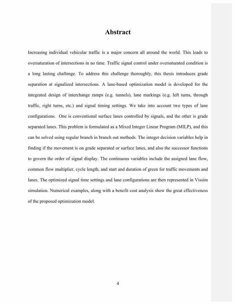
Abstract

Increasing individual vehicular traffic is a major concern all around the world. This leads to

oversaturation of intersections in no time. Traffic signal control under oversaturated condition is

a long lasting challenge. To address this challenge thoroughly, this thesis introduces grade

separation at signalized intersections. A lane-based optimization model is developed for the

integrated design of interchange ramps (e.g. tunnels), lane markings (e.g. left turns, through

traffic, right turns, etc.) and signal timing settings. We take into account two types of lane

configurations. One is conventional surface lanes controlled by signals, and the other is grade

separated lanes. This problem is formulated as a Mixed Integer Linear Program (MILP), and this

can be solved using regular branch in branch out methods. The integer decision variables help in

finding if the movement is on grade separated or surface lanes, and also the successor functions

to govern the order of signal display. The continuous variables include the assigned lane flow,

common flow multiplier, cycle length, and start and duration of green for traffic movements and

lanes. The optimized signal time settings and lane configurations are then represented in Vissim

simulation. Numerical examples, along with a benefit cost analysis show the great effectiveness

of the proposed optimization model.

5

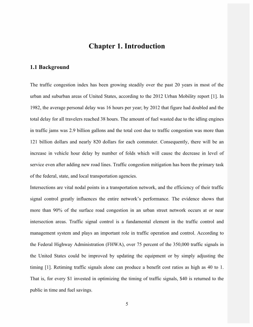
Chapter 1. Introduction

1.1 Background

The traffic congestion index has been growing steadily over the past 20 years in most of the

urban and suburban areas of United States, according to the 2012 Urban Mobility report [1]. In

1982, the average personal delay was 16 hours per year; by 2012 that figure had doubled and the

total delay for all travelers reached 38 hours. The amount of fuel wasted due to the idling engines

in traffic jams was 2.9 billion gallons and the total cost due to traffic congestion was more than

121 billion dollars and nearly 820 dollars for each commuter. Consequently, there will be an

increase in vehicle hour delay by number of folds which will cause the decrease in level of

service even after adding new road lines. Traffic congestion mitigation has been the primary task

of the federal, state, and local transportation agencies.

Intersections are vital nodal points in a transportation network, and the efficiency of their traffic

signal control greatly influences the entire network’s performance. The evidence shows that

more than 90% of the surface road congestion in an urban street network occurs at or near

intersection areas. Traffic signal control is a fundamental element in the traffic control and

management system and plays an important role in traffic operation and control. According to

the Federal Highway Administration (FHWA), over 75 percent of the 350,000 traffic signals in

the United States could be improved by updating the equipment or by simply adjusting the

timing [1]. Retiming traffic signals alone can produce a benefit cost ratios as high as 40 to 1.

That is, for every $1 invested in optimizing the timing of traffic signals, $40 is returned to the

public in time and fuel savings.

6

Traffic signal control under oversaturated conditions is a well-known challenging problem and

has been studied over past decades since [3], [4]. However, very limited progress has been made

for this challenge since the traffic demand exceeds intersection capacity too much in

oversaturation. One potential solution is to use grade separation. Grade separation increases

roadway safety by reducing the vehicle-vehicle and vehicle-pedestrian conflicts. The crossing

traffic is removed from the intersection, thus eliminating the possibility of collisions between

those streams of vehicles. Pedestrians are given greater protection from cars, as there will be

only one line of traffic to cross and more refuge points can be provided at multiple locations.

Removing at-grade intersections with a heavy traffic substantially increases speed and

throughput. Street traffic moves freely over or in tunnel, reducing wait times and increasing

travel speed and capacity of the roadway.

Most importantly, intersections are a large cause of congestion on arterial streets. Signal time

given to each direction dramatically decreases a road’s capacity, increasing the possibility of

congestion and queues. This planned stop-and-go condition reduces safety and increases travel

time for all drivers. Tunneling one of the streets will reduce the conflict caused by intersecting

roadways. The reduced interference will increase the road capacity. Grade-separated

intersections substantially increase capacity by eliminating delay caused by the previous

intersection or railroad. Traffic moves freely and any needed signal timing can be increased by

the lack of a traditional intersection, as signals may only be necessary for accessing the exit and

entrance ramps of the interchange. Elevating one portion of a street or rail crossing improves

safety by eliminating vehicle, train, and pedestrian conflicts. Crossing traffic is minimized; trains

are separated from the roadway; and pedestrians cross traffic less frequently—all decreasing the

likelihood of a collision. The American Association State Highway and Transportation Officials

7

(AASHTO) Highway Safety Manual reports that converting an at-grade, four-leg intersection to

a grade separated interchange reduces injury crashes by 57 percent. Converting a signalized

intersection into a grade-separated interchange reduces injury crashes by 28 percent.

In this thesis, to mitigate oversaturated intersection while considering the cost of grade

separation, we resort to add additional intersection capacity by introducing partial grade

separation (PGS), which allows one or multiple lanes grade separated from other surface lanes

and prevents them from being controlled by signals. A typical PGS example is building a tunnel

under oversaturated intersections. In this case, the tunnel increases the throughput of the

intersection permanently. Compared with traditional traffic signal control, signal control with

PGS helps in smoothing traffic flow with fewer interruptions, achieving higher overall speeds,

and also increasing the capacity of intersection by many folds. Further, we can adopt higher

speed limits on grade separated lanes. In addition, fewer conflicts between traffic movements

reduce the risk of accidents. However, PGS will likely attract more volumes during peak hours.

The demand elasticity of intersection design with PGS will be not considered in the scope of this

thesis. This thesis aims to develop a mathematic model to design traffic signals with PGS and

examine its long-term benefit.

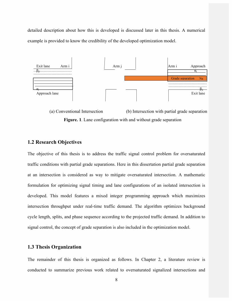
Here in this thesis a signalized intersection with PGS is developed, where both the signal system

and grade separation is adopted, as shown in Figure 1. A partially grade separated intersection

for like 2 or 4 lanes would be more cost effective and also efficient. Now all other movements

will be taken care by the signals. An optimization model is developed after a rigorous analysis in

order to find out lane markings, signal timing settings like the green time, start of green cycle

length. It will also assist in finding out lane settings to be adopted for grade separation. A

8

detailed description about how this is developed is discussed later in this thesis. A numerical

example is provided to know the credibility of the developed optimization model.

1.2 Research Objectives

The objective of this thesis is to address the traffic signal control problem for oversaturated

traffic conditions with partial grade separations. Here in this dissertation partial grade separation

at an intersection is considered as way to mitigate oversaturated intersection. A mathematic

formulation for optimizing signal timing and lane configurations of an isolated intersection is

developed. This model features a mixed integer programming approach which maximizes

intersection throughput under real-time traffic demand. The algorithm optimizes background

cycle length, splits, and phase sequence according to the projected traffic demand. In addition to

signal control, the concept of grade separation is also included in the optimization model.

1.3 Thesis Organization The remainder of this thesis is organized as follows. In Chapter 2, a literature review is

conducted to summarize previous work related to oversaturated signalized intersections and

Exit lane Arm i Arm j Arm i Approach βji αi αi βji Approach lane Exit lane

Grade separation Ng

(a) Conventional Intersection (b) Intersection with partial grade separation

Figure. 1. Lane configuration with and without grade separation

9

grade separation. Chapter 3 introduces the optimization model, describes the model for

computing which is analyzed in order to find out lane settings, lane marking, signal timing

settings like the green time, start of green cycle length. It will also help finding out lane settings

to be adopted for grade separation. Chapter 4 focuses on the microscopic simulation, and the

optimized settings are integrated into Vissim and results are discussed. Chapter 5 discusses about

the benefit cost analysis. Finally, the summary of findings and future research are given in

Chapter 6.

10

Chapter 2. Literature Review

The literature review for the research with two aspects is presented. One is previous studies

related to traffic signal control for oversaturated intersections. The other aspect is the grade

separation. The grade separation, types of grade separation and how they help in handling

congested conditions are reviewed in this chapter.

2.1. Traffic Signal Control for Oversaturated Conditions

Travel demand has rapidly increased over the past decades in urban areas, along with the

growths of population and economic activity; however, due to the limited space available in

urban areas transportation infrastructure has expanded very slowly. Hence, urban transportation

networks have become more crowded and repeatedly develop into gridlock according to [2] and

[3]. When a local queue spills back and spreads over the network very often this state arises,

thereby restricting traffic movements in all other directions ([4],[5],[6]). Signalized intersections

frequently become oversaturated due to the temporal and spatial variation in traffic flow. Under

oversaturated traffic conditions, steady-state models ([7]) may break down when the vehicle

arrival rate exceeds the intersection capacity, leading to the carryover of queues from one cycle

to another. The design of an effective traffic signal timing plan for oversaturated traffic is more

intricate than that for under saturated traffic.

A number of mathematical models have been proposed by many researchers on control variables

in the signal time plan for oversaturated intersections. Some of the remarkable contributions in

early days include: the semi-graphical approach by [2] and [8] where, oversaturation has been

characterized as ‘‘a stopped queue that cannot be completely dissipated during a green cycle” the

work on verification of Dunne–Potts’s phase switching policy for oversaturated flow conditions

11

conducted by [9]; the so-called bang–bang two-stage timing method proposed by [10] and [11]

monograph on traffic signal control theory.

Recently, it is said that oversaturation is due to “traffic queues persist from cycle to cycle either

due to insufficient green splits or because of blockage” and developed a large-scale optimization

models maximizing throughput with constraints on downstream storage capability and green

time utilization ([12]). Another study developed a mixed-integer linear programming approach

for queue length control [13]. [14] developed a dynamic intersection signal control optimization

method for oversaturated condition based on cell-transmission model. [15] presented a hybrid

optimization and rule-based oversaturated control algorithm for isolated signals. [16] and [17]

developed a discrete dynamic model and performance index approach to optimize signal

parameters during the entire period of oversaturated conditions. [18] and [19] proposed negative

offset control strategy, which advances the downstream green in order to flush the residual

queue.

Different with previous approaches, Ding et al. interviewed Traffic control agencies (TCAs),

including police officers, firefighters or other traffic law enforcement officers, who can override

automatic traffic signal control and manually control the traffic at an intersection. They modeled

TCA-based manual traffic signal control and showed that such control methods can mitigate

non-recurrent oversaturated congestions very effectively [20][21].

All the above studies share the common assumption that the geometry design of the intersection

is fixed. In this thesis, we will take into account both designs of grade separation and lane

marking to maximize the intersection capacity under oversaturated conditions.

12

2.2. Grade Separation

Intersections handling a high volume of traffic and pedestrians (and possibly railroads) limit the

capacity of the approaching roads. Grade separation resolves these conflict points and allows an

uninterrupted flow of traffic, while also eliminating the safety threat posed by trains, pedestrians,

or other vehicles. To better allocate scarce regional transportation resources when considering

the construction of grade- separation, [22] created a methodology to provide a consistent

quantitative evaluation of potential locations.  Three primary roadway improvement objectives

are, increased capacity and uninterrupted flow, increased safety. Underpasses increase the

capacity of a roadway by allowing uninterrupted flow in all directions. The intersection

approaches do not come in direct contact but rather bypass each other. Fewer signals are required

to direct traffic, eliminating the queues caused by signals.

At-grade crossings present a barrier to road traffic and the danger of train-vehicle collisions [23].

There was no clear policy concerning the need and the priority for grade separation at crossings.

Simplified tools for rapid crossing evaluation when a crossing potential for grade separation is

reviewed were developed. The evaluation tools include a criterion for preliminary crossing

qualification and a formula for approximate evaluation of economic losses caused by at-grade

crossing functioning. The field measurements and detailed investigation of the 31 most

problematic locations provided a basis for building the tools. Two main factors leading to grade

separation were considered: safety problems at the crossings and road vehicle delay costs. The

cost of accident risk at crossings does not significantly affect their ranking for grade separation.

In consequence, the crossing parameters influence vehicle delays that constitute the basis for the

simplified tools for preliminary crossing evaluation.

13

[26] described a simple analysis for determining whether or not grade separation is warranted for

intersections along urban arterial streets. This determination required the evaluation of user

benefits attributable to operational and design improvements made to arterial intersections.

Comparisons were made between grade-separated interchanges (GSI) and at-grade intersections

(AGI) in terms of the delay, user travel-time costs, and vehicle operating costs. Overall, the

justification for grade separation is dependent on the user benefits offsetting the interchange

construction cost over an assumed design life. A discussion was provided on generalized

warrants for grade separation and on methodologies, used by other, to justify such structures.

Also, this study discussed numerous geometric design considerations for grade-separated

interchanges and other roadway facilities.

A method for determining when traffic flow should be grade separated would be an invaluable

tool for the traffic engineer/planner. [27] facilitated choosing proposed grade separation

improvements on the basis of an evaluation of the reduced delay benefits to the cost of a grade

separation. This methodology can assist decision-makers in determining when grade separations

are appropriate. The analysis was centered on the Federal Highway Administration's model. An

economic analysis that presents the benefit/cost methodology for ranking a grade separation

project was included.

14

Chapter 3. Methodology:

The methodology adopted for this thesis includes three steps. First, an intersection is modelled in

Vissim. The original intersection condition is simulated in Vissim. The second step involves

creating the same scenario in Synchro to optimize the signal timings. These signal timings are

adopted and implemented in Vissim model as the base scenario. The third step develops an

optimization model to obtain lane markings, assignments and signal settings which are again

developed and implemented in Vissim as the test scenarios. All of the test scenarios are

compared to the base to verify the effectiveness of the proposed methods.

3.1 Optimization Model 3.1.1 General notation and terminology:

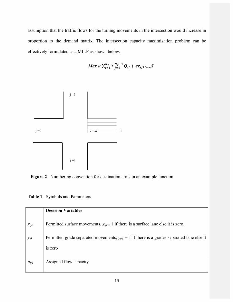
Table 1 lists the parameters used here after and the layout of a typical signalized intersection is

shown in Figure 2 to facilitate the model presentation.

3.1.2 Objective Function:

Because the ultimate objective of operating oversaturated intersections is to accommodate more

cars, capacity maximization is employed as the objective of the integrated optimization model.

The concept of reserved capacity is used to formulae a linear model. Conventionally, the concept

of reserve capacity has been applied to individual signal-controlled intersections, and is

measured by the greatest common multiplier (µ), based on existing total demand

( 𝑸𝒊𝒋𝑵𝑻&𝟏𝒋(𝟏

𝑵𝑻𝒊(𝟏 )[29][30]. The objective also takes in to account the potential savings (S) for

building adjacent grade-separated lanes (𝒛𝒊𝒋𝒌𝒍𝒎𝒏). The model is subject to approach capacity

constraints, cycle time and minimum green constraints and others. Based on the common used

15

assumption that the traffic flows for the turning movements in the intersection would increase in

proportion to the demand matrix. The intersection capacity maximization problem can be

effectively formulated as a MILP as shown below:

Max µ 𝑸𝒊𝒋𝑵𝑻&𝟏𝒋(𝟏

𝑵𝑻𝒊(𝟏 + 𝜺𝒛𝒊𝒋𝒌𝒍𝒎𝒏𝑺

Table 1: Symbols and Parameters

Decision Variables

xijk Permitted surface movements, xijk = 1 if there is a surface lane else it is zero.

yijk Permitted grade separated movements, yijk = 1 if there is a grades separated lane else it

is zero

qijk Assigned flow capacity

j =3

j =2 i

j =1

k = αi

Figure 2. Numbering convention for destination arms in an example junction

16

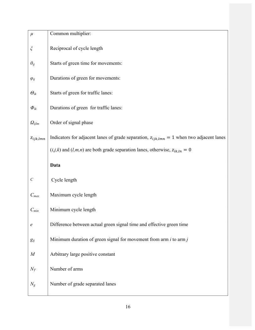
µ Common multiplier:

ξ Reciprocal of cycle length

θij Starts of green time for movements:

φij Durations of green for movements:

Θik Starts of green for traffic lanes:

Φik Durations of green for traffic lanes:

Ωijlm Order of signal phase

𝑧234,678 Indicators for adjacent lanes of grade separation, 𝑧234,678 = 1 when two adjacent lanes

(i,j,k) and (l,m,n) are both grade separation lanes, otherwise, 𝑧24,68 = 0

Data

C Cycle length

Cmax Maximum cycle length

Cmin Minimum cycle length

e Difference between actual green signal time and effective green time

gij Minimum duration of green signal for movement from arm i to arm j

M Arbitrary large positive constant

NT Number of arms

Ng Number of grade separated lanes

17

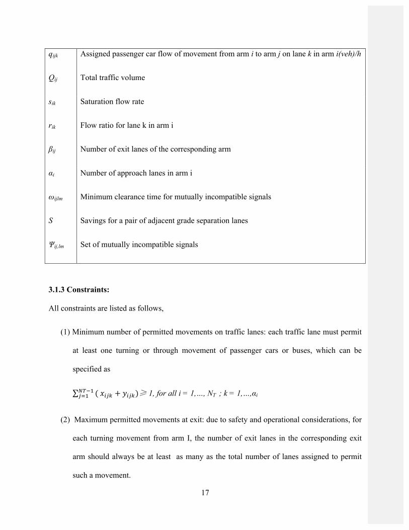
qijk Assigned passenger car flow of movement from arm i to arm j on lane k in arm i(veh)/h

Qij Total traffic volume

sik Saturation flow rate

rik Flow ratio for lane k in arm i

βij Number of exit lanes of the corresponding arm

αi Number of approach lanes in arm i

ωijlm Minimum clearance time for mutually incompatible signals

S Savings for a pair of adjacent grade separation lanes

Ψij,lm Set of mutually incompatible signals

3.1.3 Constraints:

All constraints are listed as follows,

(1)  Minimum number of permitted movements on traffic lanes: each traffic lane must permit

at least one turning or through movement of passenger cars or buses, which can be

specified as

(  𝑥234 + 𝑦234)AB&C  3(C ≥ 1, for all i = 1,…, NT ; k = 1,…,αi

(2)   Maximum permitted movements at exit: due to safety and operational considerations, for

each turning movement from arm I, the number of exit lanes in the corresponding exit

arm should always be at least as many as the total number of lanes assigned to permit

such a movement.

18

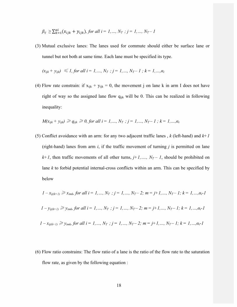
βij ≥   (𝑥234 + 𝑦234)D24(C , for all i = 1,…, NT ; j = 1,…, NT – 1

(3)  Mutual exclusive lanes: The lanes used for commute should either be surface lane or

tunnel but not both at same time. Each lane must be specified its type.

(xijk + yijk) ≤ 1, for all i = 1,…, NT ; j = 1,…, NT – 1 ; k = 1,…,αi

(4)  Flow rate constrain: if xijk + yijk = 0, the movement j on lane k in arm I does not have

right of way so the assigned lane flow qijk will be 0. This can be realized in following

inequality:

M(xijk + yijk) ≥ qijk ≥ 0, for all i = 1,…, NT ; j = 1,…, NT – 1 ; k = 1,…,αi

(5)  Conflict avoidance with an arm: for any two adjacent traffic lanes , k (left-hand) and k+1

(right-hand) lanes from arm i, if the traffic movement of turning j is permitted on lane

k+1, then traffic movements of all other turns, j+1,…., NT – 1, should be prohibited on

lane k to forbid potential internal-cross conflicts within an arm. This can be specified by

below

1 – xij(k+1) ≥ ximk, for all i = 1,…, NT ; j = 1,…, NT – 2; m = j+1,…, NT – 1; k = 1,…,αi-1

1 – yij(k+1) ≥ yimk, for all i = 1,…, NT ; j = 1,…, NT – 2; m = j+1,…, NT – 1; k = 1,…,αi-1

1 – xij(k+1) ≥ yimk, for all i = 1,…, NT ; j = 1,…, NT – 2; m = j+1,…, NT – 1; k = 1,…,αi-1

(6)  Flow ratio constrains: The flow ratio of a lane is the ratio of the flow rate to the saturation

flow rate, as given by the following equation :

19

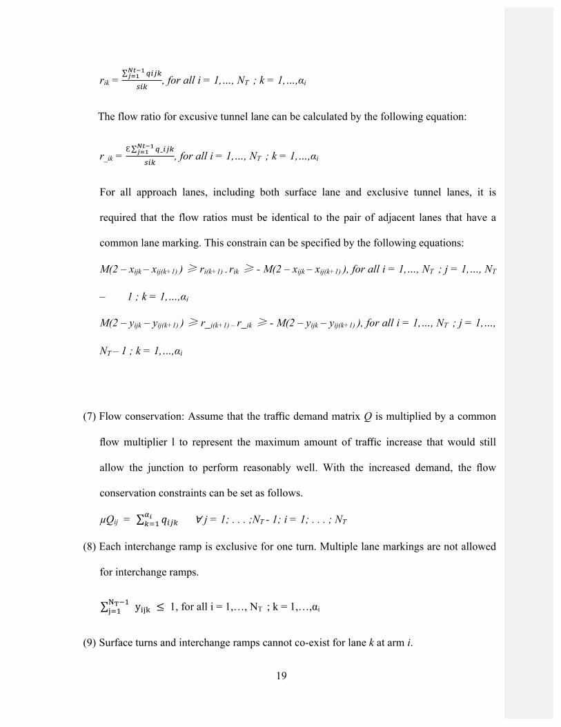
rik = E234FGHI

JKI

L24, for all i = 1,…, NT ; k = 1,…,αi

The flow ratio for excusive tunnel lane can be calculated by the following equation:

r_ik = Ɛ E_234FGHI

JKI

L24, for all i = 1,…, NT ; k = 1,…,αi

For all approach lanes, including both surface lane and exclusive tunnel lanes, it is

required that the flow ratios must be identical to the pair of adjacent lanes that have a

common lane marking. This constrain can be specified by the following equations:

M(2 – xijk – xij(k+1) ) ≥ ri(k+1) - rik ≥ - M(2 – xijk – xij(k+1) ), for all i = 1,…, NT ; j = 1,…, NT

– 1 ; k = 1,…,αi

M(2 – yijk – yij(k+1) ) ≥ r_i(k+1) – r_ik ≥ - M(2 – yijk – yij(k+1) ), for all i = 1,…, NT ; j = 1,…,

NT – 1 ; k = 1,…,αi

(7)  Flow conservation: Assume that the traffic demand matrix Q is multiplied by a common

flow multiplier l to represent the maximum amount of traffic increase that would still

allow the junction to perform reasonably well. With the increased demand, the flow

conservation constraints can be set as follows.

µQij = 𝑞234    DQ4(C ∀ j = 1; . . . ;NT - 1; i = 1; . . . ; NT

(8)  Each interchange ramp is exclusive for one turn. Multiple lane markings are not allowed

for interchange ramps.

                             yTUVWX&C  U(C  ≤ 1, for all i = 1,…, NT ; k = 1,…,αi

(9)  Surface turns and interchange ramps cannot co-exist for lane k at arm i.

20

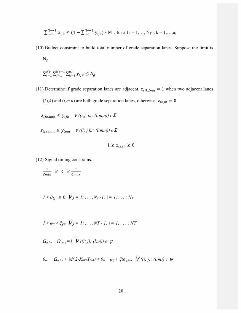
                              xTUVWX&C  U(C ≤ (1 − yTUV

WX&C  U(C ) ∗ M , for all i = 1,…, NT ; k = 1,…,αi

(10)  Budget constraint to build total number of grade separation lanes. Suppose the limit is

Ng

𝑦234DQ4(C

A^&C3(C

A^2(C ≤ 𝑁

(11)  Determine if grade separation lanes are adjacent. 𝑧234,678 = 1 when two adjacent lanes

(i,j,k) and (l,m,n) are both grade separation lanes, otherwise, 𝑧24,68 = 0

                       𝑧234,678 ≤ 𝑦234 ∀ ((i;j, k); (l;m,n)) ϵ Σ

𝑧234,678 ≤ 𝑦678 ∀ ((i; j,k); (l;m,n)) ϵ Σ  

1 ≥ 𝑧24,68 ≥ 0  

(12)  Signal timing constrains:

Cb728

≥ ξ ≥   Cb7cd

1 ≥ 𝜃23  ≥ 0 ∀ j = 1; . . . ;NT -1; i = 1; . . . ; NT

1 ≥ φij ≥ ξgij ∀ j = 1; . . . ;NT - 1; i = 1; . . . ; NT

Ωij,lm + Ωlm,ij =1, ∀ ((i; j); (l;m)) ϵ ψ

θlm + Ωij,lm + M( 2-Xijk-Xlmk) ≥ θij + φij + ξωij,lm, ∀ ((i; j); (l;m)) ϵ ψ

21

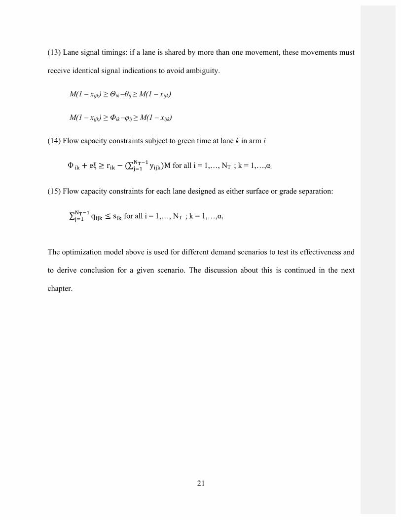
(13) Lane signal timings: if a lane is shared by more than one movement, these movements must

receive identical signal indications to avoid ambiguity.

M(1 – xijk) ≥ Θik –θij ≥ M(1 – xijk)

M(1 – xijk) ≥ Φik –φij ≥ M(1 – xijk)

(14) Flow capacity constraints subject to green time at lane k in arm i

                     ΦTV + eξ ≥ rTV − ( yTUVWX&CU(C )M for all i = 1,…, NT ; k = 1,…,αi

(15) Flow capacity constraints for each lane designed as either surface or grade separation:

qTUVWX&CU(C ≤ sTV for all i = 1,…, NT ; k = 1,…,αi

The optimization model above is used for different demand scenarios to test its effectiveness and

to derive conclusion for a given scenario. The discussion about this is continued in the next

chapter.

22

Chapter 4. Simulation Results

3.1 Simulation Model

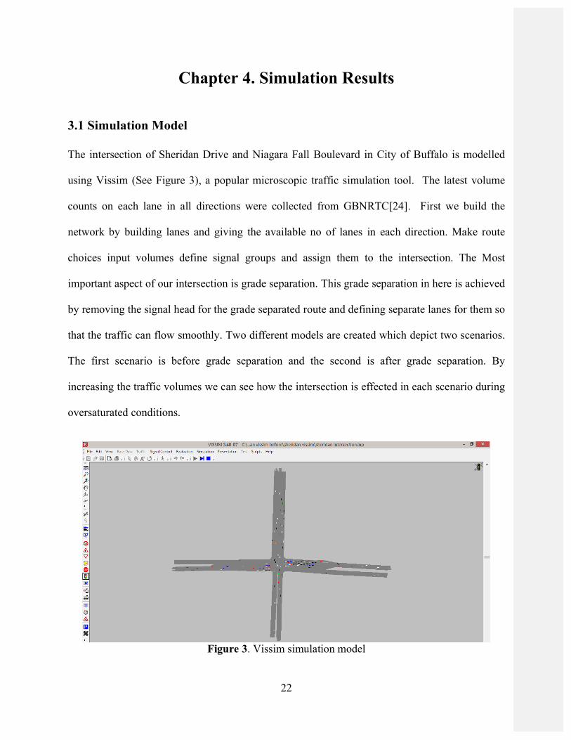
The intersection of Sheridan Drive and Niagara Fall Boulevard in City of Buffalo is modelled

using Vissim (See Figure 3), a popular microscopic traffic simulation tool. The latest volume

counts on each lane in all directions were collected from GBNRTC[24]. First we build the

network by building lanes and giving the available no of lanes in each direction. Make route

choices input volumes define signal groups and assign them to the intersection. The Most

important aspect of our intersection is grade separation. This grade separation in here is achieved

by removing the signal head for the grade separated route and defining separate lanes for them so

that the traffic can flow smoothly. Two different models are created which depict two scenarios.

The first scenario is before grade separation and the second is after grade separation. By

increasing the traffic volumes we can see how the intersection is effected in each scenario during

oversaturated conditions.

Figure 3. Vissim simulation model

23

3.2 Synchro Model

Synchro is a software application for optimizing traffic signal timing and performing capacity

analysis. The software optimizes splits, offsets, and cycle lengths for individual intersections, an

arterial, or a complete network.

Synchro is used for obtain optimized signal timings for the base scenario. The model is created

for three different scenarios, representing different percentage of volume that is 100 percent, 150

percent and 200 percent. The new volumes are induced in the model for each case and the signal

timing is optimized. The optimized signal timings are used in Vissim simulation model as the

base scenario.

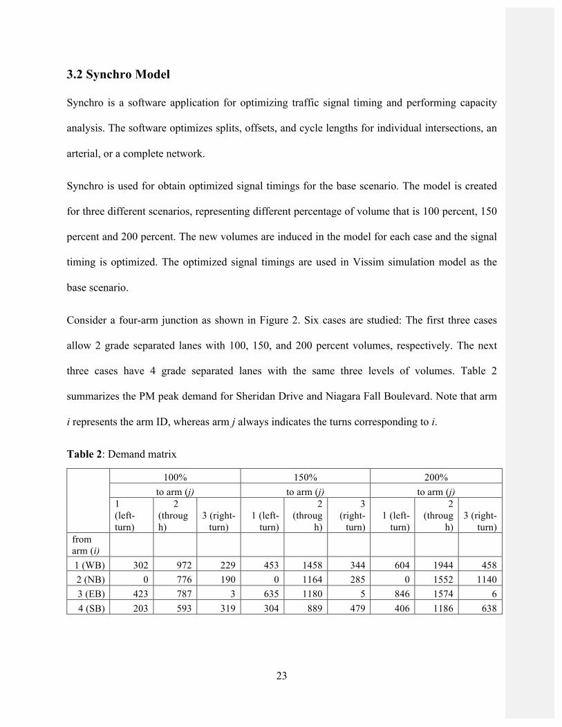
Consider a four-arm junction as shown in Figure 2. Six cases are studied: The first three cases

allow 2 grade separated lanes with 100, 150, and 200 percent volumes, respectively. The next

three cases have 4 grade separated lanes with the same three levels of volumes. Table 2

summarizes the PM peak demand for Sheridan Drive and Niagara Fall Boulevard. Note that arm

i represents the arm ID, whereas arm j always indicates the turns corresponding to i.

Table 2: Demand matrix

100% 150% 200% to arm (j) to arm (j) to arm (j)

1 (left-turn)

2 (through)

3 (right-turn)

1 (left-turn)

2 (throug

h)

3 (right-

turn) 1 (left-

turn)

2 (throug

h) 3 (right-

turn) from arm (i) 1 (WB) 302 972 229 453 1458 344 604 1944 458 2 (NB) 0 776 190 0 1164 285 0 1552 1140 3 (EB) 423 787 3 635 1180 5 846 1574 6 4 (SB) 203 593 319 304 889 479 406 1186 638

24

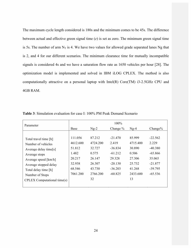
The maximum cycle length considered is 180s and the minimum comes to be 45s. The difference

between actual and effective green signal time (e) is set as zero. The minimum green signal time

is 5s. The number of arm NT is 4. We have two values for allowed grade separated lanes Ng that

is 2, and 4 for our different scenarios. The minimum clearance time for mutually incompatible

signals is considered 4s and we have a saturation flow rate as 1650 vehicles per hour [28]. The

optimization model is implemented and solved in IBM iLOG CPLEX. The method is also

computationally attractive on a personal laptop with Intel(R) Core(TM) i3-2.5GHz CPU and

4GB RAM.

Table 3: Simulation evaluation for case I: 100% PM Peak Demand Scenario

Parameter 100% Base Ng-2 Change % Ng-4 Change%

Total travel time [h] 111.056 87.212 -21.470 85.999 -22.562

Number of vehicles 4612.600 4724.200 2.419 4715.400 2.229

Average delay time[s] 51.812 32.727 -36.834 30.890 -40.380

Average stops 1.482 0.575 -61.212 0.506 -65.866

Average speed [km/h] 20.217 26.147 29.328 27.306 35.065

Average stopped delay 32.938 26.307 -20.130 25.732 -21.877

Total delay time [h] 68.546 43.730 -36.203 41.268 -39.795

Number of Stops 7061.200 2766.200 -60.825 2433.600 -65.536

CPLEX Computational time(s) 32 13

25

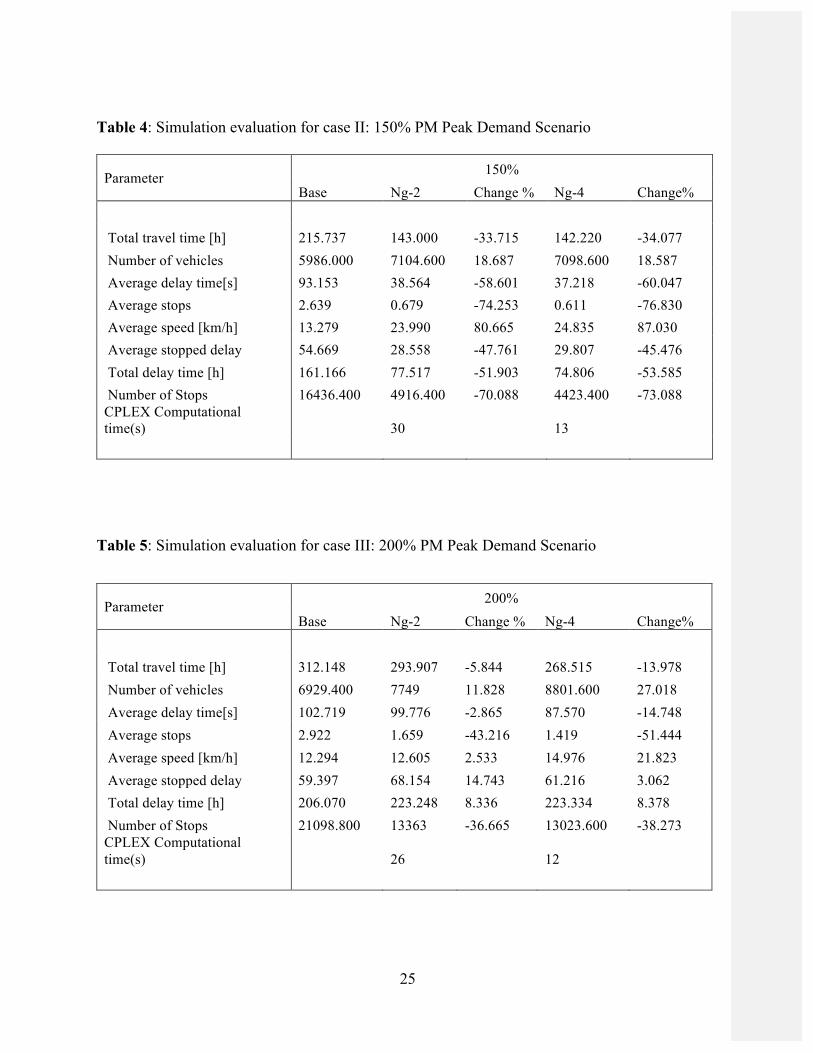
Table 4: Simulation evaluation for case II: 150% PM Peak Demand Scenario

Parameter 150% Base Ng-2 Change % Ng-4 Change%

Total travel time [h] 215.737 143.000 -33.715 142.220 -34.077 Number of vehicles 5986.000 7104.600 18.687 7098.600 18.587 Average delay time[s] 93.153 38.564 -58.601 37.218 -60.047 Average stops 2.639 0.679 -74.253 0.611 -76.830 Average speed [km/h] 13.279 23.990 80.665 24.835 87.030 Average stopped delay 54.669 28.558 -47.761 29.807 -45.476 Total delay time [h] 161.166 77.517 -51.903 74.806 -53.585 Number of Stops 16436.400 4916.400 -70.088 4423.400 -73.088 CPLEX Computational time(s) 30 13

Table 5: Simulation evaluation for case III: 200% PM Peak Demand Scenario

Parameter 200% Base Ng-2 Change % Ng-4 Change%

Total travel time [h] 312.148 293.907 -5.844 268.515 -13.978 Number of vehicles 6929.400 7749 11.828 8801.600 27.018 Average delay time[s] 102.719 99.776 -2.865 87.570 -14.748 Average stops 2.922 1.659 -43.216 1.419 -51.444 Average speed [km/h] 12.294 12.605 2.533 14.976 21.823 Average stopped delay 59.397 68.154 14.743 61.216 3.062 Total delay time [h] 206.070 223.248 8.336 223.334 8.378 Number of Stops 21098.800 13363 -36.665 13023.600 -38.273 CPLEX Computational time(s) 26 12

26

The base represents the case where the existing real-world intersection layout is considered at the

current intersection. So this scenario will not have any grade separated lanes but it has optimized

signal settings by Synchro. For our proposed models, the optimized lane configurations and

signal timings are implemented in Vissim and results are obtained from simulation accordingly.

The results of evaluation from each scenario are presented in Table 3-5. As we can see from each

scenario, the savings in disutility are remarkable after adding grade separated lanes. Considering

case I that is 100% volume scenario, shown in Table 3, we have a 21 percent and 22 percent

decrease in travel time for two (Ng-2) and four (Ng-4) grade separated lanes respectively. But

the throughput is almost the same as the base scenario and the optimized case only shows a slight

increase of 2 percent for each case. As one can see, there is a decrease in average delay by 37

percent for Ng-2 and 40 percent for Ng-4 which indicates that model performs well. We can also

see from the table that there is a significant amount of decrease in number of stops for this

scenario.

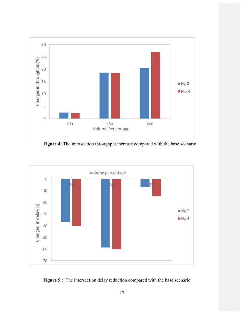
Now moving on to case II which is 150 percent volume, the results are illustrated in Table 4. As

we can see from table there is significant change in average delay values in this case compared to

base case and case I, which comes out to be 58 percent and 60 percent for Ng-2 and Ng-4,

respectively. The average speed also are increased by a great amount with a percentage as high

as 87 percent for Ng-4. The number of stops in this case decreases by 70 percent from 16436 to

4916. For case III we have 200 percent increase in volume, and the results for this scenario are

shown in Table 5. Throughput for Ng-4 increases by 27 percent which is highest of all the

scenarios. However, the average reductions, 3 and 14 percent respectively, are not as significant

as case II.

27

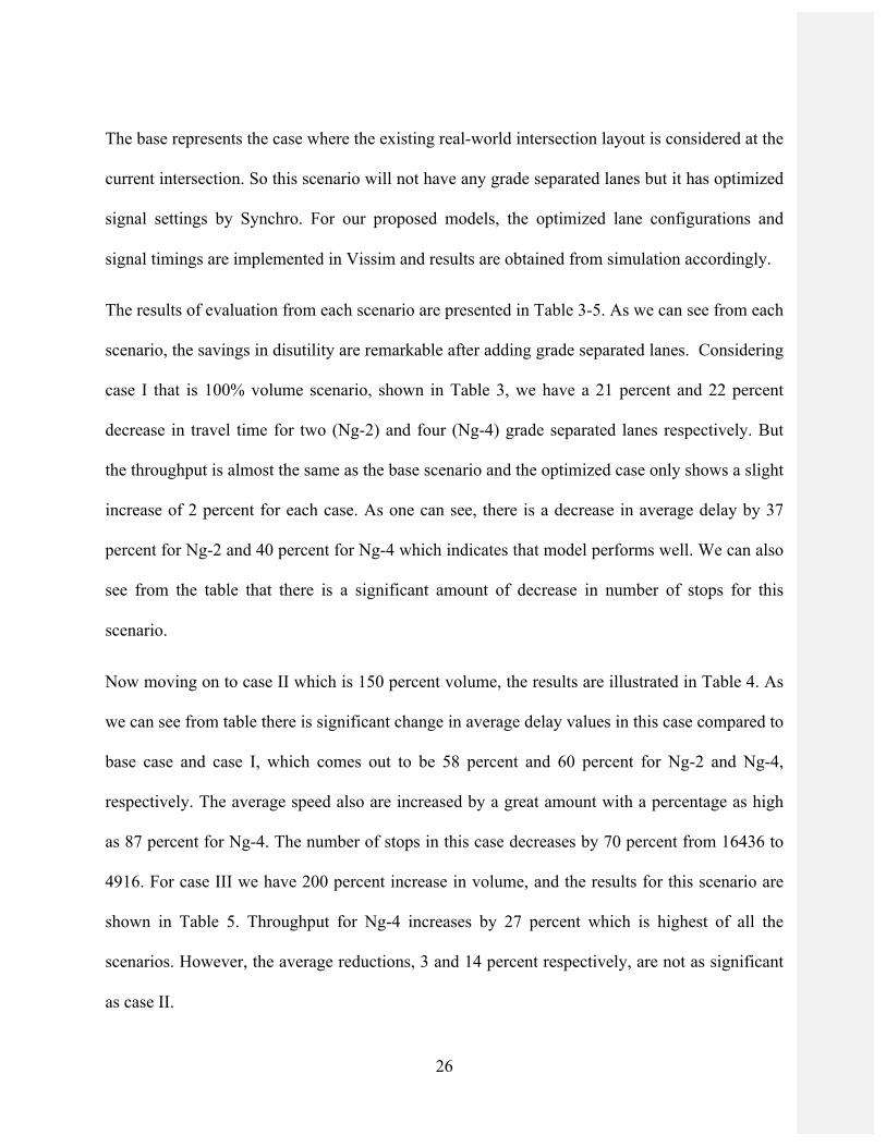
Figure 4: The intersection throughput increase compared with the base scenario

Figure 5 : The intersection delay reduction compared with the base scenario.

28

A comparison between Ng-4and Ng-2 is represented in the Figure 4 and Figure 5 above. The

throughput increases for each case as one can see in Figure 4. There is only a 2 percent increase

for the original 100 percent volume case compared to the base, since it is not an oversaturated

condition. The percent change increases from 2 percent to 19 percent with the Ng2 and Ng4

cases for the 150 percent of PM peak volume. The throughput for the case III came out to

increase by an amount of 27 percent from 6929 to 8801 under Ng-4 scenario.

29

(a)   (b)

(c) (d)

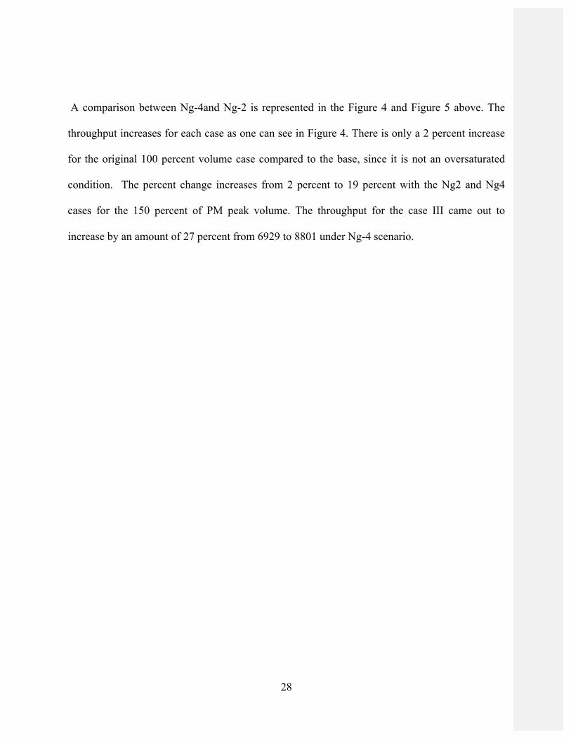
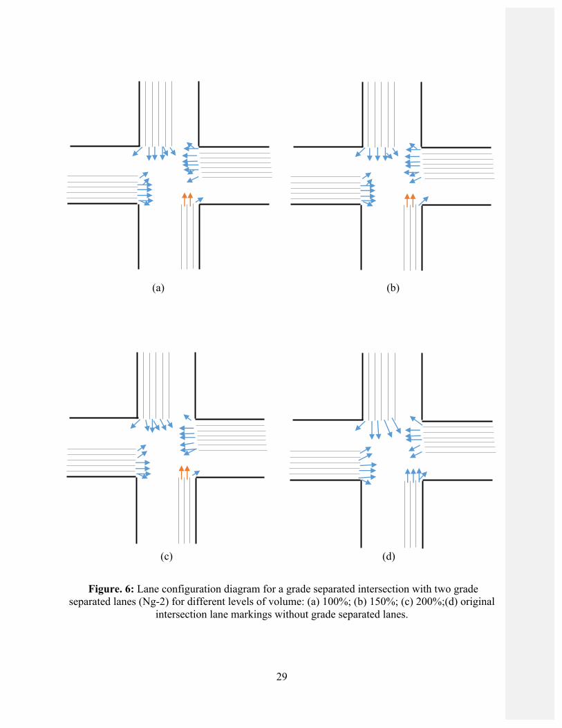
Figure. 6: Lane configuration diagram for a grade separated intersection with two grade

separated lanes (Ng-2) for different levels of volume: (a) 100%; (b) 150%; (c) 200%;(d) original intersection lane markings without grade separated lanes.

30

(a) (b)

(c) (d)

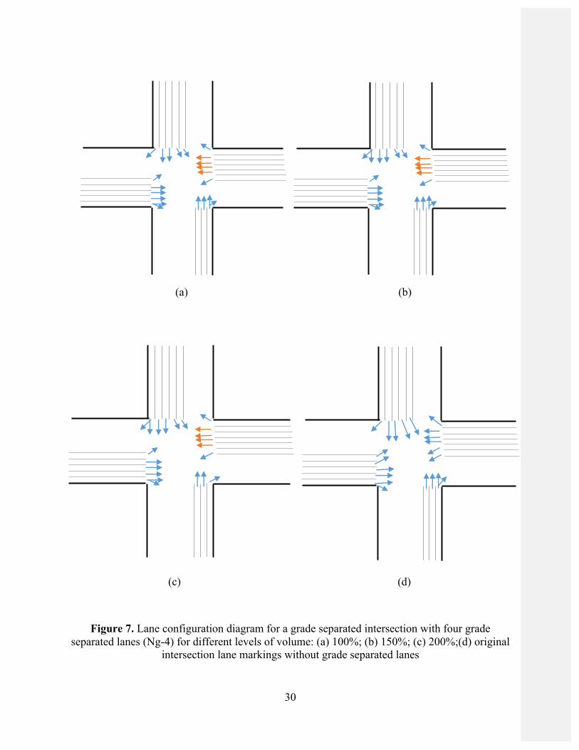
Figure 7. Lane configuration diagram for a grade separated intersection with four grade separated lanes (Ng-4) for different levels of volume: (a) 100%; (b) 150%; (c) 200%;(d) original

intersection lane markings without grade separated lanes

31

The lane settings and configurations are very critical in the design of an intersection to maximize

the possible throughput. The lane configurations for Ng-2 can be found in Figure 6. As we can

see we have two grade separated lanes in arm 2 which are represented in orange color. In this

case, except for northbound right-turn, all northbound traffic has been accounted by grade

separation due to the fact that no northbound left-turn demand exists. Therefore, the signal

timing settings do not have to take into account northbound traffic at all.

The lane configuration for a Ng-4 intersection can be seen in Figure 7. Same convention can be

followed to obtain the lane configurations for each of the cases in Figure 7(a), (b) and (c). As we

can see both the cases arm one has four grade separated lanes from Figure 7. The results show

that there is a through lane added for case I and II for arm 2 which is not present for case III. The

second left is made a through lane in the second scenario. Comparing the base case to other cases

for Ng-2, through lanes are added to the second left turn in all the arms. For Ng-4 one of the left

is made through in 3rd arm and a through is added for right lane in 4th arm. These are the major

changes associated with the lane configuration.

32

(a)

(b)

(c)

33

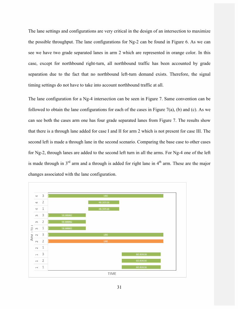
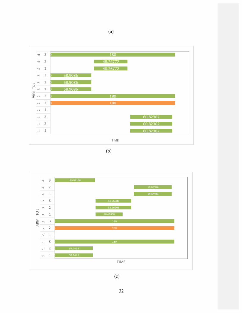
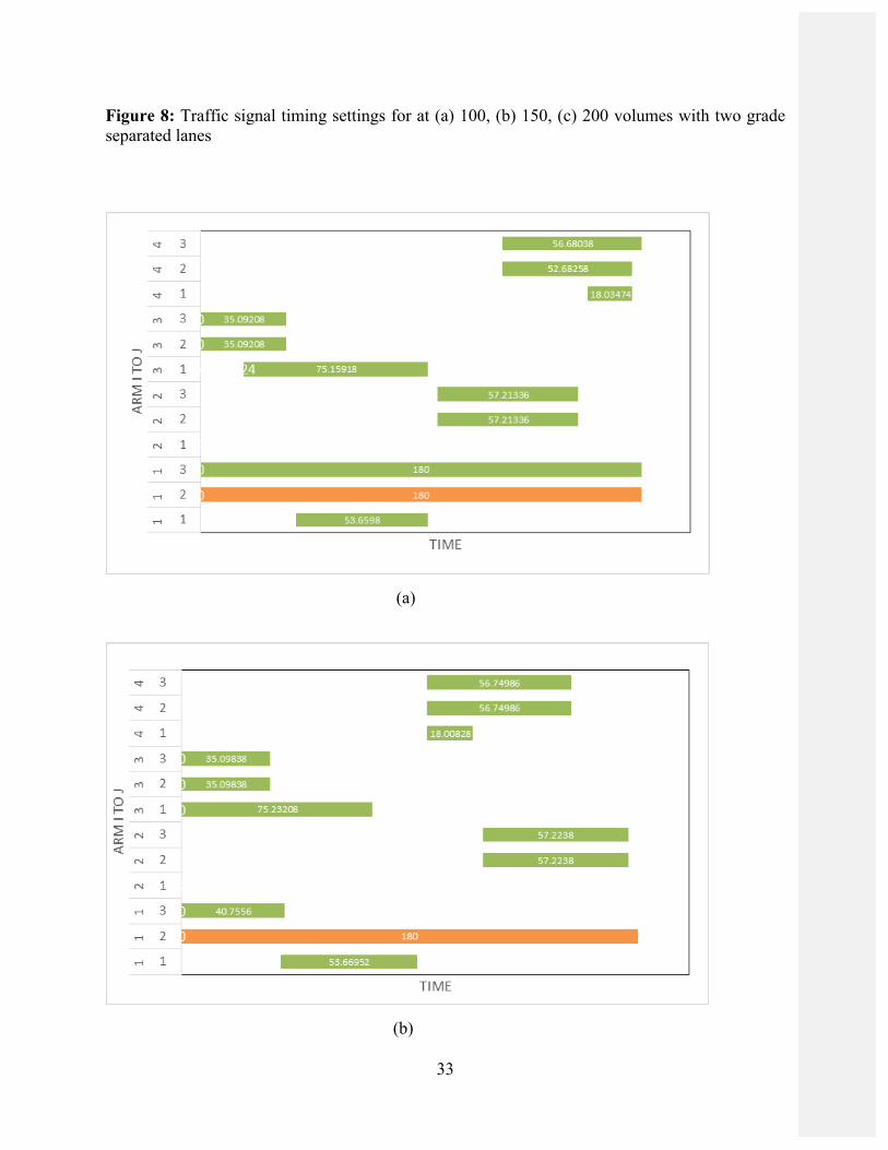
Figure 8: Traffic signal timing settings for at (a) 100, (b) 150, (c) 200 volumes with two grade separated lanes

(a)

(b)

34

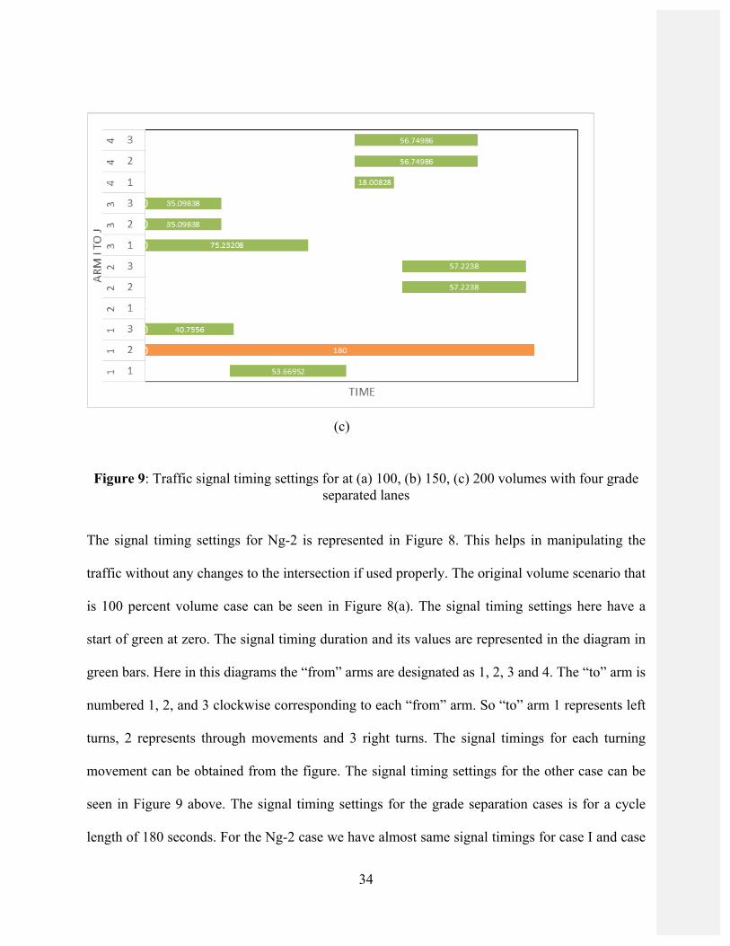
(c)

Figure 9: Traffic signal timing settings for at (a) 100, (b) 150, (c) 200 volumes with four grade separated lanes

The signal timing settings for Ng-2 is represented in Figure 8. This helps in manipulating the

traffic without any changes to the intersection if used properly. The original volume scenario that

is 100 percent volume case can be seen in Figure 8(a). The signal timing settings here have a

start of green at zero. The signal timing duration and its values are represented in the diagram in

green bars. Here in this diagrams the “from” arms are designated as 1, 2, 3 and 4. The “to” arm is

numbered 1, 2, and 3 clockwise corresponding to each “from” arm. So “to” arm 1 represents left

turns, 2 represents through movements and 3 right turns. The signal timings for each turning

movement can be obtained from the figure. The signal timing settings for the other case can be

seen in Figure 9 above. The signal timing settings for the grade separation cases is for a cycle

length of 180 seconds. For the Ng-2 case we have almost same signal timings for case I and case

35

II but we have a slight change in timings for case III. However for the Ng-4 case we have the

same signal timings for all the cases except that the start of green signal timings is different for

each case. Since there is an increased number of through lanes compared to the base case, the

signal timings for the through lanes increased. These timings are used for obtaining the results by

importing the values into Vissim simulation software.

36

Chapter 5 Benefit-Cost Analysis

Benefit-cost analysis (BCA) is conducted to evaluate the economic benefits of implementing the

grade separated traffic signal system in place of traditional traffic signal system BCA is often

used by governments and other organizations, such as private sector businesses, to appraise the

desirability of a given policy. It is an analysis of the expected balance of benefits and costs,

including an account of foregone alternatives and the status quo. BCA helps predict whether the

benefits of a policy outweigh its costs, and by how much relative to other alternatives (i.e. one

can rank alternate policies in terms of the cost–benefit ratio). Generally, accurate cost–benefit

analysis identifies choices that increase welfare from a utilitarian perspective. Assuming an

accurate BCA, changing the status quo by implementing the alternative with the lowest cost–

benefit ratio can improve efficiency. An analyst using BCA should recognize that perfect

appraisal of all present and future costs and benefits is difficult, and while BCA can offer a well-

educated estimate of the best alternative, perfection in terms of economic efficiency and social

welfare are not guaranteed.

As an example, we conduct BCA analysis for 100% of PM peak volume with two grade

separated lanes (Ng-2). Several assumptions are made as follows:

•   We will build a 0.5 mile two lane tunnel.

•   The tunnel cost is 75 million dollars per mile.[25]

•   The value of travel time is $16.79 per hour (Texas Transportation Institute, 2012)

[1].The peak hour volumes and the travel time values are obtained from field and

simulation, respectively.

•   Annual volume increases by 2%.

37

•   Tunnel maintenance cost is 169 thousand per year [31].

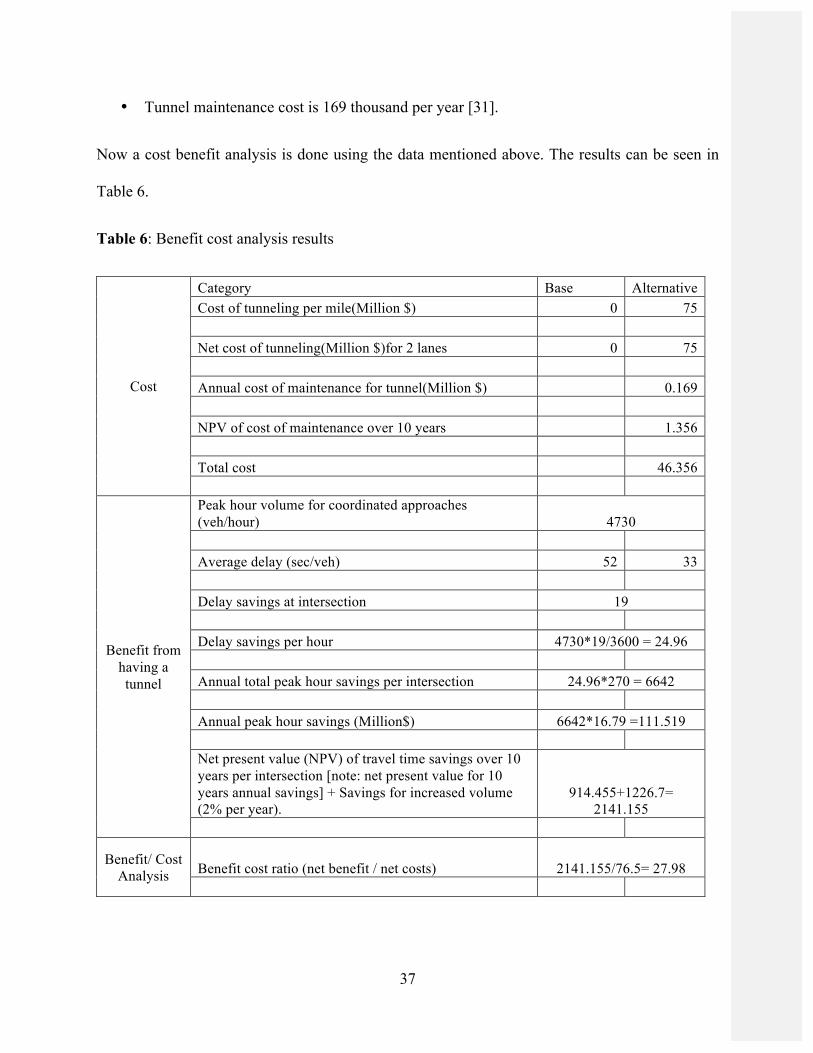
Now a cost benefit analysis is done using the data mentioned above. The results can be seen in

Table 6.

Table 6: Benefit cost analysis results

Cost

Category Base Alternative Cost of tunneling per mile(Million $) 0 75 Net cost of tunneling(Million $)for 2 lanes 0 75 Annual cost of maintenance for tunnel(Million $) 0.169 NPV of cost of maintenance over 10 years 1.356 Total cost 46.356

Benefit from having a tunnel

Peak hour volume for coordinated approaches (veh/hour) 4730 Average delay (sec/veh) 52 33 Delay savings at intersection 19 Delay savings per hour 4730*19/3600 = 24.96 Annual total peak hour savings per intersection 24.96*270 = 6642 Annual peak hour savings (Million$) 6642*16.79 =111.519 Net present value (NPV) of travel time savings over 10 years per intersection [note: net present value for 10 years annual savings] + Savings for increased volume (2% per year).

914.455+1226.7= 2141.155

Benefit/ Cost Analysis Benefit cost ratio (net benefit / net costs) 2141.155/76.5= 27.98

38

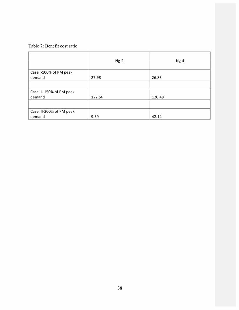
Table 7: Benefit cost ratio

   Ng-­‐2   Ng-­‐4  

Case  I-­‐100%  of  PM  peak  demand   27.98   26.83  

           Case  II-­‐  150%  of  PM  peak  demand   122.56   120.48  

           Case  III-­‐200%  of  PM  peak  demand   9.59   42.14  

39

Chapter 6. Conclusions:

In this thesis, a lane-based optimization method for the integrated design of lane markings and

signal settings for isolated junctions has been presented. Both traffic and pedestrian movements

have been considered in a unified framework. The capacity maximization have been considered.

These problems have been formulated as a MILP, which can be solved by a standard branch-and-

bound routine. The binary variables (i.e., the permitted movements on traffic lanes and successor

functions to govern the order of signal displays) and the continuous variables (i.e., the assigned

lane flows, common flow multiplier, cycle length, as well as starts and durations of green for

traffic movements, lanes and pedestrian crossings) have been defined. A set of constraints have

been set up to ensure feasibility and safety of the resulting optimal lane markings and signal

settings. Simulations are done in Vissim.

Numerical examples have been given to demonstrate the effectiveness of the proposed method.

The method is also computationally attractive. There is a good savings in delay for each

scenario. The first two cases (with 100% and 150% of PM peak volume, respectively) of two

lane grade separation (Ng-2) has a 36 percent and 58 percent savings in the delay. The case III

(with 200% of PM peak volume) has a delay savings of 7 percent because of extreme heavy

traffic. But the case with four lane grade separated (Ng-4) has more delay savings compared to

the (Ng-2) which sums up to be 40 percent for case I, 60 percent for case II and 15 percent for

case III. There is also a significant increase in throughput for Ng-4, initially for case I it

increased by 3 percent. But for case II it increased by 18 percent and for case III it is as huge as

27 percent. From the benefit cost analysis we have benefit cost ratio for each of these case. For

Ng-2 with case I, we have 27.98 from Table 6. In the same way it is calculated for other cases.

40

For Ng-2 with case II, it is 122.56 and Ng-2 with case III has a value of 9.59. For Ng-4, it comes

out to be 26.83 for case I, 120.48 percent for case II and 42.14 for case III.

Future Research:

The proposed optimization model can be used for finding the signal time settings, lane

markings, lane settings for a series of intersections on an arterial. The goal is to maximize the

flow capacity along an oversaturated corridor. This can also be extended to an entire network.

The decentralized control logic in this dissertation shows the potential to extend the proposed

approach to larger networks.

There is also a need to develop improved traffic flow prediction and queue prediction models.

The application of more sophisticated traffic predication model can enhance the capabilities of

the proposed model. The validity of the model has been verified by various simulation studies.

Field test is desired for further evaluating the performance of the proposed algorithm.

One more thing to address in future research is the location of grade separated intersection. The

location is important aspect for adopting a grade separate lane because it is influenced by the

traffic volumes. Also if it is a residential area grade separation might cause land use impact, and

increase in volumes in the neighborhood due to grade separation. So addressing this case will

help solve the problem.

41

Bibliography

1. Schrank. D, Eisele. B, Lomax. T, “TTI’s 2012 Urban Mobility Report“ http://mobility.tamu.edu/ums, accessed on August 10, 2015

2. Liu. C. C , “Bandwidth-constrained delay optimization for signal systems,” Int. Transp. Eng.

J., vol. 58, no. 12, pp. 21–26, Dec. 1988.

3. Gazis. D. C, “Optimum control of a system of oversaturated intersections,” Oper. Res., vol.

12, no. 6, pp. 815–831, 1964

4. Daganzo C. F, “The nature of freeway gridlock and how to prevent it,” in Proc. 13th Int.

Symp. Transp. Traffic Theory, Amsterdam, The Netherlands, pp. 629–646, 1996.

5. Daganzo C. F, “Urban gridlock: Macroscopic modeling and mitigation approaches,” Transp.

Res. B, vol. 41, no. 1, pp. 49–62, Jan. 2007.

6. Schmocker. J, Ahuja S, and M. Bell, “Multi-objective signal control of urban junctions–

Framework and a London case study,” Transp. Res. C, vol. 16, no. 4, pp. 454–470, Aug. 2008.

7. Koonce, P., Rodegerdts, L., Lee, K., Quayle, S., Beaird, S., Braud, C., Bonneson, J., Tarnoff,

P., Urbanik, T., 2008. Traffic Signal Timing Manual, Federal Highway Administration Report:

FHWA-HOP-08-024.

8. Gazis, D.C., Potts, R.B., 1965. The oversaturated intersections. In: Proceedings of the Second

International Symposium on the Theory of Road Traffic Flow, pp. 221–237.

9. Green, D.H., 1967. Control of oversaturated intersections. Operations Research 18 (2), 161–

173.

42

10. Michalopoulos, P.G., Stephanopoulos, G., 1977b. Oversaturated signal systems with queue

length constraints – II systems of intersections. Transportation Research 11, 423–428.

11. Newell, G.F., 1989. Theory of highway traffic signals. Research Report UCB-ITS-CN-89-1.

University of California at Berkeley.

12. Abu-Lebdeh, G., Benekohal, R.F., 2000. Genetic algorithm for traffic signal control and

queue management of oversaturated two-way arterials. Transportation Research Record (1727),

61–67.

13. Lieberman, E.B., Chang, J., Prassas, E.S., 2000. Formulation of real-time control policy for

oversaturated arterials. Transportation Research Record (1727), 68–78.

14. Lo, H.K., Chow, A.H., 2004. Control strategies for oversaturated traffic. Journal of

Transportation Engineering 130 (4), 466–478.

15. Li, Prevedouros. H, P.D., 2004. Traffic adaptive control for oversaturated isolated

intersections: model development and simulation testing. Journal of Transportation Engineering

130 (5), 594–601.

16. Chang, T.H., Lin, J.T., 2000. Optimal signal timing for an oversaturated intersection.

Transportation Research Part B 34 (6), 471–491.

17. Chang, T.-H., Sun, G.Y., 2004. Modeling and optimization of an oversaturated signalized

network. Transportation Research Part B 38 (8), 687–707

18. Pignataro, L.J., McShane, W.R., Crowley, K.W., 1978. Traffic control in oversaturated street

networks. National Cooperative Highway Research Program Report 194. Transportation

Research Board, Washington, DC.

43

19. Rathi, A.K., 1988. Control scheme for high density traffic sectors. Transportation Research

Board 22B (2), 81–101.

20. Ding, N.*, Q. He , C. Wu, and J. Fetzer*, “Modeling Traffic Control Agency Decision

Behavior for Multi-modal Manual Signal Control under Event Occurrences”, to appear in IEEE

Transactions on Intelligent Transportation Systems

21. Ding, N.*, Q. He, and C. Wu, “Performance Measures of Manual Multi-Modal Traffic Signal

Control”, Transportation Research Record: Journal of the Transportation Research Board, No.

2438, 2014, pp 55-63

22. Michael H. Schrader and John R. Hoffpauer, 2001. Methodology for Evaluating Highway-

Railway Grade Separations. Transportation Research Record (1754), 77–80.

23. Hakkert  A. , Gitelman V. , 1997. Development of Evaluation Tools for Road-Rail Crossing

Consideration for Grade Separation. Transportation Research Record (1605), pp. 96–105.

24. Transportation data management system, GBNRTC

http://gbnrtc.ms2soft.com/tcds/tsearch.asp?loc=Gbnrtc&mod=

25. Efron. N, Read. M, 2012. “Analyzing international tunnel costs”. Worcester Polytechnic

Institute.

26. Lang. L, Machemehl RB, 1995. “Congress Avenue Regional Arterial Study: Grade

Separations”. swutc.tamu.edu.

27. Rymer B, Urbanik II, 1989. “Intersection, Diamond, and Three-Level Diamond Grade

Separation Benefit-Cost Analysis Based on Delay Savings”. Transportation Research Record.

28. Traffic Engineering, by Roess, Prassas and McShane, Fourth Edition, Prentice-Hall, 2011.

44

29. Wong C.K, Wong S.C, 2003. “Lane-based optimization of signal timings for isolated

junctions”. Transportation Research Part B 37, 63-84.

30. Ma, W., Head K.L., Feng, Y., 2014. “Integrated optimization of transit priority operation at

isolated intersections: A person-capacity-based approach”. Transportation Research Part C 40,

49-62.

31.Richard. W, Gary. F, 2003.” Comparing Costs of Options for Reconstructing the 12th and

27th Avenue Bridges Over the Miami River.” Miami river commission.