training manual on the integrated vulnerability assessment

Training Manual on the Integrated Vulnerability Assessment Methodology

Regional Initiative for the Assessment of Climate Change Impacts on Water Resources and Socio-Economic Vulnerability in the Arab Region

Regional Initiative for the Assessment of Climate Change Impacts on Water Resources and Socio-Economic Vulnerability in the Arab Region (RICCAR)

Adaptation to Climate Change in the Water Sector in the MENA Region (ACCWaM)

Training Manual on the Integrated Vulnerability Assessment Methodology

GIZ in cooperation with

Arab Center for the Studies of Arid Zones and Dry Lands

(ACSAD)

United Nations Economic and Social Commission for

Western Asia (ESCWA)

Deutsche Gesellschaft für Internationale

Zusammenarbeit (GIZ)

German Federal Ministry for Economic Cooperation and

Development (BMZ)

II

TRAINING MANUAL ON THE INTEGRATED VULNERABILITY ASSESSMENT METHODOLOGY

II

Copyright © 2017

By the United Nations Economic and Social Commission for Western Asia (ESCWA).

All rights reserved under International Copyright Conventions. No part of this document may be reproduced or transmitted in any form or by any means, electronic or mechanical, including photocopy, recording, or any information storage and retrieval system, without prior permission in writing from the publisher. Inquiries should be addressed to the Sustainable Development Policies Division, Economic and Social Commission for Western Asia, P.O. Box 11-8575, Beirut, Lebanon.

Email: [email protected]: www.unescwa.org; www.riccar.org

Available through:United Nations PublicationE/ESCWA/SDPD/2017/RICCAR/Manual

Reference as:Arab Center for the Studies of Arid Zones and Dry Lands (ACSAD), GIZ (Deutsche Gesellschaft für Internationale Zusammenarbeit) and United Nations Economic and Social Commission for Western Asia (ESCWA). 2017. Training Manual on the Integrated Vulnerability Assessment Methodology. In Adaptation to Climate Change in the Water Sector in the MENA Region (ACCWaM) Programme. RICCAR Training Manual, Beirut, E/ESCWA/SDPD/2017/RICCAR/Manual.

Authors:Arab Center for the Studies of Arid Zones and Dry Lands (ACSAD) of the League of Arab StatesDeutsche Gesellschaft für Internationale Zusammenarbeit GmBH (GIZ)United Nations Economic and Social Commission for Western Asia (ESCWA)

Acknowledgements:The methodology presented in this training manual is the outcome of a series of consultations with regional stakeholders and experts, including representatives of Arab States and regional organizations contributing to the annual RICCAR Expert Group Meetings, the RICCAR Vulnerability Assessment Working Group and the RICCAR Task Forces. The Arab Ministerial Water Council and Arab Permanent Committee for Meteorology were also regularly advised on progress related to the preparation of this manual. The methodology is also the outcome of discussions with RICCAR implementing partners and regional research centres engaged in climate change impact assessment, vulnerability assessment and capacity development for climate change adaptation in the Arab region. These contributions to the development of the methodology support the collective aim to prepare a common integrated assessment for the Arab region.

Disclaimer:The designations employed and the presentation of the material in this publication do not imply the expression of any opinion whatsoever on the part of the Secretariat of the United Nations concerning the legal status of any country, territory, city or area or of its authorities, or concerning the delimitation of its frontiers or boundaries.

The opinions expressed in this technical material are those of the authors and do not necessarily reflect the views of the United Nations Member States, the Government of Sweden, the Government of the Federal Republic of Germany, the League of Arab States or the United Nations Secretariat.

The geographical maps used in this manual are for training and illustrative purposes only and do not indicate the vulnerability of the countries or areas displayed. The League of Arab States, the United Nations Secretariat and the Government of the Federal Republic of Germany make no claims concerning the validity, accuracy or completeness of the maps presented in this training manual, nor assumes any liability resulting from the use of the information therein.

This document has been issued without formal editing.

Layout: Ghazal Lababidi Marilynn Dagher

III

MANUAL

III

PREFACE

The Regional Initiative for the Assessment of Climate Change Impacts on Water Resources and Socio-Economic Vulnerability in the Arab Region (RICCAR) is a joint initiative of the United Nations and the League of Arab States launched in 2010.

RICCAR is implemented through a collaborative partnership involving 11 regional and specialized organizations, namely United Nations Economic and Social Commission for Western Asia (ESCWA), Arab Center for the Studies of Arid Zones and Dry Lands (ACSAD), Food and Agriculture Organization of the United Nations (FAO), Deutsche Gesellschaft für Internationale Zusammenarbeit (GIZ), League of Arab States, Swedish Meteorological and Hydrological Institute (SMHI), United Nations Environment Programme (UN Environment), United Nations Educational, Scientific and Cultural Organization (UNESCO) Office in Cairo, United Nations Office for Disaster Risk Reduction (UNISDR), United Nations University Institute for Water, Environment and Health (UNU-INWEH), and World Meteorological Organization (WMO). ESCWA coordinates the regional initiative. Funding for RICCAR is provided by the Government of Sweden and the Government of the Federal Republic of Germany.

RICCAR is implemented under the auspices of the Arab Ministerial Water Council and derives its mandate from resolutions adopted by this council as well as the Council of Arab Ministers Responsible for the Environment, the Arab Permanent Committee for Meteorology and the 25th ESCWA Ministerial Session.

Funding for this manual was provided by the German Federal Ministry for Economic Cooperation and Development (BMZ) through the Adaptation to Climate Change in the Water Sector in the MENA Region (ACCWaM) programme implemented by GIZ. Technical support for the preparation of this manual was provided by adelphi and EURAC Research.

IV


IV

Adaptation to measures that address climate change shall be fully consistent with the economic and social development and in such a way so as to achieve sustainable economic growth and eradication of poverty. It shall be implemented through the development and dissemination of methodologies and tools that assess the impacts of climate change and their extend; as well as through improving planning for adaptation, along with its measures and procedures, in addition to its integration in sustainable development policies; besides understanding, developing and disseminating measures, methodologies and tools that achieve economic diversity with the aim of increasing the elasticity of economic sectors vulnerable to climate change.

Excerpt from the Arab Ministerial Declaration on Climate ChangeCairo, 6 December 2007

V

MANUAL

V

CONTENTS

PREFACE III ACRONYMS AND ABBREVIATIONS XI

INTRODUCTION 1

PART I: INTEGRATED VULNERABILITY ASSESSMENT METHODOLOGY 7

1 OPPORTUNITIES AND LIMITS OF THE METHODOLOGY 7

2 DEFINITION OF VULNERABILITY 7

3 THEMATIC SCOPE 93.1 Defining the Thematic Scope 9 3.2 Water Sector 12 3.3 Biodiversity and Ecosystems 12 3.4 Agriculture 12 3.5 Infrastructure and Human Settlements 13 3.6 People 13

4 SCALE AND TIME PERIODS 144.1 Spatial Scale 14 4.2 Baseline and Future Time Periods 15

5 IDENTIFYING INDICATORS FROM IMPACT CHAINS 165.1 Developing Impact Chains 16 5.2 Identifying and Selecting Indicators 18 5.3 Identifying Data Sets to Quantify Indicators 19

6 NORMALISATION AND EVALUATION OF DATA 216.1 Min-Max Normalisation 21 6.2 Evaluation of Indicators Using a Reference 23 6.3 Evaluating Indicators Based on Expert Opinion 24 6.4 Metric Data Normalisation and Evaluation: Some Practical Guidelines 25

7 AGGREGATION APPROACH 267.1 Benefits and Challenges 26 7.2 Aggregation and Weighting Methods 27 7.3 Preparing Indicator Values for Aggregation 30 7.4 Overall Structure of the Vulnerability Index 31 7.5 Aggregating Single Indicators to Vulnerability Components 31 7.6 Aggregating the Indicators of the Exposure Component 31 7.7 Aggregating Sensitivity and Exposure to the Potential Impact 35 7.8 Aggregating the Components of Vulnerability 36 7.9 Aggregating Vulnerability within Sectors 39 7.10 Aggregating Sectoral Vulnerabilities to Overall Vulnerability 39

8 INTERPRETATION OF VULNERABILITY MAPS 40

VI


VI

PART II: TECHNICAL GUIDANCE ON IMPLEMENTING THE METHODOLOGY IN GIS 43

1 GETTING STARTED 431.1 Skills and Technical Requirements 43 1.2 GIS Data Acquisition, Storage and Documentation 44

2 DATA QUALITY CONTROL AND PRE-PROCESSING 462.1 Bringing All Data Sets into a Common Spatial Reference System 48 2.2 Clipping the Data to the Area of Interest 49 2.3 Merging Layers 50 2.4 Converting Formats/Rasterisation and Re-scaling 51 2.5 Preparing the Climate Data 52

3 NORMALISATION AND CLASSIFICATION OF INDICATOR VALUES IN GIS 54

4 MAP PRODUCTION AND VISUALISATION 56

5 AGGREGATION OF INDICATORS 585.1 Step 1: Calculation of the Exposure Layer 58 5.2 Step 2: Calculation of the Sensitivity Layer 59 5.3 Step 3: Calculation of the Adaptive Capacity Layer 62 5.4 Step 4: Calculation of the Potential Impact Layer 63 5.5 Step 5: Calculation of Single Vulnerability 64 5.6 Step 6: Calculation of the Overall Vulnerability Map 65

PART III: TECHNICAL GUIDANCE ON REMOTE SENSING IMAGE CLASSIFICATION 67

1 INTRODUCTION AND REQUIREMENTS 67

2 DISPLAYING AN IMAGE FILE 672.1 Pixel Location and Values 68 2.2 Linking Satellite Images 68 2.3 Z Profiles 68

3 IMAGE CLASSIFICATION 693.1 Unsupervised Classification 69 3.2 Supervised Classification 70

4 POST CLASSIFICATION AND ACCURACY ASSESSMENT 714.1 Map Annotation 71 4.2 Exporting Classes to Vector Layers/Shapefiles 72 4.3 Classification Accuracy Assessment 72

ENDNOTES 73

REFERENCES 75

VII

MANUAL

VII

FIGURE 1: RICCAR integrated assessment methodology 2 FIGURE 2: Components of vulnerability based on the IPCC AR4 approach 8 FIGURE 3: Sectors and impacts selected for the Arab Region vulnerability assessment 10 FIGURE 4: Sectors and potential climate change impacts 11 FIGURE 5: Impact chain for “Change in water availability” 17 FIGURE 6: Comparison of land use – land cover data from GlobCover, Modis and Landsat for Tunisia 20 FIGURE 7: Comparison of land use – land cover data from GlobCover, Modis and Landsat for Tunisia, map extract 20 FIGURE 8: Evaluation scale used for the integrated vulnerability assessment 21 FIGURE 9: Comparison between results of the arithmetic and geometric aggregation approach 29 FIGURE 10: Aggregation approach for vulnerability components 31 FIGURE 11: Aggregation approach to the sensitivity component 32 FIGURE 12: Aggregation approach for the adaptive capacity component 33 FIGURE 13: Aggregation approach to the infrastructure dimension 34 FIGURE 14: Aggregation approach for the potential impact 35 FIGURE 15: Aggregation approach for vulnerability 36 FIGURE 16: Aggregation of vulnerability within one sector 39 FIGURE 17: Sectors to aggregate overall vulnerability 40 FIGURE 18: Example for a folder structure for GIS data 45 FIGURE 19: Summary of most important points regarding data acquisition 45 FIGURE 20: Previewing the LULC raster dataset in ArcCatalog 46 FIGURE 21: Viewing the content of the LULC dataset: adding attribute table and thematic values in ArcMap 47

FIGURES

VIII


VIII

FIGURE 22: Symbolised land cover values and their corresponding land cover class 47 FIGURE 23: Transforming the data spatial reference system (left ArcToolbox) 48 FIGURE 24: Extracting the GLC_share dataset to the area of interest by Mask 49 FIGURE 25: Merging land use – land cover with GLWD raster 50 FIGURE 26: Converting a polygon vector file into a raster I 51 FIGURE 27: Choosing the environmental setting 52 FIGURE 28: Defining of Coordinate System 53 FIGURE 29: Rescaling and aligning using the resample tool 53 FIGURE 30: Environment settings 54 FIGURE 31: Allocating sensitivity classes to land cover types using the reclassify tool 55 FIGURE 32: Example of assigning sensitivity class values to population density 56 FIGURE 33: Example of a map output (degradation of vegetation cover) including necessary key map elements 57 FIGURE 34: Example of aggregating two exposure indicators in the Raster Calculator 58 FIGURE 35: Example of aggregated exposure map with two indicators for the Arab Region 59 FIGURE 36: Example of aggregating six sensitivity indicators in the Raster Calculator 60 FIGURE 37: Example of aggregated sensitivity map with six indicators for the Arab Region 61 FIGURE 38: Example of aggregated adaptive capacity map with two indicators for the Arab Region 62 FIGURE 39: Example of potential impact map for the Arab Region 63 FIGURE 40: Example of vulnerability map for the Arab Region 64 FIGURE 41: Available band bist in ENVI 5 68 FIGURE 42: True and false colour image 69 FIGURE 43: Supervised classification map (Maximum Likelihood Approach) 71

Ix

MANUAL

Ix

TABLES

BOXES

TABLE 1: Meetings and activities of the VA-WG and VA Task Forces 3 TABLE 2: Allocation of normalised indicator values to classes 21 TABLE 3: From indicator values to classified values via normalised values 22 TABLE 4: Building value classes for the TARWR per capita indicator 23 TABLE 5: Classes for the indicator TARWR per capita based on Falkenmark Index (2014 data) 24 TABLE 6: Sensitivity class values assigned to LULC for the Arab Region 25 TABLE 7: Advantages and disadvantages of composite indicators 27 TABLE 8: Overview of inversion and aggregation steps towards the overall vulnerability 38

BOX 1: GIZ/ACCWaM support to RICCAR 2 BOX 2: The GIZ Vulnerability Sourcebook 5 BOX 3: Evolving Definitions of Vulnerability 9 BOX 4: Adjusting the Thematic Scope of the Vulnerability Assessment 14 BOX 5: Adapting the Regional VA Methodology to the Local Level 16 BOX 6: Including Gender Issues into the Vulnerability Assessment 18 BOX 7: Adjusting the Indicator Framework for the National and Local Level 19 BOX 8: Using Data from Remote Sensing for Vulnerability Assessments 20 BOX 9: Colour Schemes 57 BOX 10: Data Gaps 61

x


x

ACRONYMS AND ABBREVIATIONS

AC Adaptive Capacity

ACCWaM Adaptation to Climate Change in the Water Sector in the MENA Region Programme

ACSAD Arab Center for the Studies of Arid Zones and Dry Lands

AHP Analytic hierarchy process

BAP Budget allocation process

BOD Benefit of the doubt approach

CA Conjoint analysis

CAMRE Council of Arab Ministers Responsible for the Environment

CI Composite indicator

CIDA Canadian International Development Agency

CORDEX Coordinated Regional Climate Downscaling Experiment

DEA Data envelopment analysis

Dim Dimension

EGM Expert Group Meeting

ENVI Exelis Visual Information Solutions

ESCWA United Nations Economic and Social Commission for Western Asia

ESRI Environmental Systems Research Institute

ET Evapotranspiration

EURAC European Academy of Bozen/Bolzano

EX Exposure

FAO Food and Agriculture Organization of the United Nations

GCM Global Circulation Model

Gdb Geodatabase

GDP Gross domestic product

GIS Geographic Information System

GIZ Deutsche Gesellschaft für Internationale Zusammenarbeit GmBH

GLC Global land cover

GLWD Global Lakes and Wetlands Database

IIASA International Institute for Applied Systems Analysis

IM Integrative Mapping

IAM Integrated Assessment Modelling

IAV Impacts, Adaptation and Vulnerability

IPCC AR4 Fourth Assessment Report of the Intergovernmental Panel on Climate Change

IPCC AR5 Fifth Assessment Report of the Intergovernmental Panel on Climate Change

LAS League of Arab States

LULC Land Use – Land Cover

MENA Middle East and North Africa

ODA Official development assistance

OECD Organisation for Economic Co-operation and Development

PCA/EFA Principal component analysis and exploratory factor analysis

PI Potential impact

PIK Potsdam Institute for Climate Impact Research

RCM Regional Climate Model

RCP Representative Concentration Pathway

RHM Regional Hydrological Model

RICCAR Regional Initiative for the Assessment of Climate Change Impacts on Water Resources and Socio-Economic Vulnerability in the Arab Region

SE Sensitivity

SLR Sea Level Rise

xI

MANUAL

xI

SSP Shared socio-economic pathway

TARWR Total actual renewable water resources

TFP Total factor productivity

UAE United Arab Emirates

UCM Unobserved components model

UN United Nations

UNDP United Nations Development Programme

UNEP United Nations Environment Programme

UNISDR United Nations Office for Disaster Risk Reduction

VA Vulnerability Assessment

VA-WG Vulnerability Assessment Working Group

w Weight

WGS 1894 World Geodetic System 1984

11

INTRODUCTION

Climate change poses a significant and multi-faceted challenge for the Arab region.1 Converging with population growth, urbanisation and increasing demands on natural resources, climate change is contributing to the depletion and degradation of water and soil resources and putting further pressure on agricultural zones and biodiversity. A higher frequency and intensity of floods, droughts and extreme weather events is also being witnessed, which is affecting the built environment as well as natural ecosystems. Climate change thus threatens the lives and livelihoods of the people of the Arab region and their efforts to achieve sustainable development.

In the Arab Declaration on Climate Change, Arab States calls for the development and dissemination of climate change assessment methodologies and tools that assess the impacts of climate change to improve planning for adaptation and reduce vulnerability to climate change in the Arab region.2 This led to the formulation and launching of the United Nations-League of Arab States Regional Initiative for the Assessment of Climate Change Impacts on Water Resources and Socio-Economic Vulnerability in the Arab Region (RICCAR) in 2009. The Regional Initiative aims to assess the impacts of climate change on freshwater resources in the Arab region and their implications for socio-economic and environmental vulnerability. It does so through the application of scientific methods and consultative processes that are firmly grounded in building capacity and strengthening institutions in the area of climate change assessment in the Arab region. The outcomes of RICCAR provide a common platform and knowledge base that help to foster dialogue and inform priority setting, policy formulation and negotiations on climate change at the regional level.

RICCAR is structured along four pillars of work:

Pillar 1: Baseline review of water and climate information and the development of a regional knowledge hub to provide a common knowledge base. Pillar 2: Preparation of an integrated assessment that combines regional climate modelling, regional hydrological modelling and vulnerability assessment tools at the Arab regional level. Pillar 3: Institutional strengthening and capacity building of water and meteorological organizations, as well as related ministries and expert stakeholders, in the area of data management, seasonal forecasting, regional climate modelling, hydrological modelling and vulnerability assessment. Pillar 4: Awareness raising activities and dissemination of information tools to facilitate access to key messages, methodologies and information to for targeted stakeholders.

RICCAR is implemented through a collaborative partnership involving 11 regional and specialized organizations, namely United Nations Economic and Social Commission for Western Asia (ESCWA), Arab Center for the Studies of Arid Zones and Dry Lands (ACSAD), Food and Agriculture Organization of the United Nations (FAO), Deutsche Gesellschaft für Internationale Zusammenarbeit (GIZ), League of Arab States, Swedish Meteorological and Hydrological Institute (SMHI), United Nations Environment Programme (UN Environment), United Nations Educational, Scientific and Cultural Organization (UNESCO) Office in Cairo, United Nations Office for Disaster Risk Reduction (UNISDR), United Nations University Institute for Water, Environment and Health (UNU-INWEH), World Meteorological Organization (WMO), and collaborating climate research centres.3

Regional Initiative for the Assessment of Climate Change Impacts on Water Resources and Socio-Economic Vulnerability in the Arab Region (RICCAR)

MANUAL

2


2

The methodology focuses on assessing vulnerability of key sectors to climate change impacts in the Arab region, such as changes in temperature, precipitation and runoff. It can also be adapted to examine droughts or flooding due to shifting rainfall patterns and extreme weather events. The impact assessment component of the integrated assessment pursued under RICCAR is based on an ensemble of dynamically downscaled regional climate models (RCMs) nested in a series of general circulation models (GCMs), whose outputs are used to run regional hydrological models (RHMs) as well as basin-level hydrological models. The outputs of these models are then used to inform the vulnerability assessment, which is visualized through an integrated mapping tool (see Figure 1).

Source: ESCWA et.al, 2017

FIGURE 1: RICCAR integrated assessment methodology

Pillar 2 of RICCAR seeks to prepare an integrated assessment that links climate change impact assessment outputs to inform an integrated vulnerability assessment (VA) of the Arab Region. The development of the integrated vulnerability assessment methodology was developed through a consultative process with regional stakeholders led by the ACSAD, ESCWA, GIZ and the League of Arab States with support provided by GIZ through its Adaptation to Climate Change in the Water Sector in the MENA Region (ACCWaM) project presented in Box 1.

Integrated Vulnerability Assessment Methodology

BOX 1: GIZ/ACCWaM support to RICCAR

The regional project Adaptation to Climate Change in the Water Sector in the MENA Region (ACCWaM) was launched in 2011 by the Deutsche Gesellschaft für Internationale Zusammenarbeit (GIZ) GmbH on behalf of the German Federal Ministry for Economic Cooperation and Development (BMZ). The aim of the project is to support Arab States in their efforts to adapt to climate change challenges by providing technical and advisory support.

ACCWaM is implemented in partnership with the League of Arab States and in collaboration with the Arab Centre for the Study of Arid Zones and Dry Lands (ACSAD) and the United Nations Economic and Social Commission for Western Asia (ESCWA).

The ACCWaM project supported the development of the vulnerability assessment methodology and the intergraded mapping tool used in the RICCAR integrated assessment. GIZ further supports RICCAR in the development of a web-based regional knowledge hub that aims to enhance access to climate change information, analysis and assessment tools in the Arab Region. GIZ has also launched a series of pilot climate change adaptation measures in Egypt, Jordan and Lebanon in partnership with ACSAD, and is supporting the preparation of green sector adaptation study based on the outcomes of the RICCAR regional climate modelling, hydrological modelling and vulnerability assessments.

Representative Concentration Pathway (RCP)

IMPACT ASSESSMENT

VULNERABILITYASSESSMENT

Legend:

GCM: Global Climate Modelling RCM: Regional Climate Modelling RHM: Regional Hydrological Modelling VA: Vulnerability Assessment IM: Integrated Mapping

3

MANUAL

3

The resulting integrated assessment links climate change impact assessment to socio-economic and environmental vulnerability assessment. The application of this integrated assessment approach can be used to inform climate change adaptation policies, measures, monitoring and disaster risk reduction.

The integrated vulnerability assessment of the Arab region thus combines climate impact assessment modelling outputs with geospatially referenced statistical data to generated integrated maps that are designed to:

• Support the identification of climate change vulnerability hotspots• Foster the mainstreaming of climate change issues into sectoral planning as well as regional and national policy integration• Improve policy-making and provide a planning tool• Contribute to global climate change adaptation and advocacy in the Arab Region• Provide capacity-building to responsible institutions• Raise awareness of intermediate groups

Potential users of the integrated vulnerability assessment methodology are ministries, agencies and research institutions in the Arab region engaged in the management of water resources and the effect of climate change on water-sensitive sectors. The methodology will assist them in developing a better understanding of socio-economic and environmental climate change vulnerabilities in the Arab region, and enhance their ability to respond more effectively to these challenges.

A particular feature of this vulnerability assessment methodology is that it was developed through a consultative and participatory process with experts from the Arab region through the convening of annual Expert Group Meetings (EGMs) and the establishment of a Vulnerability Assessment Working Group (VA-WG). The VA-WG is comprised of 15 members representing Arab Governments as well as League of Arab States, United Nations and expert organisations serving the Arab region. The working group was assisted by a technical advisory team supported by GIZ and comprised of experts from adelphi (Germany) and EURAC research (Italy). The VA-WG met three times between January and November 2013 to discuss the key elements of the vulnerability assessment methodology, and was subsequently involved in the review the draft methodology. Two task forces were also formed to support the vetting and review of regionally appropriate vulnerability indicators related to sensitivity and adaptive capacity in the Arab region. These groups met over the course of two years, as detailed in Table 1.

Regional research centres with experience and expertise in the area of climate change assessment and geographic information system (GIS) applications were invited to review, test and comment on the draft vulnerability assessment methodology and draft training manual during a regional workshop organized by ACSAD on behalf of the League of Arab States, ESCWA and GIZ (Beirut, May 2014).

Methodology Development Process

TABLE 1: Meetings and activities of the VA-WG and VA Task Forces

VA-WG: 1st Meeting Beirut, 29-30 January 2013

Discussion of underlying vulnerability concepts, identification of objectives and key sectors, consideration of the climate change impacts upon which the vulnerability assessment should built.

VA-WG: 2nd Meeting Beirut, 27-28 May 2013

Validation of selected climate change impacts and sectors, listing of potential indicators for assessing vulnerability in the different sectors, discussion of possible data sources.

VA-WG: 3rd Meeting Amman, 25-26 November 2013

Review list of proposed indicators, discussion of the aggregation methodology, and conduct of exercise on indicator evaluation.

Virtual exchange April 2014

Solicitation of comments and feedback on the vulnerability indicators and methodology, continued on a virtual basis through April 2014.

VA Task Force on Sensitivity Indicators Beirut, 20-21 October 2014

Vetting of final list of possible indicators based on review of data available at the regional level, with a view to ensuring balance across the proposed dimensions for characterizing sensitivity.

VA Task Force on Adaptive Capacity Indicators Beirut, 22-23 October 2014

Vetting of final list of possible socio-economic indicators based on review of data available at the regional level, with a view to ensuring balance across the proposed dimensions for characterizing adaptive capacity.

4


4

The draft and revised versions of the integrated vulnerability assessment methodology were also presented for consideration by Arab Governments, regional organizations and the RICCAR Partners at the Fifth RICCAR Expert Group Meeting (Amman, 11-12 December 2013) and the Sixth RICCAR Expert Group Meeting (Cairo, 7-8 December 2014), respectively.

This training manual details the methodology developed to conduct an integrated vulnerability assessment for the Arab region within the framework of RICCAR. The manual provides practical step-by-step guidance for understanding the various components of preparing a vulnerability assessment through the use of RCM and RHM outputs, as well as geospatial and statistical tools.

The user-friendly manual is structured into three parts:

Part I Outlines the integrated vulnerability assessment approach to help the user gain an understanding of the vulnerability assessment components as well as the thematic, spatial and temporal scope of the RICCAR assessment. Part II Provides practical guidance on how to implement the integrated vulnerability assessment methodology using GIS tools. Part III Offers some technical guidance on the use of remote sensing for image classification.

The list of indicators, their corresponding factsheets and impact chains for each sector that are used to prepare the integrated vulnerability assessment at the Arab regional level, as well as information on associated data sources and references can be consulted under the various RICCAR resources and publications available on the Regional Knowledge Hub (www.riccar.org).

In providing the methodology for this specific climate change vulnerability assessment for the Arab region, the training manual is designed for readers who are already familiar with the concept of vulnerability and how it differs from climate change impact assessment. Users of the manual who which to apply or adapt the methodology to conduct further research at the regional or national level must have sound expertise in the use of GIS applications and aggregation methods.

The adaptation of the methodology can be pursed through the selection of different sectors or impacts for analysis, the inclusion of additional or alternative indicators, or the use of new and emerging sources of geospatial information. Drawing upon different sources of geospatial data, such as those offered by remote sensing or satellite imagery, may be particularly useful when seeking to adapt the methodology for application at the national or local levels. However, to do so, the user should have a sound understanding of the characteristics of the unit under examination and the factors that influence vulnerability based on local conditions.

Users with limited experience and background knowledge on climate change vulnerability can refer to the GIZ Vulnerability Sourcebook (see Box 2) for a more in-depth explanation of key terms and basic guidance on how to conduct a vulnerability assessment. The methodology provided in this training manual is complementary to the approach presented in the GIZ Vulnerability Sourcebook, but varies from it in some aspects in order to support the identification, vetting and use of specific indicators of concern for the Arab region.

Structure of the Training Manual

5

MANUAL

5

BOX 2: The GIZ Vulnerability Sourcebook

Climate change is one of the key future challenges for both developed and developing countries. In this context, adaptation planning has gained growing political attention and support at international, national and regional levels.

The GIZ Vulnerability Sourcebook is a practical tool that can support adaptation planning, monitoring and evaluation based on vulnerability assessment tools. Commissioned by GIZ and developed jointly by adelphi and EURAC research, the sourcebook offers a standardised approach to vulnerability assessments covering a broad range of sectors and topics (e.g. the water sector, agriculture, fisheries, different ecosystems) at different spatial levels (e.g. community-based, sub-national, national) and time horizons (e.g. current vulnerability or vulnerability in the medium- to long-terms).

Following a conceptual introduction, eight modules provide hands-on guidance on how to:

• Prepare a vulnerability assessment (Module 1)• Develop so-called impact chains, which describe the cause-and-effect relationship of the vulnerability under review (Module 2)• Identify and select appropriate indicators (Module 3)• Acquire and manage the required data (Module 4)• Normalise the selected indicators so they can be aggregated (Module 5)• Weight and aggregate single indicators to vulnerability (Modules 6 and 7)• Present the outcomes of the vulnerability assessment (Module 8)

Practical tools and templates for conducting a vulnerability analysis are provided in an annex. The Vulnerability Sourcebook is thus of particular interest to technical and adaptation experts looking for an effective tool which — at various spatial and administrative levels — can:

• Provide a sound assessment of vulnerability to climate change • Improve adaptation planning• Enhance the development of adaptation measures• Support monitoring and evaluation of adaptation efforts

The latter can be assessed by repeating the same vulnerability assessment one or several times at defined intervals. The results of the repeated vulnerability assessment are then compared to those of the initial (baseline) assessment to identify changes in vulnerability or its sub-components. The underlying assumption here is that every adaptation measure, plan or strategy aims at either increasing adaptive capacity or decreasing sensitivity, and thus vulnerability.

The sourcebook can make a valuable contribution to adaptation and development planning as well as to monitoring and evaluating adaptation. It is particularly helpful in order to conduct local vulnerability assessments. This has already been demonstrated by applying it in several countries such as Pakistan, Bolivia and Burundi.

Published by:

The Vulnerability SourcebookConcept and guidelines for standardised vulnerability assessments

in cooperation with:

The GIZ Vulnerability Sourcebook is available online at: http://star-www.giz.de/pub?r=37621&lang=1

7

MANUAL

7

I

In this part of the Training Manual, the following questions are addressed:

• How is vulnerability defined in the context of the integrated vulnerability assessment of the Arab region?• Which sectors and impacts are selected for the vulnerability assessment of the Arab region and for which reason?• What is the spatial and temporal scale of the assessment?• Which indicators for assessing vulnerability in the Arab region were identified?• Which data are used for the integrated assessment of the Arab region?• How are the data prepared for the aggregation process?• How are the different vulnerability components aggregated to form an overall vulnerability assessment?

PART I: INTEGRATED VULNERABILITY ASSESSMENT METHODOLOGY

1 OPPORTUNITIES AND LIMITS OF THE METHODOLOGYThe integrated vulnerability assessment methodology takes a regional perspective on climate change vulnerability in the Arab States. It thus concentrates on key sectors and climate change impacts relevant throughout the Arab region, providing entry points for a regional dialogue on joint adaptation efforts to cope with the challenges of climate change in the Arab region.

The regional perspective, however, also restricts the level of detail the analysis can provide at the country-level. It is limited firstly by focusing on the most relevant sectors and climate change challenges shared across the region. Secondly, in order to provide for a consistent regional assessment, data availability is a constraining factor. The regional climate modelling components of the RICCAR integrated assessment covering the Arab Domain were used, but the vulnerability assessment component only covers the areas representing Arab States in the region. Therefore, the selection of indicators for the integrated vulnerability assessment of the Arab region was limited to indicators that could be drawn from data that was available and accessible to analyse conditions in most Arab States. Third, as the outputs of the regional climate modelling projections need to be bias-corrected in order to be used as inputs in hydrological models, only bias-corrected RCM projections were used to inform the vulnerability assessment.

However, through its modular approach, the methodology provides the flexibility that allows it to be adapted for application at the national or sub-national level. For example, further climate change impact indicators could be added to the assessment, or be substituted to better reflect the characteristics and interests of single countries or local communities.

It should further be noted that the explanatory power of the results of any vulnerability assessment is directly correlated to the quality, the timeliness and the spatial resolution of the input datasets. One major challenge for the regional vulnerability assessment is that the data used do not share the same resolution. For instance, they may ranging from the national level (i.e., only one value per country) to sub-national levels (e.g., grids at a scale of 300 m to represent land use – land cover). These differences in spatial resolution limit the accuracy of the regional assessment. Methods to downscale regional data sets often exist, but they are usually very elaborate and depend on the details of each dataset, which is why dealing with them in depth goes beyond the scope of this training manual. If in the future, higher resolution or higher quality data (e.g., sub-national data on income levels, environmental protection, sustainable land and water management schemes etc.) become available, the selection of indicator and thus the vulnerability assessment methodology could be further refined.

Vulnerability is not a measureable characteristic of a system such as temperature, crop yields or steepness of slope. It is rather a concept used to express the complex interaction of climate change effects and the susceptibility of a system to its impacts.

There exist manifold definitions and methods of operationalizing this concept. The Intergovernmental Panel on Climate Change (IPCC) sought to elaborate and advance an approach for understanding vulnerability in its Fourth Assessment Report (AR4).

2 DEFINITION OF VULNERABILITY

8


8

I

Within this conceptual framework:

• Exposure refers to changes in climate parameters that might affect socio-ecological systems. Such parameters are for example temperature, precipitation and wind speed, which climate change alters with regard to their quantity and quality as well as their spatial and temporal distribution.

• Sensitivity tells us about the status quo of the physical and natural environment of the affected systems that makes them particularly susceptible to climate change. For example, a sensitivity factor could be topography, land use – land cover, distribution and density of population, built environment, proximity to the coast, etc.

• Potential Impact is determined by combining exposure and sensitivity to climate change on a system.

• Adaptive capacity refers, according to Intergovernmental Panel on Climate Change (IPCC) Fourth Assessment Report (AR4), to “the ability of a system to adjust to climate change (including climate variability and extremes), to moderate potential damages, to take advantage of opportunities, or to cope with the consequences.” 4

Consequently, the training manual takes the approach that adaptive capacity is a set of factors which determine the capacity of a system to generate and implement adaptation measures. These factors relate largely, but not exclusively, to available resources of human systems and their socio-economic, structural, institutional and technological characteristics and capacities. This can include aspects such as income/GDP, quality and efficiency of governance structures, know-how and application of technologies, but also awareness of climate change effects.

Combining exposure, sensitivity and adaptive capacity allows assessing the vulnerability of a system to climate change. However it should be noted that the abovementioned approach to vulnerability presented in the IPCC AR4 does not offer guidance on the way (i.e., on the precise mathematical, functional form) to combine the sensitivity, exposure, potential impact and adaptive capacity components in order to assess the vulnerability of a system to climate change.

As such, the methodology presented in this training manual examines the use of different weightings (derived from statistical analysis, existing literature, stakeholder information or expert opinion) that can be assigned to the various dimensions that are identified to characterize the exposure, sensitivity and adaptive capacity of a system. These weighted dimensions can then be reflected in an aggregation method used to combine these components to determine climate change vulnerability (see Part I, 7: Aggregation Approach).

FIGURE 2: The components constituting vulnerability based on IPCC AR4 approach

Source: Füssel and Klein, 2006 and IPCC, 2001, as drawn upon in IPCC, 2007.

VULNERABILITY

EXPOSURE SENSITIVITY

ADAPTIVE CAPACITYPOTENTIAL IMPACT

Within this perspective, vulnerability is understood to be the function of a system’s climate change exposure, sensitivity and adaptive capacity to cope with climate change effects, as illustrated in Figure 2.

9

MANUAL

9

I

It should also be understood that there is no such thing as a ‘general’ vulnerability. Vulnerability is an expression of a state of a system in relation to a specific climate change impact, both of which need to be clearly defined prior to analysing vulnerability. The definition of vulnerability has evolved since the release of the IPCC AR4; however, the Fifth Assessment Report (AR5) of the IPCC still draws upon the peer reviewed literature available on vulnerability in 2007, as reflected in Box 3. The next section will therefore deal with the thematic scope of the vulnerability assessment being pursued within the framework of the RICCAR vulnerability assessment.

BOX 3: Evolving Definitions of Vulnerability

IPCC Assessment Report 4 (2007)a

Vulnerability is the degree to which a system is susceptible to, and unable to cope with, adverse effects of climate change, including climate variability and extremes. Vulnerability is a function of the character, magnitude, and rate of climate change and variation to which a system is exposed, its sensitivity, and its adaptive capacity.

IPCC Assessment Report 5 (2014)b

Vulnerability:* The propensity or predisposition to be adversely affected. Vulnerability encompasses a variety of concepts and elements including sensitivity or susceptibility to harm and lack of capacity to cope and adapt.

Vulnerability index: A metric characterizing the vulnerability of a system. A climate vulnerability index is typically derived by combining, with or without weighting, several indicators assumed to represent vulnerability.

Outcome vulnerability (End-point vulnerability): Vulnerability as the end point of a sequence of analyses beginning with projections of future emission trends, moving on to the development of climate scenarios, and concluding with biophysical impact studies and the identification of adaptive options. Any residual consequences that remain after adaptation has taken place define the levels of vulnerability (Kelly and Adger, 2000; O’Brien et al., 2007).

Contextual vulnerability (Starting-point vulnerability): A present inability to cope with external pressures or changes, such as changing climate conditions. Contextual vulnerability is a characteristic of social and ecological systems generated by multiple factors and processes (O’Brien et al., 2007).

* Reflecting progress in science, this glossary entry for AR5 differs in breadth and focus from the entry used in the AR4 and other IPCC reports.

a IPCC 2007, Climate Change 2007: Impacts, Adaptation and Vulnerability. Contribution of Working Group II to the Fourth Assessment Report of the Intergovernmental Panel on Climate Change, available at: http://www.ipcc.ch/publications_and_data/ar4/wg2/en/annexessglossary-p-z.html

b IPCC, 2014 (Annex II: Glossary) Climate Change 2014: Impacts, Adaptation, and Vulnerability. Part B: Regional Aspects. Contribution of Working Group II to the Fifth Assessment Report of the Intergovernmental Panel on Climate Change, available at: http://www.ipcc.ch/pdf/assessment-report/ar5/wg2/WGIIAR5-AnnexII_FINAL.pdf

3 THEMATIC SCOPE

Vulnerability can only be assessed within the framework of a specific climate change impact affecting a clearly determined geographic and/or sectoral reference point, such as for example the impact of changing precipitation patterns on agricultural production in Morocco. The definition of this “thematic scope” is the very first step of each vulnerability assessment. Usually, vulnerability assessments take a focused perspective on only one or two specific climate change impacts affecting a specific sector or sub-sector in an area of interest. For example, the vulnerability of wheat production to changes in temperature and precipitation.

3.1 DefiningtheThematicScope

10


10

I

FIGURE 3: Sectors and impacts selected for the Arab Region vulnerability assessment

SECTORS IMPACTS (SUB-)VULNERABILITY

Water Change in water availability VC

Biodiversity and Ecosystems

V1V2

Change in area covered by forestsChange in area covered by wetlands

AgricultureV3V4

Change in water available for cropsChange in water available for livestock

Infrastructure and Human Settlements

V5V6

Change in inland flooding areaChange in coastal flooding area

PeopleV7V8V9

Change in water available for drinkingChange in health conditions due to heat stressChange of employment rate for the agricultural sector

As such, the overall vulnerability of the Arab region comprises the different sectoral vulnerabilities towards the various key climate change impacts identified, which are in turn comprised of sub-vulnerabilities (e.g., V1 , V2 , V3 , etc.).

‘Water availability’ provides the entry point when preparing the vulnerability assessment for the Arab region, given the central role of freshwater scarcity in determining the vulnerability of climate change in the region. It is understood to be an overarching, cross-cutting issue that directly influences the vulnerability of the five targeted sectors to climate change (see Figure 4) identified for the analysis by regional stakeholders as elaborated below.

Source: VA-WG, adapted from adelphi, 2013.

The integrated vulnerability assessment methodology for the Arab region takes a broader view of vulnerability to allow for a comprehensive assessment that can serve as a basis for dialogue and consultation on climate change across the Arab region and among Arab States. As such, the integrated vulnerability assessment conducted under RICCAR combines a series of single vulnerability assessments for several water-related climate change impacts on different sectors in the Arab region. In this way, the assessment provides a more integrated, cross-sectoral understanding of the region’s vulnerability with respect to potential climate change impacts.

Following a series of consultations, the members of the VA-WG decided to concentrate the vulnerability assessment for the Arab Region on five key sectors and ten climate change impacts, as depicted in Figure 3. These sectors were subsequently endorsed at the RICCAR Expert Group Meeting and by the Arab Ministerial Water Council.

11

MANUAL

11

I

FIGURE 4: Sectors and potential climate change impacts

Source: VA-WG, adapted from adelphi, 2013.

It should be noted that a vulnerability assessment is only a model. As such, when applied at the regional level, it is likely that the model that cannot fully grasp the realities on the ground in all sectors or distinctive features that can be found only at the sub-national and local levels. The more climate change impacts and sectors are included in the analysis, the more complex and susceptible to flaws it may become. Accordingly, the scope of the vulnerability assessment for the Arab region was limited to the number of sectors and impacts that were feasible to examine within the time and resources available to implement the assessment.

The following sections outline in more detail how the different sectors are understood in the context of the integrated vulnerability assessment for the Arab region. It also highlights those aspects of each sector which will be particular focal points in the analysis.

CLIMATE CHANGE IN THE ARAB REGION

Water Availability

People

Biodiversity and EcosystemsAgriculture

Infrastructure and Human Settlements

Temperature

WetlandsLivestock

Coastal AreasDrinking Water

ForestCrops

Inland AreasHealth Employment

Runoff

Precipitation

Evapotranspiration

Sea Level Rise

Coastal FloodingInland Flooding

12


12

I

Water is a scarce and precious resource in the Arab region and plays a major role in daily life and all economic sectors. Sources of and access to water differ significantly between Arab States, but the main sources comprise precipitation, surface water and groundwater. As water consumption in many countries already exceeds the renewable and non-renewable freshwater resources, desalination and reuse of wastewater become more and more important in securing the availability of water.

Against this backdrop, the VA-WG decided to integrate the water sector into the vulnerability assessment of the Arab region, focusing on the potential impact of:

• Change in water availability

Ecosystems provide valuable ecosystem services, regulate chemical and physical processes, and supply food and water. Biodiversity is essential to ecosystem health, but also provides a basis for human economic activity, health and recreation. High population growth, urbanisation and industrialisation converging with unsustainable management of land and water resources has led to a decline in biodiversity and a destruction of valuable habitats and ecosystems all over the Arab region (UNEP, 2010). This overexploitation of ecosystems causes a loss of habitats, especially of coastal and wetland habitats. Furthermore, the increasing rate of land cultivation leads to deforestation and the degradation of rangelands and grasslands at an alarming rate.

Forests and wetlands are also amongst the ecosystems considered to be highly vulnerable regarding changing temperatures and a reduction in water availability in context of climate change.

Against this background, the VA-WG selected ecosystems and biodiversity to be included into the vulnerability assessment of the Arab region with particular focus on climate change induced:

• Change in area covered by forests• Change in area covered by wetlands

The agricultural sector plays an important role in most economies of the Arab region, both in terms of domestic food supply as well as in the labour market. A decline in agricultural productivity may therefore have serious impacts on the regional economy, affecting rural populations in particular.

The agricultural sector is also the largest consumer of freshwater, constituting more than 80 per cent of total water use in the Arab Region. Being highly dependent on water and fertile soils – both scarce natural resources in the region – the agricultural sector is particularly prone to adverse climate change impacts.

Furthermore, the agricultural sector in the arid to semi-arid Arab States is highly dependent on surface and groundwater resources for the production of crops, whether rain-fed or irrigated. In the livestock sector, water plays a major role in the provision of pasture and rangeland for cattle and small ruminants.

The VA-WG therefore decided to include the agricultural sector in the vulnerability assessment, with particular focus on crops and livestock. The assessment thus focuses on the potential impacts of:

• Change in water available for crops• Change in water available for livestock

3.2 Water Sector

3.3 Biodiversity and Ecosystems

3.4 Agriculture

13

MANUAL

13

I

Water, already a scarce resource in the Arab region, may further decrease in quality and quantity which will put pressure on the availability of drinking water for the population. Climate change effects on agricultural production in already arid and semi-arid areas may lead to a loss of labour opportunities in the agricultural sector and trigger further migration to urban centres, which may in turn cause social disturbances and puts further stress on already densely populated areas.

Increasing temperatures, decreasing rainfall as well as the increased frequency and intensity of extreme weather events, such as heat waves and dust storms will be some of the most severe challenges posed by climate change to the population in the Arab region, threatening their livelihoods and health. Higher temperatures, especially in the summer months, may have severe impacts on public health, in particular affecting the young and elderly and those working in economic sectors requiring outside work, such as agriculture, security and construction.

For these reasons, the VA-WG members selected the following three key climate change impacts on people to be included into the vulnerability assessment of the Arab region:

• Change in water available for drinking• Change in health conditions due to heat stress• Change in employment rate for the agricultural sector

3.6 People

The Arab region has experienced unprecedented population growth over recent decades. Urban areas have been the primary centres of this growth, as the urban share of total population grew from 48 per cent in 1980 to close to 60 per cent in 2000, to exceed 70 per cent in 2008. Over half of the Arab region’s population now resides in urban areas (UN-Habitat, 2012)

In some countries, the share of urban population exceeds 90 per cent of the total population, such as in Bahrain, Kuwait, Lebanon, Libya, Oman, Qatar, Saudi Arabia, and the United Arab Emirates (UN-Habitat, 2006). Many of these urban centres are located along the coastline or expanded along riverbanks, such as the Nile and the Euphrates. Given the extent of the urban environment and the underdevelopment of storm water networks in what is predominately an arid and semi-arid region, a particular challenge for these highly populated areas is to cope with the effect of flood events, including flash floods, due to extreme weather events.

Low-lying coastal areas, deltas and artificial lands extending beyond the natural coastal line are also sensitive to sea-level rise, and is an impact identified for examination related to this sector.

Therefore, the VA-WG decided to include the following key climate change impacts into the integrated vulnerability assessment of the Arab region:

• Change in inland flooding area• Change in coastal flooding area

However, it should be noted that the outputs of regional climate models do not model sea-level rise and thus projections generated from global circulation models would be necessary to assess the potential impacts of sea-level rise on coastal zones. Furthermore, high-resolution digital elevation models (DEMs) are needed to conduct such analysis based on the climate change scenarios currently adopted by the IPCC. At the time of writting, open source DEMs were not available at a resolution higher than a 30 meter vertical distance, with 10 meter height accuracy. As such, coastal flooding due to sea level rise was identified as an indicator, but is not included in the RICCAR vulnerability assessment for the Arab Region. It is expected that a new global dataset from the TerraSAR-x satellite will become available at a resolution of 12 meters vertical distance and can be used to later assess change the area affected by coastal flooding.

3.5 Infrastructure and Human Settlements

14


14

I

4 SCALE AND TIME PERIODS

The integrated vulnerability assessment of the Arab region covers all Arab States except for The Comoros. The assessment is conducted on a sub-national level. The spatial scale – or pixel size – of the different input datasets varies significantly.

For example:• Data pertaining to change in precipitation and temperature deriving from the RCMs is available on a scale of 50x50 km;• Data for population density is used with a scale of 1x1 km;• Land use – land cover data is used with a scale of 300x300 m;• Statistical data for many of the indicators used to operationalise adaptive capacity were only available on the national level, i.e., there exists only one value per country.

In the integrated vulnerability assessment mapping, these data sets are intersected/overlaid in order to create maps on vulnerability as well as its components. It should be noted that the different spatial resolution of the data therefore poses a limit to the spatial accuracy of the maps, e.g., in regard to the location of climate change hotspots.

Hence the results of the mapping roughly indicate areas at risk to climate change impacts on a sub-national level. This serves the purpose of a regional vulnerability assessment designed to highlight shared challenges from climate change. Such an assessment, however, does not provide a suitable basis for concrete planning of adaptation measures on the local level. We recommend taking the hotspots identified on the regional level as an entry point to conduct further and more in-depth studies on a sub-national level in order to identify locations for adaptation interventions (see Box 4).

4.1 Spatial Scale

BOX 4: Adjusting the Thematic Scope of the Vulnerability Assessment

The modular approach of the integrated vulnerability assessment methodology of course allows for the adjustment of the thematic scope of the assessment to particular national needs and areas of interest. The proposed climate change impacts and sectors they relate to are interchangeable. The key questions towards the inclusion of additional aspects into the assessment are:

• What is the geographical and/or sectoral reference point that ought to be assessed? E.g., tourism in coastal areas, wheat production in Egypt or fisheries at the North African coastline.

• How is this reference point affected by climate change? E.g. rising air temperatures, drought or rising water temperatures and thus decreasing water quality.

• Is data available in order to quantify the relevant indicators and operationalise the vulnerability assessment on this particular climate change threat?

As will become clear later on, the last question is the most decisive one in the development of additional climate change impacts and inclusion of additional sectors into a vulnerability assessment. During the development of the integrated vulnerability assessment, for example, the urgent need to assess the vulnerability of the agricultural sector in the Arab region towards droughts was identified. However, at that time no reliable data was available with which to quantify indicators assessing frequency and intensity of drought in the Arab region. Should such data become available, this could provide a way of further refining the integrated vulnerability assessment methodology by adding the impact “increased frequency and intensity of droughts” to the assessment of climate change vulnerability of the agricultural sector in the Arab region.

However, when adding additional climate change impacts and sectors, careful observation should be put in place to ensure that the vulnerability assessment does not become too complex. The more information integrated into the assessment and aggregated to an overall vulnerability map, the more difficult it will be to clearly ‘read’ specific information from those maps.

For further guidance, users of the Training Manual could refer to the GIZ Vulnerability Sourcebook (see Box 2) and in particular its Module 2 which outlines the development of so-called impact chains as the basis for any vulnerability assessment.

15

MANUAL

15

I

The integrated vulnerability assessment of the Arab region is not limited to current vulnerability in the region, but also analyses potential future vulnerabilities. For that purpose, it integrates information generated from regional climate modelling and hydrological modelling projections developed as part of RICCAR. These projections are provided for the following time periods:

1) Reference period from 1985 to 20052) A future period from 2046 to 20653) A future period from 2081 to 2100

The vulnerability assessment for the Arab Region can be conducted for each of these future periods. For that purpose, the ensemble mean of each period is used to determine relevant climatic and hydrological parameters, e.g., change in temperature, change in precipitation (yearly or seasonally) or change in runoff. These ensemble means – when compared over the given time periods – provide information on mid- to long-term trends in climatic and hydrological parameters.

Similarly, the vulnerability assessment cannot provide projections for a certain month or year in the future, but can provide information on how the vulnerability of a certain area in the Arab region may change over time.

However, it should be noted that for the three future time periods mentioned above, data for socio-economic indicators is not available and cannot be provided. For socio-economic indicators, the latest data available are used (see Part I, 5: Identifiying indicators from impact chains) – therefore, there is a gap between the time scale of the climate and hydrological data on the one side and the socio-economic data on the other side.

The recently released socio-economic projections prepared by the working groups established by the International Committee on New Integrated Climate Change Assessment Scenarios5 can help resolve this gap in future applications of the integrated vulnerability assessment of the Arab Region. This data accompanies the narratives6 of the five shared socio-economic pathways (SSPs), and includes for the first time a comprehensive set of demographic and socio-economic projections on population, urbanization, education, and gross domestic product. The SSPs, which were identified at the joint IAV7 and IAM workshop in Boulder, Colorado, in November 2011, present an important step forward compared to the earlier IPCC socioeconomic scenarios (see for example the Special Report on Emission Scenarios, Nakicenovic N. et al., 2000).

The five SSP storylines have been converted into projections, until 2100, of national populations by age, sex and level of educational attainment based on alternative assumptions about future fertility, mortality, migration and education transition assumptions. Furthermore, each SSP assumes either a fast, central, or slow urbanization pathway for each country of the world.8 The projections on changes in gross domestic product (GDP) were provided by three modelling teams: at the Organisation for Economic Co-operation and Development (OECD), the International Institute for Applied Systems Analysis (IIASA) and the Potsdam Institute for Climate Impact Research (PIK).9 The OECD model provides GDP and GDP per capita projections based on long-term projections of five key drivers of economic growth physical capital; employment, in turn driven by population, age structure, participation and unemployment scenarios; human capital, which is driven by educational levels and determines labour productivity; energy demand and natural resources (oil and gas) extraction patterns for exporting countries; and total factor productivity (TFP); complemented by assumptions on gradual convergence of regions towards the best performing countries. Local assessments should be conducted to maximum possible extent (see Box 5).

4.2 Baseline and Future Time Periods

16


16

I

5 IDENTIFYING INDICATORS FROM IMPACT CHAINS

In order to identify indicators to operationalise the vulnerability assessment, a so-called impact chain has to be developed for each climate change impact. An impact chain is an analytical tool that allows a better understanding of the cause-effect relationship between climate change and its implications for a selected system (GIZ, 2014). The impact chain is therefore based on the definition of vulnerability as previously outlined and provides the set of key indicators for each vulnerability component.

Impact chains are developed by starting from the selected climate change impact and identifying for each vulnerability component – exposure, sensitivity and adaptive capacity – by brainstorming, group discussion and/or literature review the key factors contributing to vulnerability.10 Figure 5 shows an example of an impact chain for the impact of climate change on water availability.

In this example, key factors on the exposure side are runoff and change in evapotranspiration, as well as several extreme events indicators, while the sensitivity of Arab States is determined by their hydrogeology as well as water consumption per capita, to name only two key factors. Adaptive capacity on the other hand is represented by different socio-economic factors organized into various dimensions (and associated indicators), such as economic resources, equity (see Box 6), technology, knowledge and awareness, infrastructure and institutions when conducting the vulnerability assessment under the regional initiative.

5.1 Developing Impact Chains

BOX 5: Adapting the Regional VA Methodology to the Local Level

The regional vulnerability assessment can benefit strongly from local assessments based on the same analytical framework to provide ground truthing for the results achieved on the regional level. Such ground truthing can be done by (large-scale) household surveys, inclusion of local knowledge through workshops or development of higher resolution data from remote sensing would be otherwise too costly for the whole region.

On the other hand, the key steps outlined in the Integrated Vulnerability Assessment Methodology for the Arab Region can also serve as guidance to more specific vulnerability assessments on the national and local level that will not only validate regional assessment results, but also explore the climate change vulnerability of a particular area more in depth. In this case, one should carefully check the analytical framework of the regional vulnerability assessment in regard to its applicability on the local level. For example, sectors identified for the regional level as relevant may be a better fit the national or local level (e.g., instead of “agricultural sector” focus on a particular crop produced in the specific area). The same applies to the climate change impacts selected for regional analysis: here, interviews with local populations and/or a thorough review of available literature should be conducted in order to identify the most important impacts that can be expected to result from climate change.

In general, a local assessment requires – and allows – a higher degree of detail in the analysis which will be reflected in the scope and scale of the assessment as well as the selection and quantification of indicators. Very often, local vulnerability assessments focus on current vulnerability or medium-term trends in vulnerability rather than assessing vulnerability for time periods in the distant future. The following literature provides further information and practical guidance on conducting local and community-based vulnerability assessments in particular:

• GIZ 2014: The Vulnerability Sourcebook. Concepts and Guidelines for Standardised Vulnerability Assessments (see also Box 2). Available at: http://star-www.giz.de/pub?r=37621&lang=1

• GIZ 2013: Vulnerability Assessments. Experiences of GIZ with Vulnerability Assessments at the local level. Available at: http://star-www.giz.de/pub?r=35674&lang=1

• CARE International 2009. Climate Vulnerability and Capacity Analysis (CVCA) Handbook. Available at: http://www.careclimatechange.org/cvca/CARE_CVCAHandbook.pdf

• IISD 2012: CRiSTAL User’s Manual Version 5. Community-based Risk Screening Tool – Adaptation and Livelihoods. Available at: http://www.iisd.org/pdf/2012/cristal_user_manual_v5_2012.pdf

17

MANUAL

17

I

FIGU

RE 5

: Im

pact

chai

n for

“Cha

nge i

n wat

er av

aila

bilit

y”

POTE

NTIA

L IM

PACT

TECH

NOLO

GY

Num

ber o

f sci

entifi

c an

d te

chni

cal

jo

urna

l arti

cles

In

form

atio

n an

d co

mm

unic

atio

n

tech

nolo

gies

inde

x

INST

ITUT

IONS

G

over

nanc

e in

dex

Dis

aste

r ris

k re

duct

ion

com

mitt

ees

KNOW

LEDG

E &

AWAR

ENES

S E

-Gov

ernm

ent d

evel

opm

ent

Ter

tiary

enr

ollm

ent

Adu

lt lit

erac

y rat

e

INFR

ASTR

UCTU

RE

WAT

ER &

SAN

ITAT

ION

Are

as s

erve

d by

dam

s In

stal

led

desa

linat

ion

capa

city

per c

apita

F

ossi

l gro

undw

ater

A

cces

s to

impr

oved

wat

er

Acc

ess

to im

prov

ed s

anita

tion

Are

a eq

uipp

ed fo

r irri

gatio

n

ENVI

RONM

ENT

Env

ironm

ent p

erfo

rman

ce

in

dex

ECON

OMIC

RES

OURC

ES G

DP p

er c

apita

ODA

Foo

d im

ports

as

% of

mer

chan

dise

expo

rts

EQUI

TY

Fem

ale-

to-m

ale

liter

acy r

atio

M

igra

nts/

refu

gees

inde

x

POPU

LATI

ON

Pop

ulat

ion

dens

ity T

otal

rene

wabl

e wa

ter a

vaila

ble

per c

apita

Wat

er c

onsu

mpt

ion

per c

apita

Sha

re o

f wat

er c

onsu

mpt

ion

in a

gric

ultu

re R

efug

ee p

opul

atio

n

NATU

RAL

Lan

d us

e/la

nd c

over

Soi

l sto

rage

cap

acity

Deg

rada

tion

of ve

geta

tion

cove

r W

etla

nds

MAN

MAD

E U

rban

ext

ent

Are

as s

erve

d by

dam

s

ADAP

TIVE

CAP

ACIT

Y

SENS

ITIV

ITY

RHM

Cha

nge

in ru

noff

Cha

nge

in e

vapo

trans

pira

tion

EXTR

EME

EVEN

TS IN

DICE

S C

hang

e in

max

imum

leng

th o

f

dry s

pell

Cha

nge

in m

axim

um le

ngth

of

we

t spe

ll

RCM

Cha

nge

in te

mpe

ratu

re

Cha

nge

in p

reci

pita

tion

EXPO

SURE

VULN

ERAB

ILIT

Y AS

SESS

MEN

T

18


18

I

BOX 6: Including Gender Issues into the Vulnerability Assessment

Where socio-economic impacts of climate change are assessed it is worth looking into gender-specific differences in vulnerability. In the integrated assessment of the Arab Region, it is particularly worth looking into gender-specific vulnerability towards changes in agricultural employment. For that purpose, gender-disaggregated data on share of population employed in the agricultural sector needs to be used, i.e., differentiating between the share of males and females employed in the agricultural sector. Also other indicators, such as literacy rate, quantified using gender disaggregated data, could be included into the assessment to further refine it in terms of showing differences in vulnerability between men and women.

Similar, other social groups – e.g., structured along the age (the youth, the elderly) – could be separately assessed.

Aside from using gender-disaggregated data, gender-issues as well as this of other disadvantaged groups are always best included into a vulnerability assessment by reflecting the gender-neutral impact chain developed for the assessment and asking key questions such as:

• Does the identified impact have a particular effect on women?• Are any of the factors in the impact chain specific to women? What form does this effect take?• Are there any additional factors that are specific to one gender or a particular social group that should be included in the assessment?

The indicator framework for the vulnerability assessment is then developed – based on the impact chains – by identifying indicators for each of the selected factors in the impact chain. The key question for this task is “Which indicator describes best the respective factor in the impact chain?” Where no suitable indicator can be found proxy indicators have to be identified.

Depending on their position in the impact chain, some of the indicators on the top of the impact chain may already be included in an indicator at the bottom. For example, the indicator “change in runoff” – being a result from the RHM – already includes change in temperature and precipitation, both outcomes of the RCMs. In order to avoid a double inclusion of single indicators, the indicator including one of the previous factors is chosen – in this case for example run-off.

The selection of indicators is an iterative process which includes a multitude of considerations such as correlation between indicators, data availability, quality of data, etc. For that reason, several quality criteria were used during the indicator selection process:11

• Validity: Does the indicator measure a change in climate risk or vulnerability?

• Precise Meaning: Do stakeholders agree on exactly what are the indicator measures in this context?

• Practical, Affordable, and Simple: Are climate- and adaptation-relevant data actually available at reasonable cost and effort? Will it be easy to collect and analyse information?

• Reliability: Can the indicator be consistently measured against the adaptation baseline over the short, medium and long term?

• Sensitivity: When the respective climatic effects or adaptive behaviours change, is the indicator susceptible to those changes?

• Clear Direction: Are we sure whether an increase in value is good or bad, and for which adaptation dimensions?

• Utility: Will the information collected be useful for adaptive management, results accountability, and learning?

• Owned: Do stakeholders agree that this indicator is well-suited to testing the adaptation hypothesis?

5.2 Identifying and Selecting Indicators

19

MANUAL

19

I

Once indicators are identified, sources which can quantify these indicators have to be selected. Usually, the identification of indicators and data sources is an iterative process. That means that very often, data available may not exactly match the meaning of an indicator, but will represent a similar aspect that then could be used as an alternative indicator for the assessment. Very often, data may also have time or spatial gaps, be out-dated, or there may be no metadata available to provide important information on the source and methodology of the data used. Following the slogan “garbage in – garbage out,” high quality standards should be applied to data gathered for the vulnerability assessment, but in practice these may not always be fully achieved or may entail trade-offs.

Therefore it is extremely important to be transparent on the data and its metadata, in order to allow the user a better understanding of the input to the assessment and the output (in particular maps) and how they could be interpreted. The development of indicator factsheets is therefore highly relevant as they provide all necessary information and metadata on each indicator.

The data used to quantify the indicators for the integrated vulnerability assessment stem from very different sources. To provide an overview:

• The data for exposure indicators were mainly developed as one output of RICCAR: - Regional Climate Models were developed and run by the Swedish Meteorological and Hydrological Institute (SMHI) in collaboration with partners. The RCMs provide data on changing climate signals, such as change in precipitation and temperature for two representative concentration pathways (RCP), namely RCP 4.5 and 8.5. The data covers the “Arab Domain”12 at a scale of 50x50 km for the three studied time periods. The data is provided as NetCDF files and then converted to shapefiles for the use in GIS. - Furthermore, Regional Hydrological Models were prepared by SMHI as well as the Arab Center for the Studies of Arid Zones and Dry Lands (ACSAD) on the basis of the RCMs. The RHMs provide data on changes in the hydrological system, in particular changes in runoff, evapotranspiration and discharge. The data covers the whole Arab region at a scale of 50x50 km for the three selected time periods.

The indicator framework for the integrated vulnerability assessment of the Arab region was jointly developed and validated by the VA-WG members on their meeting in November 2013. Slight changes to the indicator framework (see Box 7) were necessary over the course of the testing of the vulnerability assessment methodology in order to adjust to data gaps or where data quality was suboptimal. Furthermore, the refinement of the vulnerability assessment (e.g., as new higher resolution data becomes available), or the extension of the assessment (e.g., by adding another climate change impact or sector), will usually go along with a change in the indicator framework.

5.3 Identifying Data Sets to Quantify Indicators

BOX 7: Adjusting the Indicator Framework for the National and Local Level

Many indicators currently proposed for the regional vulnerability assessment methodology do not adequately represent the specific characteristics of all countries. Therefore, selecting more appropriate, i.e., more meaningful indicators provides a good opportunity to fit the methodology to the specific needs and specificities of a country.

For example, GDP is used as an indicator at the regional level in order to assess the financial capacity of a country and its population to cope with adverse climate change impacts. However, GDP provides only a very coarse estimation of this aspect, and fails to represent any differences between different parts of the population or the country. Therefore, if data is available on the sub-national level on e.g., average household incomes, or share of household spending on water, energy or food, this could provide a much clearer picture of the adaptive capacity of a population. For the regional level – again, covering 21 States – such data is not consistently available.

20


20

I

• In quantifying sensitivity indicators, data was mainly used from international organisations providing regional or global maps covering the Arab Domain as well as statistical data for all of the selected 21 States in the Arab region. The assessment draws extensively on data from FAO (in particular AQUASTAT). The data also covers the whole region for a recent time period and usually on a sub-national scale. High resolution data could be obtained from remote sensing (see Box 8)

• In order to assess the adaptive capacity of countries in the Arab region, statistics, for the most part from the United Nations system were used. The data is only available for the national scale, but is largely up-to-date as regards recent time periods.

The various sources the input data stems from underline the integrative character of the vulnerability assessment methodology for the Arab region, as previously illustrated in Figure 1.

Detailed information on the applied data including metadata on data sources, how the data is developed, its spatial resolution, statistical scale etc. is provided in the indicator factsheets available on the Regional Knowledge Hub.

In order to allow for a consistent analysis across the region, care was taken to ensure that the data used for the vulnerability assessment covers the 21 Arab States covered in the Arab Domain. For most data sets, this requirement was fulfilled by drawing extensively on globally or regionally available data (see above) – however, this was often done at the expense of resolution and timeliness of the data.

Where data gaps – especially with regard to statistical data – occur, they are rather minor. However, if data on a country is lacking for more than one third of the indicators used to assess a vulnerability component, we recommend against calculating that component – and subsequently also the sectoral vulnerability as the lack of data for a significant number of indicators will distort the result for the assessment. In the vulnerability map, the respective country or regions should then be shaded in the map or marked otherwise.

BOX 8: Using Data from Remote Sensing for Vulnerability Assessments

One way of raising the accuracy of the vulnerability assessment could be to include – for one and the same indicator – a higher resolution data set. This is for example useful for land use – land cover, which is a central indicator in the proposed integrated vulnerability assessment methodology. For the regional vulnerability assessment, GlobCover data with a spatial resolution of more than 1km is used. However, for a national assessment, this may be far too coarse. Therefore, data generated from Modis or Landsat could be used, which provide a higher resolution as a comparison between these data sets shows (see Figure 6 and 7). However, it should be noted that significant costs may arise in the generation of higher resolution data, in particular when stemming from remote sensing.

RICCAR Training Manual on the Integrated Vulnerability Assessment Methodology

25

Box 8: Using Data from Remote Sensing for Vulnerability Assessments

One way of raising the accuracy of the vulnerability assessment could be to include – for one and the same indicator – a higher resolution data set. This is for example useful for land use land cover, which is a central indicator in the proposed integrated vulnerability assessment methodology. For the regional vulnerability assessment, GlobCover data with a spatial resolution of more than 1km is used. However, for a national assessment, this may be far too coarse. Therefore, data generated from Modis or Landsat could be used, which provide a higher resolution as a comparison between these data sets shows (see below Figure 6 and 7). However, it should be noted that significant costs may arise in the generation of higher resolution data, in particular when stemming from remote sensing.

Figure 6: Comparison of Land Use Land Cover data from GlobCover, Modis and

Landsat for Tunisia

Source: Maps prepared by Dr. Eman Ghoneim 2013.

Figure 7: Comparison of Land Use Land Cover data from GlobCover, Modis and Landsat for Tunisia, map extract



25

Box 8: Using Data from Remote Sensing for Vulnerability Assessments

One way of raising the accuracy of the vulnerability assessment could be to include – for one and the same indicator – a higher resolution data set. This is for example useful for land use land cover, which is a central indicator in the proposed integrated vulnerability assessment methodology. For the regional vulnerability assessment, GlobCover data with a spatial resolution of more than 1km is used. However, for a national assessment, this may be far too coarse. Therefore, data generated from Modis or Landsat could be used, which provide a higher resolution as a comparison between these data sets shows (see below Figure 6 and 7). However, it should be noted that significant costs may arise in the generation of higher resolution data, in particular when stemming from remote sensing.

Figure 6: Comparison of Land Use Land Cover data from GlobCover, Modis and

Landsat for Tunisia


Figure 7: Comparison of Land Use Land Cover data from GlobCover, Modis and Landsat for Tunisia, map extract


FIGURE 6: Comparison of land use – land cover data from GlobCover, Modis and Landsat for Tunisia

FIGURE 7: Comparison of land use – land cover data from GlobCover, Modis and Landsat for Tunisia, map extract

Source: Maps prepared by Dr. Eman Ghoneim 2013. Source: Maps prepared by Dr. Eman Ghoneim 2013.

21

MANUAL

21

I

6 NORMALISATION AND EVALUATION OF DATA All datasets used for the vulnerability assessment can be used to represent differences in vulnerability. However, we deal with data of different scales of measurement (metric, ordinal, nominal), different value ranges and different units. In order to aggregate these datasets into the course of the vulnerability assessment, the data first need to be transformed into a unit-less score on a common scale. This process is called normalisation. For the integrated assessment of vulnerability in the Arab region, a scale with a value range of 1 to 10 is applied, with the value 1 representing a low vulnerability and the value 10 representing a high vulnerability (see Figure 8). All dataset values were normalised to this scale.

For metric data sets, normalisation can be done using the so-called Min-Max normalisation:

Where Xi represents the individual data point; XMin the minimum of all data points of that indicator for 1) the regional data set; or 2) according to global values; XMax the maximum of all data points of that indicator for 1) the regional data set; or 2) according to global values; and Xi,0 to 1 the normalised data point within the range of 0 to1.

Using the formula above, the data stretched to the 0-1 range is subsequently allocated to 10 classes. This allocation of an indicator value is called ‘evaluation’. Table 2 illustrates the equal intervals classification for the case of 10 classes: each class represents a value range of 1/10 or 0.1 of the total range 0 to 1.

Depending on the type of data, different techniques can be applied for normalisation, as outlined in the following sections.

6.1 Min-Max Normalisation

FIGURE 8: Evaluation scale used for the integrated vulnerability assessment

10

9

8

7

6

5

4

3

2

1

Highly vulnerability

Low vulnerability

Xi, 0 to 1 =Xi - XMin

XMax - XMin

TABLE 2: Allocation of normalised indicator values to classes

Class Normalised data value

1 0 – 0.1

2 0.1 ≥ 0.2

3 0.2 ≥ 0.3

4 0.3 ≥ 0.4

5 0.4 ≥ 0.5

Class Normalised data value

6 0.5 ≥ 0.6

7 0.6 ≥ 0.7

8 0.7 ≥ 0.8

9 0.8 ≥ 0.9

10 0.9 - 1.0

22


22

I

Practical example using the Logarithmic transformation:

For the indicator Road density we normalise and classify the national values in Excel. However due to the high positive skewness of the data we log-transform the series before normalisation, see Table 3, column 2.

In the Arab States, the original values range from 0.5 km of road per 100 km2 of land area, to 545.7 km of road per 100 km2 of land area. As the values are log-transformed, xMin and xMax are now -0.7 and 6.3 respectively. Consequently, the following formula is used to obtain the normalised values for every country: (Ln(x i)-(-0.7))/(6.3–(-0.7)), where x i is the original country Road density data. The normalised values are shown in column (3), Table 3.

The classes that are input for the vulnerability calculations are then obtained using Table 2. The resulting classes are shown in column (4), Table 3.13

TABLE 3: From indicator values to classified values via normalised values

Country Name Road density, Xi (1) Data Log-transformed Ln(Xi) (2)

Normalised values (Ln(Xi)-(-0.7))/(6.3–(-0.7)) (3) Classes (4)

Algeria 4.8 1.6 0.33 4

Bahrain 545.7 6.3 1.00 10

Djibouti 47.3 3.9 0.65 7

Egypt 13.2 2.6 0.47 5

Iraq 13.7 2.6 0.48 5

Jordan 9.6 2.3 0.43 5

Kuwait 8.1 2.1 0.40 5

Lebanon 39.3 3.7 0.63 7

Libya 66.7 4.2 0.70 8

Mauritania 4.7 1.6 0.33 4

Morocco 1.1 0.1 0.12 2

State of Palestine 13.1 2.6 0.47 5

Oman 77.8 4.4 0.72 8

Qatar 77.8 4.4 0.72 8

Saudi Arabia 78.6 4.4 0.73 8

Somalia 10.3 4.4 0.44 5

Sudan (including South Sudan) 3.5 2.3 0.28 3

Syrian Arab Republic 0.5 -0.7 0.00 1

Tunisia 37.7 3.6 0.62 7

United Arab Emirates 11.9 2.5 0.46 5

Yemen 4.9 1.6 0.33 4

23

MANUAL

23

I

Practical example:

For the indicator Total Available Renewable Water Resources (TARWR) per capita the classes to indicate the level of sensitivity could be based on the Falkenmark Indicator. The Falkenmark Indicator proposes a threshold of 1,700m3 of available water resources per capita per year for water stressed and 1000m3 per capita per year for water scarce-countries. These two thresholds were used to evaluate the data values available for total available renewable water resources per capita/year using a matrix as Table 4 below shows.

Iraq was, however, treated differently. With TARWR of more than approx. 2666 m3/capita/year the country would not face any water stress at all. However, as this is in stark contrast to the actual water situation in Iraq, the class ‘5’ and therefore a medium sensitivity was assigned.

Table 5 provides an overview of the classes assigned to each country based on the Falkenmark Indicator.

TABLE 4: Building value classes for the TARWR per capita indicator

Falkenmark Index (m3 per capita) Value range TARWR (m3 per capita) Sensitivity Class

>1.700 : No stress

n.a. 1 – low sensitivity

n.a. 2

n.a. 3

n.a. 4

>1.000 – 1.700 : Stress

1500 – 1750 5

1250 – 1500 6

>1000 – 1250 7

500 – 1.000 : Scarcity

750 – 1000 8

500 – 750 9

< 500 : Absolute scarcity 0 – <500 10 – high sensitivity

Some data sets cannot be normalised in such a standardised way as this would not adequately represent the meaning of an indicator value in regard to the relevant vulnerability component. This meaning – again on a scale from 1 to 10 – needs to be assigned to each indicator value (‘evaluation’). For that purpose, a reference such as an existing and widely accepted index can be used to allocate the indicator values into classes.

6.2 Evaluation of Indicators Using a Reference

24


24

I

TABLE 5: Classes for the indicator TARWR per capita based on Falkenmark Index (2014 data)

Country Name TARWR per capita ClassTARWR/capita = Sensitivity class

Algeria 294.2 10

Bahrain 84.2 10

Djibouti 337.9 10

Egypt 637.1 9

Iraq 2467.0 5

Jordan 123.4 10

Kuwait 5.1 10

Lebanon 769.6 8

Libya 111.5 10

Mauritania 2802.0 5

Morocco 843.6 8

State of Palestine 179.3 10

Oman 311.7 10

Qatar 26.0 10

Saudi Arabia 76.1 10

Somalia 1363.0 6

Sudan 939.5 8

Syrian Arab Republic 908.0 8

Tunisia 410.1 10

United Arab Emirates 16.4 10

Yemen 78.3 10

A third way of defining classes for indicator values is to base them on expert opinion. This is a standard approach usually done when references or thresholds are unavailable from literature and cannot be drawn from previous experience. Including expert knowledge is best done by conducting a workshop with experts from relevant thematic areas as well as other stakeholders. The participants of the workshop are asked to assign the values or categories an indicator could have to a pre-defined scale, taking into consideration how the indicator value relates to the vulnerability component it is part of. As expert judgement will always be subjective, the selection of a group of experts invited to the group is crucial in order to allow for a balance between different opinions and views.

In the case of the integrated vulnerability assessment of the Arab region, such an exercise was conducted on land use – land cover, with the experts of the VA-WG. The experts evaluated the different classes of the Global Land Cover-SHARE data set, assigning the different classes provided in the data to the scale of ten used for the integrated vulnerability assessment (see Table 6) in regard to the potential impact of changing water availability due to climate change.

6.3 Evaluating Indicators Based on Expert Opinion

25

MANUAL

25

I

Moving from the raw country metric data to the 1-10 score classes involves several mathematical and statistical decisions, as well as subjective expert decisions.14 The main steps are:

1. Data representation: Should we use the percentage of elderly in a given location or the elderly count? The unemployment rate or the number of unemployed? Population counts or population densities?

Two main representational methods are available: 'absolute representations,‘ which use the variable counts; and ‘relative composition‘ methods, where relative numbers are computed so as to consider relative proportions of vulnerable populations.

* The description for “snow and glaciers” in Gobal Land Cover-SHARE refers to permanent snow cover and glaciers. It was thus determined to be not applicable (n.a.) for the Arab region.

6.4 Metric Data Normalisation and Evaluation: Some Practical Guidelines

Practical example:

The sensitivity classes for each land cover type are defined by an expert regarding changing water availability, an example of which is presented in Table 6.

TABLE 6: Sensitivity class values assigned to LULC for the Arab Region

Sensitivity value / class GlobalLandCover-SHAREIdentificationNumber Description

2 1 Artificial Surfaces

10 2 Cropland

5 3 Grassland

10 4 Tree Covered Areas

7 5 Shrubs Covered Areas

10 6 Herbaceous vegetation aquatic or regularly flooded)

5 7 Mangroves

5 8 Sparse vegetation

1 9 Baresoil

n.a 10 Snow and glaciers*

9 11 Inland water bodies

26


26

I

As ranking vulnerability using absolute size may be greatly influenced by the ranks of total population in the locations considered, relative representation is usually preferred. However, absolute composition might be used if the purpose of the index is to identify the number of vulnerable people, such as evacuation planning. It is worth mentioning, however, that some vulnerability assessments have combined both absolute and relative representations of variables, through averaging the absolute and relative normalised values, in order to benefit from the properties of the two representational methods. Data representation decisions don’t only relate to demographic-related indicators, but also most socio-economic and in some instances environmental indicators: should we use the total amount of official development aid, the official development aid per capita, or official development aid as percentage of government revenues? Should we use the number of scientific and technical journal articles or express this number per million population? Should we use the number of hospital beds or express this number per thousand population? In most of these cases, the relative representation is more appropriate.

2. A statistical analysis of the original raw data is essential as it enables: i) the identification of outliers and the decision to trim or not the data; ii) the analysis of the skewness of the data, and the decision to mathematically transform the data towards symmetry, also known as scale transformation.

3. The choice of using regional or global minimum and maximum values in the normalisation formula: in the context of the integrated vulnerability assessment of the Arab region, the values of some indicators pertaining to the adaptive capacity dimension for each country were compared to global maxima and minima due to the potential for countries of the region with the highest scores to continue their progress on these indicators. Examples include technology indicators, governance indicators, and educational attainment indicators. In such cases the normalisation formula used global minima and maxima,15 and the data was spread over 8 classes instead of 10 classes.

4. Following normalisation, a classification decision has to be made. Several statistical and mathematical methods are available, most notably: the equal intervals classification; the quantile classification; the natural breaks (Jenks) classification; the user defined classification; the geometrical intervals classification; the mean-standard deviation method; the nested means method; the maximum breaks classification; and the user defined classification.16

Among these, the equal intervals classification, the quantiles classification, and the user defined classification are the most widely used, and were adopted in the integrated vulnerability assessment of the Arab region. The equal intervals classification scheme divides the range of attribute values into equal-sized sub-ranges, and emphasizes the amount of an attribute value relative to other values. In the case of the quantiles classification each class contains an equal number of features, and the method emphasizes the relative position of the enumeration units.

5. Directionality change: as will be explained in paragraph 7.3, Preparing Indicator Values for Aggregation previously noted, a pre-condition for the use of the geometric aggregation is that low values should correspond to high vulnerability states, while higher values should correspond to lower vulnerability states. In many cases however, like data about refugees and migrants, percentage of elderly data, disability prevalence data, or age dependency ratios data, higher attribute values indicate higher vulnerable populations or states. Consequently in such cases, the classes should be inverted (see paragraph 7.3).

7 AGGREGATION APPROACH

Climate change vulnerability is comprised of many aspects and is therefore assessed in this methodology by the development of a composite indicator. A composite indicator makes it possible to “measure multidimensional concepts which cannot be captured by a single indicator” (OECD 2008, p. 13). Composite indicators have a number of advantages and disadvantages that anyone developing a vulnerability assessment should carefully consider (Table 7).

7.1 BenefitsandChallenges

27

MANUAL

27

I

There is a large variety of different aggregation techniques which can be used to build composite indicators. All of them possess their advantages and disadvantages and may have a major influence in the result of the vulnerability assessment. For example, the composite indicator may further be combined with the allocation of weights to the individual indicators. This means that indicators that receive a greater (or lesser) weight thus have a greater (or lesser) influence on the respective vulnerability component and on the overall vulnerability. The weights assigned to indicators may be derived from statistical analysis, existing literature, stakeholder information or expert opinion. However, there might also be valid reasons for assigning equal weights to all indicators, such as a lack of information, consensus or resources for defining different weights.

7.2 Aggregation and Weighting Methods

TABLE 7: Advantages and disadvantages of composite indicators

Pros Cons

• May send misleading policy messages if poorly constructed or misinterpreted.

• May invite simplistic policy conclusions.

• May be misused, e.g., to support a desired policy, if the construction process is not transparent and/or lacks sound statistical or conceptual principles.

• The selection of indicators and weights could be the subject of political dispute.

• May disguise serious failings in some dimensions and increase the difficulty of identifying proper remedial action, if the construction process is not transparent.

• May lead to inappropriate policies if dimensions of performance that are difficult to measure are ignored.

• Can summarise complex, multi-dimensional realities with a view to supporting decision makers. • Are easier to interpret than a battery of many separate indicators.

• Can assess progress of countries over time.

• Reduce the visible size of a set of indicators without dropping the underlying information base.

• Thus make it possible to include more information within the existing size limit.

• Place issues of country performance and progress at the centre of the policy arena.

• Facilitate communication with general public (i.e., citizens, media, etc.) and promote accountability.

• Help to construct/underpin narratives for lay and literate audiences.

• Enable users to compare complex dimensions effectively.

Source: OECD 2008.

The benefits of and challenges posed by composite indicators should be kept in mind in any subsequent interpretation of the results of the integrated mapping process – the vulnerability map. They also underline the importance of transparency in the process of developing the assessment methodology and with regard to the data used to conduct the assessment. This is particularly important as usually individual indicators and vulnerability components are more helpful for identifying drivers of vulnerability then the overall aggregated vulnerability value.

The most commonly applied aggregation methods are the linear additive, multiplication, and multi-criteria analysis (OECD, 2008).17 Each technique has advantages and disadvantages and the choice ultimately depends on the theoretical and conceptual framework of the vulnerability assessment; and on the statistical properties of the data.

7.2.1 Aggregation Methods

28


28

I

28

An additive aggregation is a weighted (or unweighted) linear combination of the normalized indicators. A special case is an arithmetic aggregation which in its more general form can be calculated using the formula applied:

The geometric aggregation, a nonlinear aggregation technique, avoids these issues with interaction and compensability. It is the product of normalized weighted (or unweighted) indicators and can be calculated using the following formula:

The arithmetic aggregation is widely used due to its simplicity and ease of understanding. However it presents two main drawbacks. Firstly, this method implies a satisfaction of the preference independence condition, or the mutually preferential independence of the different indicators, dimensions, or components. This assumes that the indicators, dimensions, or components have no influence on one another. This statistical property of “no interaction“ can be regarded as problematic in socio-economic vulnerability assessments as many vulnerability indicators and dimensions, most notably those related to the adaptive capacity and to some extent the sensitivity dimension, vary according to socioeconomic characteristics.

A second drawback is the property of full compensability whereby a low value in one indicator can be compensated by a high value in another indicator. Again this is generally viewed as problematic in the context of socio-economic vulnerability assessments.

Where, n = number of indicators w = weight for indicator i, with 0 ≤ w ≤ 1 and ∑ w = 1 X = normalised value of indicator i

In the case of an unweighted arithmetic aggregation, the weights wi are all equal to 1/n, and the formula becomes:

Where, n = number of indicators w = weight for indicator i, with 0 ≤ w ≤ 1 and ∑ w = 1 X = normalised value of indicator i

In the case of an unweighted (or equally weighted) geometric aggregation, the weights are all equal to 1/ , and the formula becomes:

7.2.1.1 The Linear Additive Aggregation and the Arithmetic Aggregation

7.2.1.2 Geometric Aggregation

Index Value = ∑ w X = ( w* X + w* X + w* X + ... + w* X )

Index Value = π X w = ( X )w * ( X )w * ( X )w * ...* ( X )w

i

ii 1 2 3

1

1 2

i

3

2 31 2 3i

Index Value = ( X + X + X + ... + X ) /

Index Value = ( X * X * X * ... * X )

1 2

1

3

2 3

i i i

i

i i i

i

29

MANUAL

29

I

29

For the integrated vulnerability assessment of the Arab region, a geometric aggregation approach was chosen.18 As previously noted, depending on the knowledge available, it can be used with or without assigned weights. The geometric aggregation approach is widely used, for example for the calculation of the UNDP Human Development Index (Klugman et al., 2011), or for the calculation of the European Index for Risk Management (Inform), available at http://inform.jrc.ec.europa.eu/.

We use the geometric approach to aggregate individual indicators to a composite indicator. As previously noted one advantage of this approach is that it only allows partial compensability (OECD 2008) – other than an arithmetic aggregation approach where extreme values can be compensated.

In addition, since individual indicators are multiplied with each other using geometric aggregation, no individual indicator is allowed to obtain a zero value. Otherwise, the calculated composite indicator would also be zero. This problem is avoided in the integrated vulnerability assessment of the Arab region by using only values between 1 and 10, corresponding to the scale of the assessment.

There are several levels on which aggregation is done in order to implement the integrated vulnerability assessment methodology. The use of geometric aggregation on each level is outlined in the following sections.

Contrary to the arithmetic aggregation which has the property of full compensability, the geometric aggregation has the property of partial compensability, meaning that a poor performance in some indicators cannot be easily compensated for by high values in other indicators. Here countries with average values for most normalised indicators are rewarded, while countries with divergent normalized indicators are penalised. See Figure 9.

7.2.1.3 Aggregation method in the Integrated Vulnerability Assessment of the Arab Region

FIGURE 9: Comparison between results of the arithmetic and geometric aggregation approach


34

Index value = π Xiwi= (X1) w1

* (X2)w2 * (X3)w3 * … * (Xn)wn

Where, n= number of indicators

wi= weight for indicator i, with 0 ≤ wi ≤ 1 and ∑ wi = 1

Xi = normalised value of indicator i

In the case of an unweighted (or equally weighted) geometric aggregation, the weights wi are all equal to 1/n, and the formula becomes:

Index value = (X1* X2 * X3 * … *Xn)1/n

Contrary to the arithmetic aggregation which has the property of full compensability, the geometric aggregation has the property of partial compensability, meaning that a poor performance in some indicators cannot be easily compensated for by high values in other indicators. Here countries with average values for most normalised indicators are rewarded, while countries with divergent normalized indicators are penalised. See Figure 9.

Figure 9: Comparison between results of arithmetic and geometric aggregation approach

7.2.1.3. Aggregation method in the Integrated Vulnerability Assessment of the Arab

Region

For the integrated vulnerability assessment of the Arab region, a geometric aggregation approach was chosen.18 As previously noted, depending on the knowledge available, it can be used with or without assigned weights. The geometric aggregation approach is widely used, for example for the calculation of the UNDP Human Development Index (Klugman et al., 2011), or for the calculation of the European Index for Risk Management (Inform), http://inform.jrc.ec.europa.eu/).

18 An exception is the use of an arithmetic aggregation for the calculation of some sub-indices in the Adaptive Capacity dimension.

Weighting schemes can have a significant effect on countries' vulnerability scores. Weights indicate the relative contribution of each indicator to the composite index score. Two main broad categories of methods can be used to determine the set of weights to assign to: 1) the indicators of each dimension; 2) the dimensions of each component; and 3 the three components of vulnerability. These are statistical methods, and participatory methods.

Statistical methods include the use of principal component analysis and exploratory factor analysis (PCA/EFA), data envelopment analysis (DEA), linear regressions, and multi-criteria decision analysis (OECD, 2008). PCA/EFA for example enable the generation of indicator weights that account for as much of the variation in the data as possible by retaining the smallest possible number of components or factors; while DEA is a nonparametric linear programming method that derives weights by combining indicators in such a way that the subject’s individual composite scores are maximized.

7.2.2 Weighting Methods

30


30

I

One advantage of statistical methods is that they can help to counteract the influence of subjective choices made at other stages of the index design process (choice of indicators, choice of aggregation method, etc.). However, the main drawback of statistical methods is that they may produce weights that do not necessarily conform to the conceptual relationships between indicators.

Participatory approaches include simple methods like the budget allocation process (BAP), or more complex and robust approaches like the analytic hierarchy process (AHP).19 In the BAP, experts are asked to allocate a “budget” of one hundred points to an indicator set, based on their experience and subjective judgment of the relative importance of the respective indicators. As for the AHP, it produces coherent and robust weights based on a set of stated preferences of experts from rotating pair-wise comparison of priorities, and controls for internal consistency for priority assessment.

When the relative importance of indicators is judged to be the roughly the same, or when to the trade-offs between indicators or dimensions are poorly understood so that the assignment of differential weights cannot be justified, equal weightings might be applied.

Two remarks are warranted regarding the use of equal weightings:

(a) the use of equal weightings is not the absence of weighting, and should be justified and informed by participatory approaches; (b) when the index synthesizes multiple dimensions regrouping a different number of indicators, assigning equal weights to indicators will result to unequally weighted dimensions.

A final remark relates to the important distinction between the “targeted” or “ex ante” importance, which is the intended importance that is implied by an equal weighting decision or by weightings derived from a budget allocation process for example; and the “ex-post” importance, the true weight importance of an indicator, which is influenced by the statistical characteristics of the normalised indicators distribution as well as their correlation structure. The comparison between ex-ante and ex-post importance allows adjusting ex-ante weights so that they truly reflect the intended relative importance of indicators by the index developers.

As mentioned above, the advantage of geometric aggregation is that it only allows partial compensability. That is, unfavourable values (in regard to the vulnerability in consideration) in one indicator cannot be balanced out by another indicator having favourable values of the same magnitude.

However, the pre-condition of the geometric aggregation approach is that unfavourable values are smaller than favourable values. This is in contrast to the way we classified the indicators using a scale of 10 with 1 indicating the most positive condition and 10 the most negative condition. Therefore we need to invert the values before aggregating them and re-invert them after aggregation. This is a purely mathematical step and does not influence the final result. The inversion formula that results again in a value range of 1 - 10 is simple: 11 - xWith the maximum value of 11 - 1 10 and the minimum value of 11 - 10 1.20 However, this inversion step will only be necessary for some of the adaptive capacity indicators (and a few sensitivity indicators) since for most of these indicators high values represent low vulnerability and are hence ordered in the right way for aggregation.

Consequently, the methodology requires the inversion of the direction of the data at different levels of the aggregation. This is illustrated in Table 8 which shows how the indicators and components need to be inverted during the various aggregation steps.

7.3 Preparing Indicator Values for Aggregation

31

MANUAL

31

I

The aggregation methodology consists of a multi-level (nested) structure which incorporates three main architectural elements: components, dimensions, and indicators:

• The three components are exposure, sensitivity, and adaptive capacity.• Exposure and sensitivity are aggregated to obtain an index for potential impact, which is then combined with adaptive capacity to obtain a vulnerability index. • The sensitivity and adaptive capacity components are further composed of several dimensions.• Each dimension is in turn represented by several indicators.

This general structure can be simplified or elaborated upon according to the theoretical and conceptual framework, and the specificities of the index design structure. For instance, the user might decide to combine the indicators directly into components, and then combine components into a sectoral or overall vulnerability index, thus dropping the level corresponding to the aggregation of dimensions into components. Alternatively, the developer might decide to add one or more aggregation levels. For example, in the context of the integrated vulnerability assessment of the Arab region, some dimensions of adaptive capacity are composed of several pillars, several of which containing sub-indices which in turn combine several indicators. The above methodology is applied separately to the nine identified impacts/subsectors in the vulnerability assessment (see Figure 3). The impacts are then aggregated to obtain five sectoral indices. Finally, some of these sectoral indices are combined to obtain an overall vulnerability index.

First, for every impact, the indicators within each component need to be aggregated using the geometric aggregation approach to form a composite indicator (CI) for the respective vulnerability component (exposure, sensitivity, and adaptive capacity). Figure 10 presents a simple illustration of the aggregation approach.

The following formula illustrates the calculation of the composite indicator (CI) for the Exposure component for the case of an equal weighting for the exposure indicators EX

Where, EX are the normalised and evaluated exposure indicators, and the number of indicators.

For each indicator the allocation of a weighing value is possible, where we must ensure that the value of all indicator weights sums up to 1. The following formula for a weighted geometric mean would then be applied:

7.4 Overall Structure of the Vulnerability Index

7.5 Aggregating Single Indicators to Vulnerability Components21

7.6 Aggregating the Indicators of the Exposure Component

Geometric aggregation Geometric aggregation Geometric aggregation

EXPOSURE SENSITIVITY ADAPTIVE CAPACITY

EX ACEX ACEX AC1 12 2SE SE SE1 2

i

CIExposure = (EX * EX * EX * ... * EX )

CIWeighted Exposure = (EX ) * (EX ) * (EX ) * ... * EX )

i

21

1 2 3

3

i

1 2 3

FIGURE 10: Aggregation approach for vulnerability components

32


32

I

The sensitivity component is developed around three dimensions: the Population dimension, the Natural dimension, and the Man-made dimension. Figure 11 illustrates the aggregation approach for this component.

First, single indicators are aggregated to calculate an Index for every dimension using the following formula:

Six dimensions of Adaptive capacity were identified in order to develop a combined adaptive capacity index, based on a selection of available indicators that measure the generic adaptive capacity of each area.22 Knowledge and awareness (dimension 1) play an important role in terms of identifying vulnerabilities in relation to climate change and enable the identification of adaptation measures. To move from awareness to action, ability is necessary, and consists of technology (dimension 2) and infrastructure (dimension 3) within a given society. The ability to achieve action is supported by economic resources (dimension 4) and institutions (dimension 5) that enable a society to carry out the adaptation measures that have been defined. Finally, equity (dimension 6), in relation to gender, to the age structure, to socio-economic status and other aspects is crucial, as a cross-cutting dimension.

Figure 12 illustrates the nested aggregation approach for the adaptive capacity component.

7.6.1 Aggregating Indicators of the Sensitivity Component

7.6.2 Aggregating Indicators of the Adaptive Capacity Component

CISensitivity = (CIDim * CIDim * CI Dim )1/3

2 31

CIDimension = (SE * SE * SE * ... * SE )2 31i

Similarly, the allocation of a weighting value for each indicator is possible, and the formula becomes:

The indices of the three dimensions are then combined to calculate the index of the Sensitivity component. The formula for this aggregation step for the case an equal weighting for the three dimensions is:

If differential weights are applied to the three dimensions, the aggregation formula becomes:

Again if weights are allocated to indicators or dimensions we should ensure that the values of all indicator and dimensions weights sum up to 1.

CIWeighted Sensitivity = (CIDim ) Dim

* (CIDim ) Dim

* (CIDim ) Dim

1 2 31 2 3

CIWeighted Dimension = (SE ) * (SE ) * (SE ) * ... * SE )1 2 31 2 3

i

FIGURE 11: Aggregation approach to the sensitivity component

Geometric aggregation Geometric aggregation

Geometric aggregation


SENSITIVITY

SE SE SESE SE SESE SE SE1 1 12 2 2 33 3

Population Natural Man-Made

Where, i = Population, Natural, and Man-made.

33

MANUAL

33

I

FIGU

RE 1

2: A

ggre

gatio

n app

roac

h for

the a

dapt

ive ca

paci

ty co

mpo

nent

ADAP

TIVE

CAP

ACIT

Y

Arith

met

ic ag

greg

atio

n

ACAC

AC1

23

Geom

etric

aggr

egat

ion

ACAC

AC1

23

Geom

etric

aggr

egat

ion

ACSu

b-in

d AC

AC1

23

Sub-

ind

AC

Geom

etric

aggr

egat

ion

ACAC

12

3

Sub-

ind

AC

Geom

etric

aggr

egat

ion

ACAC

12

3

Geom

etric

aggr

egat

ion

ACAC

AC1

23

Sub-

ind

AC Geom

etric

aggr

egat

ion

ACAC

12

3

Arith

met

ic ag

greg

atio

n

ACAC

AC1

23

Arith

met

ic ag

greg

atio

n

ACAC

AC1

23

Arith

met

ic ag

greg

atio

n

ACAC

AC1

23

Tech

nolo

gyIn

frast

ruct

ure

Inst

itutio

nsEc

onom

ic R

esou

rces

Equi

tyKn

owle

dge a

nd A

ware

ness

Geom

etric

aggr

egat

ion

Stag

e 1*

Stag

e 2**

Stag

e 3**

*

VA C

ompo

nent

Indi

cato

rs

Pilla

rs

Dim

ensi

ons

Note

s: *

Indi

vidu

al in

dica

tors

are

agg

rega

ted

to o

btai

n su

b-in

dice

s.

**

Indi

vidu

al in

dica

tors

and

sub

-indi

ces

are

aggr

egat

ed to

obt

ain

an in

dex

for e

very

dim

ensi

on.

**

* The

six

dim

ensi

ons

are

aggr

egat

ed to

cal

cula

te a

n in

dex

for t

he A

dapt

ive

capa

city

com

pone

nt.

34


34

I

Some of the adaptive capacity dimensions are composed of a mix of single indicators and intermediate sub-indices, where the latter aggregate several indicators relevant to a particular pillar of the concerned dimensions. For these sub-indices an arithmetic aggregation was used in view of the higher substitutability between the indicators which constitute them.23

For example, the Technology dimension contains an Information and Communication Technology sub-index which aggregates four single indicators compiled by the International Communication Union: fixed-telephone subscriptions per 100 inhabitants, the percentage of households with a computer, the percentage of individuals using the internet, and mobile-cellular subscriptions per 100 inhabitants.

The Institutions dimension contains a governance sub-index which combines indicators of government effectiveness, regulatory quality, voice and accountability, rule of law and political stability. The formula for this arithmetic aggregation for the equal weightings case is:

Note that the allocation of a weighing value wi for every indicator is possible, where you must ensure that the value of all indicator weights sums up to 1. The following formula for a weighted arithmetic mean would then be applied:

A sub-index aggregating three health indicators was constructed to represent the Health pillar in the infrastructure dimension for the Arab region.

Figure 13 thus presents the Infrastructure dimension which aggregates eleven indicators that relate to five pillars: energy, transport, health, water and sanitation supply, and environment.

Sub-IndAC = ( AC + AC + AC + ... + AC ) /

Sub-IndAC = ( w* AC + w* AC + w* AC + ... + w * AC )

1i

i

2 3

1 2 31 2 3

Energy

Energy Consumption

Road density Health Sub-index

Desalination capacity per capita

Fossil groundwater

Environment Performance Index

Access to improved water

Areas served by dams

Per capita government expenditure on health

General government expenditure on health

as a percentage of total government expenditure

Number of hospital beds per 1000 inhabitants

Access to improved sanitation

Areas equipped for irrigation

Access to electricity

Transport

Arithmetic aggregation

Health Water and Sanitation Supply Environment

FIGURE 13: Aggregation approach to the infrastructure dimension


Geometric aggregation Geometric aggregation

Infrastructure Dimension

35

MANUAL

35

I

The next step is to aggregate individual indicators and sub-indices to obtain composite indices for the six adaptive capacity dimensions,24 using the following aggregation formula in the case of equal weights:

Finally the six dimensions are combined to calculate the composite index of the Adaptive capacity component using the following formula for equal weights:

If differential weights are applied to the six dimensions, the aggregation formula becomes:

As for the previous components, if differential weightings are used, the sum of the weights should total 1.

For i = knowledge and awareness, technology, institutions, infrastructure, economic resources, and equity.

In the case of differential weightings to the six dimensions, the following formula should be applied:

CIDimension = (AC * Sub-Ind AC * AC * ... * AC )

CIWeighted Dimension = AC w * (Sub-Ind AC )

wSub-IndAC

* AC w * ... * AC

2

2

3

3

1

1

i

i1 32

CIAdaptive Capacity= (CIDim * CIDim * CI Dim * CI Dim * CI Dim * CI Dim )1/6

PI = (EX * SE )1/2

PI Weighted = (EX ) EX

* (SE ) SE

2 53 61 4

CIWeighted Adaptive Capacity= (CIDim ) Dim

* (CIDim ) Dim

* (CIDim ) Dim

* (CIDim ) Dim

* (CIDim ) Dim

* (CIDim ) Dim

1 2 3 4 5 61 2 3 4 5 6

First, for every impact, the indicators within each component need to be aggregated using the geometric aggregation approach to form a composite indicator (CI) for the respective vulnerability component (exposure, sensitivity, and adaptive capacity). Figure 10 presents a simple illustration of the aggregation approach.

Similarly, the allocation of a weighing value wi for exposure and sensitivity is possible, where the weights sum up to 1. The following formula for a weighted geometric mean would then be applied:

Figure 14 illustrates the aggregation step for the potential impact:

7.7 Aggregating Sensitivity and Exposure to the Potential Impact

FIGURE 14: Aggregation approach for the potential impact



EXPOSURE

POTENTIAL IMPACT

SENSITIVITY

EX EX EX1 2


SE SE SE1 2

36


36

I

V = (PI * AC )1/2

V = (PI ) PI

* (AC ) AC

In order to obtain an overall vulnerability value it is therefore necessary to aggregate the last two components Potential Impact and Adaptive Capacity. Again, we may decide to use equal weights or to allocate weights that sum up to the number 1. For the purpose of the RICCAR integrated assessment, weights are determined through stakeholder consultation and VA questionnaire.

If we deal with equal weights for Potential Impact and Adaptive Capacity, the formula for the calculation is:

As previously mentioned, while vulnerability is considered as a function of a system’s exposure, sensitivity and adaptive capacity to cope with climate change effects, the precise functional form to combine the three components in order to obtain vulnerability scores and ranks remains a modelling decision to be made. In the case of geometric aggregations, the choice of the weights to be allocated to the different components illustrates the tradeoffs between these components. For example, the values assigned to wPI and wAC in the above formula have important consequences on the results of the vulnerability assessment.25 In addition, it is to be noted that the choice of equal weights for Potential Impact and Adaptive Capacity (i.e., values wPI = wAC = 1/2) is by itself a normative choice.

To illustrate how choices of operationalisation of the IPCC AR4 (2007) definition of vulnerability crucially influence this step of the aggregation process, we consider two different interpretations of the definition and show how they imply different weights for Potential Impact and Adaptive Capacity in the above formula, hence potentially leading to different vulnerability scores and ranks.

If we aggregate weighted components, the correct formula is:

This aggregation step is illustrated in Figure 15:

7.8 Aggregating the Components of Vulnerability




EXPOSURE

POTENTIAL IMPACT

SENSITIVITY

VULNERABILITY

EX EX EX1 2

FIGURE 15: Aggregation approach for vulnerability


SE SE SE1 2


ADAPTIVE CAPACITY

AC AC AC1 2

37

MANUAL

37

I

Since the potential impact is calculated by:

Vulnerability can also be calculated using the following formula:

Hence, in this case wPI = wAC = 1/2

Furthermore as:

It follows that:

As can be seen, in this case wPI = 2/3 and wAC = 1/3, meaning that a one unit progress on Adaptive capacity less than offsets a one unit deterioration in Potential impact.26

This approach is not applied in the RICCAR integrated vulnerability assessment.

Definition2:A second way to combine the components of vulnerability considers that potential impact and adaptive capacity have an equal influence on vulnerability, where Potential Impact is itself equally influenced by exposure and sensitivity. This is the approach applied in the RICCAR vulnerability assessment, and is consistent with diagram presented in Figure 2 at the beginning of this manual.

In this case,

As can be seen, assuming an equal influence of potential impact and adaptive capacity on vulnerability have important repercussions on the aggregation formula, and departs from an interpretation which considers an equal influence of sensitivity, exposure, and adaptive capacity on the vulnerability scores and rankings.

Table 8 summarizes the inversion and aggregation steps towards the overall vulnerability index for every impact of the nine impacts considered in the vulnerability assessment. Column (7) shows the impact of definitions 1 and 2 on the indices calculations, which subsequently impact the values obtained in the columns (8) to (10).

(EX * SE )1/2 = PI

V = {(EX * SE 1/2 )}1/2

* AC 1/2 = EX 1/4

* SE 1/4

* AC 1/2

V = (PI 2

* AC )1/3 = PI 2/3

* AC 1/3

V = (PI * AC )1/2 = PI 1/2

* AC 1/2

PI = (EX * SE )1/2

Definition1:Sensitivity, exposure, and adaptive capacity are assumed to have an equal influence on vulnerability, i.e., all components of vulnerability have an equal weight in the vulnerability score. In this case the aggregation formula for vulnerability is:

V = (EX * SE * AC )1/3

38


38

I

TABL

E 8:

Ove

rvie

w of

inve

rsio

n and

aggr

egat

ion s

teps

towa

rds t

he o

vera

ll vul

nera

bilit

y

Com

pone

nt (C

)

Orig

inal

Indi

cato

r Va

lues

:EX

+ SE

: hi

gh va

lues

= h

igh V

AC: m

ixed

as

sess

men

t1

Inve

rse I

ndic

ator

s2Ag

greg

atio

n to

vuln

erab

ility

co

mpo

nent

sAg

greg

atio

n to

PIOu

tput

PI +

AC

Aggr

egat

ion t

o V

sing

le

Outp

ut

V si

ngle

Aggr

egat

ion t

o V

tota

l

Outp

ut

V to

tal

EX

Ex-1

Inv E

x-1

Geom

etric

ag

greg

atio

n

Inv

ExC

(InvE

x C * In

vSE C)1/

2

PI_I

nvIn

v (PI

_Inv

)

P

I

Inte

rpre

tatio

n 1:

(InvP

I * In

vPI *

AC

)1/3

I

nvV

Inv (

InvV

)

V

sin

gle

(InvV

A * In

vVB)1/

2

I

nv V

tota

lIn

v (In

v V to

tal)

V to

tal

Ex-2

Inv E

x-2

Ex-3

Inv E

x-3

Ex- x

Inv E

x-xx

SE

SE-1

Inv S

E-1

Geom

etric

ag

greg

atio

n

Inv

SEC

SE-2

Inv S

E-2

SE-3

Inv S

E-3

Inte

rpre

tatio

n 2:

(InvP

I * A

C)1/

2

I

nvV

Inv (

InvV

)

V

sin

gle

(InvV

A * In

vVB)1/

2

I

nv V

tota

lIn

v (In

v V to

tal)

V to

tal

SE-x

AC

AC-1

Geom

etric

ag

greg

atio

n

AC

AC

AC-2

Inv A

C-2

AC-3

AC-x

Inv A

C-4

Note

s: 1 T

he in

vers

ion

will

onl

y be

nece

ssar

y for

thos

e ad

aptiv

e ca

paci

ty in

dica

tors

whe

re h

igh

valu

es re

pres

ent h

igh

vuln

erab

ility

, e.g

., re

fuge

es o

r peo

ple

with

dis

abili

ty fi

gure

s.

2

”Inv”

refe

rs to

the

inve

rsio

n of

the

dire

ctio

n of

som

e in

dica

tors

or c

ompo

nent

s th

roug

h th

e 11

- x

trans

form

atio

n.

39

MANUAL

39

I

Aside from the Water sector, for each sector in the integrated vulnerability assessment of the Arab region we consider the vulnerability of one or more sub-sectors. For example, in the sector Ecosystems and Biodiversity, the vulnerability towards the climate change impacts ‘change in area covered by forests’ and ‘change in area covered by wetlands’ is assessed. These sub-sector vulnerabilities can be aggregated to a sectoral vulnerability using the geometric approach by applying the following formula:

This aggregation approach is also illustrated by Figure 16:

7.9 Aggregating Vulnerability within Sectors

VSector = (V1 * V2 * ...* V )

VOverall = (V1 * V2 * V3 )1/3

EXPOSURE A EXPOSURE B

POTENTIAL IMPACT A POTENTIAL IMPACT B

SENSITIVITY A SENSITIVITY B

VULNERABILITY A VULNERABILITY B

FIGURE 16: Aggregation of vulnerability within one sector

ADAPTIVE CAPACITY A ADAPTIVE CAPACITY B


VULNERABILITY

The overall vulnerability of the Arab region – comprises several sectors. In order to aggregate the overall vulnerability, one needs to ensure that many indicators – in particular those for adaptive capacity – are used in the assessment of the various sectors. Besides, an aggregation of sectoral vulnerabilities is problematic when the vulnerability of one sector is in a direct cause-effect relationship with another sector (example: water availability in agriculture – see Figure 17).

Therefore, we recommend aggregating only the sectoral vulnerabilities highlighted in the figure below using the following formula:

While V1, V2 and V3 represent three of the single (sector) vulnerabilities, such as those circled in Figure 17.

7.10 Aggregating Sectoral Vulnerabilities to Overall Vulnerability

40


40

I

FIGURE 17: Sectors to aggregate overall vulnerability

CLIMATE CHANGE IN THE ARAB REGION

Water Availability

People Infrastructure and Human Settlements

Temperature

WetlandsLivestock

Coastal AreasDrinking Water

ForestCrops

Inland AreasHealth Employment

Runoff

Precipitation

Evapotranspiration

Sea Level Rise

Coastal FloodingInland Flooding

8 INTERPRETATION OF VULNERABILITY MAPSAs previously mentioned, vulnerability and its components represent highly aggregated composite indicators with input data being often far from ideal stemming from different sources and with often different spatial resolutions. This leaves a lot of room for misinterpreting your final vulnerability map. Yet, since maps are very powerful means to communicate climate change challenges, their interpretation should be handled with care. For the sake of drawing meaningful conclusions, the following recommendations should be considered when interpreting aggregated exposure, sensitivity, and adaptive capacity and vulnerability maps:

• Be transparent about the input to your vulnerability assessment. Be aware that in an aggregated map, the single aspects influencing whether exposure, sensitivity, adaptive capacity or vulnerability is high or low cannot be distinguished anymore – rather their interplay is displayed by the aggregated value. The beholder of the map could further not tell if, for example, a medium vulnerability value stems from overall medium indicator values or very and very low ones which balance each other. The beholder of the vulnerability map also cannot tell, which indicators – and also which components of vulnerability – are characterised by higher or lower values. Besides, the selection of the indicators is in many cases influenced by pragmatic choices as in practice access and quality is often limited.

Therefore, along with the overall vulnerability map always present key methodological considerations including challenges, the maps for key indicators (e.g., those with particularly high values) including the metadata of the applied data as well as the maps prepared for the components of vulnerability. This will help getting a broader understanding of what information is actually “behind” a map and helps to make use of it.

Biodiversity and EcosystemsAgriculture

41

MANUAL

41

I

• Consider the intrinsic effects of your aggregation approach. For the integrated vulnerability assessment methodology, the geometric aggregation approach was chosen to facilitate the interpretation of the vulnerability maps as it does not allow full compensability of high and low indicator values as does the arithmetic aggregation approach. It always points to higher values and is therefore more sensitive to high vulnerability scores. This should be considered when interpreting the maps for exposure, sensitivity, adaptive capacity and the overall vulnerability map.

• Avoid generalisation of your vulnerability map. Remember that vulnerability is always related to a certain climate change impact and certain framework conditions and therefore should not be generalized. Always make transparent which impact your vulnerability score refers to – for a different impact, a vulnerability assessment may show you a totally different picture. Furthermore, for better understanding the drivers of vulnerability, present individual indicators or vulnerability components, especially those which are particularly high or low and therefore influence your result in one or the other direction. • Know the limits and opportunities of what your vulnerability assessment can tell you. Consider the usually existing “time gap” between the climate and hydrological data and the socio-economic data used for the vulnerability assessment. A vulnerability value for a certain future time period always tells you: If climate change affects key climatic and hydrological parameters in a certain way at a certain point of time in the future a certain vulnerability could be reached if there is no change in socio-economic conditions, for example since adaptation did not take place. This is of course, quite unlikely. However, remember that socio-economic projections are very uncertain and so are many impact models due to their complexity and the multitude of influencing factors. Vulnerability assessments are as such no projections themselves and depend highly on the quality of the data and models used as inputs. Yet, they provide an opportunity for exploring possible futures and gaining helpful insights with regard to potential climate change hotspots and particularly vulnerable regions, sectors and populations groups. • Validate your assessment results. No matter how elaborate the chosen vulnerability assessment methodology is, it can hardly truly represent reality. Therefore, validate your vulnerability assessment result by comparing it to other maps prepared using a comparable methodology and dealing with a similar climate change impact and topic – if available. Even better would be ground truthing your assessment results by conducting surveys, interviews or stakeholder workshops. Also discussing your results with experts and gaining their input could be helpful for drawing the right conclusions from your vulnerability map and further refining the methodology it is based upon.

The following Part II explains the approach taken for applying the vulnerability assessment for the Arab region.

43

MANUAL

43

II

This part of the Training Manual will address the following topics:

• Which skills and technical requirements are necessary in order to implement the vulnerability assessment in GIS?• How is spatial data for the vulnerability mapping collected and stored? • How is the data for the vulnerability assessment prepared? • How is normalisation and classification applied to indicator values using GIS?• How is the aggregation of vulnerability components as well as of sectoral and overall vulnerability conducted using GIS? • How are the results of the vulnerability assessment best visualised in cartographic products?

PART II: TECHNICAL GUIDANCE ON IMPLEMENTING THE METHODOLOGY IN GIS

1 GETTING STARTEDOnce the vulnerability assessment methodology is ready, that means sectors and climate change impacts are defined, indicators selected and indicator data gathered and classified, the next step is to conduct the integrated mapping of vulnerability in the Arab region. Providing an example from an application of the integrated vulnerability assessment methodology, the following sections will outline step-by-step the mapping procedure using GIS. In order to demonstrate the integrated mapping, the impact “Change in water availability for crops” is used in an area covering the Arab Region.

In order to implement the integrated vulnerability assessment methodology, you need the following technical and GIS skills:

Technical skills: • Conceptual understanding of spatial analysis and map production using GIS • Basic understanding of different coordinate systems / cartographic projections • Basic understanding of key pre-processing steps (conversion of formats (e.g. Raster/Vector), clipping and merging of layers, transforming of projections and coordinate systems, processing of the attribute table (e.g. field calculator, etc.) • Basic knowledge of ESRI Tools ArcCatalog and ArcToolbox (e.g. analysis tools, conversion tools, data management tools, spatial analyst tools, RasterCalculator). • Basic statistical skills (statistical scales, classification, etc.)

Softwareandcomputerspecifications: • ESRI’s ArcGIS Desktop27 Version 10.2 with the Spatial Analyst extension (English language version) • Windows xP or newer • 2 GB of RAM, 3 GB ROM, 2.2 GHz processor.

1.1 Skills and Technical Requirements

44


44

II

In order to carry out the vulnerability analysis in GIS a number of suitable spatial data sets covering the Arab region have to be found, collected, stored and documented. The required data can be obtained from a variety of sources, often available for download online. Data providers range from regional scientific organization like ACSAD to international organisations such as ESCWA, FAO, DesInventar (UNISDR), the Global Data Risk Platform (UNEP), etc. Spatial data can be in either raster or vector format.

1.2 GIS Data Acquisition, Storage and Documentation

Practical example:

In this manual we will use the potential impact “Change in available water for crops” as an example of how to aggregate the various vulnerability components.

In order to calculate the vulnerability components exposure, sensitivity, adaptive capacity, as well as potential impact and vulnerability, we require the following data sets (original formats in brackets):

Exposure: • Change in precipitation (raster)• Change in temperature (raster)

For this illustrative example, we use the climate projections for the time period 2081–2100, RCP 8.5.

Sensitivity:• Degradation of vegetation cover (raster)• Land use – land cover (raster)*• Groundwater resources (hydrogeology) (polygon)• Cattle density (raster)• Area potentially affected by floods (raster)

Adaptive Capacity:• Gridded GDP density (raster)• Official Development Aid (ODA) index (polygon)

*For land use – land cover (LULC) data we use the Global Land Cover-SHARE (GIS naming: GLC _share) The LULC data is available for download on the following website: http://www.glcn.org/databases/lc_glcshare_downloads_en.jsp?sb=9

All the data sets listed above need to be obtained before any further pre-processing and vulnerability analysis can take place.

Having obtained the required data sets they need be stored and named in an appropriate folder structure (see Figure 18). It is recommended to create two main areas in which to keep the data. One folder contains all the original data and metadata organised by source. Here the original data sets are stored, but with no results from any processing. A second main folder contains all the ‘active’ GIS data, i.e., data that we work with in GIS. Here we save outputs of pre-processing and calculations. The folders are organised by topic.

In the ‘active’ data folder, we set up a file geodatabase (gdb). All features in the gdb should be named following a previously designed convention during the GIS application.

Note that ArcGIS does not allow any special symbols, punctuations or blank spaces in the feature names. Kindly recall that no spaces should be present in formulas when using Raster Calculator as well.

45

MANUAL

45

II

We recommend following the data naming and storing convention rigorously in order to be able to find data quickly. This is especially useful if a new person who was not involved in the data collection and structuring phase joins the vulnerability mapping team at a later stage and was not involved in the data collection and structuring phase. Folder structure and naming convention should be defined once at the beginning of the project and ideally should not be changed. Metadata describing a piece of data should be stored in the same folder as the data it is referring to. The following chart (Figure 19) summarises the most important points regarding data acquisition, storage and documentation.

FIGURE 18: Example for a folder structure for GIS data

FIGURE 19: Summary of most important points regarding data acquisition


55

Figure 18: Example for a folder structure for GIS data

We recommend following the data naming and storing convention rigorously in order to be able to find data quickly. This is especially useful if a new person who was not involved in the data collection and structuring phase joins the vulnerability mapping team at a later stage and was not involved in the data collection and structuring phase. Folder structure and naming convention should be defined once at the beginning of the project and ideally should not be changed. Metadata describing a piece of data should be stored in the same folder as the data it is referring to. The following chart (Figure 19) summarises the most important points regarding data acquisition, storage and documentation.

Figure 19: Summary of most important points regarding data acquisition

• Enquire at relevant institutions for GIS data

• Search the internet for additional GIS data

• Be aware of copyright and use restrictions

• Ensure to obtain metadata for each data

Data acquisition

• Make sure you have sufficient storage space available

• Design a suitable folder structure and file naming convention

• Keep metadata together with the data

Data storage

• Keep relevant metadata up to date

• Include any modification you make to the data

Data documentation

46


46

II

2 DATA QUALITY CONTROL AND PRE-PROCESSING Having acquired all the data sets needed for the vulnerability assessment and having stored them together with the metadata in the appropriate folders in the data structure, we now carry out a quality check in order to ensure the data is actually suitable for the task. The quality check also allows the identification of any pre-processing that needs to be carried out. Pre-processing means getting the data in such a format that we can use it as input in the calculations of the Vulnerability components: exposure, sensitivity and adaptive capacity.

First, we need to ensure that all our spatial data sets are in a format that can be opened and read correctly by ArcGIS. Subsequently, we need to verify that the data covers our area of interest, i.e., the Arab Region and that it includes the information required for the VA. The latter is achieved by checking the attribute table of each data set. Reading the metadata is essential in order to understand what the data is representing, how it was derived and in consequence whether it is suitable as an indicator.

Practical example:

Using the land use – land cover (LULC) dataset as an example we will now check its spatial extent, its thematic content and the spatial reference system. The data comes originally (as downloaded from the data provider website) as a raster data set.

1. Open ArcCatalog and navigate in your folder structure to the downloaded LULC dataset

2. Click on the raster file once. Check it displays as you would expect in the preview window. Check whether it covers your area of interest, i.e., the area of the Arab Region (Figure 20). We can confirm that the data covers all of the African continent as well as the Arabian Peninsula.


56

2. Data Quality Control and Pre-Processing

Having acquired all the data sets needed for the vulnerability assessment and having stored them together with the metadata in the appropriate folders in the data structure, we now carry out a quality check in order to ensure the data is actually suitable for the task. The quality check also allows the identification of any pre-processing that needs to be carried out. Pre-processing means getting the data in such a format that we can use it as input in the calculations of the Vulnerability components: exposure, sensitivity and adaptive capacity. First, we need to ensure that all our spatial data sets are in a format that can be opened and read correctly by ArcGIS. Subsequently, we need to verify that the data covers our area of interest, i.e., the Arab Region and that it includes the information required for the VA. The latter is achieved by checking the attribute table of each data set. Reading the metadata is essential in order to understand what the data is representing, how it was derived and in consequence whether it is suitable as an indicator.

Practical example

Using the Land Use/Land Cover (LULC) dataset as an example we will now check its spatial extent, its thematic content and the spatial reference system. The data comes originally (as downloaded from the data provider website) as a raster data set.

1. Open ArcCatalog and navigate in your folder structure to the downloaded LULC dataset

2. Click on the raster file once. Check it displays as you would expect in the preview window. Check whether it covers your area of interest, i.e., the area of the Arab Region (Figure 20). We can confirm that the data covers all of the African continent as well as the Arabian Peninsula.

Figure 20: Previewing the LULC raster data set in ArcCatalog

To ensure that the data contains the information required, load the raster layer into ArcMap, right click on the layer we you will find no attribute table to add attribute table Open ArcToolbox and navigate to Spatial Analyst > Map Algebra. Open the tool “Raster Calculator” and enter the expression: Int(GLC_Share)

FIGURE 20: Previewing the LULC raster dataset in ArcCatalog

47

MANUAL

47

II

Having checked the data for its suitability, we now prepare the data for analysis. This is called pre-processing. Pre-processing is an important step and must be carried out before any spatial analysis and map production as it ensures that the VA layers are calculated with adequate input information. The following sections guide you through the most important pre-processing steps.

To ensure that the data contains the information required, load the raster layer into ArcMap, right click on the layer we you will find no attribute table to add attribute table Open ArcToolbox and navigate to Spatial Analyst > Map Algebra. Open the tool “Raster Calculator” and enter the expression: Int(GLC_Share)

3. To generate attribute table with values from 1 to 11, we add a new field and we name it “description” where we enter the name of each class

4. Repeat a similar check for all other spatial data sets by first looking at the data in ArcCatalog and if necessary look at the content of the data in ArcMap.


57

3. To generate attribute table with values from 1 to 11, we add a new field and we name it

“description” where we enter the name of each class

Figure 21: Viewing the content of the LULC data set: adding attribute table and

thematic values in ArcMap

This will assign suitable names and the corresponding land use classes to each raster value in the data set (Figure 21). We can confirm that the data contains the values representing land use land cover classes as we expect.

Figure 22: Symbolised land cover values and their corresponding land cover class

4. Repeat a similar check for all other spatial data sets by first looking at the data in

ArcCatalog and if necessary look at the content of the data in ArcMap.



57











57










FIGURE 21: Viewing the content of the LULC dataset: adding attribute table and thematic values in ArcMap

FIGURE 22: Symbolised land cover values and their corresponding land cover class

This will assign suitable names and the corresponding land use classes to each raster value in the data set (Figure 21). We can confirm that the data contains the values representing land use – land cover classes as we expect.

48


48

II

Practical example:

1. In ArcCatalog, in the exercise gdb, right click on the GLC Share raster layer and click on properties. Scroll down to Spatial Reference and note the Coordinate System. The original Global Land Cover-SHARE data set is projected to the global geographic coordinate system with the datum WGS 1984. To allow more time for the methodological part of the exercise we already provided all data layers in the correct spatial reference system

2. Should you need to add further data that is not provided and the data is not projected to latitude and longitude with WGS84 as the datum, the given coordinate system can be transformed in the desired coordinate system using the ArcGIS tool “Re-project” (Figure 23). To re-project a data set we choose the input file, select the target coordinate system from a list and define an output location and filename and run the tool.

FIGURE 23: Transforming the data spatial reference system (left ArcToolbox)

When combining data sets in GIS all data need to be in the same spatial reference system. The common reference system we recommend for use for the Arab region VA is the Global Coordinate System-WGS1984. The pre-processing that needs to be done at this stage serves to check the spatial reference system of the originally downloaded data and subsequently, if needed, transform the data into our chosen spatial reference system.

2.1 Bringing All Data Sets into a Common Spatial Reference System

49

MANUAL

49

II

Practical example:

For this exercise the data has been clipped to the Arab Region already. However, should it be necessary for additional data sets, clipping of Raster files is carried out using the Extract by Mask tool, which is found in the toolbox under Spatial Analyst > Extraction > Extract by Mask. Figure 24 demonstrates which input parameters need to be provided.

In order to discard unnecessary data we crop the data set to our area of interest. For the VA mapping in this training exercise all data sets should cover the Arab Region. The spatial extent of the area of interest (Arab region) is captured in a polygon shapefile called “Arab_Region”.

2.2 Clipping the Data to the Area of Interest


59

2.2. Clipping the Data to the Area of Interest

In order to discard unnecessary data we crop the data set to our area of interest. For the VA mapping in this training exercise all data sets should cover the Arab Region. The spatial extent of the area of interest (Arab region) is captured in a polygon shapefile called “Arab_Region”.

Practical example:

For this exercise the data has been clipped to the Arab Region already. However, should it be necessary for additional data sets, clipping of Raster files is carried out using the Extract by Mask tool, which is found in the toolbox under Spatial Analyst > Extraction> Extract by Mask. Figure 24 demonstrates which input parameters need to be provided.

Figure 24: Extracting by Mask the GLC_share data set to the area of interest

FIGURE 24: Extracting the GLC_share dataset to the area of interest by Mask

50


50

II

In some cases data sets can be improved by combining them with other datasets, thus better representing a VA indicator. This is the case for the land use – land cover data set, which we can merge with a data set of water bodies and wetlands. The Global Land Cover-SHARE (GLC_share) dataset contains water bodies but does not contain seasonally wet areas which are of significance in Arab Region. We thus found a wetland data set and are now integrating this one with the GLC_share dataset.

2.3 Merging Layers

Practical example:

For this exercise, you already find the integrated LULC and Global Lakes and Wetlands Database (GLWD) set in your gdb. However, should you need to combine raster layers, this is done with the ArcGIS tool “Mosaic to new raster”, which is found in the Toolbox under Data Management Tools > Raster > Raster Dataset (Figure 25).

If input rasters are the two raster datasets you would like to merge, specify an output location and name of the new raster file and in the parameter Mosaic Operator, specify which data set takes prominence over the other one, e.g., since wetlands should replace the overlapping cells in the GLC_share_ArabRegion data set, if it is in the list of inputs as second layer then the mosaic operator should be specified as LAST.

Care should be taken to ensure that values in the two data sets are mutually exclusive, i.e., the value range in the two rasters must not have any overlaps. For the test case example the values of the wetland raster range from 1 to 9 and the values of the LULC data sets range from 1 to 11. If you need to combine datasets that have the same values then one data set needs to be reclassified and be assigned with different values.


60

2.3. Merging Layers

In some cases data sets can be improved by combining them with other datasets, thus better representing a VA indicator. This is the case for the land use land cover data set, which we can merge with a data set of water bodies and wetlands. The Global Land Cover-SHARE (GLC_share) dataset contains water bodies but does not contain seasonally wet areas which are of significance in Arab Region. We thus found a wetland data set and are now integrating this one with the GLC_share dataset.

Practical example:

For this exercise, you already find the integrated LULC and Global Lakes and Wetlands Database (GLWD) set in your gdb. However, should you need to combine raster layers, this is done with the ArcGIS tool “Mosaic to new raster”, which is found in the Toolbox under Data Management Tools > Raster > Raster Dataset (Figure 25).

If input rasters are the two raster datasets you would like to merge, specify an output location and name of the new raster file and in the parameter Mosaic Operator, specify which data set takes prominence over the other one, e.g., since wetlands should replace the overlapping cells in the GLC_share_ArabRegion data set, if it is in the list of inputs as second layer then the mosaic operator should be specified as LAST.

Care should be taken to ensure that values in the two data sets are mutually exclusive, i.e., the value range in the two rasters must not have any overlaps. For the test case example the values of the wetland raster range from 1 to 9 and the values of the LULC data sets range from 1 to 11. If you need to combine datasets that have the same values then one data set needs to be reclassified and be assigned with different values.

Figure 25: Merging Land Use Land Cover with GLWD raster

FIGURE 25: Merging land use – land cover with GLWD raster

51

MANUAL

51

II

Another important step in pre-processing is the conversion of data types and formats. In order to calculate the VA layers, all input data need to be in raster format. When rasterising your data, all layers need to have the same cell size and they all need to be spatially aligned. For the purposes of this test-case we use the GLC_Share_ArabRegion data set as the reference data set, i.e., all other data sets will be spatially referenced to the GLC_Share_ArabRegionraster and will have the same cell size as the GLC_Share_ArabRegionraster, which is 1 km.

Some of the indicators describing Sensitivity and Adaptive Capacity are available on the national level, i.e., one value applies for the entire country. In order to include those indicators in the GIS calculations of the VA, we convert the polygon data set, in which each polygon represents a country having the indicator value attached to it, into raster format. As spatial resolution we choose the cell size of the GLC_Share_ArabRegion data set, which is the smallest resolution for all the available indicators (1 km). We also ‘snap’ the new raster to the GLC_Share_ArabRegion data set so cells are aligned.

2.4 Converting Formats/Rasterisation and Re-scaling

Practical example:

In order to create raster file for the indicator ‘Total water storage capacity’ we use the tool Polygon to Raster which is in Arctoolbox under Conversion Tools > To Raster. The input is the polygon vector shapefile “Water Storage Capacity (km3).shp”. Select the Value field “TotalDamCapacity _FAO”, specify an output location and file name, as Cell assignment type choose “MAXIMUM_AREA” and for Cellsize browse to the GLC_Share_ArabRegion file and select it.


61

2.4. Converting Formats/Rasterisation and Re-scaling

Another important step in pre-processing is the conversion of data types and formats. In order to calculate the VA layers, all input data need to be in raster format. When rasterising your data, all layers need to have the same cell size and they all need to be spatially aligned. For the purposes of this test-case we use the GLC_Share_ArabRegion data set as the reference data set, i.e., all other data sets will be spatially referenced to the GLC_Share_ArabRegionraster and will have the same cell size as the GLC_Share_ArabRegionraster, which is 1 km.

Some of the indicators describing Sensitivity and Adaptive Capacity are available on the national level, i.e., one value applies for the entire country. In order to include those indicators in the GIS calculations of the VA, we convert the polygon data set, in which each polygon represents a country having the indicator value attached to it, into raster format. As spatial resolution we choose the cell size of the GLC_Share_ArabRegion data set, which is the smallest resolution for all the available indicators (1 km). We also ‘snap’ the new raster to the GLC_Share_ArabRegion data set so cells are aligned.

Practical example:

In order to create raster file for the indicator ‘Total water storage capacity’ we use the tool Polygon to Raster which is in Arctoolbox under Conversion Tools > To Raster. The input is the polygon vector shapefile “Water Storage Capacity (km3).shp”. Select the Value field “TotalDamCapacity _FAO”, specify an output location and file name, as Cell assignment type choose “MAXIMUM_AREA” and for Cellsize browse to the GLC_Share_ArabRegion file and select it.

Figure 26: Converting a polygon vector file into a raster I

Now under ‘Environment settings’ expand ‘Processing Extent’ and under ‘Snap Raster’ via the browse button enter the GLC_Share_ArabRegion data set. This last step makes sure the new raster cells are aligned to the GLC_Share_ArabRegion raster cells (Figure 27).

FIGURE 26: Converting a polygon vector file into a raster I

52


52

II

Now under ‘Environment settings’ expand ‘Processing Extent’ and under ‘Snap Raster’ via the browse button enter the GLC_Share_ArabRegion data set. This last step makes sure the new raster cells are aligned to the GLC_Share_ArabRegion raster cells (Figure 27).

FIGURE 27: Choosing the environmental setting


62

Figure 27: Choosing the environmental setting

2.5. Preparing the Climate Data The climate scenario data for the vulnerability assessment for the Arab region were provided by SMHI (see Part I: Chapter 5 of the manual for more information). For the two time periods 2046-2065 and 2081-2100 the change values refer to the reference time period 1985-2005. All data sets were modelled using parameters of RCP 4.5 and 8.5. Data for the following indicators are used for the purpose of this Training Manual:

• Change in Precipitation (mm/year)

• Change in Temperature (°C/year) Climate data can be overwhelming due to the large number of data sets, referring to different indicators, different time periods and different RCPs. In order to know which data set is which, the files are named according to a convention. For example, the file name runoff_change_abs_2046-2065_1986-2005_EC-EARTH_rcp85_YEAR.asc contains the absolute change values of run-off per year for the time period 2046-2065 based on climate scenario EC-EARTH RCP 8.5. In order to prepare the climate data we follow the same order of pre-processing as described in this Manual. Initially we check the quality of the data, i.e., does it cover our area of interest, do the values make sense and can the data be opened and read by the GIS software. Secondly we prepare the data to ensure a suitable input for the VA. We check the coordinate system is Global Coordinate System-WGS1984. Should the data set have the correct coordinate system assigned but is not defined as such in the file properties, then we need to define the coordinate system. We then if required crop the data to our area of interest and then re-scale the data so it has the same cell size and cells are aligned to the other raster layers in the VA. In the practical example below we go through the Re-scaling and aligning step.

The climate scenario data for the vulnerability assessment for the Arab region were provided by SMHI. For the two time periods 2046-2065 and 2081-2100 the change values refer to the reference time period 1985-2005. All data sets were modelled using parameters of RCP 4.5 and 8.5. Data for the following indicators are used for the purpose of this Training Manual:

• Change in Precipitation (mm/month)• Change in Temperature (°C/year)

Climate data can be overwhelming due to the large number of data sets, referring to different indicators, different time periods and different RCPs. In order to know which data set is which, the files are named according to a convention. For example, the file name runoff_change_abs_2046-2065_1986-2005_EC-EARTH_rcp85_YEAR.asc contains the absolute change values of runoff per year for the time period 2046-2065 based on climate scenario EC-EARTH RCP 8.5.

In order to prepare the climate data we follow the same order of pre-processing as described in this Manual. Initially we check the quality of the data, i.e., does it cover our area of interest, do the values make sense and can the data be opened and read by the GIS software. Secondly we prepare the data to ensure a suitable input for the VA. We check the coordinate system is Global Coordinate System-WGS1984. Should the data set have the correct coordinate system assigned but is not defined as such in the file properties, then we need to define the coordinate system. We then if required crop the data to our area of interest and then re-scale the data so it has the same cell size and cells are aligned to the other raster layers in the VA. In the practical example below we go through the Re-scaling and aligning step.

2.5 Preparing the Climate Data

53

MANUAL

53

II

Practical example:

1. Defining of Coordinate System:

2. Rescaling and aligning using the Resample tool found in Data Management Tools > Raster > Raster Processing > Resample • Input Raster: File to be resampled • Output Raster Dataset: name of the resampled output • Output Cell size: raster file with the target cell size • Resampling Technique: BILINEAR for continuous data like climate data

FIGURE 28: Defining of Coordinate System

FIGURE 29: Rescaling and aligning using the resample tool

54


54

II

In the Environment Settings set the Snap raster to the GLC_Share_Wetland_ArabRegion data set. This will align the pixels with the reference GLC_Share_Wetland_ArabRegion raster.

Check the properties of the new raster layer. Make sure the cell size is the target cell size.

FIGURE 30: Environment settings


64

Figure 30: Environment Settings

Check the properties of the new raster layer. Make sure the cell size is the target cell size.

3. Normalisation and Classification of Indicator Values in GIS

Before aggregating the indicator data sets to the vulnerability components exposure, sensitivity and adaptive capacity, all indicator values need to be normalised and classified with reference to vulnerability to climate change. The indicator values have to be transformed into one common unit and value range. This section will guide you through the practicalities of carrying out data normalisation as described in Part I: Chapter 6. The normalised values range from 1-10, where 1 represents a positive situation and 10 represents a negative situation in terms of vulnerability. For some indicators such as those available for a country, classes were already allocated (for method see Part I: Chapter 6). However, for spatial data sets this is done in GIS using the “Reclassify” tool.

3 NORMALISATION AND CLASSIFICATION OF INDICATOR VALUES IN GISBefore aggregating the indicator data sets to the vulnerability components exposure, sensitivity and adaptive capacity, all indicator values need to be normalised and classified with reference to vulnerability to climate change. The indicator values have to be transformed into one common unit and value range. This section will guide you through the practicalities of carrying out data normalisation as described in Part I. The normalised values range from 1-10, where 1 represents a positive situation and 10 represents a negative situation in terms of vulnerability. For some indicators such as those available for a country, classes were already allocated. However, for spatial data sets this is done in GIS using the “Reclassify” tool.

55

MANUAL

55

II

Categorical datasets can be classified using the methods described in Part I. However, for some indicators, value distribution is continuous and here classes are best defined in a GIS, which allows visualising the distribution of data. Looking at the data distribution helps to define thresholds of classes. Below we go through this step assigning classes for the population density dataset.

Practical example:

1. To create a classified land cover data set open ArcToolbox, navigate to Spatial Analyst > Reclass and open the tool “Reclassify”.

2. As input raster select GLC_Share_ArabRegion feature layer in the gdb, the reclass field should be Value.

3. Under Reclassification select unique classification method. All current land cover type values appear on the left hand side. On the right hand side type in the corresponding sensitivity values as defined by an expert (see Table 6). Define an output raster layer name in the gdb and run the re-classification (Figure 31).


65

Practical example:

1. To create a classified land cover data set open ArcToolbox, navigate to Spatial Analyst > Reclass and open the tool “Reclassify”.

2. As input raster select GLC_Share_ArabRegion feature layer in the gdb, the reclass field should be Value.

3. Under Reclassification select unique classification method. All current land cover type values appear on the left hand side. On the right hand side type in the corresponding sensitivity values as defined by an expert (see Table 6). Define an output raster layer name in the gdb and run the re-classification (Figure 31).

Figure 31: Allocating sensitivity classes to land cover types using the reclassify tool

Categorical datasets can be classified using the methods described in Part I: Chapter 6. However, for some indicators, value distribution is continuous and here classes are best defined in a GIS, which allows visualising the distribution of data. Looking at the data distribution helps to define thresholds of classes. Below we go through this step assigning classes for the population density dataset.

FIGURE 31: Allocating sensitivity classes to land cover types using the reclassify tool

56


56

II

Practical example:

1. We recommend classifying population density values following a logarithmic method and user defined method (i.e., expert judgement).

2. Open ArcToolbox and go to Spatial Analyst > Reclass. Open the tool “Reclassify”. Select the raster dataset population density 2015. Click on “Classify” and set the number of classes to 10. Set the classification method to Manual. Type in the break values according to the indicator factsheet under classes and thresholds: Sens 1 = 0-1; Sens 2 = 1-10; Sens 3 = 10-100; Sens 4 = 100-500; Sens 5 = 500-1000; Sens 6 = 1000-5000; Sens 7 = 5000-10000; Sens 8 = 10000-50000; Sens 9 = 50000- 100000; Sens 10 = >100000. Click “OK”. Now make sure the “New values” column in the reclassify tool contains the correct sensitivity class values that you wish to allocate. Define an output location and file name and run the tool (Figure 32).


66

Practical example:

1. We recommend classifying population density values following a logarithmic method and user defined method (i.e., expert judgement).

2. Open ArcToolbox and go to Spatial Analyst > Reclass. Open the tool “Reclassify”. Select the raster data set population density 2015. Click on “Classify” and set the number of classes to 10. Set the classification method to Manual. Type in the break values according to the indicator factsheet under classes and thresholds (see also Annex I): Sens 1 = 0-1; Sens 2 = 1-10; Sens 3 = 10-100; Sens 4 = 100-500; Sens 5 = 500-1000; Sens 6 = 1000-5000; Sens 7 = 5000-10000; Sens 8 = 10000-50000; Sens 9 = 50000- 100000; Sens 10 = >100000. Click “OK”. Now make sure the “New values” column in the reclassify tool contains the correct sensitivity class values that you wish to allocate. Define an output location and file name and run the tool (Figure 32).

Figure 32: Example of assigning sensitivity class values to population density

We repeat this step for all relevant indicators according to the normalisation and classification method described in the indicator factsheets (see Annex I). After this step of normalisation and classification, all indicator data sets should be in raster format, projected in the same coordinate system, have the same cell size and the cells are aligned with each other, cover the area of interest and have classified indicator values between 1 and 10.

4. Map Production and Visualisation

Map production and visualisation is done in the ArcGIS Layout view. You are free to individually create your maps with the help of ArcGIS layout tools (layer order, layer transparency, symbology, label, colour schemes, text boxes, etc.). Nevertheless, some key map elements are crucial and should be included in every map that you produce:

• Map title

• Legend

• Scale bar

• North arrow

• Coordinates on the map border

• Author/Institution

• Date of creation

FIGURE 32: Example of assigning sensitivity class values to population density

We repeat this step for all relevant indicators according to the corresponding normalisation and classification method. After this step of normalisation and classification, all indicator data sets should be in raster format, projected in the same coordinate system, have the same cell size and the cells are aligned with each other, cover the area of interest and have classified indicator values between 1 and 10.

4 MAP PRODUCTION AND VISUALISATION

Map production and visualisation is done in the ArcGIS Layout view. You are free to individually create your maps with the help of ArcGIS layout tools (layer order, layer transparency, symbology, label, colour schemes, text boxes, etc.). Nevertheless, some key map elements are crucial and should be included in every map that you produce:

• Map title• Legend• Scale bar• North arrow• Coordinates on the map border• Author/Institution• Date of creation • Baseline reference information, such as - Input data - Source of data used in the map - Type of coordinate system - Used classification method - Used aggregation method

57

MANUAL

57

II

The map elements can be added with the field “Insert” and also within the layer properties (“Display”, “Symbology”, “Labels”, etc.). You can add also other layers to the map which are not necessary to display the vulnerability, but which improve the visualisation of the output maps (e.g., river network, streets, digital elevation model, important sites, etc.). However, try not to overload the maps, so that the key messages stay clear. (See Box 9 for colour schemes.)

After creating the map, you can export the maps (File > Export Map) in different formats, e.g., pdf, jpeg, tif and print them. In the page and print setup, you can change – if necessary – the paper size or the page orientation. A last important point is to check if all colours and signs are clearly visible and distinguishable on paper. If not, you should change them and print the map again.

BOX 9: Colour Schemes

When classifying maps used for aggregating various layers contributing to a vulnerability assessment, two colour schemes options are available:

1- To use a ‘traffic light’ approach that uses a colour ramp that ranges from red to green.

2- To use the same colour that uses a colour ramp that ranges from light to dark.

A combination of both colour schemes may also be applied. However, it is suggested that a consistent approach be settled upon at the start of the work to facilitate map development throughout the process.

FIGURE 33: Example of a map output (degradation of vegetation cover) including necessary key map elements


68

Figure 33: Example of a map output (Degradation of vegetation cover) including necessary key map elements

5. Aggregation of Indicators

In this step we aggregate indicators to exposure, sensitivity and adaptive capacity layers, which later serve as an input for calculating potential impact and vulnerability. In the following we go through these steps using the example of the Potential Impact “Change in available water for agriculture/crops”. The aggregation is carried out in six consecutive steps.

Kindly note that for the purpose of the illustrative examples presented in this section, all indicators were assigned a weight equal to 1. The preparation of the vulnerability assessment for the Arab region is based on a consultative weighting exercise that is not reflected in the practical examples provided.

5.1. Step 1: Calculation of the Exposure Layer

In order to calculate the exposure layer we aggregate all relevant exposure indicators. Exposure indicators for Potential Impact 0 (PI0) are:

• Change in Precipitation

• Change in Temperature

For the aggregation of indicator values to the exposure layer we use the geometric aggregation method. Before we can combine the two exposure layers you may need to invert the values if expert judgment was not already applied during the classification stage.

58


58

II

5 AGGREGATION OF INDICATORSIn this step we aggregate indicators to exposure, sensitivity and adaptive capacity layers, which later serve as an input for calculating potential impact and vulnerability. In the following we go through these steps using the example of the Potential Impact “Change in available water for agriculture/crops”. The aggregation is carried out in six consecutive steps.Kindly note that for the purpose of the illustrative examples presented in this section, all indicators were assigned a weight equal to 1. The preparation of the vulnerability assessment for the Arab region is based on a consultative weighting exercise that is not reflected in the practical examples provided.

In order to calculate the exposure layer we aggregate all relevant exposure indicators. Exposure indicators for Potential Impact 0 (PI0) are:• Change in Precipitation• Change in Temperature

For the aggregation of indicator values to the exposure layer we use the geometric aggregation method. Before we can combine the two exposure layers you may need to invert the values if expert judgment was not already applied during the classification stage.

5.1 Step 1: Calculation of the Exposure Layer

Practical example:

1. Open ArcToolbox and navigate to Spatial Analyst > Map Algebra. Open the tool “Raster Calculator” and enter the geometric aggregation expression including the 11-x to invert the indicator. We also include in this calculation a conditional statement that ensures that only those cells where all indicator layers have values are aggregated. The formula is the same as the one described in Part I under 7.2.1, however the GIS software needs it to be formulated differently, i.e., “(Power((x),1/n)” is an expression for the root to the power 1/n) (Figure 27).

InvEx = Power((11-"precipitation_change_abs_2081_2100_rcp85_classified__aligned")*(11-"tas_change_2081_2100_rcp85_class__res")), 0.5)

FIGURE 34: Example of aggregating two exposure indicators in the Raster Calculator

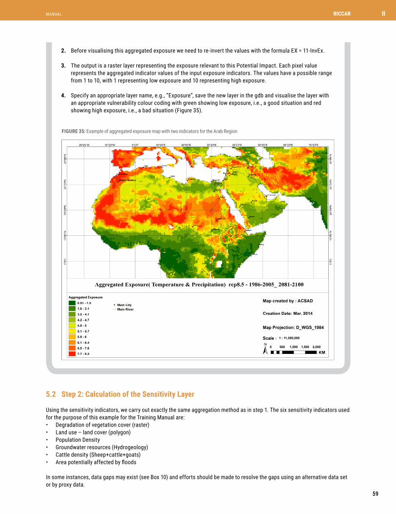
59

MANUAL

59

II

2. Before visualising this aggregated exposure we need to re-invert the values with the formula Ex = 11-InvEx.

3. The output is a raster layer representing the exposure relevant to this Potential Impact. Each pixel value represents the aggregated indicator values of the input exposure indicators. The values have a possible range from 1 to 10, with 1 representing low exposure and 10 representing high exposure.

4. Specify an appropriate layer name, e.g., “Exposure”, save the new layer in the gdb and visualise the layer with an appropriate vulnerability colour coding with green showing low exposure, i.e., a good situation and red showing high exposure, i.e., a bad situation (Figure 35).

FIGURE 35: Example of aggregated exposure map with two indicators for the Arab Region


70

Figure 35: Example of aggregated exposure map with two indicators for the Arab Region

5.2. Step 2: Calculation of the Sensitivity Layer

Using the sensitivity indicators, we carry out exactly the same aggregation method as in step 1. The six sensitivity indicators used for the purpose of this example for the Training Manual are:

• Degradation of vegetation cover (raster)

• Land Use Land Cover (polygon)

• Population Density

• Groundwater resources (Hydrogeology)

• Cattle density (Sheep+cattle+goats)

• Area potentially affected by floods

Using the sensitivity indicators, we carry out exactly the same aggregation method as in step 1. The six sensitivity indicators used for the purpose of this example for the Training Manual are:• Degradation of vegetation cover (raster)• Land use – land cover (polygon)• Population Density• Groundwater resources (Hydrogeology)• Cattle density (Sheep+cattle+goats)• Area potentially affected by floods

In some instances, data gaps may exist (see Box 10) and efforts should be made to resolve the gaps using an alternative data set or by proxy data.

5.2 Step 2: Calculation of the Sensitivity Layer

60


60

II

Practical example:

1. Open ArcToolbox and navigate to Spatial Analyst > Map Algebra. Open the tool “Raster Calculator” and enter the following expression: InvSE = Power ((11-"Reclass_PopulationDensity")*(11-"Reclass_Degradation")*(11-"Reclass_ CattleDensity")*(11-"Reclassify_AreaPotentialyEffectedbyFlood")*(11-"Reclass_HydrogeologicalUnits")*(11- "Reclass_GLC1")), (1/6))

* Kindly recall that the inversion (11-x) is not necessary if expert judgement was applied at the classification stage. 1/6 represents 1 over the number of indicators included in this example.

2. Specify an output layer name, save the aggregated sensitivity layer in the gdb. Before visualising this aggregated Exposure we need to re-invert the values with the formula SE = 11-InvSE (see section 7.3 for explanation why). Visualise the newly aggregated sensitivity layer with the same vulnerability colour coding (Figure 37). The output is a raster layer representing the sensitivity relevant for PI2. For this test case the values range from 1 to 10, with 1 representing low sensitivity and 10 representing a high sensitivity.


71

Practical example:

1. Open ArcToolbox and navigate to Spatial Analyst > Map Algebra. Open the tool “Raster Calculator” and enter the following expression:

InvSE = Power ((11-"Reclass_PopulationDensity")*(11-"Reclass_Degradation")*(11-"Reclass_CattleDensity")*(11-"Reclassify_AreaPotentialyEffectedbyFlood")*(11-

"Reclass_HydrogeologicalUnits")*(11-"Reclass_GLC1")), (1/6))

* Kindly recall that the inversion (11-x) is not necessary if expert judgement was applied at the classification stage. 1/6 represents 1 over the number of indicators included in this example.

Figure 36: Example of aggregating six sensitivity indicators in the Raster Calculator

2. Specify an output layer name, save the aggregated sensitivity layer in the gdb. Before visualising this aggregated Exposure we need to re-invert the values with the formula SE = 11-InvSE (see section 7.3 for explanation why). Visualise the newly aggregated sensitivity layer with the same vulnerability colour coding (Figure 37). The output is a raster layer representing the sensitivity relevant for PI2. For this test case the values range from 1 to 10, with 1 representing low sensitivity and 10 representing a high sensitivity.

FIGURE 36: Example of aggregating six sensitivity indicators in the Raster Calculator

61

MANUAL

61

II

FIGURE 37: Example of aggregated sensitivity map with six indicators for the Arab Region


72

Figure 37. Example of aggregated sensitivity map with six indicators for the Arab Region

Box 10: Data Gaps

It should be noted that data availability remains a constraint and challenge when conducting vulnerability assessment in the Arab region. Data gaps exist at the level of indicator availability among countries in the region, and are missing for the specified time periods (e.g., years) when a data is available for a given indicator that is available in most countries. This can be particularly challenging when collecting data in some of the Arab region’s least developed countries and for the State of Palestine.

Statistical analysis and masking out certain data in GIS can be used to off-set these challenges. However, a comprehensive review that compares between proposed indicators and available datasets should be undertaken at the inception on an assessment.

BOX 10: Data Gaps

It should be noted that data availability remains a constraint and challenge when conducting vulnerability assessment in the Arab region. Data gaps exist at the level of indicator availability among countries in the region, and are missing for the specified time periods (e.g., years) when a data is available for a given indicator that is available in most countries. This can be particularly challenging when collecting data in some of the Arab region’s least developed countries and for the State of Palestine.

Statistical analysis and masking out certain data in GIS can be used to off-set these challenges. However, a comprehensive review that compares between proposed indicators and available datasets should be undertaken at the inception on an assessment.

62


62

II

Using the adaptive capacity indicators, we carry out exactly the same aggregation method as in step 1 and 2. Here however no inversion of the values takes place since high values for adaptive capacity indicators (e.g., literacy) represent a low vulnerability and are thus ordered so as to be suitable for aggregation.

Adaptive Capacity indicators used for the purpose of the examples presented in this manual are:• Gridded GDP density (raster)• Official Development Aid (ODA) index

5.3 Step 3: Calculation of the Adaptive Capacity Layer

Practical example:

Open ArcToolbox and navigate to Spatial Analyst > Map Algebra. Open the tool “Raster Calculator” and enter the following expression: AC = Power(("AC_1"*"AC_2"),(0.5))

1. The output is a raster layer represents aggregated adaptive capacity to the impact “change in available water for agriculture/crops”.

2. The values range from 1 to 10, with 1 representing a low adaptive capacity and 10 representing a high adaptive capacity.

3. Specify an output layer name, save the aggregated adaptive capacity layer in the gdb and visualise the layer with the appropriate vulnerability colour coding.

FIGURE 38: Example of aggregated adaptive capacity map with two indicators for the Arab Region


73

5.3. Step 3: Calculation of the Adaptive Capacity Layer

Using the adaptive capacity indicators, we carry out exactly the same aggregation method as in step 1 and 2. Here however no inversion of the values takes place since high values for adaptive capacity indicators (e.g., literacy) represent a low vulnerability and are thus ordered so as to be suitable for aggregation.

Adaptive Capacity indicators used for the purpose of the examples presented in this manual are:

• Gridded GDP density (raster)

• Official Development Aid (ODA) index

Practical example Open ArcToolbox and navigate to Spatial Analyst > Map Algebra. Open the tool “Raster Calculator” and enter the following expression:

AC = Power(("AC_1"*"AC_2"),(0.5))

1. The output is a raster layer represents aggregated adaptive capacity to the impact “change in available water for agriculture/crops”.

2. The values range from 1 to 10, with 1 representing a low adaptive capacity and 10 representing a high adaptive capacity.

3. Specify an output layer name, save the aggregated adaptive capacity layer in the gdb and visualise the layer with the appropriate vulnerability colour coding.

Figure 38: Example of aggregated adaptive capacity map with two indicators for the Arab Region

63

MANUAL

63

II

Having calculated exposure and sensitivity, we can now calculate the potential impact.

5.4 Step 4: Calculation of the Potential Impact Layer

Practical example:


InvPI = Power( ("Inv_Ex" * "Inv_SE"),0.5)

2. For visualising the output the values need to be re-inverted using the formula: PI = 11-InvPI

3. The output is a raster layer representing the Potential Impact 2. The values range from 1 to 10, with 1 representing low potential impact and 10 representing high potential impact.

FIGURE 39: Example of potential impact map for the Arab Region


74

5.4. Step 4: Calculation of the Potential Impact Layer

Having calculated exposure and sensitivity, we can now calculate the potential impact.

Practical example:


InvPI = Power( ("Inv_EX" * "Inv_SE") ,0.5)

2. For visualising the output the values need to be re-inverted using the formula PI = 11-InvPI

3. The output is a raster layer representing the Potential Impact 2. The values range from 1 to 10, with 1 representing low potential impact and 10 representing high potential impact.

Figure 39: Example of potential impact map for the Arab Region

64


64

II

In order to calculate the single Vulnerability (e.g., V1) for a sector, the Potential Impact and the Adaptive Capacity are combined.

5.5 Step 5: Calculation of Single Vulnerability

Practical example:

1. Open ArcToolbox and navigate to Spatial Analyst > Map Algebra. Open the tool “Raster Calculator” and enter the following expression: InvVsingle = Power(("Inv_PI" * "AC"),0.5)

2. To visualise the output, values need to be re-inverted using the formula V single = 11-InvV

3. The output is a raster layer representing the vulnerability relevant to the potential impact “Change in available water for agriculture/crops”. The values range from 1 to 10, with 1 representing a low vulnerability and 10 representing a high vulnerability.

FIGURE 40: Example of vulnerability map for the Arab Region


75

5.5. Step 5: Calculation of Single Vulnerability

In order to calculate the single Vulnerability (e.g., V1) for a sector, the Potential Impact and the Adaptive Capacity are combined.

Practical example:


InvVsingle = Power(("Inv_PI" * "AC"),0.5)

2. To visualise the output, values need to be re-inverted using the formula V single = 11-InvV

3. The output is a raster layer representing the vulnerability relevant to the potential impact “Change in available water for agriculture/crops”. The values range from 1 to 10, with 1 representing a low vulnerability and 10 representing a high vulnerability.

Figure 40: Example of vulnerability map for the Arab Region

65

MANUAL

65

II

Once you have calculated the single vulnerabilities, you can also calculate the overall vulnerability using the geometric aggregation method.

5.6 Step 6: Calculation of the Overall Vulnerability Map

Practical example:

1. Open ArcToolbox and navigate to Spatial Analyst > Map Algebra. Open the tool “Raster Calculator” and enter the following expression. Note that the indicator layer titles must be replaced with the actual layer names: InvVtotal = Power( ("InvV_1” * “InvV_2”),1/2)

2. To visualise the output, the values need to be re-inverted using the formula Vtotal = 11-InvVtotal

3. The output is a raster layer representing the overall vulnerability for the Arab region. The values range from 1 to 10, with 1 representing low vulnerability and 10 representing high vulnerability.

67

MANUAL

67

III

This part of the Training Manual will review the following:

• What is remotely sensed data?• How is an image file displayed?• How are images classified? • How can the accuracy of classification be assessed?

PART III: TECHNICAL GUIDANCE ON REMOTE SENSING IMAGE CLASSIFICATION

1 INTRODUCTION AND REQUIREMENTS

2 DISPLAYING AN IMAGE FILE

The following sections provide a brief excursus on the classification of remotely sensed data which could be used to generate higher resolution thematic layers from Landsat imagery.

You will be using Exelis Visual Information Solutions (ENVI) software to conduct all satellite image processing. ENVI is widely used software which allows you to perform necessary functions, from extensive digital image data support to geometric correction to creating map composition, all within an easy-to-navigate image-processing environment. The lab displays image data that has been recorded along different wavelengths as both gray scale and colour composite images.

Satellite imagery data is made of raster data structure, where each picture element (pixel) represents recorded radiation intensity measured by the remote sensing instrument. Each pixel contains n-dimensions of data where n is the number of sensors designed to sense at a particular wavelength (e.g., visible, Infrared, etc.), called channels or bands.

In the first part of the exercise, you will use a subset of a Landsat-8 image of the part of Tunisia. This image was acquired in summer 2013 and has 11 bands. Bands 8 and 9 (panchromatic and cloud bands) will not be used in this exercise, thus each pixel contains 9 different radiation intensity values (after dropping bands 8 and 9).

• To start ENVI select Start > Programs > ENVI 5

• To open an image file from ENVI main menu, go to File > Open Image File. Select the LS8_Tunisia file and click Open.

• This brings up a new window called Available Band List. Here you have a choice to display your image either in Gray Scale or RGB Colour. Click on the Gray Scale button and select band 5. Click Load Band. This will open three windows, which are collectively referred to as the Display Group. This Display Group consists of the main Display Window, the Scroll Window and the Zoom Window, which allow you to move around in the image and to magnify different areas. You can pan around the image with your cursor or zoom in or out.

68


68

III

FIGURE 41: Available band bist in ENVI 5


80

Figure 41: Available band bist in ENVI 5

• To open LS8_Tunisia image in a True-Colour (similar to what the human eyes see), go to RGB Colour in the Available Band List and select bands 4, 3 and 2 as Red, Green and Blue, respectively. Click Display #1 and select New Display. Display the colour image by clicking Load RGB.

• To open LS8_Tunisia in a False-Colour, go the RGB Colour and select bands 5, 4 and 3 as Red, Green and Blue, respectively. Click Display #2 and select New Display. Display the colour image by clicking Load RGB. Explore different RGB band combinations yourself.

7.1. Pixel Location and Values

• You can interactively see individual pixel location and values for any image by right clicking in the main Display Window and selecting Cursor Location/Value. Move your cursor over the image and see how the DN values change. Double click the image window to hide/show this function.

7.2. Linking Satellite Images

• To link two images together for comparison, click Tools > Link > Link Displays. Move with your cursor and see how are these moves are mirrored in the second display.

7.3. Z Profiles

• This is an important function as it allows you to examine the spectral signature curves of some of the dominant surface features in your image (e.g., Vegetation, Water, Urban and bare soil). Display your image as true colour, then go to Tools > Profiles > Z Profile (Spectrum). Click on a pixel with a vegetation cover. Do you know why the spectral response (curve) of the vegetation has this shape?

• To open LS8_Tunisia image in a True-Colour (similar to what the human eyes see), go to RGB Colour in the Available Band List and select bands 4, 3 and 2 as Red, Green and Blue, respectively. Click Display #1 and select New Display. Display the colour image by clicking Load RGB.

• To open LS8_Tunisia in a False-Colour, go the RGB Colour and select bands 5, 4 and 3 as Red, Green and Blue, respectively. Click Display #2 and select New Display. Display the colour image by clicking Load RGB. Explore different RGB band combinations yourself.

• You can interactively see individual pixel location and values for any image by right clicking in the main Display Window and selecting Cursor Location/Value. Move your cursor over the image and see how the DN values change. Double click the image window to hide/show this function.

• To link two images together for comparison, click Tools > Link > Link Displays. Move with your cursor and see how are these moves are mirrored in the second display.

• This is an important function as it allows you to examine the spectral signature curves of some of the dominant surface features in your image (e.g., Vegetation, Water, Urban and bare soil). Display your image as true colour, then go to Tools>Profiles>ZProfile (Spectrum). Click on a pixel with a vegetation cover. Do you know why the spectral response (curve) of the vegetation has this shape?

2.1 Pixel Location and Values

2.2 Linking Satellite Images

2.3 ZProfiles

69

MANUAL

69

III

FIGURE 42: True and false colour image


81

Figure 42: True and false colour image

8. Image Classification

In this section of the exercise, you will be introduced to basic image classification procedures. Earth remotely sensed imagery may be analysed in order to extract thematic information. The objective of image classification is to recognize and assign particular ranges of pixel values in spectral bands to the categories (classes) concerned. If the user has previous knowledge about the surface feature of the image being analysed, the classification method is termed supervised. Conversely, if the classification is done initially by computer, and later decoded (or labelled) by the user, the classification method is termed unsupervised. Image classification is an iterative process. It is almost impossible to get classification right the first time procedure is applied. To make a good map, you will have to take several steps to get from initial to intermediate to final classification results, refining the map further at each stage. In the case of supervised classification, you can revisit your training sites, refine them, or add or remove a few to see how your map improves. In the case of unsupervised classification, the number of classes and iterations can be altered. Your ultimate goal is to produce the best available land cover map, either through a supervised or unsupervised classification or a combination of the two. One of the initial duties in image classification is to decide on final classes to be used. This is different for each location and final application of the map. For example, in Boston you may choose more than 10 classes where a great deal of variety is to be found. In the Great Sahara, there may only 2 classes (sandy or rocky fields).

8.1. Unsupervised Classification

Unsupervised classification is an exploratory procedure, in which classes are determined by a classification algorithm, without the user's help. Newly generated computer (or spectral) classes are then labelled by the user, who possesses foreknowledge of the landscape in question. Unsupervised classification is useful if the remote sensing analyst (you) cannot easily discern if a class is pure or mixed. It can also be used as a preliminary step in refining knowledge of the spectral classes present in the image so that subsequent supervised classification can be carried out more efficiently. In this case, classes identified by unsupervised analysis can be used as a basis to select training samples (sites) to be used during the supervised classification procedure.

Unsupervised classification technique initially requires that the number of spectral classes be given. This number may be obtained in different ways. A common approach is to allow around 2 spectral classes per land cover category. For example, for 15 different land cover classes, (e.g., trees, grass,

Unsupervised classification is an exploratory procedure, in which classes are determined by a classification algorithm, without the user's help. Newly generated computer (or spectral) classes are then labelled by the user, who possesses foreknowledge of the landscape in question. Unsupervised classification is useful if the remote sensing analyst (you) cannot easily discern if a class is pure or mixed. It can also be used as a preliminary step in refining knowledge of the spectral classes present in the image so that subsequent supervised classification can be carried out more efficiently. In this case, classes identified by unsupervised analysis can be used as a basis to select training samples (sites) to be used during the supervised classification procedure.

Unsupervised classification technique initially requires that the number of spectral classes be given. This number may be obtained in different ways. A common approach is to allow around 2 spectral classes per land cover category. For example, for 15 different land cover classes, (e.g., trees, grass, wetland, urban high, urban low, bare-soil, water etc.) you would assign 30 initial spectral classes to be identified with the unsupervised classification procedure! However, this would be very computer intensive. Thus, for this exercise section, you will use 10 classes to practice the procedure.

3.1 UnsupervisedClassification

3 IMAGE CLASSIFICATION In this section of the exercise, you will be introduced to basic image classification procedures. Earth remotely sensed imagery may be analysed in order to extract thematic information. The objective of image classification is to recognize and assign particular ranges of pixel values in spectral bands to the categories (classes) concerned. If the user has previous knowledge about the surface feature of the image being analysed, the classification method is termed supervised. Conversely, if the classification is done initially by computer, and later decoded (or labelled) by the user, the classification method is termed unsupervised.

Image classification is an iterative process. It is almost impossible to get classification right the first time procedure is applied. To make a good map, you will have to take several steps to get from initial to intermediate to final classification results, refining the map further at each stage. In the case of supervised classification, you can revisit your training sites, refine them, or add or remove a few to see how your map improves. In the case of unsupervised classification, the number of classes and iterations can be altered. Your ultimate goal is to produce the best available land cover map, either through a supervised or unsupervised classification or a combination of the two. One of the initial duties in image classification is to decide on final classes to be used. This is different for each location and final application of the map. For example, in Boston you may choose more than 10 classes where a great deal of variety is to be found. In the Great Sahara, there may only 2 classes (sandy or rocky fields).

70


70

III

• A small subset of the LS8_Tunisia will be used for classification. To generate a small subset from the raw image go to Basic Tools > Resize Data (Spatial/Spectral) and select LS8_Tunisia image. Click on Spatial Subset > ROI/EVF and select clip_box1.evf file. Select EVF:clip and hit OK (evf is an ENVI vector file format that contains a large polygon that will be used for clipping). Click OK. Name the output file sub_Tunisia. Display sub_Tunisia in true colour. Navigate to the image and try to familiarise yourself with land cover/use types in the area.

• To conduct an unsupervised classification on sub_Tunisia image go to Classification>Unsupervised>K-means. The K-Means procedure calculates initial class means randomly in the data space and then iteratively clusters the pixels into the nearest class using a minimum distance technique. Each iteration recalculates class means and reclassifies pixels with respect to the new means. All pixels are classified to the nearest class unless a standard deviation or distance threshold is specified, in which case some pixels may be unclassified if they do not meet the selected criteria. This process continues until the number of pixels in each class changes by less than the selected pixel change threshold or the maximum number of iterations is reached. Select sub_Tunisia image to be classified and hit OK.

• In the K-Means Parameters dialog window, first enter 10 as a desired number of classes. Enter a threshold value of 5. This value can be changed later in your other attempts. Choose 20 for Maximum Number of Iterations. Accept default (keep blank) for other options. Name the Output File sub_Tunisia_unsup10 and click OK.

• This process will take a few minutes. Once the process is completed you will get a spectral class map with the number of classes, initially requested (10 classes). Use the Link function (Tools > Link > Display Link) to compare between the derived unsupervised image (sub_Tunisia_unsup10) and the original image (sub_Tunisia).

• To display the spectral classes determined by the computer, go to Tools > Colour Mapping > Class Colour Mapping. Now your goal is to identify in the classified image which spectral class belongs to which land cover class. Label each class with a suitable name. Our goal is to extract at least five land use – land cover classes which can be as follows: - Water (including ocean, lakes and rivers) - Agricultural lands (croplands) - Forest (deciduae and evergreen) - Bare ground (desert sand and bed rock) - Urban (residential and industrial areas as well as major roads network) Most likely there will be several spectral classes that represent the same land cover type. If this is the case, then you are advised to give all classes which represent the same cover type the same name, but with different numbers (e.g., water1, water2, water3; urban1, urban2, etc.). Give each type of the land use – land cover a meaningful colour (e.g., provide a blue colour to the water1, water2 and water3 classes and green colour to the urban1 and urban2 classes, etc.). Save frequently from Options > Save Changes.

Supervised classification uses a set of user-defined spectral signatures to classify an image. The spectral signatures are derived from training sets that are created by interactively digitising features of interest on an image. Care must be taken to create effective training signature sets. Important points to keep in mind include: 1) Each training site should appear homogenous; 2) Delineate several training sites within each information class; 3) If the same information class appears different in two or more locations (e.g., sunny vs. shady locations), consider collecting separate training sites for each class and then combine them later.

• The first step in supervised classification is to start collecting the training sites (ROIs). Go to Overlay > Region of Interest and draw your training samples in the form of closed polygons (For this exercise a minimum of 15 polygons per class is required). Click the left mouse button in the Zoom window to establish the first point of the ROI polygon. Select further border points in sequence by clicking the left button again, and close the polygon by clicking the right mouse button. The middle mouse button deletes the most recent point, or (if you have closed the polygon) the entire polygon. Try using Google Earth to acquaint yourself with the different land-cover types in the image. Once you collect all of the polygons you are interested in save the ROIs file (File > Save ROIs) and name it roi_supervised.

• To perform the supervised classification, go to Classification>Supervised>MaximumLikelihood. In the Classification input file, select sub_Tunisia and click OK. Note that if there are no available training regions already loaded, the Maximum Likelihood method will not work. That is, if you come back to classify an image at any time other than the time when you generate and save your ROIs, you will first have to load the ROIs on the image then run the classification.

3.2 SupervisedClassification

71

MANUAL

71

III

• Select all regions of interest (ROIs) as the training classes. Set Probability Threshold to None. Name the final classified image Sub_Tunisia_super. Check NO for Output Rule Images then press OK to begin classification. Display your classified image as a single band. Take a look at your image. Are locations that you are most familiar with classified correctly?

FIGURE 43: Supervised classification map (Maximum Likelihood Approach)


83

• The first step in supervised classification is to start collecting the training sites (ROIs). Go to Overlay > Region of Interest and draw your training samples in the form of closed polygons (For this exercise a minimum of 15 polygons per class is required). Click the left mouse button in the Zoom window to establish the first point of the ROI polygon. Select further border points in sequence by clicking the left button again, and close the polygon by clicking the right mouse button. The middle mouse button deletes the most recent point, or (if you have closed the polygon) the entire polygon. Try using Google Earth to acquaint yourself with the different land-cover types in the image. Once you collect all of the polygons you are interested in save the ROIs file (File > Save ROIs) and name it roi_supervised.

• To perform the supervised classification, go to Classification > Supervised > Maximum Likelihood. In the Classification input file, select sub_Tunisia and click OK. Note that if there are no available training regions already loaded, the Maximum Likelihood method will not work. That is, if you come back to classify an image at any time other than the time when you generate and save your ROIs, you will first have to load the ROIs on the image then run the classification.

• Select all regions of interest (ROIs) as the training classes. Set Probability Threshold to None. Name the final classified image Sub_Tunisia_super. Check NO for Output Rule Images then press OK to begin classification. Display your classified image as a single band. Take a look at your image. Are locations that you are most familiar with classified correctly?

Figure 43: Supervised classification map (Maximum Likelihood Approach)

4 POST CLASSIFICATION AND ACCURACY ASSESSMENT

To add a map legend and scale bar, open the classified image (Sub_Tunisia_super) and go to Overlay > Annotation. In the Scroll Window, position the red box at the left corner of the classified image and click on Object > Map Key. Click once with the left mouse button in the Display Window to place the Map Key in the image. Click and drag the Map Key using the left mouse button in the display to place the key. Change the Colour of the text to Black and the colour of the Background to White. Now, click on Edit Map Key Items, select the Unclassified class then click the Delete Item icon and press OK. Over the map legend, click on the right mouse button to make the position of the Map Key permanent. Now add a scale bar to the map from Object > Scale Bar. Take a screenshot of the classified image with the added annotation.

4.1 Map Annotation

72


72

III

In this step you will convert one of the derived classes (e.g., the water body) from raster to vector, which can be overlaid on your original colour composite image or uploaded to ArcGIS software as shapefile. Go to Classification>PostClassification>ClassificationtoVector. Select your classified image (Sub_Tunisia_super) and press OK. Select the water body class under Select Classes to Vectorise. Name the Output File water and hit OK. In the Available Vectors List window select the derived-vector file and click Load Selected. Select Display # 1 (where your original image is displayed as RGB) and click OK. The vector appears in the image window. You can change the colour of the vector layer from Current Layer (for example, change from white to blue colour) and click Apply. Navigate the image with the water body overlaid.

In this section of the lab you will check how accurate your classification map is (Sub_Tunisia_super). In order to calculate the accuracy report you need to create the second set of ROIs (recall the supervised classification section), which will be used to verify your classification accuracy. Name the new output file ROIs_points.

Now you are ready to calculate the Accuracy Assessment on the final classified image. In this step you will be generating a Confusion Matrix from which the accuracy of your classification can be assessed.

To generate a confusion matrix, go to Classification>PostClassification>ConfusionMatrix. First choose your image and press OK. Then in Match Class Parameters dialog, choose the Ground Truth ROIs you created for validation (the ROIs_points file) and select the corresponding classes from the Classified Image. Choose both Pixels and Percent, Yes for Report Accuracy Assessment and press OK. Save your resulting report as an ASCII file and name it accuracy_report. Please note, if your total accuracy is less than 85%, you have to refine your training sites and repeat the classification one more time.

4.2 ExportingClassestoVectorLayers/Shapefiles

4.3 ClassificationAccuracyAssessment

MANUAL

7373

ENDNOTES

1. The Arab region is defined as the area encompassing the 22 members of the League of Arab States, namely Algeria, Bahrain, Comoros, Djibouti, Egypt, Iraq, Jordan, Kuwait, Lebanon, Libya, Mauritania, Morocco, Oman, State of Palestine, Qatar, Saudi Arabia, Somalia, Sudan, Syrian Arab Republic, Tunisia, United Arab Emirates and Yemen.

2. Arab Ministerial Declaration on Climate Change, Council of Arab Ministers Responsible for the Environment (CAMRE), League of Arab States, Cairo, 6 December 2007.

3. More information is available on the RICCAR website (www.riccar.org).

4. Climate Change 2007: Impacts, Adaptation and Vulnerability. Contribution of Working Group II to the Fourth Assessment Report of the Intergovernmental Panel on Climate Change, M.L. Parry, O.F. Canziani, J.P. Palutikof, P.J. van der Linden and C.E. Hanson, Eds., Cambridge University Press, Cambridge, UK, 717-743 (Appendix I. Glossary).

5. See “Special Issue of the Climatic Change Journal on the Framework for the Development of New Socioeconomic Scenarios for Climate Change Research”, available at: https://www2.cgd.ucar.edu/research/iconics/publications/ssps. Members of the Integrated Assessment Modelling (IAM) and Impacts, Adaptation and Vulnerability (IAV) research communities formed an International Committee on New Integrated Climate Change Assessment Scenarios to coordinate a range of activities contributing to the Parallel Phase of the New Scenarios Process. The Committee is organized into Working Groups dealing with specific topics focused on the development of the SSPs, which can be used in conjunction with the RCPs to develop scenarios for use by the research community, available at: https://www2.cgd.ucar.edu/research/iconics.

6. Narratives (storylines) are qualitative descriptions of the relationships among different trends and socio-economic developments assumed in a scenario.

7. The workshop brought together members of the Integrated Assessment Modelling (IAM), Impacts, Adaptation and Vulnerability (IAV), and Climate Modelling (CM) communities, led to the adoption of a unified framework for the development of a small set of SSPs, to be used in conjunction with the Regional Concentration Pathways (RCPs) and associated climate model simulations for the development and assessment of integrated research. See O’Neill, B.C., Carter, T.R., Ebi, K.L., Edmonds, J., Hallegatte, S., Kemp-Benedict, E., Kriegler, E., Mearns, L., Moss, R., Riahi, K., van Ruijven, B., van Vuuren, D. 2012. "Meeting Report of the Workshop on The Nature and Use of New Socioeconomic Pathways for Climate Change Research," Boulder, CO, November 2-4, 2011. Available at: http://www.isp.ucar.edu/socioeconomic-pathways.

8. Population and urbanization scenarios were developed by the International Institute for Applied Systems Analysis (IIASA) and the National Center for Atmospheric Research (NCAR).

9. The GDP projections are based on harmonized assumptions for the interpretation of the SSP storylines in terms of the main drivers of economic growth.

10. The Vulnerability Sourcebook (GIZ, 2014) provides a comprehensive description of how impact chains are developed and indicators derived from them in Modules 2 and 3.

11. Adapted from CIDA, 2004, reprinted in AFB, 2010, as cited in GIZ, 2011.

12. The Arab Domain is also referred to as the MENA Domain in CORDEx and the Earth System Grid Federation (ESGF). It is also noted that Comoros, while an Arab State, is not included in the Arab Domain given its geographic location. Comoros can be otherwise be studied using high-resolution global climate models or the regional climate modelling domain covering the African region.

13. Note that by applying the formula Integer {10*(Log(xi )-(-0.7))/(6.3–(-0.7))} +1, to the values of the original data series (except for the maximum value which by default will get the value 10) the classes can be obtained directly.

14. The importance of expert choices was made clear in 6.2 and 6.3 in the practical examples presented for the two other methods of data evaluation: Evaluation of Indicators Using a Reference, and Evaluating Indicators Based on Expert Opinion.

15. As global minima often appeared to include a country of the region, the adjustment was made for the maximum values by taking the average of the 3 highest countries at the global level to dampen the impact of potential global outliers.

16. See http://webhelp.esri.com/ for the different classification methods.

17. While the summation and multiplication approaches result in a quantitative index score, multicriteria analysis methods use nonlinear aggregation methods that generate index ranks instead of scores. For an overview of these methods see OECD (2008).

18. An exception is the use of an arithmetic aggregation for the calculation of some sub-indices in the Adaptive Capacity dimension.

19. Other methods are the benefit of the doubt (BOD) approach, the unobserved components model (UCM), and the conjoint analysis (CA). For a more complete overview of weighting methods see OECD (2008).

20. In the cases where global minima and maxima have been used in the normalization formula leading to an evaluation over 8 classes, the inversion formula used is 9 – x.

21. For all aggregation steps, indicator, dimension, or component inversion might be necessary, see 7.3: Preparing Indicator Values for Aggregation. For ease of exposition the following aggregation formulas are assumed to apply after the appropriate inversions have been done.

22. Some socio-economic determinants of adaptive capacity are generic (e.g., education, income and health), i.e., they enable adaptation across the localities and countries irrespective of their location and climate impacts, while other determinants are more specific to particular climate change impacts such as floods or droughts.

MANUAL

74


23. However a geometric aggregation can also be applied if you decide that this better matches the characteristics of your data. In this case, the formula for this aggregation step would be:

Sub-Ind ACi = (AC1 * AC2 * AC3 * … * ACn)1/n in the case of equal weights; and

Sub-Ind ACi

= (AC1)w1 * (AC2)

w2 * (AC3)w3 * … * (ACn)wn in the case of a weighted geometric aggregation.

24. Note that the aggregation of the Infrastructure dimension includes a supplementary level of aggregation: indicators and sub-indices are first combined to calculate a composite index for each of the five pillars of this dimension: energy, transport, health, water and sanitation supply, and environment. These are then aggregated to calculate the index of the Infrastructure dimension.

25. This remark is also valid for the weighting choices made at other steps of the aggregation process.

26. The net impact of the variations of adaptive capacity and potential impact depends on if we are considering an area with low or high starting levels of adaptive capacity and potential impact, as the influence of the partial compensability property of the geometric aggregation should also be considered, see paragraph 7.2.

27. General tutorials for working with ArcGIS can be found at: http://help.arcgis.com/en/arcgisdesktop/10.0/help/index.html#//00v20000000t000000.htm.

75

MANUAL

REFERENCES

Adelphi, 2013. Methodology for an Integrated Vulnerability Assessment of the Arab Region, PowerPoint presentation delivered by K. Fritzsche (adelphi) at Fifth RICCAR Expert Group Meeting, Amman, 11-12 December 2013. Available a: https://www.unescwa.org/events/fifth-expert-group-meeting-regional-initiative-assessment-impact-climate-change-water

ESCWA et al., 2017. Arab Climate Change Assessment Report – Main Report. Beirut, E/ESCWA/SDPD/2017/RICCAR/Report. Available at www.riccar.org. Füssel H. and Klein R., 2006. Climate change vulnerability assessments: an evolution of conceptual thinking. Climatic Change 75 (3), pp. 301–329.

GIZ, 2011. Making Adaptation Count - Concepts and Options for Monitoring and Evaluation of Climate Change Adaptation. Published by Federal Ministry for Economic Cooperation and Development (BMZ). Eschborn, August 2011.

GIZ, 2014. The Vulnerability Sourcebook. Concepts and Guidelines for Standardised Vulnerability Assessments. Online available at: http://star-www.giz.de/pub?r=37621&lang=1

Hinkel, J. 2011. Indicators of vulnerability and adaptive capacity: Towards a clarification of the science–policy interface. Global Environmental Change 21, pp.198–208. IPCC, 2001. Annex B: Glossary of Terms. In: Watson, R.T. and the Core Writing Team (ed.) 2001: Climate Change 2001: Synthesis Report (Contribution of Working Groups I, II and III to the Third Assessment Report of the Intergovernmental Panel on Climate Change). Cambridge University Press, Cambridge UK, New York, USA, pp. 365–389.

IPCC, 2007. Contribution of Working Group II to the Fourth Assessment Report of the Intergovernmental Panel on Climate Change, 2007, M.L. Parry, O.F. Canziani, J.P. Palutikof, P.J. van der Linden and C.E. Hanson (eds), Cambridge University Press, Cambridge, United Kingdom and New York, NY, USA. Available at: https://www.ipcc.ch/publications_and_data/ar4/wg2/en/contents.html

IPCC, 2014. Annex II: Glossary [Agard, J., E.L.F. Schipper, J. Birkmann, M. Campos, C. Dubeux, Y. Nojiri, L. Olsson, B. Osman-Elasha, M. Pelling, M.J. Prather, M.G. Rivera-Ferre, O.C. Ruppel, A. Sallenger, K.R. Smith, A.L. St. Clair, K.J. Mach, M.D. Mastrandrea, and T.E. Bilir (eds.)]. In: Climate Change 2014: Impacts, Adaptation, and Vulnerability. Part B: Regional Aspects. Contribution of Working Group II to the Fifth Assessment Report of the Intergovernmental Panel on Climate Change [Barros, V.R., C.B. Field, D.J. Dokken, M.D. Mastrandrea, K.J. Mach, T.E. Bilir, M. Chatterjee, K.L. Ebi, Y.O. Estrada, R.C. Genova, B. Girma, E.S. Kissel, A.N. Levy, S. MacCracken, P.R. Mastrandrea, and L.L. White (eds.)]. Cambridge University Press, Cambridge, United Kingdom and New York, NY, USA, pp. 1757-1776. Available at: http://www.ipcc.ch/pdf/assessment-report/ar5/wg2/WGIIAR5-AnnexII_FINAL.pdf

Karoui, H., 2006. Global Trends in Gulf and Middle East Population Evolution. Middle East Studies Online Journal. Available at http://www.middle-east-studies.net/?p=1756 (accessed 31 October 2013).

Kienberger, S., Blaschke, T., Zaidi. R.Z., 2012. A framework for spatio-temporal scales and concepts from different disciplines: the 'vulnerability cube. Natural Hazards. Available at: http://dx.doi.org/ 10.1007/s11069-012-0513-x

Klugman, J., Rodríguez, F., Choi, H.-J., 2011. The HDI 2010: New Controversies, Old Critiques. Available at: http://hdr.undp.org/sites/default/files/hdrp_2011_01.pdf (accessed 17 April 2014).

Nakicenovic, N. et al (2000). Special Report on Emissions Scenarios: A Special Report of Working Group III of the Intergovernmental Panel on Climate Change, Cambridge University Press, Cambridge, U.K., 599 pp. Available at: http://www.grida.no/climate/ipcc/emission/index.htm

OECD, 2008. Handbook on Constructing Composite Indicators. Methodology and User Guide. Available at: http://www.oecd.org/std/42495745.pdf (accessed 4 April 2014).

Schneiderbauer, S., 2013. “General background and concepts of vulnerability assessment.” Powerpoint presentation at the 1st Meeting of the Vulnerability Assessment Working Group, 29 January 2013, Beirut, Lebanon.

Schneiderbauer, S., Pedoth, L., Zhang, D., Zebisch, M., 2011. “Assessing adaptive capacity within regional climate change vulnerability studies – an Alpine example,” Natural Hazards, pp. 1-15.

UN-Habitat, 2006. The State of the World s Cities 2004/2005: Globalization and Urban Culture. Available at: http://ww2.unhabitat.org/mediacentre/sowckit.asp (accessed 7 November 2013).

UN-Habitat, 2012. The State of Arab Cities, 2012: The Challenge of Urban Transition. Second edition. Available at: https://unhabitat.org/books/the-state-of-arab-cities-2012-challenges-of-urban-transition/ (accessed 20 May 2015).

UNEP, 2010. Environment Outlook for the Arab Region. Environment for Development and Human Well-being. Available at: http://eoar.cedare.int/report/EOAR_Full%20Report%20%28EN%29.pdf (accessed 7 November 2013).

training manual on the integrated vulnerability assessment

Documents