1

TRAJECTORY DESIGN FOR THE TRANSITING EXOPLANET SURVEY SATELLITE

Donald J. Dichmann(1), Joel J.K. Parker(2), Trevor W. Williams(3), Chad R. Mendelsohn(4) (1,2,3,4)Code 595.0, NASA Goddard Space Flight Center, 8800 Greenbelt Road, Greenbelt MD 20771. 301-286-6621. donald.j.dichmann@nasa.gov

Abstract: The Transiting Exoplanet Survey Satellite (TESS) is a National Aeronautics and Space Administration (NASA) mission, scheduled to be launched in 2017. TESS will travel in a highly eccentric orbit around Earth, with initial perigee radius near 17 Earth radii (Re) and apogee radius near 59 Re. The orbit period is near 2:1 resonance with the Moon, with apogee nearly 90 degrees out-of-phase with the Moon, in a configuration that has been shown to be operationally stable. TESS will execute phasing loops followed by a lunar flyby, with a final maneuver to achieve 2:1 resonance with the Moon. The goals of a resonant orbit with long-term stability, short eclipses and limited oscillations of perigee present significant challenges to the trajectory design. To rapidly assess launch opportunities, we adapted the Schematics Window Methodology (SWM76) launch window analysis tool to assess the TESS mission constraints. To understand the long-term dynamics of such a resonant orbit in the Earth-Moon system we employed Dynamical Systems Theory in the Circular Restricted 3-Body Problem (CR3BP). For precise trajectory analysis we use a high-fidelity model and multiple shooting in the General Mission Analysis Tool (GMAT) to optimize the maneuver delta-V and meet mission constraints. Finally we describe how the techniques we have developed can be applied to missions with similar requirements. Keywords: resonant orbit, stability, lunar flyby, phasing loops, trajectory optimization 1. Introduction The Transiting Exoplanet Survey Satellite (TESS), scheduled to be launched in 2017, is a NASA Explorer-class mission that will perform a survey of the entire sky over its nominal two-year mission. TESS will monitor 500,000 stars for temporary drops in brightness caused by planetary transits, and discover thousands of exoplanets in orbit around the brightest stars in the sky. This first-ever spaceborne all-sky transit survey will identify planets ranging from Earth-sized to gas giants, around a wide range of stellar types and orbital distances. TESS will provide prime targets for observation with the James Webb Space Telescope, as well as other large ground-based and space-based telescopes of the future [1]. TESS will travel in a highly eccentric orbit around Earth, with initial perigee radius near 17 Earth radii (Re) and apogee radius near 59 Re. The high apogee, close to Moon orbit radius, allows observations far from Earth for extended intervals, while the perigee much closer to Earth allows science data downlink at a high data rate. An orbit period near 2:1 resonance with the Moon, with each apogee nearly 90 degrees out-of-phase with the Moon, has been shown to be operationally stable. The trajectory sequence for TESS is illustrated in a timeline in Figure 1 and an orbit diagram in Figure 2. The orbit design draws from analysis by Mathews et al. [2] and McGiffin et al. [3]. TESS will execute 3.5 phasing orbits followed by a lunar flyby. The flyby accomplishes several mission goals. It places TESS in a Transfer orbit with perigee radius equal to the Science orbit perigee radius near 17 Re. The flyby also achieves the line of apsides and inclination to the ecliptic plane designed to minimize eclipses.

https://ntrs.nasa.gov/search.jsp?R=20140007518 2018-07-19T11:25:31+00:00Z

2

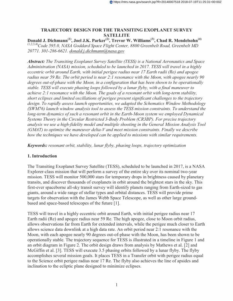
Figure 1. TESS mission timeline. There are three phasing loops, followed by a Translunar Injection maneuver that sends the spacecraft to a lunar flyby. The flyby raises perigee to mission altitude. At the next perigee, a Period Adjust Maneuver (PAM) is performed to place TESS in a 2:1 resonant orbit with the Moon.

Finally, the radius of the Transfer orbit at Post-Lunar Encounter Apogee (PLEA) near 81 Re is set to achieve an important trajectory goal for the Time of Flight (TOF) to the next perigee, called Post-Lunar Encounter Perigee (PLEP). When TESS reaches PLEP, the Moon-Earth-Vehicle angle will be less than 30 deg. At PLEP, the PAM burn is performed at perigee to achieve 2:1 resonance with the Moon. The resonant orbit, together with the alignment condition at PLEP, achieves the Lunar Resonant Phasing (LRP) condition that assures operational stability. Ideally the Moon-Earth-Vehicle angle at PLEP would be 0 deg, but that is neither practical nor necessary. Analysis and simulations show that a PLEP misalignment angle no greater than 30 deg is sufficient. Because TESS is in 2:1 resonance with the Moon, one half orbit period that it takes TESS to travel between perigee and apogee equals one-quarter orbit period for the Moon. So while TESS moves through 180 deg of true anomaly between perigee and apogee, the Moon moves through about 90 deg of true anomaly1. Consequently at the next apogee, and at subsequent apogees, the Moon-Earth-Vehicle angle will be 90 deg. At each perigee, the Moon-Earth-Vehicle will be 0 deg or 180 deg. As a result of the LRP condition, the TESS spacecraft remains far from the Moon during its Science orbit, despite the high apogee, and the orbit remains operationally stable for the duration of the mission. The LRP condition can be visualized most easily the Earth-Moon rotating frame, where the Earth-Moon direction defines the x axis and the Moon orbit normal defines the z axis. The LRP condition can be seen in Figure 5 for an idealized periodic orbit in the CR3BP, and for a realistic TESS orbit in Figure 9(b). For such a highly eccentric orbit it is known that eccentricity and inclination oscillate together, as described by the Kozai mechanism discussed in Section 3.3. The Science orbit, also called

1 The exact angle the Moon travel during a TESS half-orbit will differ from 90 deg. The Moon’s orbit has an eccentricity of 0.0549. Due to Sun perturbations, the Moon does not move on a Keplerian orbit. Finally, the TESS orbit will not be exactly resonant. Instead the orbit period will oscillate around the resonant period.

3

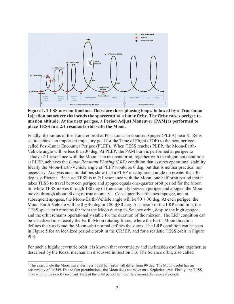
Mission orbit, must keep perigee below 22 Re to maintain communications and above 7 Re to reduce risk of collision within the geosynchronous belt.

Figure 2. Diagram of the trajectory events [1]. The Translunar Injection (TLI) segment (green) sends the spacecraft to lunar flyby. Following flyby, TESS travels on the Transfer orbit (blue) that delivers it to the Science orbit (black).

The goals to achieve a resonant orbit with long-term orbit stability, short eclipses and limited oscillations of perigee, together with the need for a lunar flyby, present significant challenges to the trajectory design. This paper describes the flight dynamics analysis performed to date for TESS at NASA Goddard Space Flight Center. The paper is organized as follows. In Section 2 we describe the rapid assessment of launch opportunities using the Schematic Window Methodology (SWM76) launch window tool, developed originally for the Magnetospheric Multiscale (MMS) mission. Computational speed in SWM76 is achieved by making use of the orbital Variation of Parameter (VOP) equations, together with “geometry proxies” for the constraints. Geometry proxies were derived for three TESS orbital constraints: (1) eclipses are limited in duration; (2) the Science orbit can be reachable via a lunar gravity-assist, and (3) TESS achieves the LRP condition. During the spacecraft design, one critical design parameter has been the number of batteries to carry, which determines the number of hours of eclipse that TESS can handle. SWM76 allowed us to rapidly compare the achievable launch opportunities where the maximum eclipse is constrained to 2, 4 or 6 hours. The operational stability of a resonant orbit with the LRP condition is a central feature for mission design. This fact has been demonstrated by the IBEX mission [4], [5]: It limits the variability of orbit elements, improves long-term predictability, and eliminates the need for orbit maintenance maneuvers. In Section 3, we show how Dynamical Systems Theory was used to examine the long-term dynamics in the Earth-Moon system using a Circular Restricted 3-Body model. In particular, Gangestad et al. [6] showed how the Kozai mechanism for highly eccentric orbits can be used to design a Science orbit that achieves the Mission goals. Because the Sun’s

4

gravitation has a significant effect on the dynamics, we extended the analysis to a Bi-circular Restricted 4-Body model. For more precise trajectory analysis we use a high-fidelity ephemeris model in GMAT. In Section 4 we describe the features of GMAT. To initialize the trajectory design in GMAT we develop two-body and three-body approximations of the trajectory segments. We then show how multiple shooting in GMAT was employed to meet the mission constraints are met, building on the two-body and three-body analysis in [6]. In Section 5 we discuss how the flight dynamics analysis techniques we have developed for TESS can be applied to science missions with similar requirements, and in Section 6 we summarize the our conclusions. 2. Launch Opportunity Assessment using SWM76 SWM76 is a launch window tool that was developed [7] for the NASA MMS mission, which will fly four spacecraft in formation in a highly eccentric orbit to study magnetic reconnection in the magnetosphere of the Earth. SWM76 uses the VOP equations [8] as the basis for a semi-analytic quantification of the dominant oblateness and lunisolar perturbation effects on the MMS orbit. Instead of applying a full force model over successive, necessarily short, time steps, this approach averages the effects of the relatively small perturbations over a complete MMS orbit and then applies these lunisolar and oblateness corrections to the orbital elements. The result is an accurate approximation to the perturbed MMS orbit, but obtained with much greater computational efficiency. In fact, this approach, coupled with an interpretation of the MMS science and engineering constraints in terms of geometry proxies (e.g. solar latitude used as a proxy for eclipse durations), allows a scan through all possible Right Ascension of the Ascending Node (RAAN) and Argument of Periapsis (AOP) values between 0 and 360 deg for a given launch date, in 2 deg steps, to be carried out in less than 10 s on a typical modern laptop. By comparison, evaluating a single one of these 1802 = 32,400 (RAAN, AOP) pairs using the much more detailed MMS End-to-End (ETE) simulation code, which uses full force model numerical propagation, and includes formation maneuvers with navigation and execution errors, etc., takes 6 to 8 hours. SWM76 has therefore proved to be a valuable adjunct to the ETE code, allowing good launch RAAN and AOP values to be generated for use by the latter. It should be noted that good agreement has been observed between the predictions of SWM76 and the results generated by the ETE code. The results produced by SWM76 are in graphical form: they show the regions in the (RAAN, AOP)-plane over which each of the MMS orbital constraints is satisfied. The launch window (if any exists) for this date is then the intersection of these regions. This graphical output form has proved to be very useful for providing insight into which constraints are most onerous, and so could be most profitable to relax, allowing launches to be possible on a wider range of dates. SWM76 also provides additional outputs, such as the minimum perigee altitude reached during the mission: this is a result of lunisolar perturbations, and is a strong function of RAAN, AOP and launch date. Knowledge of the minimum perigee altitude is useful for predicting the amount of fuel that MMS will require for orbit maintenance: this is an important question, given the extensive maneuvering that MMS must carry out.

5

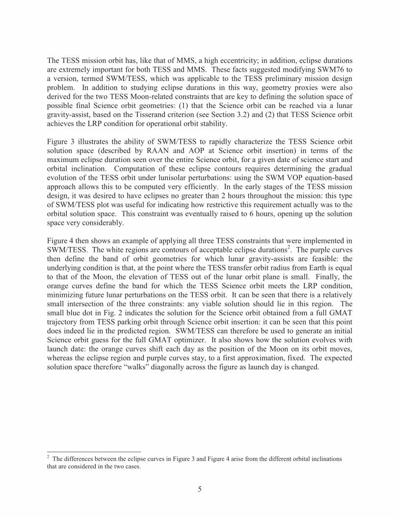
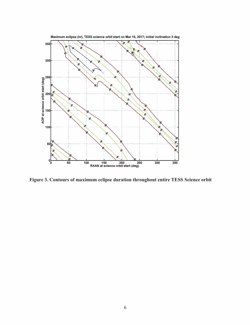
The TESS mission orbit has, like that of MMS, a high eccentricity; in addition, eclipse durations are extremely important for both TESS and MMS. These facts suggested modifying SWM76 to a version, termed SWM/TESS, which was applicable to the TESS preliminary mission design problem. In addition to studying eclipse durations in this way, geometry proxies were also derived for the two TESS Moon-related constraints that are key to defining the solution space of possible final Science orbit geometries: (1) that the Science orbit can be reached via a lunar gravity-assist, based on the Tisserand criterion (see Section 3.2) and (2) that TESS Science orbit achieves the LRP condition for operational orbit stability. Figure 3 illustrates the ability of SWM/TESS to rapidly characterize the TESS Science orbit solution space (described by RAAN and AOP at Science orbit insertion) in terms of the maximum eclipse duration seen over the entire Science orbit, for a given date of science start and orbital inclination. Computation of these eclipse contours requires determining the gradual evolution of the TESS orbit under lunisolar perturbations: using the SWM VOP equation-based approach allows this to be computed very efficiently. In the early stages of the TESS mission design, it was desired to have eclipses no greater than 2 hours throughout the mission: this type of SWM/TESS plot was useful for indicating how restrictive this requirement actually was to the orbital solution space. This constraint was eventually raised to 6 hours, opening up the solution space very considerably. Figure 4 then shows an example of applying all three TESS constraints that were implemented in SWM/TESS. The white regions are contours of acceptable eclipse durations2. The purple curves then define the band of orbit geometries for which lunar gravity-assists are feasible: the underlying condition is that, at the point where the TESS transfer orbit radius from Earth is equal to that of the Moon, the elevation of TESS out of the lunar orbit plane is small. Finally, the orange curves define the band for which the TESS Science orbit meets the LRP condition, minimizing future lunar perturbations on the TESS orbit. It can be seen that there is a relatively small intersection of the three constraints: any viable solution should lie in this region. The small blue dot in Fig. 2 indicates the solution for the Science orbit obtained from a full GMAT trajectory from TESS parking orbit through Science orbit insertion: it can be seen that this point does indeed lie in the predicted region. SWM/TESS can therefore be used to generate an initial Science orbit guess for the full GMAT optimizer. It also shows how the solution evolves with launch date: the orange curves shift each day as the position of the Moon on its orbit moves, whereas the eclipse region and purple curves stay, to a first approximation, fixed. The expected solution space therefore “walks” diagonally across the figure as launch day is changed.

2 The differences between the eclipse curves in Figure 3 and Figure 4 arise from the different orbital inclinations that are considered in the two cases.

6

Figure 3. Contours of maximum eclipse duration throughout entire TESS Science orbit

7

Figure 4. SWM/TESS plot assessing TESS mission constraints. The region in white meets the eclipse constraint. The region between the orange curves meets the PLEP misalignment constraint. The region between the purple curves meets the lunar gravity assist constraints. The blue dot inside the blue square indicates a solution obtained with the GMAT optimizer.

3. Dynamical Systems Analysis of Near-Resonant Orbits Dynamical Systems Theory (DST) is concerned with the qualitative analysis to assess long-term behavior is a dynamical system, especially stability, variability and predictability. DST is also used to identify special solutions such as families of periodic solutions. DST has often been applied to study the dynamics of libration point orbits. See, for example, [9]. The dynamics of resonant motion has long been studied in celestial mechanics, as it plays a critical role in solar system evolution [10], [11]. In 2011, the Interstellar Boundary Explorer (IBEX) mission transferred the spacecraft from one highly eccentric Earth orbit to an orbit in 3:1 resonance with the Moon. It was noted that the orbit shows remarkable stability. This makes this type of resonant orbit highly desirable for small science missions, because they do not require orbit maintenance maneuvers [4], [12]. This observed stability led to a detailed dynamical

8

systems analysis of 3:1 resonant orbits in the CR3BP [5]. Based on the analysis of the IBEX orbit, the TESS project initiated a similar analysis of 2:1 resonant orbits [13].

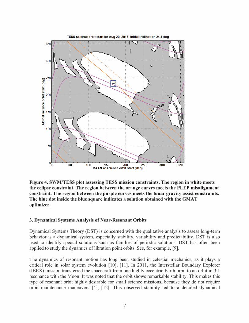
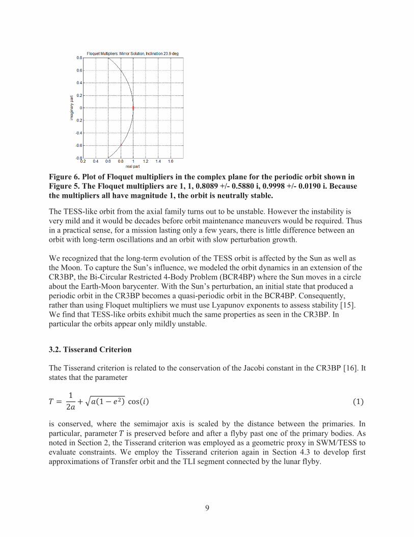
3.1. Stability Analysis In the CR3BP, the origin lies at the center of mass of the Earth and Moon; the x axis lies along the Earth-Moon direction; the z axis lies along the Moon orbit normal; and the y axis completed the orthonormal triad. The study in [13] showed that there are two families of 3-dimensional 2:1 resonant period orbits in the CR3BP, one with ‘mirror’ symmetry across the xz-plane, the other with ‘axial’ symmetry around the y axis. We identified an orbit in each family similar to the TESS orbit inclination. The TESS-like orbit with mirror symmetry is shown Figure 5. Its line of apsides is orthogonal to the line of nodes, a condition that would minimize eclipses. Figure 6 shows the Floquet multipliers for that orbit, which measure the rate of change of perturbations from that periodic orbit [14]. Because all of the multipliers have magnitude 1, the orbit in neutrally stable. In addition, the angles from the real axis of the two sets of complex multipliers indicate that perturbations exhibit one medium-term oscillation with a period of 10 lunar cycles (9 months), and a long-term oscillation with a period of 330 lunar cycles (24.7 years).

Figure 5. Top view (left) and skew view (right) of a period resonant orbit in the CR3BP with mirror symmetry across the xz-plane. The orbit is similar to the TESS orbit, with the same inclination to the lunar orbit plane, although the perigee and apogee radii are different from TESS.

9

Figure 6. Plot of Floquet multipliers in the complex plane for the periodic orbit shown in Figure 5. The Floquet multipliers are 1, 1, 0.8089 +/- 0.5880 i, 0.9998 +/- 0.0190 i. Because the multipliers all have magnitude 1, the orbit is neutrally stable.

The TESS-like orbit from the axial family turns out to be unstable. However the instability is very mild and it would be decades before orbit maintenance maneuvers would be required. Thus in a practical sense, for a mission lasting only a few years, there is little difference between an orbit with long-term oscillations and an orbit with slow perturbation growth. We recognized that the long-term evolution of the TESS orbit is affected by the Sun as well as the Moon. To capture the Sun’s influence, we modeled the orbit dynamics in an extension of the CR3BP, the Bi-Circular Restricted 4-Body Problem (BCR4BP) where the Sun moves in a circle about the Earth-Moon barycenter. With the Sun’s perturbation, an initial state that produced a periodic orbit in the CR3BP becomes a quasi-periodic orbit in the BCR4BP. Consequently, rather than using Floquet multipliers we must use Lyapunov exponents to assess stability [15]. We find that TESS-like orbits exhibit much the same properties as seen in the CR3BP. In particular the orbits appear only mildly unstable.

3.2. Tisserand Criterion The Tisserand criterion is related to the conservation of the Jacobi constant in the CR3BP [16]. It states that the parameter

is conserved, where the semimajor axis is scaled by the distance between the primaries. In particular, parameter is preserved before and after a flyby past one of the primary bodies. As noted in Section 2, the Tisserand criterion was employed as a geometric proxy in SWM/TESS to evaluate constraints. We employ the Tisserand criterion again in Section 4.3 to develop first approximations of Transfer orbit and the TLI segment connected by the lunar flyby.

10

3.3. The Kozai Mechanism for Highly Eccentric, Highly Inclination Orbits Because TESS uses a highly eccentric, highly inclined orbit, the Kozai (or Lidov-Kozai) model [17], [18] can be applied to understand the long-term behavior. The Kozai model is a version of the CR3BP, where short-term oscillations are averaged out. In this simplified model, the semimajor axis is constant, indicating that there are no long-term variations in the full force model. The Kozai parameter

cos(i) (2) is a constant of motion, where is the orbit eccentricity and is the inclination relative to the orbit plane of the primary bodies, in this case the Earth-Moon orbit plane. Moreover the eccentricity and inclination oscillate in unison. In terms more applicable to our trajectory design, the perigee radius and inclination oscillate in unison while preserving . The period of Kozai oscillation has order of magnitude

Here days is the period of the TESS spacecraft orbit, is the ratio of Earth

mass to Moon mass, and is the ratio of spacecraft orbit semimajor axis to to Moon orbit semimajor axis. (See [19], [5]) Consequently, the Kozai period is on the order of

years or 167 lunar cycles. Looking at the results in Section 3.1, the Kozai mechanism appears to explain the long-period oscillation observed for 2:1 resonant orbits. Note that the Tisserand parameter is closely related to the Kozai parameter and the fact that semimajor axis is nearly constant in the Kozai model:

(4) However, we do not use Eqn. (4) directly in our analysis. Instead we apply the Kozai mechanism to the Science orbit after PAM burn, while we apply the Tisserand criterion to the Transfer orbit and TLI segment before the PAM burn. For inclination above a critical value, The Kozai model implies that AOP librates about 90 deg or 270 deg. Thus the orbit is a kind of frozen orbit, a property that can be very useful in mission design. (In [20] and [21], Ely apply these dynamics to the design of a constellation of stable eccentric, inclined lunar orbits.) The libration of periapsis is valuable for the TESS mission. The Moon’s orbit plane lies within a few degrees of the ecliptic. If we initially place the Science orbit apogee well outside the Moon’s orbit plane, with AOP near 90 deg, then the libration of the perigee will keep apogee out of the Moon’s orbit plane, making eclipses far less likely. Kozai originally developed his model to describe the motion of small bodies in the solar system, while Lidov developed his model to describe the motion of Moon orbiting satellite perturbed by

11

the Earth. It is appropriate for the TESS mission that the Kozai mechanism has applications to exoplanet orbit dynamics [22]. The classical mechanism described by Kozai [17] neglects the effects of the Sun and the eccentricity of the Moon’s orbit. Nevertheless, in the high-fidelity (ephemeris) force model, the Kozai mechanism remains a valuable guide to qualitative long-term behavior. As describes in Section 4, Gangestad et al. [6] exploited these features effectively for the TESS trajectory design. As far as we know, Gangestad et al. were the first to exploit the Kozai mechanism for the design of a highly eccentric Earth orbit. 4. High-Fidelity Trajectory Design using GMAT and STK The two-body and three-body analysis described above was been very important to understand the orbit dynamics and to define realistic mission constraints. However for precise trajectory computation we require tools that perform numerical propagation using full force models that include the ephemerides of the Sun, Earth and Moon, as well as the Earth and Moon gravity fields. For high-fidelity propagation and for trajectory design that meets the numerous mission constraints we employ GMAT. Nevertheless, for such a complex trajectory we required two-body and three-body models to initialize the design process. Section 4.1 gives an overview of GMAT, and Section 4.2 describes how we apply GMAT to TESS trajectory design. Then in Section 4.3 we outline the process used to create a good first approximation of the several trajectory segments. Finally is Section 4.4 we describe the constrained optimization scripts developed to design the TESS trajectory and we present the results of that design. To analyze and plot the trajectory parameters we employ Analytical Graphics Inc.’s Systems Tool Kit (STK) also well as GMAT. 4.1. Overview of GMAT software

GMAT is an open-source trajectory design and optimization tool developed by NASA and private industry. It is designed to model and optimize spacecraft trajectories in flight regimes ranging from low Earth orbit to lunar, interplanetary, and other deep space missions, using built-in initial value solvers (propagators), boundary value solvers, and optimizers.

GMAT is designed with both a graphical user interface and a custom script language that exposes high-level concepts such as propagators and force models. All of the system elements can be expressed through either interface, and users can convert between the two, depending which is more advantageous to the problem at hand. A particular strength for TESS is the flexibility of the script language to allow manipulation of parameters in any coordinate system and express calculations in high-level astronautical terminology. It also contains a native interface to The Mathworks’ MATLAB® environment, allowing us to call native and custom MATLAB functions as if they were a part of the GMAT language.

GMAT’s native support for optimization is particularly attractive for this analysis because it allows the analyst to express arbitrary controls and constraints in-line with the mission execution sequence, such as before a particular maneuver is executed, or at a particular point in the optimization. This flexibility allows us to express the complex multiple-shooting optimization problems required to model the TESS trajectory.

12

4.2. Applications to scripting for TESS

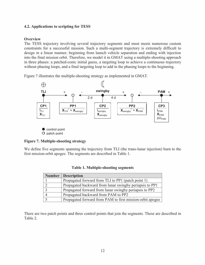
Overview The TESS trajectory involving several trajectory segments and must meets numerous custom constraints for a successful mission. Such a multi-segment trajectory is extremely difficult to design in a linear manner, beginning from launch vehicle separation and ending with injection into the final mission orbit. Therefore, we model it in GMAT using a multiple-shooting approach in three phases: a patched-conic initial guess, a targeting loop to achieve a continuous trajectory without phasing loops, and a final targeting loop to add in the phasing loops to the beginning. Figure 7 illustrates the multiple-shooting strategy as implemented in GMAT.

Figure 7. Multiple-shooting strategy

We define five segments spanning the trajectory from TLI (the trans-lunar injection) burn to the first mission-orbit apogee. The segments are described in Table 1.

Table 1. Multiple-shooting segments

Number Description 1 Propagated forward from TLI to PP1 (patch point 1) 2 Propagated backward from lunar swingby periapsis to PP1 3 Propagated forward from lunar swingby periapsis to PP2 4 Propagated backward from PAM to PP2 5 Propagated forward from PAM to first mission-orbit apogee

There are two patch points and three control points that join the segments. These are described in Table 2.

TLI PAM swingby + - + - +

CP1 tTLI XTLI

PP1 XTOI

+ = Xswingby-

CP2 tswingby Xswingby

PP2 Xswingby

+ = XPAM-

CP3 tPAM XPAM ΔVPAM

2 d 4 d

control point patch point

13

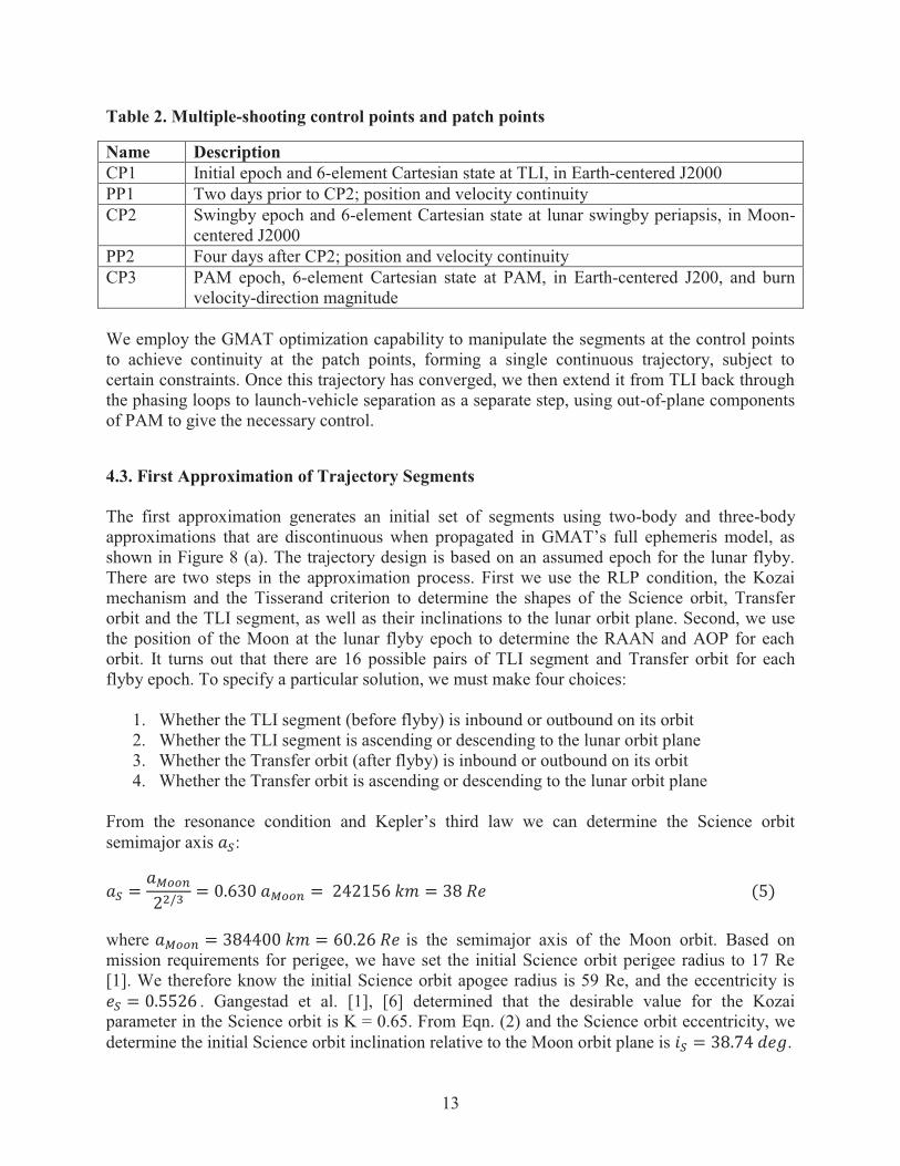
Table 2. Multiple-shooting control points and patch points

Name Description CP1 Initial epoch and 6-element Cartesian state at TLI, in Earth-centered J2000 PP1 Two days prior to CP2; position and velocity continuity CP2 Swingby epoch and 6-element Cartesian state at lunar swingby periapsis, in Moon-

centered J2000 PP2 Four days after CP2; position and velocity continuity CP3 PAM epoch, 6-element Cartesian state at PAM, in Earth-centered J200, and burn

velocity-direction magnitude We employ the GMAT optimization capability to manipulate the segments at the control points to achieve continuity at the patch points, forming a single continuous trajectory, subject to certain constraints. Once this trajectory has converged, we then extend it from TLI back through the phasing loops to launch-vehicle separation as a separate step, using out-of-plane components of PAM to give the necessary control.

4.3. First Approximation of Trajectory Segments The first approximation generates an initial set of segments using two-body and three-body approximations that are discontinuous when propagated in GMAT’s full ephemeris model, as shown in Figure 8 (a). The trajectory design is based on an assumed epoch for the lunar flyby. There are two steps in the approximation process. First we use the RLP condition, the Kozai mechanism and the Tisserand criterion to determine the shapes of the Science orbit, Transfer orbit and the TLI segment, as well as their inclinations to the lunar orbit plane. Second, we use the position of the Moon at the lunar flyby epoch to determine the RAAN and AOP for each orbit. It turns out that there are 16 possible pairs of TLI segment and Transfer orbit for each flyby epoch. To specify a particular solution, we must make four choices:

1. Whether the TLI segment (before flyby) is inbound or outbound on its orbit 2. Whether the TLI segment is ascending or descending to the lunar orbit plane 3. Whether the Transfer orbit (after flyby) is inbound or outbound on its orbit 4. Whether the Transfer orbit is ascending or descending to the lunar orbit plane

From the resonance condition and Kepler’s third law we can determine the Science orbit semimajor axis :

where is the semimajor axis of the Moon orbit. Based on mission requirements for perigee, we have set the initial Science orbit perigee radius to 17 Re [1]. We therefore know the initial Science orbit apogee radius is 59 Re, and the eccentricity is

. Gangestad et al. [1], [6] determined that the desirable value for the Kozai parameter in the Science orbit is K = 0.65. From Eqn. (2) and the Science orbit eccentricity, we determine the initial Science orbit inclination relative to the Moon orbit plane is .

14

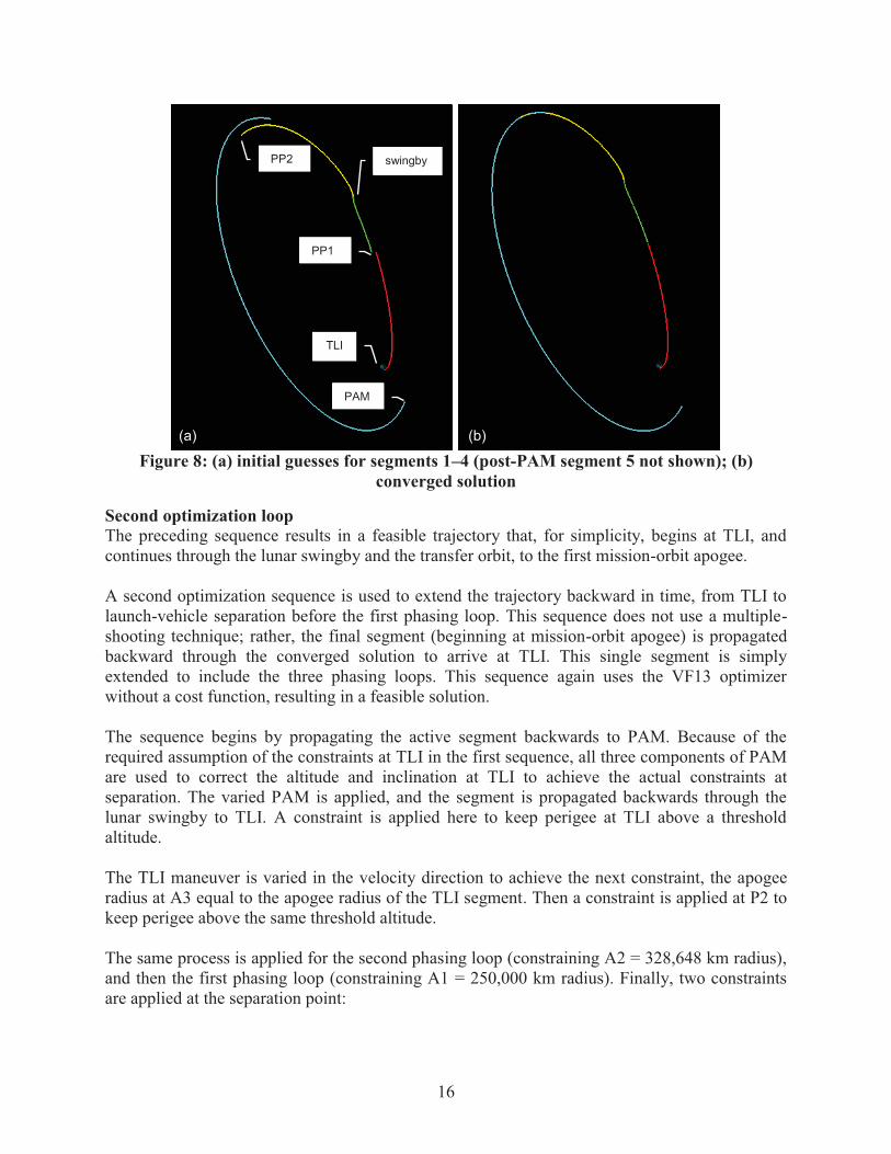
We have pointed out that the LRP condition is essential for operational stability of the Science orbit. Gangestad et al. developed an analytic approximation for the Time of Flight from flyby to PLEP to achieve the LRP condition, and found that the desired value for the Transfer orbit apogee radius is about 81 Re [6]. Because the Transfer orbit and Science orbit share the perigee radius of 17 Re, the Transfer orbit has a semimajor axis of about 49 Re. Because the Transfer orbit and Science orbit also have the same orbit inclination, from Eqn. (1) we find the Tisserand value for the Transfer orbit after the lunar flyby is about 1.147. It follows that the TLI segment before that lunar flyby also has the same Tisserand value. For the TLI segment we require that the perigee altitude be 200 km, and that the inclination to the equator is 28.5 deg. We use the position and velocity of the Moon at flyby, together with the choice of whether the orbit is ascending or descending, to determine the inclination of the TLI segment to the lunar orbit plane. The inclination to the lunar orbit plane is typically about 5 to 10 deg. The inclination and perigee radius of the TLI segment, together with the Tisserand value, determine that the apogee radius of the TLI segment. The apogee radius is typically about 61.5 Re, roughly 800 km above the Moon orbit radius. We next use the position of the Moon at flyby to compute the RAAN and AOP for the TLI segment and Transfer orbit. To determine the RAAN we use the fact that the flyby direction must be along the line of nodes for the TESS orbit, relative to the lunar orbit plane. The RAAN value for each orbit depends on whether the orbit is ascending or descending. We next determine the true anomaly at flyby, based on whether the orbit is inbound or outbound at flyby. Because the flyby is at the line of nodes, the argument of latitude is either 0 deg for an ascending solution or 180 deg for a descending solution. We can therefore use the true anomaly and the argument of latitude to determine the AOP each orbit. Because the Science orbit and the Transfer orbit are in the same plane, the RAAN and AOP for the Transfer orbit tell us the RAAN and AOP for the Science orbit. Thus far we have determined all of the orbit elements for the TLI segment, the Transfer orbit and the Science orbit. To complete the first approximation we must approximate the hyperbolic lunar flyby segment around the Moon. For this we use the velocity vectors of the pre- and post-flyby segments to determine the energy, eccentricity and orbit plane of the hyperbola using standard methods [23]. At this point in the analysis we have approximations for the four segments from TLI through lunar flyby to the Mission orbit. Figure 8 (a) shows a plot of the first approximations of the discontinuous segments for one case. The constrained optimization for blending these segments is described below. The second script combines the phasing loops with the mission trajectory already computed. The phasing loops are specified by the apogee radius values; the perigee radius of each phasing loop is nearly the same as at launch vehicle separation. The apogee and perigee radius values allow us to approximate the delta-V values for the perigee maneuvers. This algorithm generates an initial set of segments that are discontinuous when propagated in GMAT’s full ephemeris model, as shown in Figure 8 (a).

15

4.4. GMAT Constrained Optimization Scripts

First optimization loop The primary optimization sequence uses the initial guesses at the three control points (CP1–CP3) to achieve continuity at the two patch points (PP1 and PP2) while meeting certain mission-level constraints. The Harwell Subroutine Library Sequential Quadratic Programming (SQP) VF13 optimizer is used with no cost function, giving a feasible solution. The sequence begins by varying the epochs of the three control points, and then derives the epochs of the two patch points from the epoch of CP2. The Cartesian states of all control points are varied, along with the velocity-direction component of PAM. Then, the two mirrored segments (segment #3 mirrored from segment #2, and segment #5 mirrored from segment #4) are initialized by duplicating the states. Six constraints are enforced just after initialization, when the segments are at their initial conditions:

� Inclination to equator at TLI = 28.5° � Altitude of perigee at TLI = 200 km � Radius of perigee at PAM = 17 Re � TLI occurs at perigee � PAM occurs at perigee � Mission orbit misalignment at PAM ≤ 30°

After propagating segments #1–4 to the two patch points, continuity constraints are applied for the full six-element Cartesian states. Finally, segment #5 is propagated to mission-orbit apogee, and a final constraint is applied:

� Energy = energy at semi-major axis required for 2:1 lunar resonance The initial guess and final converged solution are shown in Figure 8.

16

Figure 8: (a) initial guesses for segments 1–4 (post-PAM segment 5 not shown); (b)

converged solution

Second optimization loop The preceding sequence results in a feasible trajectory that, for simplicity, begins at TLI, and continues through the lunar swingby and the transfer orbit, to the first mission-orbit apogee. A second optimization sequence is used to extend the trajectory backward in time, from TLI to launch-vehicle separation before the first phasing loop. This sequence does not use a multiple-shooting technique; rather, the final segment (beginning at mission-orbit apogee) is propagated backward through the converged solution to arrive at TLI. This single segment is simply extended to include the three phasing loops. This sequence again uses the VF13 optimizer without a cost function, resulting in a feasible solution. The sequence begins by propagating the active segment backwards to PAM. Because of the required assumption of the constraints at TLI in the first sequence, all three components of PAM are used to correct the altitude and inclination at TLI to achieve the actual constraints at separation. The varied PAM is applied, and the segment is propagated backwards through the lunar swingby to TLI. A constraint is applied here to keep perigee at TLI above a threshold altitude. The TLI maneuver is varied in the velocity direction to achieve the next constraint, the apogee radius at A3 equal to the apogee radius of the TLI segment. Then a constraint is applied at P2 to keep perigee above the same threshold altitude. The same process is applied for the second phasing loop (constraining A2 = 328,648 km radius), and then the first phasing loop (constraining A1 = 250,000 km radius). Finally, two constraints are applied at the separation point:

TLI

swingby

PAM

PP1

PP2

(a) (b)

17

� Altitude at launch-vehicle separation = 200 km � Inclination at launch-vehicle separation = 28.5°

Once converged, this two-part strategy results in a full, continuous, feasible trajectory for the entire mission, from launch-vehicle separation through the first mission-orbit apogee. The mission orbit can then be propagated forward for the entire mission lifetime with no additional controls.

Results Results to date are all derived from point-solution initial guesses found numerically, rather than from the in-development patched-conic method. In total, there are 9 solutions that converge using the multiple-shooting method. These are summarized in Table 3.

Table 3. GMAT delta-V simulation results (m/s)

Separation Epoch

24 Mar 2017

18 Apr 2017

15 May 2017

16 May 2017

14 Jun 2017

12 Jul 2017

12 Jan 2018

18 Jan 2018

19 Jan 2018

A1 29.5 2.9 2.3 5.0 18.3 21.0 7.9 58.5 26.9 P1 37.8 33.4 33.4 34.2 37.5 38.3 28.0 41.0 38.2 P2 20.1 21.0 21.3 20.5 19.7 19.7 27.7 21.4 19.6 TLI 4.2 14.8 15.6 12.4 2.2 -1.0 25.7 4.2 1.6 PAM x -85.6 -85.8 -86.6 -83.4 -76.9 -83.4 -94.3 -94.3 -90.9 PAM y -1.5 -1.8 3.6 7.8 -2.6 -3.3 -2.6 -21.7 -5.5 PAM z 1.0 1.0 -0.3 -1.3 0.9 0.8 -0.6 4.8 1.1 PAM dv 85.6 85.8 86.7 83.8 76.9 83.5 94.3 96.9 91.1 Total (m/s) 177.2 158.0 159.2 155.9 154.6 163.5 183.6 222.1 177.4

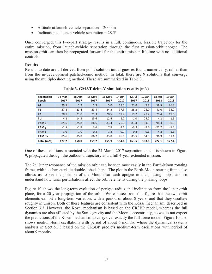
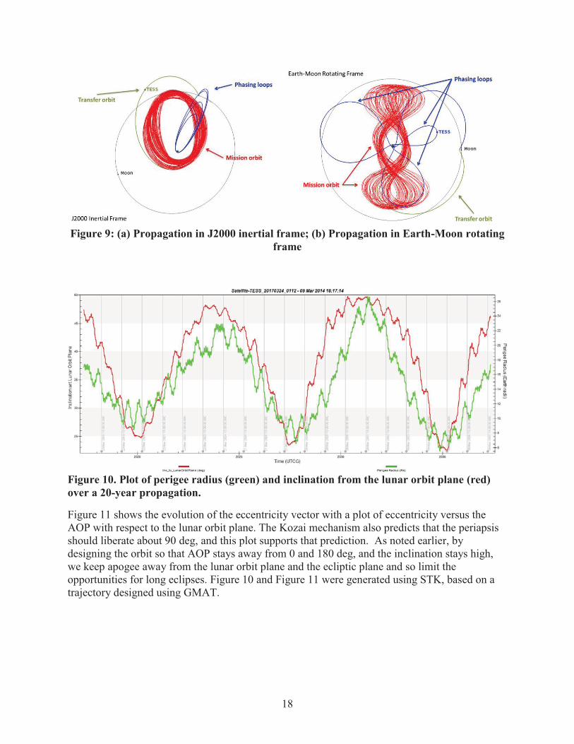
One of these solutions, associated with the 24 March 2017 separation epoch, is shown in Figure 9, propagated through the outbound trajectory and a full 4-year extended mission. The 2:1 lunar resonance of the mission orbit can be seen most easily in the Earth-Moon rotating frame, with its characteristic double-lobed shape. The plot in the Earth-Moon rotating frame also allows us to see the position of the Moon near each apogee in the phasing loops, and so understand how lunar perturbations affect the orbit elements during the phasing loops. Figure 10 shows the long-term evolution of perigee radius and inclination from the lunar orbit plane, for a 20-year propagation of the orbit. We can see from this figure that the two orbit elements exhibit a long-term variation, with a period of about 8 years, and that they oscillate roughly in unison. Both of these features are consistent with the Kozai mechanism, described in Section 3.3. However, the Kozai mechanism is based on the CR3BP model, whereas the full dynamics are also affected by the Sun’s gravity and the Moon’s eccentricity, so we do not expect the predictions of the Kozai mechanism to carry over exactly the full-force model. Figure 10 also shows medium-term oscillations with period of about 6 months, where the dynamical systems analysis in Section 3 based on the CR3BP predicts medium-term oscillations with period of about 9 months.

18

Figure 9: (a) Propagation in J2000 inertial frame; (b) Propagation in Earth-Moon rotating

frame

Figure 10. Plot of perigee radius (green) and inclination from the lunar orbit plane (red) over a 20-year propagation.

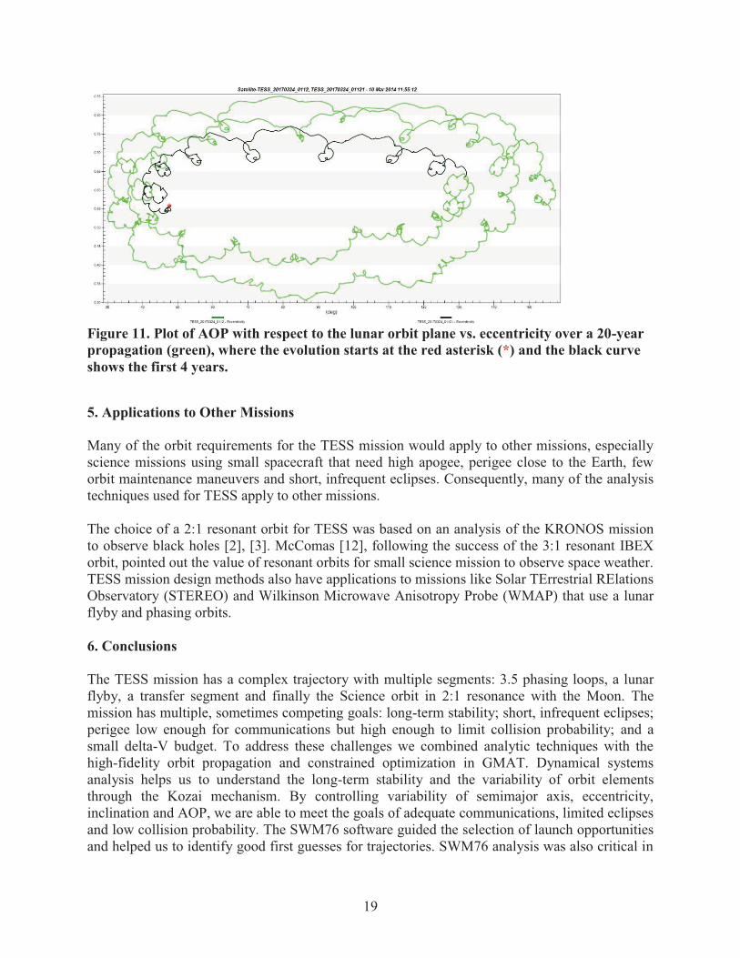
Figure 11 shows the evolution of the eccentricity vector with a plot of eccentricity versus the AOP with respect to the lunar orbit plane. The Kozai mechanism also predicts that the periapsis should liberate about 90 deg, and this plot supports that prediction. As noted earlier, by designing the orbit so that AOP stays away from 0 and 180 deg, and the inclination stays high, we keep apogee away from the lunar orbit plane and the ecliptic plane and so limit the opportunities for long eclipses. Figure 10 and Figure 11 were generated using STK, based on a trajectory designed using GMAT.

19

Figure 11. Plot of AOP with respect to the lunar orbit plane vs. eccentricity over a 20-year propagation (green), where the evolution starts at the red asterisk (*) and the black curve shows the first 4 years.

5. Applications to Other Missions Many of the orbit requirements for the TESS mission would apply to other missions, especially science missions using small spacecraft that need high apogee, perigee close to the Earth, few orbit maintenance maneuvers and short, infrequent eclipses. Consequently, many of the analysis techniques used for TESS apply to other missions. The choice of a 2:1 resonant orbit for TESS was based on an analysis of the KRONOS mission to observe black holes [2], [3]. McComas [12], following the success of the 3:1 resonant IBEX orbit, pointed out the value of resonant orbits for small science mission to observe space weather. TESS mission design methods also have applications to missions like Solar TErrestrial RElations Observatory (STEREO) and Wilkinson Microwave Anisotropy Probe (WMAP) that use a lunar flyby and phasing orbits. 6. Conclusions The TESS mission has a complex trajectory with multiple segments: 3.5 phasing loops, a lunar flyby, a transfer segment and finally the Science orbit in 2:1 resonance with the Moon. The mission has multiple, sometimes competing goals: long-term stability; short, infrequent eclipses; perigee low enough for communications but high enough to limit collision probability; and a small delta-V budget. To address these challenges we combined analytic techniques with the high-fidelity orbit propagation and constrained optimization in GMAT. Dynamical systems analysis helps us to understand the long-term stability and the variability of orbit elements through the Kozai mechanism. By controlling variability of semimajor axis, eccentricity, inclination and AOP, we are able to meet the goals of adequate communications, limited eclipses and low collision probability. The SWM76 software guided the selection of launch opportunities and helped us to identify good first guesses for trajectories. SWM76 analysis was also critical in

*

20

trade studies to determine the battery size needed to handle eclipses and still have adequate launch opportunities. We employed the excellent analysis by Gangestad et al. [Gangestad] to create a good first approximation for an arbitrary lunar flyby epoch. We then exploit the capabilities in GMAT to perform constrained optimization with multiple shooting to generate a continuous trajectory with minimum delta-V that meets mission requirements. The analytical and numerical tools that we have employed successfully for the TESS mission have broader applications to other science missions with small spacecraft. Acknowledgements The trajectory analysis performed at NASA Goddard Space Flight Center was funded by the TESS project. The Dynamical Systems analysis of the IBEX and TESS orbits was performed at Applied Defense Solutions in 2010 to 2012. The original trajectory work using GMAT was performed by Sonia Hernandez and Steven Hughes. We thank Steven Hughes for his peer review that helped us to clarify some key points in this paper.

Bibliography [1] G. Ricker, "Transiting Exoplanet Survey Satellite (TESS) Concept Study Report (CSR)," MIT, 2012. [2] M. Mathews, M. Hametz and J. S. D. Cooley, "High Earth Design for Lunar Assisted Small Explorer Class

Missions," in Flight Mechanics/Estimation Theory Symposium, Greenbelt MD, 1994. [3] D. McGiffin, M. Mathews and S. Cooley, "High Earth Orbit Desing for Lunar Asisted Medium Class Explorer

Missions," in Flight MEchanics Symposium, Greenbelt MD, 2001. [4] J. Carrico, D. Dichmann and L. Policastri, "Lunar-Resonant Trajectory Design for the Interstellar Boundary

Explorer (IBEX) Extended Mission," in AAS/AIAA Astrodynamical Specialist Conference, Girdwood AK, 2011.

[5] D. Dichmann, R. Lebois and J. Carrico, "Dynamics of Orbits near 2:1 Resonance in the Earth-Moon System," Journal of Astronautical Sciences, 2013 (accepted).

[6] J. Gangestad, G. Hennings, G. Ricker and R. Persinger, "Design of a Resonant Orbit," in AAS/AIAA Astrodynamics Specialist Conference, Savannah GA, 2013.

[7] T. Williams, "Launch Window Analysis For The Magnetospheric Multiscale Mission," in AAS/AIAA Space Flight Mechanics Meeting, Charleston, SC, 2012.

[8] R. Bate, D. Mueller and J. White, Fundamentals of Astrodynamics, Dover, 1971. [9] B. Barden, K. Howell and M. Lo, "Application of Dynamical Systems Theory to Trajectory Design for a

Libration Point Mission," J. Astronautical Sciences, vol. 45, no. 2, pp. 161-178, Apr-Jun 1997. [10] C. Murray and S. Dermott, Solar System Dynamics, Cambridge: Cambridge University Press, 1999. [11] A. Morbidelli, Modern Celestial Mechanics: Aspects of Solar System Dynamics, Taylor & Francis, 2002. [12] D. McComas, J. Carrico, B. Hautamaki, M. Intelisano, R. Lebois, M. Loucks and L. Policatri, "A new class of

long–term stable lunar resonance orbits: Space weather applications and the Interstellar Boundary Explorer," Space Weather, vol. 9, 2011.

[13] D. Dichmann, "Dynamical Systems Analysis of TESS Mission Orbit," Applied Defense Solutions, NASA Goddard Space Flight Center, Greenbelt MD, 2012.

[14] K. Meyer and G. Hall, Introduction to Hamiltonian Dynamics and the N-Body Problem, New York: Springer, 1992.

[15] T. Parker and L. Chua, Practical Numerical Algorithms for Chaotic Systems, New York: Springer, 1989. [16] J. Danby, Fundamentals of Celestial Mechanics, Richmond VA: Willmann-Bell, 1998.

21

[17] Y. Kozai, "Secular perturbations of asteroids with high inclination and high eccentricity," Astron. J. , vol. 67, p. 591, 1962.

[18] M. Lidov, "The Evolution of Orbits of Artificial Satellites of Planets under the Action of Gravitational Perturbations of External Bodies," Planetary and Space Science, vol. 9, pp. 719-759, 1962.

[19] T. Mazeh and J. Shaman, "The Orbital Evolution of Close Triple Systems: The Binary Eccentricity," Astron. Astrophys., vol. 77, pp. 145-151, 1979.

[20] T. Ely, "Stable Constellations of Frozen Ellptical Inclined Lunar Orbits," J. Astronautical Sciences, vol. 53, no. 3, pp. 301-316, 2005.

[21] T. Ely and E. Lieb, "Constellations of Elliptical Inclined Lunar Orbits Providing Polar and Global Coverage," in AAS/AIAA Astrodynamics Specialist Conference, Lake Tahoe, CA, 2005.

[22] A. Correia and J. Laskar, "Tidal Evolution of Exoplanets," in Exoplanets, Tucson, AZ: University of Arizone Press, 2010, pp. 239-266.

[23] M. Kaplan, Modern Spacecraft Dynamics & Control, Wiley, 1976.