trajectory planning and feedforward design for ... · 12 trajectory planning and feedforward design...
TRANSCRIPT
12
Trajectory planning and feedforward designfor electromechanical motion systems
version 2
Report nr. DCT 2003-18
Paul LambrechtsEmail: [email protected]
April 1, 2003
Abstract
This report considers trajectory planning with constrained dynamics and design of an appro-priate feedforward controller for single axis motion control. A motivation is given for usingmodel-based fourth order feedforward with fourth order trajectories. An algorithm is givenfor calculating higher order trajectories with bounds on all considered derivatives for point topoint moves. It is shown that these trajectories are time-optimal in the most relevant cases.All required equations for third and fourth order trajectory planning are explicitly derived.Implementation, discretization and quantization effects are considered. Simulation resultsshow the superior effectiveness of fourth order feedforward in comparison with rigid-bodyfeedforward.This report differs from DCT 2003-08 in that it contains an improved algorithm for fourthorder trajectory planning (total absence of iteration loops).
1
m 1 m 2
Contents
1 Introduction 3
2 Rigid-body feedforward 6
3 Higher order feedforward 8
4 Higher order trajectory planning 10
5 Third order trajectory planning 13
6 Fourth order trajectory planning 176.1 Main algorithm 176.2 Solution of equation 49 23
7 Implementation aspects 257.1 Switching times 257.2 Synchronization of profiles 267.3 Implementation of first order filter 287.4 Calculation of reference trajectory 29
8 Simulation results 30
9 Conclusions 34
A List of symbols 36
B The Matlab function MAKE4.m 37
2
m 1 m 2
1 Introduction
Feedforward control is a well known technique for high performance motion control problems asfound in industry. It is, for instance, widely applied in robots, pick-and-place units and position-ing systems. These systems are often embedded in a factory automation scheme, which providesdesired motion tasks to the considered system. Such a motion task can be to perform a motionfrom a position A to a position B, starting at a time t.
Usually this task is transferred to computer hardware dedicated to the control of the system,leaving the details of planning and execution of the motion to this dedicated motion controlcomputer. The tasks of this dedicated motion controller will then consist of:
• trajectory planning: the determination of an allowable trajectory for all degrees of freedom,separately or as a multidimensional trajectory, and the calculation of an allowable trajectoryfor each actuation device;
• feedforward control: the representation of the desired trajectory in appropriate form andthe calculation of a feedforward control signal for each actuation device, with the intentionto obtain the desired trajectory;
• system compensation: to reduce or remove unwanted behavior like known or measureddisturbances and non-linearities;
• feedback control: the processing of available measurements and calculation of a feedbackcontrol signal for each actuation device to compensate for unknown disturbances and un-modelled behavior,
• internal checks, diagnostics, safety issues, communication, etc.
To simplify the tasks of the motion controller, the trajectory planning and feedforward control areusually done for each actuating device separately, relying on system compensation and feedbackcontrol to deal with interactions and non-linearities. In that case, each actuating device is con-sidered to be acting on a simple object, usually a single mass, moving along a single degree offreedom. The feedforward control problem is then to generate the force required to perform theacceleration of the mass in accordance with the desired trajectory.
Conversely, the desired trajectory should be such that the required force is allowable (in thesense of mechanical load on the system) and can be generated by the actuating device. For obvi-ous reasons this approach is often referred to as ‘mass feedforward’ or ‘rigid-body feedforward’.It allows a simple and practical implementation of both trajectory planning and feedforward con-trol, as the required calculations are straightforward.
The disadvantage of this approach is its dependence on system compensation and feedback con-trol to deal with unmodelled behavior as mentioned before. The resulting problem formulationcan be split in two.
1. During execution of the trajectory the position errors are large, such that feedback con-trol actions are considerable. Actual velocity and acceleration (hence: actuator force) maytherefore be much larger than planned. This may lead to undesired and even dangerousdeviations from the planned trajectory and damage to actuator and system.
3
m 1 m 2
2. When arriving at the desired endpoint, the positioning error is large and the dynamicalstate of the controlled system is not settled. Although the trajectory has finished, it isoften necessary to wait for a considerable time before the position error is settled withinsome given accuracy bounds before subsequent actions or motions are allowed. A practicalconsequence is the need for of a complex test to determine whether settling has sufficientlyoccurred. Furthermore, it is a source of time uncertainty that may be undesirable on thefactory automation level.
To improve on this, many academic and practical approaches are possible. These can roughly becategorized in three.
1. Trajectory smoothing or shaping: This can be done by simply reducing the accelerationand velocity bounds used for trajectory planning, but also by smoothing or shaping thetrajectory and/or application of force (higher order trajectories, S-curves, input shaping,filtering). The result of this can be very good, especially if the dynamical behavior of themotion system is explicitly taken into account. However, it may also lead to a considerableincrease in execution time of the trajectory, often without a clear mechanism for finding atime optimal solution. Various examples of this approach can be found in [4, 7, 8, 9, 13, 6].
2. Feedforward control based on plant inversion: This attempts to take the effect of unmod-elled behavior into account by either using a more detailed model of the motion systemor by learning its behavior based on measurements. An important practical disadvantageis that they do not provide an approach for designing an appropriate trajectory. Variousexamples of this approach can be found in [3, 5, 10, 11, 12, 15, 16, 17].
3. Feedback control optimization (possibly aided by system compensation improvement): Byimproving the feedback controller, the positioning errors can be kept smaller during and atthe end of the trajectory. Furthermore, settling will occur in a shorter time. Also in this casethe design of an appropriate trajectory is not considered. Obviously, any feedback controldesign method can be used for this. Some references given above also include a discussionon the effect of feedback control on trajectory following; e.g. see [11, 12, 17].
This report will provide a method for higher order trajectory planning that can be used withall of the approaches given above. It is attempted to give a better understanding of the effectof smoothing, especially when considering a more optimal balancing between time optimality,physical bounds (actuator device and motion system limits) and accuracy.
‘Fourth order feedforward’ will be presented as a clear and well implementable extension ofrigid-body feedforward, with also a clear strategy for obtaining the aforementioned optimal bal-ance. The implementation of a fourth order trajectory planner will be set up as a natural extensionof second and third order planners to show the potential for practical application. Furthermore,the calculation of the optimal feedforward control signal will be shown.
Next the effect of discrete time implementation will be considered: this includes the planningof a fourth order trajectory in discrete time and the optimal compensation of time delays in thefeedforward control signal. Finally, some simulation results are given to further motivate the useof fourth order feedforward.
The next chapter will review rigid-body feedforward, mostly with the purpose of introducing somenotation. Next, chapter 3 will consider the extension of mass feedforward to fourth order feedfor-ward, based on an extended model of the motion system. A general algorithm for higher order
4

m 1 m 2
trajectory planning will be considered in chapter 4, after which the relevant equations are derivedfor third order trajectory planning in chapter 5 and for fourth order trajectory planning in chap-ter 6. Next, implementation aspects are considered in chapter 7, followed by some simulationresults in chapter 8, and conclusions in chapter 9.
5
m 1 m 2
2 Rigid-body feedforward
The specifics of planning a trajectory and calculating a feedforward signal based on rigid-bodyfeedforward are fairly simple and can be found in many commercially available electromechani-cal motion control systems. In this chapter a short review is given as an introduction to a stan-dardized approach to third and fourth order feedforward calculations.
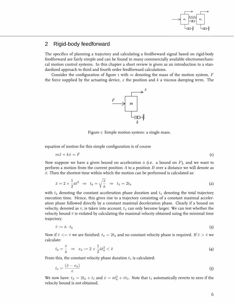
Consider the configuration of figure 1 with m denoting the mass of the motion system, Fthe force supplied by the actuating device, x the position and k a viscous damping term. The
F m
x
kFigure 1: Simple motion system: a single mass.
equation of motion for this simple configuration is of course
mx + kx = F (1)
Now suppose we have a given bound on acceleration a (i.e. a bound on F ), and we want toperform a motion from the current position A to a position B over a distance we will denote asx. Then the shortest time within which the motion can be performed is calculated as:
x = 2× 12at2 ⇒ ta =
√x
a⇒ tx = 2ta (2)
with ta denoting the constant acceleration phase duration and tx denoting the total trajectoryexecution time. Hence, this gives rise to a trajectory consisting of a constant maximal acceler-ation phase followed directly by a constant maximal deceleration phase. Clearly if a bound onvelocity, denoted as v, is taken into account, tx can only become larger. We can test whether thevelocity bound v is violated by calculating the maximal velocity obtained using the minimal timetrajectory:
v := a · ta (3)
Now if v <= v we are finished: tx = 2ta and no constant velocity phase is required. If v > v wecalculate:
ta =v
a⇒ xa := 2× 1
2at2a < x (4)
From this, the constant velocity phase duration tv is calculated:
tv =(x− xa)
v(5)
We now have: tx = 2ta + tv and x = at2a + vtv. Note that tv automatically reverts to zero if thevelocity bound is not obtained.
6
m 1 m 2
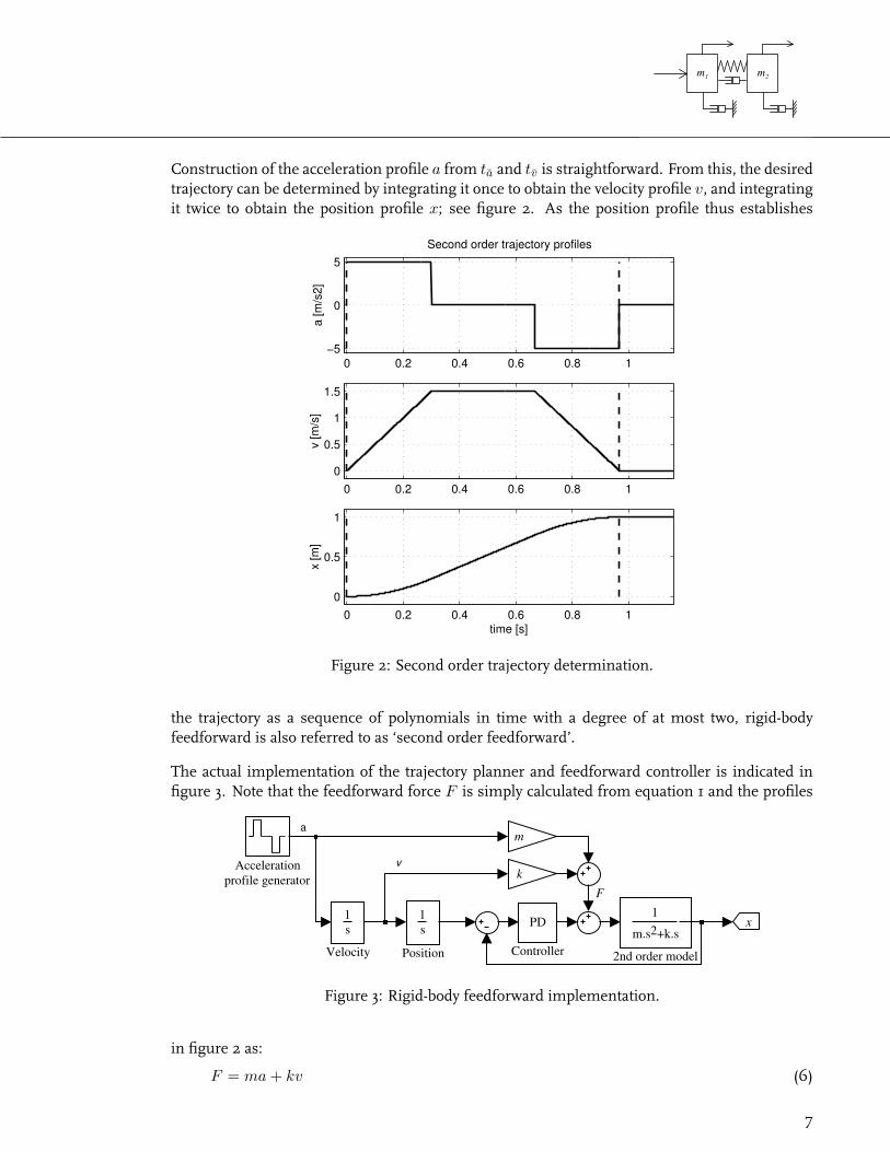
Construction of the acceleration profile a from ta and tv is straightforward. From this, the desiredtrajectory can be determined by integrating it once to obtain the velocity profile v, and integratingit twice to obtain the position profile x; see figure 2. As the position profile thus establishes
0 0.2 0.4 0.6 0.8 1−5
0
5Second order trajectory profiles
a [m
/s2]
0 0.2 0.4 0.6 0.8 10
0.5
1
1.5
v [m
/s]
0 0.2 0.4 0.6 0.8 10
0.5
1
time [s]
x [m
]
Figure 2: Second order trajectory determination.
the trajectory as a sequence of polynomials in time with a degree of at most two, rigid-bodyfeedforward is also referred to as ‘second order feedforward’.
The actual implementation of the trajectory planner and feedforward controller is indicated infigure 3. Note that the feedforward force F is simply calculated from equation 1 and the profiles
F
a
vk
m
1s
Velocity
1s
Position
xPD
Controller
Accelerationprofile generator
1
m.s +k.s2
2nd order model
Figure 3: Rigid-body feedforward implementation.
in figure 2 as:
F = ma + kv (6)
7
m 1 m 2
3 Higher order feedforward
The previous chapter shows that mass feedforward is based on a simple single mass model ofthe motion system. This implies that the performance of rigid-body feedforward is determinedby how much the actual motion system deviates from this single mass model.
On the other hand, the performance of the motion system as a whole is also determined bythe quality of system compensation and/or feedback control. It can be stated that the success offeedback control is such that in many cases the mass feedforward approach is considered suffi-cient, given that an appropriate feedback controller is required anyway for disturbance reductionand stabilization.
However, when considering further improvement of motion control system performance, theuse of higher order feedforward is often a very effective approach in comparison with improvedfeedback control. The first effect is that higher order trajectories inherently have a lower energycontent at higher frequencies, which results in a lower high frequency content of the error sig-nal, which in turn enables the feedback controller to be more effective. The second effect is thathigher order trajectories have less chance of demanding a motion which is physically impossibleto perform by the given motion system: e.g. most power amplifiers exhibit a ‘rise time’ effect,such that it is impossible to produce a step-like change in force.
These effects are commonly referred to as ‘smoothing’ and result in a decrease of positioningerrors during execution of the trajectory and a reduced settling time. The disadvantage of higherorder trajectories, i.e. the increase in trajectory execution time, is usually more than compensatedby the reduced settling time. Because of this, many high performance motion systems are alreadyequipped with a third order trajectory planner as a direct extension of mass feedforward. In thischapter it will be determined that a fourth order trajectory planner and feedforward calculationgives a significant further improvement.
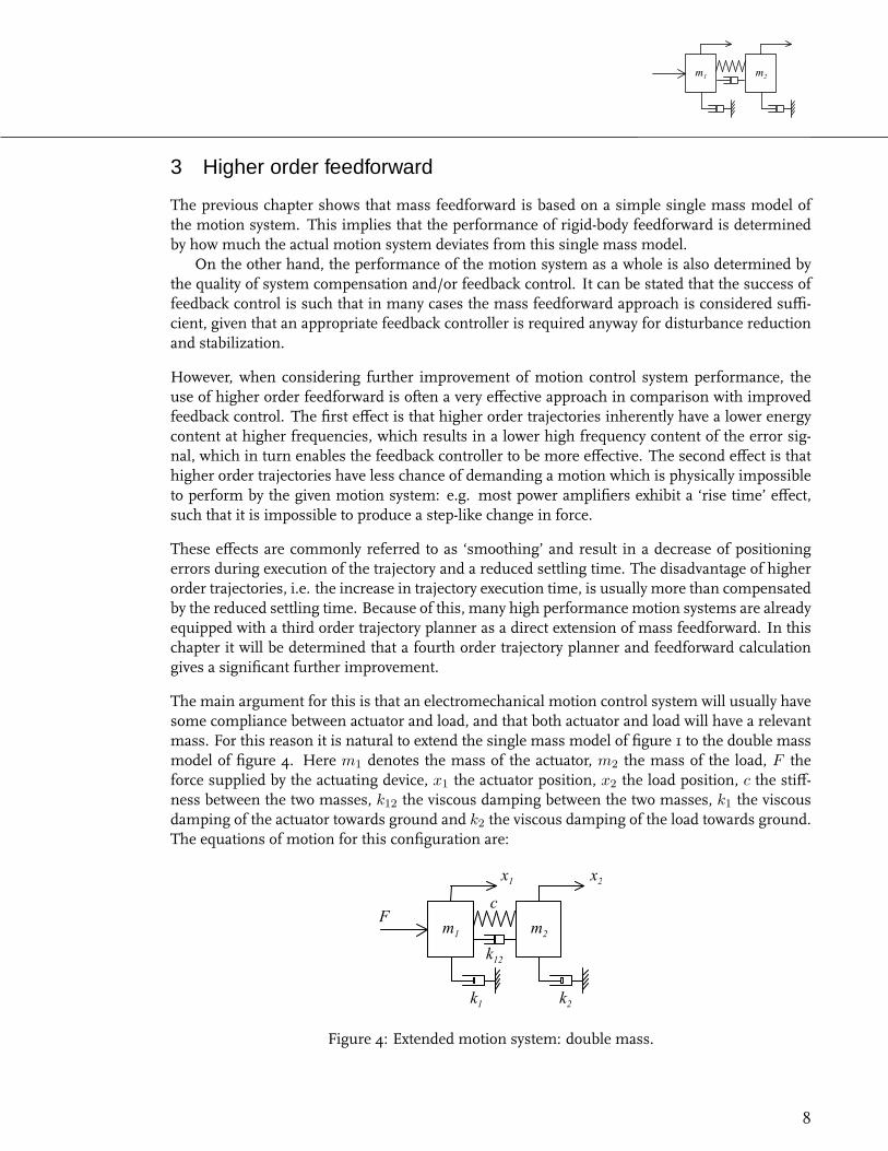
The main argument for this is that an electromechanical motion control system will usually havesome compliance between actuator and load, and that both actuator and load will have a relevantmass. For this reason it is natural to extend the single mass model of figure 1 to the double massmodel of figure 4. Here m1 denotes the mass of the actuator, m2 the mass of the load, F theforce supplied by the actuating device, x1 the actuator position, x2 the load position, c the stiff-ness between the two masses, k12 the viscous damping between the two masses, k1 the viscousdamping of the actuator towards ground and k2 the viscous damping of the load towards ground.The equations of motion for this configuration are:
F m 1
x 1
k 1
m 2
x 2
k 2
c
k 1 2
Figure 4: Extended motion system: double mass.
8
m 1 m 2
{m1x1 = −k1x1 − c(x1 − x2)− k12(x1 − x2) + Fm2x2 = −k2x2 + c(x1 − x2) + k12(x1 − x2)
(7)
Laplace transformation and substitution then results in the following expression:
F =q1s
4 + q2s3 + q3s
2 + q4s
k12s + c· x2 (8)
with: q1 = m1m2
q2 = (m1 + m2)k12 + m1k2 + m2k1
q3 = (m1 + m2)c + k1k2 + (k1 + k2)k12
q4 = (k1 + k2)c
(9)
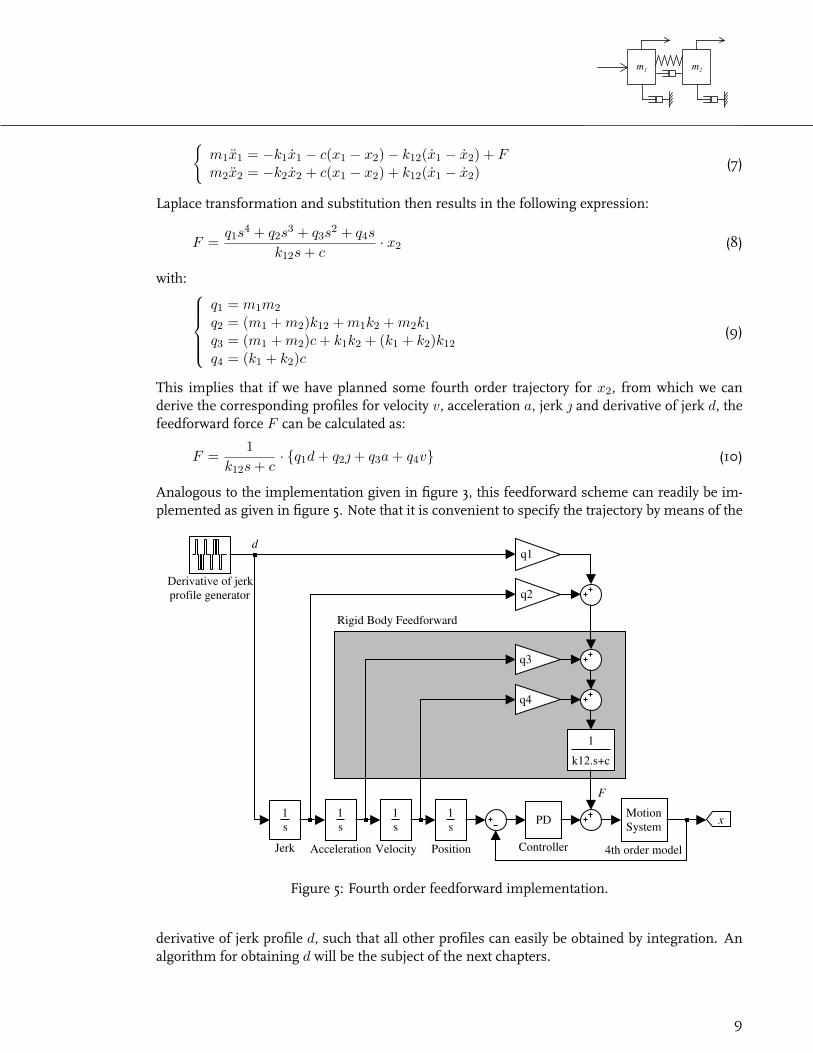
This implies that if we have planned some fourth order trajectory for x2, from which we canderive the corresponding profiles for velocity v, acceleration a, jerk and derivative of jerk d, thefeedforward force F can be calculated as:
F =1
k12s + c· {q1d + q2 + q3a + q4v} (10)
Analogous to the implementation given in figure 3, this feedforward scheme can readily be im-plemented as given in figure 5. Note that it is convenient to specify the trajectory by means of the
F
d
Rigid Body Feedforward
q1
q2
q4
q3
1
k12.s+c
1s
Velocity
1s
Position
1s
Jerk
x
Derivative of jerkprofile generator
PD
Controller
1s
Acceleration
MotionSystem
4th order model
Figure 5: Fourth order feedforward implementation.
derivative of jerk profile d, such that all other profiles can easily be obtained by integration. Analgorithm for obtaining d will be the subject of the next chapters.
9
m 1 m 2
4 Higher order trajectory planning
Planners for second and third order trajectories are fairly well known in industry and academiaand there are many approaches for obtaining a valid solution. Extension to fourth order trajectoryplanning is however not trivial. In this chapter we will review the main objectives of trajectoryplanning in general and set up an algorithm for obtaining these objectives more or less irrespec-tive of the order of the resulting trajectory.
As mentioned before, a trajectory is usually planned for a motion from the current position A tosome desired end position B under some boundary constraints. This will also be the basis for thediscussion given here, although the resulting algorithm can be adjusted for relevant alternativeobjectives like for instance speed control instead of position control, scanning motions or speedchange operations.
Several further objectives that are of importance for applicability of a trajectory planning al-gorithm are given below.
• Timing. In principle we should strive for time optimality; at least it must be clear what theconsequences are for the trajectory execution time when considering the effect of boundaryconditions.
• Actuator effort. This is usually the basis for the selection of bounds for velocity, accelerationand jerk, although they may also be related to bounds on mechanics or safety issues.
• Accuracy. For point to point moves, the planned end position of the trajectory must beequal to the desired end position (within measurement accuracy).
• Complexity. Usually trajectory planning is thought of as being done off-line. In practicehowever, the desired end position often becomes available at the moment the trajectoryshould start. Hence, the time required for planning the trajectory is lost and should beminimized.
• Reliability. The planning algorithm should always come up with a valid solution.
• Implementation. Trajectory planning is done in computer hardware, and is therefore sub-ject to discretization and digitization.
Now we argue that these objectives, except the final one, are all met by the simple algorithm givenin chapter 2:
1. calculate ta =√
xa (equation 2),
2. calculate v = a · ta (equation 3),
3. test v > v:
• if true recalculate ta = va (equation 4),
• if false: no action,
4. calculate xa = at2a (equation 4),
5. calculate tv = (x−xa)v (equation 5), and
10
m 1 m 2
6. finished: x = at2a + vtv and tx = 2ta + tv.
First consider timing; obviously timing is minimal if the bound on v is discarded as is done instep 1. If introducing this bound leads to a reduction of ta (verify that equation 4 always leadsto a reduction) the result will be that v = v is obtained in the shortest possible time, and iscontinued for as long as possible. Hence the trajectory execution time is always minimal, giventhe bounds a and v. Next, actuator effort is immediately taken into account by means of the givenbounds, accuracy is precise, complexity is low and reliability is high (no iteration loops that canhang up, algorithm only fails if a non-positive bound is specified). The implementation problemis considered later.
Given the advantages of this algorithm, it is desirable to generalize it for planning higherorder trajectories. The position displacement x and bounds on all derivatives of the trajectory upto the highest order derivative d (indicated as d) are assumed to be given. Furthermore we willrequire that all derivatives are equal to zero at the start and end positions.
1. Determine a symmetrical trajectory that has d equal to either d or −d at all times andobtains displacement x.
2. Determine td: the shortest time that d remains constant (always the first period).
3. Calculate the maximal value of velocity v obtained during this trajectory.
4. Test v > v:
• if true re-calculate td based on v (td decreases),
• if false continue.
5. Calculate the maximal value of acceleration a obtained during this trajectory.
6. Test a > a:
• if true re-calculate td based on a (td decreases),
• if false continue.
7. Continue these tests and possible recalculations until d; the last test is performed on ,defined as the highest derivative before d. The resulting td will not be changed anymore.
8. Extend the trajectory symmetrically with periods of constant whenever reaches the value or −: this must be done such that the required displacement x is obtained.
9. Determine t: the shortest time that remains constant.
10. Starting with velocity and ending with the derivative before , calculate the maximal valueand re-calculate t if the appropriate bound is violated (each re-calculation can only decreaset).
11. The resulting t will not be changed anymore.
12. Extend the trajectory symmetrically with periods of constant next lower derivative; againsuch that the required displacement x is obtained. Determine the associated time intervaland do the tests and recalculations resulting in a final value for it.
11
m 1 m 2
13. Continue until v: the constant speed phase duration tv is calculated such that the requireddisplacement x is obtained (i.e. the displacement ‘left to go’ divided by v).
14. Finished: td, t, etc. until tv completely determine the trajectory.
The properties of the resulting trajectories (in the sense of the objectives given above) appearto depend partly on the order of the trajectory planner. Obviously, the required calculations be-come more complex with increasing order. Time-optimality is still automatically obtained withthird order trajectories, but not necessarily for fourth order trajectories (this can be obtained butcosts much complexity at a small gain with respect to a good sub-optimal solution). In principle,higher than fourth order trajectories can also be planned by means of this algorithm, but this isconsidered impractical due to the large increase in complexity. It is noted here that all calculationsfor third and fourth order planning can be done analytically with fairly basic mathematical func-tions, except one calculation for fourth order planning. For this case a simple and numericallystable search algorithm can be used.
The next chapter will provide the calculations for third order trajectory planning; after thatfourth order trajectory planning will be considered.
12
m 1 m 2
5 Third order trajectory planning
Although chapter 3 shows that fourth order trajectory planning and feedforward is strongly mo-tivated by a model based approach, it may still be useful to apply third order trajectory planning.This chapter will provide the derivations and calculations necessary to ‘fill in’ the algorithm de-veloped in chapter 4 for third order trajectory planning.
We will assume that a trajectory must be planned over a distance x, that bounds are givenon velocity (v), acceleration (a) and jerk (), and that the trajectory must be time optimal withinthese bounds. The bound on jerk can for instance be related to ‘rise time’ behavior as commonlyfound in electromechanical actuation systems with a non-ideal power amplifier for generatingthe actuation force. This results in a bound on the maximal current change per second, whichtranslates to a maximal actuation force change per second and a maximal acceleration change persecond: hence a bound on jerk.
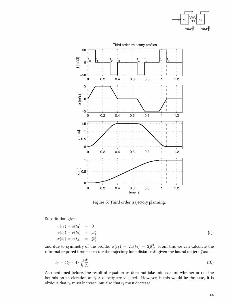
The trajectory planning algorithm will be based on the construction of an appropriate jerkprofile (instead of the acceleration profile as in rigid-body feedforward) that can be integratedthree times to obtain the third order position trajectory. A symmetrical trajectory is completelydetermined by three time intervals: the constant jerk interval t, the constant acceleration intervalta and the constant velocity interval tv. The resulting profiles are given in figure 6. Including thestarting time of the trajectory at t0, there are eight time instances at which the jerk changes. Thefollowing relations are clear:
t = t1 − t0 = t3 − t2 = t5 − t4 = t7 − t6ta = t2 − t1 = t6 − t5tv = t4 − t3
(11)
For step 1 of the algorithm, we will discard the bounds on acceleration and velocity, and onlyconsider the bound on jerk. This implies tv = 0 and ta = 0 and it is clear that this will provideus with a lower bound for the trajectory execution time tx = 4× t.
To obtain t (step 2), we need the relation between t and x with given . For this we make useof the constant value of jerk of + or − during each interval. If we set the time instance of jerkchange to zero, it is easily verified that for any time t during the constant jerk interval the thirdorder profiles for acceleration, velocity and position can be expressed as follows:
a(t) = 0t + a0
v(t) = 120t
2 + a0t + v0
x(t) = 160t
3 + 12a0t
2 + v0t + x0
(12)
Because we assume that the bounds on acceleration and velocity are not violated, we have ta = 0and tv = 0, and consequently from figure 6: t2 = t1 = t and t4 = t3. Hence:
a(t2) = a(t1) = t
v(t2) = v(t1) = 12 t2
x(t2) = x(t1) = 16 t3
(13)
and for the next period in which = −:
a(t4) = a(t3) = −t + a(t2)v(t4) = v(t3) = −1
2 t2 + a(t2)t + v(t2)x(t4) = x(t3) = −1
6 t3 + a(t2)t2 + v(t2)t + x(t2)(14)
13
m 1 m 2
0 0.2 0.4 0.6 0.8 1 1.2−50
0
50Third order trajectory profiles
j [m
/s3] t
0t1
t2
t3
t4
t5
t6
t7
0 0.2 0.4 0.6 0.8 1 1.2−5
0
5
a [m
/s2]
0 0.2 0.4 0.6 0.8 1 1.20
0.5
1
1.5
v [m
/s]
0 0.2 0.4 0.6 0.8 1 1.20
0.5
1
time [s]
x [m
]
Figure 6: Third order trajectory planning.
Substitution gives:
a(t4) = a(t3) = 0v(t4) = v(t3) = t2
x(t4) = x(t3) = t3
(15)
and due to symmetry of the profile: x(t7) = 2x(t3) = 2t3 . From this we can calculate theminimal required time to execute the trajectory for a distance x, given the bound on jerk as:
tx = 4t = 4 · 3
√x
2(16)
As mentioned before, the result of equation 16 does not take into account whether or not thebounds on acceleration and/or velocity are violated. However, if this would be the case, it isobvious that tx must increase, but also that t must decrease.
14
m 1 m 2
Step 3 of the algorithm follows from equation 15; the maximum velocity occurs at t3, suchthat:
v = t2 (17)
If v > v the bound is violated and we must recalculate t as follows:
t =
√v
(18)
Note that the resulting t will always be smaller than the result from equation 16, and that con-sequently also the acceleration (from equation 13) will become smaller. This establishes step 4 ofthe algorithm.
Step 5 follows from equation 13; the maximum acceleration occurs at t1, such that:
a = t (19)
If a > a the bound is violated and we must recalculate t as follows:
t =a
(20)
Again t can only be smaller than previously calculated, such that we now have the guarantee thatt is the maximal value for which none of the bounds is violated. At the same time we have thata maximal value of t will lead to a minimal value of tx and will therefore be (part of) the time-optimal solution. This establishes step 6 of the algorithm and because a is the highest derivativebefore , also step 7.
The next thing to do is to calculate ta: also this value should be maximal for time-optimalperformance, while at the same time it must be such that no bounds are violated. To do thenecessary calculations, assume that ta > 0, such that we now have t2 > t1 (from figure 6).Equation 13 can then be extended with the help of equation 12 and the fact that = 0 during theperiod from t1 to t2:
a(t2) = a(t1) + 0ta = t
v(t2) = v(t1) + a(t1)ta = 12 t2 + tta
x(t2) = x(t1) + v(t1)ta + 12a(t1)t2a
= 16 t3 + 1
2 t2 ta + 12 tt
2a
(21)
Again using equation 12 we can then calculate:
a(t3) = a(t2)− t = 0v(t3) = v(t2) + a(t2)t − 1
2 t2
= 12 t2 + tta + t2 − 1
2 t2
= tta + t2
x(t3) = x(t2) + v(t2)t + 12a(t2)t2 − 1
6 t3
= t3 + 32 t2 ta + 1
2 tt2a
(22)
Now we assume that the velocity bound is not violated, such that t4 = t3. Then due to symmetryof the profile we have:
x(t7) = 2x(t3) = 2t3 + 3t2 ta + tt2a (23)
15
m 1 m 2
By setting x = x(t7) we can then solve ta from the following:
(t) · t2a + (3t2 ) · ta + (2t3 − x) = 0t2a + (3t) · ta + (2t2 − x
t) = 0
(24)
As ta must be positive to make sense, the solution is:
ta = −112 t + 1
2
√9t2 − 8t2 + 4x
t
= −112 t + 1
2
√t2 + 4x
t
(25)
Note that ta >= 0 follows immediately from x >= 2t3 . Hence, we now have determined taunder the assumption that the velocity bound will not be violated: equation 25 establishes steps8 and 9 of the algorithm.
Step 10 introduces the velocity bound again; the maximal velocity is obtained at t3 (see 22):
v = v(t3) = t2 + tta (26)
If v > v the bound is violated and we can recalculate ta as follows:
ta =v − t2
t=
v
t− t =
v
a− t (27)
Now we have determined t and ta to be the time-optimal solution under the restriction of thegiven bounds (step 11).
As the next lower derivative is already v, we can skip step 12 and continue with step 13: thedetermination of the constant velocity time interval tv such that the required total displacementx is obtained. From the previous calculations follows that tv = 0 if ta is according to equation 25.But if ta is reduced according to equation 27, we will have x(t7) < x and we must add a constantvelocity phase to the trajectory such that x(t4)−x(t3) = x−2x(t3). With equation 22 this impliesthat we can calculate tv as:
tv =x− 2t3 − 3t2 ta − tt
2a
v(28)
This completes the calculation of the characteristics of the time-optimal third order profile for agiven distance x and given bounds v, a and . The total displacement x can be expressed as afunction of and the times t, ta and tv:
x = (2t3 + 3t2 ta + tt
2a
)+ v(t3)tv
= (2t3 + 3t2 ta + tt
2a + t2 tv + ttatv
) (29)
16
m 1 m 2
6 Fourth order trajectory planning
This chapter will provide the derivations and calculations necessary to ‘fill in’ the algorithm devel-oped in chapter 4 for fourth order trajectory planning. First the main algorithm will be derived,analogous to the third order algorithm in the previous chapter. Section 6.2 will then give thederivation of the solution of the third order polynomial equation that will appear in one of thesteps of this main algorithm.
6.1 Main algorithm
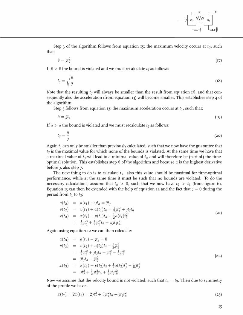
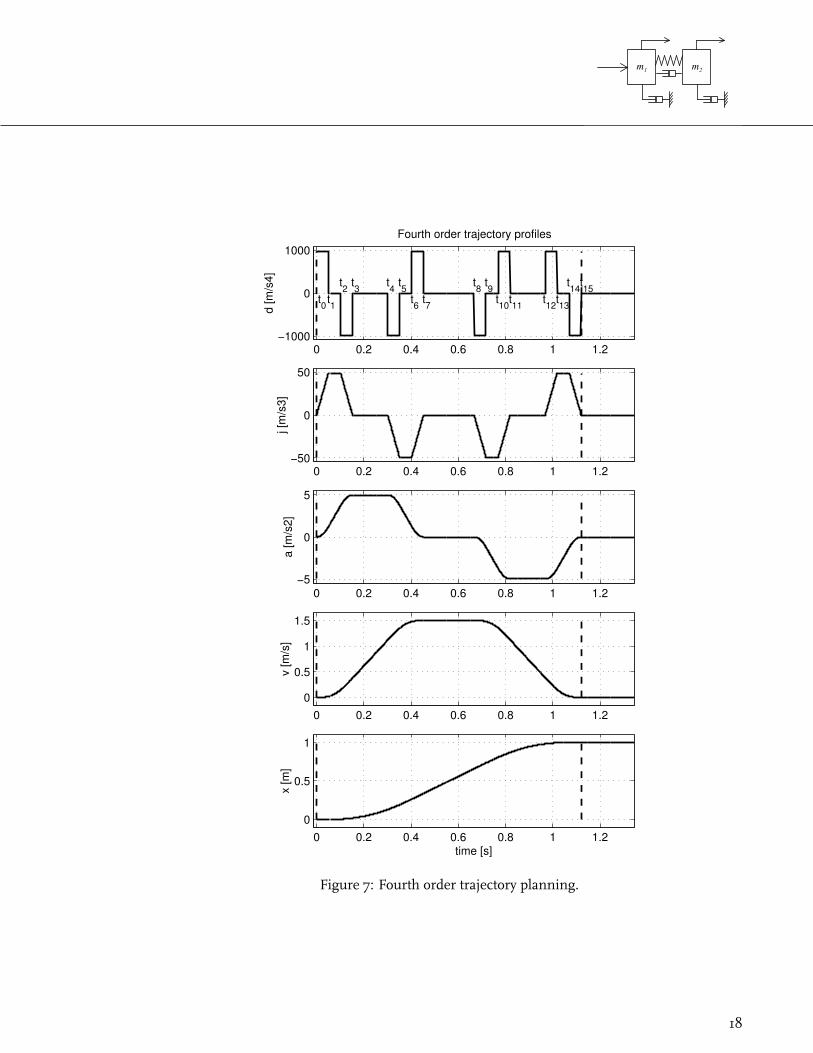
Again we will assume that a symmetrical trajectory must be planned for a point to point moveover a distance x. We have bounds on velocity (v), acceleration (a), jerk () and derivative of jerk(d). The trajectory planning algorithm will now be based on the construction of a derivative ofjerk profile that can be integrated four times to obtain the fourth order position trajectory. Asymmetrical trajectory is completely determined by four time intervals: the constant derivative ofjerk interval td, the constant jerk interval t, the constant acceleration interval ta and the constantvelocity interval tv. The resulting profiles are given in figure 7.
Including the starting time of the trajectory at t0, there are now sixteen time instances atwhich the derivative of jerk changes.
For step 1 of the algorithm, we will discard the bounds on jerk, acceleration and velocity, andonly consider the bound on the derivative of jerk. This implies tv = 0, ta = 0 and t = 0 and it isclear that this will provide us with a lower bound for the trajectory execution time tx = 8× td.
To obtain td (step 2), we need the relation between td and x with given d. For this we makeuse of the constant value of derivative of jerk of +d or −d during each interval. If we set thetime instance of derivative of jerk change to 0, it is easily verified that for any time t during theconstant derivative of jerk interval the fourth order profiles for acceleration, velocity and positioncan be expressed as follows:
(t) = d0t + 0
a(t) = 12d0t
2 + 0t + a0
v(t) = 16d0t
3 + 120t
2 + a0t + v0
x(t) = 124d0t
4 + 160t
3 + a0t2 + v0t + x0
(30)
Because we assume that the bounds on jerk, acceleration and velocity are not violated, we havet = 0, ta = 0 and tv = 0, and consequently from figure 7: t2 = t1 = td, t4 = t3 = 2td,t6 = t5 = 3td and t8 = t7 = 4td. Hence:
(t1) = dtda(t1) = 1
2 dt2d
v(t1) = 16 dt3
d
x(t1) = 124 dt4
d
(31)
17
m 1 m 2
0 0.2 0.4 0.6 0.8 1 1.2−1000
0
1000Fourth order trajectory profiles
d [m
/s4]
t0t1
t2
t3
t4
t5
t6
t7
t8
t9
t10
t11
t12
t13
t14
t15
0 0.2 0.4 0.6 0.8 1 1.2−50
0
50
j [m
/s3]
0 0.2 0.4 0.6 0.8 1 1.2−5
0
5
a [m
/s2]
0 0.2 0.4 0.6 0.8 1 1.20
0.5
1
1.5
v [m
/s]
0 0.2 0.4 0.6 0.8 1 1.20
0.5
1
time [s]
x [m
]
Figure 7: Fourth order trajectory planning.
18
m 1 m 2
and for the next period in which d = −d:
(t3) = −dtd + (t2)a(t3) = −1
2 dt2d
+ (t2)td + a(t2)
v(t3) = −16 dt3
d+ 1
2(t2)t2d + a(t2)td + v(t2)
x(t3) = − 124 dt4
d+ 1
6(t2)t3d + 12a(t2)t2d + v(t2)td + x(t2)
(32)
Substitution gives:
(t3) = 0a(t3) = dt2
d
v(t3) = dt3d
x(t3) = 712 dt4
d
(33)
Again using equation 30, we can calculate the results of the subsequent periods as:
(t5) = −dtda(t5) = 1
2 dt2d
v(t5) = 156 dt3
d
x(t5) = 2 124 dt4
d
(34)
and:
(t7) = 0a(t7) = 0v(t7) = 2dt3
d
x(t7) = 4dt4d
(35)
and due to symmetry of the profile: x(t15) = 2x(t7) = 8dt4d. From this we can calculate td as
required by steps 1 and 2 of the trajectory planning algorithm as:
td = 4
√x
8d(36)
To continue with step 3 we have that the maximal velocity is obtained at time instance t7. Hence,from equation 35 follows:
v = v(t7) = 2dt3d (37)
If v > v we must recalculate td as:
td = 3
√v
2d(38)
which establishes step 4. Next, step 5 follows from the calculation of maximal acceleration ob-tained at time instance t3. From equation 33 we have:
a = a(t3) = dt2d (39)
and if a > a we must recalculate td as:
td =√
a
d(40)
19
m 1 m 2
which establishes step 6. In this case we have one further test (step 7) to do on the maximal jerkobtained at t1:
= (t1) = dtd (41)
and if > we must recalculate td as:
td =
d(42)
Hence, we now have a value for td that complies with all of the bounds , a and v.The next thing to do is to calculate t under the assumption that bounds a and v are not
violated (steps 8 and 9). To do the necessary calculations, assume that t > 0, such that we nowhave t2 > t1 and t6 > t5 (from figure 7). Equation 30 and the fact that d = 0 during the periodfrom t1 to t2 now enables us to calculate:
(t2) = dtda(t2) = 1
2 dt2d
+ dtdt
v(t2) = 16 dt3
d+ 1
2 dt2dt + 1
2 dtdt2
x(t2) = 124 dt4
d+ 1
6 dt3dt + 1
4 dt2dt2 + 1
6 dtdt3
(43)
Again using equation 30 we can then calculate:
(t3) = 0a(t3) = dt2
d+ dtdt
v(t3) = dt3d
+ 112 dt2
dt + 1
2 dtdt2
x(t3) = 712 dt4
d+ 11
6 dt3dt + 3
4 dt2dt2 + 1
6 dtdt3
(44)
(t5) = −dtda(t5) = 1
2 dt2d
+ dtdt
v(t5) = 156 dt3
d+ 21
2 dt2dt + 1
2 dtdt2
x(t5) = 2 124 dt4
d+ 31
6 dt3dt + 11
4 dt2dt2 + 1
6 dtdt3
(45)
(t6) = −dtda(t6) = 1
2 dt2d
v(t6) = 156 dt3
d+ 3dt2
dt + dtdt
2
x(t6) = 2 124 dt4
d+ 5dt3
dt + 4dt2
dt2 + dtdt
3
(46)
(t7) = 0a(t7) = 0v(t7) = 2dt3
d+ 3dt2
dt + dtdt
2
x(t7) = 4dt4d
+ 8dt3dt + 5dt2
dt2 + dtdt
3
(47)
Now with t8 = t7 and due to symmetry of the profile we have:
x(t15) = 2x(t7) = 8dt4d + 16dt3dt + 10dt2dt2 + 2dtdt
3 (48)
20
m 1 m 2
By setting x = x(t15) we can then solve t from the following:
(2dtd)t3 + (10dt2
d)t2 + (16dt3
d)t + (8dt4
d− x) = 0
⇒ t3 + (5td)t2 + (8t2
d)t + (4t3
d− x
2dtd) = 0
(49)
The derivation of the solution of this third order polynomial equation is given in section 6.2.There it will be proven that there always exists a positive (or zero) real solution:
p := −19 t2
d
q := − 127 t3
d− x
4dtd
D := p3 + q2
r := 3√−q +
√D
t = r − pr −
53 td
(50)
After this, step 10 introduces the velocity and acceleration bounds again; the maximal velocity isobtained at t7 (see 47):
v = v(t7) = 2dt3d + 3dt2dt + dtdt2 (51)
If v > v the bound is violated and we can recalculate t from the second order polynomial:
t2 + 3tdt + 2t2d −v
dtd= 0 (52)
The positive real solution for this is:
t = −112td +
√√√√ t2d
4+
v
dtd(53)
Next, the maximal acceleration is obtained at t3 (see 44):
a = a(t3) = dt2d + dtdt (54)
If a > a we can recalculate t as:
t =a
− td (55)
and we arrive at step 11 of the planning algorithm.In accordance with step 12 there is one further extension of the trajectory required for the
calculation of ta. To do the necessary calculations, assume that ta > 0, such that we now havet4 > t3 (from figure 7). Equation 30 and the fact that d = 0 and = 0 during the period from t3to t4 now enables us to calculate:
(t4) = 0a(t4) = dt2
d+ dtdt
v(t4) = dt3d
+ 112 dt2
dt + 1
2 dtdt2 + dt2
dta + dtdtta
x(t4) = 712 dt4
d+ 11
6 dt3dt + 3
4 dt2dt2 + 1
6 dtdt3+
12 dt2
dt2a + 1
2 dtdtt2a + dt3
dta + 11
2 dt2dtta+
12 dtdt
2 ta
(56)
21
m 1 m 2
(t5) = −dtda(t5) = 1
2 dt2d
+ dtdt
v(t5) = 156 dt3
d+ 21
2 dt2dt + 1
2 dtdt2 + dt2
dta + dtdtta
x(t5) = 2 124 dt4
d+ 31
6 dt3dt + 11
4 dt2dt2 + 1
6 dtdt3+
12 dt2
dt2a + 1
2 dtdtt2a + 2dt3
dta + 21
2 dt2dtta+
12 dtdt
2 ta
(57)
(t6) = −dtda(t6) = 1
2 dt2d
v(t6) = 156 dt3
d+ 3dt2
dt + dtdt
2 + dt2
dta + dtdtta
x(t6) = 2 124 dt4
d+ 5dt3
dt + 4dt2
dt2 + dtdt
3+
12 dt2
dt2a + 1
2 dtdtt2a + 2dt3
dta + 31
2 dt2dtta+
112 dtdt
2 ta
(58)
(t7) = 0a(t7) = 1
2 dt2d
v(t7) = 2dt3d
+ 3dt2dt + dtdt
2 + dt2
dta + dtdtta
x(t7) = 4dt4d
+ 8dt3dt + 5dt2
dt2 + dtdt
3+
12 dt2
dt2a + 1
2 dtdtt2a + 3dt3
dta + 41
2 dt2dtta+
112 dtdt
2 ta
(59)
Now, given that td and t are already determined and the planned trajectory is symmetrical, wecan solve ta such that x(t15) = 2x(t7) = x from the following polynomial equation:
{dt2d
+ dtdt}t2a + {6dt3d
+ 9dt2dt + 3dtdt
2}ta+
{8dt4d
+ 16dt3dt + 10dt2
dt2 + 2dtdt
3 − x} = 0
(60)
Clearly ta must be the positive root of this second order polynomial (compare with equation 25).Now we can introduce the velocity bound again; the maximal velocity is obtained at t7 (see
59):
v = 2dt3d + 3dt2dt + dtdt2 + dt2dta + dtdtta (61)
If v > v the bound is violated and we can recalculate ta as:
ta =v − 2dt3
d− 3dt2
dt − dtdt
2
dt2d
+ dtdt(62)
Now we have determined td, t and ta under the restriction of the given bounds and, as the nextderivative is v, this establishes step 12 of the algorithm.
Finally, step 13 will determine the constant velocity time interval tv such that the required totaldisplacement x is obtained. From the previous calculations follows that tv = 0 if ta is accordingto equation 60. But if ta is reduced according to equation 62, we will have x(t15) < x and wemust add a constant velocity phase to the trajectory such that x(t4) − x(t3) = x − 2x(t7). Withequation 59 this implies that we can calculate tv as:
tv =x− 2x(t7)
v(63)
22
m 1 m 2
This completes the calculation of the characteristics of the symmetrical fourth order profile for agiven distance x and given bounds v, a, and d. We can further state that if the trajectory containsa constant velocity phase (i.e. tv > 0), the trajectory is time-optimal. The total displacement x canbe expressed as a function of d and the times td t, ta and tv:
x = d ( t2dt2a + tdtt
2a + 6t3
dta + 9t2
dtta + 3tdt
2 ta+
8t4d
+ 16t3dt + 10t2
dt2 + 2tdt
3 + 2t3
dtv+
3t2dttv + tdt
2 tv + t2
dtatv + tdttatv )
(64)
6.2 Solution of equation 49
A solution of the third order polynomial equation 49 is a valid solution t if and only if the solutionis real and larger than or equal to zero. This section will consider the existence of such a solutionand derive its calculation. The results of this section are based on Cardan’s formula, as can forinstance be found in [2].
Given a third order polynomial equation (also known as a cubic equation) in variable x of theform:
x3 + ax2 + bx + c = 0 (65)
with constant real parameters a, b and c. This can be rewritten as:
y3 + 3py + 2q = 0 (66)
with new variable y defined as:
y = x + 13a (67)
and new parameters p and q defined as:
p = 13b− 1
9a2
q = 127a3 − 1
6ab + 12c
(68)
Applying this to equation 49 gives:
p = 83 t2
d− 25
9 t2d
= −19 t2
d
q = 12527 t3
d− 40
6 t3d
+ 2t3d− x
4dtd= − 1
27 t3d− x
4dtd
(69)
From [2] we have that the characteristics of the solution are determined by the sign of the dis-criminant D:
D = p3 + q2 = (−19 t2
d)3 + (− 1
27 t3d− x
4dtd)2
= − 1729
t6d +1
729t6d︸ ︷︷ ︸
=0
+xt2
d
54d+
x2
16d2t2d︸ ︷︷ ︸
>0
> 0 (70)
Now D > 0 implies that there exists one real and two complex conjugated solutions, and onlythe real solution is a valid candidate for t. Based on Cardan’s formula for equation 67 the realsolution can be found from:
y = 3√−q +
√D + 3
√−q −
√D (71)
23
m 1 m 2
such that:
x = y − 13a ⇒ t = y − 5
3 td (72)
Next, to prove that this real solution must also be larger than or equal to zero, consider the signsof the coefficients of equation 49:
a = 5td > 0b = 8t2
d> 0
c = 4t3d− x
2dtd≤ 0
(73)
Now consider the function f(x) = x3 + ax2 + bx + c. Obviously, if c = 0 the solution is x = 0(i.e. t = 0). If c < 0, we have f(0) = c < 0 and f(x) is monotone increasing for x ≥ 0 andlimx→∞ f(x) = ∞. Hence, the function f(x) must cross the positive real axis, thus establishinga positive real solution. This solution must be given by equations 71 and 72, as this is the onlyreal solution.
For easier implementation of this solution, equations 71 and 72 are simplified as follows:
t = 3√−q +
√D + 3
√−q −
√D − 5
3 td
= 3√−q +
√D +
3√−q+
√D
3√−q−
√D
3√−q+
√D
− 53 td
= 3√−q +
√D +
3√−q2−D
3√−q+
√D− 5
3 td
= 3√−q +
√D − p
3√−q+
√D− 5
3 td
(74)
With this result it is not necessary to calculate the second term: 3√−q −
√D, which saves time
and also has a positive effect on accuracy of finite precision calculations.
24

m 1 m 2
7 Implementation aspects
7.1 Switching times
From the previous chapters it is clear that the derivations for especially fourth order trajectoryplanning are quite elaborate. However, the calculations actually required for implementation ofthis planner are relatively straightforward. The algorithm of chapter 4 consists of a combinationof polynomial calculations with simple if-then-else tests for which most state-of-the-art motioncontrol hardware has standard algorithms.
When considering implementation of the planned trajectory into a feedforward control scheme,it is important to consider the effect of discretization. This implies that the integrators and thefeedforward filter as given in the diagram of figure 5 will all have to be implemented in discretetime at some given sampling time interval Ts. This also implies that the switching time instancesof the planned trajectory must be synchronized with the sampling time instances: i.e. the timeintervals tv, ta, etc. must be multiples of Ts.
To obtain this, it must be accepted that time-optimality as resulting from the continuous timecalculations in the previous chapters is lost. The calculated time intervals must be rounded-offtowards a multiple of Ts. This must be done such that the given bounds are not violated, but atthe same time approximated as closely as possible. The approach proposed here is to extend thealgorithm of chapter 4. After each calculation or re-calculation of a time interval, the result isrounded-off upward to the next multiple of Ts. Next the maximal value of the highest derivativeis calculated accordingly.
As an example consider the first calculation of td for a fourth order trajectory (equation 36).The rounded-off value for td can be calculated as:
t′d = ceil(
tdTs
)× Ts (75)
with ceil(.) denoting the rounding off towards the next higher integer. From equation 36 we canthen calculate a new value for d:
d′ =x
8t′d4 (76)
Note that with t′d≥ td we must have d′ ≤ d.
It can be verified that this same approach is valid for the calculation or re-calculation of alltime intervals. It is important to note that with each new calculation of d′ its value must reduce.This guarantees that none of the bounds that were checked in earlier steps of the algorithm willbe violated.
State-of-the-art motion controllers are equipped with a high resolution floating point calculationunit, such that quantization effects are usually negligible. To check this, we canmake use of equa-tion 64 to calculate the obtained position in case a quantized d′ is used. The difference betweendesired position and calculated position can be accounted for by means of a correction signal onthe position trajectory. Typically in a digital system, the position signal is also quantized (usuallyin encoder increments). The correction signal can then be implemented by adding some incre-ments to the position reference at each sampling instance during the trajectory. In relevant casesonly one or two correction increments at each sampling instance should be sufficient (to preventdeterioration of the feedforward control). In case larger corrections are necessary, the accuracyand/or sampling rate of the motion control hardware should be increased.
25
m 1 m 2
A complete algorithm for fourth order trajectory planning is given in the appendix. This algo-rithm is given as a Matlab .M function, which calculates the times td t, ta and tv. It also includesthe possibility to specify a sampling time interval. It then uses equations 75 and 76 to synchronizethe switching time instances with the sampling time instances and to calculate d′. Finally, it al-lows compensation for the effect of quantization by specifying a number of significant decimalsfor d′ and calculating the required amount of correction increments for the position referencesignal.
7.2 Synchronization of profiles
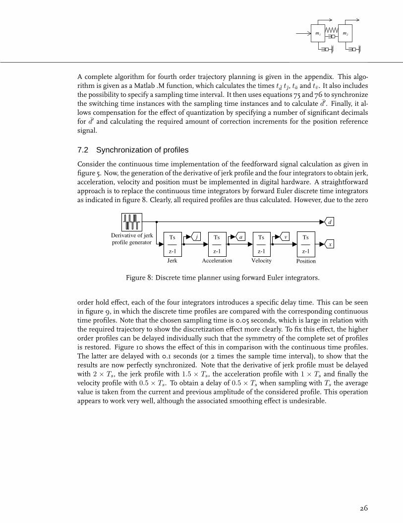
Consider the continuous time implementation of the feedforward signal calculation as given infigure 5. Now, the generation of the derivative of jerk profile and the four integrators to obtain jerk,acceleration, velocity and position must be implemented in digital hardware. A straightforwardapproach is to replace the continuous time integrators by forward Euler discrete time integratorsas indicated in figure 8. Clearly, all required profiles are thus calculated. However, due to the zero
Ts-----z-1----
Velocity
Ts-----z-1----
Position
Ts-----z-1----
Jerk
xva
d
jDerivative of jerkprofile generator
Ts-----z-1----
Acceleration
Figure 8: Discrete time planner using forward Euler integrators.
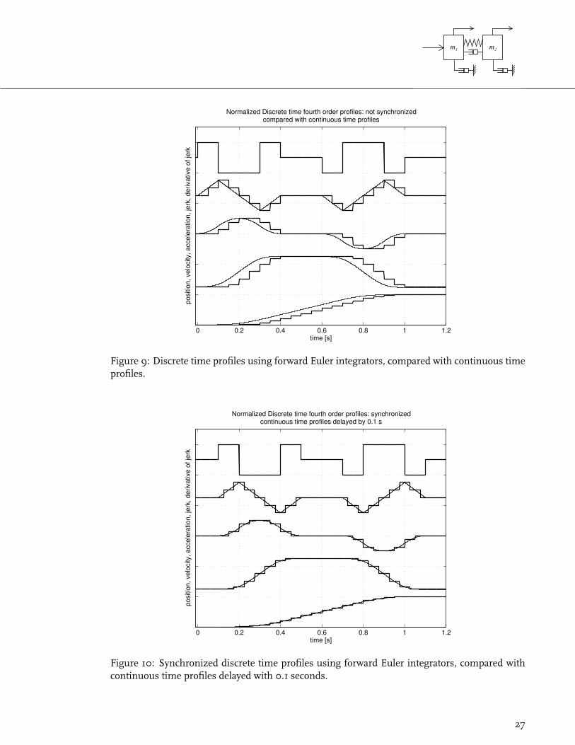
order hold effect, each of the four integrators introduces a specific delay time. This can be seenin figure 9, in which the discrete time profiles are compared with the corresponding continuoustime profiles. Note that the chosen sampling time is 0.05 seconds, which is large in relation withthe required trajectory to show the discretization effect more clearly. To fix this effect, the higherorder profiles can be delayed individually such that the symmetry of the complete set of profilesis restored. Figure 10 shows the effect of this in comparison with the continuous time profiles.The latter are delayed with 0.1 seconds (or 2 times the sample time interval), to show that theresults are now perfectly synchronized. Note that the derivative of jerk profile must be delayedwith 2 × Ts, the jerk profile with 1.5 × Ts, the acceleration profile with 1 × Ts and finally thevelocity profile with 0.5 × Ts. To obtain a delay of 0.5 × Ts when sampling with Ts the averagevalue is taken from the current and previous amplitude of the considered profile. This operationappears to work very well, although the associated smoothing effect is undesirable.
26
m 1 m 2
0 0.2 0.4 0.6 0.8 1 1.2
Normalized Discrete time fourth order profiles: not synchronizedcompared with continuous time profiles
time [s]
posi
tion,
vel
ocity
, acc
eler
atio
n, je
rk, d
eriv
ativ
e of
jerk
Figure 9: Discrete time profiles using forward Euler integrators, compared with continuous timeprofiles.
0 0.2 0.4 0.6 0.8 1 1.2
Normalized Discrete time fourth order profiles: synchronizedcontinuous time profiles delayed by 0.1 s
time [s]
posi
tion,
vel
ocity
, acc
eler
atio
n, je
rk, d
eriv
ativ
e of
jerk
Figure 10: Synchronized discrete time profiles using forward Euler integrators, compared withcontinuous time profiles delayed with 0.1 seconds.
27
m 1 m 2
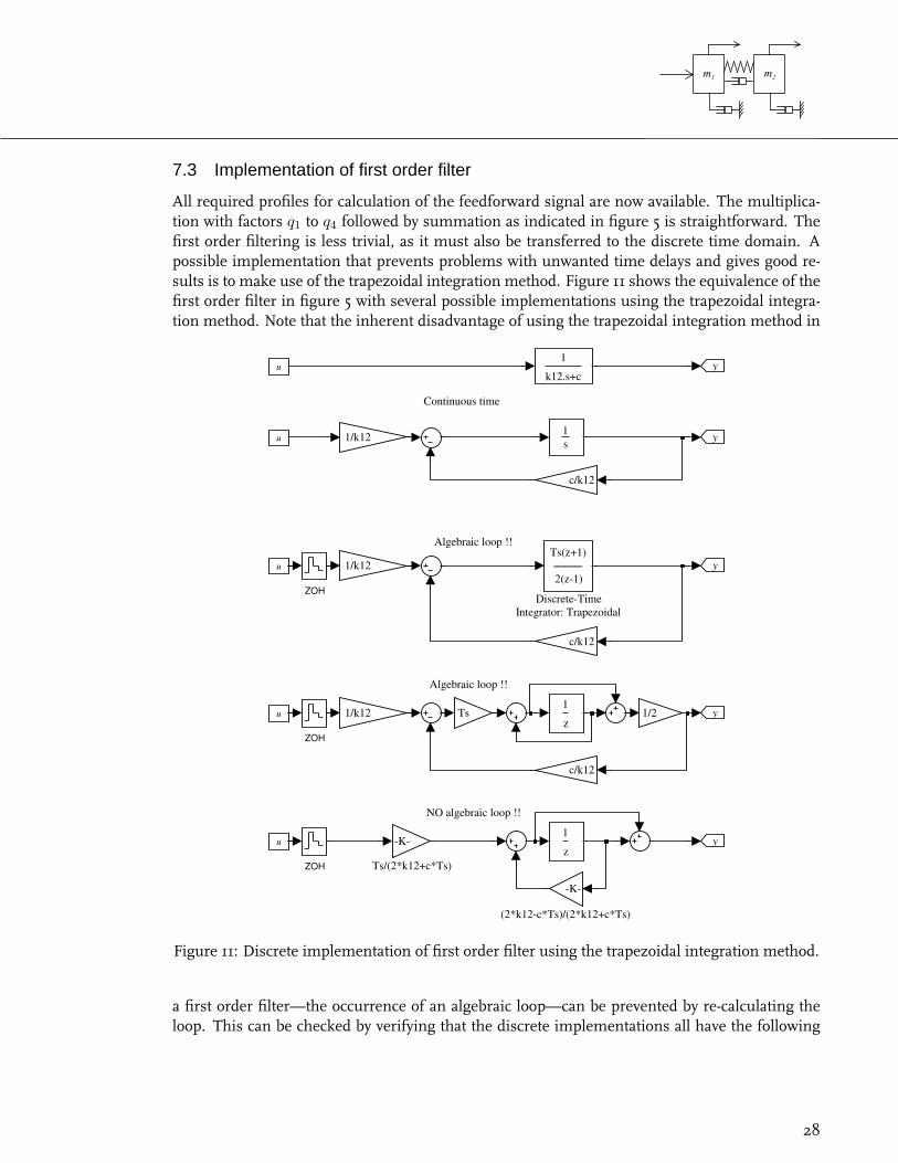
7.3 Implementation of first order filter
All required profiles for calculation of the feedforward signal are now available. The multiplica-tion with factors q1 to q4 followed by summation as indicated in figure 5 is straightforward. Thefirst order filtering is less trivial, as it must also be transferred to the discrete time domain. Apossible implementation that prevents problems with unwanted time delays and gives good re-sults is to make use of the trapezoidal integration method. Figure 11 shows the equivalence of thefirst order filter in figure 5 with several possible implementations using the trapezoidal integra-tion method. Note that the inherent disadvantage of using the trapezoidal integration method in
Algebraic loop !!
Algebraic loop !!
NO algebraic loop !!
Continuous time
ZOH
ZOH
ZOH
y
y
y
y
y
c/k12
c/k12
c/k12
z
1
z
11/2Ts
-K-
Ts/(2*k12+c*Ts)
1
k12.s+c
1s
Ts(z+1)--------2(z-1)-------
Discrete-TimeIntegrator: Trapezoidal
u
u
u
u
u
1/k12
1/k12
1/k12
-K-
(2*k12-c*Ts)/(2*k12+c*Ts)
Figure 11: Discrete implementation of first order filter using the trapezoidal integration method.
a first order filter—the occurrence of an algebraic loop—can be prevented by re-calculating theloop. This can be checked by verifying that the discrete implementations all have the following
28
m 1 m 2
transfer function:
y =Ts
2k12+cTs(z + 1)
z − 2k12−cTs2k12+cTs
u (77)
7.4 Calculation of reference trajectory
A final point on synchronization must be made with respect to the calculation of the referencetrajectory that is used for feedback control. When applying the feedforward signal as calculatedabove, based on the synchronized profiles as illustrated in figure 10, the actual plant’s responsewill be close to the ideal continuous time response with a delay of 2 × Ts. However, in orderto compare this signal with the reference trajectory it must be sampled with the same samplingfrequency as is used for generation of the reference trajectory. The sample and hold device usedfor this will then introduce an average delay of exactly 0.5× Ts.
Hence, to compensate for this further delay, it is necessary to also delay the reference tra-jectory with this same value. This additional delay can be implemented in the same manner asmentioned before: by taking the average between the current and previous reference trajectoryvalue. The result of this will be that the control error will not be affected by sampling. The con-troller will only act on the effects of disturbances and on discrepancies between the actual plantand the modelled fourth order behavior.
Obviously, this is only true if the sampling frequency is sufficiently high: otherwise the mo-mentary control error may deviate significantly from the average value. If this is the case, anincrease in sampling frequency must be considered. Usually however, the sampling frequencyis more significantly determined by the demands on stability and performance of the (digital)feedback controller.
29
m 1 m 2
8 Simulation results
A theoretical motivation for the application of fourth order feedforward as an extension of rigidbody feedforward was already given in chapter 3. Next, subsequent chapters have shown thatfourth order feedforward is feasible in the sense of trajectory planning and (digital) feedforwardimplementation. This chapter will give further motivation for application of fourth order feedfor-ward by considering some simulation results.
The main concern when considering model based feedforward control is the occurrence ofdiscrepancies between the behavior of the actual motion system and the used model. This oftenmotivates the use of rigid body feedforward, as the total mass of the motion system is usuallyknown within tight boundaries. Furthermore, a well designed motion system will have limitedfriction and damping: especially dry friction must be minimized as it leads to classical problemsin both feedforward and feedback. Linear viscous damping can more easily be dealt with, butoften shows time dependent behavior: if damping has a reasonably constant value, it can be com-pensated as shown in chapter 2. Now, fourth order feedforward introduces several additionalphysical parameters that may, or may not be constant: a mass ratio (division of mass in m1 andm2), a damping ratio (division of damping in k1 and k2), a spring stiffness c and an internaldamping k12 (see figures 1 and 4). The simulation results in this chapter will show that fourthorder feedforward will give a significant improvement of performance (in the sense of servo er-rors during or after trajectory execution) in comparison with rigid body feedback, even if theseadditional parameters have relatively large uncertainties.
All simulations will be performed using the configuration of figure 5. The motion systemparameters and their variations used in the simulations are given in table 1 The trajectory pa-
Parameter Value Unit Variationm1 20 Kg m1 ∈ {15 · · · 25},m2 10 Kg m2 = 30−m1
k1 10 Ns/m k1 ∈ {5 · · · 15},k2 10 Ns/m k2 = 20− k1
c 6 · 105 N/m ±33%k12 500 Ns/m ±100%
Table 1: Simulation parameters
rameters are defined in table 2. When comparing with rigid body feedforward, the fourth order
Parameter Symbol Value Unitderivative of jerk d 1000 m/s4
jerk 50 m/s3
acceleration a 5 m/s2
velocity v 1 m/sdisplacement x 1 m
Table 2: Trajectory definition parameters
trajectory will be used, such that the smoothing effect of using a high order trajectory is notaccountable for the difference. In that case, it can easily be verified that optimal rigid body feed-forward is obtained by setting m1 = 30, m2 = 0, k1 = 20, k2 = 0 and k12 = 0. From
30
m 1 m 2
equation 9 we then have q1 = q2 = 0, q3 = m1c and q4 = k1c. Furthermore, the first orderfilter reverts to a constant gain of 1
c (see also equation 77) and equation 10 reverts to equation 1.Note that the value of c becomes unimportant as it drops out of the calculations. To remove theeffect of feedback control from the results, most simulations are performed in open loop.
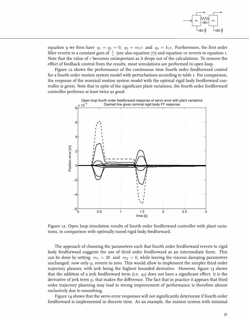
Figure 12 shows the performance of the continuous time fourth order feedforward controlfor a fourth order motion system model with perturbations according to table 1. For comparison,the response of the nominal motion system model with the optimal rigid body feedforward con-troller is given. Note that in spite of the significant plant variations, the fourth order feedforwardcontroller performs at least twice as good.
0 0.5 1 1.5 2 2.5 3−6
−4
−2
0
2
4
6
8x 10⁻⁵
Open loop fourth order feedforward response of servo error with plant variationsDashed line gives nominal rigid body FF response
time [s]
Pos
ition
err
or [m
]
Figure 12: Open loop simulation results of fourth order feedforward controller with plant varia-tions, in comparison with optimally tuned rigid body feedforward.
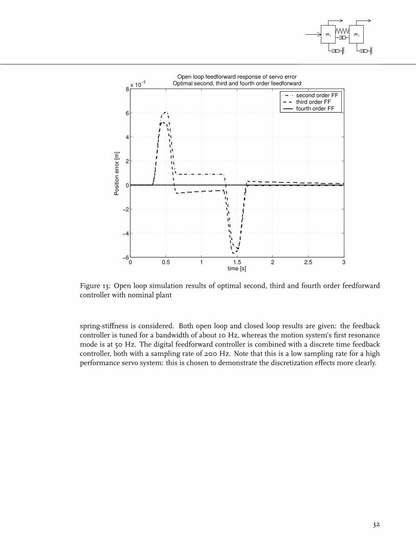
The approach of choosing the parameters such that fourth order feedforward reverts to rigidbody feedforward suggests the use of third order feedforward as an intermediate form. Thiscan be done by setting m1 = 30 and m2 = 0, while leaving the viscous damping parametersunchanged: now only q1 reverts to zero. This would allow to implement the simpler third ordertrajectory planner, with jerk being the highest bounded derivative. However, figure 13 showsthat the addition of a jerk feedforward term (i.e. q2) does not have a significant effect: it is thederivative of jerk term q1 that makes the difference. The fact that in practice it appears that thirdorder trajectory planning may lead to strong improvement of performance is therefore almostexclusively due to smoothing.
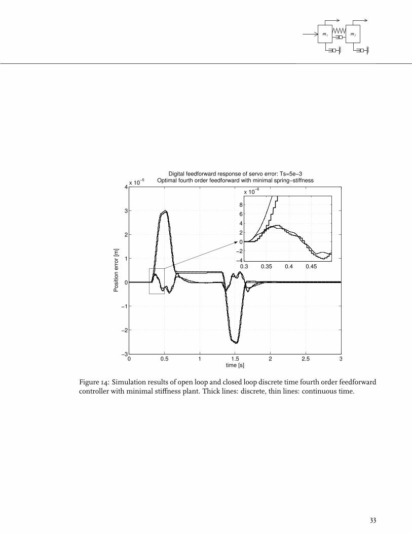
Figure 14 shows that the servo error responses will not significantly deteriorate if fourth orderfeedforward is implemented in discrete time. As an example, the motion system with minimal
31
m 1 m 2
0 0.5 1 1.5 2 2.5 3−6
−4
−2
0
2
4
6
8x 10⁻⁵
Open loop feedforward response of servo errorOptimal second, third and fourth order feedforward
time [s]
Pos
ition
err
or [m
]
second order FFthird order FFfourth order FF
Figure 13: Open loop simulation results of optimal second, third and fourth order feedforwardcontroller with nominal plant
spring-stiffness is considered. Both open loop and closed loop results are given: the feedbackcontroller is tuned for a bandwidth of about 10 Hz, whereas the motion system’s first resonancemode is at 50 Hz. The digital feedforward controller is combined with a discrete time feedbackcontroller, both with a sampling rate of 200 Hz. Note that this is a low sampling rate for a highperformance servo system: this is chosen to demonstrate the discretization effects more clearly.
32
m 1 m 2
0 0.5 1 1.5 2 2.5 3−3
−2
−1
0
1
2
3
4x 10⁻⁵
time [s]
Pos
ition
err
or [m
]
Digital feedforward response of servo error: Ts=5e−3Optimal fourth order feedforward with minimal spring−stiffness
0.3 0.35 0.4 0.45−4
−2
0
2
4
6
8
x 10−6
Figure 14: Simulation results of open loop and closed loop discrete time fourth order feedforwardcontroller with minimal stiffness plant. Thick lines: discrete, thin lines: continuous time.
33
m 1 m 2
9 Conclusions
For high performance motion control, especially for electromechanical motion systems, the use-fulness of feedforward control is well known and often implemented. This report shows thatthe popular simple feedforward scheme known as ‘mass-feedforward’, ‘rigid-body feedforward’or ‘second-order feedforward’ can be extended to higher order feedforward while still maintain-ing important practical properties like time-optimality, actuator effort limitation, reliability, im-plementability and accuracy. Furthermore, it is argumented that the increase in complexity ismanageable in state-of-the-art motion control hardware.
Third order feedforward, which is increasingly applied in practice, appears to be mainly ef-fective due to ‘smoothing’ of the trajectory, i.e. reduction of the high frequency content of thetrajectory, such that feedback control can be more effective. The use of fourth order feedforwardfor high performance electromechanical motion systems is motivated by considering an appro-priate model and supported by simulation results. Apart from the mentioned smoothing effect,the feedforward of the derivative of jerk profile appears to result in a significant performanceimprovement. This is even more remarkable when considering that, for relevant cases, the cal-culated feedforward force is hardly affected.
A high level algorithm is given to calculate higher order trajectories for point-to-point moves;other motion commands, like speed change operations, can be derived from this. For third andfourth order trajectory planning, the details of the algorithm are worked out, resulting in practical,reliable and accurate algorithms.
Further implementation issues, like discrete time calculations, quantization effects and syn-chronization, are explicitly addressed. The trajectory planning algorithms can be implementedsuch that switching times are exactly synchronized with sampling instances. A digital implemen-tation is suggested that takes care of the synchronization of the various profiles with each otherand the position trajectory, and also with the measured position. It is shown that deteriorationof the continuous time results due to sampling are small when applying a sufficient samplingrate. Experience shows that a sampling rate that is required for stable feedback control is alsosufficient for feedforward control.
Simulation results show that the improvement obtained with fourth order feedforward is notoverly sensitive to variations in the parameters that are additional to the ‘classic’ parameters ofrigid-body feedforward (i.e. mass and viscous damping). Obviously, the feedforward performancewill improve if the dynamical behavior of the actual motion system is closer to that of the fourthorder model and said parameters are known within tighter bounds. An important advantage ofthe suggested implementation is the possibility to manually fine-tune the feedforward amplifica-tion factor for each profile (the q factors). This can be seen as a simple, direct extension of thewell known practice of fine-tuning rigid-body feedforward.
34
m 1 m 2
References
[1] M. Boerlage, M. Steinbuch, P. Lambrechts, M. van de Wal, ‘Model based feedforward formotion systems’. Submitted, 2003.
[2] I.N. Bronshtein, K.A. Semendyayev, ‘A ’Guide book to mathematics’. Verlag Harri Deutsch,Frankfurt, ISBN 3-87144-095-7, 1973.
[3] S. Devasia, ‘Robust inversion-based feedforward controllers for output tracking under plantuncertainty’. Proc. of the American Control Conference, 2000, pp.497-502.
[4] B.G. Dijkstra, N.J. Rambaratsingh, C. Scherer, O.H. Bosgra, M. Steinbuch, S. Kerssemakers,‘Input design for optimal discrete-time point-to-point motion of an industrial XY positioningtable’, in Proc. 39th IEEE Conference on Decision and Control, 2000, pp.901-906.
[5] L. Hunt, G. Meyer, ‘Noncausal inverses for linear systems’. IEEE Trans. on Automatic Control,1996, Vol. 41(4), pp.608-611.
[6] P.H. Meckl, ‘Discussion on: comparison of filtering methods for reducing residual vibra-tion’. European Journal of Control, 1999, Vol. 5, pp.219-221.
[7] P.H. Meckl, P.B. Arestides, M.C. Woods, ‘Optimized S-curve motion profiles for minimumresidual vibration’. Proc. of the American Control Conference, 1998, pp.2627-2631.
[8] B.R. Murphy, I. Watanaabe, ‘Digital shaping filters for reducing machine vibration’. IEEETrans. on Robotics and Automation, 1992, Vol. 8(2), pp.285-289.
[9] F. Paganini, A. Giusto, ‘Robust synthesis of dynamic prefilters’, Proc. of the American ControlConference, 1997, pp.1314-1318.
[10] H. S. Park, P.H. Chang, D.Y. Lee, ‘Concurrent design of continuous zero phase error track-ing controller and sinusoidal trajectory for improved tracking control’. J. Dynamic Systems,Measurement, and Control, 2001, Vol. 5, pp.3554-3558.
[11] D. Roover, ‘Motion control for a wafer stage’, Delft University Press, The Netherlands, 1997.
[12] D. Roover, F. Sperling, ‘Point-to-point control of a high accuracy positioning mechanism’,Proc. of the American Control Conference, 1997, pp.1350-1354.
[13] N. Singer, W. Singhose, W. Seering, ‘Comparison of filtering methods for reducing residualvibration’. European Journal of Control, 1999, Vol.5, pp.208-218.
[14] M. Steinbuch, M.L. Norg, ‘Advanced motion control: an industrial perspective’, EuropeanJournal of Control, 1998, pp.278-293.
[15] M. Tomizuka, ‘Zero phase error tracking algorithm for digital control’. J. Dynamic Systems,Measurement, and Control, 1987, Vol.109, pp.65-68.
[16] D.E. Torfs, J. Swevers, J. De Schutter, ‘Quasi-perfect tracking control of non-minimal phasesystems’. Proc. of the 30th Conference on Decision and Control, 1991, pp.241-244.
[17] D.E. Torfs, R. Vuerinckx, J. Swevers, J. Schoukens, ‘Comparison of two feedforward designmethods aiming at accurate trajectory tracking of the end point of a flexible robot arm’, IEEETrans. on Control Systems Technology, 1998, Vol.6(1), pp.1-14.
35

m 1 m 2
A List of symbols
x bound on |x|x maximum value obtained by |x| if bound is not consideredx0 initial valuetx time interval during which |x| obtains its boundti, i ∈ N switching time instances
D discriminant of cubic equationF actuator force, feedforward force [N]Ts sampling time [s]a acceleration (profile) [m/s2], parameter of cubic equationb parameter of cubic equationc spring stiffness [N/m], parameter of cubic equationd derivative of jerk (profile) [m/s4] jerk (profile) [m/s3]k viscous damping coefficient [Ns/m]m mass [Kg]p parameter of cubic equationq parameter of cubic equationq1···4 feedforward parametersr auxiliary parameters Laplace transform variablet time [s]u input signalv velocity (profile) [m/s]x position, displacement (profile) [m]y variable, output signalz shift operator
36
m 1 m 2
B The Matlab function MAKE4.m
function [t,dd]=make4(varargin)
% [t,dd] = make4(p,v,a,j,d,Ts,r,s)%% Calculate timing for symmetrical 4th order profiles.%% inputs:% p = desired path (specify positive) [m]% v = velocity bound (specify positive) [m/s]% a = acceleration bound (specify positive) [m/s2]% j = jerk bound (specify positive) [m/s3]% d = derivative of jerk bound (specify positive) [m/s4]% Ts = sampling time [s] (optional, if not specified or 0: continuous time)% r = position resolution [m] (optional, if not specified: 10*eps)% s = number of decimals for digitized% derivative of jerk bound (optional, if not specified: 15)%% outputs:% t(1) = constant djerk phase duration% t(2) = constant jerk phase duration% t(3) = constant acceleration phase duration% t(4) = constant velocity phase duration%% t1 t1 t1 t1% .-. .-. .-. .-.% | | | | | | | |% | |t2 t3 t2| | t4 t2| | t3 | |t2% ’-’--.-.----.-.--’ ’---------.-.--’-’----’-’--.-.--% | | | | | | | |% | | | | | | | |% ’-’ ’-’ ’-’ ’-’% t1 t1 t1 t1%% In case of discrete time, derivative of jerk bound d is reduced to dd and% quantized to ddq using position resolution r and number of significant decimals s% Two position correction terms are calculated to ’repair’ the position error% resulting from using ddq instead of dd:% cor1 gives the number of position increments that can equally be divided% over the entire trajectory duration% cor2 gives the remaining number of position increments% The result is given as:% dd = [ ddq cor1 cor2 dd ]%
% Paul Lambrechts, TUE fac. WTB, last modified: April 1, 2003.%
% Checking validity of inputsif nargin < 5 | nargin > 8
help make4return
elsep=abs(varargin{1});v=abs(varargin{2});a=abs(varargin{3});j=abs(varargin{4});d=abs(varargin{5});if nargin == 5
Ts=0; r=eps; s=15;elseif nargin == 6
Ts=abs(varargin{6});r=eps; s=15;
elseif nargin == 7
37
m 1 m 2
Ts=abs(varargin{6});r=abs(varargin{7});s=15;
elseif nargin == 8Ts=abs(varargin{6});r=abs(varargin{7});s=abs(varargin{8});
endend
if length(p)==0 | length(v)==0 | length(a)==0 | length(j)==0 | length(d)==0 | ...length(Ts)==0 | length(r)==0 | length(s)==0disp(’ERROR: insufficient input for trajectory calculation’)return
end
tol = 3*eps; % tolerance required for continuous time calculationsdd = d; % required for discrete time calculations
% Calculation constant djerk phase duration: t1t1 = (p/(8*d))^(1/4) ; % largest t1 with bound on derivative of jerkif Ts>0
t1 = ceil(t1/Ts)*Ts;dd = p/(8*(t1^4));
end% velocity testif v < 2*dd*t1^3 % v bound violated ?
t1 = (v/(2*d))^(1/3) ; % t1 with bound on velocity not violatedif Ts>0
t1 = ceil(t1/Ts)*Ts;dd = v/(2*(t1^3));
endend% acceleration testif a < dd*t1^2 % a bound violated ?
t1 = (a/d)^(1/2) ; % t1 with bound on acceleration not violatedif Ts>0
t1 = ceil(t1/Ts)*Ts;dd = a/(t1^2);
endend% jerk testif j < dd*t1 % j bound violated ?
t1 = j/d ; % t1 with bound on jerk not violatedif Ts>0
t1 = ceil(t1/Ts)*Ts;dd = j/t1;
endendd = dd; % as t1 is now fixed, dd is the new bound on derivative of jerk
% Calculation constant jerk phase duration: t2% largest t2 with bound on jerkP = -1/9*t1^2;Q = -1/27*t1^3-p/(4*d*t1);D = sqrt(P^3+Q^2);% D = sqrt( p/d * (t1^2/54 + p/t1^2/(16*d))); % alternative calculationR = (-Q+D)^(1/3);t2 = R - P/R - 5/3*t1;% is solution of: t2^3+5*t1*t2^2+8*t1^2*t2+4*t1^3-p/(2*d*t1) = 0if Ts>0
t2 = ceil(t2/Ts)*Ts;dd = p/( 2*t1*(4*t1^3+t2*(8*t1^2+t2*(5*t1+t2))) );
% = p/( 8*t1^4 + 16*t1^3*t2 + 10*t1^2*t2^2 + 2*t1*t2^3 );endif abs(t2)<tol t2=0; end % for continuous time case
38
m 1 m 2
% velocity testif v < (t1*dd*(2*t1^2 + t2*(3*t1 + t2))); % = (2*dd*t1^3 + 3*dd*t1^2*t2 + dd*t1*t2^2)
t2 = ( (t1^2)/4 + v/(d*t1) )^(1/2) - 1.5*t1 ; % t2 with bound on velocity not violatedif Ts>0
t2 = ceil(t2/Ts)*Ts;dd = v/( t1*(2*t1^2 + t2*(3*t1 + t2)) ); % = v/( 2*t1^3 + 3*t1^2*t2 + t1*t2^2 )
endendif abs(t2)<tol t2=0; end % for continuous time case% acceleration testif a < ( dd*t1*(t1 + t2) ) % a bound violated ?
t2 = a/(d*t1) - t1 ; % t2 with bound on acceleration not violatedif Ts>0
t2 = ceil(t2/Ts)*Ts;dd = a/( t1*(t1 + t2) );
endendif abs(t2)<tol t2=0; end % for continuous time cased = dd; % as t2 is now fixed, dd is the new bound on derivative of jerk
% Calculation constant acceleration phase duration: t3c1 = t1*(t1+t2) ; % = t1^2+t1*t2c2 = 3*t1*( 2*t1^2 + t2*(3*t1 + t2) ) ; % = 6*t1^3 + 9*t1^2*t2 + 3*t1*t2^2c3 = 2*t1*( t1*( 4*t1^2 + t2*(8*t1 + 5*t2) ) + t2^3 ) ; % = 8*t1^4 + 16*t1^3*t2 + 10*t1^2*t2^2
% + 2*t1*t2^3t3 = (-c2 + sqrt(c2^2-4*c1*(c3-p/d)))/(2*c1) ; % largest t3 with bound on accelerationif Ts>0
t3 = ceil(t3/Ts)*Ts;dd = p/( t3*( c1*t3 + c2) + c3 ); % = p/( c1*t3^2 + c2*t3 + c3 )
endif abs(t3)<tol t3=0; end % for continuous time case% velocity testif v < dd*t1*( t1*( 2*t1 + 3*t2 + t3 ) + t2*(t2+t3) )
% = 2*dd*t1^3 + 3*dd*t1^2*t2 + dd*t1*t2^2 + dd*t1^2*t3 + dd*t1*t2*t3% t3, bound on velocity not violatedt3 = ( t1*( t1*( 2*t1 - 3*t2) - t2^2 ) + v/d ) / (t1*(t1+t2));
% = -(2*t1^3 + 3*t1^2*t2 + t1*t2^2 - v/d)/(t1^2 + t1*t2)if Ts>0
t3 = ceil(t3/Ts)*Ts;dd = v/( t1*( t1*( 2*t1 + 3*t2 + t3 ) + t2*(t2+t3) ) );
% = v/( 2*t1^3 + 3*t1^2*t2 + t1*t2^2 + t1^2*t3 + t1*t2*t3 )end
endif abs(t3)<tol t3=0; end % for continuous time cased = dd; % as t3 is now fixed, dd is the new bound on derivative of jerk
% Calculation constant velocity phase duration: t4% t4 with bound on velocityt4 = ( p - d*( t3*(c1*t3 + c2) + c3) )/v ; % = ( p - d*(c1*t3^2 + c2*t3 + c3) )/vif Ts>0
t4 = ceil(t4/Ts)*Ts;dd = p/( t3*( c1*t3 + c2) + c3 + t4*( t1*( t1*( 2*t1 + 3*t2 + t3 ) + t2*(t2+t3) ) ) ) ;
% = p/( c1*t3^2 + c2*t3 + c3 + t4*(2*t1^3 + 3*t1^2*t2 + t1*t2^2 + t1^2*t3 + t1*t2*t3) )endif abs(t4)<tol t4=0; end % for continuous time case
% All time intervals are now calculatedt=[t1 t2 t3 t4] ;
% This error should never occur !!if min(t)<0
disp(’ERROR: negative values found’)end
% Quantization of dd and calculation of required position correction (decimal scaling)if Ts>0
39
m 1 m 2
x=ceil(log10(dd)); % determine exponent of ddddq=dd/10^x; % scale to 0-1ddq=round(ddq*10^s)/10^s; % round to s decimalsddq=ddq*10^x;% actual displacement obtained with quantized ddpp = ddq * p/dd;
%= ddq*( c1*t3^2 + c2*t3 + c3 + t4*(2*t1^3 + 3*t1^2*t2 + t1*t2^2 + t1^2*t3 + t1*t2*t3) )dif=p-pp; % position error due to quantization of ddcnt=round(dif/r); % divided by resolution gives ’number of increments’
% of required position correction% smooth correction obtained by dividing over entire trajectory durationtt = 8*t(1)+4*t(2)+2*t(3)+t(4);ti = tt/Ts; % should be integer number of samplescor1=sign(cnt)*floor(abs(cnt/ti))*ti; % we need cor1/ti increments correction at each
% ... sample during trajectorycor2=cnt-cor1; % remaining correction: 1 increment per sample
% ... during first part of trajectorydd=[ddq cor1 cor2 dd];
elsedd=[dd 0 0 dd]; % continuous time result in same format
end
% Finished.%%%%%%%%%%%%%%%%%%%%%%%%%%%%%%%%%%%%%%%%%%%%%%%%%%%%%%%%%%%%%%%%%%%%%%%%%%%%%%%%%%%%
40