Transducer Modeling

Learning Objectives

Two port and three port transducer modelsSittig modelMason modelKLM Model

Acoustic radiation impedance

Transducer sensitivity, impedance

The sound generation process

Transducer model - fields

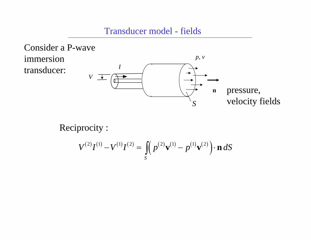
Reciprocity :( ) ( ) ( ) ( ) ( ) ( ) ( ) ( )( )2 1 1 2 2 1 1 2

S

V I V I p p dS− = − ⋅∫ v v n

Consider a P-waveimmersiontransducer:

pressure,velocity fields

p, v

VI

n

S

voltage

current

compressive force

velocity, v(x,ω)

( ) ( )( ) ( )

,

,S

v

F p dS

ω ω

ω ω

=

= ∫v x n

x

Transducer model- ‘lumped’ parameters

so reciprocity becomes:

( ) ( ) ( ) ( ) ( ) ( ) ( ) ( )2 1 1 2 2 1 1 2V I V I F v F v− = −

Forpiston behavior

( ) ( ) ( ) ( ), ,p dS F vω ω ω ω⋅ =∫ x v x n

VI

Fv

pressure, p(x,ω)

[TA]V

I

F

v

Transducer model - transfer matrix

VI

⎧ ⎨ ⎩

⎫ ⎬ ⎭

=T11

A T12A

T21A T22

A⎡

⎣ ⎢

⎤

⎦ ⎥

Fv

⎧ ⎨ ⎩

⎫ ⎬ ⎭

, det T A[ ]= 1

2-Port Transducer Model

From reciprocity

force

VI

F

v velocityA

I

[TA]V F

v

Transducer model - transfer matrix

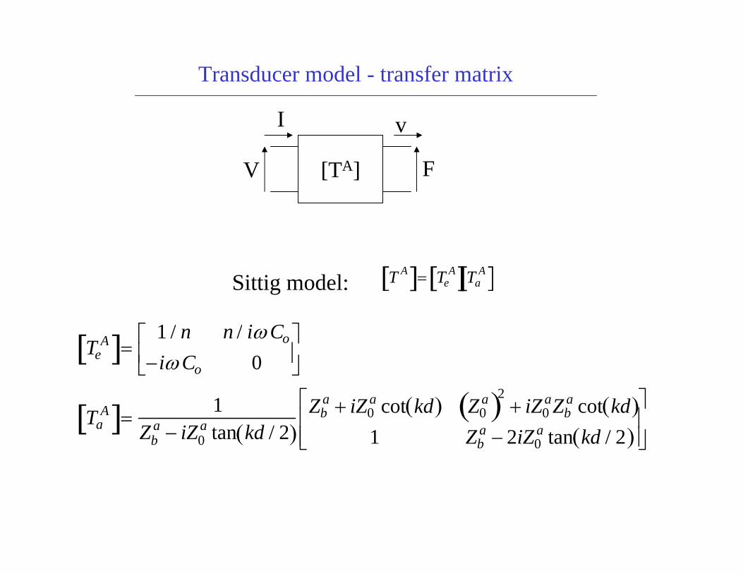
Sittig model: T A[ ]= TeA[ ]Ta

A[ ]

TeA[ ]=

1 / n n / iω Co

−iω Co 0⎡

⎣ ⎢ ⎤

⎦ ⎥

TaA[ ]= 1

Zba − iZ0

a tan kd / 2( )Zb

a + iZ0a cot kd( ) Z0

a( )2+ iZ0

aZba cot kd( )

1 Zba − 2iZ0

a tan kd / 2( )

⎡

⎣ ⎢ ⎢

⎤

⎦ ⎥ ⎥

Transducer model - transfer matrix

0

0 33

33

33 0

33

0

33

0 0

/

/

/,

Dp

D

p

Sss

D

ap

ab

k v

v c

c

n h Ch

C S dS d

Z v S

Z

ω

ρ

ρ

β

β

ρ

=

=

=

=

=

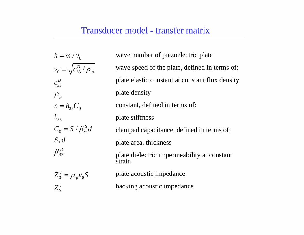
wave number of piezoelectric plate

wave speed of the plate, defined in terms of:

plate elastic constant at constant flux density

plate density

constant, defined in terms of:

plate stiffness

clamped capacitance, defined in terms of:

plate area, thickness

plate dielectric impermeability at constant strain

plate acoustic impedance

backing acoustic impedance

Transducer - three port model

IV

F2 , v2F1 , v1

transducer crystalPlating(thickness neglected)

F1

F2

V

⎧ ⎨ ⎪

⎩ ⎪

⎫ ⎬ ⎪

⎭ ⎪ = i

Z0a cot kl( ) Z0

a / sin kl( ) h33 / ωZ0

a / sin kl( ) Z0a cot kl( ) h33 / ω

h33 / ω h33 / ω 1/ ω C0

⎡

⎣

⎢ ⎢ ⎢

⎤

⎦

⎥ ⎥ ⎥

v1

v2

I

⎧ ⎨ ⎪

⎩ ⎪

⎫ ⎬ ⎪

⎭ ⎪

V I

F2

v2

F1

v1

3x3 impedance matrix

Transducer - Mason equivalent circuit

v1 v2

V

IF1F2

1: n

C0

- C0

iZ0 /sin(kl)a

- iZ0 tan(kl/2)a - iZ0 tan(kl/2)a

Transducer - KLM equivalent circuit model

1 : φ

- i X

C0V

I

F1

v1

F2

v2l/2 l/2

Z0Z0a a

φ =2M sin(kl/2)

1

X = Z0 M2 sin(kl)a

M = h33 / (ωZ0 )a

Sittig model with crystal facing layers

Backing (Zb )a

crystal facing layers(epoxy bonding, wear plate, etc.)

Acoustic layer: F1

v1

F2

v2

[Tl]

Commercial transducer:[TA] = [TA] [TA] [Tl] ...

F1

v1

⎧ ⎨ ⎩

⎫ ⎬ ⎭

=cos kala( ) −iZ0

a sin kala( )−isin kala( ) / Z0

a cos kala( )⎡

⎣ ⎢

⎤

⎦ ⎥

F2

v2

⎧ ⎨ ⎩

⎫ ⎬ ⎭

e a

[TA]V

I

Ft

v

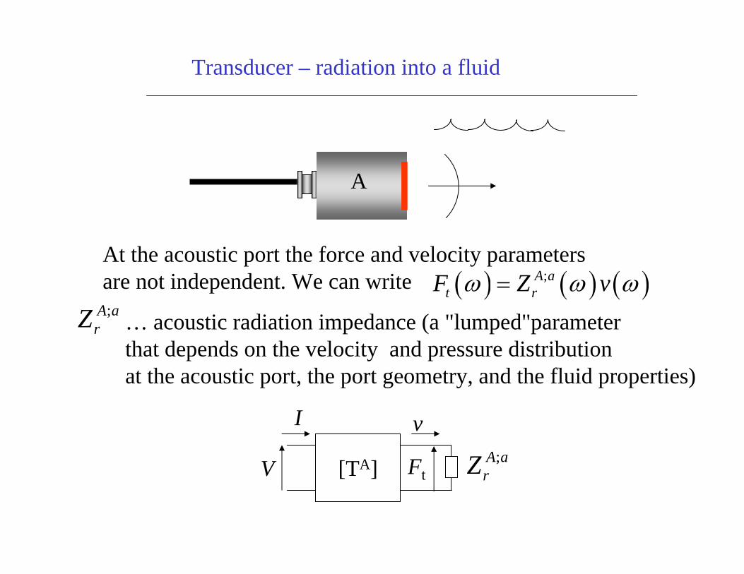
Transducer – radiation into a fluid

At the acoustic port the force and velocity parametersare not independent. We can write ( ) ( ) ( );A a

t rF Z vω ω ω=;A a

rZ … acoustic radiation impedance (a "lumped"parameter that depends on the velocity and pressure distributionat the acoustic port, the port geometry, and the fluid properties)

;A arZ

A

Acoustic radiation impedance

Rayleigh-Sommerfeld integral model of radiation ofwaves into a fluid by a piston transducer

( ) ( ) ( ) ( )exp,

2 S

i v ikrp dS

r

r

ω ρ ωω

π−

=

= −

∫x y

x y

( )( )

( )( ) ( ) ( )

,exp

2a sr

S S

p dSikriZ dS dS

v r

ωωρω

ω π⎧ ⎫−

= = ⎨ ⎬⎩ ⎭

∫∫ ∫

xy x

( )v ω

xyρ… fluid density

c … fluid wave speedk = ω/c

pressure

Greenspan, 1979: showed that for a circular piston transducer of radius a the acoustic radiation impedance obtained from the Rayleigh-Sommerfeld model could be found explicitly in the form

.

J1 … Bessel function

S1 … Struve function

SA = πa2

Acoustic radiation impedance

( ) ( );1 1/ 1 /A a

r AZ cS J ka iS ka kaρ = − −⎡ ⎤⎣ ⎦

Acoustic radiation impedance

>> ka=linspace(0, 25, 100);

>> ka = ka + eps*( ka ==0);

>> Z = 1 -(besselj(1,ka)-i*struve(ka))./ka;

>> plot(ka, abs(Z))

>> xlabel(' ka ')

>> ylabel( ' V/\rhocS')

>> ylabel( ' Z/\rhocS')

0 5 10 15 20 250.5

0.6

0.7

0.8

0.9

1

1.1

1.2

;A ar

A

ZcSρ

ka

Greenspan model of a circular piston transducer

velocity

Fv

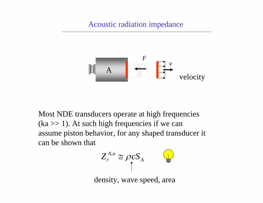
Acoustic radiation impedance

Most NDE transducers operate at high frequencies (ka >> 1). At such high frequencies if we canassume piston behavior, for any shaped transducer it can be shown that

;A ar AZ cSρ≅

density, wave speed, area

A

function y = struve(z)num = length(z);y=zeros(1,num);for k = 1:numy(k) = quadl(@struve_arg, 0, 1, [ ],[ ], z(k));end

function y = struve_arg(x, z)

y = (4./pi).*z.*x.^2.*sin(z.*(1-x.^2)).*sqrt(2-x.^2);

Acoustic radiation impedance

( ) ( )

( )

12 2

10

12 2 2

0

2 1 sin 1

4 sin 1 2

zH z t zt dt t x

z x z x x dx

π

π

= − = −

⎡ ⎤= − −⎣ ⎦

∫

∫

this uses

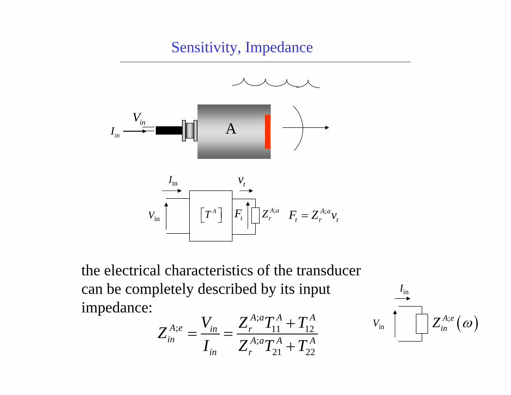
Sensitivity, Impedance

Vin

Iin

;A arZAT⎡ ⎤⎣ ⎦ tF

tv

;A at r tF Z v=

;; 11 12

;21 22

A a A AA e in rin A a A A

in r

V Z T TZI Z T T

+= =

+

inVinI

the electrical characteristics of the transducercan be completely described by its inputimpedance:

Iin

Vin ( );A einZ ω

A

Sensitivity, Impedance

inVinI

The particular sensitivity we will use is:

;21 22

1A tvI A a A A

in r

vSI Z T T

≡ =+

to describe the conversion of electrical signals into acoustic signals, we could use the transducer's sensitivity, SOI, where

tv

tF

OIOSI

=

O … an output (force or velocity)I … an input (voltage or current)

A

Sensitivity, Impedance

;A at r tF Z v=

All the other sensitivities can be found from this sensitivity if the transducer electrical impedance and acoustic radiation impedance are known:

;

;

; ;

/

/

A tvI

in

A A a AtFI r vI

in

A A A etvV vI in

in

A A a A A etFV r vI in

in

vSIFS Z SIvS S ZVFS Z S ZV

=

= =

= =

= =

inVinI

tF

tvA

;A einZ

inI

inV

At vI inv S I=

inVinI

tv

tFA

Sensitivity, Impedance

Thus, we can replace the transfer matrix model of the transducerby a model consisting of an electrical impedance and an ideal "converter" that is defined by the transducer sensitivity:

;A a At r vI inF Z S I=

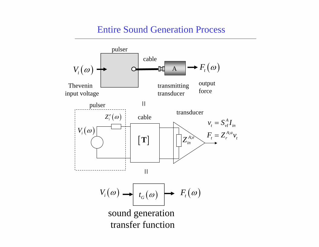
Entire Sound Generation Process

( )tF ω

transmittingtransducer

cablepulser

( )iV ωoutputforce

( )iV ω ( )tF ω( )Gt ω

Thevenininput voltage

A

( )iV ω

( )eiZ ω

[ ]T ;A einZ

;

At vI in

A at r t

v S I

F Z v

=

=

pulser

cabletransducer

sound generationtransfer function

==

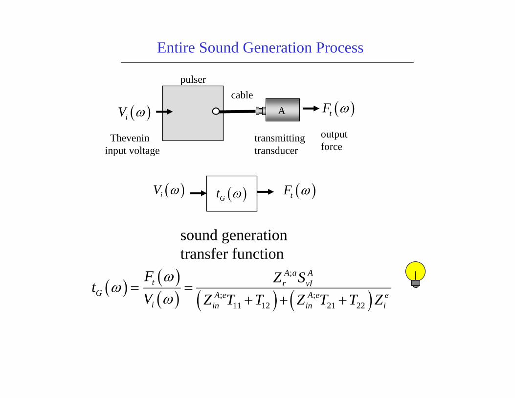
Entire Sound Generation Process

( )tF ω

transmittingtransducer

cablepulser

( )iV ωoutputforce

Thevenininput voltage

A

( )iV ω ( )tF ω( )Gt ω

( ) ( )( ) ( ) ( )

;

; ;11 12 21 22

A a At r vI

G A e A e ei in in i

F Z StV Z T T Z T T Z

ωω

ω= =

+ + +

sound generationtransfer function

References

Ristic, V.M., Principles of Acoustic Devices, John Wiley, 1983

Kino. G.S., Acoustic Waves - Devices, Imaging and Analog Signal Processing, Prentice-Hall, 1987.

Auld, B.A., Acoustic Fields and Waves in Solids, 2nd Ed., Vols. I and II, Krieger Publishing Co. , 1990.

Sacshe, W., and N.N. Hsu,” Ultrasonic transducers for materials testing and their characterization,” in Physical Acoustics, Vol. XIV,Eds. W.P. Mason and R.N. Thurston, 277-406, 1979.

Greeenspan, M., “Piston radiator: some extension of the theory,”J. Acoust. Soc. Am., 65, 608-621, 1979.