transfer function models of dynamical processes · process control time domain transfer function...
TRANSCRIPT
1
Transfer Function Modelsof Dynamical Processes
Process Dynamics and ControlProcess Dynamics and Control

2
Linear SISOLinear SISO Control SystemsControl Systems
General form of a linear SISO control system:General form of a linear SISO control system:
this is a underdeterminedthis is a underdetermined higher order differentialhigher order differentialequationequation
thethe functionfunction must be specified for this ODE tomust be specified for this ODE toadmit a well defined solutionadmit a well defined solution

3
Transfer FunctionTransfer Function
Heated stirred-tank model (constant flow, )Heated stirred-tank model (constant flow, )
Taking the Taking the Laplace Laplace transform yields:transform yields:
or lettingor letting
Transfer functions

4
Transfer FunctionTransfer Function
Heated stirred tank exampleHeated stirred tank example
e.g. e.g. The block is called the transfer function relating Q(s) to T(s)
+
++
5
Process ControlProcess Control
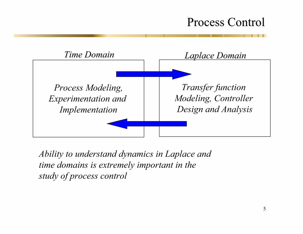
Time DomainTime Domain
Transfer function Modeling, Controller Design and Analysis
Process Modeling,Experimentation and
Implementation
Laplace Laplace DomainDomain
Ability to understand dynamics in Laplace and time domains is extremely important in thestudy of process control

6
Transfer functionsTransfer functions
Transfer functions are generallyTransfer functions are generally expressed as a ratio ofexpressed as a ratio ofpolynomialspolynomials
WhereWhere
The polynomial is called the The polynomial is called the characteristic polynomialcharacteristic polynomial of of
Roots ofRoots of are theare the zeroeszeroes of of Roots ofRoots of are the are the polespoles of of

7
Transfer functionTransfer function
Order of underlying ODE is given by degree ofcharacteristic polynomial
e.g. First order processes
Second order processes
Order of the process is the degree of the characteristic(denominator) polynomial
The relative order is the difference between the degree of thedenominator polynomial and the degree of the numeratorpolynomial
8
Transfer FunctionTransfer Function
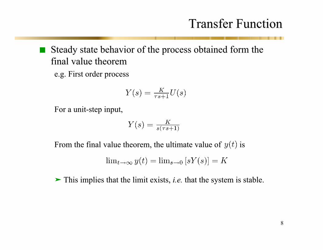
Steady state behavior of the process obtained form theSteady state behavior of the process obtained form thefinal value theoremfinal value theoreme.g. First ordere.g. First order processprocess
For a unit-step input,For a unit-step input,
From the finalFrom the final value theorem, the ultimate value ofvalue theorem, the ultimate value of isis
This implies that the limit exists,This implies that the limit exists, i.e.i.e. that the system is that the system is stable.stable.
9
Transfer functionTransfer function
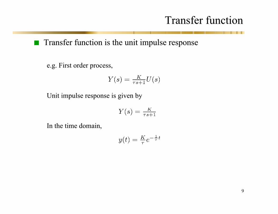
Transfer function is the unit impulse responseTransfer function is the unit impulse response
e.g.e.g. First order process,First order process,
Unit impulse responseUnit impulse response is given byis given by
In the time domain,In the time domain,

10
Transfer FunctionTransfer Function
Unit impulse response of a 1st order processUnit impulse response of a 1st order process
11
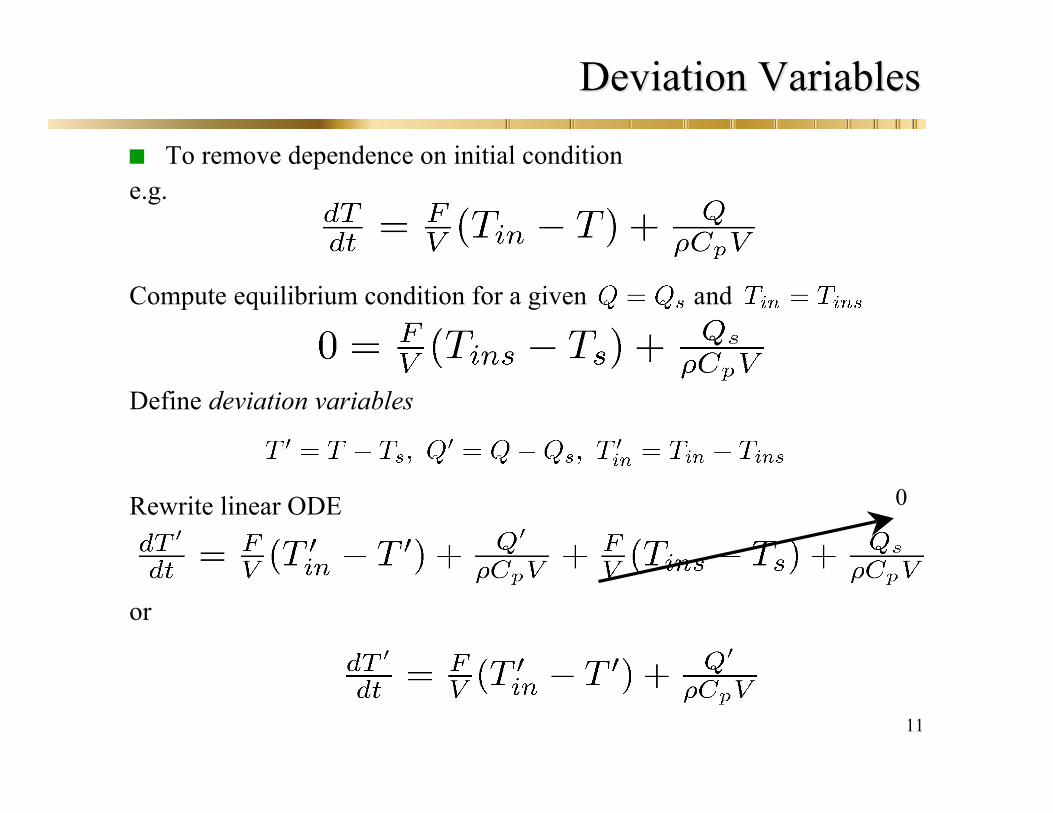
Deviation VariablesDeviation Variables
To remove dependence on initial conditione.g.
Compute equilibrium condition for a given and
Define deviation variables
Rewrite linear ODE
or
0
12
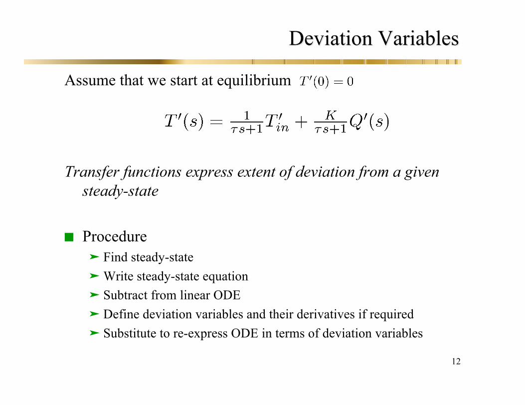
Deviation VariablesDeviation Variables
Assume that we start at equilibrium
Transfer functions express extent of deviation from a givensteady-state
Procedure Find steady-stateWrite steady-state equation Subtract from linear ODEDefine deviation variables and their derivatives if required Substitute to re-express ODE in terms of deviation variables

13
Process ModelingProcess Modeling
Gravity tank
Objectives:Objectives: height of liquid in tankFundamental quantity:Fundamental quantity: Mass, momentumAssumptions:Assumptions:
Outlet flow is driven by head of liquid in the tank Incompressible flow Plug flow in outlet pipe Turbulent flow
h
L
F
Fo

14
Transfer FunctionsTransfer Functions
From mass balance and Newton’s law,
A system of simultaneous ordinary differential equations results
Linear or nonlinear?
15
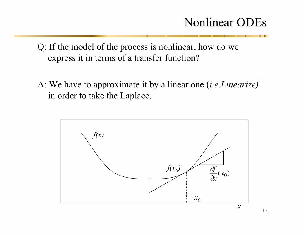
Nonlinear Nonlinear ODEsODEs
Q: If the model of the process is nonlinear, how do weexpress it in terms of a transfer function?
A: We have to approximate it by a linear one (i.e.Linearize)in order to take the Laplace.
f(x0)
f(x)
!!fxx( )0
xx0

16
Nonlinear systemsNonlinear systems
First order Taylor series expansion
1. Function of one variable
2. Function of two variables
3. ODEs

17
Transfer Transfer FFunctionunction
Procedure to obtain transfer function from nonlinearprocess models Find an equilibrium point of the system Linearize about the steady-state Express in terms of deviations variables about the steady-state Take Laplace transform Isolate outputs in Laplace domain
Express effect of inputs in terms of transfer functions

18
Block DiagramsBlock Diagrams
Transfer functions of complex systems can be representedTransfer functions of complex systems can be representedin block diagram form.in block diagram form.
3 basic arrangements of transfer functions:3 basic arrangements of transfer functions:
1.1. Transfer functions in seriesTransfer functions in series
2.2. Transfer functions in parallelTransfer functions in parallel
3.3. Transfer functions in feedback formTransfer functions in feedback form

19
Block DiagramsBlock Diagrams
Transfer functions in seriesTransfer functions in series
Overall operation is the multiplication of transfer functionsOverall operation is the multiplication of transfer functions
Resulting overall transfer functionResulting overall transfer function

20
Block DiagramsBlock Diagrams
Transfer functions in series (two first order systems)Transfer functions in series (two first order systems)
Overall operation is the multiplication of transfer functionsOverall operation is the multiplication of transfer functions
Resulting overall transfer functionResulting overall transfer function

21
Transfer FunctionsTransfer Functions
DCDC Motor example:Motor example: In terms of angular velocityIn terms of angular velocity
In terms of the angleIn terms of the angle
22
Transfer FunctionsTransfer Functions
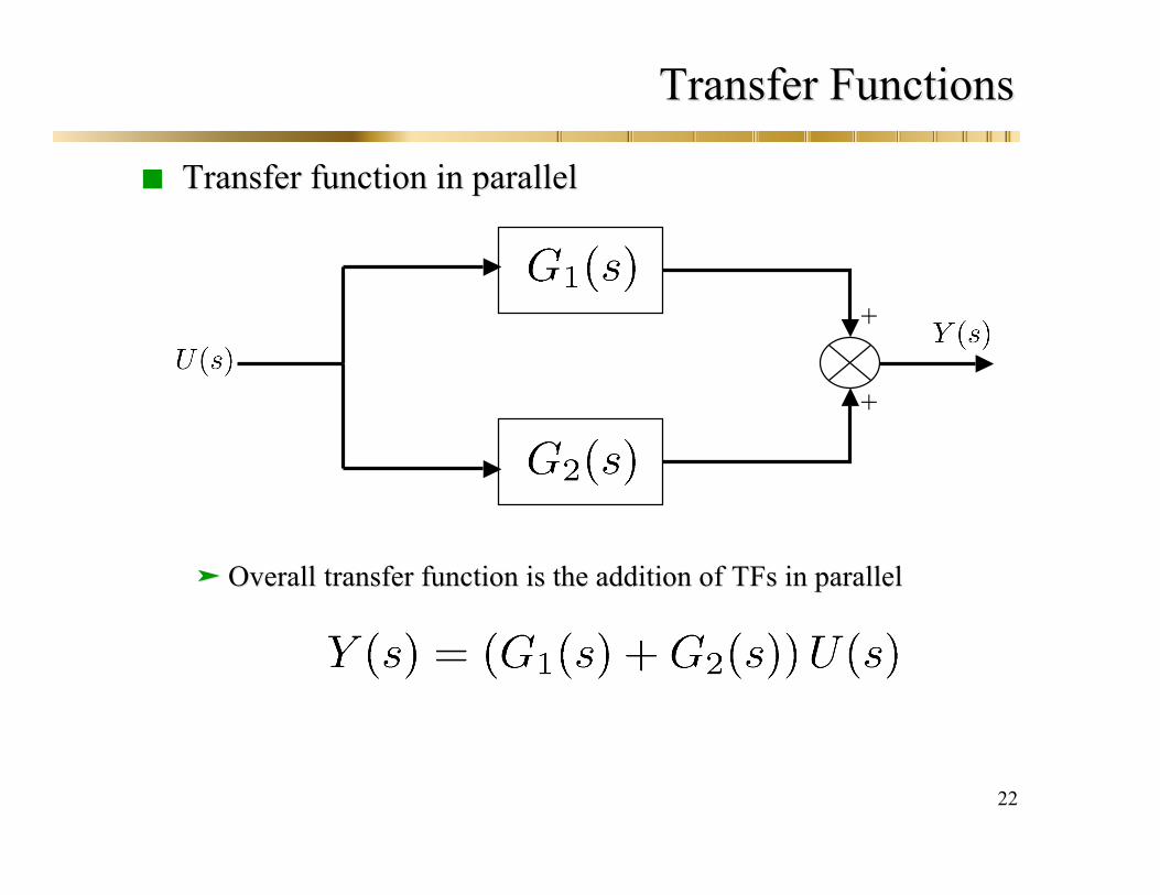
Transfer function in parallelTransfer function in parallel
OverallOverall transfer function is the addition oftransfer function is the addition of TFs TFs in parallelin parallel
+
+

23
Transfer FunctionsTransfer Functions
Transfer function in parallelTransfer function in parallel
OverallOverall transfer function is the addition oftransfer function is the addition of TFs TFs in parallelin parallel
+
+
24
Transfer FunctionsTransfer Functions
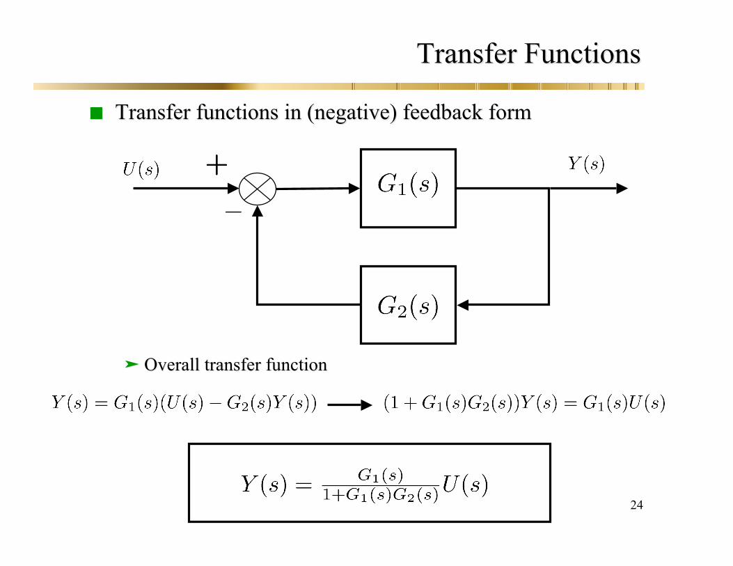
Transfer functions in (negative) feedback formTransfer functions in (negative) feedback form
Overall transfer functionOverall transfer function

25
Transfer FunctionsTransfer Functions
Transfer functions in (positive) feedback formTransfer functions in (positive) feedback form
Overall transfer functionOverall transfer function

26
Transfer FunctionTransfer Function
Example 3.20Example 3.20
27
Transfer FunctionTransfer Function
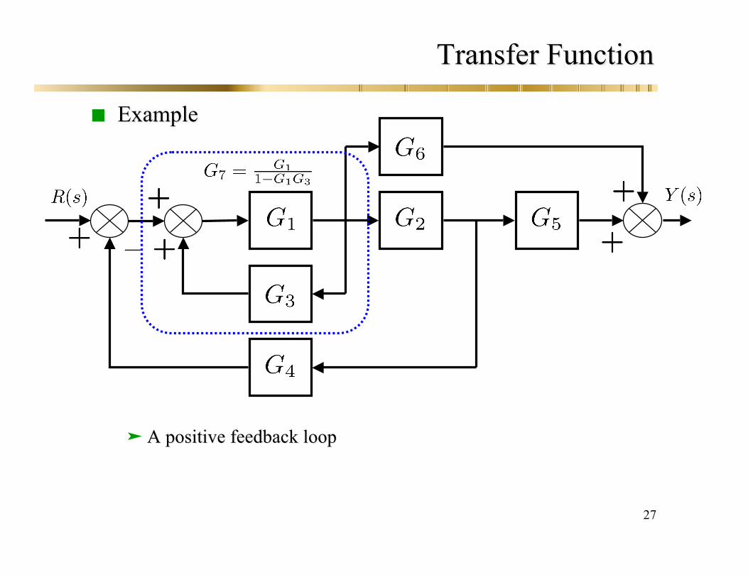
ExampleExample
A positive feedback loopA positive feedback loop

28
Transfer FunctionTransfer Function
Example 3.20Example 3.20
Two systems in parallelTwo systems in parallel ReplaceReplace byby

29
Transfer FunctionTransfer Function
Example 3.20Example 3.20
Two systems in parallelTwo systems in parallel

30
Transfer FunctionTransfer Function
Example 3.20Example 3.20
A negative feedback loopA negative feedback loop

31
Transfer FunctionTransfer Function
Example 3.20Example 3.20
Two process in seriesTwo process in series
32
First Order SystemsFirst Order Systems
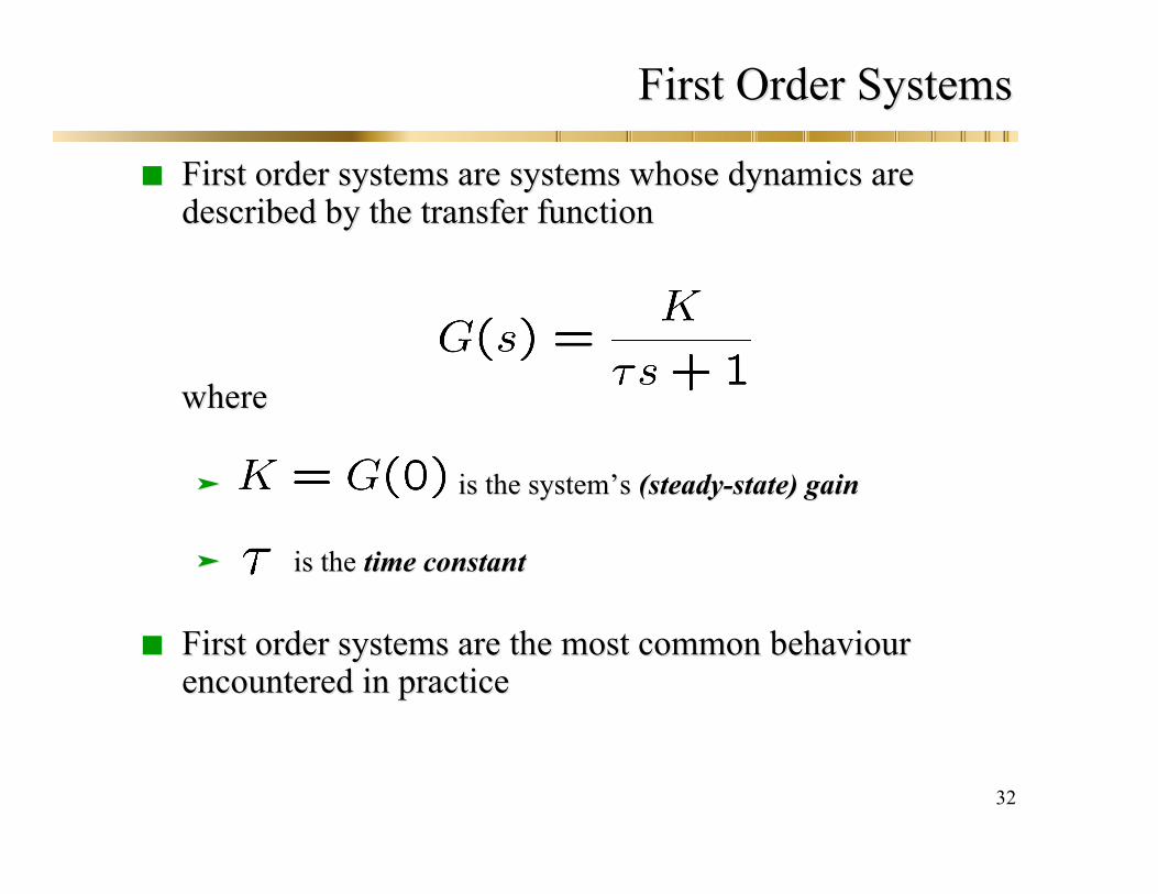
First order systemsFirst order systems are systems whose dynamics areare systems whose dynamics aredescribed by the transfer functiondescribed by the transfer function
wherewhere
is the systemis the system’’s s (steady-state) gain(steady-state) gain
is the is the time constanttime constant
First orderFirst order systems are the most common systems are the most common behaviourbehaviourencountered in practiceencountered in practice

33
First Order SystemsFirst Order Systems
ExamplesExamples, Liquid storage
Assume: Incompressible flow Outlet flow due to gravity
Balance equation: Total Flow In Flow Out
34
First Order SystemsFirst Order Systems
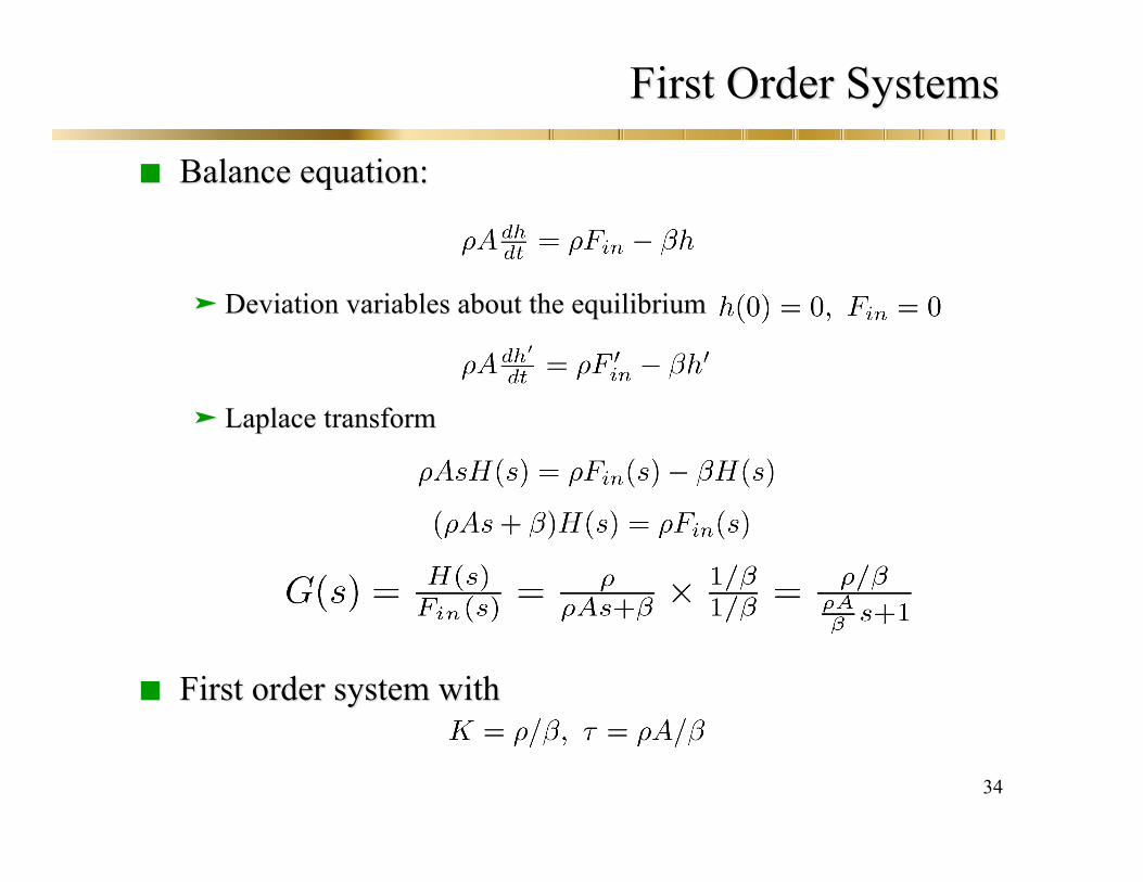
Balance equation:Balance equation:
Deviation variables about the equilibriumDeviation variables about the equilibrium
Laplace Laplace transformtransform
First order system withFirst order system with
35
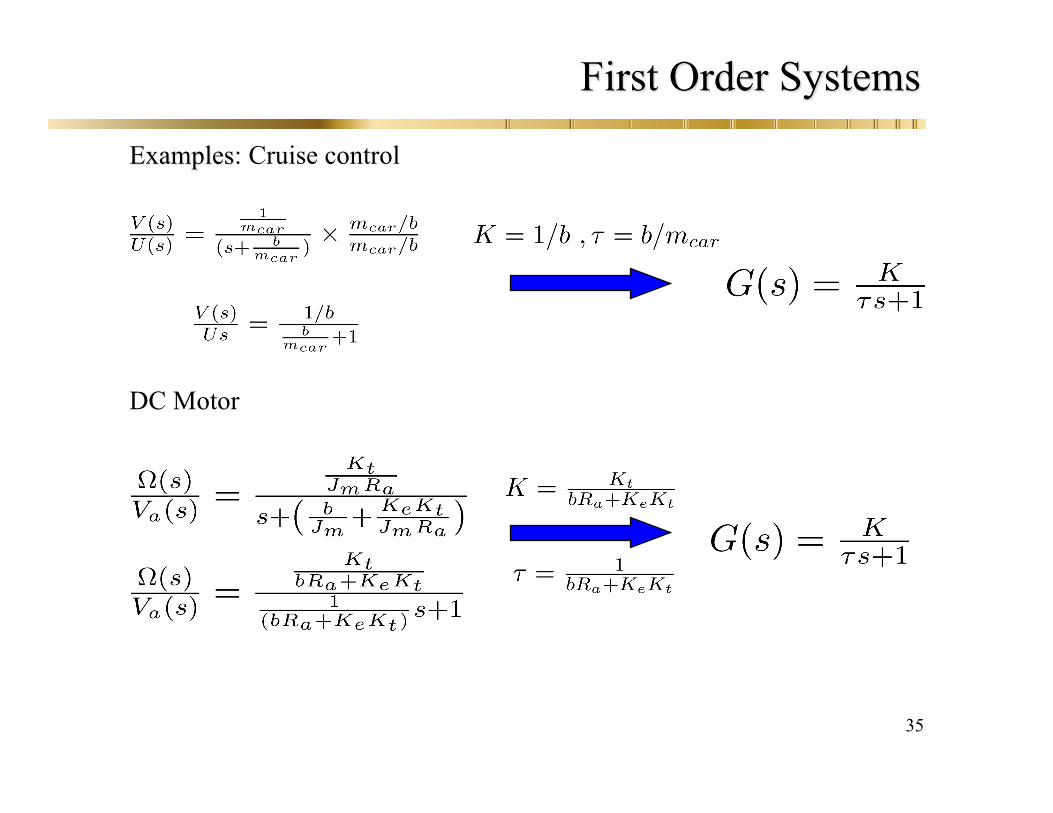
First Order SystemsFirst Order Systems
ExamplesExamples: Cruise control
DC Motor
36
First Order SystemsFirst Order Systems
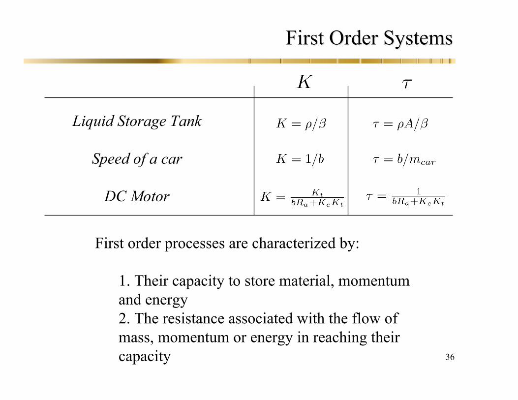
Liquid Storage Tank
Speed of a car
DC Motor
First order processes are characterized by:
1. Their capacity to store material, momentum and energy2. The resistance associated with the flow of mass, momentum or energy in reaching theircapacity
37
First Order SystemsFirst Order Systems
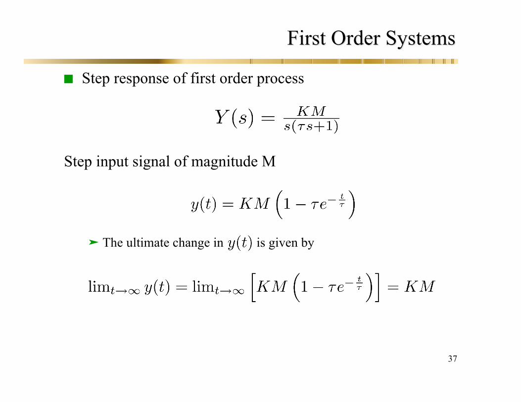
Step response of first order process
Step input signal of magnitude M
The ultimate change in is given by
38
First Order SystemsFirst Order Systems
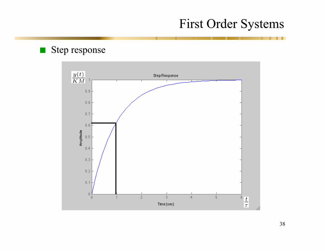
Step responseStep response

39
First Order SystemsFirst Order Systems
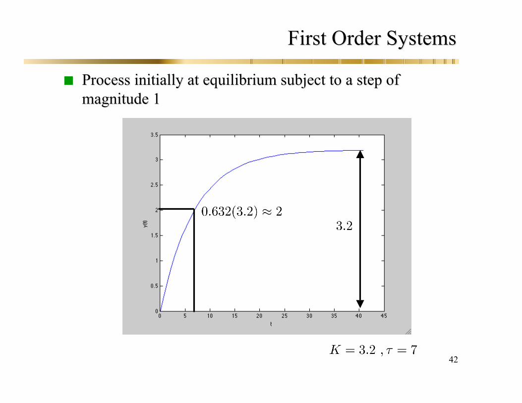
What do we look for?What do we look for? SystemSystem’’s Gain: Steady-State Responses Gain: Steady-State Response
Process Time Constant:Process Time Constant:
What do we need?What do we need? System initially atSystem initially at equilibriumequilibrium Step input of magnitude MStep input of magnitude M Measure process gain from new steady-stateMeasure process gain from new steady-state Measure time constantMeasure time constant
Time Required to Reach 63.2% of final value

40
First Order SystemsFirst Order Systems
First order systems areFirst order systems are also called systems with finitealso called systems with finitesettling timesettling time The settling time is the time required for the system comesThe settling time is the time required for the system comes
within 5% of the total change and stays 5%within 5% of the total change and stays 5% for all timesfor all times
Consider the step responseConsider the step response
The overall change isThe overall change is

41
First Order SystemsFirst Order Systems
Settling timeSettling time
42
First Order SystemsFirst Order Systems
Process initially at equilibrium subject to a step ofProcess initially at equilibrium subject to a step ofmagnitude 1magnitude 1

43
First order processFirst order process
Ramp response:Ramp response:
Ramp input of slope a
0 0.5 1 1.5 2 2.5 3 3.5 4 4.5 50
0.5
1
1.5
2
2.5
3
3.5
4
4.5
5
44
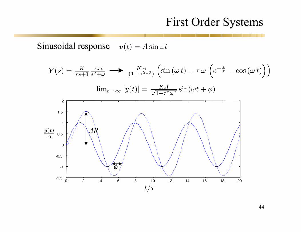
First OrderFirst Order SystemsSystems
Sinusoidal responseSinusoidal response
Sinusoidal input Asin(ωt)
0 2 4 6 8 10 12 14 16 18 20-1.5
-1
-0.5
0
0.5
1
1.5
2
AR
φ

45
First Order SystemsFirst Order Systems
10 -2 10 -1 10 0 10 1 10 210 -2
10 -1
10 0Bode Plots
10 -2 10 -1 10 0 10 1 10 2-100
-80-60
-40-20
0
High Frequency
AsymptoteCorner Frequency
Amplitude Ratio Phase Shift

46
Integrating SystemsIntegrating Systems
Example: Liquid storage tankExample: Liquid storage tank
Laplace Laplace domaindomain dynamicsdynamics
If there is no outlet flow,If there is no outlet flow,
h
F
Fi
47
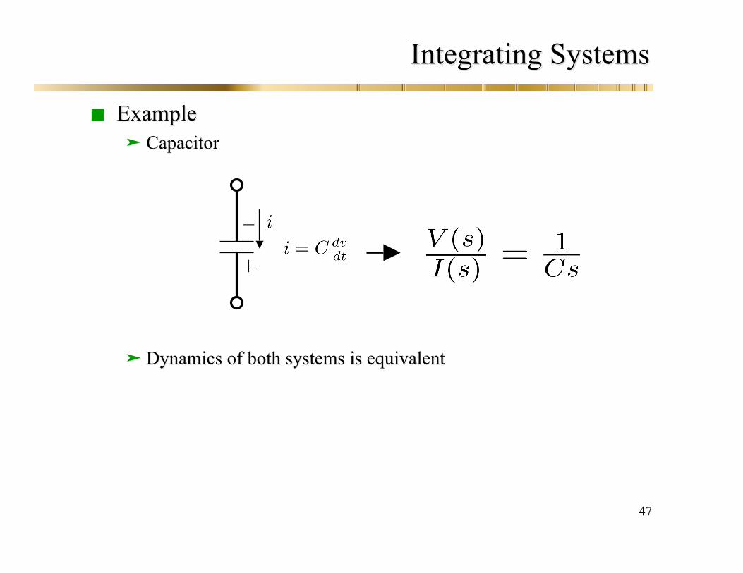
Integrating SystemsIntegrating Systems
ExampleExample CapacitorCapacitor
Dynamics of both systems is equivalentDynamics of both systems is equivalent

48
Integrating SystemsIntegrating Systems
Step input of magnitude MStep input of magnitude M
Out
put
Time
Inpu
t
Time
Slope =

49
Integrating SystemsIntegrating Systems
Unit impulse responseUnit impulse response
Out
put
Time
Inpu
t
Time
50
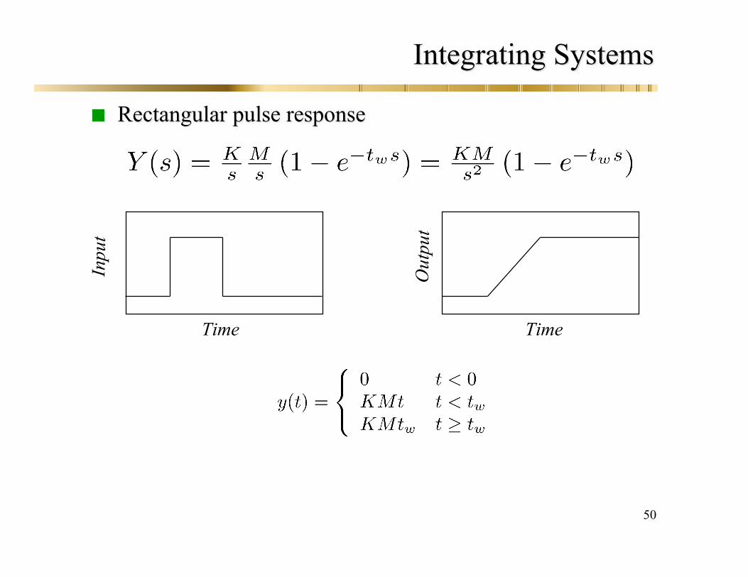
Integrating SystemsIntegrating Systems
Rectangular pulse responseRectangular pulse response
Out
put
Time
Inpu
t
Time

51
Second order SystemsSecond order Systems
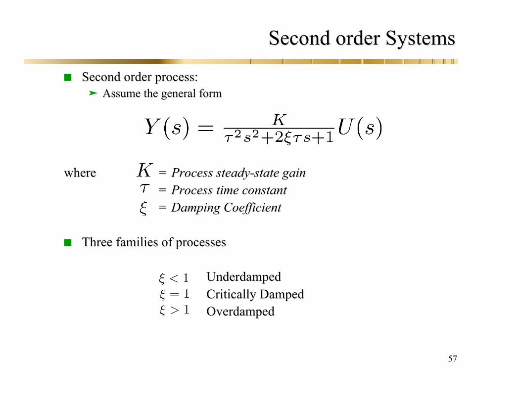
Second order process:Second order process: Assume the general formAssume the general form
wherewhere = Process steady-state gain= Process steady-state gain= Process time constant= Process time constant= Damping Coefficient= Damping Coefficient
Three families of processesThree families of processes
UnderdampedUnderdampedCritically DampedCritically DampedOverdampedOverdamped

52
Second Order SystemsSecond Order Systems
Three types of second order process:
1. Two First Order Systems in series or in parallele.g. Two holding tanks in series
2. Inherently second order processes: Mechanical systemspossessing inertia and subjected to some external forcee.g. A pneumatic valve
3. Processing system with a controller: Presence of acontroller induces oscillatory behaviore.g. Feedback control system

53
Second order SystemsSecond order Systems
Multicapacity Multicapacity Second Order ProcessesSecond Order Processes Naturally arise from two first order processes in seriesNaturally arise from two first order processes in series
By multiplicative property of transfer functionsBy multiplicative property of transfer functions

54
Transfer FunctionsTransfer Functions
First order systems in parallelFirst order systems in parallel
OverallOverall transfer function a second order process (with one zero)transfer function a second order process (with one zero)
+
+

55
Second Order SystemsSecond Order Systems
Inherently second order process:Inherently second order process:e.g. Pneumatic Valve
x
p
By Newton’s law
56
Second Order SystemsSecond Order Systems
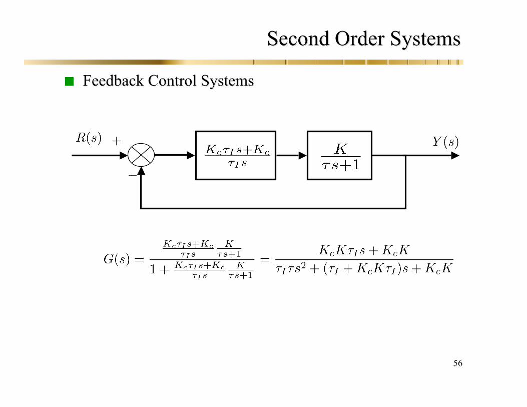
Feedback Control SystemsFeedback Control Systems
57
Second order SystemsSecond order Systems
Second order process:Second order process: Assume the general formAssume the general form
wherewhere = Process steady-state gain= Process steady-state gain= Process time constant= Process time constant= Damping Coefficient= Damping Coefficient
Three families of processesThree families of processes
UnderdampedUnderdampedCritically DampedCritically DampedOverdampedOverdamped
58
Second Order SystemsSecond Order Systems
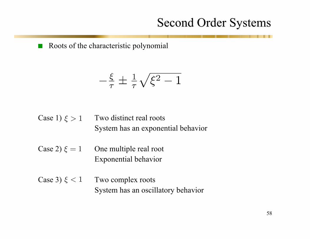
Roots of the characteristic polynomial
Case 1) Two distinct real rootsSystem has an exponential behavior
Case 2) One multiple real rootExponential behavior
Case 3) Two complex rootsSystem has an oscillatory behavior

59
Second Order SystemsSecond Order Systems
Step response of magnitude MStep response of magnitude M
0 1 2 3 4 5 6 7 8 9 100
0.2
0.4
0.6
0.8
1
1.2
1.4
1.6
1.8
2
ξ=2
ξ=0
ξ=0.2

60
Second Order SystemsSecond Order Systems
Observations
Responses exhibit overshoot when
Large yield a slow sluggish response
Systems with yield the fastest response without overshoot
As (with ) becomes smaller, system becomes moreoscillatory

61
Second Order SystemsSecond Order Systems
Characteristics of underdamped second order process
1. Rise time,2. Time to first peak,3. Settling time,4. Overshoot:
5. Decay ratio:

62
Second Order SystemsSecond Order Systems
Step responseStep response

63
Second Order SystemsSecond Order Systems
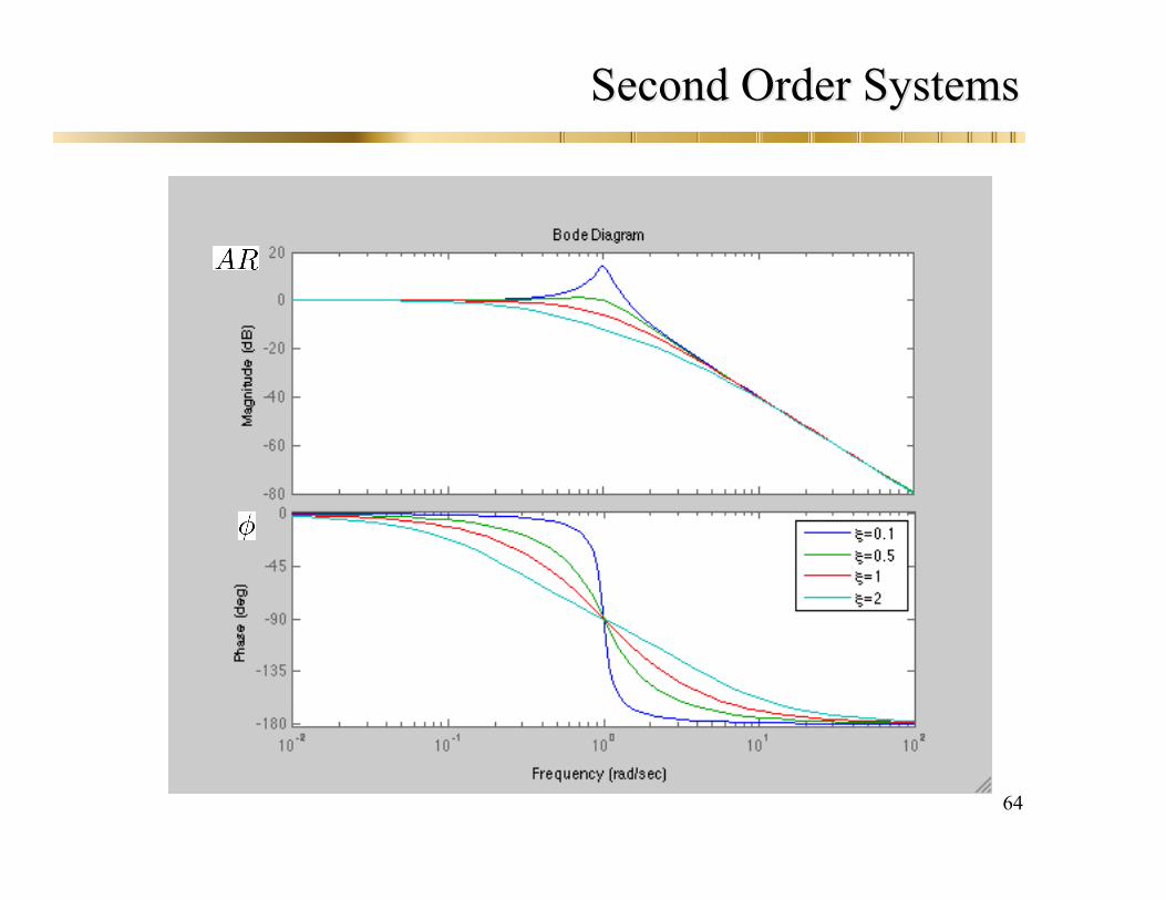
Sinusoidal ResponseSinusoidal Response
wherewhere
64
Second Order SystemsSecond Order Systems
65
More Complicated SystemsMore Complicated Systems
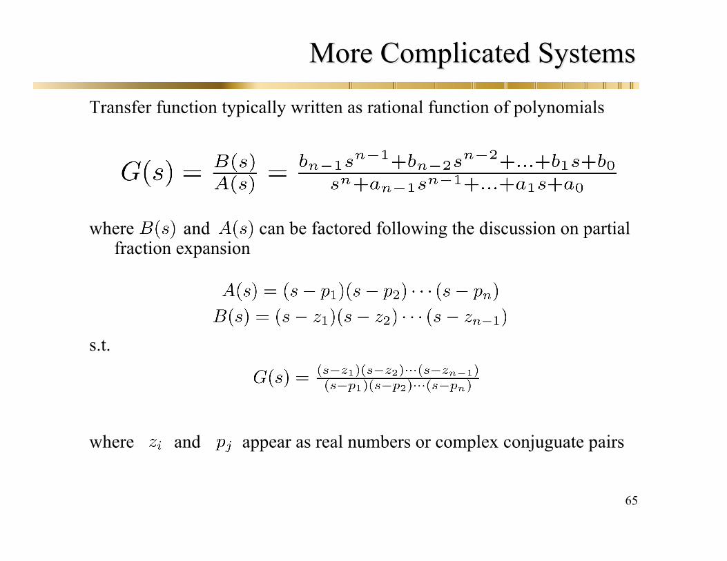
Transfer function typically written as rational function of polynomials
where and can be factored following the discussion on partialfraction expansion
s.t.
where and appear as real numbers or complex conjuguate pairs

66
Poles and zeroesPoles and zeroes
Definitions: the roots of are called the zeroszeros of G(s)
the roots of are called the polespoles of G(s)
Poles: Directly related to the underlying differential equation
If , then there are terms of the form in vanishes to a unique point
If any then there is at least one term of the form does not vanish

67
PolesPoles
e.g. A transfer function of the form
with can factored to a sum of
A constant term from A from the term A function that includes terms of the form
Poles can help us to describe the qualitative behavior of a complex system(degree>2)
The sign of the poles gives an idea of the stability of the system

68
Poles
Calculation performed easily in MATLAB Function POLE, PZMAP
e.g.» s=tf(‘s’);» sys=1/s/(s+1)/(4*s^2+2*s+1);Transfer function:Transfer function: 1 1--------------------------------------------------4 s^4 + 6 s^3 + 3 s^2 + s4 s^4 + 6 s^3 + 3 s^2 + s» pole(sys)ans ans == 0 0 -1.0000 -1.0000 -0.2500 + 0.4330i -0.2500 + 0.4330i -0.2500 - 0.4330i -0.2500 - 0.4330i MATLAB

69
PolesPoles
Function PZMAPFunction PZMAP» pzmap(sys) MATLAB
70
PolesPoles
One constant poleOne constant pole integrating featureintegrating feature
One real negative poleOne real negative pole decaying exponentialdecaying exponential
A pair of complex roots with negative real partA pair of complex roots with negative real part decaying sinusoidaldecaying sinusoidal
What is the dominant feature?What is the dominant feature?
71
PolesPoles
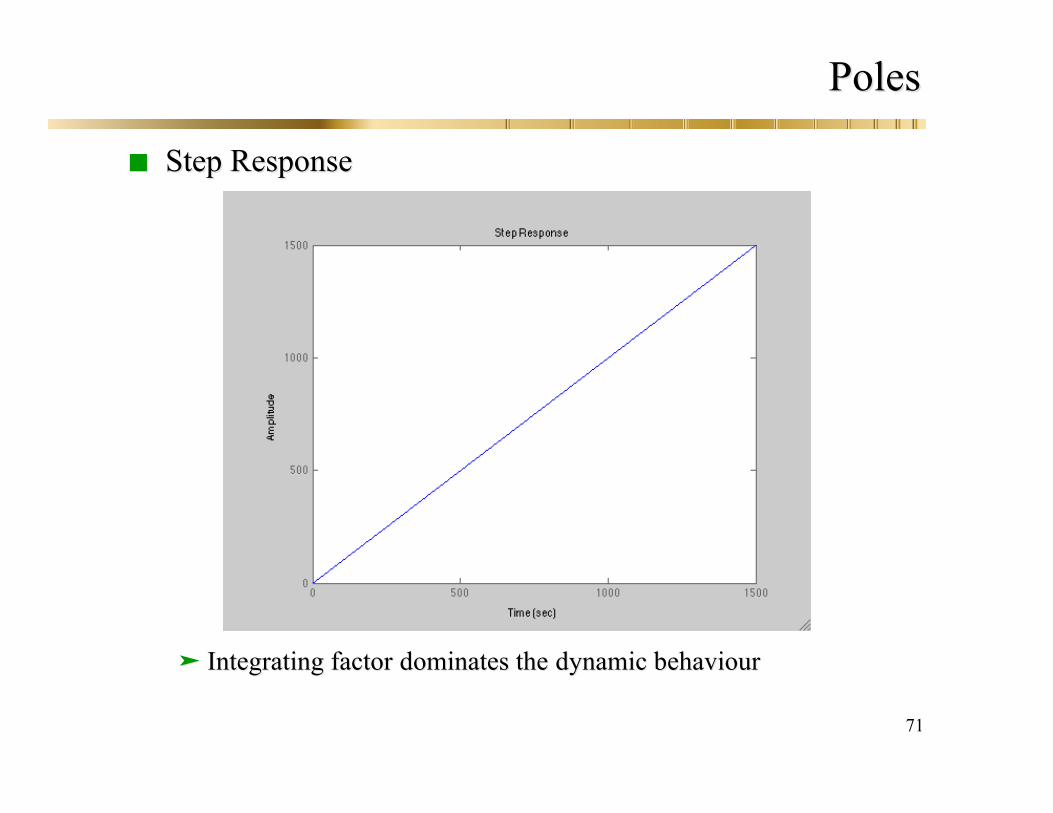
Step ResponseStep Response
Integrating factorIntegrating factor dominates thedominates the dynamic dynamic behaviourbehaviour

72
PolesPoles
ExampleExample
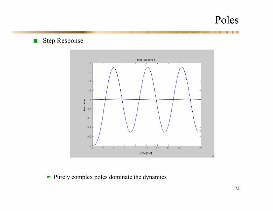
PolesPoles -1.0000-1.0000
-0.0000 + 1.0000i-0.0000 + 1.0000i -0.0000 - 1.0000i-0.0000 - 1.0000i
One negative real poleOne negative real pole Two purely complex polesTwo purely complex poles
What is the dominant feature?What is the dominant feature?
73
PolesPoles
Step ResponseStep Response
Purely complex poles dominate the dynamicsPurely complex poles dominate the dynamics
74
PolesPoles
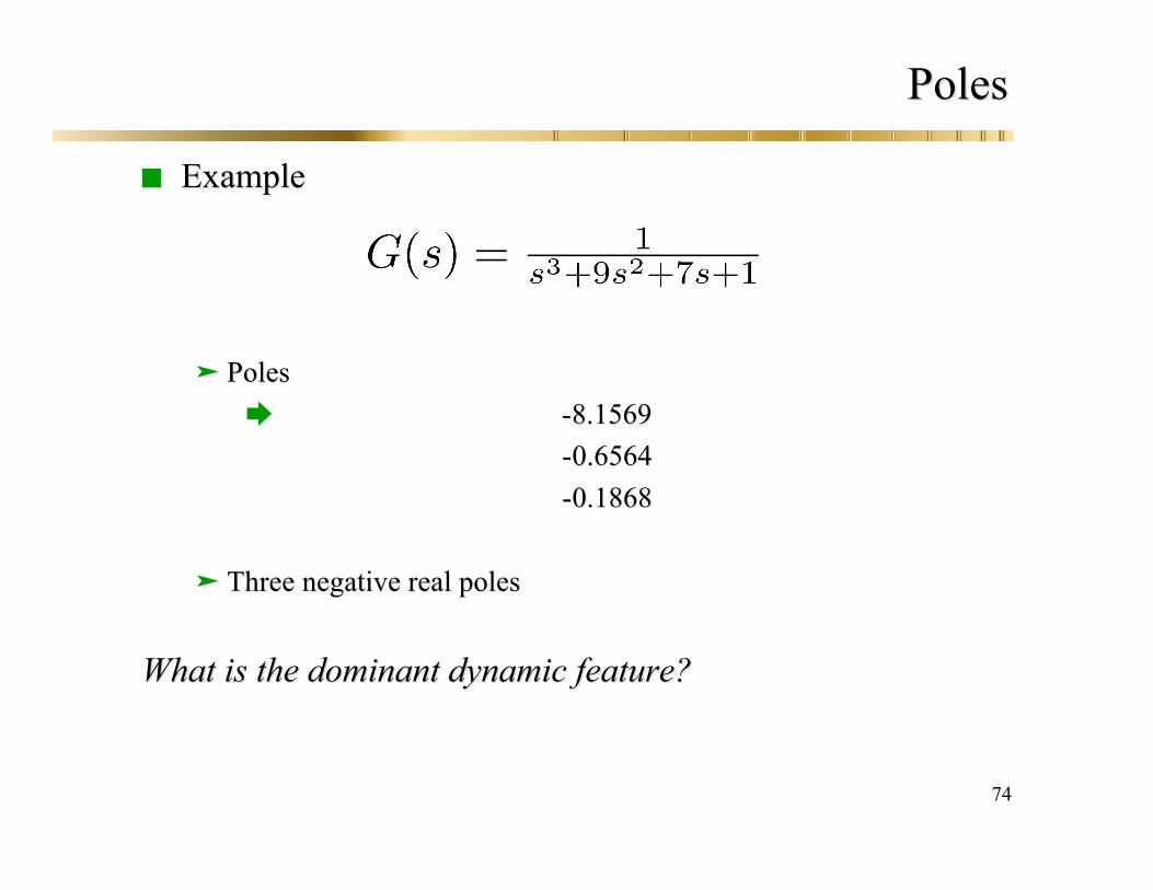
ExampleExample
PolesPoles -8.1569-8.1569
-0.6564-0.6564 -0.1868-0.1868
Three negative real polesThree negative real poles
What is the dominant dynamic feature?What is the dominant dynamic feature?

75
PolesPoles
Step ResponseStep Response
Slowest exponential (Slowest exponential ( ) dominates the dynamic) dominates the dynamicfeature (yields a time constant of 1/0.1868= 5.35 sfeature (yields a time constant of 1/0.1868= 5.35 s
76
PolesPoles
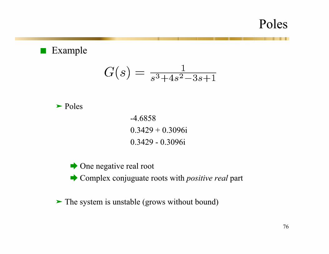
ExampleExample
PolesPoles -4.6858-4.6858 0.3429 + 0.3096i0.3429 + 0.3096i 0.3429 - 0.3096i0.3429 - 0.3096i
One negative real rootOne negative real root Complex Complex conjuguate conjuguate roots withroots with positive realpositive real part part
The system is unstable (grows without bound)The system is unstable (grows without bound)

77
PolesPoles
Step ResponseStep Response

78
PolesPoles
Two types of polesTwo types of poles
Slow (or dominant) polesSlow (or dominant) poles Poles that are closer toPoles that are closer to the imaginary axisthe imaginary axis
Smaller real part means Smaller real part means smaller exponential termsmaller exponential term andandslower decayslower decay
Fast polesFast poles Poles that are further from thePoles that are further from the imaginary axisimaginary axis
LargerLarger real part means larger exponentialreal part means larger exponential term and fasterterm and fasterdecaydecay

79
PolesPoles
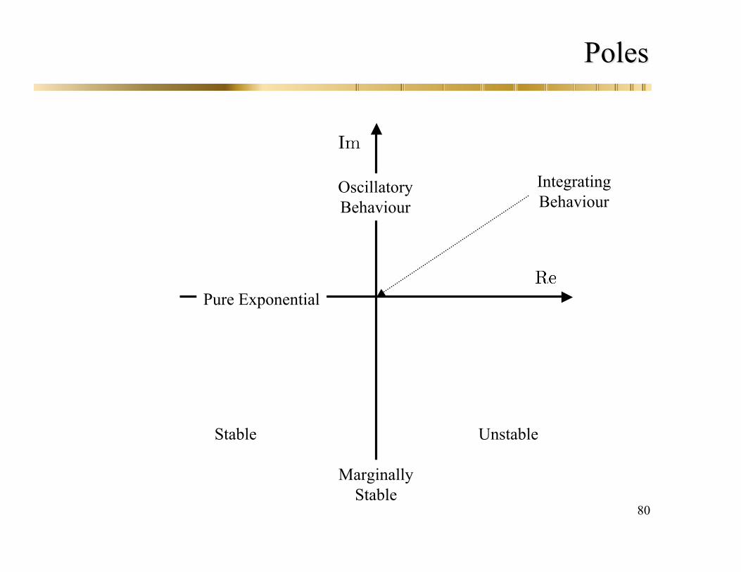
PolesPoles dictate the stability of the processdictate the stability of the process
Stable polesStable poles Poles with negative real partsPoles with negative real parts Decaying exponentialDecaying exponential
Unstable polesUnstable poles Poles withPoles with positive real partspositive real parts Increasing exponentialIncreasing exponential
Marginally stable polesMarginally stable poles Purely complexPurely complex polespoles Pure sinusoidalPure sinusoidal
80
PolesPoles
Stable Unstable
MarginallyStable
Pure Exponential
OscillatoryBehaviour
IntegratingBehaviour
81
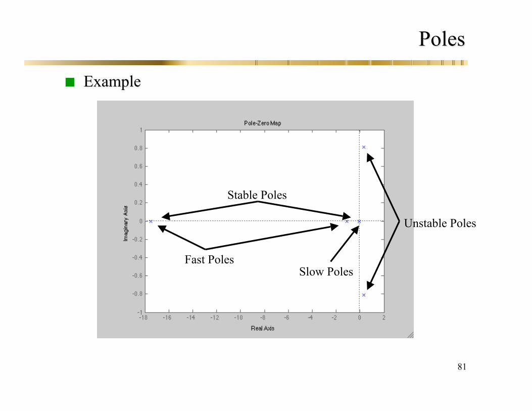
PolesPoles
ExampleExample
Slow Poles
Unstable Poles
Stable Poles
Fast Poles

82
Poles and zeroesPoles and zeroes
Definitions: the roots of are called the zeroszeros of G(s)
the roots of are called the polespoles of G(s)
Zeros: Do not affect the stability of the system but can modify the dynamical
behaviour

83
ZerosZeros
Types of zeros:Types of zeros:
Slow zerosSlow zeros are are closer to the imaginary axis than the dominant poles ofcloser to the imaginary axis than the dominant poles of thethetransfer functiontransfer function Affect the Affect the behaviourbehaviour Results in overshoot (or undershoot)Results in overshoot (or undershoot)
Fast zerosFast zeros are further away to the imaginary axis are further away to the imaginary axis have a negligible impact on have a negligible impact on dynamicsdynamics
Zeros with negative real parts,Zeros with negative real parts, , are , are stable zerosstable zeros Slow stable zeros lead to overshoot Slow stable zeros lead to overshoot
Zeros withZeros with positive real parts,positive real parts, , are , are unstable zerosunstable zeros Slow unstable zeros lead to undershoot (or inverse response) Slow unstable zeros lead to undershoot (or inverse response)

84
ZerosZeros
Can result from two processes in parallel
If gains are of opposite signs and time constants are different then a right halfplane zero occurs
+
+
85
ZerosZeros
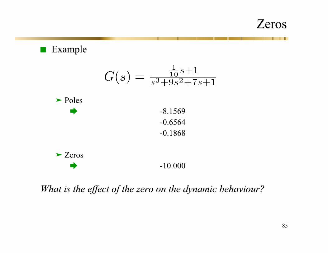
ExampleExample
PolesPoles -8.1569-8.1569
-0.6564-0.6564 -0.1868-0.1868
ZerosZeros -10.000-10.000
What is the effect of the zero on the dynamic What is the effect of the zero on the dynamic behaviourbehaviour??
86
ZerosZeros
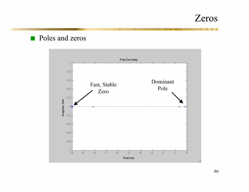
Poles and zerosPoles and zeros
DominantPole
Fast, StableZero
87
ZerosZeros
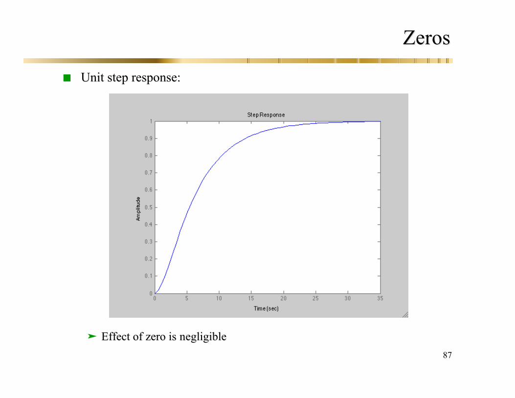
Unit step response:Unit step response:
Effect of zero isEffect of zero is negligiblenegligible
88
ZerosZeros
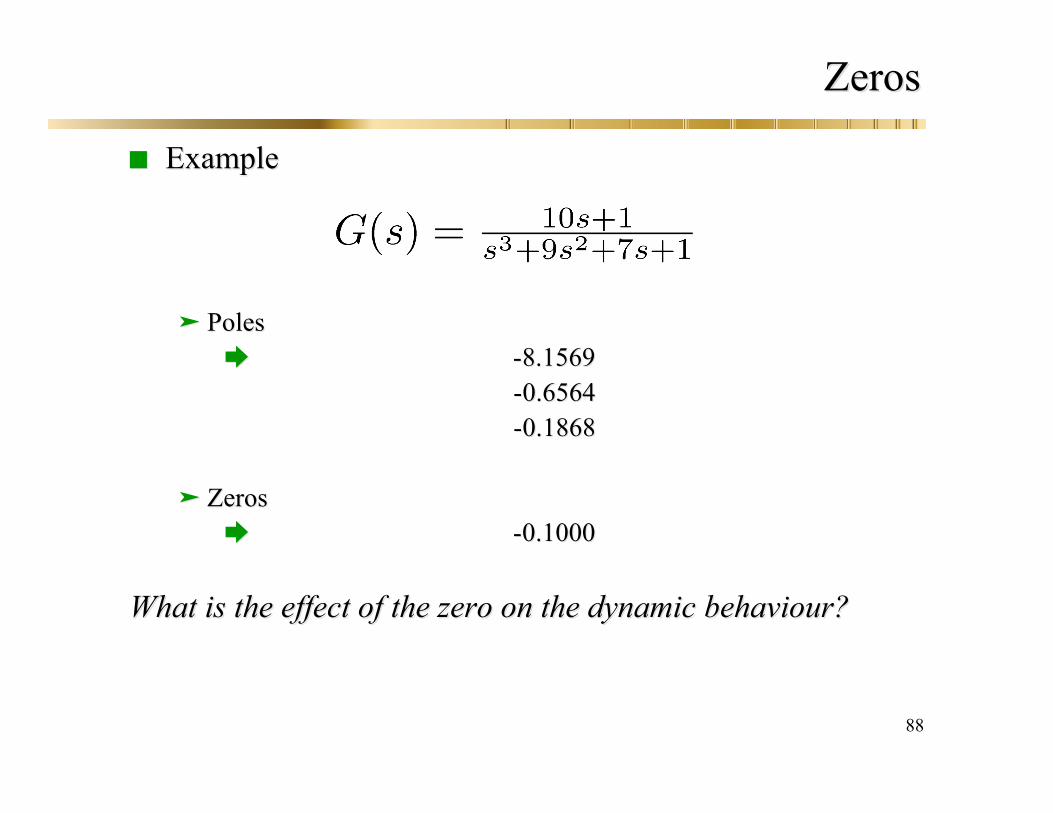
ExampleExample
PolesPoles -8.1569-8.1569
-0.6564-0.6564 -0.1868-0.1868
ZerosZeros -0.1000-0.1000
What is the effect of the zero on the dynamic What is the effect of the zero on the dynamic behaviourbehaviour??

89
ZerosZeros
Poles and zeros:Poles and zeros:
Slow (dominant)Stable zero

90
ZerosZeros
UnitUnit step response:step response:
Slow dominant zeroSlow dominant zero yields an overshoot.yields an overshoot.
91
ZerosZeros
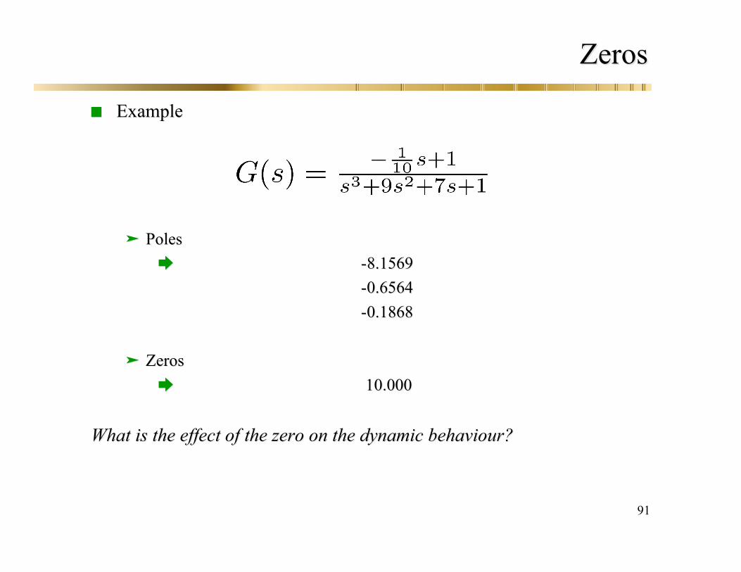
ExampleExample
PolesPoles -8.1569-8.1569
-0.6564-0.6564 -0.1868-0.1868
ZerosZeros 10.00010.000
What is the effect of the zero on the dynamic What is the effect of the zero on the dynamic behaviourbehaviour??
92
ZerosZeros
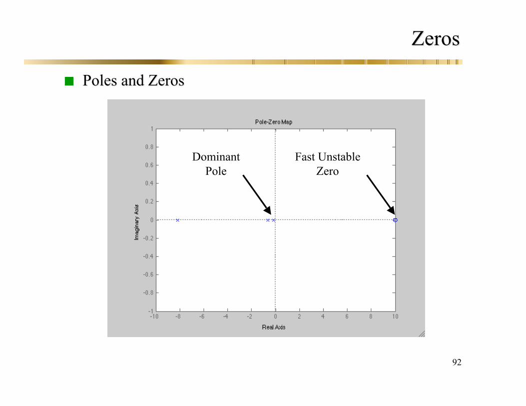
Poles and ZerosPoles and Zeros
Fast UnstableZero
DominantPole

93
ZerosZeros
Unit Step Response:Unit Step Response:
Effect of unstableEffect of unstable zero is negligiblezero is negligible

94
ZerosZeros
ExampleExample
PolesPoles -8.1569-8.1569
-0.6564-0.6564 -0.1868-0.1868
ZerosZeros 0.10000.1000
What is the effect of the zero on the dynamic What is the effect of the zero on the dynamic behaviourbehaviour??
95
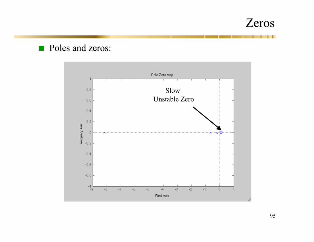
ZerosZeros
Poles and zeros:Poles and zeros:
Slow Unstable Zero
96
ZerosZeros
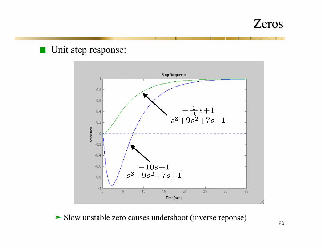
UnitUnit step response:step response:
Slow unstable zero causesSlow unstable zero causes undershoot (inverse undershoot (inverse reponsereponse))
97
ZerosZeros
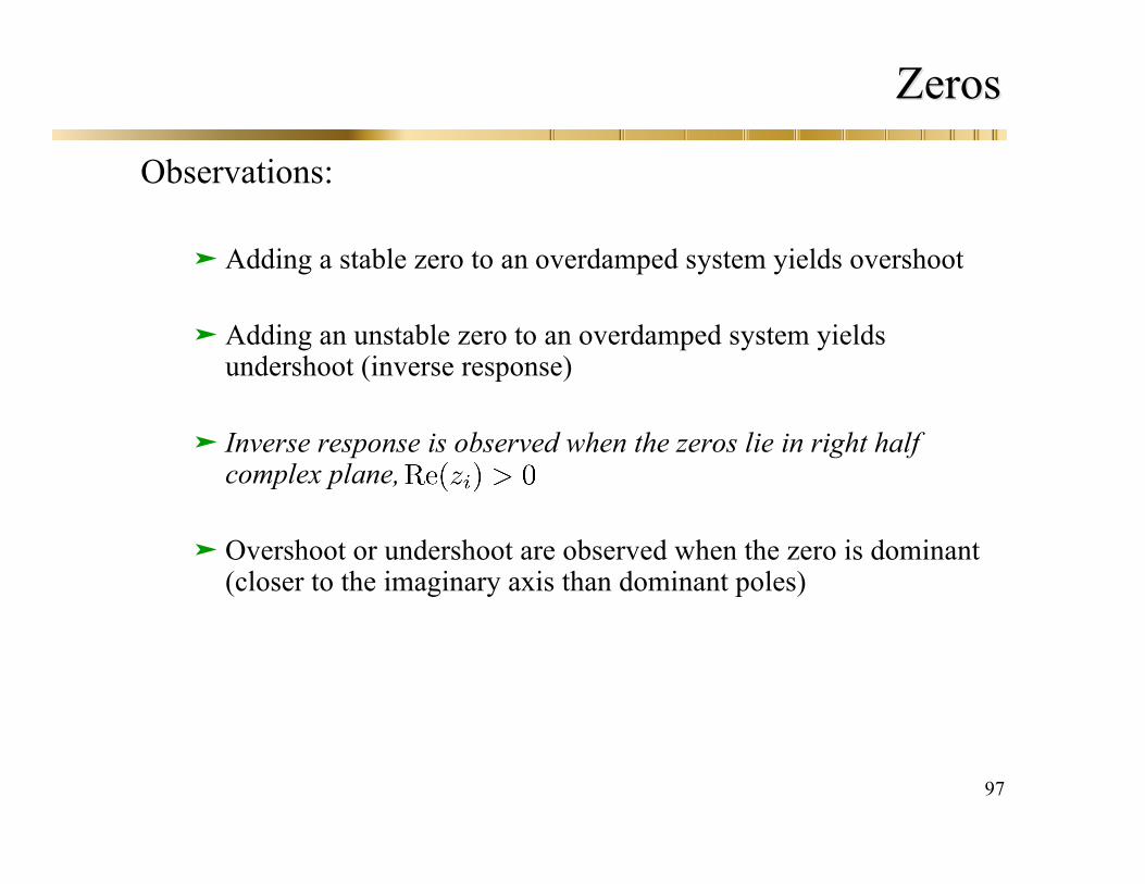
Observations:
Adding a stable zero to an overdamped system yields overshoot
Adding an unstable zero to an overdamped system yieldsundershoot (inverse response)
Inverse response is observed when the zeros lie in right halfcomplex plane,
Overshoot or undershoot are observed when the zero is dominant(closer to the imaginary axis than dominant poles)

98
ZerosZeros
Example: System with complex zerosExample: System with complex zeros
DominantPole
SlowStable Zeros

99
ZerosZeros
Poles and zerosPoles and zeros
PolesPoles havehave negative real parts: The system is stablenegative real parts: The system is stable
Dominant poles are real: yieldsDominant poles are real: yields an an overdamped behaviouroverdamped behaviour
A pair of slow complex stable poles: yields overshootA pair of slow complex stable poles: yields overshoot

100
ZerosZeros
UnitUnit step response:step response:
Effect ofEffect of slow zero is significant and yields oscillatory slow zero is significant and yields oscillatory behaviourbehaviour

101
ZerosZeros
Example: System with zero at theExample: System with zero at the originorigin
Zero atOrigin
102
ZerosZeros
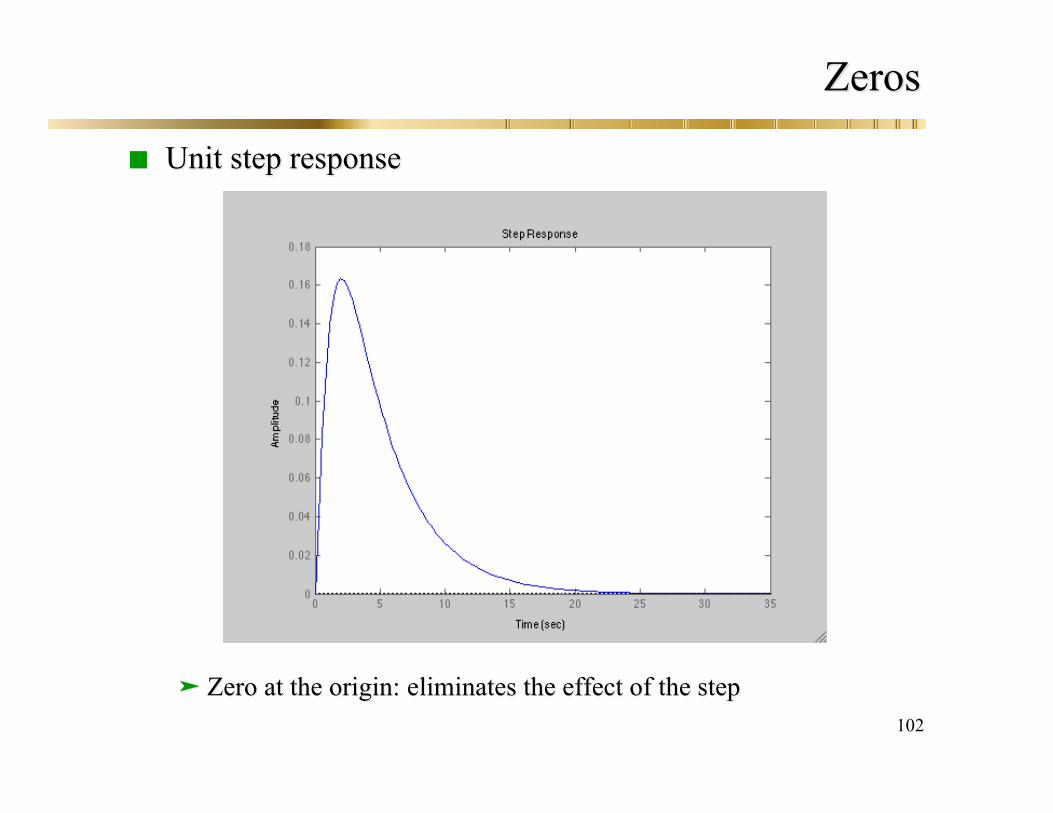
Unit step responseUnit step response
Zero at the origin:Zero at the origin: eliminates the effect of the stepeliminates the effect of the step

103
ZerosZeros
Observations:Observations:
ComplexComplex (stable/unstable) zero that is dominant yields an(stable/unstable) zero that is dominant yields an(overshoot/undershoot)(overshoot/undershoot)
ComplexComplex slow zero can introduceslow zero can introduce oscillatory oscillatory behaviourbehaviour
Zero at the origin eliminates (or zeroes out) the system responseZero at the origin eliminates (or zeroes out) the system response
104
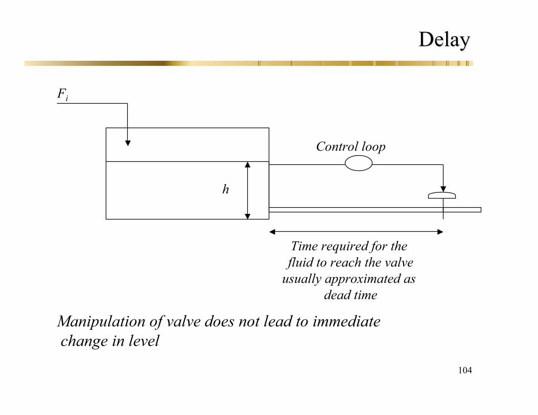
DelayDelay
Time required for the fluid to reach the valve
usually approximated as dead time
h
Fi
Control loop
Manipulation of valve does not lead to immediate change in level

105
DelayDelay
Delayed transfer functions
e.g. First order plus dead-time
Second order plus dead-time
106
DelayDelay
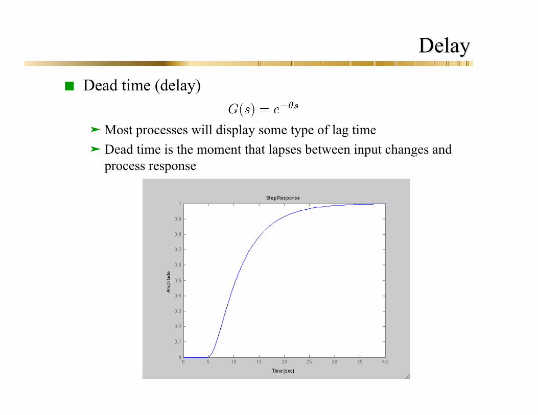
Dead time (delay)
Most processes will display some type of lag timeDead time is the moment that lapses between input changes and
process response
Step response of a first order plus dead time process

107
DelayDelay Delayed step response:Delayed step response:

108
DelayDelay Problem
use of the dead time approximation makes analysis (poles andzeros) more difficult
Approximate dead-time by a rational (polynomial)functionMost common is Pade approximation
109
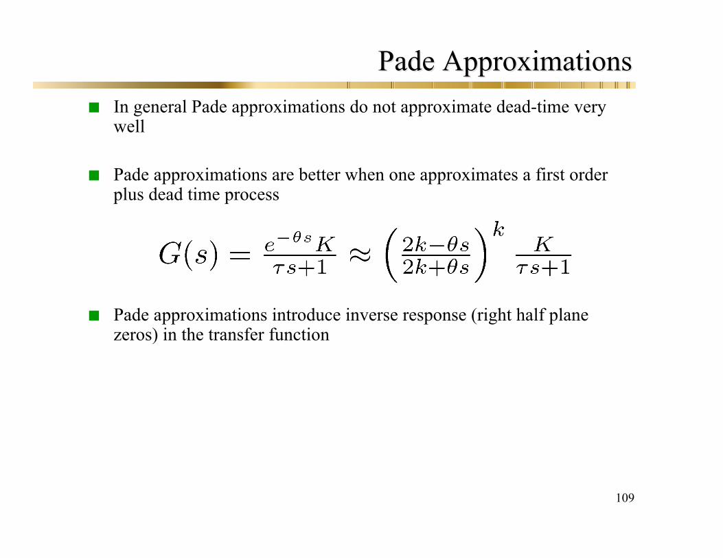
Pade Pade ApproximationsApproximations In general Pade approximations do not approximate dead-time very
well
Pade approximations are better when one approximates a first orderplus dead time process
Pade approximations introduce inverse response (right half planezeros) in the transfer function
110
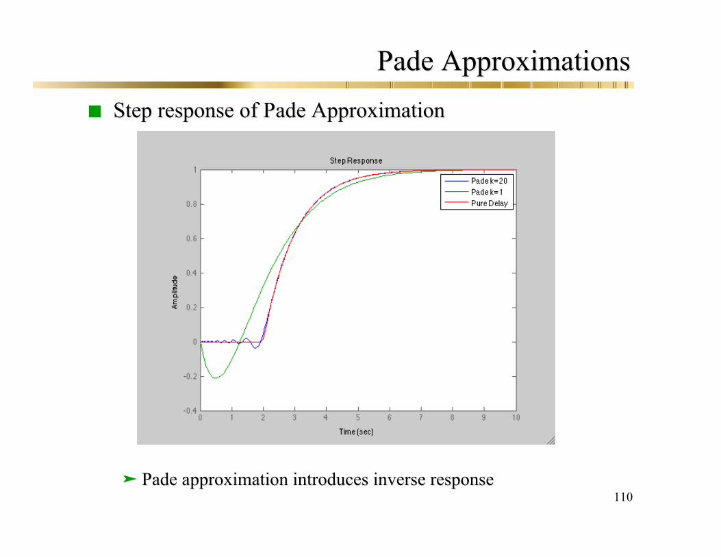
Pade Pade ApproximationsApproximations Step response of Step response of Pade Pade ApproximationApproximation
Pade Pade approximation introduces inverse responseapproximation introduces inverse response