This content has been downloaded from IOPscience. Please scroll down to see the full text.

Download details:

IP Address: 128.114.34.22

This content was downloaded on 11/11/2014 at 23:51

Please note that terms and conditions apply.

Transfer matrix and matrix Green function: the matching problem

View the table of contents for this issue, or go to the journal homepage for more

1990 Phys. Scr. 42 115

(http://iopscience.iop.org/1402-4896/42/1/020)

Home Search Collections Journals About Contact us My IOPscience

Physica Scripta. Vol. 42, 115-123, 1990.

Transfer Matrix and Matrix Green Function: The Matching Problem H. Rodriguez-Coppola,* V. R. Velasco,** F. Garcia-Moliner** and R. PCrez-Alvarez*

*Departamento de Fisica Tebrica, Falcultad de Fisica, Universidad de La Habana, San Lazaro y L, Vedado, La Habana, Cuba; **Institute de Ciencia

@,(4 =

de Materiales, CSIC, Serrano 123, 28006 Madrid, Spain

- 4lI(Z> - -*II(z> - 421 ( z ) *;l(Z>

431(4 = *21(z> .

- 42Ni(Z) - - * ; I (z) -

Received August 4 , 1989; accepted September 26, 1989

Abstract

The connection between the Green function and the transfer matrix is extended beyond the case of one single differential equation - e.g. a one band model. The Surface Green Function Matching analysis is thus per- formed in terms of transfer matrices when the Green functions involved are matrices. The practical use of the formalism is demonstrated by studying two physical problems. One is the spatial analysis of proximity effects associated with elementary excitations in a superconductor in contact with a normal metal or a different superconductor. The other one is a calculation of electronic states in semiconductor superlattices made of lead salts.

1. Introduction

An interesting connection has recently been established [ 1, 21 between Green functions (C) and transfer matrices (M), the latter being defined [3] as matrices which transfer both, wavefunction amplitudes and derivatives. The practical out- come of this is that one can implement the full surface Green function matching (SGFM) analysis to solve the matching problem for one [4] or more [5] interfaces without having to evaluate explicitly the intervening Green functions and their derivatives. This is a considerable practical advantage from the point of view of numerical labour because M can be evaluated by means of efficient numerical algorithms. Thus the full matched Green function of the composite system can be finally obtained explicitly in terms of the inter- vening Ms [2]. One can then easily handle difficult potential profiles which would be practically intractable if one had to evaluate the intervening Cs and their derivatives explicitly. The practical usefulness of this method has been demonstrated by applying it to the study of energy eigenvalues in a semi- conductor parabolic quantum well [ 11, energy eigenvalues and spatial distribution of image potential states on metal surfaces [2] and to a selfconsistent treatment of inversion layers at semiconductor interfaces [2].

In all these cases the mathematical problem involves one differential equation. The problem need not be literally one- dimensional, but crystallinity is definitely excluded, so that by performing a two-dimensional Fourier transform in the (x, y ) plane one introduces a two-dimensional wavevector K but, given that, the mathematical problem is one-dimensional in z as a variable. In view of the practical usefulness of the method it seems desirable to extend it to more realistic, or in any case more complicated, situations.

In problems of physical interest one may find any number N of coupled differential equations, starting with N = 2, as will be seen later. This is significantly different from N = 1 because the Green function then is a 2 x 2 matrix and, with non-commuting objects in the algebra, the analysis needs complete redoing.

The purpose of this paper is to extend the theory beyond N = 1. The formal basis for this is presented in Section 2. Two different physical applications for which N = 2 are given in Sections 3 and 4. This is the first step beyond the scalar case N = 1. The two examples have a physical interest of their own and others can be found. The results thus obtained open the way to an ultimate extension of the appli- cation of a method which may prove practical for to more complicated problems.

116 H . Rodriguez-Coppola, V . R . Velasco, F. Garcia-Moliner and R . PPrez-Alvarez

z’ this leads to

Now, the canonical basis, a term referred to a fixed point zo , is defined by

+fP(z) = 6, for z = zo . (2.5) This is the extension of the case N = 1 studied in Refs. [ l , 21. The purpose of the analysis is to relate G to M and, as in Refs. [ l , 21, this is achieved by choosing the t,bpls of eq. (2.4) to form a canonical basis at zo. This leads finally to the following form of the relationship:

It is convenient to remember the general properties

Thus the derivative of eq. (2.6) from the left is

z / / M 2 p , ] ( z 9 zo)A,,M$ -1./(”> ‘0) ’’;

z ] / M > p - I , , ( z ’ 9 z o ) A , / M $ , / ( z 2 ‘ 0 ) < “ = I (2.8)

aGpp (2, z ‘ ) l3Z

The same remarks made in Refs. [ l , 21 hold here. M is uniquely determined by the differential system, whereas G has so far undetermined parameters A , . One relationship among the A , s is fixed by the jump condition of the derivative. From now on zo will be taken equal to zero without loss of generality and projections at zo = 0 will be indicated by script characters, e.g. 9 is G(0, 0). Defining

(2.9)

and performing a first integration of the differential system one always has

(2.10)

where S is a uniquely determined jump matrix - examples will be seen later. Using eq. (2.10) this yields one condition on the A,s:

AZP,2+ I - A2p-L2p* = Spp,. (2.11)

The rest must be determined by the boundary conditions (BC). For instance, defining

Mi+) = M j j ( + so, O), (2.12)

regularity at - CO, i.e. the BC C ( - CO, 0) = 0, yields

(2.13)

and regularity at + so, i.e., G(0, + m ) = 0, yields

A2p- l , /M&l , / (+) = 0. (2.14) /

Physics Scripra 42

There are 4N2 unknowns A , . The algebraic equations (2.1 l), (2.13), (2.14) yield N 2 conditions each. Thus, 3N2 parameters are so far determined and another N 2 independent conditions are needed. It is easy to see that these can also be obtained from the BCs. For instance, use the SGFM identity

G(z’, Z ) = G(z’, 0) * Y ’G(0, z) , z’ < 0 < z . (2.15)

Differentiate from the right:

a q z ’ , z ) aZ G(z’, z)’ = = G(z’ , 0 ) F ’ - G(0, z)’. (2.16)

Take z + + 0 and z’ + - CO. Then the BC of regularity at - so yields

G ( - “o, Z):=O = G ( - CO, O ) F 1 . G(0, z);-,+O = 0, (2.17)

which, using eq. (2.8) for z’ < z , yields

M > p - I . / ( - ) A ] , 2 p = O‘ (2.18)

This provides the extra needed conditions. Note that eq. (2.18) is different from eq. (2.14). Other BCs may yield dif- ferent results but the analysis is always basically equal. The point is that the last system of N 2 equations is always a consequence of the specified BCs and of an identity and this provides a new system which is neither redundant nor incom- patible. Moreover, the jump condition (2.1 1) is always an inhomogenous system of 4N2 equations for the A , s . In prac- tice these can be found by studying four separate blocks of N 2 parameters each.

In the particular case N = 1 there are four parameters, which are reduced to three by the jump condition

A,, - A , , = S. (2.19)

But the identity (2.15) alone suffices to yield the condition

I

AIlA22 = A,2A2l, (2.20)

which reduces just to three the number of parameters to be determined by (2.19) and by the two BCs. Examination of eq. (2.6) for N = 1 and comparison with eq. (2.4) and eq. (2.3) of Ref. [2] leads in this case to the identification A , = a,Pl and the jump condition (2.19) is the condition (2.9) of Ref. [l]. Thus the case N = 1 is fully recovered from the present analysis. The general relationship (2.6) has the form of a sum of binary products. What makes the case N = 1 unique is that this is the only case for which ( 2 N ) 2 = 2 x 2Nand then the sum of binary products can be reduced to a binary product of sums.

So far for the general relationship between G and M. Now, for any matching problem the analysis proceeds as in Ref. [2], for which the BCs must be specified for each of the two media joined at the matching surface. In order to proceed further it is necessary to define the system under study. We shall con- sider two different cases corresponding to N = 2, both having a physical interest.

3. Application: Elementary excitations in a superconducting

We first consider elementary excitations in superconductors when interfaces are involved. Then the standard BCS theory of a bulk homogeneous medium is not immediately adaptable and, instead, one resorts to alternative formulations. For

b i 1 ay er

Transfer Matrix and Matrix Green Function: The Matching Problem 1 17

temperatures sufficiently different from T, it proves con- venient to start from Bogoliubov’s equations. A normal metal-superconductor interface (N-S) was first studied in this way in Ref. [6] and later in Ref, [7] by using an analytical form of the gap for the superconductor S as a function of position relative to the interface, while in Ref. [8] a constant gap was assumed for S. A normal metal sphere in a super- conducting host was considered in Ref. [9] and a supercon- ducting sphere in a different superconducting host was studied in Ref. [lo]. In both cases the gap was assumed to be constant.

More recently proximity effects in superconducting bilayers (SI - S 2 ) have been studied in Refs. [ l l ] and [12], in both cases starting from Bogoliubov’s equations, the former assuming piecewise constant gaps and the latter introducing into the problem a simplified form of selfconsistency.

The formulation of the problem in principle would be as follows: U(r) is the one-electron potential, A(r) is the pair potential, E is the eigenvalue, measured from the Fermi level EF, u(r) and v(r) are the electron and the hole wavefunctions respectively and Bogoliubov’s equations for a bulk medium are:

[ - & v* - E, + u(r) u,(r ) + ~(r)v , , (v) = ~ , u , ( r ) ; 1 (3.1)

with

The pair potential A(r) should in principle be determined self-consistently by using the condition

(3.3)

where V(r) is the effective attractive potential for electrons and f ( E ) is the Fermi-Dirac function.

The one-electron potential U(r) is usually taken as a con- stant. If desired the mass m could be easily changed into some effective mass m*. For the plane interface problem one Fourier transforms as usual in 2-D, thus introducing the 2-D wavevector K. Then eq. (3.1) becomes a system of two coupled ordinary differential equations in the variable z , perpendicular to the interface. These equations are then K-dependent .

A complete study of the self-consistent problem involving eqs. (3.1) and (3.3) is outside the scope of this paper. Here we are only interested in demonstrating the practical use of the scheme developed in Section 2 to deal with more than one differential equation simultaneously. For this we shall con- sider the simpler situation studied by Yoksan and Nagi [l 11 who took AI and A2 constant and real for the Sl-S2 bilayer. Then for each material the corresponding Bogoliubov’s equations are

(3.4)

h2 d2 (- 2m dzZ - EF U(Z) + AV(Z) = EU(Z);

h2 d2 ( 2m dz2 Au(z) - - - - -

The K-dependence can be understood, in which case E actually stands for E T h2rc2/2m, the - /+ sign holding for u/v, but the focus is on the z-dependent differential equations for which the corresponding matching problem must be solved. Defining the 2-component eigenvector

the system can be compacted into

h2 d2

where

E F - E A

The jump matrix for the Green function corresponding to eq. (3.6) is

2m - h2 = st.

The method discussed in Ref. [3] can be applied to evaluate the transfer matrix M(z, z , ) , discussed here in Section 2. For the system (3.6) the result is given in the Appendix. The problem is then to match two finite layers, one with A = A , , extending from z = a, < 0 to z = 0 and the other one with A = A2 extending from z = 0 to z = a2 > 0. Each medium has the 4 x 4 transfer matrix given in the Appendix, with the corresponding value of A. E, was taken in Ref. [ l l ] to be equal for both media and the same will be done here, although the analysis could be equally done for different values. Each medium has a 2 x 2 matrix Green function G which can be evaluated in terms of its M by applying the analysis developed in Section 2. Then the SGFM analysis can be implemented by writing each G in terms of its own M. This provides the extension to the matrix Green function case N = 2 of the analysis of the scalar Green function given [2] for N = 1.

The boundary conditions must now be prescribed. For the bilayer problem, following [ 1 I ] , we impose the vanishing of the wavefunctions at the ends, z = a, and z = a2, which seems a reasonable BC for the elementary excitations under study, not one-electron states. Consider, for instance, medium 1 on the left. Then eq. (2.13) is replaced by

m2,-,.jAi.2p~-l = 0; m, = M f ) ( a l , 0). (3.9) i

Following the discussion of Refs. [ I , 21 we now choose for medium 1 the second BC at z = 0:

/g(-) = 0. 2 A2p-1.2,’ = 0, (3.10)

whence, from eq. (2.1 I ) which holds in all cases,

A2p.2p,-l = Sppf = sa,, . (3.1 1)

Furthermore, the argument leading from eq. (2.15) to eq. (2.18) can be repeated for medium 1 with - a3 replaced

Physica Scripfa 42

118 H. Rodriguez-Coppola, V. R. Velasco, F. Garcia-Moliner and R. Pdrez-Alvarez

by a , , whence

.i (3.12)

The system (3.9) through (3.12) is easily solved. This yields the A, s for this problem, whence the corresponding Green function (2.6) is readily obtained.

Medium 2, on the right, is studied in the same manner, with mu replaced by nu = Mf’(a2, 0), which transfers to the right. As a second BC at z = 0 we choose - compare with eq. (3.10) -

y(+) = 0. 2 A2,,2p’-l = 0, (3.13)

and the corresponding A,s and Green function are obtained again in the same manner. The choice of BCs (3.10) and (3.13) simplifies the matching formula, which now reads 9-1 = s-1. (q,‘”. 3-1 - ’gC-,.s-l) = 9-1 + 9-1 S 1 2 2 I 2 .

(3.14) The seeular equation is then, simply,

det IY, + Y21 = 0, (3.15)

which in this case yields

m12m33 n12n33

det = 0. (3.16) m34m13 n34n13 m 3 4 m l l n34n11

+ -I -- 62 6, 6 2

Explicit evaluation of eq. (3.16) reproduces very simply the secular equation obtained by Yoksan and Nagi [l l] . These authors calculated the density of states of the bilayer system and found some interesting results which will be commented presently. The evaluation of the density of states from the wavefunctions requires a precise specification of the quantisation scheme employed and the normalisation con- vention adopted, for which the normalisation amplitudes must be obtained. As a general procedure it is rather more straightforward to obtain the density of states, or any other spectral function of interest, directly from the Green function if this can be known. We need only the diagonal part of G, which, for z on side p = 1, 2, is

G,(z, = G,(z, z) + G,(z, 0)

- 3;’ (Ys - 3,) - 9;’ - G,(O, z). (3.17)

All terms entering this formula can be evaluated from eq. (2.6) by using the values of the parameters given above.

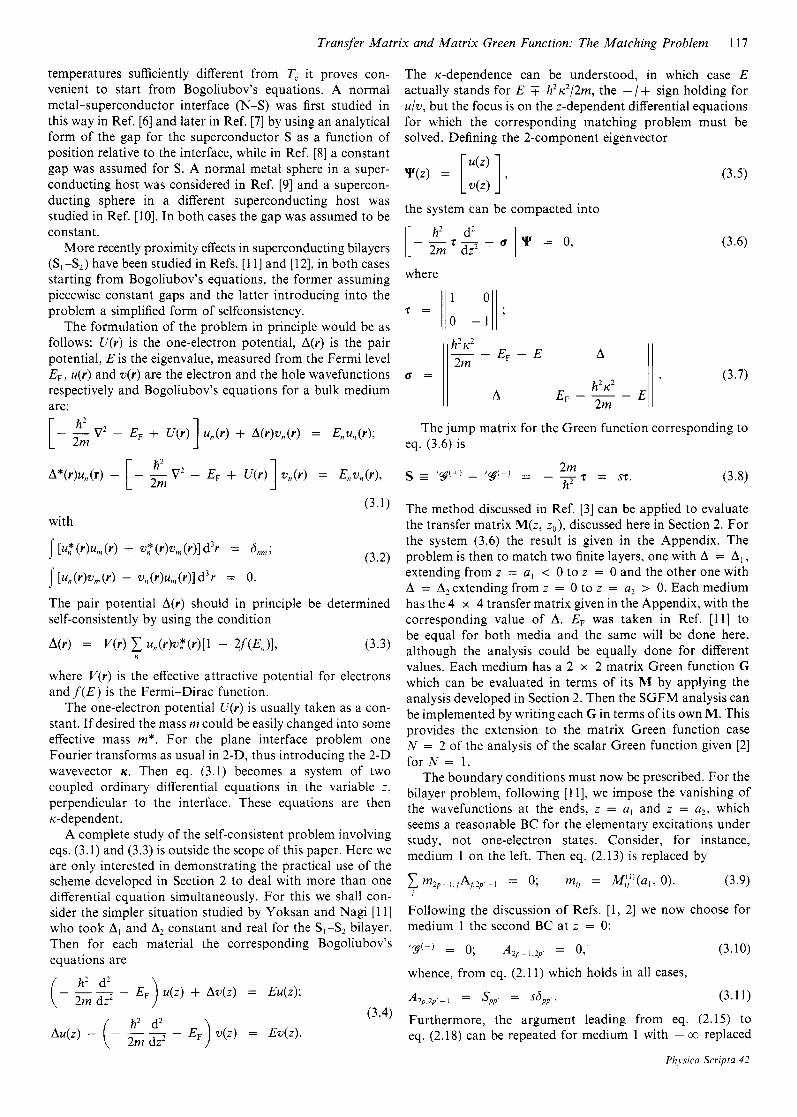
From eq. (3.17) one obtains the local density of states corresponding to a given state {IC, E(Ic)} , while the trace of this yields the total density of states N ( E ) of the bilayer system. Figure 1 shows N ( E ) for thick layers (lalI = a2 = 305, 5 = coherence length in S , ) for A, = 0 and o .4A2 , first obtained in Ref. [ l l ] and corroborated in the present calculation. The result for A, = 0.4A2 shows the usual BCS peak at the threshold energy E = A , . Starting at E = A2 there is another, and stronger, BCS peak, not shown in the figure. The interesting result is that there is some spectral strength at all energies for A, = 0, - full line in Fig. 1. This type of proximity effect was first pointed out in Ref. [6] for lu, I = 35, and it is also manifest for a much thicker normal layer, with 14, I = 305. The curve N ( E ) looks like a sort of small BCS peak, as if the normal metal layer

Physica Scripta 42

I O 0

8.0

6 0

w z Y

4.0

20

I 1 I

0.0 0.5 I .o

E/&

Fig. 1 . Elementary excitations in Bogoliubov’s model for superconductors in a bilayer. Layer 2 is a superconductor with gap A2, coherence length 5 and thickness 305. Layer 1 has also thickness 305 while A , = 0 (normal metal) for the full line and A , = 0.4 for the dashed line.

became, by proximity effect, something like a nearly zero gap superconductor.

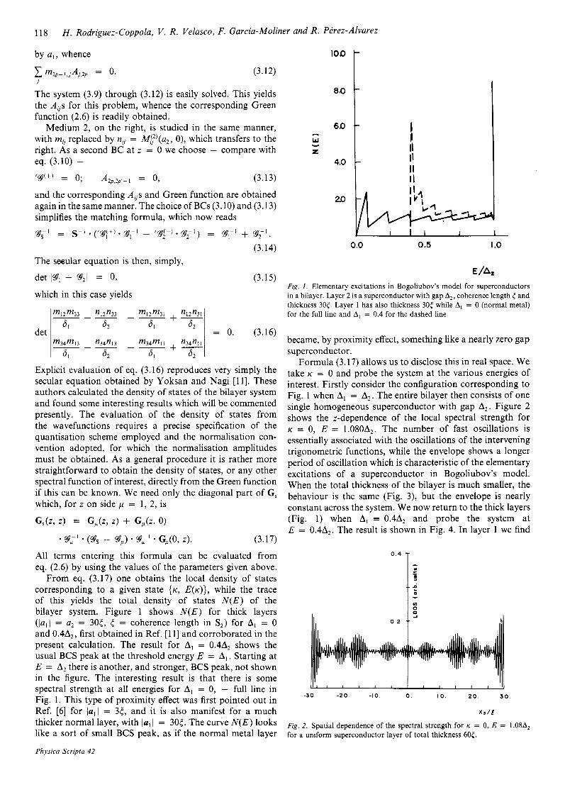
Formula (3.17) allows us to disclose this in real space. We take IC = 0 and probe the system at the various energies of interest. Firstly consider the configuration corresponding to Fig. 1 when A, = A2, The entire bilayer then consists of one single homogeneous superconductor with gap A2. Figure 2 shows the z-dependence of the local spectral strength for IC = 0, E = 1.0806,. The number of fast oscillations is essentially associated with the oscillations of the intervening trigonometric functions, while the envelope shows a longer period of oscillation which is characteristic of the elementary excitations of a superconductor in Bogoliubov’s model. When the total thickness of the bilayer is much smaller, the behaviour is the same (Fig. 3), but the envelope is nearly constant across the system. We now return to the thick layers (Fig. 1) when A, = 0.4A2 and probe the system at E = 0.4A2. The result is shown in Fig. 4. In layer 1 we find

1 1 1

0.2 1; I l l

( I , I I I I , I 1 , , , , I)

-3 0 -20 -10. 0 . I O . 20. 30

xr/C

Fig. 2. Spatial dependence of the spectral strength for K = 0, E = 1.08A2 for a uniform superconductor layer of total thickness 605.

Transfer Matrix and Matrix Green Function: The Matching Problem 119

- .I

c c

4 - v) 0

-1 a

-3 . - 2 . 5 - 2 . -1.5 - 1 . -0.5 0. 0.3

T I .

-- 0 .8

-- 0 . 6

-- 0.4

X. /C

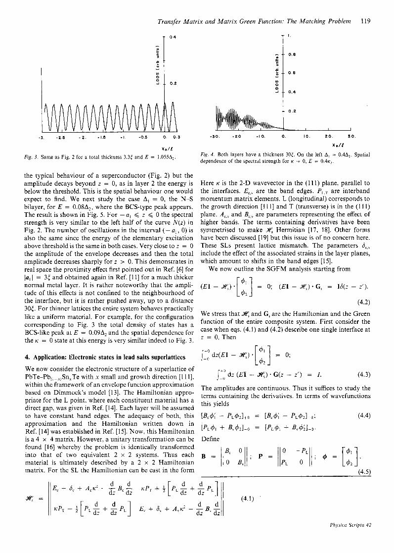
Fig. 3. Same as Fig. 2 for a total thickness 3.35 and E = 1.05SA2.

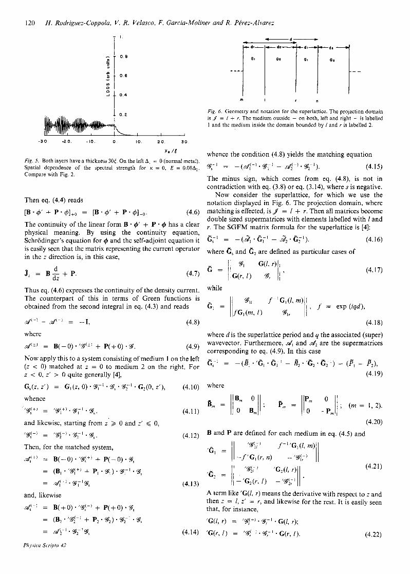
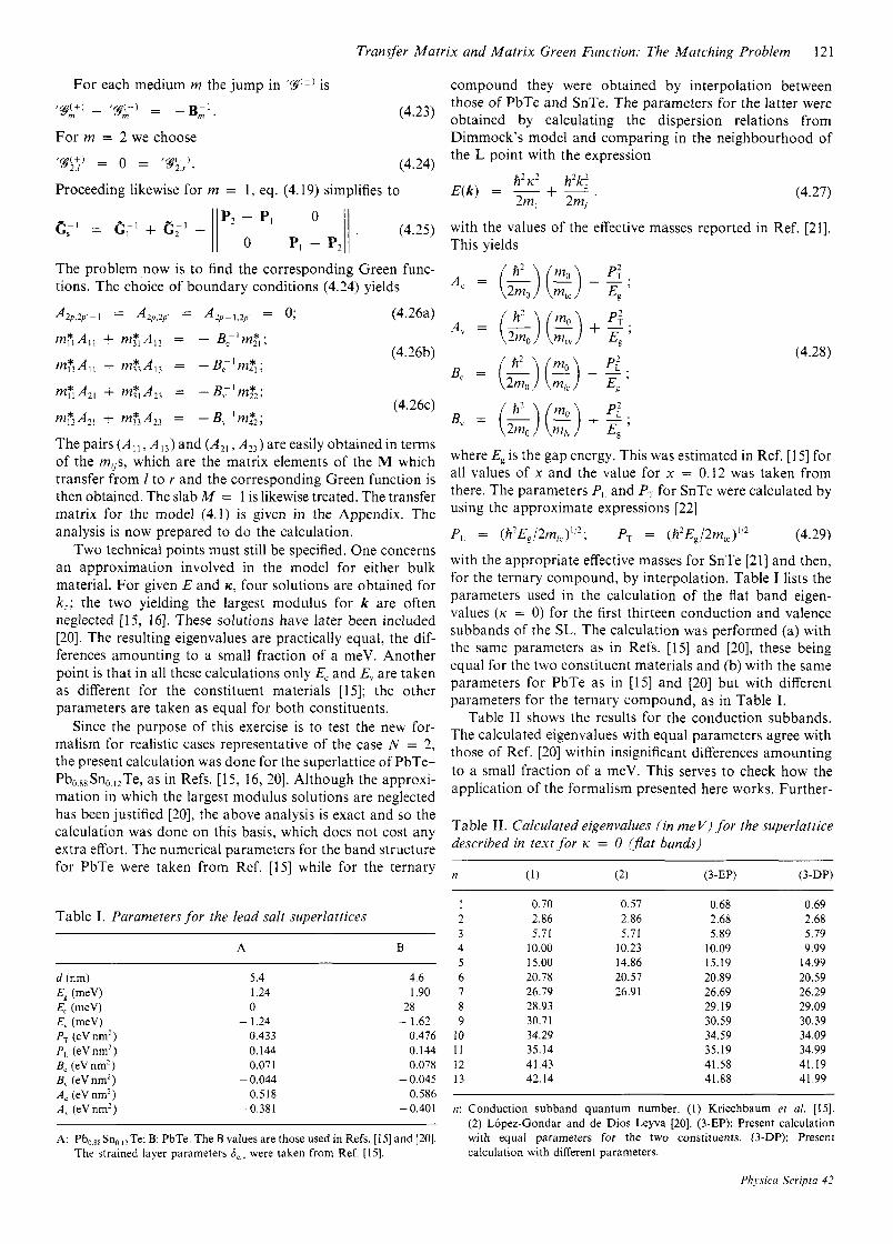
the typical behaviour of a superconductor (Fig. 2) but the amplitude decays beyond z = 0, as in layer 2 the energy is below the threshold. This is the spatial behaviour one would expect to find. We next study the case Al = 0, the N-S bilayer, for E = 0.08A2, where the BCS-type peak appears. The result is shown in Fig. 5. For -al < z < 0 the spectral strength is very similar to the left half of the curve N(z) in Fig. 2. The number of oscillations in the interval (- a , , 0) is also the same since the energy of the elementary excitation above threshold is the same in both cases. Very close to z = 0 the amplitude of the envelope decreases and then the total amplitude decreases sharply for z > 0. This demonstrates in real space the proximity effect first pointed out in Ref. [6] for lal I = 35 and obtained again in Ref. [l 11 for a much thicker normal metal layer. It is rather noteworthy that the ampli- tude of this effects is not confined to the neighbourhood of the interface, but it is rather pushed away, up to a distance 305. For thinner lattices the entire system behaves practically like a uniform material. For example, for the configuration corresponding to Fig. 3 the total density of states has a BCS-like peak at E = 0.09A2 and the spatial dependence foir the K = 0 state at this energy is very similar indeed to Fig. 3.

4. Application: Electronic states in lead salts superlattices

We now consider the electronic structure of a superlattice of PbTe-Pb,, - ,,Sn,Te with x small and growth direction [ 11 13, within the framework of an envelope function approximation based on Dimmock's model [13]. The Hamiltonian appro- priate for the L point, where each constituent material has a direct gap, was given in Ref. [14]. Each layer will be assumed to have constant band edges. The adequacy of both, this approximation and the Hamiltonian written down in Ref. [14] was established in Ref. [15]. Now, this Hamiltonian is a 4 x 4 matrix. However, a unitary transformation can be found [ 161 whereby the problem is identically transformed into that of two equivalent 2 x 2 systems. Thus each material is ultimately described by a 2 x 2 Hamiltonian matrix. For the SL the Hamiltonian can be cast in the form

0 . I O . 2 0 . 30 -30. -20. -IO.

X I / [

Fig. 4. Both layers have a thickness 305. On the left A, = 0.4A2. Spatial dependence of the spectral strength for K = 0, E = 0 . 4 ~ ~ .

Here ti is the 2-D wavevector in the (1 11) plane, parallel to the interfaces. EC,, are the band edges. P L , T are interband momentum matrix elements. L (longitudinal) corresponds to the growth direction [l 1 11 and T (transverse) is in the (1 11) plane. A , , and BC,, are parameters representing the effect of higher bands. The terms containing derivatives have been symmetrised to make &s Hermitian [17, 181. Other forms have been discussed [19] but this issue is of no concern here. These SLs present lattice mismatch. The parameters 6 , , include the effect of the associated strains in the layer planes, which amount to shifts in the band edges [15].

(E1 - &)-[ ::] = 0; (E1 - Yi",).G, = I6(z - z').

We now outline the SGFM analysis starting from

(4 * 2) We stress that .yt4 and G , are the Hamiltonian and the Green function of the entire composite system. First consider the case when eqs. (4.1) and (4.2) describe one single interface at z = 0. Then

I:," dz (E1 - e) * G(z - z') = I . (4.3)

The amplitudes are continuous. Thus it suffices to study the terms containing the derivatives. In terms of wavefunctions this yields

P c 4 ; - P L 4 2 1 , O = tBC4 - P L 4 2 1 - 0 ; (4.4)

P L 4 I + B"421+0 = P L 4 I + 44; I -o . Define

(4.5)

(4.1)

d d dz dz E, + 6, + A c ~ 2 - - B, - K P ~ + 3

E, + 6, + A,ti2 - - B, - 2 q =

d d dz dz

Physica Scr ip ia 4 2

120 H. Rodriguez-Coppola, V. R. Velasco, F. Garcia-Moliner and R . Pbez-Alvarez

T i

-30. - 2 0 . -10. 0. I O . 2 0. 30.

X a / E

Fig. 5. Both layers have a thickness 30t;. On the left A, = 0 (normal metal). Spatial dependence of the spectral strength for K = 0, E = 0.08A2. Compare with Fig. 2.

Then eq. (4.4) reads

[B 4' + P * 4]+0 = [B 4' + P * 4 3 - 0 . (4.6) The continuity of the linear form B - 4' + P - 4 has a clear physical meaning. By using the continuity equation, Schrodinger's equation for 4 and the self-adjoint equation it is easily seen that the matrix representing the current operator in the z direction is, in this case,

(4.7) d dz

3: = B - + P .

Thus eq. (4.6) expresses the continuity of the density current. The counterpart of this in terms of Green functions is obtained from the second integral in eq. (4.3) and reads

&#+) - d(-) =

where - I, (4.8)

+ P(+O) -3. (4.9) d(" = B(+O) . Now apply this to a system consisting of medium 1 on the left ( z < 0) matched at z = 0 to medium 2 on the right. For z < 0, z' > 0 quite generally [4],

G,(z, z ' ) = G I ( z , 0 ) %ri - 9, - 9;' * G2(0, z ' ) , (4.10)

whence

v$+) = /@+I. 1 8;' . 9,. (4.1 1)

and likewise, starting from z > 0 and z' < 0,

q-i-1 = .y(-).g-l 2 . % S . (4.12)

Then, for the matched system,

4") = B(-0) '3J+) + P(- 0) *

= (B, * '%!+I + PI - 3,) - 3,' - gS

= d/+J . % - I % I s (4.13)

and, likewise

4(-) = B(+ 0) - '9J-J + P(+O) gS

=

= &I-) .gj;'g, (4.14)

(B2 * '%j-) + P, * g2) * 3;' * gS

Physica Scripta 42

m I r n

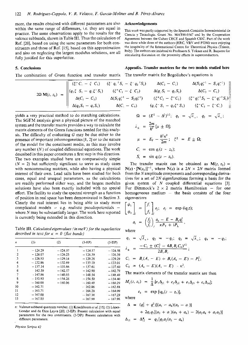
Fig. 6. Geometry and notation for the superlattice. The projection domain is = I + 1. The medium outside - on both, left and right - is labelled 1 and the medium inside the domain bounded by I and r is labelled 2.

whence the condition (4.8) yields the matching equation

%,-I = -(d(+J.%-I I - & ( - ) . % - I ) 2 2 . (4.15)

The minus sign, which comes from eq. ( 4 . Q is not in contradiction with eq. (3.8) or eq. (3.14), where s is negative.

Now consider the superlattice, for which we use the notation displayed in Fig. 6. The projection domain, where matching is effected, is 3 = I + r. Then all matrices become double sized supermatrices with elements labelled with I and r. The SGFM matrix formula for the superlattice is [4]:

G-1 = -@,. - &&. (?&I)* (4.16)

where e, and e2 are defined as particular cases of

(4.17)

while

(4.18)

where d is the superlattice period and q the associated (super) wavevector. Furthermore, d, and d2 are the supermatrices corresponding to eq. (4.9). In this case

e;1 = -(B1 - 'Cl * C;l - B2 '(2, ' e;') - (p", - F2), (4.19)

where

(4.20) B and P are defined for each medium in eq. (4.5) and

(4.21)

A term like 'G(1, r ) means the derivative with respect to z and then z = I , z' = r, and likewise for the rest. It is easily seen that, for instance,

(4.22)

Transfer Matrix and Matrix Green Function: The Matching Problem 12 1

For each medium m the jump in '@*I is

m (4.23) '@JrJ - = -B;1.

For m = 2 we choose

'@J$;J = 0 = '9c-J. 2.r (4.24)

Proceeding likewise for m = 1, eq. (4.19) simplifies to

The problem now is to find the corresponding Green func- tions. The choice of boundary conditions (4.24) yields

A2p,Zp,-1 = A2p,2p' = A2p-1,2p. = 0; (4.26a)

m?,A,, + m,*,A,, = - B;'m,*,;

mT3Al, + m,*,A,, = -B;'m,*,;

m;C,A,, + m,*,A,, = -B;'m,*,;

mT3A2, + m,*,A,, = - B;'m,*,;

(4.26b)

(4.26~)

The pairs (All , A ' , ) and (A2l, A2,) are easily obtained in terms of the m,s, which are the matrix elements of the M which transfer from 1 to r and the corresponding Green function is then obtained. The slab M = 1 is likewise treated. The transfer matrix for the model (4.1) is given in the Appendix. The analysis is now prepared to do the calculation.

Two technical points must still be specified. One concerns an approximation involved in the model for either bulk material. For given E and K, four solutions are obtained for k, ; the two yielding the largest modulus for k are often neglected [15, 161. These solutions have later been included [20]. The resulting eigenvalues are practically equal, the dif- ferences amounting to a small fraction of a meV. Another point is that in all these calculations only E, and E, are taken as different for the constituent materials [ 151; the other parameters are taken as equal for both constituents.

Since the purpose of this exercise is to test the new for- malism for realistic cases representative of the case .N = 2, the present calculation was done for the superlattice of PbTe- Pb,,,Sn, ,,Te, as in Refs. [15, 16, 201. Although the approxi- mation in which the largest modulus solutions are neglected has been justified [20], the above analysis is exact and so the calculation was done on this basis, which does not cost any extra effort. The numerical parameters for the band structure for PbTe were taken from Ref. [15] while for the ternary

Table I. Parameters for the lead salt superlattices

A B

5.4 1.24 0

- 1.24 0.433 0.144 0.071

0.518 - 0.044

-0.381

4.6 1.90

28 - 1.62

0.476 0.144 0.078

0.586 - 0.045

- 0.401

A: Pb,,,Sn, ,>Te; B: PbTe. The B values are those used in Refs. [IS] and [20]. The strained layer parameters hC," were taken from Ref. [15].

compound they were obtained by interpolation between those of PbTe and SnTe. The parameters for the latter were obtained by calculating the dispersion relations from Dimmock's model and comparing in the neighbourhood of the L point with the expression

h ' ~ ' h2k! 2m, 2m,

E(k) = - + - . (4.27)

with the values of the effective masses reported in Ref. [21]. This yields

A, = ( $ ) ( $ ) - E , . p: .

A , = (&)(?)+-; P:

EP

p: .

B, = (d)($)+s; (4.28)

where Eg is the gap energy. This was estimated in Ref. [ 151 for all values of x and the value for x = 0.12 was taken from there. The parameters P, and PT for SnTe were calculated by using the approximate expressions [22]

P, = (h'EJ2n~,~)'~'; P, = (Z12Eg/2m,,)''2 (4.29)

with the appropriate effective masses for SnTe [21] and then, for the ternary compound, by interpolation. Table I lists the parameters used in the calculation of the flat band eigen- values (ti = 0) for the first thirteen conduction and valence subbands of the SL. The calculation was performed (a) with the same parameters as in Refs. [15] and [20], these being equal for the two constituent materials and (b) with the same parameters for PbTe as in [I51 and [20] but with different parameters for the ternary compound, as in Table I.

Table I1 shows the results for the conduction subbands. The calculated eigenvalues with equal parameters agree with those of Ref. [20] within insignificant differences amounting to a small fraction of a meV. This serves to check how the application of the formalism presented here works. Further-

Table 11. Calculated eigenvalues (in me V ) for the superlattice described in text for K = 0 (flat bands)

~

n (1) (2) (3-EP) (3-DP)

1 2 3 4 5 6 I 8 9

10 11 12 13

0.70 2.86 5.71

10.00 15.00 20.78 26.79 28.93 30.71 34.29 35.14 41.43 42. I4

0.57 0.68 2.86 2.68 5.71 5.89

10.23 10.09 14.86 15.19 20.57 20.89 26.91 26.69

29.19 30.59 34.59 35.19 41.58 41.88

0.69 2.68 5.79 9.99

14.99 20.59 26.29 29.09 30.39 34.09 34.99 41.19 41.99

n: Conduction subband quantum number. ( I ) Kriechbaum et al. [15]. (2) L6pez-Gondar and de Dios Leyva [20]. (3-EP): Present calculation with equal parameters for the two constituents. (3-DP): Present calculation with different parameters.

Physica Scripla 42

122 H . Rodriguez-Coppola, V . R . Velasco, F. Garcia-Moliner and R . PPrez-Alvarez

more, the results obtained with different parameters are also within the same range of differences, i.e. they are equal in practice. The same observations apply to the results for the valence subbands, shown in Table 111. Thus the calculation of Ref. [20], based on using the same parameters for both con- stituents and those of Ref. [15], based on this approximation and also on neglecting the largest modulus solutions, are all fully justified for this superlattice.

5. Conclusions

The combination of Green function and transfer matrix - 1 1 (t:c, - 5-C3) ( t+4F1SI

Acknowledgements This work was partly supported by the Spanish Comisi6n Interministerial de Ciencia y Tecnologia, Grant No. MAT88-0547 and by the Cooperation Agreement between the Cuban CECE and Spanish CSIC. Part of the work was done while three of the authors (HRC, VRV and FGM) were enjoying the hospitality of the International Centre for Theoretical Physics (Trieste, Italy). The authors are indebted to Professors S . Yoksan and R. Baquero for stimulating discussion on the proximity effects in superconductors.

Appendix. Transfer matrices for the two models studied here

The transfer matrix for Bogoliubov's equations is

yields a very practical method to do matching calculations. The SGFM analysis gives a physical picture of the matched system and the transfer matrix provides a way to calculate the matrix elements of the Green functions needed for this analy- sis. The difficulty of evaluating G may be due either to the presence of important inhomogeneities [ l , 21 or to the nature of the model for the constituent media, as this may involve any number ( N ) of coupled differential equations. The work described in this paper constitutes a first step in this direction. The two examples studied here are comparatively simple ( N = 2) but sufficiently significant to serve as study cases with noncommuting matrices, while also having a physical interest of their own. Lead salts have been studied for both cases, equal and unequal parameters, as the calculations are readily performed either way, and the largest modulus solutions have also been exactly included with no special effort. The facility to study the spectral strength as a function of position in real space has been demonstrated in Section 3. Clearly the real interest lies in being able to study more complicated models - e.g. realistic pseudopotentials - where N may be substantially larger. The work here reported is currently being extended in this direction.

Table 111. Calculated eigenvalues (in me V ) for the superlattice described in text for IC = 0 ('at bands)

n (1) (2) (3-EP) (3-DP)

1 - 124.29 - 124.57 - 124.57 - 124.58 2 - 126.07 - 126.23 - 126.39 - 126.39 3 - 128.93 - 129.14 - 129.28 - 129.29 4 - 132.86 - 132.69 - 133.10 - 133.01 5 - 137.14 - 135.66 - 137.61 - 137.60 6 - 142.50 - 142.57 - 142.90 - 142.79 7 - 147.86 - 148.03 - 148.54 - 148.49 8 - 153.93 - 154.26 - 154.50 - 154.40 9 - 160.00 - 160.06 - 160.49 - 160.29

10 - 162.71 - 162.86 - 162.88 11 - 163.71 - 164.20 - 164.09 12 - 167.00 - 167.38 - 167.29 13 - 167.85 - 167.99 - 167.98

n: Valence subband quantum number. (1) Kriechbaum et al. [15]. (2) Lopez- Gondar and de Dios Leyva [20]. (3-EP): Present calculation with equal parameters for the two constituents. (3-9P): Present calculation with different parameters.

Physiea Scripta 42

2m 212 [P f QI;

cos qi(z - zo);

sin qi(z - zo).

E L Q;

The transfer matrix can be obtained as M ( z , z o ) = N(z) - [N(z , ) ] - ' , where N(z ) is a 2N x 2N matrix formed from the N amplitude components and corresponding deriva- tives for a set of 2N eigenfunctions forming a basis for the given system of N coupled differential equations [3]. For Dimmock's 2 x 2 matrix Hamiltonian - for one homogeneous medium - the basis consists of the four eigenvectors

[ '11 = ["I ej; e, = exp (iqjz); '2 j f 2 j

Transfer Matrix and Matrix Green Function: The Matching Problem 123

19. Perez-Alvarez, R., Rodriguez-Coppola, H., Velasco, V. R. and 20, Garcia-Moliner, F., J. Phys. C: Solid State Phys. 21, 2197 (1988). Velasco, V. R., Garcia-Moliner, F., Rodriguez-Coppola, H. and 21,

22 Perez-Alvarez, R., Physica Scripta 41, 375 (1989). Mora, M., Perez-Alvarez, R. and Sommers, Ch. B., J. Physique 46, 1021 (1985).

Garcia-Moliner, F. and Rubio, J., Proc. Roy. Soc. London A234, 257 (1 97 1). Garcia-Moliner, F. and Velasco, V. R., Surf. Sci. 175, 9 (1986). De Gennes, P. G. and Saint-James, D., Phys. Lett. 4, 151 (1963). Bar-Sagi, J., Solid St. Commun. 27, 363 (1978). Zaitlin, M. P., Phys. Rev. B25, 5729 (1982). Hui, P. M. and Stroud, D., Phys. Rev. B31, 584 (1985). Yoksan, S. and Nagi, A. D. S . , Solid St. Commun. 56, 763 (1985). Yoksan, S. and Nagi, A. D. S., J. Low Temp. Phys. 66, 115 (1987). Kobes, R. L. and Whitehead, J. P., Phys. Rev. 836, 121 (1987). Dimmock, J . O., Proc. Conf. Physics of Semimetals and Narrow gap Semiconductors, p. 319. Dallas, U.S.A. (1970). Bauer, G., Narrow Gap Semiconductor Physics and Applications (Edited by W. Zawadzki), Lecture Notes in Physics, Vol. 133, p. 427. Springer Verlag, Berling (1980). Kriechbaum, M., Ambrosch, K. E., Fantner, E. J., Clemens, H. and Bauer, G., Phys. Rev. B30, 3394 (1984). De Dios Leyva, M. and Lopez-Gondar, J., Phys. Stat. Solidi (b) 138, 253 (1986). Enders, P., Phys. Stat. Solidi (b) 139, KI 13 (1987). Potz, W. and Ferry, D. K., Superlattices and Microstructures 3, 57 ( 1987). Morrow, R. A., Phys. Rev. B35, 8074 (1987). Lopez-Gondar, J. and de Dios Leyva, M., Phys. Stat. Solidi (b) 142, 445 (1987). Bernick, R. L. and Kleinman, L., Solid. St. Commun. 8, 569 (1970). Bastard, G., Phys. Rev. B25, 7584 (1982).

Physica Scripta 4 2