TRANSIENT DETECTION AND MODELING OF

CONTINUOUS GEODETIC DATA

A Thesis

Presented to

The Graduate Faculty

Central Washington University

In Partial Fulfillment

of the Requirements for the Degree

Master of Science

Geology

by

Walter Michael Szeliga

November 2005

CENTRAL WASHINGTON UNIVERSITY

Graduate Studies

We hereby approve the thesis of

Walter Michael Szeliga

Candidate for the degree of Master of Science

APPROVED FOR THE GRADUATE FACULTY

Dr. Timothy Ian Melbourne, Committee Chair

Dr. M. Meghan Miller

Dr. Jeffrey Lee

Associate Vice President of Graduate Studies

ii

ABSTRACT

TRANSIENT DETECTION AND MODELING OF

CONTINUOUS GEODETIC DATA

by

Walter Michael Szeliga

November 2005

Transient surface deformation has been observed by continuously operating

Global Positioning System stations in the Puget Sound area during the past decade. This

surface deformation is associated with processes occurring on or near the subducting plate

boundary between the Juan de Fuca and North American plates. This thesis is composed

of two studies of transient deformation along the Cascadia plate margin and a discussion

of the methodologies employed in these studies. We model one 7-week episode of

transient deformation that occurred during 2003 beneath the Puget Sound area.

Additionally, we utilize a combination of continuous Global Positioning System and

seismic data to provide evidence for the occurrence of transient deformation in southern

Cascadia. The remainder of the thesis focuses on the methodologies utilized in both

identifying and modeling these episodes of transient deformation.

iii

ACKNOWLEDGMENTS

While the research required for this thesis has been supported by numerous people

and organizations, the first three chapters deserve specific mention.

Research for the chapter titled “Southern Cascadia Episodic Slow Earthquakes”

was supported by National Science Foundation grant EAR-0208214, U.S. Geological

Survey National Earthquake Hazards Reduction Program (NEHRP) award 04HQGR0005,

the National Aeronautics and Space Administration grant SENH-0000-0264, and Central

Washington University (CWU). Global Positioning System (GPS) data collection was

supported by the National Science Foundation under grant EAR-0318549 to UNAVCO,

Inc., and grants EAR-0002066 and EAR-9616540 to CWU; by the National Aeronautics

and Space Administration NASA contracts NAG5-13728 and NAG5-7672; and by the

U.S. Geological Survey NEHRP award 04HQAG0007 and CWU. I would like to thank

Craig Scrivner (of CWU) for discussion and help with software needed for automated

downloading and viewing of Northern California Seismic Network seismic data in record

section format, the Pacific Northwest Geodetic Array (PANGA), the Western Canadian

Deformation Array operated by the Pacific Geoscience Centre for the Geological Survey

of Canada, the Scripps Institute of Oceanography, the Northern California Earthquake

Data Center, the Northern California Seismic Network, U.S. Geological Survey, Menlo

Park and the Berkeley Seismological Laboratory, University of California, Berkeley for

GPS and seismic time series.

Research for the chapter titled “Extent and Duration of the 2003 Cascadia Slow

Earthquake” was supported by National Science Foundation grant EAR-0208214, U.S.

Geological Survey NEHRP award 04HQGR0005, the National Aeronautics and Space

Administration grant SENH-0000-0264, and CWU. GPS data collection was supported by

the National Science Foundation under grants EAR-0318549 to UNAVCO, Inc., and

iv

grants EAR-0002066 and EAR-9616540 to CWU; by the National Aeronautics and Space

Administration NASA contracts NAG5-13728 and NAG5-7672; and by the U.S.

Geological Survey NEHRP award 04HQAG0007 and CWU. I would like to thank the

PANGA and the Western Canadian Deformation Array operated by the Pacific

Geoscience Centre of the Geological Survey of Canada for use of their data.

Research for the chapter titled “QRfit, A Flexible Utility for Time Series

Decomposition” was supported by National Science Foundation grant EAR-0208214,

U.S. Geological Survey NEHRP award 04HQGR0005, the National Aeronautics and

Space Administration grant SENH-0000-0264, CWU, and by the U.S. Geological Survey

NEHRP award 04HQAG0007.

Research for the chapter titled “GPS Inversion with Positivity Constraints” was

supported by the National Science Foundation under grants EAR 0318549 to UNAVCO,

Inc., and grants EAR-0002066 and EAR-9616540 to CWU; by the National Aeronautics

and Space Administration NASA contracts NAG5-13728 and NAG5-7672 to CWU; and

by the U.S. Geological Survey NEHRP award 04HQAG0007 to CWU. Observations are

also supported by member institutions of the PANGA consortium. Additionally, I would

like to thank Dr. Per Christian Hansen.

Without the support of the above mentioned organizations and individuals, this

thesis would not have been possible.

v

TABLE OF CONTENTS

Chapter Page

I INTRODUCTION . . . . . . . . . . . . . . . . . . . . . . . . . . . . . . . . . . . . . . . . . . . . . . . . . . . . . . . . . . . . . . . . 1

II SOUTHERN CASCADIA EPISODIC SLOW EARTHQUAKES . . . . . . . . . . . . . 5

GPS Data . . . . . . . . . . . . . . . . . . . . . . . . . . . . . . . . . . . . . . . . . . . . . . . . . . . . . . . . . . . . . . . . . . . . . . . 6Seismic Tremor Data . . . . . . . . . . . . . . . . . . . . . . . . . . . . . . . . . . . . . . . . . . . . . . . . . . . . . . . . . . 7Northern California and Central Oregon Transients. . . . . . . . . . . . . . . . . . . . . . . . . . 9Discussion .. . . . . . . . . . . . . . . . . . . . . . . . . . . . . . . . . . . . . . . . . . . . . . . . . . . . . . . . . . . . . . . . . . . .12

III EXTENT AND DURATION OF THE 2003 CASCADIA SLOWEARTHQUAKE . . . . . . . . . . . . . . . . . . . . . . . . . . . . . . . . . . . . . . . . . . . . . . . . . . . . . . . . . . . . . . . . .14

Data . . . . . . . . . . . . . . . . . . . . . . . . . . . . . . . . . . . . . . . . . . . . . . . . . . . . . . . . . . . . . . . . . . . . . . . . . . . .15The 2003 Cascadia Slow Earthquake . . . . . . . . . . . . . . . . . . . . . . . . . . . . . . . . . . . . . . . .18Discussion .. . . . . . . . . . . . . . . . . . . . . . . . . . . . . . . . . . . . . . . . . . . . . . . . . . . . . . . . . . . . . . . . . . . .20

IV QRFIT, A FLEXIBLE UTILITY FOR TIME SERIESDECOMPOSITION . . . . . . . . . . . . . . . . . . . . . . . . . . . . . . . . . . . . . . . . . . . . . . . . . . . . . . . . . . . . .23

Methodology . . . . . . . . . . . . . . . . . . . . . . . . . . . . . . . . . . . . . . . . . . . . . . . . . . . . . . . . . . . . . . . . . .24QRfit . . . . . . . . . . . . . . . . . . . . . . . . . . . . . . . . . . . . . . . . . . . . . . . . . . . . . . . . . . . . . . . . . . . . . . . . . . .27Application of QRfit to IGS Data . . . . . . . . . . . . . . . . . . . . . . . . . . . . . . . . . . . . . . . . . . . .29Summary . . . . . . . . . . . . . . . . . . . . . . . . . . . . . . . . . . . . . . . . . . . . . . . . . . . . . . . . . . . . . . . . . . . . . .29

V GPS INVERSION WITH POSITIVITY CONSTRAINTS . . . . . . . . . . . . . . . . . . . .30

Nonnegative Least Squares . . . . . . . . . . . . . . . . . . . . . . . . . . . . . . . . . . . . . . . . . . . . . . . . . . .32Smoothing and Cross Validation . . . . . . . . . . . . . . . . . . . . . . . . . . . . . . . . . . . . . . . . . . . . .33Parallel Virtual Machine . . . . . . . . . . . . . . . . . . . . . . . . . . . . . . . . . . . . . . . . . . . . . . . . . . . . . .34Application . . . . . . . . . . . . . . . . . . . . . . . . . . . . . . . . . . . . . . . . . . . . . . . . . . . . . . . . . . . . . . . . . . . .34Discussion .. . . . . . . . . . . . . . . . . . . . . . . . . . . . . . . . . . . . . . . . . . . . . . . . . . . . . . . . . . . . . . . . . . . .36Conclusion . . . . . . . . . . . . . . . . . . . . . . . . . . . . . . . . . . . . . . . . . . . . . . . . . . . . . . . . . . . . . . . . . . . .37

REFERENCES . . . . . . . . . . . . . . . . . . . . . . . . . . . . . . . . . . . . . . . . . . . . . . . . . . . . . . . . . . . . . . . . . . .38

vi

LIST OF FIGURES

Figure Page

1 Topographic/bathymetric map of northern California . . . . . . . . . . . . . . . . . . . . . . . . . . . . . 6

2 Approximately 20 min of tremor recorded on stations from theNorthern California Seismic Network. . . . . . . . . . . . . . . . . . . . . . . . . . . . . . . . . . . . . . . . . . . . . . 8

3 GPS eastings from stations YBHB, NEWP and ALBH, and seismictremor histogram from the Yreka area . . . . . . . . . . . . . . . . . . . . . . . . . . . . . . . . . . . . . . . . . . . .11

4 Slow earthquake displacements during the 2003 Cascadia event . . . . . . . . . . . . . . . .16

5 Daily longitude positions record the last three episodic slowearthquakes in Cascadia. . . . . . . . . . . . . . . . . . . . . . . . . . . . . . . . . . . . . . . . . . . . . . . . . . . . . . . . . . . .17

6 Transient creep propagation along the Juan de Fuca-NorthAmerican plate interface . . . . . . . . . . . . . . . . . . . . . . . . . . . . . . . . . . . . . . . . . . . . . . . . . . . . . . . . . . .21

7 GPS easting from Weston, Massachusetts . . . . . . . . . . . . . . . . . . . . . . . . . . . . . . . . . . . . . . . .25

8 Nonnegative least squares algorithm . . . . . . . . . . . . . . . . . . . . . . . . . . . . . . . . . . . . . . . . . . . . . .32

9 Unified modeling language representation of the parallelcross-validation sum of squares algorithm. . . . . . . . . . . . . . . . . . . . . . . . . . . . . . . . . . . . . . . .35

10 Timing performance of my parallel algorithm with real-world data . . . . . . . . . . . . .36

vii

CHAPTER I

INTRODUCTION

The last several years have witnessed a broad reappraisal of the extent to which

slow faulting accommodates long-term slip rates throughout active tectonic environments

[Linde et al., 1996;Miller et al., 2002; Ozawa et al., 2001; Sagiya, 2004; Sagiya and

Ozawa, 2002]. Driven by increasing precision and density of continuous geophysical

instrumentation, slow slip is now recognized to be a ubiquitous process that constitutes a

fundamental mode of strain release globally [Larson et al., 2004; Linde et al., 1996;

Melbourne and Webb, 2003;Miller et al., 2002; Sagiya, 2004]. Transient fault creep has

now been identified in many areas where continuous long period instrumentation capable

of detecting slow ground motion exists; in both interplate and intraplate environments,

and in both oceanic and continental transform settings. The role of slow faulting in the

modulation of seismogenic nucleation remains an open question, as does its spatial/depth

distribution and the net moment contribution to the total fault zone budget. Our ignorance

is due in part to the newness of the observations, but more fundamentally, because our

ability to instrumentally detect the accompanying deformation lacks both sensitivity and

spatial density. In the last 5 years, the geophysics community has come to realize that the

scarcity of historically reported transients is a reflection of the lack of continuous

measurements rather than a lack of genuine transients [Melbourne and Webb, 2003]. The

Plate Boundary Observatory will bring 875 continuously operating Global Positioning

System (GPS) stations in the next 5 years as well as 175 strainmeters; this dramatic

increase in data will require new analysis methods to be employed. This thesis describes a

research project that will entail development of an autonomous transient detection and

1

2analysis package. The resulting transient detection and analysis package is timely and will

enable the rapid processing of data from the Plate Boundary Observatory.

Transient slow slip events have now been found in essentially all tectonic

environments [Beavan et al., 1983; Dragert et al., 2001; Kawasaki et al., 1995; Larson

et al., 2004; Linde et al., 1996; Lowry et al., 2001; Ozawa et al., 2001; Sagiya, 2004;

Sagiya and Ozawa, 2002]. In subduction zones, large, slow earthquakes have been

recently identified in margins where young oceanic plates converge and have been

detected either with continuous GPS or strainmeters. Examples of transient slow slip

come from offshore Sanriku, Japan in 1995, where aMw = 7.5 creep event recorded on

strainmeters over 2 days appeared to have been triggered by a typical interplate thrust

event [Kawasaki et al., 1995], in Cascadia, where eight episodic slow slip events since

1991 have been recognized to have an astonishingly regular 14-month onset period

beneath the northern Puget Sound and an approximately 10.8-month onset period in

southern Cascadia [Szeliga et al., 2004], and in Arequipa, where in 2001, an

approximately 3.5-cm transient preceded aMw = 7.6 earthquake [Melbourne and Webb,

2002]. For events recorded in Cascadia, inversion for slip shows they release an

equivalent moment magnitude in excess ofMw = 6.7. Extrapolated over the Cascadia

interseismic period, they cumulatively rival the greatMw∼= 9 earthquakes thought to

rupture the Cascadia margin with a 500-year recurrence. The current lack of temporal

resolution from GPS time series does not allow the examination of the fine structure likely

present during each transient event but complementary strainmeter and seismic data may

resolve this in the future.

Chapter II illustrates that transient deformation is ubiquitous in the Cascadia

subduction zone where continuous GPS and seismic data from northern California show

that slow earthquakes periodically rupture the Gorda-North America plate interface within

3southern Cascadia [Szeliga et al., 2004]. On average, these creep events have occurred

every 10.9±1.2 months since at least 1998 [Szeliga et al., 2004]. Appearing asweek-long GPS extensional transients that reverse secular forearc contraction, the data

show a recurrence interval 30% shorter than slow events recognized to the north. Seismic

tremor here accompanies the GPS reversals, correlated across as many as five northern

California seismometers. Tremor occurs sporadically throughout the year, but increases in

duration and intensity by a factor of about 10 simultaneous with the GPS reversals.

Beneath west-central Oregon, three reversals are also apparent, but more stations are

needed to confirm sporadic slip on the plate interface here. Together, these measurements

suggest that slow earthquakes likely occur throughout the Cascadia subduction zone and

add further evidence for the role of fault-fluid migration in controlling transient slow-slip

events here.

Chapter III demonstrates through the inversion of continuous GPS measurements

from the Pacific Northwest that the 2003 Cascadia slow earthquake is among the largest of

10 transients recognized here. Twelve stations bracketing slow slip indicate transient slip

propagated bidirectionally from initiation in the southern Puget Basin, reaching 300 km

along-strike over a period of 7 weeks. This event produced, for the first time, resolvable

vertical subsidence, and horizontal displacement reaching 6.0 mm in southern Washington

State. Inverted for non-negative thrust slip, a maximum of 3.8 cm of slip is inferred,

centered at 28-km depth near the sharp arch in the subducting Juan de Fuca plate. Nearly

all slip lies shallower than 38 km. Inverted slip shows a total moment release ofMw = 6.6

and a high degree of spatial localization rather than near-uniform slip. This suggests

rupture concentrated along asperities holds for slow earthquakes as well as conventional

events.

4In Chapter IV, I develop methodologies to remove known signals from geodetic

time series. Geodetic time series from GPS observatories are known to contain

quasi-systematic and correlated errors that arise from mis-modeled tropospheric and

ionospheric propagation as well as errors in satellite ephemerides. The order of magnitude

of these errors is often comparable to deformation due to newly recognized processes such

as slow earthquakes or temporal variations in strain accumulation. I describe a generalized

method, based on QR factorization, to systematically decompose GPS time series into

fundamental bases, with each basis representing a distinct physical process. Although I

focus on GPS time series, the method is generally applicable to many types of geodetic

time series, including tide gauge, strain and tiltmeter data. Applied to 145 GPS stations

from the International Geodynamics Service (IGS) global tracking network, I find annual

and semi-annual variations of up to 10.02 mm and 7.76 mm with mean amplitudes of 2.22

mm and 1.02 mm respectively. Software utilities developed are available under the GNU

General Public License.

Chapter V describes methodologies for the formal inversion of surface

displacement fields. The problem of using surface displacements coupled with a

discretization of underlying fault structure to determine fault slip is not one-to-one.

Solution of this problem is underdetermined requiring the use of a priori knowledge to

assist in reducing the number of possible fault slip scenarios. I describe the application of

slip positivity and slip patch smoothness constraints to the solution of this inversion

problem. Techniques for the marked reduction of computation time are also described.

CHAPTER II

SOUTHERN CASCADIA EPISODIC SLOW EARTHQUAKES

Slow faulting events recently recognized along convergent margins globally are

now understood to constitute a fundamental mode of moment release that both trigger and

are triggered by regular earthquakes [Dragert et al., 2001; Heki et al., 1997; Hirose et al.,

1999; Kawasaki et al., 1995; Kostoglodov et al., 2003; Larson et al., 2004; Linde and

Silver, 1989; Lowry et al., 2001;Miller et al., 2002; Obara, 2002; Ozawa et al., 2002;

Rogers and Dragert, 2003; Sagiya and Ozawa, 2002]. In the Pacific Northwest,

continuous GPS has detected nine slow earthquakes occurring at 13.9±0.9-monthintervals within the northern Cascadia plate interface [Dragert et al., 2001;Miller et al.,

2002] accompanied by harmonic tremor largely absent when slow earthquakes are not

occurring [Obara, 2002; Rogers and Dragert, 2003]. To date, no observations of Cascadia

transients, also called slow earthquakes, silent earthquakes, or episodic tremor and slip

events, have been made outside of the northern Puget Basin, suggesting either that the

unique bend in the Juan de Fuca plate here is somehow conducive to slow slip or that

instrument density is insufficient outside this region for confident detection. Since slow

earthquakes may modulate seismogenic rupture either by reducing the size of a future

earthquake, delaying its recurrence, or acting as a trigger, along-strike variability in the

existence of slow faulting yields important clues about partitioning, particularly

seismogenic segmentation, of the Cascadia subduction zone. In this report I present

continuous GPS and seismic data from northern California and Oregon that indicates

periodic slow earthquakes occur throughout Cascadia, and with quite variable recurrence

rates.

5

6GPS Data

Continuous GPS data from the Pacific Northwest Geodetic Array (PANGA) and

the Bay Area Regional Deformation Array [Miller et al., 2001;Murray et al., 1998] were

processed with the Gipsy-Oasis II software [Lichten and Border, 1987] (Figure 1). Precise

point positioning and precise orbits and clocks were used to analyze the phase data with

ambiguity resolution applied [Heflin et al., 1992; Zumberge et al., 1997]. Daily solutions

126ºW 124ºW 122ºW 120ºW

38ºN

40ºN

42ºN

44ºN

CABL

CME1

CORV

DDSN

MDMT

NEWP

PTSG

QUIN

REDM

TRND

YBHB

KBO

KSXB

KRP

KHMB

KCPB

YBH

WDCJCC

25 mm/yr

10 mm/yr

HUSB

Figure 1. Topographic/bathymetric map of northern California. Red circles representcontinuous GPS stations; blue diamonds represent seismic stations used in this study.Note the sparse distribution of continuous GPS stations in northern California and coastalOregon. Vectors represent motion of each station relative to stable North America. Notethe northwestward movement of station YBHB. This is due to a summation of east-westoriented compression from subduction, westerly compression from Basin and Rangeexpansion, and northwesterly translation of the Sierra Nevada microplate. During slowearthquakes, fault-fluid migration along the plate interface allows the upper plate (NorthAmerica) to move westward.

7for station positions and corresponding matrices of the covariance among the three

position components were determined within the International Terrestrial Reference

Frame (ITRF2000) [Altamimi et al., 2002] using daily frame data products provided by

the International Geodynamics Service [Zumberge et al., 1997]. A regional stabilization

was subsequently applied to each daily position using a reference set of 42 stations from

the North America plate region; 23 of these are concentrated in the Pacific Northwest; the

remainder are distributed on the stable plate interior or in other regional networks in

western North America. Of the 42 stations, 33 have published positions and velocities in

ITRF2000. This stabilization transformation minimizes network-wide position

discrepancies, or common-mode errors. Final time series were simultaneously detrended

and corrected for known artifacts that include offsets due to hardware upgrades,

earthquakes, and annual and semi-annual sinusoidal signals introduced by mis-modeled

tropospheric delays and other seasonal effects [Blewitt and Lavallee, 2002; Nikolaidis,

2002].

Seismic Tremor Data

Continuous horizontal component 100 Hz seismic data from Guralp 40Ts and 20

Hz seismic data from a combination of both STS-1s and STS-2s spanning 4 years from

2000 through 2003 were downloaded from the Northern California Seismic Network

(Figure 1). Eight stations are available with minor outages that together span

northernmost California with average spacing of 136 km. Four stations lie within 150 km

of the trench, two of which (stations YBH and WDC) are among the quietest of stations in

northern California, based on my examination of 4 years of continuous seismic data from

all available stations. Four additional stations lie sufficiently west and south of where

tremor is expected to be visible and can be used to assess background noise when picking

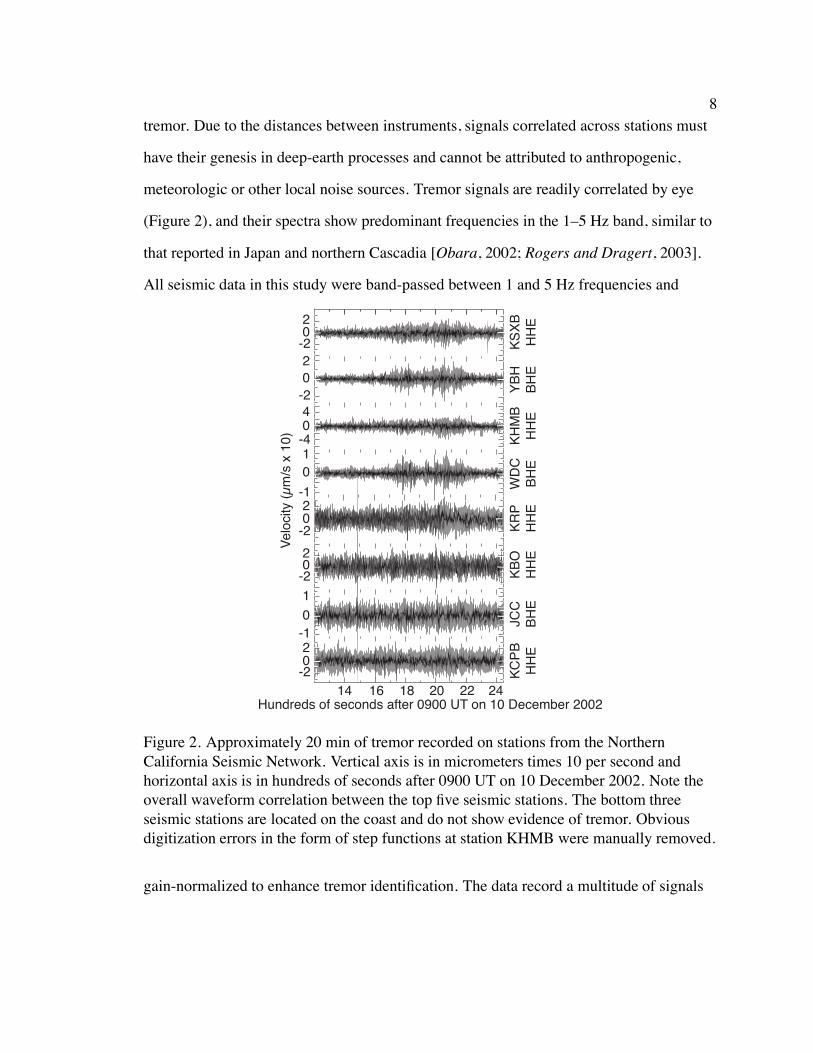
8tremor. Due to the distances between instruments, signals correlated across stations must

have their genesis in deep-earth processes and cannot be attributed to anthropogenic,

meteorologic or other local noise sources. Tremor signals are readily correlated by eye

(Figure 2), and their spectra show predominant frequencies in the 1–5 Hz band, similar to

that reported in Japan and northern Cascadia [Obara, 2002; Rogers and Dragert, 2003].

All seismic data in this study were band-passed between 1 and 5 Hz frequencies and

Hundreds of seconds after 0900 UT on 10 December 2002

-202

-10

1

-202

-202

-1

01

-404

-202

-202

14 16 18 20 22 24

KS

XB

HH

EY

BH

BH

EK

HM

BH

HE

WD

CB

HE

KR

PH

HE

KB

OH

HE

JCC

BH

EK

CP

BH

HE

Vel

ocity

(µm

/s x

10)

Figure 2. Approximately 20 min of tremor recorded on stations from the NorthernCalifornia Seismic Network. Vertical axis is in micrometers times 10 per second andhorizontal axis is in hundreds of seconds after 0900 UT on 10 December 2002. Note theoverall waveform correlation between the top five seismic stations. The bottom threeseismic stations are located on the coast and do not show evidence of tremor. Obviousdigitization errors in the form of step functions at station KHMB were manually removed.

gain-normalized to enhance tremor identification. The data record a multitude of signals

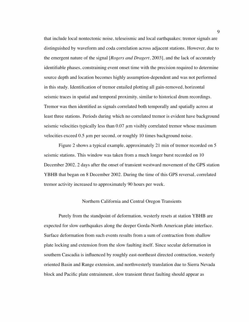
9that include local nontectonic noise, teleseismic and local earthquakes; tremor signals are

distinguished by waveform and coda correlation across adjacent stations. However, due to

the emergent nature of the signal [Rogers and Dragert, 2003], and the lack of accurately

identifiable phases, constraining event onset time with the precision required to determine

source depth and location becomes highly assumption-dependent and was not performed

in this study. Identification of tremor entailed plotting all gain-removed, horizontal

seismic traces in spatial and temporal proximity, similar to historical drum recordings.

Tremor was then identified as signals correlated both temporally and spatially across at

least three stations. Periods during which no correlated tremor is evident have background

seismic velocities typically less than 0.07 µm visibly correlated tremor whose maximum

velocities exceed 0.5 µm per second, or roughly 10 times background noise.

Figure 2 shows a typical example, approximately 21 min of tremor recorded on 5

seismic stations. This window was taken from a much longer burst recorded on 10

December 2002, 2 days after the onset of transient westward movement of the GPS station

YBHB that began on 8 December 2002. During the time of this GPS reversal, correlated

tremor activity increased to approximately 90 hours per week.

Northern California and Central Oregon Transients

Purely from the standpoint of deformation, westerly resets at station YBHB are

expected for slow earthquakes along the deeper Gorda-North American plate interface.

Surface deformation from such events results from a sum of contraction from shallow

plate locking and extension from the slow faulting itself. Since secular deformation in

southern Cascadia is influenced by roughly east-northeast directed contraction, westerly

oriented Basin and Range extension, and northwesterly translation due to Sierra Nevada

block and Pacific plate entrainment, slow transient thrust faulting should appear as

10westerly jumps seen predominantly in the longitude, as is the case. Since it is thought that

slow earthquakes result from fault-fluid migration along the subduction interface, this

lubrication acts to relieve the east-northeast directed contraction caused by subduction of

the Gorda plate, thus the resets seen at station YBHB should be and are opposite to the

direction of subduction. Figure 3, part a shows GPS residuals at station YBHB

demonstrating periodic resets. For comparison, longitude resets from station ALBH, the

time series from which episodic slow Cascadia earthquakes were first identified, are

shown in Figure 3, part c. Residuals from station YBHB in northern California show

similar characteristics as station ALBH, particularly westerly jumps of up to 4.0 mm

occurring at 1997.46, 1998.52, 1999.30, 2000.24, 2001.12, 2001.90, 2002.93 and

2003.81. The amplitudes are similar to those at station ALBH, but the “interseismic”

interval is significantly shorter: 10.9±1.2 months as opposed to 13.9±0.9 months. Forcontrast, time series from nearby stations TRND, CME1, PTSG and MDMT (Figure 1)

show no such resets, indicating the observed resets are not reference-frame artifacts.

Transient slow faulting in northern Cascadia was recognized primarily from deformation

reversals correlated across nearby continuous GPS stations, but the GPS instrument

density in northern California is currently insufficient for any similar correlation. The

nearest continuous GPS station to station YBHB lies on the coast (station PTSG) at a

distance of 120 km; by comparison, there are 7 stations within 60 km of each other in the

northern Puget Basin.

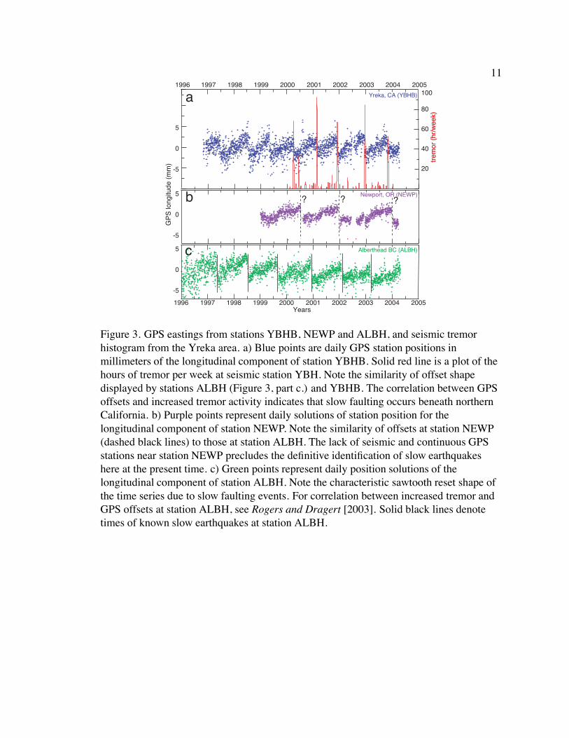
Nonetheless, Figure 3 part a shows the longitude component of station YBHB

overlying a histogram of hours of correlated tremor from nearby seismic station (station

YBH). The remarkable correlation between tremor rate and GPS deformation reversals is

readily apparent and confirms that slow earthquakes occur beneath northern California.

Although background tremor here is detected during many weeks of the year when no

11

1996 1997 1998 1999 2000 2001 2002 2003 2004 2005

-5

0

5

20

40

60

80

100

trem

or (

hr/w

eek)

trem

or (

hr/w

eek)

-5

0

5

GP

S lo

ngitu

de (

mm

)

Yreka, CA (YBHB)

Alberthead BC (ALBH)

1996 1997 1998 1999 2000 2001 2002 2003 2004 2005

-5

0

5 Newport, OR (NEWP)

a

b

c

?? ?

Years

Figure 3. GPS eastings from stations YBHB, NEWP and ALBH, and seismic tremorhistogram from the Yreka area. a) Blue points are daily GPS station positions inmillimeters of the longitudinal component of station YBHB. Solid red line is a plot of thehours of tremor per week at seismic station YBH. Note the similarity of offset shapedisplayed by stations ALBH (Figure 3, part c.) and YBHB. The correlation between GPSoffsets and increased tremor activity indicates that slow faulting occurs beneath northernCalifornia. b) Purple points represent daily solutions of station position for thelongitudinal component of station NEWP. Note the similarity of offsets at station NEWP(dashed black lines) to those at station ALBH. The lack of seismic and continuous GPSstations near station NEWP precludes the definitive identification of slow earthquakeshere at the present time. c) Green points represent daily position solutions of thelongitudinal component of station ALBH. Note the characteristic sawtooth reset shape ofthe time series due to slow faulting events. For correlation between increased tremor andGPS offsets at station ALBH, see Rogers and Dragert [2003]. Solid black lines denotetimes of known slow earthquakes at station ALBH.

12GPS reversals are evident, the rate of tremor increases by an order of magnitude during

GPS reversals. Coastal Oregon also shows preliminary evidence of westerly resets at

station NEWP, located in Newport, Oregon. These reversals have similar amplitudes to

those at station YBHB and northern Puget Basin stations, but do not yet show periodic

behavior. Station NEWP shows three resets in longitude at 2000.52, 2001.98 and 2003.99.

These offsets are not observed at the GPS station CORV, located 60 km inland in

Corvallis, Oregon. The absence of offsets at station CORV is consistent with relatively

narrow, offshore locked and transition zones at this latitude, also suggested from vertical

deformation rates [Mitchell et al., 1994]. Thus, station CORV may lie well east of the

downdip edge of the transition zone where slow earthquakes occur. At the present time,

however, the dearth of GPS or seismic data close to station NEWP precludes

determination of spatially coherent events.

Discussion

The northern California data demonstrate that slow Cascadia earthquakes are not

confined to the structural bight in the Juan de Fuca plate beneath the northern Puget Basin,

and argue that they occur throughout Cascadia and many other subduction zones. More

importantly, these results follow Obara [2002] and Rogers and Dragert [2003] in linking

seismic tremor and slow faulting to one underlying cause, most likely fault-fluid transport

[Melbourne and Webb, 2003]. Analysis of tremor alone for source processes that might

constrain such transport is complex, since the lack of discernible phases prohibits

discrimination between path and source contributions to tremor coda. For example,

delta-function sources, propagated through complex crustal media, have been shown to

cause harmonic volcano tremor originally attributed to resonance at the source [Chouet

et al., 1987; Kedar et al., 1998; Koyanagi et al., 1987]. Moreover, if Cascadia tremor does

13indeed result from a harmonic source at depth, a host of distinct driving mechanisms

could produce source resonance and identical surface observations, again obfuscating the

underlying physics [Chouet et al., 1987; Koyanagi et al., 1987]. If both tremor and slow

slip are manifestations of hydraulic transport resonating and unclamping fault walls that

sandwich pore fluids, an important next step will be to implement experiments that can

constrain near-field (static), non-double couple components of moment release. These, in

turn, will likely be of great use in constraining slow earthquake physics at a resolution

higher than that afforded by either GPS or tremor.

CHAPTER III

EXTENT AND DURATION OF THE 2003 CASCADIA SLOW EARTHQUAKE

Inversion of continuous GPS measurements from the Pacific Northwest show the

2003 Cascadia slow earthquake to be among the largest of 10 transients recognized here.

Twelve stations bracketing slow slip indicate transient slip propagated bidirectionally

from initiation in the southern Puget Basin, reaching 300 km along-strike over a period of

7 weeks. This event produced, for the first time, resolvable vertical subsidence, and

horizontal displacement reaching 6.0 mm in southern Washington State. Inverted for

nonnegative thrust slip, a maximum of 3.8 cm of slip is inferred, centered at 28-km depth

near the sharp arch in the subducting Juan de Fuca plate. Nearly all slip lies shallower

than 38 km. Inverted slip shows a total moment release ofMw = 6.6 and a high degree of

spatial localization rather than near-uniform slip. This suggests rupture concentrated

along asperities holds for slow earthquakes as well as conventional events.

Transient creep events in subduction zones, also known as slow or silent

earthquakes, or episodic tremor and slip events, often occur periodically with recurrence

intervals that range from months to years [Beavan et al., 1983; Kawasaki et al., 1995;

Larson et al., 2004; Linde et al., 1996; Lowry et al., 2001; Ozawa et al., 2001; Sagiya,

2004; Sagiya and Ozawa, 2002]. In Cascadia, 10 slow events have been detected with a

13.9±0.9-month recurrence near the U.S.-Canadian border and six events with a10.9±1.2-month periodicity beneath northern California [Szeliga et al., 2004]. They areobserved with GPS as spatially coherent reversals from secular forearc contraction to

transient extension, and more recently with seismic tremor [Obara, 2002; Rogers and

Dragert, 2003; Szeliga et al., 2004]. However, locating tremor hypocenters remains

14

15challenging due both to the lack of identifiable phases and because its high frequency

content (1–5 Hz) renders it sensitive to small-scale crustal structures, thus resulting in

hypocenters whose accuracy is difficult to assess. The triggers of transient creep thus

remain unknown, but have been hypothesized to stem from pore fluid migration producing

conduit resonance simultaneous with reducing fault-normal stress [Julian, 2002;

Melbourne and Webb, 2003]. Besides a remarkable periodicity, Cascadia creep events also

show characteristic maximum offsets of typically 5 to 8 mm. Whether this is a result of

characteristic slip along specific asperities or is instead a purely elastic masking of

adjacent rupture patches in subsequent events is an important mechanical constraint still

undetermined. Here I invert GPS measurements that constrain slip during the 2003

Cascadia event. The results suggest that slow earthquakes, like conventional ones, have

slip that is coarsely distributed along relatively localized asperities.

Data

Continuous GPS data from the Pacific Northwest Geodetic Array [Miller et al.,

2001] and Western Canada Deformation Arrays [Dragert and Hyndman, 1995] (Figure 4)

was processed with the Gipsy-Oasis II [Lichten and Border, 1987] software utilizing

satellite orbit and clock parameters provided by the Jet Propulsion Laboratory [Heflin

et al., 1992]. Point positioning and precise orbits and clocks were used to analyze the

phase data with ambiguity resolution applied [Zumberge et al., 1997]. Daily positions and

covariance matrices were determined within the ITRF2000 reference frame [Altamimi

et al., 2002] using daily frame products also from the Jet Propulsion Laboratory. A

regional stabilization was applied to each daily position using a reference set of 42

stations from the North America plate region with 23 stations concentrated in the Pacific

Northwest. Of these 42 stations, 33 stations have published positions and velocities in

16

ALBH

CHWK

CHZZ

CPXF

FTS1

GOBSGWEN

JRO1KELS

LIND

LKCP

NANO

NEAH

PABH

PUPU

SATS SC00

SC02 SEDR

TWHL

UCLU

YAWA

RPT1

5 mm/yr5 mm

48ºN

46ºN

50ºN

120ºW124ºW126ºW

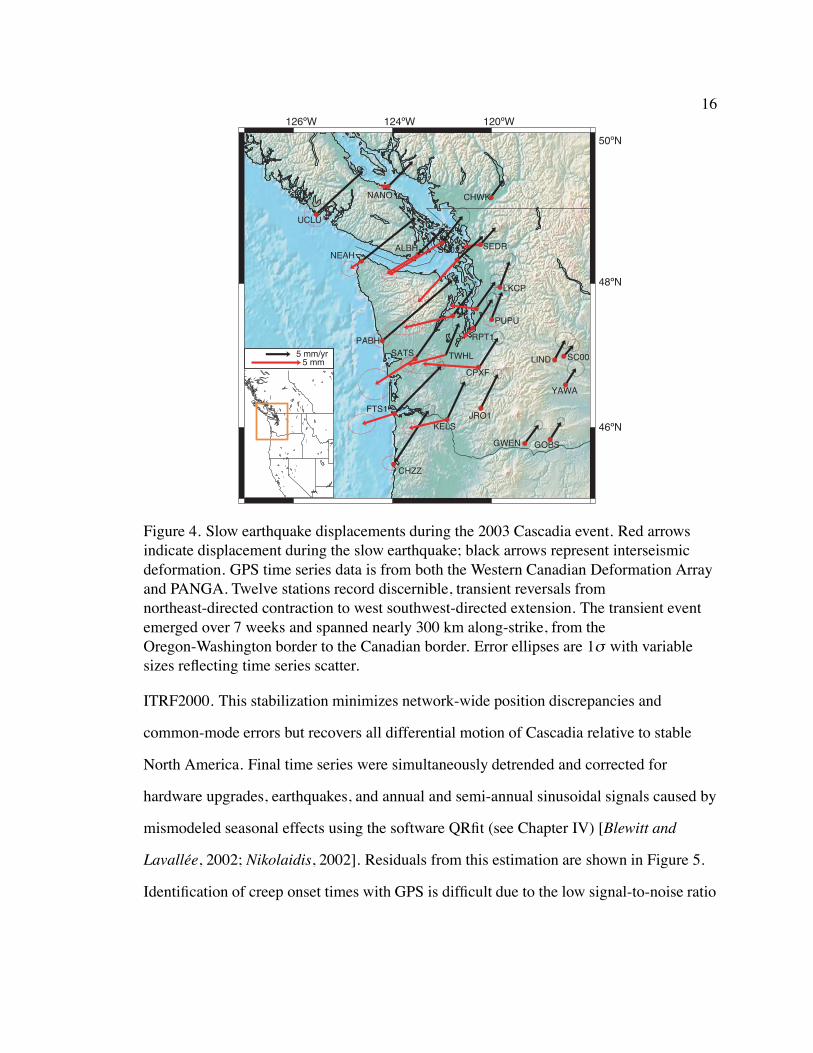
Figure 4. Slow earthquake displacements during the 2003 Cascadia event. Red arrowsindicate displacement during the slow earthquake; black arrows represent interseismicdeformation. GPS time series data is from both the Western Canadian Deformation Arrayand PANGA. Twelve stations record discernible, transient reversals fromnortheast-directed contraction to west southwest-directed extension. The transient eventemerged over 7 weeks and spanned nearly 300 km along-strike, from theOregon-Washington border to the Canadian border. Error ellipses are 1σ with variablesizes reflecting time series scatter.

ITRF2000. This stabilization minimizes network-wide position discrepancies and

common-mode errors but recovers all differential motion of Cascadia relative to stable

North America. Final time series were simultaneously detrended and corrected for

hardware upgrades, earthquakes, and annual and semi-annual sinusoidal signals caused by

mismodeled seasonal effects using the software QRfit (see Chapter IV) [Blewitt and

Lavallee, 2002; Nikolaidis, 2002]. Residuals from this estimation are shown in Figure 5.

Identification of creep onset times with GPS is difficult due to the low signal-to-noise ratio

17

103050

SC02 VERTICAL

0

10

20

30

40

50

60

70

80

90

100

110

120

2000 2001 2002 2003 2004

ALBH

NEAH

SC02

SEDR

WHD1

SEAT

KTBW

RPT1

TWHL

CPXF

FTS1

KELS

??

mm30

GP

S L

ongi

tude

(m

m)

Years

Figure 5. Daily longitude positions record the last three episodic slow earthquakes inCascadia. Unlike previous events, the 2003 event ruptured as far south as the Oregonborder. Station TWHL has irrecoverable data outages at the onset of the event and cannotbe used to constrain onset timing at that station. Station SC02 records the first discerniblevertical subsidence for slow earthquakes, 5±2 mm during this event (note change ofscale). Stations FTS1, PRT1 and WHD1 are U.S. Coast Guard stations with olderantennas mounted on 10-meter towers and have higher intrinsic scatter. (Top) Example ofGaussian wavelet transform used to pick transient onset times (shown is east componentof ALBH, the topmost time series). The y-axis is wavelet scale (temporal extent), x-axis istime, and color denotes relative wavelet coefficient amplitude, with red showing highestamplitudes and blue lowest. Discrete fault slip events produce step-like offsets in thegeodetic time series that propogate across all wavelet scales. This provides a basis forautomated transient detection and correlation with large geodetic station arrays usingwavelets.

18of the measurements. As an alternate to manual event picking, I use the Gaussian wavelet

transform to better identify initiation of rupture. This approach employs the fact that

succeeding wavelet basis functions are increasingly sensitive to temporal localization of

any given signal, unlike the periodic sinusoids of the Fourier transform. Slow faulting at

depth, which effectively produces a Heaviside step at the onset of faulting, appears in the

wavelet transform as an amplitude spike that pervades the wavelet power spectrum

(Figure 5). Faulting initiation is precisely identified from the temporal location of this

spike in amplitudes of wavelet coefficients with greatest localization. Besides being

repeatable and less prone to human or reference-frame biases, the wavelet transform also

allows clear discrimination of slow faulting deformation from other transient, nonsolid

earth signals such as those that arise from colored noise [Langbein and Johnson, 1997].

Furthermore, times picked from the wavelet transform produce a significant reduction in

chi-square misfits in event-offset parameter estimation, at least for short duration

transients lasting less several weeks. Finally, this technique is appealing in that it forms

the basis for automated transient detection in large geodetic networks, such as the Plate

Boundary Observatory, where manual picking of nearly 4000 data channels will not be

feasible.

The 2003 Cascadia Slow Earthquake

Total offsets for the 2003 event (Figures 4 and 5) are sensible in that they suggest a

spatially localized but temporally staggered pattern of simultaneous, north-south

bidirectional propagation of reversals from contraction to transient extension throughout,

but limited to, the northern Cascadia forearc. The first significant departure from secular

contraction is recorded simultaneously beneath the southern Puget Basin in late January

2003 on stations SEAT, KTBW, and RPT1 (Figures 4 and 5). Within a time span of less

19than 1 month, transient reversals then appear simultaneously to the north (stations SEDR

and WHD1). By mid-February, 2003, about 3 weeks after its initiation, creep had spread

200 km north and south, reaching southwestern British Columbia (stations SCO2, NEAH,

ALBH) and southernmost Washington (stations CPXF, KELS, FTS1, JR01). By March

2003, 6 weeks after nucleation, the transient is evident on 12 stations. Although its

termination is difficult to precisely identify, the data suggest that by mid-March slow slip

had terminated along the entire margin. Displacements as great as 6±1 mm are recoveredin the southern Puget Basin (station CPXF), resolvable extension reaches as far south as

the Oregon border, and vertical subsidence of 5±2 mm is visible in the northern PugetBasin (station SC02).

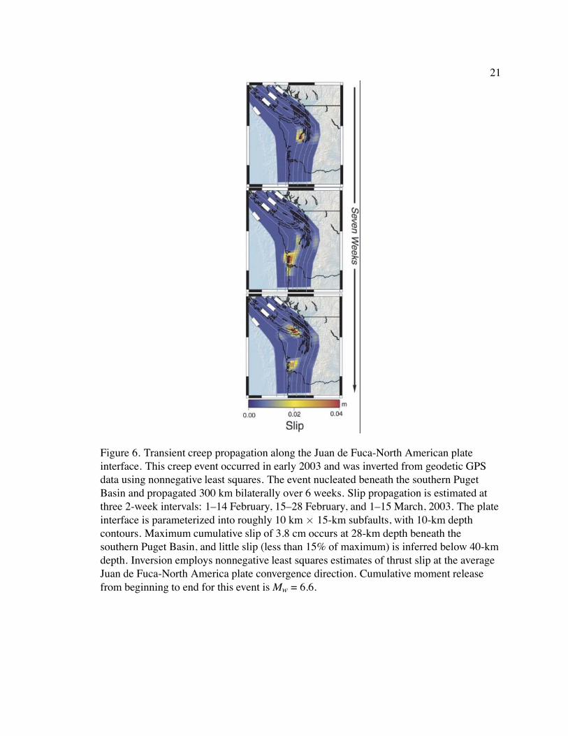
The density of stations on which the 2003 slow event was recorded invites a

formal inversion of the surface displacement field for a variable-slip distribution along the

plate interface. I discretized the Juan de Fuca-North American plate interface [Fluck

et al., 2000] into 10 km × 25 km subfaults along the downdip and along-strikecomponents, respectively. The plate interface intersects the Earth’s surface at the

geomorphic expression of the offshore deformation front and extends to an absolute depth

of 70 km, far below the region of expected faulting. Green’s functions for both an elastic

half-space and layer-cake were computed using the methodologies of Okada [1992] and

Zhu and Rivera [2002] and were found not to differ significantly for deep (greater than 10

km) sources. A Laplacian smoothing operator is incorporated into the design matrix,

following Harris and Segall [1987]. The Laplacian smoothing operator serves to

constrain the moment of the inversion while preventing grossly disconnected slip

distributions. An optimal smoothing coefficient was derived using a cross-validation

method in which single stations were sequentially removed and the remaining data

compared with the surface displacements predicted by inversion based on the incomplete

20data set (see Chapter V). This procedure is then repeated for each station and for multiple

smoothing parameter values. The smoothing parameter, which minimized misfit, was then

adopted for the inversions shown in Figure 6. The design matrix was inverted with QR

decomposition constrained to solve only for positive thrust slip [Lawson and Hanson,

1995]. Offsets from cleaned time series estimated biweekly were inverted for cumulative

slip during that time period. Figure 6 shows three biweekly time slices starting in early

February and continuing through mid-March 2003. Transient faulting clearly nucleated

below the southern Puget Basin, propagated along-strike bidiagonally from this region,

reached maximum slip by mid-March of 2003, and faded in the south prior to the north. A

maximum of 3.8 cm of cumulative slip is imaged beneath the southern Puget Basin.

Discussion

Moment release, which I estimate by summing inverted slip over time, is largely

invariant with respect to the details of the slip distribution so long as the inverted slip

produces vectors that match the data. The cumulative moment release of this event isMw =

6.6. Among the largest of the Cascadia events (perhaps due to instrumentation), this event

is still significantly smaller than other slow events reported elsewhere, for instance in

western Mexico (Mw = 7.5) [Lowry et al., 2001]. The slip heterogeneity shown in Figure 6

is likely real, since inversions based on a coarser parameterization of the plate interface

fail to fit the data adequately. Moreover, inversion of synthetic time series with the

relatively fine subfaults shown in Figure 6 suggests that evenly distributed, wide-spread

creep spread over hundreds of kilometers, instead of patchy slip localized over several

tens of kilometers, should be resolved by the 12 stations. Beyond these dimensions, the

inversions cannot reveal details of slip, which effectively precludes estimating stress drop

from surface deformation measurements alone. Tremor studies of slow earthquakes, by

21

Figure 6. Transient creep propagation along the Juan de Fuca-North American plateinterface. This creep event occurred in early 2003 and was inverted from geodetic GPSdata using nonnegative least squares. The event nucleated beneath the southern PugetBasin and propagated 300 km bilaterally over 6 weeks. Slip propagation is estimated atthree 2-week intervals: 1–14 February, 15–28 February, and 1–15 March, 2003. The plateinterface is parameterized into roughly 10 km × 15-km subfaults, with 10-km depthcontours. Maximum cumulative slip of 3.8 cm occurs at 28-km depth beneath thesouthern Puget Basin, and little slip (less than 15% of maximum) is inferred below 40-kmdepth. Inversion employs nonnegative least squares estimates of thrust slip at the averageJuan de Fuca-North America plate convergence direction. Cumulative moment releasefrom beginning to end for this event isMw = 6.6.

22contrast, consistently indicate that the deformation observed at the surface likely reflect

the summation of elastic strain from a large number of tiny faulting events clustered in

time [Kao and Shan, 2004; Rogers and Dragert, 2003; Szeliga et al., 2004].

The stress drop of these tiny events will likely constrain the rupture mechanism of

slow earthquakes. As a result, source constraints on these smaller events deduced from

tremor seismicity will likely prove most fruitful in determining how rupture fronts

propagate along the plate interface. Broadband recordings that might document

dilatational components of faulting would prove particularly valuable in understanding

these new phenomena.

CHAPTER IV

QRFIT, A FLEXIBLE UTILITY FOR TIME SERIES DECOMPOSITION

In the last decade, solid earth researchers have benefited from a remarkable

increase in the signal-to-noise ratio of geodetic time series. This increase in positioning

capability to sub-centimeter resolution has allowed new signals from a variety of solid

earth processes to be detected. Among these include periodic fault creep events [Miller

et al., 2002], multi-year transients following large earthquakes [Cohen and Freymueller,

1997;Melbourne et al., 2002], and variations in strain accumulation rate along hazardous

faults [Gao et al., 2000]. However, measurements from continuously operating GPS

stations in particular display numerous signals from known nonsolid earth sources, and

the ability to detect new tectonic processes from these measurements is wholly dependent

on removing these known signals. Linear station velocities, annual and semi-annual

signals from a multitude of sources [Blewitt et al., 2001; Kedar et al., 2003], and discrete

offsets due to site maintenance are just a few of the signals with known origin that may be

estimated. Other signals, such as slow earthquakes and postseismic crustal relaxation,

may also be recognized and removed, even if their parameterization is empirical rather

than derived from a complete understanding of the underlying processes. In many cases,

transient solid earth signals only become recognizable after removal of known signals.

Here I present a generalizable method of geodetic time series decomposition with

accompanying software that is both easily modified and portable. I begin by describing

the formal estimation procedure for known signals in GPS time series. This procedure is

then applied to GPS time series from 145 IGS stations. The software developed for signal

estimation is available under the GNU General Public License.

23

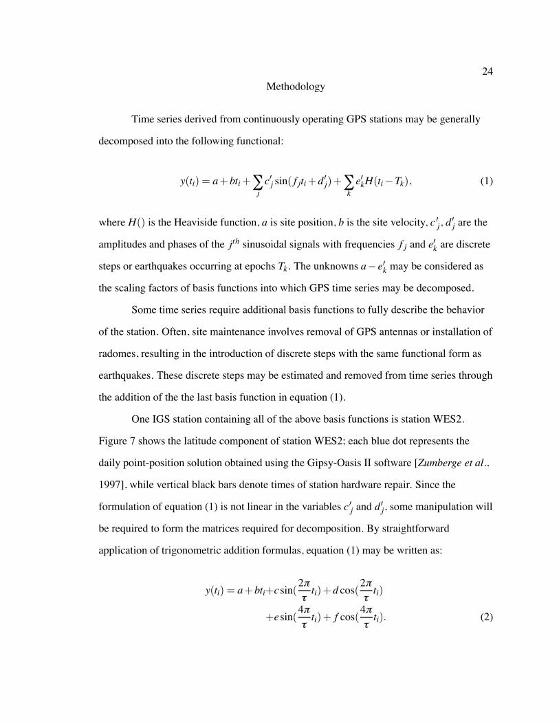
24Methodology

Time series derived from continuously operating GPS stations may be generally

decomposed into the following functional:

y(ti) = a+bti+∑jc′j sin( f jti+d′j)+∑

k

e′kH(ti−Tk), (1)

where H() is the Heaviside function, a is site position, b is the site velocity, c ′j, d′j are the

amplitudes and phases of the jth sinusoidal signals with frequencies f j and e′k are discrete

steps or earthquakes occurring at epochs Tk. The unknowns a− e′k may be considered as

the scaling factors of basis functions into which GPS time series may be decomposed.

Some time series require additional basis functions to fully describe the behavior

of the station. Often, site maintenance involves removal of GPS antennas or installation of

radomes, resulting in the introduction of discrete steps with the same functional form as

earthquakes. These discrete steps may be estimated and removed from time series through

the addition of the the last basis function in equation (1).

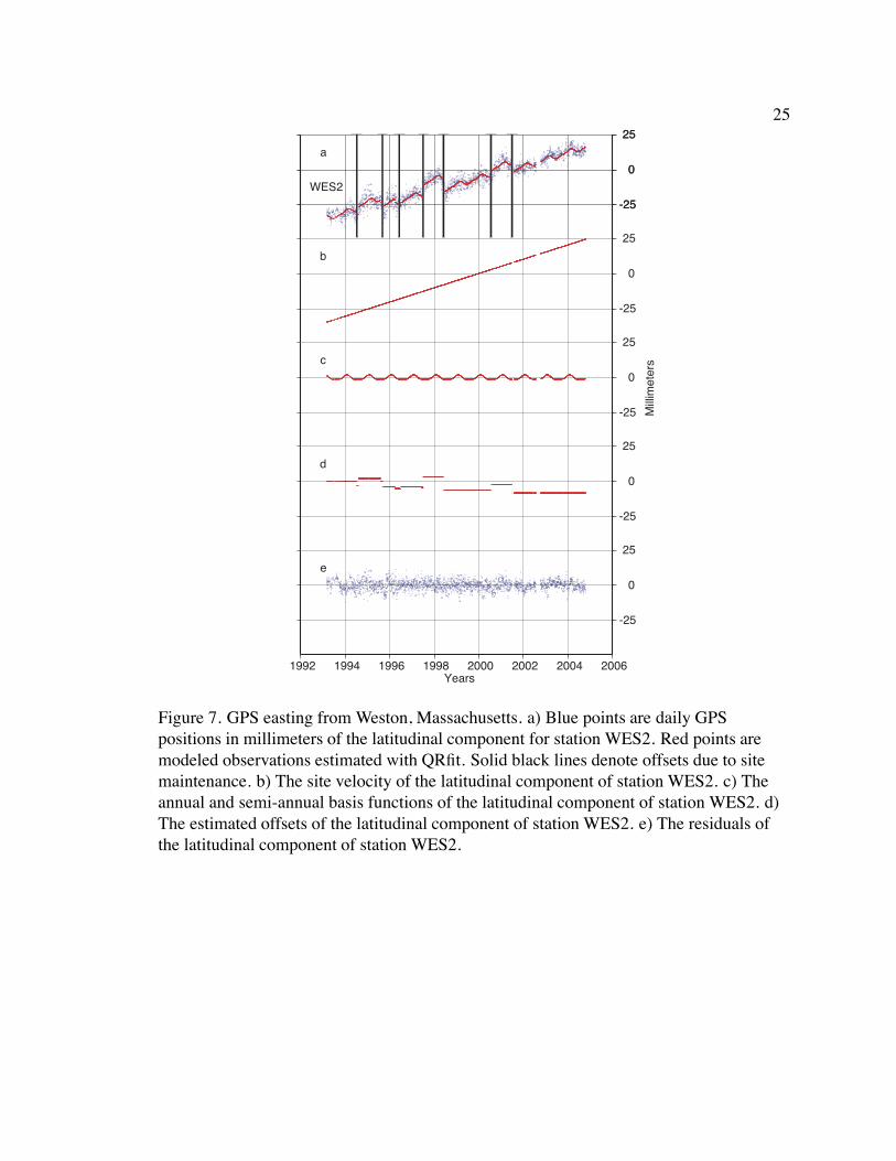
One IGS station containing all of the above basis functions is station WES2.

Figure 7 shows the latitude component of station WES2; each blue dot represents the

daily point-position solution obtained using the Gipsy-Oasis II software [Zumberge et al.,

1997], while vertical black bars denote times of station hardware repair. Since the

formulation of equation (1) is not linear in the variables c′j and d′j, some manipulation will

be required to form the matrices required for decomposition. By straightforward

application of trigonometric addition formulas, equation (1) may be written as:

y(ti) = a+bti+csin(2πτti)+d cos(

2πτti)

+esin(4πτti)+ f cos(

4πτti). (2)

25

-25

0

25

-25

0

25

WES2

a

-25

0

25

b

-25

0

25

c

-25

0

25

d

-25

0

25

1992 1994 1996 1998 2000 2002 2004 2006

e

Mill

imet

ers

Years

Figure 7. GPS easting from Weston, Massachusetts. a) Blue points are daily GPSpositions in millimeters of the latitudinal component for station WES2. Red points aremodeled observations estimated with QRfit. Solid black lines denote offsets due to sitemaintenance. b) The site velocity of the latitudinal component of station WES2. c) Theannual and semi-annual basis functions of the latitudinal component of station WES2. d)The estimated offsets of the latitudinal component of station WES2. e) The residuals ofthe latitudinal component of station WES2.

26Here a and b are as in equation (1) while combinations of c and d describe an annual

signal, e and f describe a semi-annual signal and τ is the period. Since equation (2) is

linear in the unknowns a− f , one may form the matrix:

A=

⎛⎜⎜⎜⎜⎝1 t0 sin(2πτ t0) cos(2πτ t0) sin(4πτ t0) cos(4πτ t0)......

......

......

1 tn sin(2πτ tn) cos(2πτ tn) sin(4πτ tn) cos(4πτ tn)

⎞⎟⎟⎟⎟⎠ , (3)

where n is the number of GPS position observations. Equation (2) may now be rewritten

in matrix-vector form as:

y= Ax+ r, (4)

where x is a vector consisting of the unknowns a− f , y is a vector consisting of GPS

position observations, and r is a vector of residuals.

Solution of the system of equations (equation (4)) proceeds by forming the

weighted normal equations with weight matrixC consisting of the inverse covariances of

the observations y:

AtCAx= AtCy, (5)

where At denotes the matrix transpose of A. Following Nikolaidis [2002], one may

achieve the best linear unbiased estimate of the vector x by using the QR decomposition

of equation (5). Equation (5) then becomes:

x= R−1QtAtCy,

where Q is an orthogonal matrix, R is a right-triangular matrix, and QR= AtCA.

Computationally, QR decomposition is more numerically stable than explicitly inverting

the weighted normal equations (equation (5)).

27By defining the residual time series as r = y−Ax, one may then propagate

covariances forward to yield covariances (Σ) for the unknowns, modeled observations,

and residuals:

σ20 =rtCrn−m

, (6)

Σx =σ20 (AtCA)−1,

ΣAx =σ20A(AtCA)−1At ,

Σr =σ20 (C−1−A(AtCA)−1At).

In equation (6), m is the number of basis functions used in the decomposition and n is the

number of observations.

QRfit

Following the theory outlined in the previous section, I have written the program

QRfit. This software was originally designed to aid in the automated analysis of GPS time

series from the PANGA network.

Implementation

QRfit is written in C for maximum portability and utilizes functions from the GNU

Scientific Library [Galassi et al., 2003]. The inclusion of the GNU Scientific Library in

QRfit requires that my code distribution must also be under the GNU General Public

License. Further, the GNU General Public License requires that all improved versions of

QRfit be free software. For a more complete explanation of the philosophy of the GNU

General Public License see http://www.gnu.org/philosophy.

28Care has been taken to allow QRfit to be compiled on a variety of computer

architectures by utilizing the GNU Autotools programs Autoconf and Automake.

Additionally, QRfit is provided with a UNIX-style manual page explaining the details of

program execution, input, and output formats.

Code for individual functions in QRfit has been modularized in an attempt to make

the program more readable to researchers and therefore easier to maintain. The

modularization of the source code enables the user to alter the basis functions into which

the time series is decomposed. This modularization presents researchers in other fields

with the opportunity to alter QRfit to decompose time series into their own basis functions.

To decompose a time series into an alternate set of basis functions, the basis functions

must be linearizable in terms of the unknowns following the previous section. If the basis

functions are linearizable, the columns of the design matrix in equation (4) would then

consist of the partial derivatives of each basis function in terms of its unknowns.

Decomposition of equation (5) is performed using functions from the GNU

Scientific Library which implement the Householder QR algorithm of Golub and Van

Loan (Algorithm 5.2.1 in Golub and Val Loan [1996]). This method is more numerically

stable than explicitly inverting AtCA. The output from QRfit is chosen by the user at

run-time, and may consist of merely the parameters solved for, the residual of the time

series minus the modeled observations, or the modeled time series observations.

Input consists of a three-column ASCII file with columns of observation time,

position, and uncertainty. Due to the inherent dimensions involved in forming and solving

equation (5), decomposing an 8200 data point time series into linear, annual, and

semi-annual components will require approximately 1 gigabyte of memory. If each datum

represents 1 day of GPS data, 8200 data points represents more than 22 years of GPS data.

29Output follows the same pattern with the uncertainty corresponding to the

appropriate formula from equation (6). Outlier deweighting may be implemented with the

user defining the number of standard deviations a point must be for it to be heavily

deweighted. Points deemed by QRfit to be greater than the user-defined number of

standard deviations are then output to a user-defined file. Hardware offsets are specified in

a one-column ASCII file consisting of times for each known offset.

Application of QRfit to IGS Data

I have used QRfit to estimate the annual and semi-annual signals and phases at

certain IGS stations. Some IGS stations have not been included either because of some

pathological problem with the station has hindered estimation, or the station had not been

observing long enough to properly estimate annual and semi-annual signals. I find annual

signal variations of up to 10.02 mm with a mean amplitude of 2.22 mm and semi-annual

variations up to 7.76 mm with a mean of 1.02 mm.

Summary

The consequences of ignoring annual and semi-annual signals during parameter

estimation of GPS time series can be significant [Blewitt and Lavallee, 2002]. I have

produced a program to decompose GPS time series into meaningful geophysical basis

functions by simultaneously estimating various parameters including annual and

semi-annual signals. This program utilizes the technique of QR decomposition to solve

the normal equations in a least squares sense. I have applied my program by estimating

annual and semi-annual signals in 145 IGS stations. Although the focus of this chapter is

on GPS time series, the modularization of our available computer code allows for the

analysis of other geophysical time series such as oceanic tide gauges and tiltmeters.

CHAPTER V

GPS INVERSION WITH POSITIVITY CONSTRAINTS

Continuous observations using GPS have revealed periodic slow or silent

earthquakes along the Cascadia subduction zone with a spectrum of timing and

periodicity. These creep events perturb time series of GPS observations and yield coherent

displacement fields that relate to the extent and magnitude of fault displacement. The

inversions employed in this study utilize Okada’s elastic dislocation model and a

nonnegative least squares approach [Lawson and Hanson, 1995; Okada, 1992].

Methodologies for optimizing the slip distribution smoothing parameter for a particular

station distribution are investigated to significantly reduce the number of possible slip

distributions and the range of estimates for total moment release for each event. The

discritized slip distributions calculated from multiple creep events identify areas of the

Cascadia plate interface where slip persistently recurs. The current hypothesis, that slow

earthquakes are modulated by forced fluid flow, leads to the possibility that some regions

of the Cascadia plate interface may display fault patches preferentially exploited by fluid

flow. Thus, the identification of regions of the plate interface that repeatedly slip during

slow events may yield important information regarding the identification of these fluid

pathways.

Inversion of a GPS vector displacement field often requires additional assumptions

in order to reduce instability and nonuniqueness of the solution. In the following, I present

methodologies for reducing nonuniqueness and enhancing stability in GPS vector field

inversion. This stabilization is achieved through the addition of a priori information

during the inversion process. One may formulate the GPS displacement inversion problem

30

31by assuming that deformation observed at the Earth’s surface is related to fault

displacement at depth plus random error. Then the problem of inverting a surface

displacement vector d for slip at depth s is reduced to solving the matrix equation

Gs= d, (7)

where G is a Jacobian matrix of Green’s functions relating surface displacement to fault

slip. Often, this matrix equation is severely underdetermined (i.e., if G is an (M×N)

matrix, thenM� N). In the underdetermined case, additional a priori information is

required to reduce nonuniqueness and aid in stabilizing the inversion process.

Two constraints that are often utilized to help stabilize the solution of equation (7),

are positivity and solution smoothness. The first constraint, positivity, is achieved through

the nonnegative least squares algorithm of Lawson and Hanson [1995]. The second

constraint, smoothing, is often accomplished by augmenting the matrix G with additional

rows which encode a finite difference approximation of the Laplacian operator and

augmenting the observation vector d with an equal number of rows containing zeros.

While the augmentation of the original problem with these two constraints does not

entirely eliminate the problem of nonuniqueness, it does reduce the number of possible

slip distributions.

With the introduction of the smoothing constraint, one also requires a smoothing

parameter to control the degree of smoothing present in the solution. The addition of this

smoothing parameter introduces the problem of optimal smoothing parameter selection. I

present a methodology for smoothing parameter selection using the technique of cross

validation. Often the method of cross validation is avoided due to its high computational

cost. Through the application of a computer message passing system, I am able to

parallelize computation and reduce the time required for smoothing parameter selection

by a factor of O(1/n) where n is the number of processors used.

32Nonnegative Least Squares

The constraint that the solution vector s in equation (7) contain only nonnegative

coordinates falls under the general category of linear least squares with linear inequality

constraints. The problem of nonnegative least squares may be formally cast as:

Minimize ‖Gs−d‖ subject to s≥ 0. (8)

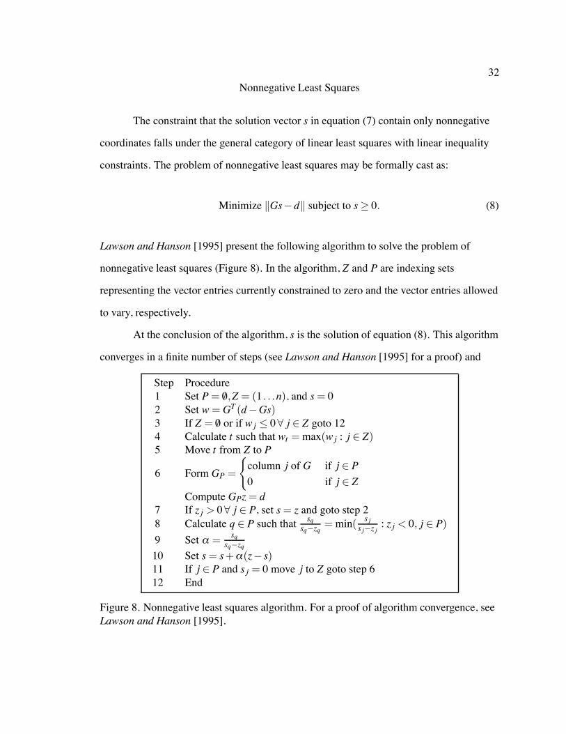
Lawson and Hanson [1995] present the following algorithm to solve the problem of

nonnegative least squares (Figure 8). In the algorithm, Z and P are indexing sets

representing the vector entries currently constrained to zero and the vector entries allowed

to vary, respectively.

At the conclusion of the algorithm, s is the solution of equation (8). This algorithm

converges in a finite number of steps (see Lawson and Hanson [1995] for a proof) and

Step Procedure1 Set P= /0,Z = (1 . . .n), and s= 02 Set w=GT (d−Gs)3 If Z = /0 or if wj ≤ 0∀ j ∈ Z goto 124 Calculate t such that wt =max(wj : j ∈ Z)5 Move t from Z to P

6 Form GP =

{column j of G if j ∈ P0 if j ∈ Z

Compute GPz= d7 If z j > 0∀ j ∈ P, set s= z and goto step 28 Calculate q ∈ P such that sq

sq−zq =min( s js j−z j : z j < 0, j ∈ P)

9 Set α = sqsq−zq

10 Set s= s+α(z− s)11 If j ∈ P and s j = 0 move j to Z goto step 612 End

Figure 8. Nonnegative least squares algorithm. For a proof of algorithm convergence, seeLawson and Hanson [1995].

33requires no explicit parameter selection by the user. Due to the complexity in the

construction of the solution vector however, an explicit formula for formal covariance

propagation has not been found. Thus while the algorithm may be used in a “black box”

manner, an accurate assessment of the covariances on the solution requires more

complicated computation.

Smoothing and Cross Validation

While the requirement that the solution vector s be nonnegative requires no

parameter selection by the user, the constraint that the solution be spatially smooth does

require the estimation of an optimal smoothing parameter. Thus, the problem of finding a

stable solution to equation (7), while incorporating both positivity and smoothing

constraints, is reduced to the problem of optimal parameter selection.

Cross-validation schemes involve repeatedly solving a data-reduced vector form of

Gs= d and constructing a bootstrap estimate of the overall ability of the data set d to

predict missing data subsets [Efron and Tibshirani, 1994]. “Leave-One-Out” cross

validation is one end-member of the cross-validation scheme where the data-reduced

vector is formed by removing one data point at a time. Parameter estimation then

proceeds by solving the data-reduced equation Gs= d, using s to forward predict the

removed data point, and recording the squared misfit between the removed data and its

predicted value. The removed data point is then replaced and a new data point is removed.

For each smoothing parameter value, a sum of squared misfits metric may be calculated,

with the minimum sum of squared misfit providing the optimal parameter.

34Parallel Virtual Machine

The method of cross-validation is utilized for parameter selection in various fields

but is often criticized for being both computationally expensive and time consuming.

Using a data parallel programming methodology, the overall computation time can be

reduced. The Parallel Virtual Machine software library provides routines to distribute

computing tasks amongst numerous networked computers [Geist et al., 1994]. In the

cross-validation algorithm, the calculations associated with each data-reduced vector are

entirely independent. This task independence may be utilized to allow the cross-validation

algorithm to be carried out in parallel, distributed across multiple machines. Figure 9

displays an algorithm for the parallel distribution and computation of a cross-validation

scheme for the determination of an optimal smoothing parameter. With the use of the

Parallel Virtual Machine software library, computation time for optimal smoothing

parameter selection with cross validation is reduced by O(1/n), where n is the number of

processors used in the calculation. In reality, however, there exists a lower limit to the

computation time achievable. Beyond this limit, the addition of more processors no longer

decreases computation time as the overhead of network communication becomes a

limiting factor.

Application

Calculation of the optimal smoothing parameters used to invert surface

displacements for the 2003 slow earthquake was performed using the algorithm outlined

above. The computer message passing environment Parallel Virtual Machine was utilized

with nine 2.9 GHz Intel Pentium 4 CPUs to speed calculation. Parallel Virtual Machine

was chosen over other parallelization environments to perform the calculations since it

does not require homogeneity in the computer systems used. Further, Parallel Virtual

35

Read in array of stations

Initialize smoothing parameter

Enroll process in Parallel Virtual Machine

Spawn slave tasks

Assign one station per task

Invert data using current smoothing parameter with station removed

Predict station deformation for removed station

Calculate residual between prediction and measurement for removed station

Report answer to master process

Calculate sum of squared residuals for each task assigned

Master Process Slave Processes

[Station array][exhausted ]

Increment smoothing parameter

Output file containing CVSS vs. smoothing parameter

[Stations remaining][in array ]

[All requested smoothing][parameters calculated ]

Initialize station array

Figure 9. Unified modeling language representation of the parallel cross-validation sum ofsquares algorithm.

Machine allows for the utilization of large collections of heterogeneous networked

computers to speed calculation of parallel algorithms. Significant speed increases are

observed by utilizing the algorithm outlined above with just nine CPUs. Using nine

processors, a cross-validation sum of squares smoothing parameter estimation for a

real-world problem, the 2003 slow earthquake observed on the PANGA GPS network

demonstrated a processing-time decrease of 89%.

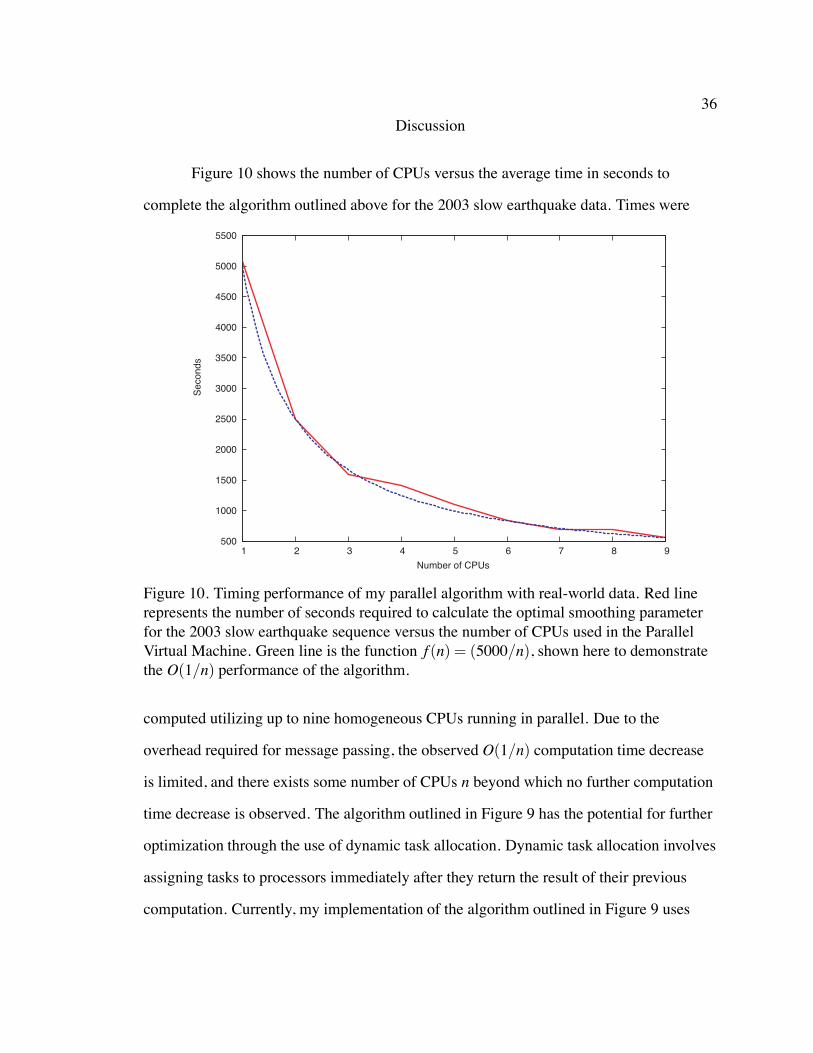
36Discussion

Figure 10 shows the number of CPUs versus the average time in seconds to

complete the algorithm outlined above for the 2003 slow earthquake data. Times were

500

1000

1500

2000

2500

3000

3500

4000

4500

5000

5500

1 2 3 4 5 6 7 8 9

Sec

onds

Number of CPUs

Figure 10. Timing performance of my parallel algorithm with real-world data. Red linerepresents the number of seconds required to calculate the optimal smoothing parameterfor the 2003 slow earthquake sequence versus the number of CPUs used in the ParallelVirtual Machine. Green line is the function f (n) = (5000/n), shown here to demonstratethe O(1/n) performance of the algorithm.

computed utilizing up to nine homogeneous CPUs running in parallel. Due to the

overhead required for message passing, the observed O(1/n) computation time decrease

is limited, and there exists some number of CPUs n beyond which no further computation

time decrease is observed. The algorithm outlined in Figure 9 has the potential for further

optimization through the use of dynamic task allocation. Dynamic task allocation involves

assigning tasks to processors immediately after they return the result of their previous

computation. Currently, my implementation of the algorithm outlined in Figure 9 uses

37static task allocation. Static task allocation involves waiting for all of the calculations

allocated at each step of the algorithm to be completed before new tasks are assigned.

Dynamic task allocation can result in further computation time decreases when the

processors involved in the Parallel Virtual Machine are heterogeneous, since some

processors may be faster than others. Due to the CPU homogeneity in my computer

laboratory, however, performance gains from dynamic task allocation should be minimal.

Conclusion

In this study, I define the optimal smoothing parameter for a given problem as the

minimum of a plot of smoothing parameter versus cross- validation sum of squares score.

The minimum of this function corresponds to the smoothing parameter that best predicts

missing data from the full observation data set. This is a sensible measure since it also

selects an amount of smoothing which minimizes the overall misfit between observations

and predictions while requiring slip to be smoothly varying. While other methodologies

for smoothing parameter selection are available such as generalized cross validation and

L-curve analysis, they are not valid when constrained least squares methods, such as

nonnegative least squares, are utilized [Hansen, 1998]. If constrained least squares

methods are used, brute force methods akin to the algorithm outlined in Figure 9 become

necessary.

REFERENCES

Altamimi, Z., P. Sillard, and C. Boucher (2002), ITRF2000: A new release of the

International Terrestrial Reference Frame for Earth Science applications, J. Geophys.

Res., 107(B10), doi:10.1029/2001JB000561.

Beavan, J., E. Hauksson, S. R. McNutt, R. Bilham, and K. H. Jacob (1983), Tilt and

seismicity changes in the Shumagin seismic gap, Science, 22(4621), 322–325.

Blewitt, G., and D. Lavallee (2002), Effect of annual signals on geodetic velocity, J.

Geophys. Res., 107(B7), doi:10.1029/2001JB000570.

Blewitt, G., D. Lavallee, P. Clarke, and K. Nurutdinov (2001), A new global mode of earth

deformation; seasonal cycle detected, Science, 294, 2342–2345.

Chouet, B., R. Koyanagi, and K. Aki (1987), Origin of volcanic tremor in Hawaii; Part II,

Theory and discussion, in Volcanism in Hawaii, pp. 1259–1280, U. S. Geological

Survey, Reston, Va.

Cohen, S., and J. Freymueller (1997), Deformation of the Kenai Peninsula, J. Geophys.

Res., 102(B9), 20,479–20,487.

Dragert, H., and R. Hyndman (1995), Continuous GPS monitoring of elastic strain in the

northern Cascadia subduction zone, Geophys. Res. Lett., 22, 755–758.

Dragert, H., K. Wang, and T. James (2001), A silent slip event on the deeper Cascadia

subduction interface, Science, 292(5521), 1525–1528.

Efron, B., and R. Tibshirani (1994), An Introduction to the Bootstrap, Chapman and

Hall/CRC, London, UK.

38

39Fluck, P., R. D. Hyndman, and K. Wang (2000), 3-D dislocation model for great

earthquakes of the Cascadia subduction zone, in Penrose conference “Great Cascadia

earthquake tricentennial,” edited by J. J. Clague, B. F. Atwater, K. Wang, Y. Wang, and

I. G. Wong, p. 48, Oregon Department of Geology and Mineral Industries.

Galassi, M., J. Davies, J. Theiler, B. Gough, G. Jungman, M. Booth, and F. Rossi (2003),

GNU Scientific Library Reference Manual, 2nd ed., Network Theory Ltd, Bristol, UK.

Gao, S., P. Silver, and A. Linde (2000), A comprehensive analysis of deformation data at

Parkfield, California; detection of a long-term strain transient, J. Geophys. Res.,

105(B2), 2955–2967.

Geist, A., A. Beguelin, J. Dongarra, W. Jiang, R. Manchek, and V. Sunderam (1994),

PVM: Parallel Virtual Machine. A Users’ Guide and Tutorial for Networked Parallel

Computing, MIT Press, Cambridge, Ma.

Golub, G., and C. Val Loan (1996),Matrix Computations, John Hopkins University Press,

Baltimore, Md.

Hansen, P. C. (1998), Rank-Deficient and Discrete Ill-Posed Problems: Numerical Aspects

of Linear Inversion, Society for Industrial and Applied Mathematics, Philadelphia, Pa.

Harris, R. A., and P. Segall (1987), Detection of a locked zone at depth on the Parkfield,

California, segment of the San Andreas Fault, J. Geophys. Res., 92(8), 7945–7962.

Heflin, M., et al. (1992), Global geodesy using GPS without fiducial sites, Geophys. Res.

Lett., 19(2), 131–134.

Heki, K., S. Miyazaki, and H. Tsuji (1997), Silent fault slip following an interplate thrust

earthquake at the Japan Trench, Nature, 386(6625), 595–598.

40Hirose, H., K. Hirahara, F. Kimata, N. Fujii, and S. Miyazaki (1999), A slow thrust slip

event following the two 1996 Hyuganada earthquakes beneath the Bungo Channel,

southwest Japan, Geophys. Res. Lett., 26(21), 3237–3240.

Julian, B. (2002), Seismological detection of slab metamorphism, Science, 296(5573),

1625–1626.

Kao, H., and S.-J. Shan (2004), The source-scanning algorithm; mapping the distribution

of seismic sources in time and space, Geophys. J. Int., 157, 589–594.

Kawasaki, I., Y. Asai, Y. Tamura, T. Sagiya, N. Mikami, Y. Okada, M. Sakata, and

M. Kasahara (1995), The 1992 Sanriku-Oki, Japan, ultra-slow earthquake, J. Phys.

Earth, 43(2), 105–116.

Kedar, S., H. Kanamori, and B. Sturtevant (1998), Bubble collapse as the source of tremor

at Old Faithful Geyser, J. Geophys. Res., 103(B10), 24,283–24,299.

Kedar, S., G. Hajj, B. Wilson, and M. Heflin (2003), The effect of the second order GPS

ionospheric correction on receiver positions., Geophys. Res. Lett., 30(16),

doi:10.1029/2003GL017639.

Kostoglodov, V., S. Singh, A. Santiago, S. Franco, K. Larson, A. Lowry, and R. Bilham

(2003), A large silent earthquake in the Guerrero seismic gap, Mexico, Geophys. Res.

Lett., 30(15), doi:10.1029/2003GL017219.

Koyanagi, R., B. Chouet, and K. Aki (1987), Origin of volcanic tremor in Hawaii; Part I,

Data from the Hawaiian Volcano Observatory 1969-1985, in Volcanism in Hawaii, pp.

1221–1257, U. S. Geological Survey, Reston, Va.

Langbein, J., and H. Johnson (1997), Correlated errors in geodetic time series;

implications for time-dependent deformation, J. Geophys. Res., 102, 591–604.

41Larson, K., A. Lowry, V. Kostoglodov, W. Hutton, O. Sanchez, K. Hudnut, and G. Suarez

(2004), Crustal deformation measurements in Guerrero, Mexico, J. Geophys. Res., 109,

B04409, doi:10.1029/2003JB002843.

Lawson, C. L., and R. Hanson (1995), Solving Least Squares Problems, Classics in

Applied Mathematics, vol. 15, Soc. for Ind. and Appl. Math., Philadelphia, Pa.

Lichten, S., and J. Border (1987), Strategies for high-precision global positioning system

orbit determination, J. Geophys. Res., 92(B12), 12,751–12,762.

Linde, A., and P. Silver (1989), Elevation changes and the great 1960 Chilean earthquake;

support for aseismic slip, Geophys. Res. Lett., 16(11), 1305–1308.

Linde, A. T., M. T. Gladwin, M. J. S. Johnston, R. L. Gwyther, and R. G. Bilham (1996),

A slow earthquake sequence on the San Andreas Fault, Nature, 383(6595), 65–68.

Lowry, A., K. Larson, V. Kostoglodov, and R. Bilham (2001), Transient fault slip in

Guerrero, southern Mexico, Geophys. Res. Lett., 28(19), 3753–3756.

Melbourne, T., and F. Webb (2002), Preseismic transient slip during the 2001Mw = 8.4

Peru earthquake sequence from continuous GPS, Geophys. Res. Lett., 29, 2023,

doi:10.1029/2002GL015533.

Melbourne, T., and F. Webb (2003), Slow, but not quite silent, Science, 300, 1886–1887.

Melbourne, T., F. Webb, J. Stock, and C. Reigber (2002), Rapid postseismic transients in

subduction zones from continuous GPS, J. Geophys. Res., 107(B10),

doi:10.1029/2001JB000555.

Miller, M., D. Johnson, C. Rubin, H. Dragert, K. Wang, A. Qamar, and C. Goldfinger

(2001), GPS-determination of along-strike variation in Cascadia margin kinematics;

42implications for relative plate motion, subduction zone coupling, and permanent

deformation, Tectonics, 20(2), 161–176.

Miller, M., T. Melbourne, D. Johnson, and W. Sumner (2002), Periodic slow earthquakes

from the Cascadia subduction zone, Science, 295, 2423.

Mitchell, C., P. Vincent, R. Weldon, and M. Richards (1994), Present-day vertical

deformation of the Cascadia margin, Pacific Northwest, United States, J. Geophys.

Res., 99(B6), 12,257–12,277.

Murray, M., R. Burgmann, W. Prescott, B. Romanowicz, S. Schwartz, P. Segall, and

E. Silver (1998), The Bay Area Regional Deformation (BARD) permanent GPS

network in northern California, Eos Trans. Am. Geophys. Union, 79(45), F206.

Nikolaidis, R. (2002), Observation of geodetic and seismic deformation with the global

positioning system, Ph.D. thesis, University of California, San Diego.

Obara, K. (2002), Nonvolcanic deep tremor associated with subduction in southwest

Japan, Science, 296(5573), 1679–1681.

Okada, Y. (1992), Internal deformation due to shear and tensile faults in a half-space, Bull.

Seismol. Soc. Am., 82, 1018–1040.

Ozawa, S., M. Murakami, and T. Tada (2001), Time-dependent inversion study of the slow

thrust event in the Nankai Trough subduction zone, southwestern Japan, J. Geophys.

Res., 106(1), 787–802.

Ozawa, S., M. Murakami, M. Kaidzu, T. Tada, T. Sagiya, Y. Hatanaka, H. Yarai, and

T. Nishimura (2002), Detection and monitoring of ongoing aseismic slip in the Tokai

region, central Japan, Science, 298(5595), 1009–1012.

43Rogers, G., and H. Dragert (2003), Episodic tremor and slip; the chatter of slow

earthquakes, Science, 300, 1942–1944.

Sagiya, T. (2004), Interplate coupling in the Kanto District, central Japan and the Boso

silent earthquake in May 1996, Pure Appl. Geophys., 161, 2327–2342.

Sagiya, T., and S. Ozawa (2002), Anomalous transient deformation and silent earthquakes

along the Nankai Trough subduction zone, Seismo. Res. Lett., 73(2), 234–235.

Szeliga, W., T. Melbourne, M. M. Miller, and V. M. Santillan (2004), Southern Cascadia

episodic slow earthquakes, Geophys. Res. Lett., 31, L16602, doi: 10.1029/

2004GL020824.

Zhu, L., and L. A. Rivera (2002), A note on the dynamic and static displacements from a

point source in multilayered media, Geophys. J. Int., 148, 619–627.

Zumberge, J., M. Heflin, D. Jefferson, M. Watkins, and F. Webb (1997), Precise point

positioning for the efficient and robust analysis of GPS data from large networks, J.

Geophys. Res., 102(B3), 5005–5017.