Technical note PR-TN-2011/00230

Issued: 6/2011

Transient Detection and TempoEstimation in Polyphonic MusicSignals

Georgina Tryfou

Philips Research Eindhoven

Company Confidential till 12/2012

c© Koninklijke Philips Electronics N.V. 2011

PR-TN-2011/00230 Unclassified

Concerns: Immersive Sound

Period of Work: Q3-4 2010

Notebooks: None

Authors’ address G. Tryfou tryfou@gmail.com

A. Härmä (editor) aki.harma@philips.com

c© KONINKLIJKE PHILIPS ELECTRONICS N.V. 2011All rights reserved. Reproduction or dissemination in whole or in part is prohibitedwithout the prior written consent of the copyright holder.

ii c© Koninklijke Philips Electronics N.V. 2011

Unclassified PR-TN-2011/00230

Title: Transient Detection and Tempo Estimation in Polyphonic Music Signals

Author(s): Georgina Tryfou

Reviewer(s): Aki Härmä

Technical Note: PR-TN-2011/00230

AdditionalNumbers:

Subcategory:

Project: Sound Innovation for AVMhttp://www.research.philips.com

Customer: CL / AVM / PAV

Keywords: transient detection, beat tracking, spatial audio, signal processing

Abstract: This technical note is the MSc Thesis of Ms. G. Tryfou. The documentedwork was carried out at Philips Research in the supervision of Dr. A. Härmä.The MSc project was related to the Immersive Sound project which wasfunded by the Philips Consumer Lifestyle (AVM) and focused on developingnew features for Home Cinema Systems.

c© Koninklijke Philips Electronics N.V. 2011 iii

PR-TN-2011/00230 Unclassified

Conclusions: Tempo estimation is a subject of intensive research in the field of Music In-formation Retrieval, as many applications demand the automatic inductionof the tempo of musical excerpts. In such applications it is desired that acorrect tempo estimation would be available to the system at about the sametime that the tempo is detected by a human listener. This is technically verydifficult because the human listeners are able to use higher level context cuesto conduct tempo detection. In fact, many algorithms proposed for tempo de-tection in the past require a long signal segment for reliable results in tempoestimation. This is clearly a problem in contents such as radio programs,where the rhythmic music content may alternate with, for example, speechsegments. There is a wide range of literature methods related to the topic oftempo estimation. So far, tempo estimation systems follow a general schemethat consists of two main steps. In the rst step, a feature list is created whichis used in the second step in order to detect recurrences of certain events in it.Many different approaches have been proposed in the past for the implemen-tation of the above stages. In this thesis, a new approach to the implementa-tion of the first step is proposed, along with the addition of a final step thatwill enhance the whole tempo estimation procedure. The proposed methodfor the extraction of the feature list is based on transient detection. The termtransient is used to describe these points in the time representation of theinput signal where abrupt changes take place in its amplitude. The detec-tion is conducted using Gammatone subspace analysis and adaptive LinearPrediction Error Filters. The transient detection function produced from thisprocessing is further processed resulting to the necessary feature list.

After the second step, where the feature list is fed as an input to a bankof comb filters resonators, the application of a model that approximates thetempo perception by human listeners is proposed. The later will enhancethe results of tempo estimation with perceptual information. The evalua-tion of the proposed system is done using accuracy measures and musicalexcerpts obtained from the ISMIR 2004 Tempo Induction Evaluation Ex-change benchmark corpus, also used from the first ever attempt to conductsystematic comparison of tempo estimation systems. The results of the eval-uation indicate that the proposed method compares favourably with other,state-of-the-art tempo estimation methods, using only one frame of the mu-sical excerpts when most of the literature methods demand the processing ofthe whole piece.

iv c© Koninklijke Philips Electronics N.V. 2011

Transient Detection and Tempo

Estimation in Polyphonic Music

Signals

Georgina Tryfou

Department of Computer Science

University of Crete

Heraklion

May 2011

ii

Department of Computer ScienceUniversity of Crete

Transient Detection and Tempo Estimation inPolyphonic Music Signals

Submitted to the Department of Computer Science

in partial fulfilment of the requirements for the degree of Master of Science

May 30, 2011

c© 2011 University of Crete. All rights reserved.

Author:Georgina Tryfou

Department of Computer Science

Board of enquiry:

SupervisorAthanasios Mouchtaris

Assistant Professor

MemberPanagiotis Tsakalides

Professor

MemberYannis Stylianou

Professor

Accepted by:

Chairman of theGraduate Studies Committee Angelos Bilas

Associate Professor

Heraklion, May 2011

Abstract

Tempo estimation is a subject of intensive research in the field of Mu-

sic Information Retrieval, as many applications demand the automatic

induction of the tempo of musical excerpts. In such applications it

is desired that a correct tempo estimation would be available to the

system at about the same time that the tempo is detected by a human

listener. This is technically very difficult because the human listeners

are able to use higher level context cues to conduct tempo detection.

In fact, many algorithms proposed for tempo detection in the past

require a long signal segment for reliable results in tempo estimation.

This is clearly a problem in contents such as radio programs, where

the rhythmic music content may alternate with, for example, speech

segments.

There is a wide range of literature methods related to the topic of

tempo estimation. So far, tempo estimation systems follow a general

scheme that consists of two main steps. In the first step, a feature

list is created which is used in the second step in order to detect

recurrences of certain events in it.

Many different approaches have been proposed in the past for the

implementation of the above stages. In this thesis, a new approach

to the implementation of the first step is proposed, along with the

addition of a final step that will enhance the whole tempo estimation

procedure. The proposed method for the extraction of the feature

list is based on transient detection. The term transient is used to

describe these points in the time representation of the input signal

where abrupt changes take place in its amplitude. The detection is

conducted using Gammatone subspace analysis and adaptive Linear

Prediction Error Filters. The transient detection function produced

from this processing is further processed resulting to the necessary

feature list.

iii

After the second step, where the feature list is fed as an input to

a bank of comb filters resonators, the application of a model that

approximates the tempo perception by human listeners is proposed.

The later will enhance the results of tempo estimation with perceptual

information.

The evaluation of the proposed system is done using accuracy mea-

sures and musical excerpts obtained from the ISMIR 2004 Tempo In-

duction Evaluation Exchange benchmark corpus, also used from the

first ever attempt to conduct systematic comparison of tempo estima-

tion systems. The results of the evaluation indicate that the proposed

method compares favourably with other, state-of-the-art tempo esti-

mation methods, using only one frame of the musical excerpts when

most of the literature methods demand the processing of the whole

piece.

iv

PERILHYH

H ektÐmhsh thc taqÔthtac ektèleshc (tèmpo)thc mousik c apoteleÐ an-

tikeÐmeno entatik c èreunac ston tomèa thn An�kthshc Mousik c Plh-

roforÐac, kaj¸c pollèc efarmogèc apaitoÔn thn autìmath epagwg  tou

tèmpo mousik¸n apospasm�twn. Se autèc tic efarmogèc eÐnai epijumh-

tì na up�rxei swst  ektÐmhsh tou qrìnou pou idanik� ja eÐnai diajèsimh

sto sÔsthma thn Ðdia stigm  pou o rujmìc aniqneÔetai apì ènan akroa-

t . Autì eÐnai teqnik� polÔ dÔskolo kaj¸c oi akroatèc eÐnai se jèsh

na qrhsimopoi soun uyhloÔ epÐpedou mousik� stoiqeÐa gia th antÐlhyh

tou tèmpo. EÐnai gegonìc ìti polloÐ algìrijmoi pou prot�jhkan gia

thn anÐqneush tou tèmpo sto pareljìn apaitoÔn meg�la tm mata tou

s matoc gia thn paragwg  axiìpistwn apotelesm�twn. Autì saf¸c

dhmiourgeÐ probl mata se perieqìmena, ìpwc radiofwnik� progr�mma-

ta, ìpou to rujmikì mousikì perieqìmeno mporeÐ na enall�ssetai me

tm mata omilÐac.

Up�rqei èna eurÔ f�sma mejìdwn sth bibliografÐa pou sqetÐzontai

me to jèma thc ektÐmhshc tèmpo. Mèqri stigm c, ta sust mata aut�

akoloujoÔn èna genikì algìrijmo pou apoteleÐtai apì dÔo basik� b -

mata. Sto pr¸to b ma, dhmiourgeÐtai mia lÐsta me qarakthristik�, h

opoÐa qrhsimopoieÐtai kat� to deÔtero b ma me skopì ton entopismì

epanalambanìmenwn gegonìtwn se aut .

Pollèc diaforetikèc proseggÐseic èqoun protajeÐ sto pareljìn gia

thn ulopoÐhsh twn dÔo aut¸n stadÐwn. Sthn paroÔsa metaptuqiak 

ergasÐa, proteÐnetai mia nèa prosèggish gia thn ulopoÐhsh tou pr¸-

tou b matoc thc parap�nw genikeumènhc arqitektonik c, par�llhla me

thn prosj kh enìc telikoÔ b matoc pou ja enisqÔsei olìklhrh thn

diadikasÐa ektÐmhshc tèmpo. H proteinìmenh mèjodoc gia thn exagwg 

thc lÐstac qarakthristik¸n basÐzetai sthn anÐqneush metabatik¸n ge-

gonìtwn. O ìroc metabatikì gegonìc perigr�fei shmeÐa sthn qronik 

anapar�stash tou s matoc eisìdou, sta opoÐa apìtomec metabolèc lam-

b�noun q¸ra sto eÔroc tou. H anÐqneus  touc basÐzetai se an�lush se

upoq¸ro Gammatone kai se fÐltra sf�lmatoc grammik c prìbleyhc.

H sun�rthsh anÐqneushc metabatik¸n fainomènwn pou par�getai apì

v

aut  th diadikasÐa, metasqhmatÐzetai peretaÐrw sthn aparaÐthth lÐsta

qarakthristik¸n.

Met� to deÔtero b ma, ìpou h lÐsta dÐnetai san eÐsodo se mÐa sustoiqÐa

comb fÐltrwn, proteÐnetai h efarmog  enìc montèlou pou proseggÐzei

thn anÐqneush qrìnou apì touc akroatèc, k�ti pou ja emploutÐsei ta

apotelèsmata ektÐmhshc qrìnou me plhroforÐa sqetik� me thn antÐlhyh

autoÔ.

H axiolìghsh tou proteinìmenou sust matoc gÐnetai me thn qr sh mè-

trwn akrÐbeiac kai mousik¸n apospasm�twn pou proèrqontai apì to

{ISMIR 2004 Tempo Induction Evaluation Exchange}, h opoÐa eÐnai h

pr¸th prosp�jeia susthmatik c sÔgkrishc twn susthm�twn ektÐmhshc

tèmpo. Ta apotelèsmata thc axiolìghshc deÐqnoun ìti h proteinìmenh

mèjodoc sugkrÐnetai eunoðk� me �llec mejìdouc teleutaÐac teqnolo-

gÐac mejìdouc ektÐmhshc tèmpo, qrhsimopoi¸ntac mìno èna karè tou

mousikoÔ aposp�smatoc, ìtan oi perissìterec apì tic mejìdouc bi-

bliografÐac apaitoÔn olìklhro to komm�ti.

vi

Acknowledgements

I am heartily thankful to my supervisor, Dr. Athanasios Mouchtaris.

His guidance, patience and support made my graduate studies a valu-

able experience. It was an honour for me to work next to him and

enjoy his trust. I also would like to thank him for giving me the

opportunities to travel and work abroad, where I had the chance to

broaden my knowledge and meet new people.

Among them, I owe a special “thank you” to my intern ships su-

pervisors Dr. Aki Harma at Philips Research and Dr. Andy Hung

at Cidana. They both offered to me guidance and knowledge that I

value a lot.

I would also like to thank Dr. Panagiotis Tsakalidis and Dr. Anthony

Griffin as they both contributed to my studies and offered me guidance

that enhanced my abilities in various aspects. I would like to thank

all of the past and present members of the Telecommunications Lab,

in the Institute of Computer Science, Foundation of Research and

Technology - Hellas (ICS-FORTH). Among them, Mairi and Sofia for

being also good friends and for motivating me to follow their steps.

Moreover, these years of graduate studies would not be so fulfilling

without my special friends Petros, Panagiota and Andreas. They

never failed to calm me down and cheer me up even when the circum-

stances and distances were against them.

Last but not least, I owe my deepest gratitude to my family. My

parents, Spiros and Youlie, have always proven that I can rely on

them for anything I may need. They never fail to support my choices

even beyond language and geographic barriers. My sister, Elsie is,

and always have been, my best friend and I want to thank her for

that.

vii

viii

Contents

List of Figures xi

List of Tables xiii

1 Introduction 1

1.1 Scope of the Thesis . . . . . . . . . . . . . . . . . . . . . . . . . . 2

1.2 Outline of the Thesis . . . . . . . . . . . . . . . . . . . . . . . . . 4

2 Background 5

2.1 Signal Processing Essentials . . . . . . . . . . . . . . . . . . . . . 5

2.1.1 Linear Prediction . . . . . . . . . . . . . . . . . . . . . . . 5

2.1.2 Gammatone Analysis . . . . . . . . . . . . . . . . . . . . . 8

2.1.3 Comb Filters . . . . . . . . . . . . . . . . . . . . . . . . . 10

2.2 Music Structure, Hierarchy and Perception . . . . . . . . . . . . . 12

2.2.1 Basic Music Elements . . . . . . . . . . . . . . . . . . . . 12

2.2.2 The Metrical Structure of Music . . . . . . . . . . . . . . . 13

3 Literature Review 15

3.1 Tempo Estimation . . . . . . . . . . . . . . . . . . . . . . . . . . 15

3.1.1 Feature List Creation . . . . . . . . . . . . . . . . . . . . . 16

3.1.2 Pulse Induction . . . . . . . . . . . . . . . . . . . . . . . . 17

3.2 Event Detection in Music Signals . . . . . . . . . . . . . . . . . . 18

3.2.1 Definitions: Transients, Attacks and Onsets . . . . . . . . 19

3.2.2 Overview of existing systems . . . . . . . . . . . . . . . . . 20

3.3 Conclusions . . . . . . . . . . . . . . . . . . . . . . . . . . . . . . 25

ix

CONTENTS

4 Proposed Method 29

4.1 Subspace Analysis . . . . . . . . . . . . . . . . . . . . . . . . . . . 30

4.2 Feature List Extraction . . . . . . . . . . . . . . . . . . . . . . . . 31

4.2.1 Detection Function Determination using Linear Prediction 32

4.2.2 Peak-picking . . . . . . . . . . . . . . . . . . . . . . . . . . 36

4.2.3 Window application . . . . . . . . . . . . . . . . . . . . . 39

4.3 Pulse Induction . . . . . . . . . . . . . . . . . . . . . . . . . . . . 39

4.4 Perceptual Modelling . . . . . . . . . . . . . . . . . . . . . . . . . 40

4.5 Conclusions . . . . . . . . . . . . . . . . . . . . . . . . . . . . . . 42

5 Evaluation and Results 43

5.1 Feature List Extraction . . . . . . . . . . . . . . . . . . . . . . . . 44

5.1.1 Dataset and Ground-Truth . . . . . . . . . . . . . . . . . . 44

5.1.2 Term definitions and evaluation measures . . . . . . . . . . 47

5.1.3 Results . . . . . . . . . . . . . . . . . . . . . . . . . . . . . 48

5.2 Tempo Estimation . . . . . . . . . . . . . . . . . . . . . . . . . . 51

5.2.1 Datasets and Evaluation Measures . . . . . . . . . . . . . 51

5.2.2 Results . . . . . . . . . . . . . . . . . . . . . . . . . . . . . 54

5.3 Conclusions . . . . . . . . . . . . . . . . . . . . . . . . . . . . . . 57

6 Conclusions and future work 59

6.1 Overview of the System . . . . . . . . . . . . . . . . . . . . . . . 59

6.2 Future Work . . . . . . . . . . . . . . . . . . . . . . . . . . . . . . 62

References 65

x

List of Figures

1.1 The tempo estimation procedure translated into a general block

diagram . . . . . . . . . . . . . . . . . . . . . . . . . . . . . . . . 3

2.1 Filters based on linear prediction . . . . . . . . . . . . . . . . . . 6

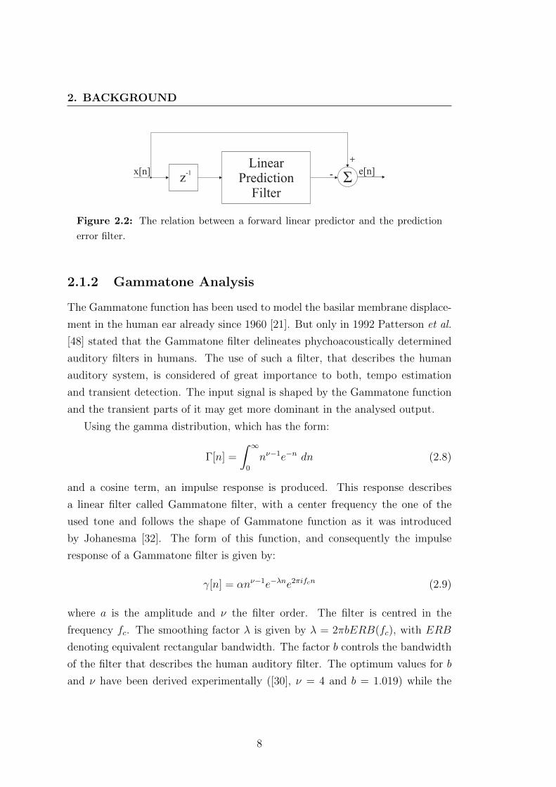
2.2 The relation between a forward linear predictor and the prediction

error filter. . . . . . . . . . . . . . . . . . . . . . . . . . . . . . . . 8

2.3 The impulse and frequency response of a Gammatone filter bank

with 16 channels. . . . . . . . . . . . . . . . . . . . . . . . . . . . 9

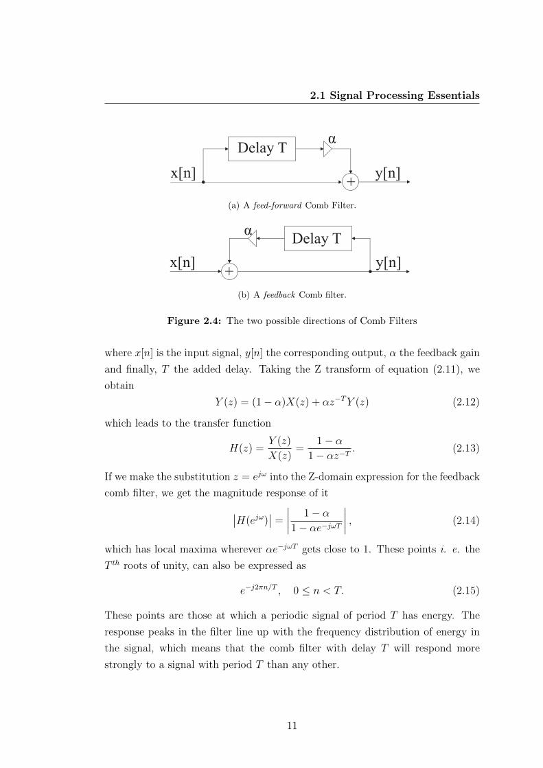
2.4 The two possible directions of Comb Filters . . . . . . . . . . . . 11

2.5 The relationships among beats in a 4/4 meter . . . . . . . . . . . 14

3.1 The general scheme of automatic Tempo Estimation . . . . . . . . 16

3.2 Attack, transient, decay and onset in the ideal case of a single note

[5] . . . . . . . . . . . . . . . . . . . . . . . . . . . . . . . . . . . 20

4.1 The block diagram of the proposed system. . . . . . . . . . . . . . 29

4.2 The general architecture of a filterbank that splits the input sig-

nal in M frequency bands and downsamples each band M times.

The processing is done separately in each frequency band before

upsampling and reconstructing the final output signal. . . . . . . 30

4.3 The block diagram of the feature list extraction method for a single

band of the input signal. . . . . . . . . . . . . . . . . . . . . . . . 31

4.4 The general architecture of a LMS adaptive filter . . . . . . . . . 33

4.5 The main parts of the peak-picking procedure . . . . . . . . . . . 37

4.6 The preprocessing of the DF before the peak-picking . . . . . . . 38

4.7 A bank of comb filters for frequency band k . . . . . . . . . . . . 39

xi

LIST OF FIGURES

4.8 The resonance model that was described in [45] to fit the distribu-

tions of responses to several pieces of music. . . . . . . . . . . . . 41

5.1 The Praat environment, used for the annotation of the sound test

files. . . . . . . . . . . . . . . . . . . . . . . . . . . . . . . . . . . 45

5.2 The predefined separation windows . . . . . . . . . . . . . . . . . 50

5.3 The average F-scores that the system achieved for the different test

cases. . . . . . . . . . . . . . . . . . . . . . . . . . . . . . . . . . . 52

5.4 The F-scores for the 6 test files for the optimum set of arguments. 53

5.5 Accuracy 1 on the Ballroom dataset. The literute algorithms men-

tioned are the following: Alonso [2], Dixon [17], Klapuri [35], Uhle

[57], and Scheirer [52]. . . . . . . . . . . . . . . . . . . . . . . . . 56

6.1 The block diagram of the proposed system. . . . . . . . . . . . . . 60

xii

List of Tables

5.1 The defined input arguments for the Transient Detection and Sep-

aration system. . . . . . . . . . . . . . . . . . . . . . . . . . . . . 48

5.2 The selected subset of arguments for which testing took place. . . 51

5.3 The results per file for the optimum set of arguments . . . . . . . 52

5.4 The Accuracy 1 of the algorithm for the estimation of the winning

tempi . . . . . . . . . . . . . . . . . . . . . . . . . . . . . . . . . . 54

5.5 Resulting percentages of the algorithm . . . . . . . . . . . . . . . 55

xiii

LIST OF TABLES

xiv

Chapter 1

Introduction

The last few years, users have a growing interest for new technologies that enable

them to enjoy music in a frequent basis. There are several reasons explaining this.

First of all, music is a universal form of art, that people can share and understand,

despite the barriers of national languages and cultural backgrounds. Moreover,

the advent of the technology in the field of music recording and reproduction

allows users to access music at a quality comparable to that of a live performance.

Music today is portable and accessible by a large group of the population that

seeks an auditory experience. The above reasons prove the importance of music,

in a cultural but also commercial context.

Music Information Retrieval(MIR) is an emerging research field, devoted to

fulfil the information needs that users of music have. MIR comprises a variety

of different applications, which aim at managing music, while making it more

accessible. A user study, that focuses upon real-time music information needs

[37], proves that users seek information to assist the building of music collections

and verify or identify musical excerpts, artists and lyrics. During these proce-

dures users value on-line music reviews, ratings and automatic recommendations.

MIR applications help music information seeking to become a public and shared

process, instead of being a private and isolated one.

There are several systems that access and retrieve music based on metadata,

i.e. textual descriptors. Such systems are mainly Digital Libraries, most of which

are devoted to Western music. Some popular examples are Cantate, Harmonica

and Musica. However, despite the emphasis on the retrieval part in the name

1

1. INTRODUCTION

of MIR, most of the research in this field and most of the systems this research

generated, are content-based. This means, that a music file is described by a set of

features that are directly computed by its content, with this term (i.e. content)

referring to the internal of an object, and being directly related to what this

object is. A basic assumption for content-based information retrieval approaches

is that metadata are for some reason unavailable. In audio standards (e.g. MP3),

metadata fields are usually not mandatory and even if these fields are present,

their quality and suitability relies on the creator of the file.

There is a strong motivation to design and develop systems that completely

rely on the content of the music files. These systems process directly the sound

signal to extract information that can be used by a great variety of applications.

Some examples of features that are used to obtain content-based representations

of music files, are audio onset and key detection, melody extraction, fundamental

frequency estimation, beat tracking and tempo estimation. MIR systems that

offer audio classification, query-by-humming, cover song identification and struc-

tural segmentation, are only a few of the systems that use the above features to

cover music information needs.

1.1 Scope of the Thesis

During the first half of the 19th century, the invention of the metronome, by

Johann Nepomuk Malzel, led to systematic mathematical markings for tempo

which, as time passed, became very popular. Beethoven was the first one to

use metronome markings for his symphonies, while others, like Bela Bartok and

John Cage, preferred to give the total time of a piece for a rough estimation of

the tempo. Today tempo is indicated in beats per minute (BPM) and with the

advent of modern electronics it became an extremely precise measure.

The process of automatically inferring the tempo of a musical piece plays an

important role among several applications in the field of MIR. Many of them, for

example beat tracking and music classification, need a preprocessing stage where

tempo estimation takes place. Beyond these, tempo induction is essential in mu-

sic similarity and recommendation, automatic transcription, even audio editing.

More complicated tasks such as meter extraction and rhythm description demand

2

1.1 Scope of the Thesis

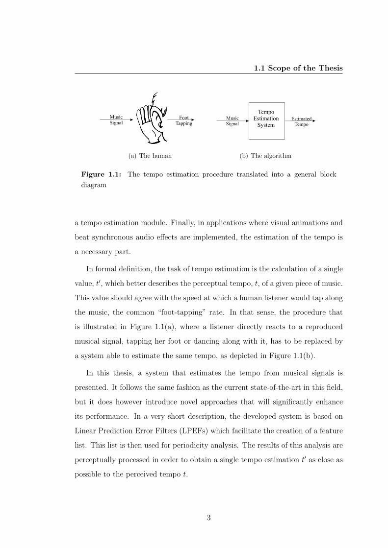
(a) The human (b) The algorithm

Figure 1.1: The tempo estimation procedure translated into a general block

diagram

a tempo estimation module. Finally, in applications where visual animations and

beat synchronous audio effects are implemented, the estimation of the tempo is

a necessary part.

In formal definition, the task of tempo estimation is the calculation of a single

value, t′, which better describes the perceptual tempo, t, of a given piece of music.

This value should agree with the speed at which a human listener would tap along

the music, the common “foot-tapping” rate. In that sense, the procedure that

is illustrated in Figure 1.1(a), where a listener directly reacts to a reproduced

musical signal, tapping her foot or dancing along with it, has to be replaced by

a system able to estimate the same tempo, as depicted in Figure 1.1(b).

In this thesis, a system that estimates the tempo from musical signals is

presented. It follows the same fashion as the current state-of-the-art in this field,

but it does however introduce novel approaches that will significantly enhance

its performance. In a very short description, the developed system is based on

Linear Prediction Error Filters (LPEFs) which facilitate the creation of a feature

list. This list is then used for periodicity analysis. The results of this analysis are

perceptually processed in order to obtain a single tempo estimation t′ as close as

possible to the perceived tempo t.

3

1. INTRODUCTION

1.2 Outline of the Thesis

The rest of the thesis is organised as follows. In Chapter 2 all the necessary ma-

terial for the understanding and justification of the implementation is described.

Working with music signals demands knowledge and processing tools inspired

from two main fields: Signal Processing and MIR. Therefore, this chapter focuses

on both of these domains. In Chapter 3 the existing literature on the field of

tempo estimation is presented. Existing algorithms are explained, discussed and

compared. During this review, important findings, that address problems in the

existing systems, are revealed and these are examined in the last part of the

chapter. The proposed method is thoroughly explained in Chapter 4. Each step

that is important for the whole architecture is presented, discussed and justified.

In Chapter 5 the developed system is evaluated. Apart from the results of the

evaluation that took place, the methods, data and metrics used for it are also

presented. Finally, this thesis concludes in Chapter 6 with the summary of the

work. The important bits and pieces of the whole thesis are gathered and rep-

resented in a reviewing chapter which also discusses possible extensions of this

work.

4

Chapter 2

Background

An MIR application uses knowledge from areas as diverse as signal processing,

machine learning, information and music theory. In this chapter, the theoretical

background, which provides necessary knowledge for understanding the content

of this thesis is presented. Firstly, certain Signal Processing tools used in various

parts of the implementation are introduced to the reader in Section 2.1. In the

second part of the chapter, Section 2.2, important aspects from Music Theory

and Music Signal Processing are described.

2.1 Signal Processing Essentials

2.1.1 Linear Prediction

A signal x[n] represents the realization of an autoregressive (AR) process of order

M, if it satisfies the difference equation

x[n] + a1x[n− 1] + ...+ aMx[n−M ] = v[n], (2.1)

where a1, a2, aM are constant values called AR parameters, x[n − k] is the kth

past value of the signal and v[n] white noise. An attempt to better understand

equation (2.1) may lead to rewriting it as

x[n] = −a1x[n− 1]− . . .− aMx[n−M ] + v[n]. (2.2)

5

2. BACKGROUND

� � �

�� ��

���

��

����

���

���

��� ��� � �� � � �� � � �� �� �

��� � �

� � � �� �

(a) A forward linear predictor.

� � �

�� ��

��

�� �

����

���

���

��� ��� � �� � � �� � � �� �� �

��� � �

� � � �� �

��

�

� � � � �

(b) A forward linear error predictor.

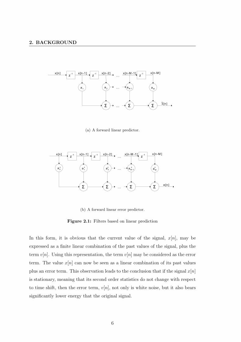
Figure 2.1: Filters based on linear prediction

In this form, it is obvious that the current value of the signal, x[n], may be

expressed as a finite linear combination of the past values of the signal, plus the

term v[n]. Using this representation, the term v[n] may be considered as the error

term. The value x[n] can now be seen as a linear combination of its past values

plus an error term. This observation leads to the conclusion that if the signal x[n]

is stationary, meaning that its second order statistics do not change with respect

to time shift, then the error term, v[n], not only is white noise, but it also bears

significantly lower energy that the original signal.

6

2.1 Signal Processing Essentials

Forward Linear Prediction Assuming that the current value of the signal

x[n] is unknown, and using the all-pole filter shown in Figure 2.1(a), we can

predict an approximation x[n] of x[n] where

x[n] =M∑k=1

akx[n− k]. (2.3)

In that case, the error between the actual value x[n] and the predicted value x[n]

is given by

e[n] = x[n]− x[n]. (2.4)

Forward Linear Prediction Error filter The forward linear predictor shown

in Figure 2.1(a), consists of M unit-delay elements and M tap weights, i.e AR

parameters, a1, a2, . . . aM that are fed with the respective samples x[n−1], x[n−2], . . . , x[n−M ] as inputs. The resulting output is the predicted value x[n], given

from the equation (2.3). Substituting this into equation (2.4), the prediction error

can be expressed as

e[n] = x[n]−M∑k=1

akx[n− k]. (2.5)

Denoting

a∗k =

{1 if k = 0

−ak if k = 1, 2, . . . ,M(2.6)

the equation (2.5) may be rewritten as follows

e[n] =M∑k=0

a∗kx[n− k]. (2.7)

From this form, it is obvious that, using the M + 1 tap weights a∗k and again M

unit-delay elements, we can create a filter which takes the signal x[n] as an input

and produces in the output the prediction error of the forward linear error filter.

Figure 2.1(b) shows the design of such a system, while Figure 2.2 illustrates the

relation between a forward linear prediction filter and a forward linear prediction

error filter.

7

2. BACKGROUND

LinearPrediction

Filter

-1z Σx[n] e[n]

+

-

Figure 2.2: The relation between a forward linear predictor and the prediction

error filter.

2.1.2 Gammatone Analysis

The Gammatone function has been used to model the basilar membrane displace-

ment in the human ear already since 1960 [21]. But only in 1992 Patterson et al.

[48] stated that the Gammatone filter delineates phychoacoustically determined

auditory filters in humans. The use of such a filter, that describes the human

auditory system, is considered of great importance to both, tempo estimation

and transient detection. The input signal is shaped by the Gammatone function

and the transient parts of it may get more dominant in the analysed output.

Using the gamma distribution, which has the form:

Γ[n] =

∫ ∞0

nν−1e−n dn (2.8)

and a cosine term, an impulse response is produced. This response describes

a linear filter called Gammatone filter, with a center frequency the one of the

used tone and follows the shape of Gammatone function as it was introduced

by Johanesma [32]. The form of this function, and consequently the impulse

response of a Gammatone filter is given by:

γ[n] = αnν−1e−λne2πifcn (2.9)

where a is the amplitude and ν the filter order. The filter is centred in the

frequency fc. The smoothing factor λ is given by λ = 2πbERB(fc), with ERB

denoting equivalent rectangular bandwidth. The factor b controls the bandwidth

of the filter that describes the human auditory filter. The optimum values for b

and ν have been derived experimentally ([30], ν = 4 and b = 1.019) while the

8

2.1 Signal Processing Essentials

101 102 103 104−50

−40

−30

−20

−10

0

10

20

Frequency (Hz)

Mag

nitu

de (d

B)

(a) The frequency response.

0 0.01 0.02 0.03 0.04 0.05 0.06 0.07 0.08 0.09

121

320

633

1124

1896

3108

5011

8000

Time (sec)

Cen

ter f

requ

ency

(Hz)

(b) The impulse response.

Figure 2.3: The impulse and frequency response of a Gammatone filter bank with

16 channels.

9

2. BACKGROUND

size of an ERB in the human auditory system has been estimated as ERB(fc) =

24.7 + 0.108fc [22] for median sound pressure levels. The impulse and frequency

responses of 16 filters that comprise a Gammatone filterbank are shown in Figure

2.3.

2.1.3 Comb Filters

A comb filter is a unit that adds a delayed version of a signal to itself. This

action results to interference, constructive or destructive, depending on the phase

difference upon addition. For example, if a wave A1 and its delayed version A′1

are in phase, then since they share the same frequency, their troughs and peaks

will line up and result to a wave with amplitude A = A1 + A′1 = 2A1. In

the opposite case, where the wave is not in phase with its delayed version, the

resultant amplitude is A = |A1 − A′1| = 0. In the more general case, where

the signal A1 is not a wave but an audio or music signal, the type of resulting

interference will not depend only on the relative delay, but also on the different

periodicities that appear locally on the input signal.

Mathematical Model The comb filters may be described in two different

ways, according to the direction in which signals are delayed before they are

added to the input. These two forms appear in Figure 2.4, and namely are feed-

forward and feedback.

Feed-forward The general structure of a feed-forward comb filter in shown

in Figure 2.4(a). It is described by the difference equation

y[n] = (1− α)x[n] + αx[n− T ], (2.10)

where x[n] is the input signal, y[n] the corresponding output, α the feed-forward

gain and finally, T the added delay.

Feedback The general structure of a feedback comb filter in shown in Figure

2.4(b). It is described by the difference equation

y[n] = (1− α)x[n] + αy[n− T ], (2.11)

10

2.1 Signal Processing Essentials

Delay T

x[n] y[n]

α

(a) A feed-forward Comb Filter.

x[n]

Delay T

y[n]

α

(b) A feedback Comb filter.

Figure 2.4: The two possible directions of Comb Filters

where x[n] is the input signal, y[n] the corresponding output, α the feedback gain

and finally, T the added delay. Taking the Z transform of equation (2.11), we

obtain

Y (z) = (1− α)X(z) + αz−TY (z) (2.12)

which leads to the transfer function

H(z) =Y (z)

X(z)=

1− α1− αz−T

. (2.13)

If we make the substitution z = ejω into the Z-domain expression for the feedback

comb filter, we get the magnitude response of it∣∣H(ejω)∣∣ =

∣∣∣∣ 1− α1− αe−jωT

∣∣∣∣ , (2.14)

which has local maxima wherever αe−jωT gets close to 1. These points i. e. the

T th roots of unity, can also be expressed as

e−j2πn/T , 0 ≤ n < T. (2.15)

These points are those at which a periodic signal of period T has energy. The

response peaks in the filter line up with the frequency distribution of energy in

the signal, which means that the comb filter with delay T will respond more

strongly to a signal with period T than any other.

11

2. BACKGROUND

2.2 Music Structure, Hierarchy and Perception

Most of the approaches and techniques used for MIR applications are based on

a number of music concepts that may not be familiar to readers without musical

training. This section will present a short introduction to such concepts and

terms.

2.2.1 Basic Music Elements

The musical instruments produce almost periodic vibrations, with percussive in-

struments being the only exception to that. A sound produced by a musical

instrument is a combination of various frequencies, all of which are integer mul-

tiples of a fundamental frequency.

A basic feature, which is directly related to the perception of the fundamental

frequency, is the pitch. Although pitch is closely related to frequency, the two are

not equivalent [35]. Frequency is an objective, scientifically measurable concept,

whereas pitch is subjective. Sound waves themselves do not have pitch, and their

oscillations can be measured to obtain a frequency. It takes a human brain to

map the internal quality of pitch and range a musical piece from low or deep to

high or acute sounds.

Another basic music element is the intensity. Intensity is related to the

amplitude, and thus to the energy of the vibration and may also be defined as

the loudness. Therefore intensity may range from soft to loud.

When two sounds are of the same pitch and intensity listeners are still able to

perceive them as different when these two sounds have a different timbre. Tim-

bre, also called tone quality or tone colour, mediates from physical characteristics

of sound such as its spectrum and envelope.

Regarding the perception of the above elements, pitch and intensity are not

perceived in as a straightforward way as the above definitions may imply. The

behaviour of the human ear is not linear. However, it is possible to approximate

the perceptually relevant qualities of them, taking into consideration the funda-

mental frequency and the energy of the sound. On the other hand, timbre is a

multidimensional sound quality that is related to the recognition of the sound

source, but cannot be described with simple features.

12

2.2 Music Structure, Hierarchy and Perception

In the case of percussive instruments, as mentioned above there is no fun-

damental frequency, and the sound is usually called noise. The noisy parts are

still perceived as low, medium or high, so intensity and timbre are still relevant

descriptors.

2.2.2 The Metrical Structure of Music

When listening to a piece of music, humans instinctively infer regular patterns of

strong and weak beats. The actual musical content relates to these patterns and

listeners tap their feet along to the music. The term used for these patterns of

beats is meter. Generalizing, the regular hierarchical pattern of beats to which

the listener relates musical events to, is called metrical structure.

Following the terminology used in [38], a first term associated to the metrical

structure of music is the accent. It is often used in connection with meter and it

has gained a lot of attention in the field of automatically description of it. Three

kinds of accent are distinguished:

1. Phenomenal Accent is any event at the musical surface (i.e. attacks or

sudden changes) that emphasizes moments in the musical flow.

2. Structural Accent is caused by melodic or harmonic, sudden events.

3. Metrical Accent is any beat, relatively strong in its metrical level.

An important relation between the above kinds of accent is that phenomenal

accent functions as a perceptual input to metrical accent. In other words, the

moments of musical stress in a music signal, are used by a human listener to

extract a regular pattern of metrical accents. If phenomenal accent is not regular,

the perception of metrical structure becomes ambiguous.

Metrical patterns consist of elements called beats. Beats do not have dura-

tion, they are temporal points that performers utilize and listeners infer. A fun-

damental concept of musical meter is the periodic alternation between “strong”

and “weak” beats. To achieve so, a metrical hierarchy, consisting of two or more

beat levels, exists in every musical sound. When a beat is felt to be stronger than

other beats (of the same metrical level) then it is also a beat at the higher level.

13

2. BACKGROUND

Beats 1 2 3 4 1 2 3 4 1

tatumtactusmeasure

Figure 2.5: The relationships among beats in a 4/4 meter

In Figure 2.5 such an example is presented. In this Figure, a 4/4 meter is de-

picted, where the first and third beats are felt to be stronger than the second and

fourth. It is important to note that the beats in Figure 2.5 are equally spaced,

not only at the first level, but also at the higher ones. The term meter implies

measuring of fixed intervals and distances.

In the above description of the hierarchical structure of musical meter, the

most prominent level, the one at which the conductor waves his baton and the

listeners taps his foot is the tactus. This is illustrated as the second level in Figure

2.5. One level below, is the tatum level, a name stemming from “temporal atom”

as the period of the beats in this level is the shortest that is encountered. The

remaining higher level is often called measure, related to the length of a rhythmic

pattern. “Well-formedness” rules for music demand that every metrical level,

strong beats are spaced either two or three beat apart, while beats at the tactus

level, or above, should be equally spaced throughout the piece. The tempo of a

piece is defined as the rate of the tactus beats.

14

Chapter 3

Literature Review

In this chapter the most important findings in the field of tempo estimation

are presented. An extended literature review revealed a general scheme that is

followed by most tempo induction algorithms. In Section 3.1 this general archi-

tecture is presented with references to popular algorithms that either established

or proved the importance of using certain tools. As described there, the first

step of this architecture often relies on the detection of musical events. The term

musical events is used to describe onsets, transients and attacks that take place

in the temporal evolution of the signal. Literature that concerns the detection

of such events is presented in Section 3.2. Finally, Section 3.3 discusses issues

that have been revealed during the review of existing methods. These issues are

important for an attempt to resolve the problems that these methods have and

to develop an accurate tempo estimation method.

3.1 Tempo Estimation

The tempo is a dominant element connected to the hierarchical structure of a

music signal that can define various aspects of it. Moreover, it is an intuitive

music property that human listeners, even without any musical education are

able to perceive and understand only by listening to the first few seconds of an

excerpt. The tempo is defined as the rate of the tactus pulse, a prominent level

in the hierarchical structure of music, which is also referred to as the foot-tapping

rate.

15

3. LITERATURE REVIEW

Feature List Extraction

TempoInductioninput

signalfeature

listestimated

tempo

Figure 3.1: The general scheme of automatic Tempo Estimation

In the literature, systems that conduct tempo estimation present a variation

on the type of input signals they use. Older systems [10, 42] deal with symbolic

data (Musical Instrument Digital Interface - MIDI) or manually parsed scores

that contain only onset times and durations. More recent systems on the other

hand, tend to use directly the audio, or even the compressed, signal [60]. There

are some cases though that newer systems use a MIDI input [16, 49] and older

ones use audio input [11, 53]

Regardless the type of the input data they use, tempo induction algorithms

usually follow a general scheme [25, 26], that consists of two main stages and is

depicted in Figure 3.1. In the first stage, the audio signal is parsed, or filtered, into

a sequence of features. During the second stage of the tempo induction scheme,

fundamental periodicities of the feature lists are highlighted and the tempo is

inducted.

3.1.1 Feature List Creation

Several methods have been proposed in the literature for the task of extracting

feature lists, adequate for tempo estimation systems. A short description of

the most important and widely used among these methods is given in the next

paragraphs.

Onset Times & Inter-Onset Intervals (IOIs) The use of onset times for

tasks related to rhythmic analysis is very common in the literature. There has

been extended research in the task of onset detection, that is reviewed in Section

3.2. In addition to the exact times at which onset events take place, several

systems make use of the IOIs. Some representative algorithms of this category,

that make use of onsets and IOIs for the extraction of a feature list may be found

16

3.1 Tempo Estimation

in [10, 42, 47]. Some more recent and quite accurate algorithms of this category

are [2, 14].

Relative Amplitude The relative amplitude is easily estimated from the audio

signal (of MIDI data if these are used). Although it is a factor that contributes

to the perceptual accentuation, score notation is largely absent from it. However,

relative amplitude is used by various systems for weighting reasons [15, 17].

Pitch Pitch is another feature easily extracted from MIDI data or even scores.

However, it gets difficult to obtain it from polyphonic signals. It has not been

regularly used, with an exception in [16], where pitch is extracted along with

duration and amplitude from MIDI data. The above are used for the calculation

of the “salience” of musical events.

Percussive Events Drum sounds are considered by several authors as cues

that indicate the hierarchical structure of music [23, 27]. It is rather easy to

extract this information from MIDI data or monophonic music signals (isolated

percussions) but their recognition is still under research in the polyphonic music.

The detection of transient events, which are the source of percussions, is described

in Section 3.2.

Frame Features In this category the algorithms use features that are extracted

directly from the audio signal. These features may emphasize onset locations but

they do not result from onset lists. In [52] an amplitude envelope of the signal

in six octave-spaced subbands is created at the first stage of the system. This

approach is expanded in [35], where a more generic and therefore robust accent

signal is created across four subbands.

3.1.2 Pulse Induction

During the second stage of the tempo induction scheme is when pulse induction

takes place. A pulse, or metrical level, is defined here as a periodic recurrence of a

certain feature in time. This stage aims in emphasizing the periodic behaviours of

the features lists so that pulse periods are estimated. An important assumption

17

3. LITERATURE REVIEW

is made at this stage: the pulse period should be constant over the data used for

its computation.

Two main procedures can be found in the literature for pulse induction,

namely pulse selection and periodicity function computation.

Pulse Selection The first approach to pulse induction assumes that each found

IOI defines a possible pulse period and the corresponding events define the phase.

In [42] the two first events in an onset list are considered to be the two first pulses

while in [12] the first two agreeing IOIs define the pulse. It is also possible to

seek periodic behaviours in the feature list by computing a similarity measure

between the list and several pulse track. Although several authors have followed

this approach for pulse induction, current state-of-the-art systems generally follow

the approach described next.

Periodicity Function Computation The second approach to pulse induction

is the computation of a periodicity function which assigns a specific salience in

each frequency that appears. These functions are often calculated with standard

signal processing algorithms, such as Fourier transform applied on onset lists [8].

In [54] wavelets are used to capture temporal organizations at different hierar-

chical levels. Nevertheless, the most common signal processing tool used for the

computation of the periodicity function is the autocorrelation function (ACF)

[17, 23, 27, 56, 57]. This may be computed from a wide range of different input

data, for example sequences of (weighted or not) onsets [10, 51]. An alternative

approach to ACFs uses a bank of resonators, each tuned to a different possible

periodicity. The output of each resonator indicates the strength of the input in

the corresponding period. In [52] comb filter resonators are used separately in 6

frequency sub bands of the input signal. In [35] comb filter resonators are also

used while in [36] phase-locking resonators are proposed.

3.2 Event Detection in Music Signals

The detection, modelling and separation of certain events that appear in music

signals are of great importance to a wide range of audio signal processing algo-

18

3.2 Event Detection in Music Signals

rithms. The term event, is used here to describe onsets, transients and attacks.

The detection of these attempts to locate the onsets of any percussive instru-

ments and it can be used in tasks such as tempo estimation, beat tracking and

automatic transcription. Algorithms for audio editing, content delivery and in-

dexing also need a transient detector. Moreover, as a subset of the automatic

event detection algorithms, transient detection techniques give new possibilities

to a wide range of music applications, including content delivery, compression,

indexing and retrieval [5].

Correctly detecting and identifying musical events is of critical importance for

accurate music information retrieval algorithms. The available literature on the

topic includes many different approaches for detecting onset, transient and attack

parts in a music signal. An attempt to implement a system able to fully detect

drum parts in an audio recording should be approached as any other system of

musical events detection. As drums may be considered as a subset of the transient

events of an audio recording it is important to study the available literature in

topics such as detection of onsets, transients and attacks.

3.2.1 Definitions: Transients, Attacks and Onsets

The similarities between terms transients, onset and attack are many and the

differences rather vague. Due to the difficulty to precisely define what a transient

is, only an informal description of transients can be given. In general, transients

are short intervals during which the signal evolves quickly in some non-trivial or

relatively unpredictable way. Even if the start time of a transient can easily be

found with the time representation of a signal, it is still quite difficult to localize

its end. Usually the duration of the transient is considered to be the duration

during which new frequencies exist in the spectrum of the signal.

Quite similar to the term transient, are the terms onset and attack. A lot of

algorithms developed for the detection of transient parts within a music signal

give quite satisfactory results for the detection of onsets and attacks, and vice

versa. However, it is necessary to distinguish these three concepts. Onset of a

note is called the exact time that this note begins, but this time is not always the

starting point of a transient. Once a new note has been introduced in a music

19

3. LITERATURE REVIEW

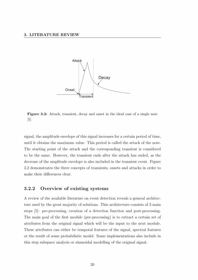
Figure 3.2: Attack, transient, decay and onset in the ideal case of a single note

[5]

signal, the amplitude envelope of this signal increases for a certain period of time,

until it obtains the maximum value. This period is called the attack of the note.

The starting point of the attack and the corresponding transient is considered

to be the same. However, the transient ends after the attack has ended, as the

decrease of the amplitude envelope is also included in the transient event. Figure

3.2 demonstrates the three concepts of transients, onsets and attacks in order to

make their differences clear.

3.2.2 Overview of existing systems

A review of the available literature on event detection reveals a general architec-

ture used by the great majority of solutions. This architecture consists of 3 main

steps [5]: pre-processing, creation of a detection function and post-processing.

The main goal of the first module (pre-processing) is to extract a certain set of

attributes from the original signal which will be the input to the next module.

These attributes can either be temporal features of the signal, spectral features

or the result of some probabilistic model. Some implementations also include in

this step subspace analysis or sinusoidal modelling of the original signal.

20

3.2 Event Detection in Music Signals

Having obtained a set of features that can be used for transient detection,

the next step is to create an appropriate detection function. In most of the cases

this function is a highly subsampled function that follows the spectral or time

envelope of the original signal, having local maxima (peaks) around the region of

the appearance of a transient. These peaks are often masked by noise, making

it rather difficult for any peak-picking algorithm to locate them in the detection

function. The selected peak-picking algorithm must be as robust as possible.

Once the peaks have been extracted from the detection function, the locations

of the appearance of transient events in the signal are known. During the post

processing each application handles these detected transients according its needs.

Since this step of post processing is quite application-oriented any generalization

of it would be beyond the need of the current description.

3.2.2.1 Preprocessing

An optional step which consistently appears in the literature is the preprocessing

step, which aims in accentuating or attenuating aspects of the signal so that

the task in hand is simplified. There is a wide range of preprocessing modules,

however there are two methods that appear to be more popular than the rest of

them: subspace analysis and transient/steady-state separation.

Subspace Analysis The analysis in several frequency bands has been found to

be useful in a wide range of algorithms. Among these algorithms, we can discern

two main categories: one that consists of the system that need the subspace

analysis in order to produce global estimates on the transients and one that

consists of systems that aim in improving the robustness of the system by breaking

down the analysis into several bands. As an example of the systems falling into

the first category, in [24] a multiple-agent architecture is used. This architecture

detects rhythmic structure in music, and the analysis into several frequency strips

is of great importance to recognize sudden changes in energy. Moreover, in [52] a

sixth-order elliptic filter is used for the implementation of a six-band filter bank.

Onset trains are then created, via a psychoacoustically inspired processing, which

are fed into comb-filter resonators estimating that way the tempo of a signal.

21

3. LITERATURE REVIEW

In the second category, belong systems as the one presented in [34] where a

filter bank divides the spectrum into 8 non-overlapping bands. In each band,

onset times and intensities are calculated and then combined so that the human

auditory cochlea is approximated. Another system of this category is described

in [3], where a short time Fourier Transform is used in order to separate the signal

in different frequencies and then assign a percussivity measure to short frames of

every frequency bins.

Transient/steady-state separation The processes using transient/steady-

state separation produce modified signals, such as residuals and/or transient

signals for the purpose of onset detection. One group of approaches that fall

into this category make use of sinusoidal models, such as in [44]. The audio

signal is represented as a sum of sinusoids and noise. Levine in [40] calculates

the residual between the original signal and a spectral modelling synthesis model.

Following this approach, any significant increases in the energy of the residual

imply a mismatch between the model and the signal, a fact that successfully high-

lights existing onsets. An extension of spectral modelling synthesis, the transient

modelling synthesis, is presented in [59]. Transient signals are analysed there by

a sinusoidal analysis/synthesis scheme, on the discrete cosine transform of the

residual.

3.2.2.2 Detection Function Creation

The process of transforming the audio signal to a highly subsampled detection

function is possibly the core of the transient/onset detection algorithms. The de-

tection function may be created with algorithms inspired by two different general

approaches: use of predefined signal features or probabilistic signal models. In

any case the resulting detection function will manifest the occurrence of transients

in the input signal.

Predefined signal features In the time domain, when observing the evolution

of simple musical signals, it is noticeable that the occurrence of an onset is usually

accompanied by an increase of the signal’s amplitude.The technique of following

the amplitude envelope of the signal dominated in the early methods of onset

22

3.2 Event Detection in Music Signals

detection. This operation could be easily done by rectifying and smoothing the

signal in time domain representation. A variation on this is following the local

energy, instead of the amplitude, by squaring the signal during the calculation.

Even after the smoothing, though, these signals (amplitude or energy enve-

lope) cannot provide a stable onset detection function. For that reason, a great

number of onset detection studies used the derivative of the energy. In that way,

any sudden changes in the energy are translated into narrow peaks in the deriva-

tive function. This method in combination with filter-bank analysis is employed

in [24] while in [40] and [20] is used with transient/steady-state separation.

Finally, psychoacoustics may be used for further improvement on the detec-

tion functions. Empirical evidence, as described in [46] proves that loudness is

perceived logarithmically. This means that the calculation of the logarithm of

the signal’s energy will simulate the ear’s perception of loudness. Such an imple-

mentation in multiple bands is described in [34].

Moving now to the frequency representation of the signal, a lot of applications

have been designed that use spectral features for onset/transient detection. This

reduces the need for pre-processing while is quite useful when it comes to poly-

phonic music and instruments discrimination. In the spectral domain, energy

increases linked to transients tend to appear as a broadband event. However,

since the energy of the signal is usually concentrated at low frequencies, changes

due to transients are more noticeable at high frequencies. Using this knowledge

the spectrum of the signal (obtained via a short time Fourier transform) may be

weighted toward the high frequencies [50]. In that way a detection function that

also exhibits peaks where transient information is located, is obtained.

Also in the frequency domain, [43] uses the L1-norm of the difference between

magnitude spectra, while [20] uses the L2-norm on the rectified difference. Finally,

certain approaches [6, 7, 19] make use of the phase spectra of the signal to obtain

extended information on the behaviour of onsets. This can be justified taking

into consideration that much of the temporal structure of a signal is encoded in

the phase spectrum.

Another approach [29], introduces onset detection based on the phase spec-

trum and specifically using the average of the group delay function. A frame

based analysis of a music signal provides the evolution of group delay over time,

23

3. LITERATURE REVIEW

creating a phase slope function. Onsets are may be detected simply by locating

the positive zero-crossings of the phase slope function.

Probabilistic Models Assuming that the signal may be described by some

probability model, statistical methods for onset/transient detection have been

developed. The success of such models depend in a high level on the ability

of the model to fit to the real distribution of the signal. Likelihood measures

or Bayesian selection criteria may be used for the quantification of the system’s

success.

A quite robust and well known probabilistic approach is based on the sequen-

tial probability ratio test [4]. Assuming that the signal samples are generated

from one of two statistical models and defining the log-likelihood ratio, the ex-

pectation of the observed log-likelihood ratio depends on which model the signal

is actually following. In this context, the log-likelihood ratio can be considered

as a detection function that will present changes in polarity, as its detectable fea-

ture. Algorithms presented in [31, 55], apply variation of the above method, using

parametric Gaussian autoregressive models for the estimation of the statistical

models.

3.2.2.3 Post-processing

If the above described parts of a transient (or onset) detection system are properly

designed and implemented, the produced detection function will exhibit certain

attributes indicating the appearance of the events to be detected. These features

are local maxima in the most common case. Their shape and size is of course

variable and they are normally masked by noise. Therefore a robust peak-picking

algorithm is needed for estimating the actual times of events.

The peak-picking in the detection function may be further divided in three

steps: post-processing, thresholding and the decision making process. Based on

the exact method used to produce the detection function, the post-processing

step is necessary for improving the efficiency of the peak-picking procedure. The

noise may be reduced here via a smoothing actions while normalization may help

the selection of the thresholding arguments.

24

3.3 Conclusions

Even after post-processing, there will be a number of peaks in the detection

function which are not related to the events to be detected. Hence, it is nec-

essary to define a threshold which effectively separates event-related and non

event-related peaks. This threshold may be implemented using either fixed or

adaptive thresholding. In fixed thresholding only peaks that exceed the prede-

fined threshold may be considered as onsets. Although this approach performs

well when the music does not exhibit significant loudness changes, this is not the

usual case and therefore it tends to miss onsets in the most quiet parts. Using

adaptive thresholding [20, 46] on the other hand overcomes this problem, but

tends to mask any silent onsets that appear near a louder one.

After post-processing and thresholding the detection function, the task of

peak-picking is reduced in identifying local maxima above the defined, static or

adaptive threshold. In [33] an extended review on peak-picking algorithms for

audio signals is available.

3.3 Conclusions

While studying the available literature in the topic of tempo estimation for poly-

phonic music signals, several issues are revealed. It is important to underline

these issues, as their examination and correct approach will lead to an efficient

method, able to accurately induct the perceived tempo.

Selection of feature list extraction method Although algorithms that se-

lect low-level frame features for the computation of the feature list have been

found more noise-robust and in cases more accurate, it is still under discussion

whether this is perceptually more valid. The perception of tempo is considered

to be a redundant procedure that expands in many different levels. An ideal

system should take into consideration as many of these levels as possible during

the selection of the method for extracting the feature list. This however would

significantly raise the computational complexity of the whole system. Is this a

trade-off we have to accept or is there a way to gain information for more than

one levels, while keeping the algorithm simple?

25

3. LITERATURE REVIEW

Improving the existing algorithms Different systems seem to work well in

different data sets. This poses the question whether we should try and built

even more complex systems or it is enough to merge the existing ones, somehow

combining their output. The answer seems to be that a “smart” combination

will improve the global tempo estimation. This would also mean that an extra

processing step in the general tempo estimation architecture, could be useful for

a variety of systems.

Tolerance Window A tolerance window is systematically used in the literature

when it comes to the evaluation of tempo induction and event detection systems.

This is motivated by the fact that the evaluation of these algorithms highly

depends on ground truth data, which is obtained using hand labelling techniques.

Such techniques are ambiguous. In systems that detect musical events, 50ms is

a widely accepted tolerance window as it coincides with the just noticeable inter-

onset interval. Since beat pulses appear on onset times, this interval of 50ms

corresponds to a percentage range 3.3% - 20% (for periods range 40 to 240 BPM).

The choice of 4% tolerance window seems to be widely accepted in the literature.

Frequency Decomposition It is depicted in the literature that it is rather

important to apply frequency decomposition in the input signal. It is not yet

clear how (and whether) the exact choice of decomposition affects the results.

There are a few different approaches to this topic: the subspace analysis may

happen before or after the feature list extraction, in a few or more frequency

bands and with a wide range of different filterbanks.

Concluding this literature review in the topic of machine emulation of human

tempo induction, it becomes clear that it is still an open issue. Although there

are algorithms performing very well in some subsets of huge datasets, they fail to

do so globally, for any musical genre.

Moreover, existing systems need a long musical excerpt in order to give a

reliable tempo estimation. Many applications, though, demand instant estima-

tion available at the about the same time as a human listener would detected.

An algorithm able to induct perceived tempo, accurately, globally, using only a

26

3.3 Conclusions

short part of the input signal, is still missing from the literature. These are the

attributes that the proposed algorithm tries to achieve.

27

3. LITERATURE REVIEW

28

Chapter 4

Proposed Method

Human perception of tempo is considered to be redundant, expanding at many

levels [9]. The recognition and processing of points where abrupt changes take

place at the temporal evolution of a signal i.e. transient events, has been ex-

tensively discussed to be one of these levels. We propose the use of an adaptive

LPEF that enables the accentuation of such points. Prior to that, the use of a

Gammatone filterbank will model the input signal using a frequency resolution

that is similar to that of the human auditory system, enhancing that way the

estimation of the perceptual tempo.

A block diagram of the proposed system is shown in Figure 4.1. As depicted

there, three major units comprise the final architecture each of which is described

in details in the following sections of this chapter. The developed system follows

the general scheme of tempo estimation algorithms as this was presented in Sec-

tion 3.1. Subspace analysis, the first step of many tempo induction techniques

(including the proposed one), is omitted in this general scheme but it is explained

in the detailed description of the proposed method, in Section 4.1. After that,

in Section 4.2 the processing that takes place for the extraction of the feature

Feature List Extraction

Tempo Induction

PerceptualModelling

feature

list

winning

tempiestimated

tempoinputsignal

Figure 4.1: The block diagram of the proposed system.

29

4. PROPOSED METHOD

h [n]0

h [n]1

h [n]M-1

SUBBAND

PROSECCING

g [n]0

g [n]1

g [n]M-1

Μ

Μ

Μ

Μ

Μ

Μ

...... ... ...

Σx[n] y[n]

Figure 4.2: The general architecture of a filterbank that splits the input signal in

M frequency bands and downsamples each band M times. The processing is done

separately in each frequency band before upsampling and reconstructing the final

output signal.

list is presented. Pulse induction, the next step on the general architecture of

tempo estimation systems, is discussed in Section 4.3. In addition to these, a

last step where perceptual processing of the results takes place is integrated in

the proposed algorithm. This step is not a part of the general tempo estimation

scheme, but gives promising results. It is presented in Section 4.4 and it is based

on a resonance model that has been found to follow the perceptual responses to

a variety of musical excerpts [45].

4.1 Subspace Analysis

To analyse an audio signal using Gammatone signal models, a corresponding

signal processing unit has to be defined. This unit follows the general architecture

of a filterbank shown in Figure 4.2 and consists of K Gammatone filters of impulse

responses hk[n], k ∈ [0, K − 1].

The bandpass analysis output signals,

sk[n] = hk[n] ? x[n] =L−1∑m=0

x[n−m]hk[m], k = 0, 1, . . . K − 1, (4.1)

30

4.2 Feature List Extraction

Feature List Extraction

Linear Prediction Error Filters

Peak Picking Window Application

x [n]k m [n]kdf [n]kts [n]k

Figure 4.3: The block diagram of the feature list extraction method for a single

band of the input signal.

where L the order or the filter, are decimated by a factor of K, resulting to the

subband sequences

xk[n] = sk[Kn] =L−1∑m=0

x[Kn−m]hk[m], k = 0, 1, . . . K − 1, (4.2)

which comprise a critically sampled signal representation.

The used bank of filters splits the full band signal x[n] into K frequency bands.

In our implementation K was selected to be 16, a number of bands large enough

to have a good frequency resolution maintaining comparably low computational

complexity. In the same fashion and in order to reduce the computation com-

plexity, the equation (4.1) may also be implemented in the frequency domain,

using Fourier Transform

Sk(ejω)

= X(ejω)Hk

(ejω). (4.3)

where Sk (ejω), X (ejω), Hk (ejω) the Fourier representations of the corresponding

time signals, sk[n], x[n], hk[n].

4.2 Feature List Extraction

The process of feature list extraction, follows the architecture shown in Figure

4.3. As illustrated in this figure, there are three main modules that lead to the

creation of a set of signals, that are called mask functions and represent the

feature list for different critically sampled sub bands of the input signal.

31

4. PROPOSED METHOD

4.2.1 Detection Function Determination using Linear Pre-

diction

This module is the key process for transient detection. The goal is to obtain

a highly subsampled intermediate signal called detection function, DF, which

reveals the occurrences of transients in the original signal. The implementation

of this part is based on linear prediction (LP).

The application of LP assumes the signal to be stationary. This does not hold

when audio signals are used. In order to solve this problem it is necessary to

assume local stationarity over the signal. Every shorter part, even the transient

parts of the signal are considered as locally stationary parts. During the analy-

sis the application of a short window ensures that the currently processed part

(frame) is stationary. However, if the frame length of the analysis is a predeter-

mined constant number it is most probable that some frames will contain more

than one locally stationary segments of the signal, leading to a poor modelling

of these parts. Based on this idea, an LP based algorithm has been implemented

for the detection of transient parts within an audio signal.

The design of an adaptive LPEF for the detection of transient events

Using the linear prediction error filter (Figure 2.1(b)) the output error signal is

white noise of low energy if the input signal is stationary. If the window size

(which is used when obtaining a short frame of the input), is of a predefined

fixed length, then there will be some frames where the short frame will not be

stationary (due to poor modelling) and the linear prediction will fail to give good

results. During transient parts, where sudden changes happen to the input signal,

the prediction has poor results so this non stationarity is apparent in the residual

signal.

There are several ways to compute the linear prediction coefficients. In this

case, a long frame in time is analysed with the LP approach and for that reason an

adaptive algorithm based in Least-Mean-Squares (LMS) has been developed. This

algorithm updates the tap weights (a∗k) with time after their initial calculation,

which is done with the use of Levinson-Durbin algorithm.

32

4.2 Feature List Extraction

LMSAlgorithm

TraversalFilter

LMS

x[n] x[n]~

-

d[n]

+

Σ

Figure 4.4: The general architecture of a LMS adaptive filter

The Levinson-Durbin Algorithm One of the most efficient methods for com-

puting the linear prediction error filter coefficients is the Levinson-Durbin algo-

rithm. In order to give the optimum values for the tap weights of the filter, the

Levinson-Durbin algorithm solves the augmented Wiener-Hopf equations. The

algorithm was described firstly by Levinson [41] in 1947 and then independently

by Durbin [18] in 1960.

The adaptive LMS algorithm The least-mean-squares (LMS) algorithm is

a very simple linear adaptive filtering algorithm, a standard and widely used

method in the field of adaptive filtering [28]. The LMS algorithm consists of two

basic processes: a filtering process and an adaptive process. The filtering process

is the one that computes the output of a traversal filter produced by a set of tap

weights and generates the estimation error by comparing this output to a desired

response. The adaptive process on the other hand, takes the responsibility to

automatically adjust the tap-weights according to the computed estimation error,

minimizing the mean square value of it.

Figure 4.4 illustrates these parts of the LMS mechanism. The signal x[n] is

used as an input to the traversal filter, and an estimation of the desired response,

d[n] is produced, denoted as d[n]. According to the estimation error, e[n] the LMS

33

4. PROPOSED METHOD

algorithms undertakes the update of the tap weights of the filter. The adaptive

iteration that is used to achieve this is written as

• Filter output

d[n] = wT [n]x[n] (4.4)

• Estimation error

e[n] = d[n]− d[n] (4.5)

• Tap-weight adaptation

wT [n+ 1] = wT [n] + µe[n]x[n], (4.6)

where wT [n] = (a1, a2, ...aM) are the coefficients of the filter and x[n] = (x[n −1], x[n − 2], ..., x[n −M ])T are M values of the input signal. According to nor-

malized LMS the step size µ is chosen to be

µ = min

(a,

1

xT [n]x[n]

), (4.7)

where a is a small value preventing the step size to become too big when the

value xT [n]x[n] approaches zero.

In our approach, the traversal filter used is a linear prediction filter. The

desired response that is needed is set to be the current value of the input signal

(that means that the estimation error e[n] is the output of a linear prediction

error filter). The input vector to the system, x[n], consists of the M past values

of the input signal, x[n] = (x[n− 1], x[n− 2], . . . , x[n−M ])T

Summary of the adaptive LPEF Until now, the signal has been analysed

into several subbands, preprocessed and separated into short frames. Each frame

is then processed with an adaptive LPEF, that uses the Algorithm 1. In this

notation, x[n] is a vector of M values of the processed frame (which length is N),

while w[n] is a vector with the current tap-weights of the LPEF. The call of the

function LPC illustrates the initialization of the vector using the Levinson-Durbin

algorithm.

After running this routine for each frame of each band of the input signal, we

obtain a set of signals, ek[n], where k = 1, . . . , K − 1 corresponds to a certain

34

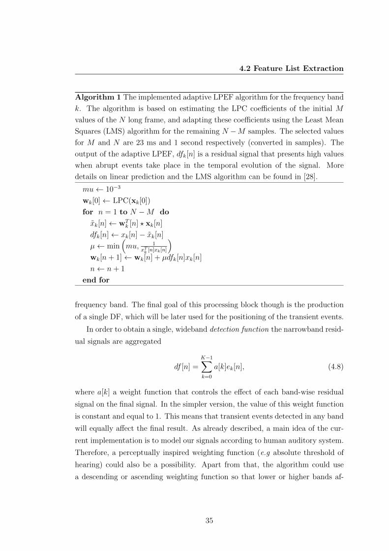
4.2 Feature List Extraction

Algorithm 1 The implemented adaptive LPEF algorithm for the frequency band

k. The algorithm is based on estimating the LPC coefficients of the initial M

values of the N long frame, and adapting these coefficients using the Least Mean

Squares (LMS) algorithm for the remaining N −M samples. The selected values

for M and N are 23 ms and 1 second respectively (converted in samples). The

output of the adaptive LPEF, dfk[n] is a residual signal that presents high values

when abrupt events take place in the temporal evolution of the signal. More

details on linear prediction and the LMS algorithm can be found in [28].

mu← 10−3

wk[0]← LPC(xk[0])

for n = 1 to N −M do

xk[n]← wTk [n] ? xk[n]

dfk[n]← xk[n]− xk[n]

µ← min(mu, 1

xTk [n]xk[n]

)wk[n+ 1]← wk[n] + µdfk[n]xk[n]

n← n+ 1

end for

frequency band. The final goal of this processing block though is the production

of a single DF, which will be later used for the positioning of the transient events.

In order to obtain a single, wideband detection function the narrowband resid-

ual signals are aggregated

df [n] =K−1∑k=0

a[k]ek[n], (4.8)

where a[k] a weight function that controls the effect of each band-wise residual

signal on the final signal. In the simpler version, the value of this weight function

is constant and equal to 1. This means that transient events detected in any band

will equally affect the final result. As already described, a main idea of the cur-

rent implementation is to model our signals according to human auditory system.

Therefore, a perceptually inspired weighting function (e.g absolute threshold of

hearing) could also be a possibility. Apart from that, the algorithm could use

a descending or ascending weighting function so that lower or higher bands af-

35

4. PROPOSED METHOD

fect strongly the output. The latter would be useful for detection of bandwise

transient events (or transcription of different percussive sounds, as snare drums).

4.2.2 Peak-picking

The output of the adaptive linear prediction filter, described in Section 4.2.1, is a

function that presents local maxima when abrupt events take place in the input

signal. These peaks are subject to some level of variability in shape and size due

to noise or other aspects in the initial signal. In order to determine which of

these peaks are related to transient events, a robust peak-picking algorithm is

needed. This module will take as an input the DF produced from the LPEF filter

and will produce a time series that localize the transients onsets into the initial

signal. In this chapter the processing done on the DF is described in details.

This processing can also be seen in Figure 4.5. Firstly, a short post-processing is

necessary (4.2.2.1) in order to prepare the DF for the peak-picking module. This

post-processing consists of smoothing and normalizing of the DF. An adaptive

threshold is then calculated (4.2.2.2) and given as an input to the peak-picking

algorithm (4.2.2.3).

4.2.2.1 Post-processing

Up until now the produced DF is a highly subsampled, noisy signal that illustrates

peaks in positions corresponding to transient parts of the initial signal. A strong

post-processing module before the peak detection, will facilitate the task of the

peak-picking, by removing the noisy parts and smoothing the DF. The first step

on this direction is to normalize the DF. This normalization is done by subtracting

the mean value of the signal and then dividing by the deviation. This function is

presented as follows

x′[n] =x[n]− µ

σ, (4.9)

where

σ =

(1

M

M∑i=1

(x[i]− µ)2) 1

2

(4.10)

36

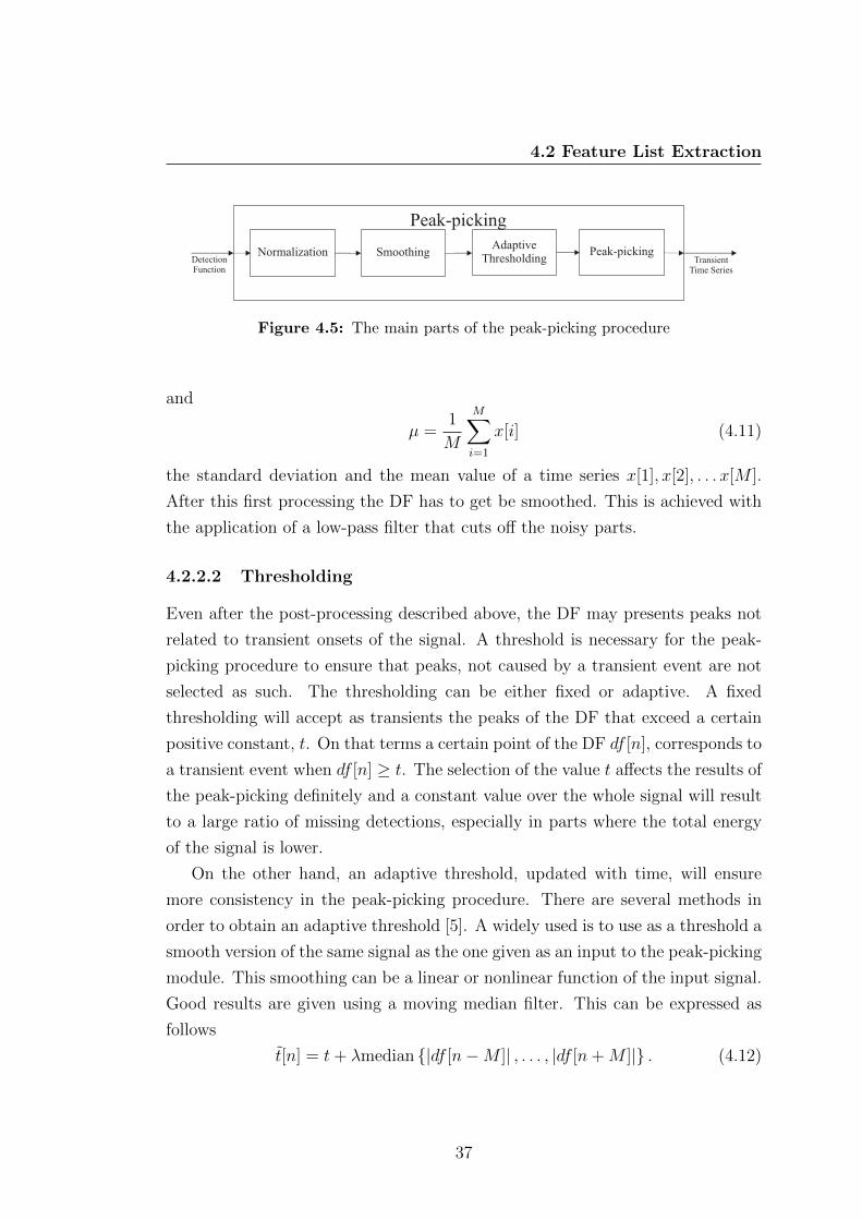
4.2 Feature List Extraction

Peak-picking

Normalization

Smoothing Peak-pickingAdaptive

ThresholdingDetectionFunction

Transient Time Series

Figure 4.5: The main parts of the peak-picking procedure

and

µ =1

M

M∑i=1

x[i] (4.11)

the standard deviation and the mean value of a time series x[1], x[2], . . . x[M ].

After this first processing the DF has to get be smoothed. This is achieved with

the application of a low-pass filter that cuts off the noisy parts.

4.2.2.2 Thresholding

Even after the post-processing described above, the DF may presents peaks not

related to transient onsets of the signal. A threshold is necessary for the peak-

picking procedure to ensure that peaks, not caused by a transient event are not

selected as such. The thresholding can be either fixed or adaptive. A fixed

thresholding will accept as transients the peaks of the DF that exceed a certain

positive constant, t. On that terms a certain point of the DF df [n], corresponds to

a transient event when df [n] ≥ t. The selection of the value t affects the results of

the peak-picking definitely and a constant value over the whole signal will result

to a large ratio of missing detections, especially in parts where the total energy

of the signal is lower.

On the other hand, an adaptive threshold, updated with time, will ensure

more consistency in the peak-picking procedure. There are several methods in

order to obtain an adaptive threshold [5]. A widely used is to use as a threshold a

smooth version of the same signal as the one given as an input to the peak-picking

module. This smoothing can be a linear or nonlinear function of the input signal.

Good results are given using a moving median filter. This can be expressed as

follows

t[n] = t+ λmedian {|df [n−M ]| , . . . , |df [n+M ]|} . (4.12)

37

4. PROPOSED METHOD

0 50 100 150 200 250 300 350 400 450 500−2

−1.5

−1

−0.5

0

0.5

1

Time

Am

plitu

de

0 50 100 150 200 250 300 350 400 450 500−0.5

0

0.5

1

Time

Am

plitu

de

Normalized DFAdaptive Threshold

DFSmoothed DF

Figure 4.6: The preprocessing of the DF before the peak-picking

where t is a predefined constant value, the threshold that is being adaptive ac-

cording to the median value of a block of 2M values of the DF.

4.2.2.3 Peak-picking

After obtaining a threshold for each value of the post-processed DF the remaining

task is as simple as choosing the local maxima of this function, that exceed the

defined threshold. These maxima are considered to correspond to the existence

of a new transient part in the initial audio signal.

A peak picking procedure, applied on the analysis frames (of length N) of the

smoothed and normalized signals dfk[n], produces a time series

tsk[n] =

{1 if dfk[n] demonstrates a peak here

0 otherwise(4.13)

During peak picking, the adaptive threshold calculated by equation (4.12) is used.

38

4.3 Pulse Induction

CombFilters

Resonators

...m [n]k

y [n]k,24

y [n]k,242

Figure 4.7: A bank of comb filters for frequency band k

4.2.3 Window application

The time series tsk[n] is then convolved with a Hanning window, in order to

produce the mask functions mk[n]. In that way, a strongly smoothed version

of the corresponding detection function is created, that however accentuates the

detected abrupt events. The above described processing for the creation of the

feature list combines the advantages of the use of an onset list with those methods

where the feature lists are obtained in a continuous manner.

4.3 Pulse Induction

The second part of the system, is where the periodicity analysis is carried out in

order to infer tempo from the list of features (i.e. mask functions) produced until

here. The periodicity analysis is done using a bank of Comb filters.

Each one of the mask functions, mk[n] is given as an input to a bank of Comb

filters. In that terms, for the analysis band k the following takes place:

yk,τ [n] = aτyk,τ [n− τ ] + (1− aτ )mk[n], (4.14)

for every τ ∈ T. The interval T ranges from 45 to 242 beats per minute (BMP). In

this interval the filter’s delay τ takes integer values. aτ corresponds to the filter’s

feedback gain and it is calculated as a = 0.5τT0 . The time during which the signal

should reach its half energy is T0. In this system T0 is equal to 4 seconds, a

time window small enough to quickly adapt to any tempo changes, but also long

enough to respond to a very slow tempo.

39

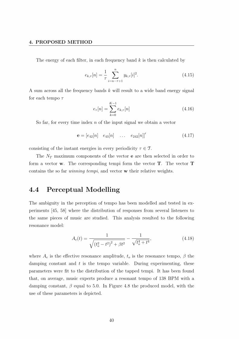
4. PROPOSED METHOD

The energy of each filter, in each frequency band k is then calculated by

ek,τ [n] =1

τ

n∑i=n−τ+1

yk,τ [i]2. (4.15)

A sum across all the frequency bands k will result to a wide band energy signal

for each tempo τ

eτ [n] =K−1∑k=0

ek,τ [n] (4.16)

So far, for every time index n of the input signal we obtain a vector

e = [e42[n] e43[n] . . . e242[n]]′ (4.17)

consisting of the instant energies in every periodicity τ ∈ T.

The NT maximum components of the vector e are then selected in order to

form a vector w. The corresponding tempi form the vector T. The vector T

contains the so far winning tempi, and vector w their relative weights.

4.4 Perceptual Modelling

The ambiguity in the perception of tempo has been modelled and tested in ex-

periments [45, 58] where the distribution of responses from several listeners to

the same pieces of music are studied. This analysis resulted to the following

resonance model:

Ae(t) =1√

(t2o − t2)2 + βt2

− 1√t4o + t4

, (4.18)

where Ae is the effective resonance amplitude, to is the resonance tempo, β the

damping constant and t is the tempo variable. During experimenting, these

parameters were fit to the distribution of the tapped tempi. It has been found

that, on average, music experts produce a resonant tempo of 138 BPM with a

damping constant, β equal to 5.0. In Figure 4.8 the produced model, with the

use of these parameters is depicted.

40

4.4 Perceptual Modelling

0 100 200 300 400 5000

0.02

0.04

0.06

Tempi (BPM)

Ampli

tude

Figure 4.8: The resonance model that was described in [45] to fit the distributions

of responses to several pieces of music.

We propose the use of this model in order to weight the results from the

periodicity analysis,

w′i = Ae(Ti)wi i ∈ [1, 2, . . . , NT ], (4.19)

where Ti the i-th value of vector T and wi the corresponding weight. After this

step, w′ contains the perceptually modified weights of the winning tempi in T.

The tempo estimation is therefore enhanced with perceptual information.

Systems that estimate periodicity patterns in a signal strongly respond to the

multiples and aliquots of any fundamental periodicity that appears in it. Likewise,

when it comes to human listeners, the more ambiguities in determining the tempo

appear due to the selection of multiples and divisors of the same tempo. In the

vector of winning tempi, T, also appear not only possible perceived tempi, but

also multiples and aliquots of them.

In order to discard some “false” estimations from T and decide which is

the perceived tempo in a group of tempi that have a common divisor, an extra

weighting step is introduced. During experimenting, it was found that increasing

the weights of each tempo that appears in T with a factor of the weight of its

multiples and divisors that also appear in T, has the following two desired effects:

a. Significant decrease in the (normalized) weights of tempi whose multiples

and aliquots are not present.

41

4. PROPOSED METHOD

b. Highly accurate decision on which is the true perceived tempo within a set

of tempi that have the same common divisor).

This factor was chosen experimentally as 0.3 for multiple periods and as 0.6 for

aliquots.

4.5 Conclusions

A method for estimating the tempo of polyphonic music signals has been proposed

in this Section. Four main parts comprise the final architecture:

1. Subspace Analysis The signal is separated in 16 frequency bands using

Gammatone subspace analysis. The algorithm treats each frequency band

separately, combining the results at the end.

2. Feature List Extraction Tempo induction cues are extracted and a signal

that describes the predominant rhythmic information of the input is created.

The cues considered in this study as tempo induction cues are the onsets of

transient events in the temporal representation of the signal. The detection

of these is done with the application of a peak picking procedure in the

output of an adaptive LPEF.

3. Pulse Induction The feature lists, produced in the previous step are given

as an input to a bank of Comb Filters Resonators. The energy of each

band of the feature list, in periodicities that vary from 42 to 242 BPM are

calculated there.

4. Perceptual Modelling The periodicities were feature lists have stronger

energy are considered “winning”. A model, inspired by the human percep-

tion of tempo is applied on these winning tempi in order to facilitate the

estimation of the final output.

42

Chapter 5

Evaluation and Results

The extraction of the feature lists, which are used for the tempo estimation task,

is considered as a critical part of the whole system. It is not however possible to

correctly evaluate this part as a separate unit, and obtain a quantitative measure

on how successful or accurate the feature list extraction is. Since the initial

motivation for the method that was developed, was the detection of transient

events in the input signal, the evaluation of this part is conducted in the context

of transient detection. More details on this part of the evaluation are given in

Section 5.1.

In the community of MIR, much effort has been dedicated to the automatic

detection of the tempo of music excerpts. However, until recently the field lacked

of systematic evaluation and proposed models did not present consistent quan-

titative measurements of their success rates. The reason for that was firstly the

diversity of different applications, as well as the diversity of input and output

data. Apart from that, evaluation datasets were usually private and of relatively

small size. The first systematic evaluation of tempo induction systems was per-

formed in 2004, as part of the International Conference on Music Information

Retrieval (ISMIR 2004). Based on the specifications introduced in this contest

and in a detailed report on it [26], the developed system is evaluated and com-

pared to the state-of-the-art in the field. The evaluation method and the results

are presented in Section 5.2.

43

5. EVALUATION AND RESULTS

5.1 Feature List Extraction

After designing the transient detection system, that forms the feature list used as

an input to the pulse induction block, an intermediate part of the evaluation was

conducted in order to ensure that this list is appropriate to be used as an input

to the next step of the system. The desired output of the feature list extraction

is a mask function that has non zero values around the detections of transient

events. Therefore, it is of importance to ensure the accuracy of the system in

detecting transient events.

5.1.1 Dataset and Ground-Truth

The first step of evaluating the transient detection method, is the creation of a

dataset that contains music signals and ground truth information for the transient

events that appear in each of these signals. In order to obtain the ground-truth

for a subjective evaluation of our results, a database that consists of hand-labelled

versions of the test samples should be created. This task of annotating the start-

ing point of every transient event within a music signal is time consuming and it

often results in ambiguous ground-truth labels [39]. Usually, the annotation of a

music file depends on the employed annotation method and the software that is

used, the listener-annotator and his understanding of musical events as well as

on the type of music and number of instruments. Since all these problems arise

in the procedure of annotating the starting points of musical events, it is critical

to provide a detailed method of how to realize this task. The next paragraphs

exhibit this detailed description of the whole annotation task.

Software used The software used for the labelling of the test samples was

Praat1, an open source software for acoustics, developed by Paul Boersma and

David Weenink at the Department of Phonetics in the University of Amsterdam.

Using Praat, the annotator can label a sample of sound using the interface shown

in Figure 5.1. As depicted there, the annotator can see in a single window both

the plot of the signal in time domain and the spectrogram of it. On the lower

1Available from http://www.fon.hum.uva.nl/praat/

44

5.1 Feature List Extraction

Figure 5.1: The Praat environment, used for the annotation of the sound test

files.

45

5. EVALUATION AND RESULTS

part of the window, the annotation area is visible. In this area, the annotator

can add, remove, and edit special boundaries that define the starting (or ending)

point of a new event. Each boundary can be assigned with a label that classifies

the adjacent event to a certain type of events.

Methods employed During the labelling of music events there are three widely

used methods that an annotator can employee in order to locate these events.

These namely are looking at the signal plot, looking at the signal spectrogram

and listening to signal slices [39]. In case of labelling transient events, looking

at the signal spectrogram is enough to roughly locate most of the corresponding

events. However, the poor time resolution of a spectrogram that provides suffi-

cient frequency resolution, does not allow the annotator to find the exact point

in time where the event takes places. The annotator has to use the other two

methods before applying the label. The ultimate judge should be listening to the

slice of the signal, around the located transient event and then, according to the

understanding of the event and the changing amplitude of signal plot, find the

exact starting point of the event.

Tolerance window In order to annotate the starting point of a transient event

within a music signal, a certain definition of this starting point is necessary.

However, as already described no such definition is currently available. The

exact point of the annotated event is completely up to the understanding of

the annotator. As an outcome it is almost impossible to obtain an annotation

completely unambiguous, and usually the maximum achieved precision is around

50ms [39]. Moreover, the annotator needs a very strict description of the events

that has to look for. During any multi-instrument music file, a big variety of

different events takes place; which of these events are of interest during annotation

completely depends on the nature of the developed algorithm. In our case, the

events of interest are the starting points of transient events. It is rather easy to

locate such events when they are caused by the onset of a percussive note, but

when more than one instruments are involved in a single file, the task gets more

and more complicated.

46

5.1 Feature List Extraction

5.1.2 Term definitions and evaluation measures

After the creation of the ground-truth data set, we are ready to commence the

actual evaluation procedure. However, it is necessary to define the correct eval-

uation measures which are going to give the final score of the system and prove

either its success or its failure. The measures that are used are widely recognised

as appropriate measures for any kind of information retrieval tasks. MIREX [1]

contest also describes similar measures for the evaluation of submitted algorithms

in the field of MIR.

During objective evaluation, the detected events are compared with the ground-

truth ones. For a given ground-truth event, if there is a detection within a tol-

erance window, it is considered as a correct detection, Tcd. If not, it is a false

negative, Tfn. Every detected event, outside the tolerance window is counted as

a false positive, Tfp. A subset of Tfn events are the merged events, Tm, where

one detection takes place for two ground-truth events. Finally, doubled events,

Td, are those detections where two events are mapped to the same ground-truth

event. Td is a subset of Tfp.

Two widely used statistical classifications defined for information retrieval are

the precision, p, and recall, r. Precision is defined as

p =Tcd

Tcd + Tfp(5.1)

and refers to the exactness or fidelity of the result. On the other hand, recall can

be seen as a measure of completeness and is defined as

r =Tcd

Tcd + Tfn. (5.2)

Combining these two measures, we can obtain the F-measure, that is the weighted

harmonic mean of precision and recall. The F-measure is a widely used measure

[1, 13], that provides an accuracy value for the output of an information retrieval

algorithm. It can be expressed as

F =2pr

p+ r. (5.3)

In addition to F-measure, common evalutation measures for onset detection, that

can be applied to the task of the developed algorithm are the folowing:

47

5. EVALUATION AND RESULTS

Argument ID Argument Description

inArg01 winLen The length of the transients modelling window

inArg02 winType The shape of the transients modelling window

inArg03 ppThres The static threshold for the peak picking algo-

rithm

inArg04 intTime The minimum interval time between two events

so that they may be considered different tran-

sients

inArg05 dfType A flag that defines whether the results should be

obtained with wideband or band-wise processing

inArg06 wFunc The weighting function to be used for weighting

each analysis sub-band

Table 5.1: The defined input arguments for the Transient Detection and Separa-

tion system.

1. False positive Rate: fpr =Tfp

Tcd+Tfp,

2. Doubled events Rate in Tfp: dr = TdTfp

and

3. Merged events Rate in Tfn: mr = TmTfn

.

5.1.3 Results

The modules that conduct transient detection and modelling of transient events

in a set of mask functions, can be adjusted in a high degree, by modifying a

specific set of input arguments. Any evaluation results for the final tool highly

depend on the selection of a specific argument set. Table 5.1 presents an overview

of all these input arguments, along with a short description of their function.

The understanding of the way that each of them affects the final results is quite

important as this will allow to obtain a subset of input arguments which can be

tested before deciding the optimum set of input arguments to be used for (a)

obtaining the final results and (b) extracting the most accurate possible feature

list.

48

5.1 Feature List Extraction

• Argument inArg01: winLen After the execution of the peak picking

algorithm and the generation of a transient time series, mask windows are

placed around each detected event. The length of the used window is a

quite important variable. The idea is that this length will approach the

length of a transient onset as much as possible.

• Argument inArg02: winType Apart from the length of the separation

window, another quite critical argument is the shape of this window. In

order to model transient events, the window has to follow a very generalized

envelope of such events. Figure 5.2 illustrates three of the windows that

were considered to be used in order to model a transient event. Based on

the intuitive description of transients events, the selected mask function

should follow the evolution of these events, having the attack and decay

phase. These parts are better modelled from the BBT window. However,

as this window is thinner in the higher values and wider in the lower, it is

quite important to correctly place it around a detected transient. On the

other hand, using a window that also allows a wide range of high values

to pass through, makes the modelling robust in slight differences in timing.

Based on that, windows like the Hanning and the Gamma were also used

and tested.

• Arguments inArg03: ppThres & inArg04: intTime The peak pick-

ing procedure used in the detection algorithm is the part that is affected

the most from different argument values. When local maxima have to be

detected on an input function using a peak picking procedure, it is critical

to correctly define the threshold and the minimum interval time between

two local peaks. Giving a very big value as a threshold, important events

may be discarded as non transient while a very low threshold would result

to the opposite, that is considering a big set of irrelevant events as tran-

sient information. As far as the time interval between selected peaks is

concerned, it is also an important argument. A very small interval would

result to several detections for a single event while the opposite, that is a

very big time interval would result to a bigger false negative value since

each detected event would act as a masker for the following events.

49

5. EVALUATION AND RESULTS

0 0.01 0.02 0.03 0.04 0.050

0.2

0.4

0.6

0.8

1

Time

Am

plitu

de

HanninngGammaBBT

Figure 5.2: The predefined separation windows

• Argument inArg05: dfType As described in previous sections, the de-

signed system is able to provide transient information either in a wide band

or a narrow band representation. It is important to note here, that since

the wideband results are not obtained via a simple adding across the several

frequency bands, it increases the efficiency of the detection module but also

the processing demands of it. The activation of this extra processing can

be controlled by this argument.

• Argument inArg06: wFunc In case the extra processing for producing

a wide band detection function is enabled, the way that the information is

combined can be partially controlled by this parameter. Detections from

different frequency bands affect the corresponding wide band detections

in different ways, is formulated through this argument that describes the

weighting method for each sub space frequency band.

Determining Optimum Set of Arguments A final step is missing before

obtaining the final scores of the transient detection algorithm. This is to obtain

50

5.2 Tempo Estimation

Argument ID Argument Values

inArg01 winLen 0.05, 0.1 & 0.2 sec

inArg02 winType Hanning

inArg03 ppThres 0.05 - 0.4 sec of the maximum am-

plitude

inArg04 intTime 0.02, 0.05 & 0.2 sec

inArg05 dfType wide band

inArg06 wFunc no

Table 5.2: The selected subset of arguments for which testing took place.

the optimum set of arguments. To do so, an exhaustive testing of several argument

sets took place. The set that optimized the average F-score of the system over

the dataset was selected to be the one used as the default.

In Table 5.2 the selected sets of arguments during this testing are presented.

All the possible combinations of the different arguments formed more than 70 test

cases. In Figure 5.3 the average F-score that was obtained from the various test

cases, over all the test files, is illustrated. Based on this figure, the combination

that was chosen is the one that corresponds to the 5th test case.

Final Results for the Optimum Argument Set Using this set of arguments,

Figure 5.4 illustrates the F-score of the system for 6 test files. Separately results

for all the evaluation measures defined earlier are given in Table 5.5.

5.2 Tempo Estimation

5.2.1 Datasets and Evaluation Measures

The developed system is evaluated using the measures proposed in [26]. The two

measures defined are Accuracy 1 and Accuracy 2, corresponding to the percentage

of tempo estimates within 4% of the ground truth data. For the calculation of

Accuracy 2 integer multiplications and divisions of the ground-truth tempo are

also considered to be correct estimates. This is motivated by the fact that the

51

5. EVALUATION AND RESULTS

0 10 20 30 40 50 60 70 800.55

0.6

0.65

0.7

0.75

0.8

0.85

0.9

Test Case

F−

sco

res

Figure 5.3: The average F-scores that the system achieved for the different test

cases.

File ID F fpr dr mr

f01 0.9 0.18 0 0

f02 0.63 0.53 0 0

f03 1 0 0 0

f04 0.83 0 0 0.05

f05 0.92 0.14 0.08 0

f06 0.73 0.42 0 0

Table 5.3: The results per file for the optimum set of arguments

52

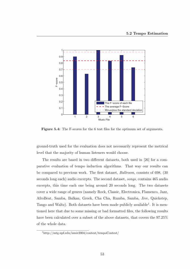
5.2 Tempo Estimation

1 2 3 4 5 60

0.1

0.2

0.3

0.4

0.5

0.6

0.7

0.8

0.9

1

Music File

F−

score

The F−score of each file

The average F−Score

Minus/plus the standard deviation

Figure 5.4: The F-scores for the 6 test files for the optimum set of arguments.

ground-truth used for the evaluation does not necessarily represent the metrical

level that the majority of human listeners would choose.

The results are based in two different datasets, both used in [26] for a com-

parative evaluation of tempo induction algorithms. That way our results can

be compared to previous work. The first dataset, Ballroom, consists of 698, (30

seconds long each) audio excerpts. The second dataset, songs, contains 465 audio

excerpts, this time each one being around 20 seconds long. The two datasets

cover a wide range of genres (namely Rock, Classic, Electronica, Flamenco, Jazz,

AfroBeat, Samba, Balkan, Greek, Cha Cha, Rumba, Samba, Jive, Quickstep,

Tango and Waltz). Both datasets have been made publicly available1. It is men-

tioned here that due to some missing or bad formatted files, the following results

have been calculated over a subset of the above datasets, that covers the 97.25%

of the whole data.

1http://mtg.upf.edu/ismir2004/contest/tempoContest/

53

5. EVALUATION AND RESULTS

Winning

TempiT1 T2 T3 T4 T5

Accuracy

1

(%)

38.40 28.22 6.02 1.72 2.44

Accuracy

1

CDF (%)

38.40 66.62 72.64 74.36 76.80

Table 5.4: The Accuracy 1 of the algorithm for the estimation of the winning

tempi

5.2.2 Results

The first phase of the evaluation procedure was to check the accuracy of the

algorithm in defining the vector of the winning tempi, T, i.e. before applying the

perceptual modelling. The winning tempi in the vector are placed in descending

order, based on their weight. In Table 5.4, the results on the Ballroom dataset

are illustrated. In the first row, the Accuracy 1 of the algorithm in each index of

the winning tempi is shown. The next row, presents the cumulative results up to

each index of the vector T. As depicted in this table, the algorithm has a success

rate of 76.8% in estimating the correct tempo in the first 5 estimations.

The perceptual model at the end was inspired by this ambiguity in the results.

Although the algorithm is quite accurate in detecting the right periodicity from

a music excerpt, it has a relatively low percentage (38.4%) to do so in the first

guess (i.e. the tempo with the higher energy). Until this point, only low-level

music features have been used. The encoding of higher level knowledge on tempo

perception in the model could be useful in choosing the right index of the winning

tempi vector as the final estimation.

Indeed, the last step of the system achieves this task. The perceptual method

is applied to the output, improving significantly the results of the algorithm. The

results for both datasets, for the two evaluation metrics can be seen in Table 5.5.

In the first row the results of the two datasets are presented, for both measures

54

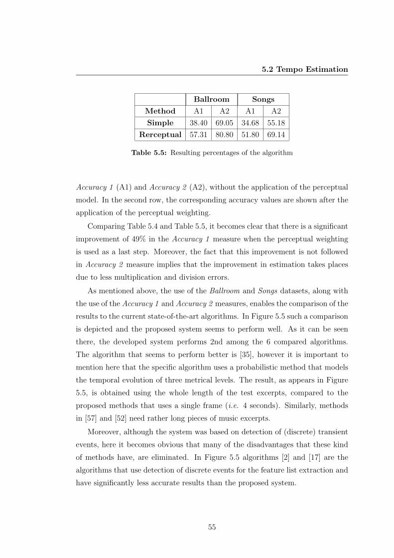
5.2 Tempo Estimation

Ballroom Songs

Method A1 A2 A1 A2

Simple 38.40 69.05 34.68 55.18

Rerceptual 57.31 80.80 51.80 69.14

Table 5.5: Resulting percentages of the algorithm

Accuracy 1 (A1) and Accuracy 2 (A2), without the application of the perceptual

model. In the second row, the corresponding accuracy values are shown after the

application of the perceptual weighting.

Comparing Table 5.4 and Table 5.5, it becomes clear that there is a significant

improvement of 49% in the Accuracy 1 measure when the perceptual weighting

is used as a last step. Moreover, the fact that this improvement is not followed

in Accuracy 2 measure implies that the improvement in estimation takes places

due to less multiplication and division errors.

As mentioned above, the use of the Ballroom and Songs datasets, along with

the use of the Accuracy 1 and Accuracy 2 measures, enables the comparison of the

results to the current state-of-the-art algorithms. In Figure 5.5 such a comparison

is depicted and the proposed system seems to perform well. As it can be seen

there, the developed system performs 2nd among the 6 compared algorithms.

The algorithm that seems to perform better is [35], however it is important to

mention here that the specific algorithm uses a probabilistic method that models

the temporal evolution of three metrical levels. The result, as appears in Figure

5.5, is obtained using the whole length of the test excerpts, compared to the

proposed methods that uses a single frame (i.e. 4 seconds). Similarly, methods

in [57] and [52] need rather long pieces of music excerpts.

Moreover, although the system was based on detection of (discrete) transient

events, here it becomes obvious that many of the disadvantages that these kind

of methods have, are eliminated. In Figure 5.5 algorithms [2] and [17] are the

algorithms that use detection of discrete events for the feature list extraction and

have significantly less accurate results than the proposed system.

55

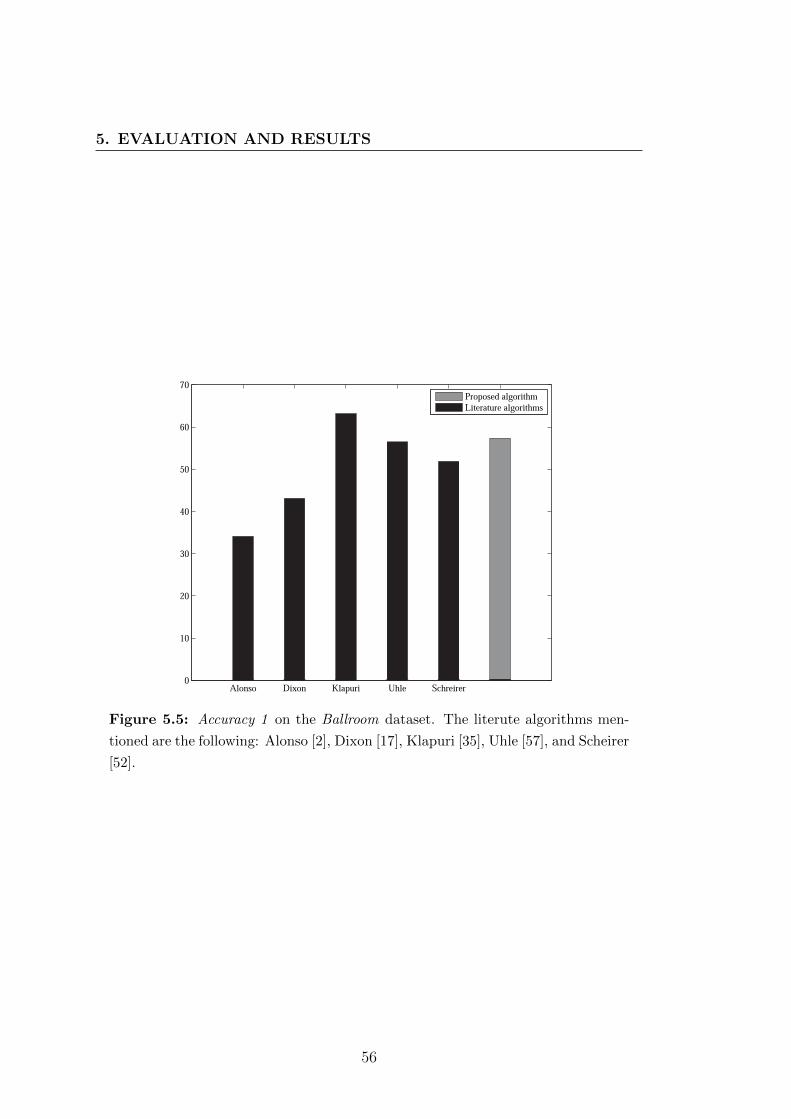
5. EVALUATION AND RESULTS

Alonso Dixon Klapuri Uhle Schreirer0

10

20

30

40

50

60

70Proposed algorithmLiterature algorithms

Figure 5.5: Accuracy 1 on the Ballroom dataset. The literute algorithms men-

tioned are the following: Alonso [2], Dixon [17], Klapuri [35], Uhle [57], and Scheirer

[52].

56

5.3 Conclusions

5.3 Conclusions

The evaluation of the developed system, conducted in two stages, was presented

in this chapter. During the first stage, the feature list extraction method was

evaluated on its success to correctly detect transient events, which are considered

to be the tempo induction cues. Since the database used for this stage of evalua-

tion was a very small database created only for this task, no comparison to other

literature algorithm could be presented. However, as the goal of this stage was to

have an intermediate understanding of the system accuracy, such a comparison

was considered to be beyond the scope of this thesis.

The final, and more critical stage of the evaluation, was that of the accuracy

in estimating the tempo of a given music excerpt. The results, obtained on a

widely used dataset, could be compared to the current state-of-the-art on the field.

This comparison showed that the algorithm operates well. Further improvements

to the proposed method though are envisioned and these are discussed in the

following chapter.

57

5. EVALUATION AND RESULTS

58

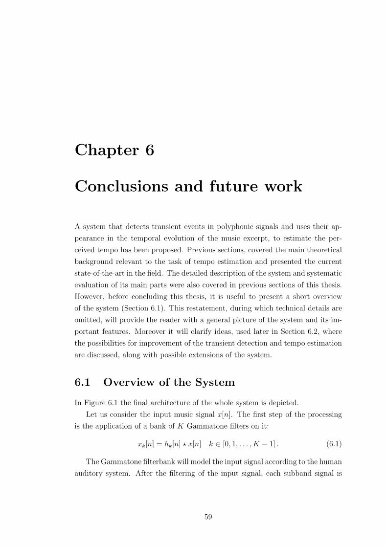
Chapter 6

Conclusions and future work

A system that detects transient events in polyphonic signals and uses their ap-

pearance in the temporal evolution of the music excerpt, to estimate the per-

ceived tempo has been proposed. Previous sections, covered the main theoretical

background relevant to the task of tempo estimation and presented the current

state-of-the-art in the field. The detailed description of the system and systematic

evaluation of its main parts were also covered in previous sections of this thesis.

However, before concluding this thesis, it is useful to present a short overview

of the system (Section 6.1). This restatement, during which technical details are

omitted, will provide the reader with a general picture of the system and its im-

portant features. Moreover it will clarify ideas, used later in Section 6.2, where

the possibilities for improvement of the transient detection and tempo estimation

are discussed, along with possible extensions of the system.

6.1 Overview of the System

In Figure 6.1 the final architecture of the whole system is depicted.

Let us consider the input music signal x[n]. The first step of the processing

is the application of a bank of K Gammatone filters on it:

xk[n] = hk[n] ? x[n] k ∈ [0, 1, . . . , K − 1] . (6.1)

The Gammatone filterbank will model the input signal according to the human

auditory system. After the filtering of the input signal, each subband signal is

59

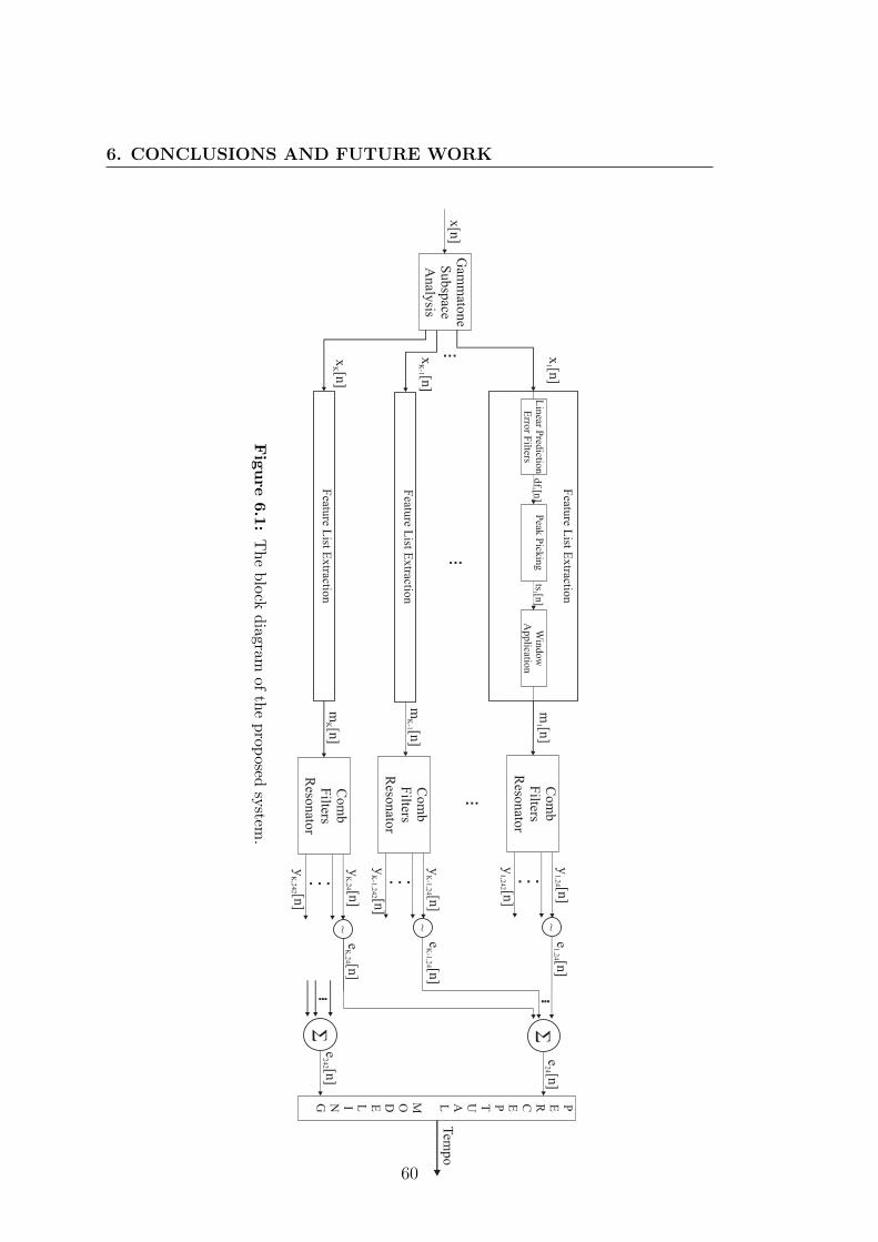
6. CONCLUSIONS AND FUTURE WORK

Feature L

ist Extraction

Linear P

redictio

n

Error F

iltersP

eak P

ickingW

indow

Application

x[n]

1m

[n]1

df

[n]

1ts

[n]1

Feature L

ist Extraction

Feature L

ist Extraction

...

Com

bF

iltersR

esonato

r

...

y[n]

1,24

y[n

]1,242

m[n]

K

Co

mb

Filters

Reson

ator

...

y[n]

K,24

y[n]

K,242

...

ΣΣ

PERCEPTUALMODELING

Tem

po

e[n]

1,24e

[n]24

e[n

]242

Gam

matone

Su

bspace A

nalysis

x[n]

...

Com

bF

iltersR

esonato

r

...

y[n]

K-1,24

y[n]

K-1,242

m[n

]K

-1

x[n]

K

x[n

]K

-1

~

e[n]

K-1,24

~

e[n]

K,24

~

......

Figure

6.1:

Th

eb

lock

diagram

ofth

ep

roposed

system

.

60

6.1 Overview of the System

decimated K times as follows

xk[n] = xk[Kn]. (6.2)

The xk[n] signals are then given as an input to the bank of adaptive LPEFs,

forming the detection function, which is the prediction error of an adaptive linear

predictive algorithm. The algorithm is based on estimating the LPC coefficients

of the initial M values of the N long frame, and adapting this coefficients using

the Least Mean Square (LMS) algorithm. The output of the adaptive LPEF,

dfk[n] is a residual signal that presents high values when abrupt events take place

in the temporal evolution of the signal.

The dfk[n] signals are then smoothed and normalized and a peak picking

procedure, is applied on them producing a time series

tsk[n] =

{1 if dfk[n] demonstrates a peak here

0 otherwise(6.3)

During peak picking, an adaptive threshold, calculated by the sum of a predefined,

static threshold and a moving median filter is used.

The time series tsk[n] are then convolved with a Hanning window, in order

to produce the mask functions mk[n]. In that way, a strongly smoothed version

of the corresponding detection function is created, that however accentuates the

detected abrupt events.

In the second part of the system, tempo induction is carried out with the use

of a comb filter resonator for each frequency band k. The energy of the output

of each filter, in each frequency band k, is calculated and used in

eτ [n] =K∑k=1

ek,τ [n], (6.4)

where the sum across all the frequency bands k results to a wide band energy

signal for each tempo τ .

The maximum components of the vector e are then selected in order to form

a vector w. The corresponding tempi form the vector T. The vector T contains

the so far winning tempi, and vector w their relative weights.

61

6. CONCLUSIONS AND FUTURE WORK

The next and final step is the application of the resonance model and the

perceptual weighting. The results from the periodicity analysis are then weighted

with the perceptual model Ae(t) and factor of the weights of their multiples and

aliquots. The maximum weighted tempo is given to the output and considered

to be the estimated tempo for the input signal x[n]

6.2 Future Work

A new method to estimate the tempo of musical signals, based on detection of

transient events, was presented. The evaluation of this method was conducted

using popular datasets for the tempo estimation task along with previously de-

fined evaluation measures. Although at an early stage, the algorithm seems to

operate very well in comparison to the state-of-the-art, using only a single frame

(4 seconds long) for calculating the result. The part of extracting the feature

list, based on a transient detection technique, was though evaluated in a much

narrower range of dataset. A more systematic evaluation of this part, separately

could give use an even better insight on how this part can be improved.

As mentioned, the above described results are obtained from a single frame of

the input signal. An application of the algorithm on the whole signal, and then

the computation of a median or average tempo estimate did not seem to yield

a significant improvement. However, the implementation of a voting mechanism

could improve the overall tempo estimation of a piece. In such an extension an

extra assumption has to be made, i.e. that the tempo of the piece does not

present any variations throughout the song.

The use of LPEFs introduced by this work, seems to work well in the task of

extracting tempo estimation features (i.e.transient detection). However, it was

observed during experimenting, that the final results and success rates, of both the

transient detection module and the tempo estimation system, are sensitive to the

the set of parameters used by the feature list extraction part (LPC order, peak

picking static threshold). A detailed examination of the results from different

parameter sets and the determination of an optimum set may further improve

the accuracy of the whole system.

62

6.2 Future Work

Until now, the existing knowledge on the perceptual event that leads to the

well known action of foot-tapping, has not been extensively used for a systematic

way of estimating perceived tempo. This study indicates that taking advantage

of auditory modelling tools can significantly improve the performance of a tempo

estimation algorithm.

63

6. CONCLUSIONS AND FUTURE WORK

64

References

[1] Music information retrieval evaluation exchange: 2006: Audio onset de-

tection: Evaluation procedures. http://www.music-ir.org/mirex/wiki/

2006:Audio_Onset_Detection. 47

[2] M. Alonso, B. David, and G. Richard. Tempo and beat estimation of

musical signals. In Proceedings of the 5th International Conference on Music

Information Retrieval, Barcelona, Spain, 2004. xii, 17, 55, 56

[3] D. Barry, D. Fitzgerald, E. Coyle, and B. Lawlor. Drum source

separation using percussive feature detection and spectral modulation. In

Proceedings of the Irish Signals and Systems Conference, 2005. 22

[4] M. Basseville and I. V. Nikiforov. Detection of Abrupt Changes -

Theory and Applications. Prentice-Hall, 1993. 24

[5] J. B. Bello, L. Daudet, S. Abdallah, C. Duxbury, M. Davies,

and M. B. Sandler. A tutorial on onset detection in music signals. IEEE

Transactions on Speech and Audio Processing, 13(5):1035–1047, September

2005. xi, 19, 20, 37

[6] J. P. Bello, C. Duxbury, M. Davies, and M. Sandler. On the use of

phase and energy for musical onset detection in the complex domain. IEEE

Signal Processing Lett., 11(6):553–556, 2004. 23

[7] J. P. Bello and M. Sandler. Phase-based note onset detection for music

signals. In Proceedings of the IEEE International Conference on Acoustics,

Speech, and Signal Processing (ICASSP-03), pages 49–52, 2003. 23

65

REFERENCES

[8] T. L. Blum, D. F. Keislar, J. A. Wheaton, and E. H. Wold.

Method and article of manufacture for content-based analysis, storage, re-

trieval, and segmentation of audio information, June 1999. 18

[9] A. S. Bregman. Computational auditory scene analysis. chapter Psy-

chological data and computational ASA, pages 1–12. L. Erlbaum Associates

Inc., 1998. 29

[10] J. C. Brown. Determination of the meter of musical scores by autocorre-

lation. Journal of Acoustical Society of America, 94(4):1953–1957, 1993. 16,

17, 18

[11] J. Chowning, L. Rush, M. R. Bernard, C. Chris, W. A. Schloss,

and O. S. Julius. Intelligent systems for the analysis of digitized acous-

tic signals, final report. Technical Report STAN-M-15, Stanford University

Department of Music, 1984. 16

[12] R. B. Dannenberg and B. Mont-Reynaud. Following an Improvisation

in Real Time, pages 241–248. International Computer Music Association,

1987. 18

[13] M. E. P. Davies, N. Degara, and M. D. Plumbley. Evaluation

methods for musical audio beat tracking algorithms. Technical report, Center

for Digital Music, Queen Mary University of London, 2009. 47

[14] M. P. E. Davies and M. D. Plumbley. Context-dependent beat tracking

of musical audio. Audio, Speech, and Language Processing, IEEE Transac-

tions on, 15(3):1009–1020, March 2007. 17

[15] S. Dixon. Automatic extraction of tempo and beat from expressive perfor-

mances. Journal of New Music Research, 30:39–58, 2001. 17

[16] S. Dixon and E. Cambouropoulos. Beat tracking with musical knowl-

edge. In Proceedings of the 14th European Conference on Artificial Intelli-

gence, pages 626–630, 2000. 16, 17

66

REFERENCES

[17] S. Dixon, E. Pampalk, and Widmer G. Classification of dance music

by periodicity patterns. In Proceedings of the International Conference on

Music Information Retrieval, pages 159–165, 2003. xii, 17, 18, 55, 56

[18] J. Durbin. The fitting of time series models. Rev. Inst. Int. Stat., 28:233–

243, 1960. 33

[19] C. Duxbury, J. P. Bello, M. Davies, and M. Sandler. A combined

phase and amplitude based approach to onset detection for audio segmen-

tation. In Proceedings of the 4th European Workshop on Image Analysis for

Multimedia Interactive Services (WIAMIS-03), pages 275–280, 2003. 23

[20] C. Duxbury, M. Sandler, and M. Davies. A hybrid approach to mu-

sical note onset detection. In Proceedings of the Digital Audio Effects Con-

ference (DAFX-02), pages 33–38, 2002. 23, 25

[21] J. Flanagan. Models for approximating basilar membrane displacement.

Journal Acoustic Society of America, 32:937, 1960. 8

[22] B. R. Glasberg and B. C. Moore. Derivation of auditory filter shapes

from notched-noise data. Hearing Research, pages 103–108, 1990. 10

[23] M. Goto. An audio-based real-time beat tracking system for music with or

without drum-sounds. 2001. 17, 18

[24] M. Goto and Y. Muraoka. Beat tracking based on multiple-agent ar-

chitecture: a real-time beat tracking system for audio signals. In Proceedings

of the 2nd Internationl Conference on Multiagent Systems, pages 103–110,

1996. 21, 23

[25] F. Gouyon and S. Dixon. A review of automatic rhythm description

systems. Computer Music Journal, 29(1):34–54, 2005. 16

[26] F. Gouyon, A. Klapuri, S. Dixon, M. Alonso, G. Tzanetakis,

C. Uhle, and P. Cano. An experimental comparison of audio tempo in-

duction algorithms. Audio, Speech, and Language Processing, IEEE Trans-

actions on, 14(5):1832–1844, sept. 2006. 16, 43, 51, 53

67

REFERENCES

[27] F. Gouyon, F. Pachet, and O. Delerue. On the use of zero-crossing

rate for an application of classification of percussive sounds. In Proceedings

of the COST G-6 Conference on Digital Audio Effects (DAFX-00, 2000. 17,

18

[28] S. Haykin. Adaptive filter theory. Prentice Hall, 1995. 33, 35

[29] A. Holzapfel and Y. Stylianou. Beat tracking using group delay based

onset detection. In Proceedings of the International Conference on Music

Information Retrieval, 2008. 23

[30] T. Irino. An optimal auditory filter. Proceedings of the IEEE Workshop

on Applications of Signal Processing to Audio and Acoustics, pages 198–201,

1995. 8

[31] T. Jehan. Musical Signal Parameter Estimation. Master’s thesis, Univercity

of California, Berkeley, CA, 1997. 24

[32] P. I. M. Johanesma. The pre-response stimulus ensemble of neurons in

the cochlear nucleus. In Proceedings of the Symposium on Hearing Theory,

pages 58–69, 1972. 8

[33] I. Kauppinen. Methods for detecting impulsive noise in speech and audio

signals. In Proceedings of the 14th International Conference on Digital Signal

Processing (DSP2002), pages 967–970, 2002. 25

[34] A. Klapuri. Sound onset detection by applying psychoacoustic knowledge.

In Proc. IEEE ICASSP’1999, pages 3089–3092, 1999. 22, 23

[35] A. P. Klapuri, A. J. Eronen, and J. T. Astola. Analysis of the meter

of acoustic musical signals. Audio, Speech and Language Processing, IEEE

Transactions on, 14(1), 2006. xii, 12, 17, 18, 55, 56

[36] E. W. Large and J. F. Kolen. Resonance and the perception of musical

meter. Connection Science, 6(1):177–208, 1994. 18

68

REFERENCES

[37] J. H. Lee and Downie J. S. Survey of music information needs, uses, and

seeking behaviours: Preliminary findings. In Proceedings of the International

Conference on Music Information Retrieval, pages 441–446, 2004. 1

[38] F. Lerdahl and R. Jackendoff. A Generative Theory of Tonal Music.

The MIT Press, 1983. 13

[39] P. Leveau, L. Daudet, and G. Richard. Methodology and tools for the

evaluation of automatic onset detection algorithms in music. In Proceecings

of the International Symposium on Music Information Retrieval, pages 72–

75, 2004. 44, 46

[40] S. Levine. Audio Representations for Data Compression and Compressed

Domain Processing. PhD thesis, Stanford University, Stanford, CA, 1998.

22, 23

[41] N. Levinson. The wiener rms error criterion in filter design and prediction.

J. Math. Phys., 25:261–278, 1947. 33

[42] C. Longuet-Higgins and C. S. Lee. The perception of musical rhythms.

Perception, 11:115–128, 1982. 16, 17, 18

[43] P. Marsi. Computer Modelling of Sound for Transformation and Synthesis

of Musical Signal. PhD thesis, University of Bristol, Bristol, UK, 1996. 23

[44] R. J. McAulay and T. F. Quatieri. Speech analysis/synthesis based on

a sinusoidal representation. IEEE Transactions on Acoustics, Speech, and

Signal Processing, 34(4):744–754, August 1986. 22

[45] D. Moelants and M. F. McKinney. Tempo perception and musical

content: What makes a piece fast, slow or temporally ambiguous. In Proceed-

ings of the 8th International Conference on Music Perception and Cognition,

2004. xii, 30, 40, 41

[46] B. Moore, B. Glasberg, and T. Bear. A model for the prediction

of thresholds, loudness and partial loudness. Journal of Audio Engineering

Society, 45(4):224–239, 1997. 23, 25

69

REFERENCES

[47] R. Parncutt. A perceptual model of pulse salience and metrical accent in

musical rhythms. Music Perception, 11(4):409–464, 1994. 17

[48] R. D. Patterson, K. Robinson, J. Holdsworth, D. McKeown,

C. Zhang, and Allerhand M. Complex sounds and auditory images.

pages 123–177, 1992. 8

[49] C. Raphael. A hybrid graphical model for rhythmic parsing. Artificial

Intelligence, 137:217–238, May 2002. 16

[50] X. Rodet and F. Jaillet. Detection and modelling of fast attack tran-

sients. In Proceedings of the International Computer Music Conference,

pages 30–33, 2001. 23

[51] E. Scheirer and M. Slaney. Construction and evaluation of a ro-

bust multifeature speech/music discriminator. In Proceedings of the 1997

IEEE International Conference on Acoustics, Speech, and Signal Processing

(ICASSP ’97), pages 1331–, 1997. 18

[52] E. D. Scheirer. Tempo and beat analysis of acoustic musical signals.

Acoustical Society of America, 103(1):588–601, January 1998. xii, 17, 18,

21, 55, 56

[53] W. A. Schloss. On the Automatic Transcription of Percussive Music -

From Acoustic Signal to High-Level Analysis. Master’s thesis, Stanford Uni-

versity, Stanford, CA, 1985. 16

[54] L. Smith and P. Kovesi. A continuous time-frequency approach to rep-

resenting rhythmic strata. In In Proc. 4th Int. Conf. on Music Perception

and Cognition, pages 197–202, 1996. 18

[55] H. Thornburg and F. Gouyon. A flexible analysis-synthesis method for

transients. In Proceedings of the International Computer Music Conference,

pages 400–403, 2000. 24

[56] G. Tzanetakis, G. Essl, and P. Cook. Human perception and com-

puter extraction of musical beat strength. In Proceedings DAFx-02, pages

257–261, 2002. 18

70

REFERENCES

[57] C. Uhle, J. Rohden, M. Cremer, and J. Herre. Low complexity

musical meter estimation from polyphonic music. In Audio Engineering So-

ciety Conference: 25th International Conference: Metadata for Audio, pages

63–68, New York, 2004. xii, 18, 55, 56

[58] L. Van Noorder and D. Moelants. Resonance and the perception of

musical meter. Journal of New Music Research, 28(1):43–66, 1999. 40

[59] T. S. Verma and T. Y. H. Meng. An analysis/synthesis tool for transient

signals that allows a flexible sines+transients+noise model for audio. In Proc.

IEEE ICASSP’1998, pages 3573–3576, 1998. 22

[60] Y. Wang and M. Vilermo. A compressed domain beat detector using

mp3 audio bitstreams. In Proceedings of the ninth ACM international con-

ference on Multimedia, pages 194–202, 2001. 16

71