transient heat conduction from · pdf filetransient heat conduction from spheroids rajai...

TRANSIENT HEAT CONDUCTION FROM SPHEROIDS

Rajai Alassar, Mohammed Abushosha and Mohammed El-GebeilyDepartment of Mathematics and Statistics, King Fahd University of Petroleum & Minerals, Dhahran, Saudi Arabia

E-mail: [email protected]

Received August 2013 Accepted March 2014No. 13-CSME-153, E.I.C. Accession 3611

ABSTRACTWe study the unsteady heat conduction from a spheroid (prolate or oblate) initially heated and then leftto cool in an unbounded medium of constant temperature. We present two solutions of the problem. Thefirst makes use of the spheroidal wave functions as basis. The second, which is numerical, is obtained byexpanding the dimensionless temperature in terms of Legendre functions and then solving the resulting setof differential equations in the radial direction using an implicit finite difference scheme. The two solutionsare further verified by comparing them to the limiting case of a sphere. We study the effect of the axis ratioon the time development of temperature inside the spheroid and the heat flux across the surface.

Keywords: spheroid; prolate; oblate; transient; heat conduction.

LE TRANSFERT TRANSITOIRE DE LA CHALEUR D’UN SPHEROIDE

RÉSUMÉNous étudions le transfert instationnaire de la chaleur d’un sphéroïde (allongé ou aplati) initialement chaufféet refroidie dans un environnement sans bornes à la température fixe. Nous présentons deux solutions de ceproblème. La première solution fait l’usage des fonctions d’ondes sphéroïdales en tant que base. La se-conde solution, qui est numérique, est obtenue en deux étapes. Après avoir développé la température sansdimension en termes des fonctions de Legendre, nous résolvons l’ensemble des équations différentiellesconsistant des parties radiales en utilisant un schéma implicite aux différences finies. En outre, nous compa-rons les deux solutions dans le cas d’une sphère. Nous étudions l’effet du rapport axial sur le développementen temps de la température à l’intérieur du sphéroïde et sur le flux de chaleur à travers de la surface.

Mots-clés : sphéroïde; allongé; aplati; transitoire; transfert de la chaleur.

Transactions of the Canadian Society for Mechanical Engineering, Vol. 38, No. 3, 2014 373

NOMENCLATURE

T0 initial uniform temperature of spheroidTf constant temperature of the surrounding mediuma length of semi-major axisb length of semi-minor axisη angular variable of spheroidal coordinate systemsξ radial variable of spheroidal coordinate systemsφ azimuthal variable of spheroidal coordinate systemshη angular scale factor of spheroidal coordinate systemshξ radial scale factor of spheroidal coordinate systemshφ azimuthal scale factor of spheroidal coordinate systemsc focal distanceξ0 parameter that defines the surface (ξ0 = tanh−1(b/a))T temperatureα thermal diffusivityt timeU dimensionless temperatureU average dimensionless temperatureτ dimensionless time` length scaleas radius of sphereλ time separation constantβ angular-radial variables separation constantq heat fluxNu local heat transfer numberNu average heat transfer numberµ transformation variable (µ = cosη)γ transformation variable (γ = coshξ ,γ0 = coshξ0)

R(1)mn radial wave functions of the first kind

R(2)mn radial wave functions of the second kind

S(1)mn angular wave functions of the first kindS(2)mn angular wave functions of the second kindPn Legendre polynomialsPm

n associated Legendre functions of the first kindQm

n associated Legendre functions of the second kindm azimuthal wave numberℵ

(i)n the ith kind of spherical Bessel function of order n

J Bessel function of the first kindℑ Bessel function of the second kindυ volume of spheroidδi j Kronecker deltaK thermal conductivityΩ surface area of the spheroidθ angular variable of spherical coordinate systemr radial variable of spherical coordinate systemρ dimensionless radial variable of spherical systemϑ3 Jacobi elliptic theta function

374 Transactions of the Canadian Society for Mechanical Engineering, Vol. 38, No. 3, 2014

1. INTRODUCTION

The problem of heat transfer from spherical or spheroidal particles is important due to the related applica-tions. A spheroid represents more realistic situations not observed in the idealization of particles throughspheres. A sphere is, in fact, a special case of the generalized spheroidal geometry. The study is interest-ing from academic as well as practical viewpoints. For example, most aerosols are not spherical in nature,Williams [1]. The solution of the problem under consideration also has relevance in heat transfer in station-ary packed beds and drying processes. Generally, the results of the present research are of use to a widerange of applications where Biot and Rayleigh numbers are small and fluid heat conduction dominates thethermal resistance. Such conditions can be found at small length scales.

The problem of heat conduction from spheroids dates back to Niven [2] who presented an excellenttheoretical treatment. Niven’s work, in terms of spheroidal wave functions, must have been confronted withthe limited calculation powers at that time. Attempts to establish a theoretical and calculational backbone forthe spheroidal wave functions have not stopped since then. We mention the distinguished work of Falloon etal. [3], Flammer [4], Abramowitz and Stegun [5], Stratton [6], Meixner et al. [7], Caldwell [8], Hodge [9],Baker [10], Li et al. [11], and Zayed [12]. A more recent study that deals with heat transfer from a spheroidhas been carried out by Ivers [13]. Again, apart from the theoretical aspects of the problem, one spots nodetailed analysis or actual treatment of the conduction process. The related-steady states heat conductionproblem to an infinite medium was carried out by Alassar [14]. That problem is different from the one underinvestigation in that it dealt with the steady states version outside a spheroid of constant temperature.

In this paper, we solve the heat transfer problem from a spheroid initially heated to a uniform temperatureand then left to cool in an infinite medium of constant temperature. The spheroids to be considered here areof two types; namely prolate and oblate. We study the time development of temperature inside the spheroidand the heat transfer rate across the surface for various axis ratios. We present two different solutions.The first is based on spheroidal wave functions, whereas the second is semi-numerical and makes use of aLegendre series expansion. We further verify our solutions by comparisons with the simple problem of heattransfer from a hot sphere left to cool in an unbounded medium of constant temperature.

2. PROBLEM STATEMENT

The problem considered here is that of a spheroid initially heated to a uniform temperature T0 and then leftto cool in an infinite medium of constant temperature Tf . Our interest is in studying the time developmentof temperature inside the spheroid and the heat transfer rate across the surface for various axis ratios. Aspheroid may be prolate or oblate (Fig. 1) [15–17].

A prolate spheroid is generated by revolving an ellipse around its major axis, while an oblate spheoidresults from revolving the ellipse around its minor axis. In either case, whether prolate or oblate, the lengthof the major axis is taken as 2a and the length of the minor axis as 2b.

To suit the geometry of the problem, we use the prolate and oblate spheroidal coordinates systems. Theprolate spheroidal coordinate system (ξ ,η ,φ) is related to the Cartesian coordinate system by the relations

x = csinhξ sinη cosφ

y = csinhξ sinη sinφ

z = ccoshξ cosη (1)

with the corresponding scale factors given by

hξ = hη = c√

sinh2ξ + sin2

η , hφ = csinhξ sinη , (2)


(a) (b)

(c) (d)

Fig. 1. Prolate and oblate spheroids.

where c is the focal distance.

On the other hand, the oblate spheroidal coordinate system (ξ ,η ,φ) is related to the Cartesian coordinateby

x = ccoshξ sinη cosφ

y = ccoshξ sinη sinφ

z = csinhξ cosη (3)


with corresponding scale factors

hξ = hη = c√

sinh2ξ + cos2 η , hφ = ccoshξ sinη . (4)

In both cases, the coordinates satisfy ξ ∈ [0,∞),η ∈ [0,2π], and φ ∈ [0,2π). The surface of the spheroidis identified by ξ = ξ0, where ξ0 is related to the axis ratio b/a by ξ0 = tanh−1(b/a). The limiting case forboth coordinates as ξ0 tends to infinity is a sphere. On the other hand, as ξ0 tends to zero, the oblate spheroidbecomes a flat circular disk while the prolate spheroid becomes an infinitely thin needle.

The differential equation of heat conduction,

∇2T =

1α

∂T∂ t

for a homogeneous isotropic solid with no heat generation in a general orthogonal curvilinear coordinatessystem (u1,u2,u3) with scale factors h1,h2 and h3 takes the form

1h1h2h3

[∂

∂u1

(h2h3

h1

∂T∂u1

)+

∂

∂u2

(h1h3

h2

∂T∂u2

)+

∂

∂u3

(h1h2

h3

∂T∂u3

)]=

1α

∂T∂ t

, (5)

where T is the temperature, α is the thermal diffusivity, and t is time. Equation (5) can be specialized forprolate and oblate spheroidal coordinates, respectively, as

1c2(sinh2

ξ + sin2η)

[1

sinη

∂

∂η

(sinη

∂T∂η

)+

1sinhξ

∂

∂ξ

(sinhξ

∂T∂ξ

)]=

1α

∂T∂ t

, (6)

1c2(sinh2

ξ + cos2 η)

[1

sinη

∂

∂η

(sinη

∂T∂η

)+

1coshξ

∂

∂ξ

(coshξ

∂T∂ξ

)]=

1α

∂T∂ t

. (7)

The boundary conditions to be satisfied are

T (η ,ξ0, t) = Tf , T (η ,0, t)< ∞. (8)

The first condition corresponds to the case where the surface of the spheroid is maintained at constanttemperature (that of the infinite medium). The second accommodates only bounded solutions. The initialcondition is

T (η ,ξ ,0) = T0 (9)

We define the dimensionless temperature U as

U =T −Tf

T0−Tf(10)

and the dimensionless time τ asτ =

αt`2 , (11)

where ` is some length scale to be specified later.Equations (6) and (7) can be, respectively, rewritten in terms of the dimensionless temperature and the

dimensionless time as1

(sinh2ξ + sin2

η)

[1

sinη

∂

∂η

(sinη

∂U∂η

)+

1sinhξ

∂

∂ξ

(sinhξ

∂U∂ξ

)]=

c2

`2∂U∂τ

(12)

1(sinh2

ξ + cos2 η)

[1

sinη

∂

∂η

(sinη

∂U∂η

)+

1coshξ

∂

∂ξ

(coshξ

∂U∂ξ

)]=

c2

`2∂U∂τ

. (13)

The boundary and initial conditions, Eqs. (8) and (9), can be rewritten as

U(η ,ξ0,τ) = 0, U(η ,0,τ)< ∞, (14)

U(η ,ξ ,0) = 1 (15)


3. METHOD OF SOLUTION

We only show the details of the solution of Eq. (12) (i.e. that for a prolate spheroid) as a similar procedurecan be followed for Eq. (13). We present two different solutions. The first is based on spheroidal wavefunctions, whereas the second is semi-numerical and makes use of a Legendre series expansion.

3.1. Solution in Terms of Spheroidal Wave FunctionsAssume that Eq. (12) admits the separation U = F(η ,ξ )Z(τ). It follows that

1(sinh2

ξ+sin2η)

[1

sinη

∂

∂η

(sinη

∂F∂η

)+ 1

sinhξ

∂

∂ξ

(sinhξ

∂F∂ξ

)]F(η ,ξ )

=c2

`2dZ/dτ

Z=−λ

2, (16)

where λ 2 is the separation constant which determines the type of heat movement. Assuming, further, thatF(η ,ξ ) = Y (η)X(ξ ), one finds that Eq. (16) separates as

Y ′′+ cotηY ′

Y+β

2 sin2η =−X ′′+ cothξ X ′

X−β

2 sinh2ξ =−β , (17)

where β is another separation constant, and the primes denote differentiation with respect to the appropriatevariable. Equation (17) with the transformations µ = cosη and γ = coshξ can be written as

(1−µ2)Y ′′−2µY ′+[λ 2(1−µ

2)+β ]Y = 0, and (18)

(1− γ2)X ′′−2γX ′+[λ 2(1− γ

2)+β ]X = 0. (19)

Equations (18) and (19) are identical except for the range of the variables (−1 ≤ µ ≤ 1 and 1 ≤ γ ≤ γ0 =coshξ0).

The generalizations of Eqs. (18) and (19) are the equations that result from the separation of variablesof the scalar wave equation (∇2 + k2)ψ = 0 in spheroidal coordinates. The prolate and oblate systems aretwo of the eleven coordinates systems in which the scalar wave equation is separable, [16]. The separatedequations are satisfied by the angular wave functions Smn(ε,µ) and the radial wave functions Rmn(ε,γ).These functions are also known as the spheroidal harmonics. This name originates from the fact that as theoblateness parameter ε → 0, the angular functions Smn(ε,µ)→ Pm

n (µ), the associated Legendre functions,which apart from normalization and phase factors are essentially the popular spherical harmonics.

The eigenfunctions of Eq. (18), with the azimuthal wave number m = 0, are the angular wave functionsof the first kind S(1)0n (λ ,µ), and the angular wave functions of the second kind S(2)0n (λ ,µ). On the other hand,the eigenfunctions of Eq. (19) are the radial wave functions of the first kind R(1)

0n (λ ,ξ ), and the radial wavefunctions of the second kind R(2)

0n (λ ,γ). The eigenvalues β = β (λ ) are the same in the two equations (18)and (19). In the spherical limit λ → 0, Eq. (18), with β = n(n+ 1), is Legendre equation. This similaritysuggests that for λ 6= 0, one should consider an expansion in a series of associated Legendre functions. Theangular wave functions of the first and second kinds are written, respectively, as

∞

∑r=0,1

′dmnr (λ )Pm

m+r(µ), (20)

S(2)mn(λ ,µ) =∞

∑r=−∞

′dmnr (λ )Qm

m+r(µ), (21)

where Pmm+r and Qm

m+r are the associated Legendre functions of the first and second kinds respectively, anddmn

r are the coefficients of expansion. The prime on top of the summation indicates that the sum is performedover even values of r if n−m is even and over odd values of r if n−m is odd.


On the other hand, the radial wave functions of the first and second kinds are given by

R(i)mn(λ ,γ) =

(1− γ−2)m/2

∑∞r=0,1 dmn

r (λ ) (2m+r)!r!

∞

∑r=0,1

(−1)(r+m−n)/2 dmnr (λ )

(2m+ r)!r!

ℵ(i)m+r(λγ), (22)

where ℵ(i)n is the ith kind of Spherical Bessel Function of order n, i.e.

ℵ(1)n (ν) =

√π

2νJn+1/2(ν)

and

ℵ(2)n (ν) =

√π

2νℑn+1/2(ν),

where J and ℑ are Bessel functions of the first and second kinds respectively.The computation of these spheroidal harmonics, however, is not trivial, and various methods have been

studied by numerous authors such as the monographs by Flammer [4], and Stratton et al. [6]. Abramowitzand Stegun [5] compiled an excellent summary of the work on spheroidal functions, together with extensivetables of values. The solutions (spheroidal wave functions) are normalizable when βmn(λ ) is a spheroidaleigenvalue. These eigenvalues are determined so that the wave functions are finite at ∓1. Several normal-izations are available. We chose to work with the popular Meixner–Schäfke scheme, [7]. Unlike sphericalsystems, where they reduce simply to n(n+ 1), the eigenvalues βmn(λ ) are functions of λ . For details oncalculations, in particular on the determination of the coefficients of the expansions in Eqs. (20–22), theinterested reader is referred to the excellent work of Falloon [3].

The functions S(2)0n (λ ,µ) and R(2)0n (λ ,γ) are not bounded on the domain of the problem under consider-

ation. Figure 2 shows some typical graphs of the four spheroidal wave functions. The eigenfunctions ofEqs. (18) and (19), therefore, reduce to only S(1)0n (λ ,µ) and R(1)

0n (λ ,γ). The full solution of Eq. (12) can nowbe written as

U(η ,ξ ,τ) =∞

∑n=0

∞

∑k=1

Ank S(1)0n (λnk,cosη)R(1)0n (λnk,coshξ )e−

`2

c2 λ 2nkτ , (23)

where the eigenvalues λnk are obtained from the boundary condition, Eq. (14), as solutions of

R(1)0n (λnk,coshξ0) = 0, n = 0,1,2, . . . ,k = 1,2, . . . . (24)

Table 1 lists the first few eigenvalues for the prolate spheroids with axis ratios b/a = 0.5,0.75 and 0.99.These values have been numerically computed using a popular software.

To determine the coefficients Ank in (23), we need some orthognality relation on the eigenfunctions.Following Niven [2], if U = F(η ,ξ )Z(τ) is a solution of

∇2U =

c2

`2∂U∂τ

(25)

then separation of variables results in∇

2F =−λ2F (26)

Suppose that Fn and Fm are two solutions of Eq. (26) corresponding to the distinct eigenvalues λn andλm. Now, substitute Fn in Eq. (26) and then multiply it by Fm. Similarly substitute Fm and multiply by Fn.Subtracting the two resulting equations and integrating over the volume (υ) of the spheroid gives

(λn−λm)∫ ∫

υ

∫FnFmdυ =

∫ ∫υ

∫(Fn∇

2Fm−Fm∇2Fn)dυ . (27)


(a) (b)

(c) (d)

Fig. 2. Typical graphs of (a) R(1)0n , (b) R(2)

0n , (c) S(1)0n , and (d) S(2)0n .

Using standard vector algebra, it can be shown that the right hand side of Eq. (27) is identically zero. Ourconclusion, then, is that for distinct eigenvalues,∫ ∫

υ

∫FnFmdυ = 0, n 6= m. (28)

For a prolate spheroid, for example, using the two solutions S(1)0n (λnk,cosη)R(1)0n (λnk,coshξ ) and

S(1)0m(λm j,cosη)R(1)0m(λm j,coshξ ) corresponding to the distinct eigenvalues λnk and λm j, and the fact that

dυ = hφ hßhηdφdξ dη , one can rewrite (28), considering azimuthal symmetry, as∫π

0

∫ξ0

0

[S(1)0n (λnk,cosη)R(1)

0n (λnk,coshξ )S(1)0m(λm j,cosη)R(1)0m(λm j,coshξ )

× (sinh2ξ + sin2

η)sinhξ sinη]dξ dη = 0. (29)

Applying the initial condition in Eq. (15), the coefficients, Ank in Eq. (23), can be determined using therelation

Ank =

∫π

0∫ ξ0

0 S(1)0n (λnk,cosη)R(1)0n (λnk,coshξ )(sinh2

ξ + sin2η)sinhξ sinηdξ dη∫

π

0∫ ξ0

0 [S(1)0n (λnk,cosη)R(1)0n (λnk,coshξ )]2(sinh2

ξ + sin2η)sinhξ sinη dξ dη

. (30)

The solution of Eq. (12) is, thus, complete.


Table 1. Some values of λnk.

3.2. Numerical Solution Using Legendre Series ExpansionWe rewrite Eq. (12) in terms of µ(−1≤ µ = cosη ≤ 1) and γ(1≤ γ = coshξ ≤ coshξ0) as

1(γ2−µ2)

[(γ2−1)

∂ 2U∂γ2 +2

∂U∂γ

+(1−µ2)

∂ 2U∂ µ2 −2µ

∂U∂ µ

]=

c2

`2∂U∂τ

(31)

We then expand the dimensionless temperature in a series of the form

U(γ,µ,τ) =∞

∑n=0

fn(γ,τ)Pn(µ), (32)

where Pn is Legendre polynomial of the first kind. Observe that the form satisfies the symmetry of theproblem. Substituting Eq. (32) in Eq. (31) and using the orthogonality of Legendre functions, one, althougha little tedious, can show that for n≥ 0

(r2−1)∂ 2 fn

∂ r2 +2r∂ fn

∂ r−n(n+1) fn

=c2

`2

[r2− 2n2 +2n−1

(2n−1)(2n+3)

]∂ fn

∂τ− c2

`2(n−1)n

(2n−3)(2n−1)∂ fn−2

∂τ− c2

`2(n+2)(n+1)(2n+5)(2n+3)

∂ fn+2

∂τ, (33)

where n = 0,1,2, . . . and all functions with negative subscripts are identically zero. Note that the angularcoordinate µ has been eliminated.

Equations (14) and (15) can be transferred onto the modes of the series in Eq. (32). The second partof Eq. (14) (i.e. U(η ,ξ = 0,τ) ≡ U(µ,γ = 1,τ) < ∞) is not useful for implementation in a numericalprocedure. The needed second condition, along with U(µ,coshξ0,τ) = 0, is the vanishing slope of thetemperature profile at ξ = 0 (equivalently γ = cosh0 = 1). This condition can be written as

∂U(µ,1,τ)∂γ

= 0 (34)

Using Eq. (32), the boundary and initial conditions can be written on the modes of the series as

fn(γ0,τ) = 0 (35)


∂ fn(1,τ)∂γ

= 0 (36)

fn(γ,0) = δn0, (37)

where δi j is the Kronecker delta.Assuming that the spheroid is introduced suddenly in the medium of constant temperature (U = 0), the

solution U(µ,γ,τ) is advanced in time by solving Eq. (33) using a fully implicit finite difference scheme. Attime τ , the known solution at time τ−∆τ is used as a starting solution to obtain the functions fn sequentially(from n = 0 to n = nmax, where nmax is the maximum number of terms used in Eq. 32) using the mostrecently available information. The iterative procedure was tested against the step size (time and space) andthe appropriate number of functions fn needed. Following the sudden introduction of the cylinders into themedium, very small time steps were used as the time variation of the temperature is quite fast. Smaller timesteps may be subsequently used.

4. RESULTS AND DISCUSSION

4.1. Heat Transfer Number and Average TemperatureThe heat flux from a spheroid across its surface is

q(θ , t) =−K(

1hξ

∂T∂ξ

)ξ=ξ0

, (38)

where K is the thermal conductivity of the solid spheroid. We define the local heat transfer number, Nu(η ,τ),as

Nu(η ,τ) =`q(η ,τ)

K(T0−Tf )=−`

(1hξ

∂U∂ξ

)ξ=ξ0

. (39)

The average heat transfer number, Nu(τ), is calculated by averaging Nu(η ,τ) over the surface as

Nu(τ) =

∫Nu(η ,τ)ds

Ω=

∫ 2π

0∫

π

0 Nu(η ,τ)hφ hη dη dφ

Ω, (40)

where Ω is the surface area of the spheroid and is given, for a prolate spheroid, by

Ωprolate = 2πb2

[1+

1

(b/a)√

1− (b/a)2sin−1

√1− (b/a)2

](41)

and for an oblate spheroid by

Ωoblate = 2πa2

[1+

(b/a)2√1− (b/a)2

tanh−1√

1− (b/a)2

]. (42)

It is also of interest to calculate the average temperature inside the spheroid as time progresses. Thatserves as a measure of the amount of energy that has remained in the spheroid (or equivalently, has beentransferred to the surrounding medium). Averaging the dimensionless temperature inside the spheroid iscarried according to

U(τ) =

∫U(η ,ξ ,τ)dυ

υ. (43)

The volume of the spheroid, υ , is given by υ = 4/3πab2 for a prolate spheroid, and by υ = 4/3πa2b for anoblate spheroid.


(a) (b)

(c)

Fig. 3. (a) Nu at τ = 0.1, (b) Nu, (c) U for prolate spheroids using spheroidal wave functions (dotted lines), and usingthe numerical solution (solid lines).

4.2. Limiting Case of SphereConsider a sphere of radius as initially heated to a uniform temperature T0 and then left to cool in an infinitemedium of constant temperature Tf . Considering angular and azimuthal symmetries, the heat equation (5)in spherical coordinates (r,θ ,φ)reduces to

∂ 2T∂ r2 +

2r

∂T∂R

=1α

∂T∂ t

. (44)


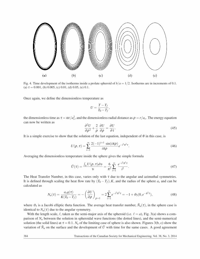
Fig. 4. Time development of the isotherms inside a prolate spheroid of b/a = 1/2. Isotherms are in increments of 0.1.(a) τ = 0.001, (b) 0.005, (c) 0.01, (d) 0.05, (e) 0.1.

Once again, we define the dimensionless temperature as

U =T −Tf

T0−Tf,

the dimensionless time as τ =αt/a2s , and the dimensionless radial distance as ρ = r/as. The energy equation

can now be written as∂ 2U∂ρ2 +

2ρ

∂U∂ρ

=∂U∂τ

. (45)

It is a simple exercise to show that the solution of the last equation, independent of θ in this case, is

U(ρ,τ) =∞

∑i=1

2(−1)i+1 sin(iπρ)

iπρe−i2π2τ . (46)

Averaging the dimensionless temperature inside the sphere gives the simple formula

U(τ) =

∫υ

U(ρ,τ)dυ

υ=

6π2

∞

∑i=1

e−i2π2τ

i2. (47)

The Heat Transfer Number, in this case, varies only with τ due to the angular and azimuthal symmetries.It is defined through scaling the heat flow rate by (T0−Tf ),K, and the radius of the sphere as and can becalculated as

Nu(τ) =asq(τ)

K(T0−Tf )=−

(∂U∂ρ

)ρ=1

= 2∞

∑i=1

e−i2π2τ =−1+ϑ3(0,e−π2τ), (48)

where ϑ3 is a Jacobi elliptic theta function. The average heat transfer number, Nu(τ), in the sphere case isidentical to Nu(τ) due to the angular symmetry.

With the length scale, `, taken as the semi-major axis of the spheroid (i.e. `= a), Fig. 3(a) shows a com-parison of Nu between the solution in spheroidal wave functions (the dotted lines), and the semi-numericalsolution (the solid lines) at τ = 0.1. Nu of the limiting case of sphere is also shown. Figures 3(b, c) show thevariation of Nu on the surface and the development of U with time for the same cases. A good agreement


Fig. 5. Time development of Nu on the surface of the spheroid of b/a = 1/2. (a) Prolate, (b) Oblate.

is observed. The solutions in terms of spheroidal wave functions are obtained using only six eigenfunctionswith six eigenvalues each. The numerical solution is obtained with tolerance between consecutive iterationsof 10−8.

Figure 4 shows the time development of the isotherms inside a prolate spheroid of b/a= 1/2. The initiallyhigh heat transfer rate on the surface which has little influence on the temperature deeper inside the spheroidsubsides with time. The time development of the heat transfer rate on the surface of a prolate spheroidof b/a = 1/2 is shown in Fig. 5(a) while that for an oblate spheroid of b/a = 1/2 is shown in Fig. 5(b).The maximum heat transfer rate, in the case of a prolate spheroid, occurs at η = 90 (i.e. at the flat partor minimum curvature), while it occurs at η = 0,180 (again at the flat portions) in the case of an oblatespheroid.

Considering the length scale to be the semi-major axis facilitates comparing spheroids having the samelength of the major axis and different axis ratios. Figure 6 shows the isotherms for oblate spheroids withvarying axis ratios. The isotherms are shot at τ = 0.01.

Figure 7 shows the distribution of Nu on the surface for spehroids with varying axis ratios at τ = 0.1.Figure 8 shows the development of Nu with time.

The temperature variations from the surface of a spheroid to its core may suggest that one needs to cal-culate the average temperature, U(τ) in Eq. (43), as a measure of the energy remaining inside the spheroid.Figure 9 shows the development of U(τ) for prolate and oblate spheroids with different axis ratios. Thefigure indicates that prolate spheroids lose energy faster than oblate spheroids with equal axis ratios. Oneshould not forget, however, that prolate spheroids are smaller in volume than oblate spheroids with equalmajor axes and equal axis ratios.

So far, we have compared spheroids based on the length scale, `, taken as the semi-major axis of thespheroid (i.e. ` = a). This practically means that all the spheroids have the same length of the major axis.Obviously, comparing two spheroids with equal major axes may not be “fair” as their two volumes areobviously different. It would be reasonable to compare spheroids having different axis ratios but the same


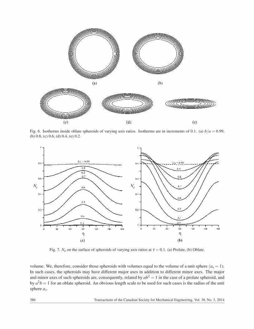
Fig. 6. Isotherms inside oblate spheroids of varying axis ratios. Isotherms are in increments of 0.1. (a) b/a = 0.99,(b) 0.8, (c) 0.6, (d) 0.4, (e) 0.2.

Fig. 7. Nu on the surface of spheroids of varying axis ratios at τ = 0.1. (a) Prolate, (b) Oblate.

volume. We, therefore, consider those spheroids with volumes equal to the volume of a unit sphere (as = 1).In such cases, the spheroids may have different major axes in addition to different minor axes. The majorand minor axes of such spheroids are, consequently, related by ab2 = 1 in the case of a prolate spheroid, andby a2b = 1 for an oblate spheroid. An obvious length scale to be used for such cases is the radius of the unitsphere as.


Fig. 8. Development of Nu for spheroids of varying axis ratios. (a) Prolate, (b) Oblate.

Fig. 9. Development of U for spheroids of varying axis ratios. (a) Prolate, (b) Oblate.

Figure 10 shows the development of U(τ) for prolate and oblate spheroids with equal volumes. Aninteresting feature of the figure is that for small axis ratios, an oblate spheroid transfers heat to the infinitemedium faster than a prolate spheroid with the same axis ratio and the same volume. For large axis ratios,there is little dependence of the heat transfer rate on the axis ratio. Furthermore, there is no significantdifference in the heat transfer rate for spheroids of either type. This is not unexpected and can be wellexplained by the fact that, for small axis ratios, the surface area of an oblate spheroid is much larger than thesurface area of a prolate spheroid which has the same volume. At large axis ratios, as shown in Fig. 11, thetwo surface areas are almost equal.


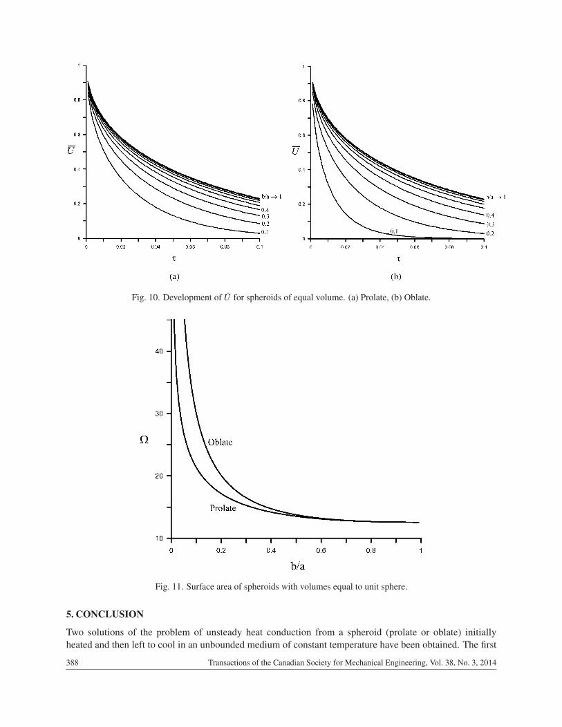
Fig. 10. Development of U for spheroids of equal volume. (a) Prolate, (b) Oblate.

Fig. 11. Surface area of spheroids with volumes equal to unit sphere.

5. CONCLUSION

Two solutions of the problem of unsteady heat conduction from a spheroid (prolate or oblate) initiallyheated and then left to cool in an unbounded medium of constant temperature have been obtained. The first


makes use of the spheroidal wave functions as basis and is given in Eq. (23) with the coefficients givenin Eq. (30). The second, which is numerical, is obtained by expanding the dimensionless temperature interms of Legendre functions (Eq. 32) and then solving the resulting set of differential equations (Eq. 33)in the radial direction using an implicit finite difference scheme. The two solutions have been verified bycomparing them to the limiting case of a sphere (Eq. 46). The effect of the axis ratio on the time developmentof temperature inside the spheroid and the heat flux across the surface has been studied.

ACKNOWLEDGEMENT

We would like to express our sincere appreciation to King Fahd University of Petroleum & Minerals(KFUPM) for supporting this research under Research Grant IN100035.

REFERENCES

1. Williams, M. M. R., “Thermophoretic forces acting on a spheroid”, Journal of Physics D: Applied Physics,Vol. 19, pp. 1631–1642, 1986.

2. Niven, C., “On the conduction of heat in ellipsoids of revolution”, Philosophical Transactions of the RoyalSociety London, Vol. 171, pp. 117–151, 1880.

3. Falloon, P.E., Abbott, P.C. and Wang, J.B., “Theory and Computation of the Spheroidal Wave Functions”, Jour-nal of Physics A: Mathematical and General, Vol. 36, No. 20, pp. 5477–5495, 2003.

4. Flammer, C., Spheroidal Wave Functions, Stanford University Press, Stanford, CA, 1957.5. Abramowitz, M. and Stegun, I. A. , Handbook of Mathematical Functions, 9th ed., Dover/New York, 1970.6. Stratton, J. A., Electromagnetic Theory, McGraw-Hill, New York, 1941.7. Meixner, J., Sch’afke, F.W. and Wolf, G., Mathieu Functions and Spheroidal Functions and Their Mathematical

Foundations, Lecture Notes in Mathematics, Vol. 837, Springer-Verlag, New York, NY, 1980.8. Caldwell, J., “Computation of eigenvalues of spheroidal harmonics using relaxation”, Journal of Physics A:

Mathematical and General, Vol. 21, No. 19, pp. 3685–3693, 1988.9. Hodge, D.B., “Eigenvalues and eigenfunctions of spheroidal wave equation”, Journal of Mathematical Physics,

Vol. 11, No. 8, pp. 2308, 1970.10. Baker, L., Mathematical Function Handbook, McGraw Hill, New York, 1992.11. Li, L.W., Kang, X.K. and Leong, M.S., Spheroidal Wave Functions in Electromagnetic Theory, Wiley, 2002.12. Zayed, A.I., “A generalization of the prolate spheroidal wave functions”, Proceedings of the American Mathe-

matical Society, Vol. 135, No.7, pp. 2193–2203, 2007.13. Ivers, D. J., “An angular spectral method of the solution of the heat equation in spheroidal geometries”, ANZIAM

J., Vol. 46(E), pp. C854–C870, 2005.14. Alassar, R.S., “Heat conduction from spheroids”, ASME Journal of Heat Transfer, Vol. 121, pp. 497–499, 1999.15. Arfken, G., Mathematical Methods for Physicists, 3rd ed. Orlando, FL: Academic Press, 1985.16. Moon, P. and Spencer, D.E., Field Theory Handbook, Springer-Verlag, Berlin/Heidelberg/New York, 1971.17. Morse, P.M. and Feshbach, H, Methods of Theoretical Physics, Part I. New York: McGraw-Hill, 1953.


transient heat conduction from · pdf filetransient heat conduction from spheroids rajai...

Documents