1

TRANSIENT RECOVERY VOLTAGE (TRV) FOR HIGH-VOLTAGECIRCUIT BREAKERS

R.W.Alexander, PPL, Senior Member IEEE

D.Dufournet, Alstom T&D, Senior Member IEEE

1 GeneralThe recovery voltage is the voltage which appears across the terminals of a pole of a circuit breaker.This voltage may be considered in two successive time intervals: one during which a transient voltageexists, followed by a second one during which a power frequency voltage alone exists.

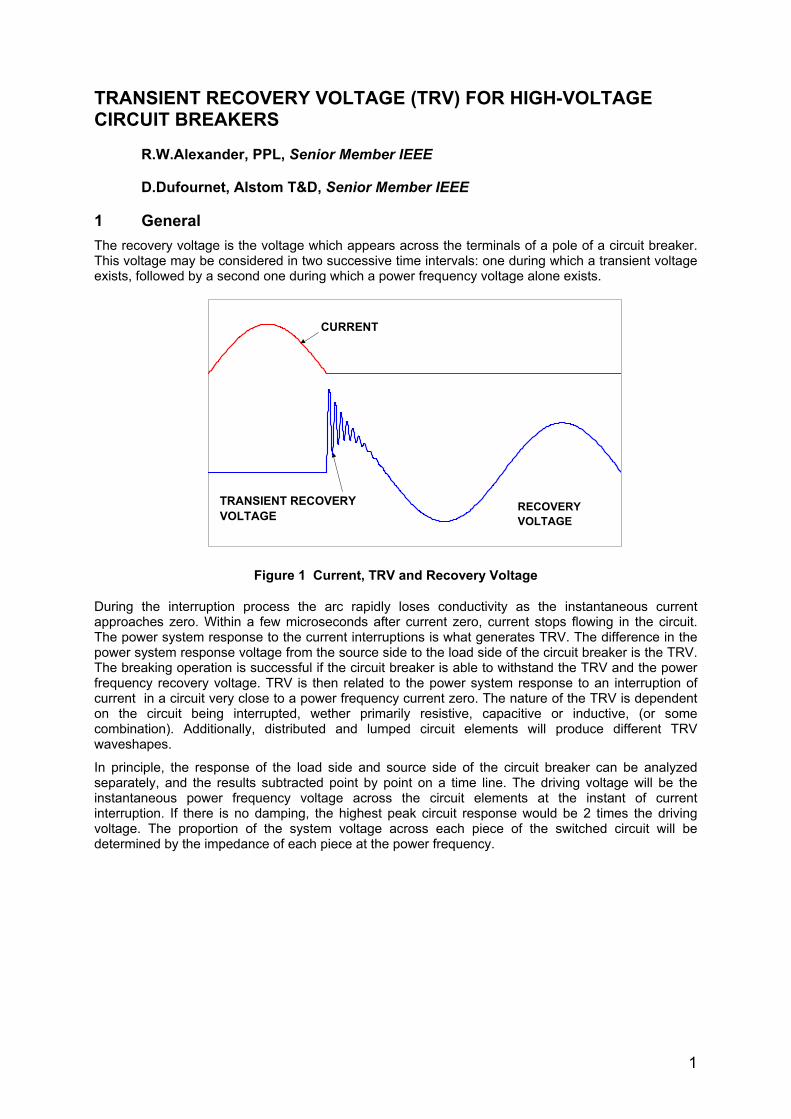
Figure 1 Current, TRV and Recovery Voltage

During the interruption process the arc rapidly loses conductivity as the instantaneous currentapproaches zero. Within a few microseconds after current zero, current stops flowing in the circuit.The power system response to the current interruptions is what generates TRV. The difference in thepower system response voltage from the source side to the load side of the circuit breaker is the TRV.The breaking operation is successful if the circuit breaker is able to withstand the TRV and the powerfrequency recovery voltage. TRV is then related to the power system response to an interruption ofcurrent in a circuit very close to a power frequency current zero. The nature of the TRV is dependenton the circuit being interrupted, wether primarily resistive, capacitive or inductive, (or somecombination). Additionally, distributed and lumped circuit elements will produce different TRVwaveshapes.

In principle, the response of the load side and source side of the circuit breaker can be analyzedseparately, and the results subtracted point by point on a time line. The driving voltage will be theinstantaneous power frequency voltage across the circuit elements at the instant of currentinterruption. If there is no damping, the highest peak circuit response would be 2 times the drivingvoltage. The proportion of the system voltage across each piece of the switched circuit will bedetermined by the impedance of each piece at the power frequency.

CURRENT

TRANSIENT RECOVERYVOLTAGE

RECOVERY VOLTAGE

2

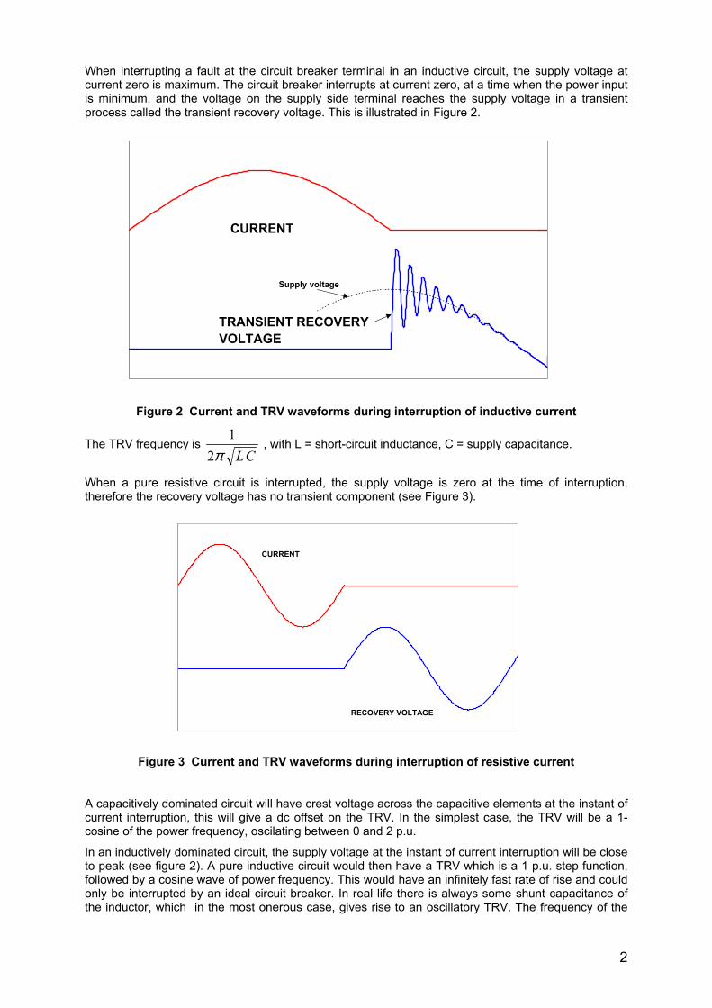
When interrupting a fault at the circuit breaker terminal in an inductive circuit, the supply voltage atcurrent zero is maximum. The circuit breaker interrupts at current zero, at a time when the power inputis minimum, and the voltage on the supply side terminal reaches the supply voltage in a transientprocess called the transient recovery voltage. This is illustrated in Figure 2.

Figure 2 Current and TRV waveforms during interruption of inductive current

The TRV frequency is CLπ2

1 , with L = short-circuit inductance, C = supply capacitance.

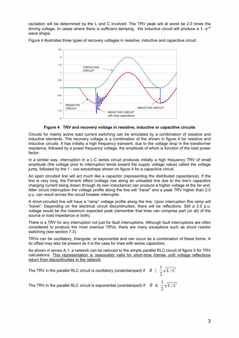
When a pure resistive circuit is interrupted, the supply voltage is zero at the time of interruption,therefore the recovery voltage has no transient component (see Figure 3).

Figure 3 Current and TRV waveforms during interruption of resistive current

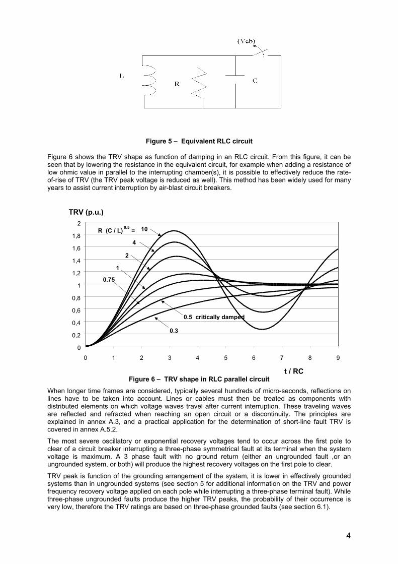
A capacitively dominated circuit will have crest voltage across the capacitive elements at the instant ofcurrent interruption, this will give a dc offset on the TRV. In the simplest case, the TRV will be a 1-cosine of the power frequency, oscilating between 0 and 2 p.u.

In an inductively dominated circuit, the supply voltage at the instant of current interruption will be closeto peak (see figure 2). A pure inductive circuit would then have a TRV which is a 1 p.u. step function,followed by a cosine wave of power frequency. This would have an infinitely fast rate of rise and couldonly be interrupted by an ideal circuit breaker. In real life there is always some shunt capacitance ofthe inductor, which in the most onerous case, gives rise to an oscillatory TRV. The frequency of the

CURRENT

RECOVERY VOLTAGE

CURRENT

TRANSIENT RECOVERYVOLTAGE

Supply voltage

3

oscilation will be determined by the L and C involved. The TRV peak will at worst be 2.0 times thedriving voltage. In cases where there is sufficient damping, the inductive circuit will produce a 1- e-αt

wave shape.

Figure 4 illustrates three types of recovery voltages in resistive, inductive and capacitive circuit.

Figure 4 TRV and recovery voltage in resistive, inductive or capacitive circuitsCircuits for mainly active load current switching can be simulated by a combination of resistive andinductive elements. The recovery voltage is a combination of the shown in figure 4 for resistive andinductive circuits. It has initially a high frequency transient, due to the voltage drop in the transformerreactance, followed by a power frequency voltage, the amplitude of which is function of the load powerfactor.

In a similar way, interruption in a L-C series circuit produces initially a high frequency TRV of smallamplitude (the voltage prior to interruption tends toward the supply voltage value) called the voltagejump, followed by the 1 - cos waveshape shown on figure 4 for a capacitive circuit.

An open circuited line will act much like a capacitor (representing the distributed capacitance). If theline is very long, the Ferranti effect (voltage rise along an unloaded line due to the line’s capacitivecharging current being drawn through its own inductance) can produce a higher voltage at the far end.After circuit interruption the voltage profile along the line will “travel” and a peak TRV higher than 2.0p.u. can result across the circuit breaker interrupter.

A short-circuited line will have a “ramp” voltage profile along the line. Upon interruption this ramp will“travel”. Depending on the electrical circuit discontinuities, there will be reflections. Still a 2.0 p.u.voltage would be the maximum expected peak (remember that lines can comprise part (or all) of thesource or load impedance or both).

There is a TRV for any interruption not just for fault interruptions. Although fault interruptions are oftenconsidered to produce the most onerous TRVs, there are many exceptions such as shunt reactorswitching (see section 7.3).

TRVs can be oscillatory, triangular, or exponential and can occur as a combination of these forms. Adc offset may also be present as it is the case for lines with series capacitors.

As shown in annex A.1, a network can be reduced to the simple parallel RLC circuit of figure 5 for TRVcalculations. This representation is reasonably valid for short-time frames until voltage reflectionsreturn from discontinuities in the network.

The TRV in the parallel RLC circuit is oscillatory (underdamped) if CLR /21

⟩

The TRV in the parallel RLC circuit is exponential (overdamped) if CLR /21≤

-2

-1,5

-1

-0,5

0

0,5

1

1,5

2

2,5

RESISTIVE CIRCUIT

INDUCTIVE CIRCUITwith stray capacitance

CAPACITIVE CIRCUIT

INDUCTIVE CIRCUIT

4

Figure 5 – Equivalent RLC circuit

Figure 6 shows the TRV shape as function of damping in an RLC circuit. From this figure, it can beseen that by lowering the resistance in the equivalent circuit, for example when adding a resistance oflow ohmic value in parallel to the interrupting chamber(s), it is possible to effectively reduce the rate-of-rise of TRV (the TRV peak voltage is reduced as well). This method has been widely used for manyyears to assist current interruption by air-blast circuit breakers.

Figure 6 – TRV shape in RLC parallel circuitWhen longer time frames are considered, typically several hundreds of micro-seconds, reflections onlines have to be taken into account. Lines or cables must then be treated as components withdistributed elements on which voltage waves travel after current interruption. These traveling wavesare reflected and refracted when reaching an open circuit or a discontinuity. The principles areexplained in annex A.3, and a practical application for the determination of short-line fault TRV iscovered in annex A.5.2.

The most severe oscillatory or exponential recovery voltages tend to occur across the first pole toclear of a circuit breaker interrupting a three-phase symmetrical fault at its terminal when the systemvoltage is maximum. A 3 phase fault with no ground return (either an ungrounded fault ,or anungrounded system, or both) will produce the highest recovery voltages on the first pole to clear.

TRV peak is function of the grounding arrangement of the system, it is lower in effectively groundedsystems than in ungrounded systems (see section 5 for additional information on the TRV and powerfrequency recovery voltage applied on each pole while interrupting a three-phase terminal fault). Whilethree-phase ungrounded faults produce the higher TRV peaks, the probability of their occurrence isvery low, therefore the TRV ratings are based on three-phase grounded faults (see section 6.1).

0

0,2

0,4

0,6

0,8

1

1,2

1,4

1,6

1,8

2

0 1 2 3 4 5 6 7 8 9

TRV (p.u.)

R (C / L) 0.5 = 10

4

2

1

0.75

0.5 critically damped

0.3

t / RC

5

By definition, all TRV values defined in the standards are inherent, i.e. the values that would beobtained during interruption by an ideal circuit breaker without arc voltage (its resistance changes fromzero to an infinite value at current zero).

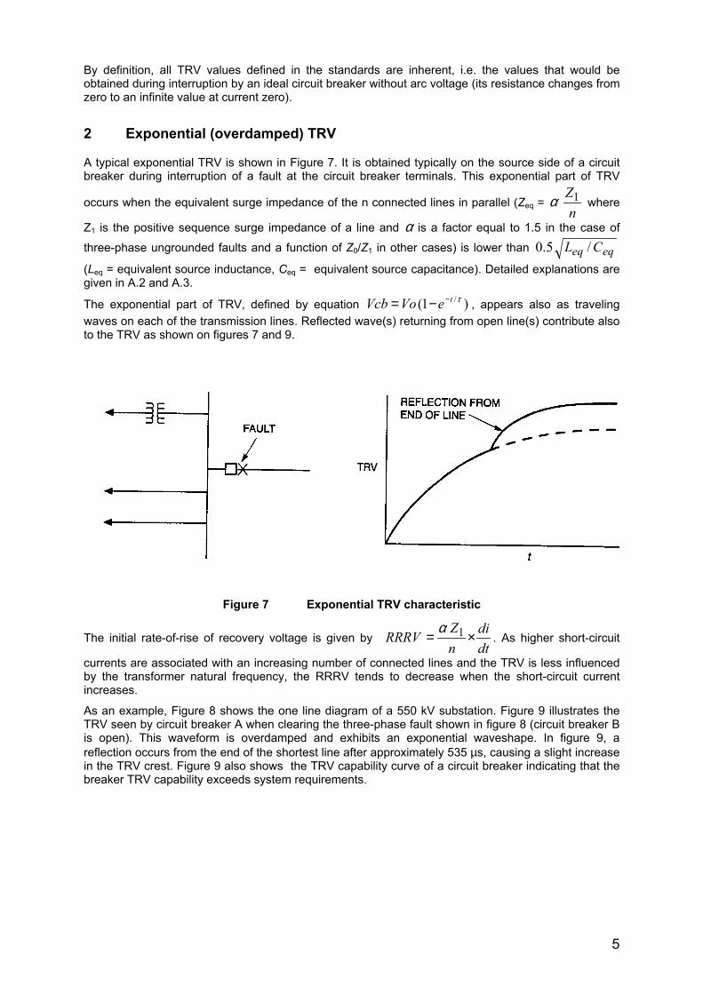
2 Exponential (overdamped) TRV

A typical exponential TRV is shown in Figure 7. It is obtained typically on the source side of a circuitbreaker during interruption of a fault at the circuit breaker terminals. This exponential part of TRV

occurs when the equivalent surge impedance of the n connected lines in parallel (Zeq = n

Z1α where

Z1 is the positive sequence surge impedance of a line and α is a factor equal to 1.5 in the case ofthree-phase ungrounded faults and a function of Z0/Z1 in other cases) is lower than eqeq CL /5.0(Leq = equivalent source inductance, Ceq = equivalent source capacitance). Detailed explanations aregiven in A.2 and A.3.

The exponential part of TRV, defined by equation )1( /τteVoVcb −−= , appears also as travelingwaves on each of the transmission lines. Reflected wave(s) returning from open line(s) contribute alsoto the TRV as shown on figures 7 and 9.

Figure 7 Exponential TRV characteristic

The initial rate-of-rise of recovery voltage is given by dtdi

nZ

RRRV ×= 1α. As higher short-circuit

currents are associated with an increasing number of connected lines and the TRV is less influencedby the transformer natural frequency, the RRRV tends to decrease when the short-circuit currentincreases.

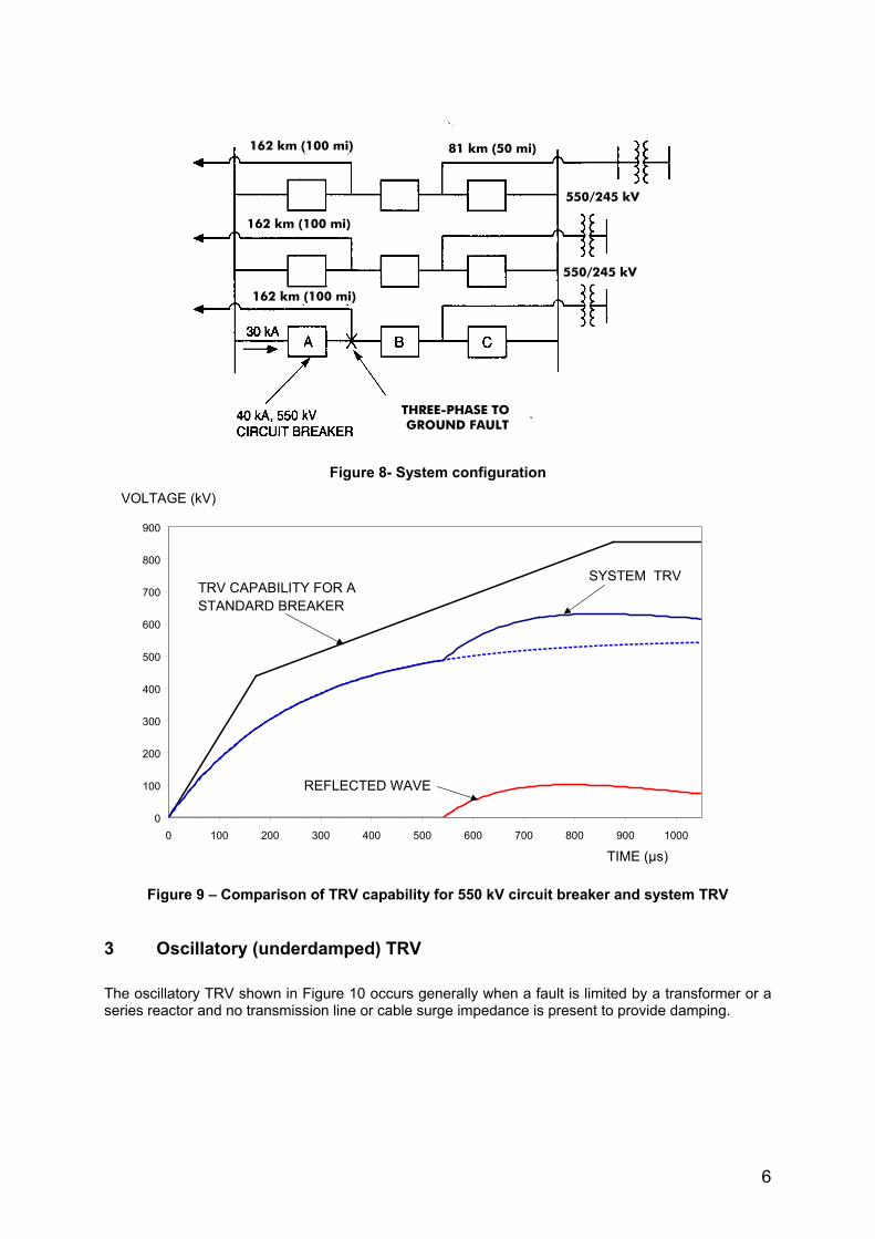
As an example, Figure 8 shows the one line diagram of a 550 kV substation. Figure 9 illustrates theTRV seen by circuit breaker A when clearing the three-phase fault shown in figure 8 (circuit breaker Bis open). This waveform is overdamped and exhibits an exponential waveshape. In figure 9, areflection occurs from the end of the shortest line after approximately 535 µs, causing a slight increasein the TRV crest. Figure 9 also shows the TRV capability curve of a circuit breaker indicating that thebreaker TRV capability exceeds system requirements.

6

Figure 8- System configuration

Figure 9 – Comparison of TRV capability for 550 kV circuit breaker and system TRV

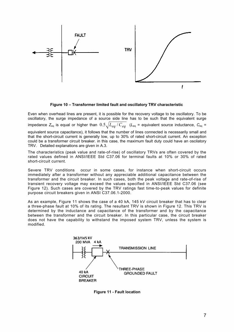
3 Oscillatory (underdamped) TRV

The oscillatory TRV shown in Figure 10 occurs generally when a fault is limited by a transformer or aseries reactor and no transmission line or cable surge impedance is present to provide damping.

162 km (100 mi) 81 km (50 mi)

THREE-PHASE TO GROUND FAULT

162 km (100 mi)

162 km (100 mi)

550/245 kV

550/245 kV

0

100

200

300

400

500

600

700

800

900

0 100 200 300 400 500 600 700 800 900 1000

TIME (µs)

VOLTAGE (kV)

SYSTEM TRVTRV CAPABILITY FOR A STANDARD BREAKER

REFLECTED WAVE

7

Figure 10 – Transformer limited fault and oscillatory TRV characteristic

Even when overhead lines are present, it is possible for the recovery voltage to be oscillatory. To beoscillatory, the surge impedance of a source side line has to be such that the equivalent surgeimpedance Zeq is equal or higher than eqeq CL /5.0 (Leq = equivalent source inductance, Ceq =

equivalent source capacitance), it follows that the number of lines connected is necessarily small andthat the short-circuit current is generally low, up to 30% of rated short-circuit current. An exceptioncould be a transformer circuit breaker. in this case, the maximum fault duty could have an oscilatoryTRV. Detailed explanations are given in A.3. The characteristics (peak value and rate-of-rise) of oscillatory TRVs are often covered by therated values defined in ANSI/IEEE Std C37.06 for terminal faults at 10% or 30% of ratedshort-circuit current.

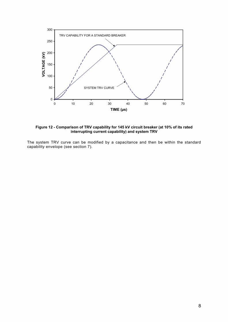
Severe TRV conditions occur in some cases, for instance when short-circuit occursimmediately after a transformer without any appreciable additional capacitance between thetransformer and the circuit breaker. In such cases, both the peak voltage and rate-of-rise oftransient recovery voltage may exceed the values specified in ANSI/IEEE Std C37.06 (seeFigure 12). Such cases are covered by the TRV ratings fast time-to-peak values for definitepurpose circuit breakers given in ANSI C37.06.1-2000.

As an example, Figure 11 shows the case of a 40 kA, 145 kV circuit breaker that has to cleara three-phase fault at 10% of its rating. The resultant TRV is shown in Figure 12. This TRV isdetermined by the inductance and capacitance of the transformer and by the capacitancebetween the transformer and the circuit breaker. In this particular case, the circuit breakerdoes not have the capability to withstand the imposed system TRV, unless the system ismodified.

Figure 11 - Fault location

8

Figure 12 - Comparison of TRV capability for 145 kV circuit breaker (at 10% of its ratedinterrupting current capability) and system TRV

The system TRV curve can be modified by a capacitance and then be within the standardcapability envelope (see section 7).

0

50

100

150

200

250

300

0 10 20 30 40 50 60 70

TIME (µs)

VOLT

AG

E (k

V)

SYSTEM TRV CURVE

TRV CAPABILITY FOR A STANDARD BREAKER

9

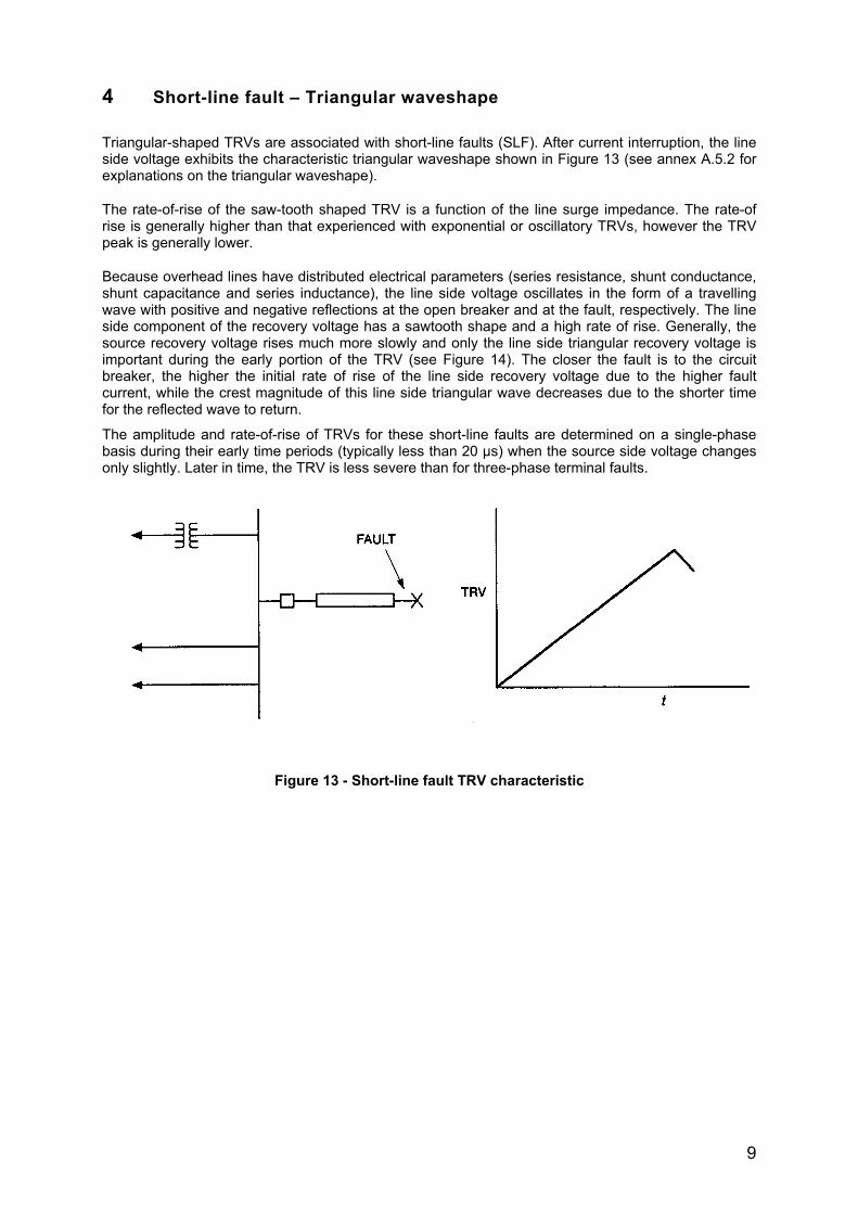
4 Short-line fault – Triangular waveshape

Triangular-shaped TRVs are associated with short-line faults (SLF). After current interruption, the lineside voltage exhibits the characteristic triangular waveshape shown in Figure 13 (see annex A.5.2 forexplanations on the triangular waveshape).

The rate-of-rise of the saw-tooth shaped TRV is a function of the line surge impedance. The rate-ofrise is generally higher than that experienced with exponential or oscillatory TRVs, however the TRVpeak is generally lower.

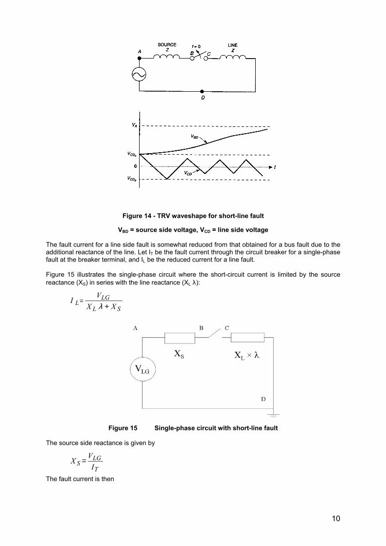
Because overhead lines have distributed electrical parameters (series resistance, shunt conductance,shunt capacitance and series inductance), the line side voltage oscillates in the form of a travellingwave with positive and negative reflections at the open breaker and at the fault, respectively. The lineside component of the recovery voltage has a sawtooth shape and a high rate of rise. Generally, thesource recovery voltage rises much more slowly and only the line side triangular recovery voltage isimportant during the early portion of the TRV (see Figure 14). The closer the fault is to the circuitbreaker, the higher the initial rate of rise of the line side recovery voltage due to the higher faultcurrent, while the crest magnitude of this line side triangular wave decreases due to the shorter timefor the reflected wave to return.

The amplitude and rate-of-rise of TRVs for these short-line faults are determined on a single-phasebasis during their early time periods (typically less than 20 µs) when the source side voltage changesonly slightly. Later in time, the TRV is less severe than for three-phase terminal faults.

Figure 13 - Short-line fault TRV characteristic

10

Figure 14 - TRV waveshape for short-line fault

VBD = source side voltage, VCD = line side voltage

The fault current for a line side fault is somewhat reduced from that obtained for a bus fault due to theadditional reactance of the line. Let IT be the fault current through the circuit breaker for a single-phasefault at the breaker terminal, and IL be the reduced current for a line fault.

Figure 15 illustrates the single-phase circuit where the short-circuit current is limited by the sourcereactance (XS) in series with the line reactance (XL λ):

SL

LGL XX

VI

+=

λ

Figure 15 Single-phase circuit with short-line fault

The source side reactance is given by

T

LGS I

VX =

The fault current is then

11

TLGL

LGL IVX

VI

/+=

λwhere

XL is (2 L1w + L0w ) ω / 3XL is the reactance of the line to the fault point per unit lengthL1w is the positive sequence power frequency line inductance per unit lengthL0w is the zero sequence power frequency line inductance per unit lengthVLG is the system line-ground voltageλ is the distance from the opening circuit-breaker to the fault

In general, it is not necessary to calculate the SLF TRV as long as the terminal fault TRVs are withinrating and transmission line parameters are within the values specified in ANSI/IEEE Std C37.04. Thetransmission line parameters are given in terms of the effective surge impedance, Zeff, of the faultedline and the peak factor, d, defined as:

vXZ

dL

effω2=

where:

Zeff = (2Z1 + Z0)/3v is the velocity of lightZeff is the effective surge impedance of the lineZ1 is the positive sequence surge impedanceZ0 is the zero sequence surge impedanceω is 2 π × system power frequency (377 rad/s for a 60 Hz system)

Annex A.5 gives equations for the calculation of the peak factor d as function of system parameters.The rate of rise of recovery voltage on the line side (RL) is given by the following formula, as functionof the fault current (IL) and the line surge impedance (Z):

ZIR LL ω2=

The first peak of TRV seen across the circuit-breaker terminals is the sum of a line-side contribution(eL) and a source-side contribution (eS):

SL eee +=

kVEMdeL max3/2)1( −=

)(2 dLS tTMe −=

where td is the time delay of TRV on the source side

TL is the time to peak L

LL R

eT =

M is the ratio of the fault current to the rated short circuit currentEmax is the rated maximum voltage (kV)

This rate-of-rise during SLF is significantly higher than the values that are met during terminal faultinterruption:

10.8 kV/µs for SLF with IL = 45 kA, Z = 450 Ω and a 60 Hz system

8.64 kV/µs for SLF with IL = 36 kA, Z = 450 Ω and a 60 Hz system

3 kV/µs for Terminal fault at 60 % of rated breaking current

2 kV/µs for Terminal fault at 100% of rated breaking current

12

The high rate-of-rise of SLF associated with high fault currents (of 45 kA or higher) can be difficult towithstand by circuit breakers. In order to assist the circuit breaker during the interruption, a phase toground capacitor, or a capacitor(s) in parallel to the interrupting chamber(s), can be used to reduce therate-of-rise of recovery voltage (RRRV).

When a phase-to-ground capacitor is used, the reduction of line side RRRV is given by

CaddCCIZ

RRRVL

LLL 5.2

2+

=ω

where

2ZXC L

Lωλ= is the total line capacitance

Cadd is the additional phase-to-ground capacitance

5 First pole-to-clear factor

The first–pole–to-clear factor (kpp) is a function of the grounding arrangements of the system.It is the ratio of the power frequency voltage across the interrupting pole before currentinterruption in the other poles, to the power frequency voltage occurring across the pole orpoles after interruption in all three poles.

For systems with ungrounded neutral, kpp is or tends towards 1.5. Such systems can be metwith rated voltages less than 245 kV, however at transmission voltages, i.e. greater than72.5kV, it is increasingly rare and effective grounding is the norm.

For effectively grounded neutral systems, the realistic and practical value is dependent uponthe sequence impedances of the actual earth paths from the location of the fault to thevarious system neutral points (ratio X0/X1). For these systems the ratio X0/X1 is taken to be ≤ 3.0. Three-phase to ground faults are the basis for rating because it is recognised thatthree-phase ungrounded faults have a very low probability of occurrence. For voltages, lessthan 100 kV, the case of three-phase ungrounded faults is uncommon, however the situationis automatically covered in the Standards since a first pole to clear factor of 1.5 is specified tocover three-phase faults in non effectively grounded systems.

For special applications in transmission systems with effectively grounded neutral where theprobability of three-phase ungrounded faults cannot be disregarded, a first-pole-to-clear factorof 1.5 may be required.

For rating purposes, two values of the first-pole to clear factor are defined for the three-phaseshort-circuit condition. The choice between these two values is dependent on the systemgrounding arrangement:

a) systems with ungrounded neutral: a standardised value for kpp of 1.5 is used;b) effectively grounded systems: for standardisation purposes the value for kpp used is 1.3.

A third condition does exist, this is where the fault is single-phase in an effectively groundedsystem and the last-pole-to-clear is considered. For this kpp is 1.0.

Generally it will not be necessary to consider alternative transient recovery voltages as thestandard values specified cover the majority of practical cases.

- Formula for the first-pole-to-clear factor

01

02

3XX

Xk pp +

= ,

where X0 is the zero sequence, and X1 the positive sequence reactance of the system.

13

If X0 >> X1, as in ungrounded systems then: kpp = 1.5If X0 = 3.0 X1, as in effectively grounded neutral systems then: kpp = 1.3

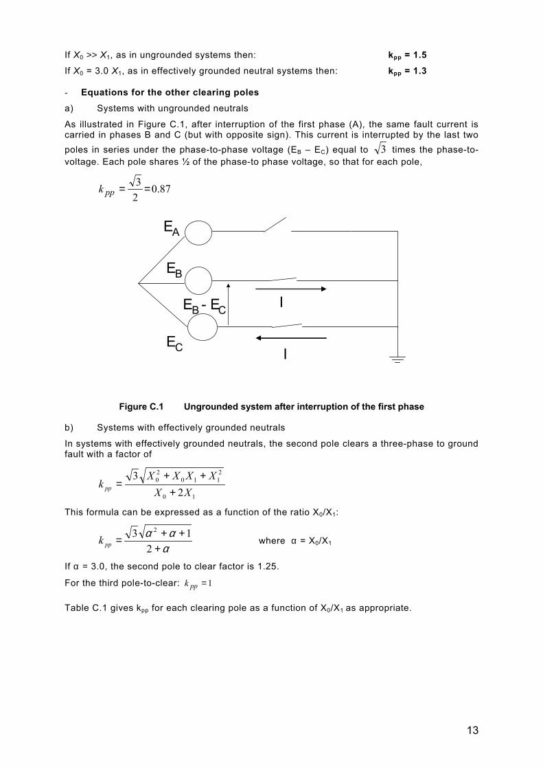
- Equations for the other clearing polesa) Systems with ungrounded neutrals

As illustrated in Figure C.1, after interruption of the first phase (A), the same fault current iscarried in phases B and C (but with opposite sign). This current is interrupted by the last twopoles in series under the phase-to-phase voltage (EB – EC) equal to 3 times the phase-to-voltage. Each pole shares ½ of the phase-to phase voltage, so that for each pole,

87.023 ==ppk

Figure C.1 Ungrounded system after interruption of the first phase

b) Systems with effectively grounded neutrals

In systems with effectively grounded neutrals, the second pole clears a three-phase to groundfault with a factor of

10

2110

20

23

XXXXXX

k pp +++

=

This formula can be expressed as a function of the ratio X0/X1:

ααα

+++=

213 2

ppk where α = X0/X1

If α = 3.0, the second pole to clear factor is 1.25.

For the third pole-to-clear: 1=ppk

Table C.1 gives kpp for each clearing pole as a function of X0/X1 as appropriate.

EA

EB

EC

I

I

EB - EC

14

Table C.1 - Pole-to-clear factors (kpp) for each pole when clearing three-phase to ground faults

neutral X0/X1 Pole-to-clear factor kpp

Ratio First Second Third

ungrounded Infinite 1.5 0.87 0.87

Effectivelygrounded

3.0 1.3 1.25 1.0

See note 1.00 1..0 1.00 1.0

Note: values of the pole-to-clear factor are given for Xo/X1 = 1.0 to indicate the trend in the specialcase of networks with a ratio Xo/X1 of less than 3.0.

It is important to note that as the amplitude factor is the same for each pole, the multiplying factors oftable C.1 are applicable to the power frequency voltages and to the TRV on each pole.

In the special case of three-phase ungrounded faults, the pole-to-clear factors are as defined in a) forthree-phase faults in ungrounded systems.

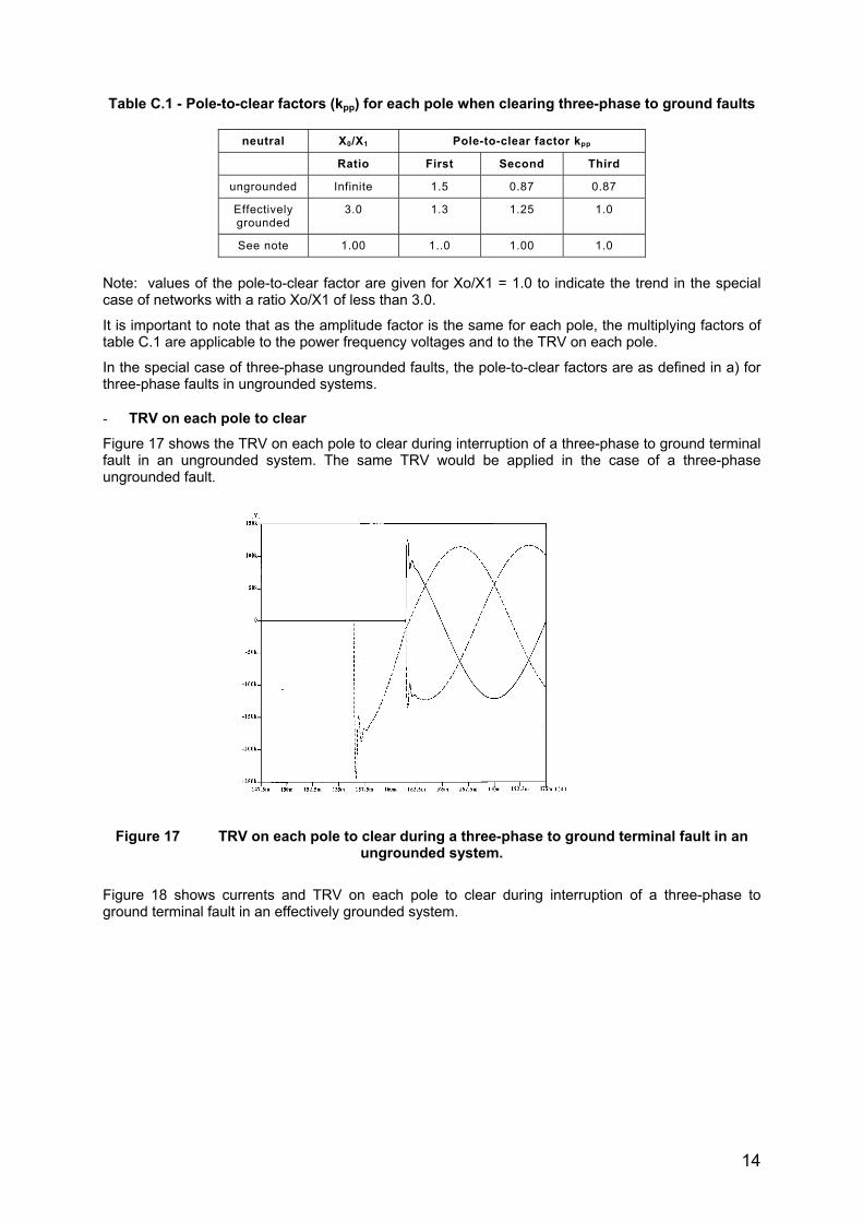
- TRV on each pole to clearFigure 17 shows the TRV on each pole to clear during interruption of a three-phase to ground terminalfault in an ungrounded system. The same TRV would be applied in the case of a three-phaseungrounded fault.

Figure 17 TRV on each pole to clear during a three-phase to ground terminal fault in anungrounded system.

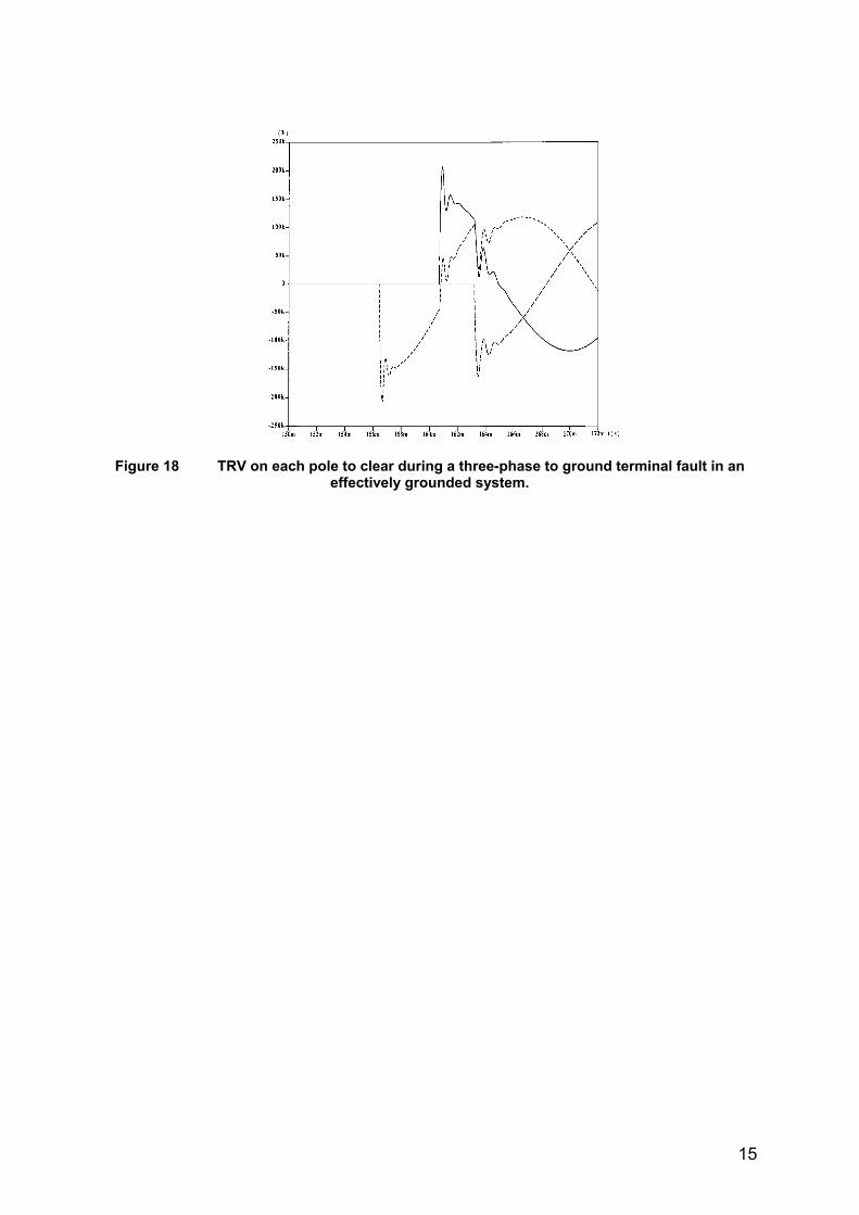
Figure 18 shows currents and TRV on each pole to clear during interruption of a three-phase toground terminal fault in an effectively grounded system.

15

Figure 18 TRV on each pole to clear during a three-phase to ground terminal fault in aneffectively grounded system.

16

6 Rating and testing

6.1 Terminal faultThe TRV ratings for circuit breakers are applicable for interrupting three-phase to ground faults at therated symmetrical short circuit current and at the maximum rated voltage of the circuit breaker. Forvalues of fault current other than rated and for line faults, related TRV capabilities are given. Ratedand related TRV capabilities are described in ANSI/IEEE Std C37.04 and given in detail in ANSIC37.06.

While three-phase ungrounded faults produce the highest TRV peaks, the probability of theiroccurrence is very low. Therefore, as described in ANSI/IEEE Std C37.04, the TRV ratings are basedon three-phase grounded faults with the TRV peaks established based on the groundingarrangements prevalent at the respective system voltages.

For circuit breakers applied on systems 72.5 kV and below, the TRV ratings assume that the systemscan be operated ungrounded. The first pole-to clear factor kpp is 1.5.

For circuit breakers applied on systems 245 kV and above, the TRV ratings assume that the systemsare all operated effectively grounded: the first pole-to-clear factor kpp is 1.3. For systems 100 through170 kV the systems can be operated either ungrounded or effectively grounded so two TRV ratingsare available for these systems (kpp = 1.3 or 1.5). In addition, for special applications in transmissionsystems where the probability of three-phase ungrounded faults cannot be disregarded, a first pole-to-clear factor of 1.5 may be required.

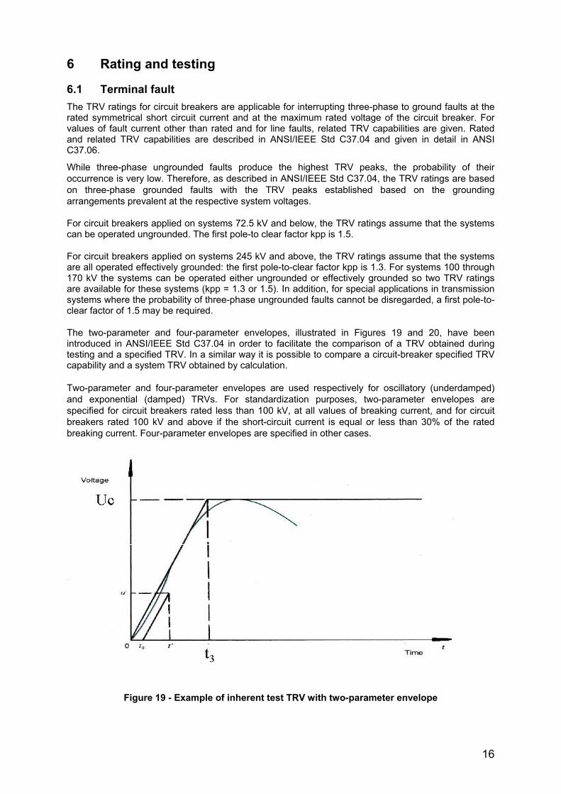
The two-parameter and four-parameter envelopes, illustrated in Figures 19 and 20, have beenintroduced in ANSI/IEEE Std C37.04 in order to facilitate the comparison of a TRV obtained duringtesting and a specified TRV. In a similar way it is possible to compare a circuit-breaker specified TRVcapability and a system TRV obtained by calculation.

Two-parameter and four-parameter envelopes are used respectively for oscillatory (underdamped)and exponential (damped) TRVs. For standardization purposes, two-parameter envelopes arespecified for circuit breakers rated less than 100 kV, at all values of breaking current, and for circuitbreakers rated 100 kV and above if the short-circuit current is equal or less than 30% of the ratedbreaking current. Four-parameter envelopes are specified in other cases.

Figure 19 - Example of inherent test TRV with two-parameter envelope

17

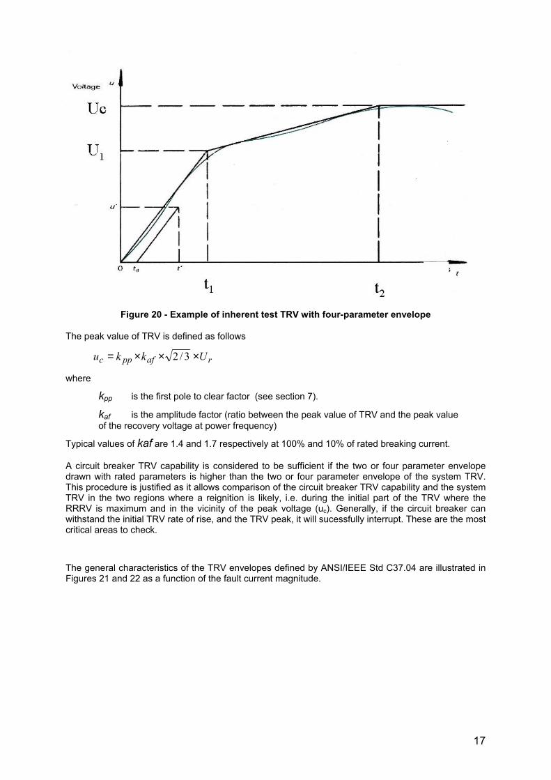
Figure 20 - Example of inherent test TRV with four-parameter envelope

The peak value of TRV is defined as follows

rafppc Ukku ×××= 3/2

where

kpp is the first pole to clear factor (see section 7).

kaf is the amplitude factor (ratio between the peak value of TRV and the peak value of the recovery voltage at power frequency)

Typical values of kaf are 1.4 and 1.7 respectively at 100% and 10% of rated breaking current.

A circuit breaker TRV capability is considered to be sufficient if the two or four parameter envelopedrawn with rated parameters is higher than the two or four parameter envelope of the system TRV.This procedure is justified as it allows comparison of the circuit breaker TRV capability and the systemTRV in the two regions where a reignition is likely, i.e. during the initial part of the TRV where theRRRV is maximum and in the vicinity of the peak voltage (uc). Generally, if the circuit breaker canwithstand the initial TRV rate of rise, and the TRV peak, it will sucessfully interrupt. These are the mostcritical areas to check.

The general characteristics of the TRV envelopes defined by ANSI/IEEE Std C37.04 are illustrated inFigures 21 and 22 as a function of the fault current magnitude.

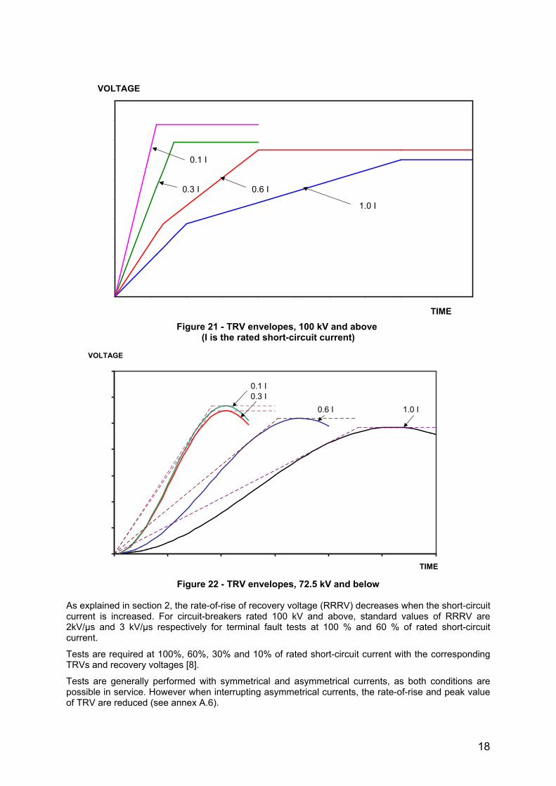
18

Figure 21 - TRV envelopes, 100 kV and above (I is the rated short-circuit current)

Figure 22 - TRV envelopes, 72.5 kV and below

As explained in section 2, the rate-of-rise of recovery voltage (RRRV) decreases when the short-circuitcurrent is increased. For circuit-breakers rated 100 kV and above, standard values of RRRV are2kV/µs and 3 kV/µs respectively for terminal fault tests at 100 % and 60 % of rated short-circuitcurrent.

Tests are required at 100%, 60%, 30% and 10% of rated short-circuit current with the correspondingTRVs and recovery voltages [8].

Tests are generally performed with symmetrical and asymmetrical currents, as both conditions arepossible in service. However when interrupting asymmetrical currents, the rate-of-rise and peak valueof TRV are reduced (see annex A.6).

TIME

VOLTAGE

1.0 I0.6 I0.3 I0.1 I

1.0 I

0.6 I0.3 I

0.1 I

TIME

VOLTAGE

19

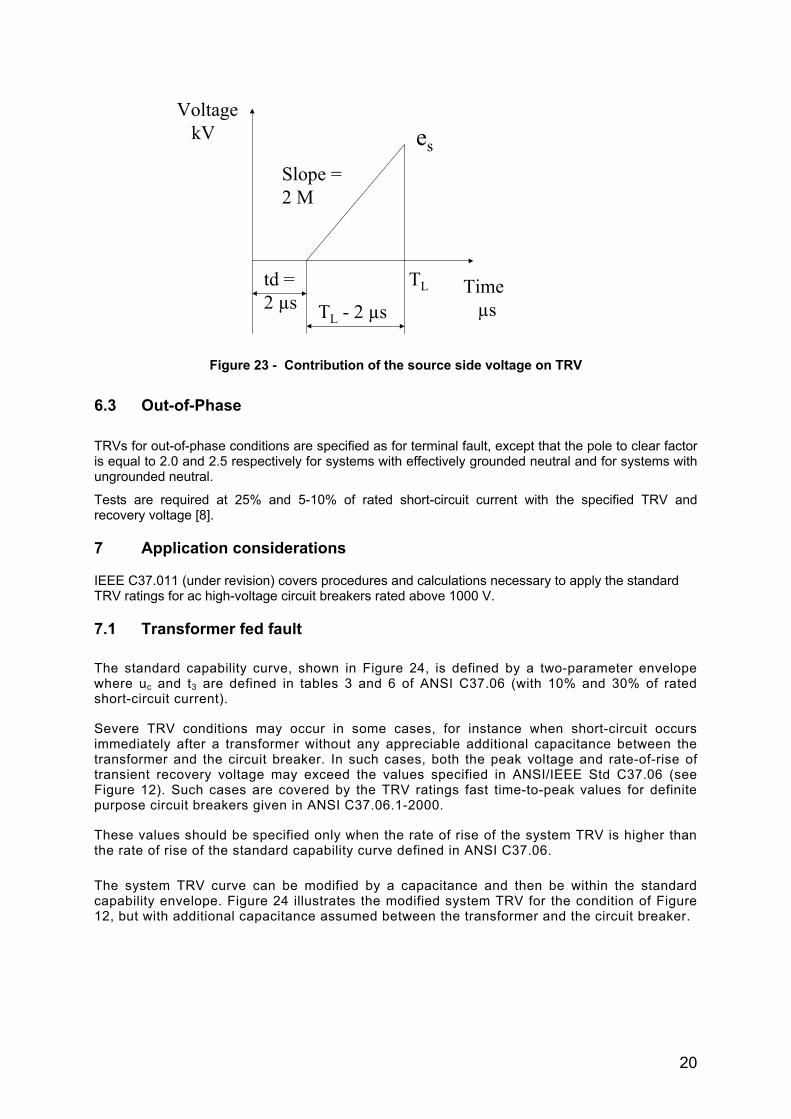
In a network, the initial part of the TRV may have an initial oscillation of small amplitude,called ITRV, due to reflections from the first major discontinuity along the busbar. The ITRV ismainly determined by the busbar and line bay configuration of the substation. The ITRV is aphysical phenomenon that is very similar to the short-line fault (see 6.2). Compared with theshort-line fault, the first voltage peak is rather low, but the time to the first peak is extremelyshort, within the first microseconds after current zero. If a circuit breaker has a short-line faultrating, the ITRV requirements are considered to be covered. Since the ITRV is proportional tothe busbar surge impedance and to the current, the ITRV requirements can be neglected forall circuit-breakers with a rated short-circuit breaking current of less than 25 kA and for circuit-breakers with a rated voltage below 100 kV. In addition the ITRV requirements can beneglected for circuit-breakers installed in metal enclosed gas insulated switchgear (GIS)because of the low surge impedance

6.2 Short line fault

The rated values for the line surge impedance Z and the peak factor d as defined in ANSI/IEEE StdC37.04 are as follows:

Z = 450 Ωd = 1.6

The line side contribution to the initial part of TRV is defined as a triangular wave in ANSI/IEEE StdC37.09 as follows:

kVUrMdeL 3/2)1( −=

µskVZIMRL /10.2 6−= ωTL = eL / RL µs

where

Le is the peak value of TRV on the line side (kV)RL is the rate-of-rise (kV/µs)TL is the time to peak (µs)M is the ratio of the fault current to the rated short circuit currentUr is the rated maximum voltage (kV)I is the rated short circuit current (kA)

As can be seen in Figure 14, the TRV across the interrupter is in reality the difference between thetransient recovery voltages on the supply and on the line side. As illustrated on Figure 23, the variationof the source side voltage increases the first peak value of TRV by es.

etotal = es + e

As a first approximation, the contribution from the source side voltage can be estimated by consideringthat the variation of the source side voltage is zero until time td = 2 µs (standard value of time delay),and then changes with a slope of 2 kV/µs (standard value of RRRV for terminal fault) up to time TL.

In this approximation, it is considered that the RRRV is the same as for three-phase terminal faults. Inreality it is reduced by the factor M as RRRV is proportional to the fault current (on the source sideRRRV = 2 × M).

es = (TL-2µs) x 2M

Tests are required at 90% and 75% of rated short-circuit current with the corresponding TRVs andrecovery voltages [8].

20

Figure 23 - Contribution of the source side voltage on TRV

6.3 Out-of-Phase

TRVs for out-of-phase conditions are specified as for terminal fault, except that the pole to clear factoris equal to 2.0 and 2.5 respectively for systems with effectively grounded neutral and for systems withungrounded neutral.

Tests are required at 25% and 5-10% of rated short-circuit current with the specified TRV andrecovery voltage [8].

7 Application considerations

IEEE C37.011 (under revision) covers procedures and calculations necessary to apply the standardTRV ratings for ac high-voltage circuit breakers rated above 1000 V.

7.1 Transformer fed fault

The standard capability curve, shown in Figure 24, is defined by a two-parameter envelopewhere uc and t3 are defined in tables 3 and 6 of ANSI C37.06 (with 10% and 30% of ratedshort-circuit current).

Severe TRV conditions may occur in some cases, for instance when short-circuit occursimmediately after a transformer without any appreciable additional capacitance between thetransformer and the circuit breaker. In such cases, both the peak voltage and rate-of-rise oftransient recovery voltage may exceed the values specified in ANSI/IEEE Std C37.06 (seeFigure 12). Such cases are covered by the TRV ratings fast time-to-peak values for definitepurpose circuit breakers given in ANSI C37.06.1-2000.

These values should be specified only when the rate of rise of the system TRV is higher thanthe rate of rise of the standard capability curve defined in ANSI C37.06.

The system TRV curve can be modified by a capacitance and then be within the standardcapability envelope. Figure 24 illustrates the modified system TRV for the condition of Figure12, but with additional capacitance assumed between the transformer and the circuit breaker.

Slope =2 M

Time µs

es

td =2 µs

TL

TL - 2 µs

Voltage kV

21

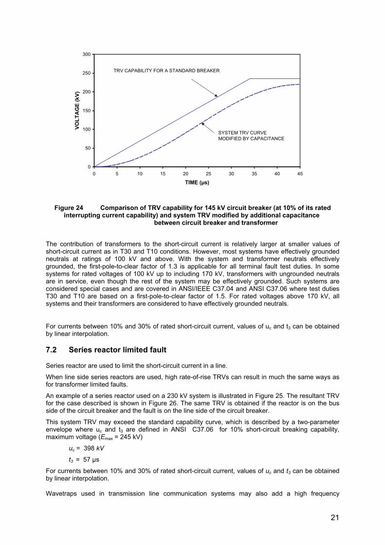
Figure 24 Comparison of TRV capability for 145 kV circuit breaker (at 10% of its ratedinterrupting current capability) and system TRV modified by additional capacitance

between circuit breaker and transformer

The contribution of transformers to the short-circuit current is relatively larger at smaller values ofshort-circuit current as in T30 and T10 conditions. However, most systems have effectively groundedneutrals at ratings of 100 kV and above. With the system and transformer neutrals effectivelygrounded, the first-pole-to-clear factor of 1.3 is applicable for all terminal fault test duties. In somesystems for rated voltages of 100 kV up to including 170 kV, transformers with ungrounded neutralsare in service, even though the rest of the system may be effectively grounded. Such systems areconsidered special cases and are covered in ANSI/IEEE C37.04 and ANSI C37.06 where test dutiesT30 and T10 are based on a first-pole-to-clear factor of 1.5. For rated voltages above 170 kV, allsystems and their transformers are considered to have effectively grounded neutrals.

For currents between 10% and 30% of rated short-circuit current, values of uc and t3 can be obtainedby linear interpolation.

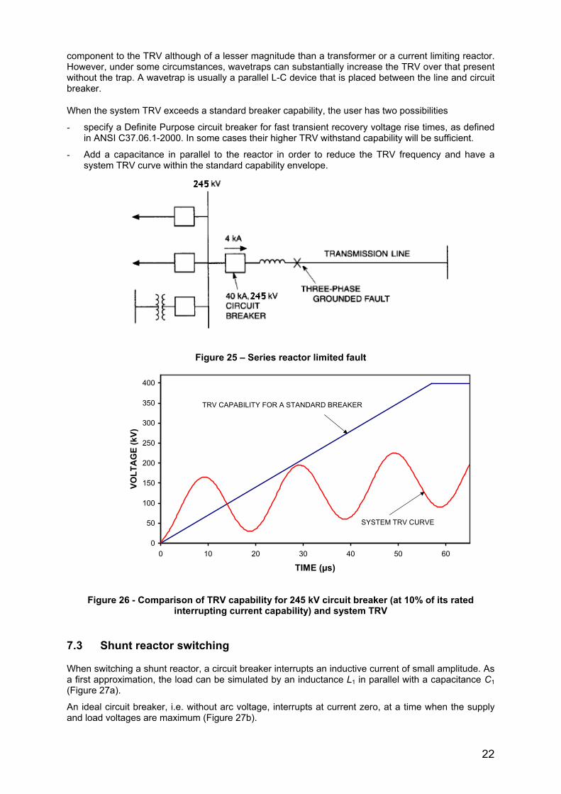
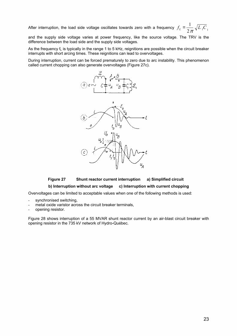
7.2 Series reactor limited fault

Series reactor are used to limit the short-circuit current in a line.

When line side series reactors are used, high rate-of-rise TRVs can result in much the same ways asfor transformer limited faults.

An example of a series reactor used on a 230 kV system is illustrated in Figure 25. The resultant TRVfor the case described is shown in Figure 26. The same TRV is obtained if the reactor is on the busside of the circuit breaker and the fault is on the line side of the circuit breaker.

This system TRV may exceed the standard capability curve, which is described by a two-parameterenvelope where uc and t3 are defined in ANSI C37.06 for 10% short-circuit breaking capability,maximum voltage (Emax = 245 kV)

uc = 398 kV

t3 = 57 µs

For currents between 10% and 30% of rated short-circuit current, values of uc and t3 can be obtainedby linear interpolation.

Wavetraps used in transmission line communication systems may also add a high frequency

0

50

100

150

200

250

300

0 5 10 15 20 25 30 35 40 45

TIME (µs)

VOLT

AG

E (k

V)

SYSTEM TRV CURVEMODIFIED BY CAPACITANCE

TRV CAPABILITY FOR A STANDARD BREAKER

22

component to the TRV although of a lesser magnitude than a transformer or a current limiting reactor.However, under some circumstances, wavetraps can substantially increase the TRV over that presentwithout the trap. A wavetrap is usually a parallel L-C device that is placed between the line and circuitbreaker.

When the system TRV exceeds a standard breaker capability, the user has two possibilities

- specify a Definite Purpose circuit breaker for fast transient recovery voltage rise times, as definedin ANSI C37.06.1-2000. In some cases their higher TRV withstand capability will be sufficient.

- Add a capacitance in parallel to the reactor in order to reduce the TRV frequency and have asystem TRV curve within the standard capability envelope.

Figure 25 – Series reactor limited fault

Figure 26 - Comparison of TRV capability for 245 kV circuit breaker (at 10% of its ratedinterrupting current capability) and system TRV

7.3 Shunt reactor switching

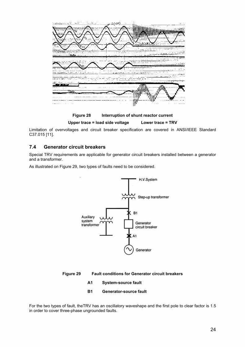
When switching a shunt reactor, a circuit breaker interrupts an inductive current of small amplitude. Asa first approximation, the load can be simulated by an inductance L1 in parallel with a capacitance C1(Figure 27a).

An ideal circuit breaker, i.e. without arc voltage, interrupts at current zero, at a time when the supplyand load voltages are maximum (Figure 27b).

0

50

100

150

200

250

300

350

400

0 10 20 30 40 50 60

TIME (µs)

VOLT

AG

E (k

V)

SYSTEM TRV CURVE

TRV CAPABILITY FOR A STANDARD BREAKER

23

After interruption, the load side voltage oscillates towards zero with a frequency 1121 CLfL π

=

and the supply side voltage varies at power frequency, like the source voltage. The TRV is thedifference between the load side and the supply side voltages.

As the frequency fL is typically in the range 1 to 5 kHz, reignitions are possible when the circuit breakerinterrupts with short arcing times. These reignitions can lead to overvoltages.

During interruption, current can be forced prematurely to zero due to arc instability. This phenomenoncalled current chopping can also generate overvoltages (Figure 27c).

Figure 27 Shunt reactor current interruption a) Simplified circuitb) Interruption without arc voltage c) Interruption with current chopping

Overvoltages can be limited to acceptable values when one of the following methods is used:

- synchronised switching,- metal oxide varistor across the circuit breaker terminals,- opening resistor.

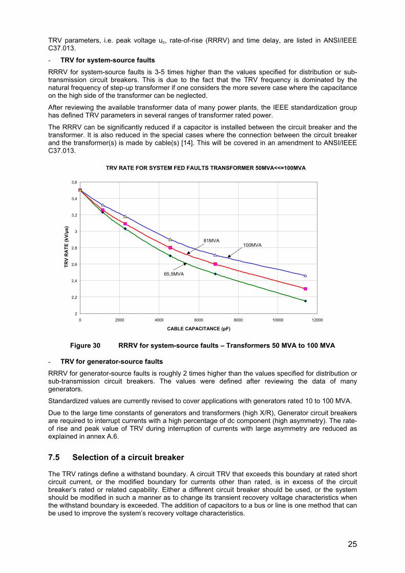
Figure 28 shows interruption of a 55 MVAR shunt reactor current by an air-blast circuit breaker withopening resistor in the 735 kV network of Hydro-Québec.

24

Figure 28 Interruption of shunt reactor currentUpper trace = load side voltage Lower trace = TRV

Limitation of overvoltages and circuit breaker specification are covered in ANSI/IEEE StandardC37.015 [11].

7.4 Generator circuit breakersSpecial TRV requirements are applicable for generator circuit breakers installed between a generatorand a transformer.

As illustrated on Figure 29, two types of faults need to be considered.

Figure 29 Fault conditions for Generator circuit breakers

A1 System-source fault

B1 Generator-source fault

For the two types of fault, theTRV has an oscillatory waveshape and the first pole to clear factor is 1.5in order to cover three-phase ungrounded faults.

25

TRV parameters, i.e. peak voltage uc, rate-of-rise (RRRV) and time delay, are listed in ANSI/IEEEC37.013.

- TRV for system-source faultsRRRV for system-source faults is 3-5 times higher than the values specified for distribution or sub-transmission circuit breakers. This is due to the fact that the TRV frequency is dominated by thenatural frequency of step-up transformer if one considers the more severe case where the capacitanceon the high side of the transformer can be neglected.

After reviewing the available transformer data of many power plants, the IEEE standardization grouphas defined TRV parameters in several ranges of transformer rated power.

The RRRV can be significantly reduced if a capacitor is installed between the circuit breaker and thetransformer. It is also reduced in the special cases where the connection between the circuit breakerand the transformer(s) is made by cable(s) [14]. This will be covered in an amendment to ANSI/IEEEC37.013.

Figure 30 RRRV for system-source faults – Transformers 50 MVA to 100 MVA

- TRV for generator-source faultsRRRV for generator-source faults is roughly 2 times higher than the values specified for distribution orsub-transmission circuit breakers. The values were defined after reviewing the data of manygenerators.

Standardized values are currently revised to cover applications with generators rated 10 to 100 MVA.

Due to the large time constants of generators and transformers (high X/R), Generator circuit breakersare required to interrupt currents with a high percentage of dc component (high asymmetry). The rate-of rise and peak value of TRV during interruption of currents with large asymmetry are reduced asexplained in annex A.6.

7.5 Selection of a circuit breaker

The TRV ratings define a withstand boundary. A circuit TRV that exceeds this boundary at rated shortcircuit current, or the modified boundary for currents other than rated, is in excess of the circuitbreaker’s rated or related capability. Either a different circuit breaker should be used, or the systemshould be modified in such a manner as to change its transient recovery voltage characteristics whenthe withstand boundary is exceeded. The addition of capacitors to a bus or line is one method that canbe used to improve the system’s recovery voltage characteristics.

TRV RATE FOR SYSTEM FED FAULTS TRANSFORMER 50MVA<<=100MVA

2

2,2

2,4

2,6

2,8

3

3,2

3,4

3,6

0 2000 4000 6000 8000 10000 12000

CABLE CAPACITANCE (pF)

TRV

RA

TE (k

V/µs

)

100MVA81MVA

65,5MVA

26

In special cases where the terminal fault TRV capability at 60% or 100% of short-circuit capability ishigher than rated, a breaker with a higher rated interrupting capability could be used (see ANSI/IEEEC37.011).

8 Bibliography

[1] Naef, O., Zimmerman, C. P., and Beehler, J. E., “Proposed Transient Recovery Voltage Ratings forPower Circuit Breakers,” IEEE Transactions on Power Apparatus and Systems, vol. PAS-84, no. 7, pp.580–608, July 1965.

[2] Transient Recovery Voltages on Power Systems (as Related to Circuit Breaker Performance). NewYork: Association of Edison Illuminating Companies, 1963.

[3]] Wagner, C.L., and Smith, H.M., “Analysis of Transient Recovery Voltage (TRV) Rating Concepts,” IEEETransactions, vol. PAS-103, pp. 3354-3363, Nov. 1984.

[4] ANSI C37.06, AC High-Voltage Circuit Breakers Rated on a Symmetrical Current Basis—PreferredRatings and Related Required Capabilities (under revision).

[5] ANSI C37.011, Application Guide for Transient Recovery Voltage for AC High-Voltage CircuitBreakers. (under revision).

[6] ANSI C37.06.1-2000, Guide for High-Voltage Circuit Breakers Rated on a Symmetrical Current BasisDesignated “Definite Purpose for Fast Transient Recovery Voltage Rise Times”.

[7] ANSI/IEEE Std C37.04, IEEE Standard Rating Structure for AC High-Voltage Circuit Breakers (underrevision).

[8] ANSI/IEEE Std C37.09, IEEE Standard Test Procedure for AC High-Voltage Circuit Breakers (underrevision).

[9] ANSI/IEEE Std C37.013, IEEE Standard for AC High-Voltage Generator Circuit Breakers Rated on aSymmetrical Current Basis.

[10] A.Greenwood, “Electrical Transients in Power Systems”, Second Edition, John Wiley & Sons Inc,1991.

[11] ANSI/IEEE Std C37.015, IEEE Application Guide for Shunt Reactor Switching.

[12] Harner R.and Rodriguez J., “Transient Recovery Voltages Associated with Power System, Three-phasetransformer secondary faults”, IEEE Transactions, vol. PAS-91, pp. 1887–1896, Sept./Oct. 1972.

[13] Colclaser R.G. and Buettner D.E., “The traveling wave Approach to Transient Recovery Voltage”,IEEE Transactions on Power Apparatus and Systems, vol. PAS-88, N°7, July 1969.

[14] Dufournet D. and Montillet G., “Transient Recovery Voltages Requirements for System Source FaultInterrupting by Small Generator Circuit Breakers”, IEEE Transactions on Power Delivery, Vol.17, N°2,April 2002.

[15] Griscom S.B., Sauter D.M. and Ellis H.M., “Transient Recovery Voltages on Power Systems – Part II-Practical Methods of Determination”, AIEE Transactions, Vol. 77, August 1958, pp 592-606.

[16] Hedman, D. E., and Lambert, S. R., “Power Circuit Breaker Transient Recovery Voltages,” IEEETransactions on Power Apparatus and Systems, vol. PAS-95, pp. 197–207, Jan./Feb. 1976.

27

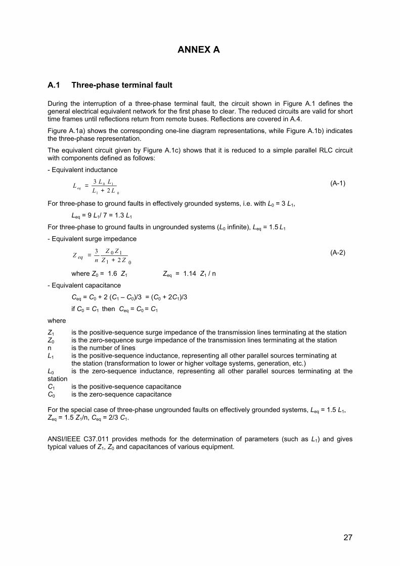
ANNEX A

A.1 Three-phase terminal fault

During the interruption of a three-phase terminal fault, the circuit shown in Figure A.1 defines thegeneral electrical equivalent network for the first phase to clear. The reduced circuits are valid for shorttime frames until reflections return from remote buses. Reflections are covered in A.4.

Figure A.1a) shows the corresponding one-line diagram representations, while Figure A.1b) indicatesthe three-phase representation.

The equivalent circuit given by Figure A.1c) shows that it is reduced to a simple parallel RLC circuitwith components defined as follows:

- Equivalent inductance

01

10

23

LLLLL eq +

= (A-1)

For three-phase to ground faults in effectively grounded systems, i.e. with L0 = 3 L1,

Leq = 9 L1/ 7 = 1.3 L1

For three-phase to ground faults in ungrounded systems (L0 infinite), Leq = 1.5 L1

- Equivalent surge impedance

01

102

3ZZ

ZZn

Z eq += (A-2)

where Z0 = 1.6 Z1 Zeq = 1.14 Z1 / n

- Equivalent capacitance

Ceq = C0 + 2 (C1 – C0)/3 = (C0 + 2C1)/3

if C0 = C1 then Ceq = C0 = C1

where

Z1 is the positive-sequence surge impedance of the transmission lines terminating at the stationZ0 is the zero-sequence surge impedance of the transmission lines terminating at the stationn is the number of linesL1 is the positive-sequence inductance, representing all other parallel sources terminating at

the station (transformation to lower or higher voltage systems, generation, etc.)L0 is the zero-sequence inductance, representing all other parallel sources terminating at thestation C1 is the positive-sequence capacitanceC0 is the zero-sequence capacitance

For the special case of three-phase ungrounded faults on effectively grounded systems, Leq = 1.5 L1, Zeq = 1.5 Z1/n, Ceq = 2/3 C1.

ANSI/IEEE C37.011 provides methods for the determination of parameters (such as L1) and givestypical values of Z1, Z0 and capacitances of various equipment.

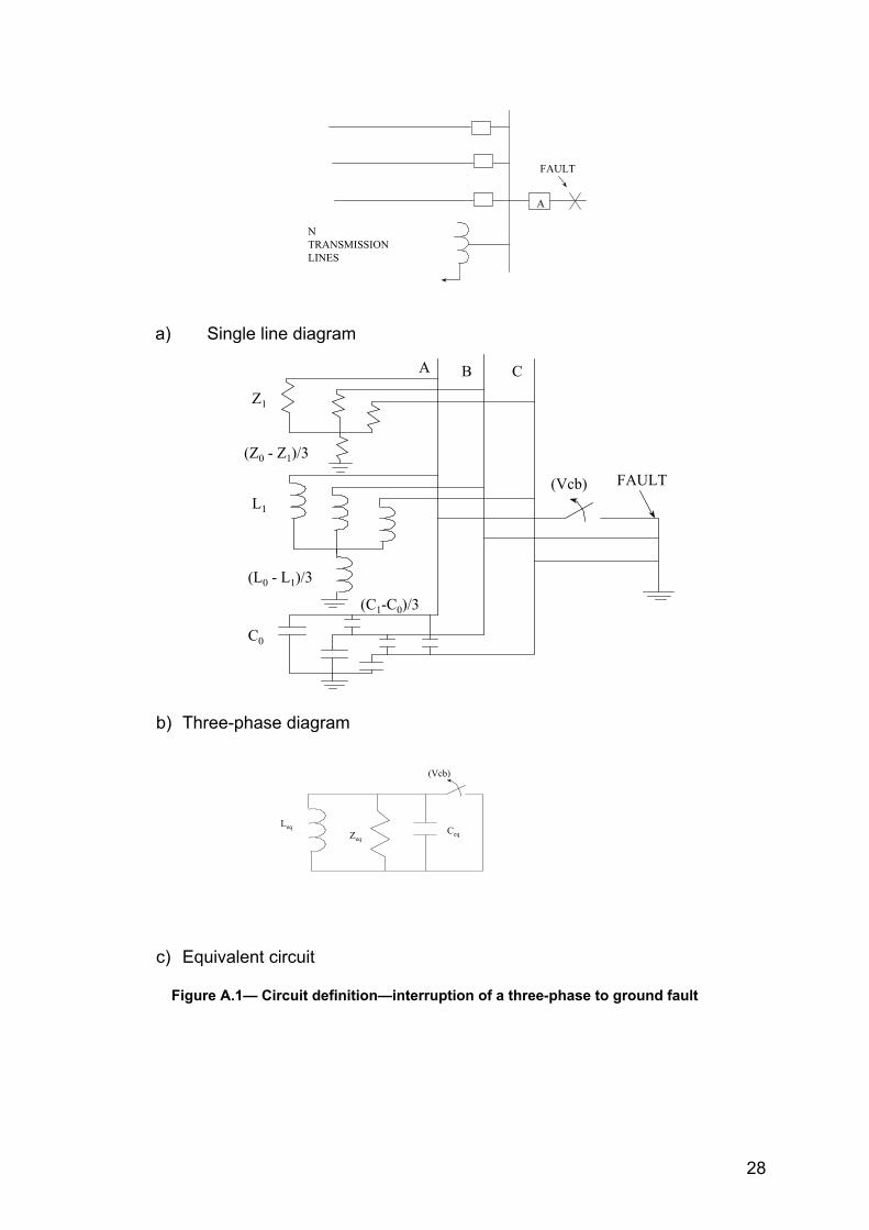
28

A

NTRANSMISSIONLINES

FAULT

a) Single line diagram

FAULT

C0

(L0 - L1)/3

L1

Z1

A B C

(Vcb)

(Z0 - Z1)/3

(C1-C0)/3

b) Three-phase diagram

ZeqCeq

(Vcb)

Leq

c) Equivalent circuit

Figure A.1— Circuit definition—interruption of a three-phase to ground fault

29

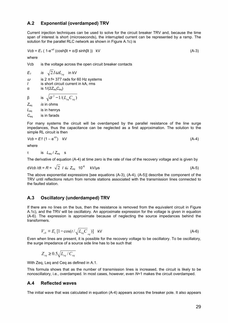
A.2 Exponential (overdamped) TRV

Current injection techniques can be used to solve for the circuit breaker TRV and, because the timespan of interest is short (microseconds), the interrupted current can be represented by a ramp. Thesolution for the parallel RLC network as shown in Figure A.1c) is

Vcb = E1 ( 1-e-αt (coshβt + α/β sinhβt )) kV (A-3)

where

Vcb is the voltage across the open circuit breaker contacts

E1 is eqLIω2 in kV

ω is 2 π f= 377 rads for 60 Hz systems I is short circuit current in kA, rmsα is 1/(2ZeqCeq)

β is )/(12eqeqCL−α

Zeq is in ohmsLeq is in henrysCeq is in farads

For many systems the circuit will be overdamped by the parallel resistance of the line surgeimpedances, thus the capacitance can be neglected as a first approximation. The solution to thesimple RL circuit is then

Vcb = E1 (1 – e-t/τ) kV (A-4)

where

τ is Leq / Zeq s

The derivative of equation (A-4) at time zero is the rate of rise of the recovery voltage and is given by

dVcb /dt = R = 2 I ω Zeq 10-6 kV/µs (A-5)

The above exponential expressions [see equations (A-3), (A-4), (A-5)] describe the component of theTRV until reflections return from remote stations associated with the transmission lines connected tothe faulted station.

A.3 Oscillatory (underdamped) TRV

If there are no lines on the bus, then the resistance is removed from the equivalent circuit in FigureA.1c), and the TRV will be oscillatory. An approximate expression for the voltage is given in equation(A-6). The expression is approximate because of neglecting the source impedances behind thetransformers.

)]/cos(1[1 eqeqcb CLtEV −= kV (A-6)

Even when lines are present, it is possible for the recovery voltage to be oscillatory. To be oscillatory,the surge impedance of a source side line has to be such that

eqeqeq CLZ /5.0≥

With Zeq, Leq and Ceq as defined in A.1.

This formula shows that as the number of transmission lines is increased, the circuit is likely to benonoscillatory, i.e., overdamped. In most cases, however, even N=1 makes the circuit overdamped.

A.4 Reflected waves

The initial wave that was calculated in equation (A-4) appears across the breaker pole. It also appears

30

as traveling waves on each of the transmission lines. When one of these waves reaches adiscontinuity on the line such as another bus or a transformer termination, a reflected wave isproduced, which travels back towards the faulted bus. The time for a wave to go out and back to adiscontinuity is

klT µ65.6= µs (A-7)

l is the distance to the first discontinuity (in kilometer)

µ is the magnetic permeability

k is the dielectric constant

for overhead lines

kµ = 1.0 and Z1 about 400 ohms (less for bundled conductor 250<Z1<350)

for cables, typically

Paper insulated fluid filled k = 4 , µ = 1.0 and kµ = 2

PPP insulated fluid filled or EPR k = 3 , µ = 1.0 and kµ = 1.73

Polyethylene k = 2.3 , µ = 1.0 and kµ = 1.52

Cable Surge Impedance (ohms) 20 < Z1 < 50

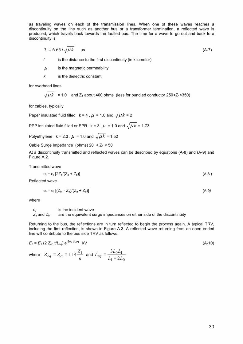
At a discontinuity transmitted and reflected waves can be described by equations (A-8) and (A-9) andFigure A.2.

Transmitted wave

et = ei [2Zb/(Za + Zb)] (A-8 )

Reflected wave

er = ei [(Zb - Za)/(Za + Zb)] (A-9)

where

ei is the incident waveZa and Zb are the equivalent surge impedances on either side of the discontinuity

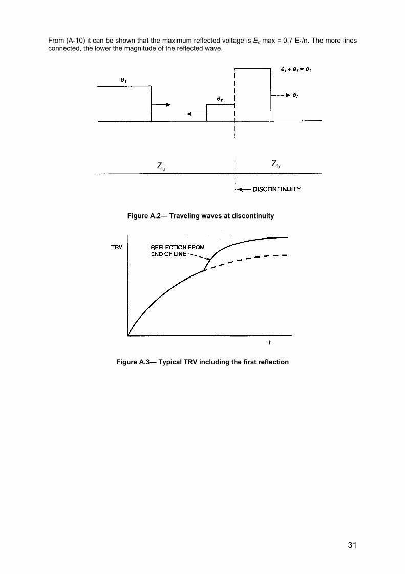
Returning to the bus, the reflections are in turn reflected to begin the process again. A typical TRV,including the first reflection, is shown in Figure A.3. A reflected wave returning from an open endedline will contribute to the bus side TRV as follows:

Erl = E1 (2 Zeq t/Leq) e-Zeq t/Leq kV (A-10)

wheren

ZZZ aeq114.1== and

01

102

3LL

LLLeq +

=

31

From (A-10) it can be shown that the maximum reflected voltage is Erl max = 0.7 E1/n. The more linesconnected, the lower the magnitude of the reflected wave.

Figure A.2— Traveling waves at discontinuity

Figure A.3— Typical TRV including the first reflection

ZaZb

32

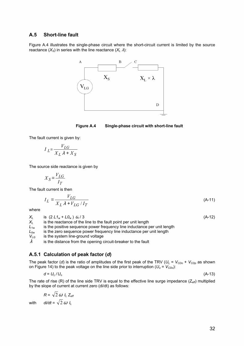
A.5 Short-line fault

Figure A.4 illustrates the single-phase circuit where the short-circuit current is limited by the sourcereactance (XS) in series with the line reactance (XL λ):

Figure A.4 Single-phase circuit with short-line fault

The fault current is given by:

SL

LGL XX

VI

+=

λ

The source side reactance is given by

T

LGS I

VX =

The fault current is then

TLGL

LGL IVX

VI

/+=

λ(A-11)

where

XL is (2 L1w + L0w ) ω / 3 (A-12)XL is the reactance of the line to the fault point per unit lengthL1w is the positive sequence power frequency line inductance per unit lengthL0w is the zero sequence power frequency line inductance per unit lengthVLG is the system line-ground voltageλ is the distance from the opening circuit-breaker to the fault

A.5.1 Calculation of peak factor (d)The peak factor (d) is the ratio of amplitudes of the first peak of the TRV (UL = VCDo + VCDp as shownon Figure 14) to the peak voltage on the line side prior to interruption (Uo = VCDo):

d = UL / Uo (A-13)

The rate of rise (R) of the line side TRV is equal to the effective line surge impedance (Zeff) multipliedby the slope of current at current zero (di/dt) as follows:

R = ω2 IL Zeff

with di/dt = ω2 IL

33

The time to the first peak UL is equal to two times the travel time from the circuit breaker to the faultpoint (time necessary for the traveling wave to reach the fault and be reflected back to the circuitbreaker) : 2 λ / v = tL

whereλ is the distance from the opening circuit-breaker to the fault v is the velocity of light

It follows that the first peak of the line side TRV is given by :

UL = Zeff di/dt 2 λ / v (A-14)Uo = XL λ IL 2 (A-15)

From (A-13), (A-14) and (A-15):

vXZ

dL

effω2= (A-16)

where

XL = (2 L1w + L0w ) ω / 3

Zeff = (2Z1 + Z0)/3 (A-17)

111 / CLZ = (A-18)

11/1 CLv = (A-19)Z1 = positive sequence surge impedanceZ0 = zero sequence surge impedanceL1 = high-frequency positive sequence line inductance per unit lengthC1 = high-frequency positive sequence line capacitance per unit length

The effective surge impedance Zeff is influenced by bundle and tower configuration.

From (A-18) and (A-19):

Z1 / v = L1 (A-20)

From (A-16), (A-17), (A-18) and (A-20):

ωω

ωω

3)2)(3(

)2(2011

101

LLZLZZd

++=

or )2(

)/2(201

110

ωω LLLZZd

++= (A-21)

If the high-frequency inductance L1 is equal to the power frequency inductance of the line L1w, formula(A-21) simplifies to:

)/2()/2(2

10

10

ωω LLZZd

++= (A-22)

if L0w/L1w ≈ 3 is assumed for high-voltage networks:

)/2(4.0 10 ZZd += (A-23)

In practice the high frequency inductance L1 is lower than the power frequency value L1w., and losseswhich are always present have been neglected in the calculation. For these reasons the peak factorvalue obtained by (A-23) is conservative.

As the ratio Z0/Z1 is always lower than 2 for HV networks, 72.5 kV to 550 kV, values of the peak factor(d) is equal or lower than 1.6. Therefore the standardised value of 1.6 is conservative.

Using (A-17) and (A-23) the peak factor is

34

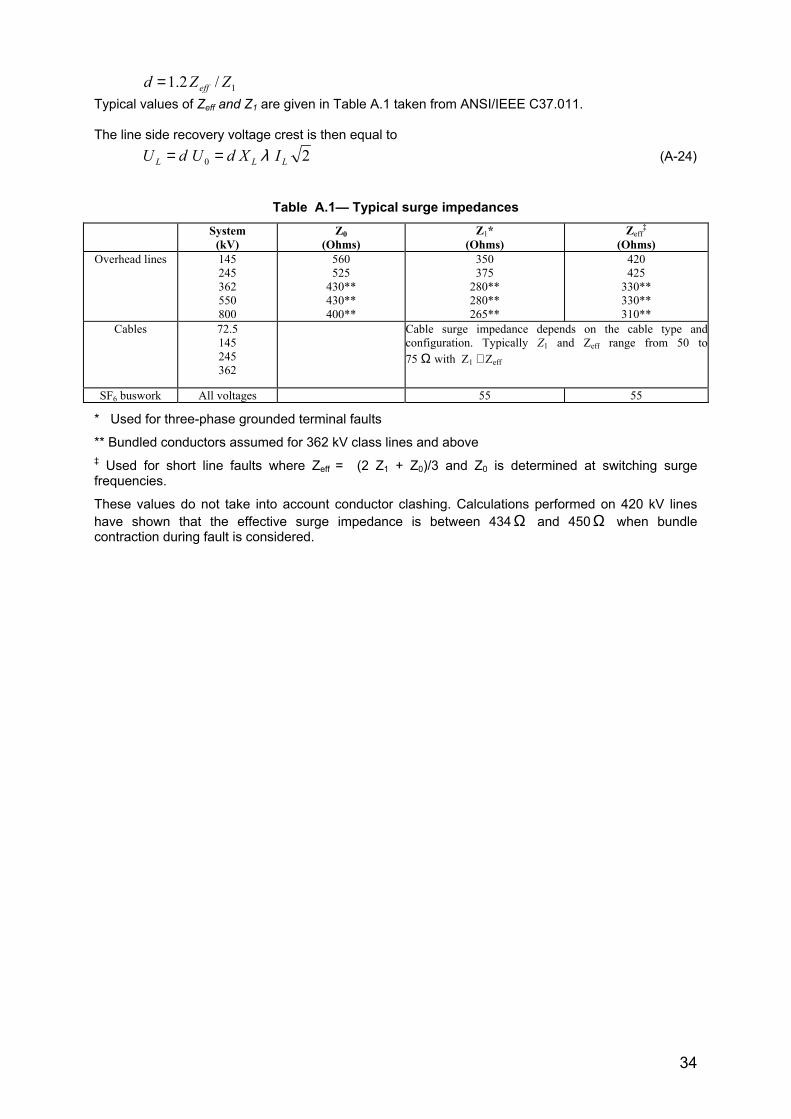
1/2.1 ZZd eff=Typical values of Zeff and Z1 are given in Table A.1 taken from ANSI/IEEE C37.011.

The line side recovery voltage crest is then equal to20 LLL IXdUdU λ== (A-24)

Table A.1— Typical surge impedancesSystem(kV)

Z0(Ohms)

Z1*(Ohms)

Zeff‡

(Ohms)Overhead lines 145

245362550800

560525

430**430**400**

350375

280**280**265**

420425

330**330**310**

Cables 72.5145245362

Cable surge impedance depends on the cable type andconfiguration. Typically Z1 and Zeff range from 50 to75 Ω with Z1 ≅ Zeff

SF6 buswork All voltages 55 55

* Used for three-phase grounded terminal faults

** Bundled conductors assumed for 362 kV class lines and above‡ Used for short line faults where Zeff = (2 Z1 + Z0)/3 and Z0 is determined at switching surgefrequencies.

These values do not take into account conductor clashing. Calculations performed on 420 kV lineshave shown that the effective surge impedance is between 434 Ω and 450 Ω when bundlecontraction during fault is considered.

35

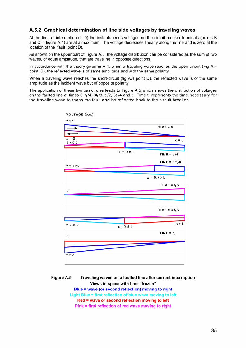
A.5.2 Graphical determination of line side voltages by traveling wavesAt the time of interruption (t= 0) the instantaneous voltages on the circuit breaker terminals (points Band C in figure A.4) are at a maximum. The voltage decreases linearly along the line and is zero at thelocation of the fault (point D).

As shown on the upper part of Figure A.5, the voltage distribution can be considered as the sum of twowaves, of equal amplitude, that are traveling in opposite directions.

In accordance with the theory given in A.4, when a traveling wave reaches the open circuit (Fig A.4point B), the reflected wave is of same amplitude and with the same polarity.

When a traveling wave reaches the short-circuit (fig A.4 point D), the reflected wave is of the sameamplitude as the incident wave but of opposite polarity.

The application of these two basic rules leads to Figure A.5 which shows the distribution of voltageson the faulted line at times 0, tL/4, 3tL/8, tL/2, 3tL/4 and tL. Time tL represents the time necessary forthe traveling wave to reach the fault and be reflected back to the circuit breaker.

Figure A.5 Traveling waves on a faulted line after current interruptionViews in space with time “frozen”

Blue = wave (or second reflection) moving to rightLight Blue = first reflection of blue wave moving to left

Red = wave or second reflection moving to leftPink = first reflection of red wave moving to right

x = Lx = 0

x = 0.5 L

VOLTAGE (p.u.)

2 x 0.5

2 x 0.25

x = 0.75 L

0

2 x -0.5 x= 0.5 Lx= L

2 x 1

2 x -1

TIME = 0

TIME = tL/4

TIME = 3 tL/8

TIME = tL/2

TIME = 3 tL/2

TIME = tL0

36

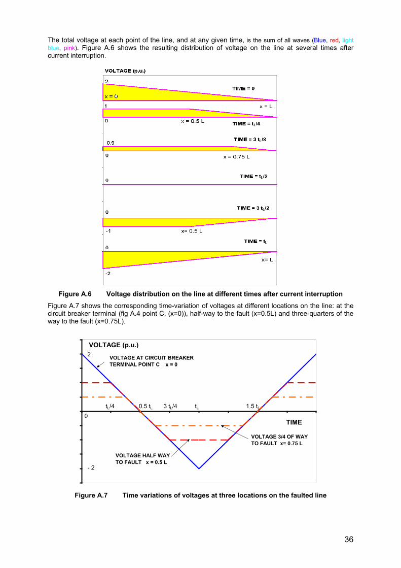
The total voltage at each point of the line, and at any given time, is the sum of all waves (Blue, red, lightblue, pink). Figure A.6 shows the resulting distribution of voltage on the line at several times aftercurrent interruption.

Figure A.6 Voltage distribution on the line at different times after current interruptionFigure A.7 shows the corresponding time-variation of voltages at different locations on the line: at thecircuit breaker terminal (fig A.4 point C, (x=0)), half-way to the fault (x=0.5L) and three-quarters of theway to the fault (x=0.75L).

Figure A.7 Time variations of voltages at three locations on the faulted line

VOLTAGE AT CIRCUIT BREAKERTERMINAL POINT C x = 0

VOLTAGE HALF WAYTO FAULT x = 0.5 L

VOLTAGE 3/4 OF WAY TO FAULT x= 0.75 L

TIME

VOLTAGE (p.u.)

0

2

- 2

tL0.5 tL tL/4 3 tL/4 1.5 tL

37

The voltage at the circuit breaker terminal has the well known triangular waveshape. If the voltage onthe supply side terminal (figure A.4 point B) is assumed to be constant, since the TRV frequency onthe supply side is very low when compared with the line side TRV, the TRV across the circuit breakerterminals has the waveshape shown on figure 13. The forgoing treatment of short line fault TRV hasignored the effects of damping. Damping occurs due to line losses, and imperfect reflections. Thefault is not usually a complete short circuit. The open circuit breaker is not an infinite impedance.(especially in the first microsecond) Damping will give rise to lower peak factors than those used instandards.

A.5.3 Calculation of Short-line fault quantities

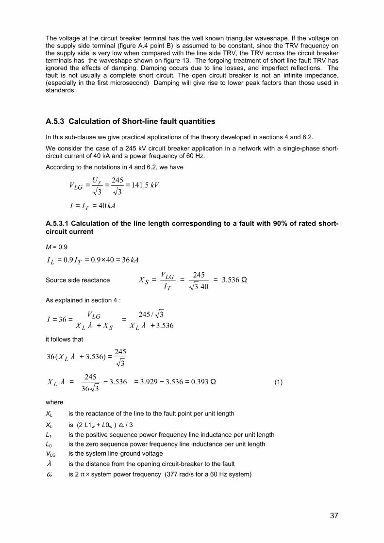
In this sub-clause we give practical applications of the theory developed in sections 4 and 6.2.

We consider the case of a 245 kV circuit breaker application in a network with a single-phase short-circuit current of 40 kA and a power frequency of 60 Hz.

According to the notations in 4 and 6.2, we have

kVU

V rLG 5.141

3245

3===

kAII T 40==

A.5.3.1 Calculation of the line length corresponding to a fault with 90% of rated short-circuit current

M = 0.9

kAII TL 36409.09.0 =×==

Source side reactance Ω=== 536.3403

245

T

LGS I

VX

As explained in section 4 :

536.33/24536

+=

+==

λλ LSL

LGXXX

VI

it follows that

3245)536.3(36 =+λLX

Ω=−=−= 393.0536.3929.3536.3336

245λLX (1)

where

XL is the reactance of the line to the fault point per unit length

XL is (2 L1w + L0w ) ω / 3L1 is the positive sequence power frequency line inductance per unit lengthL0 is the zero sequence power frequency line inductance per unit lengthVLG is the system line-ground voltageλ is the distance from the opening circuit-breaker to the fault ω is 2 π × system power frequency (377 rad/s for a 60 Hz system)

38

32

3)2( 01

01XX

LLX L+

=+= ω

with

kmLX /5.011 Ω== ω

kmLX /2.100 Ω== ω

kmX L /32.2

32.15.02 Ω=+×= (2)

From (1) and (2)

km536.02.2393.03

3/2.2393.0 =×==λ

A.5.3.2 Calculation of the fault current corresponding to a length of faulted lineIn this second example of calculation we consider the case of a fault 1.5 km away on the line.

Ω== 1.15.132.2λLX

kAI 5.30636.4

45.141536.31.1

3/245 ==+

=

It follows that 76.040

5.30 ==M

The fault current is 76% of the maximum (single-phase) short-circuit current.

A.5.3.3 Calculation of the first peak of TRV In the example A.5.3.1, M is 0.9 i.e. the fault current is 90% of the rated short-circuit current.

a) Contribution of the line side voltage (e)

kVe

UrMde

322453/21.06.1

3/2)1(

=×××=

−=

b) Contribution of source side voltage )( Se

As explained in sub-clause 6.2, the contribution of the source side voltage is:

)2(2 −= LS TMxe (3)

The time to peak LT is determined as follows:

µskVµskVR

IMZR

L

L

/64.8409.024.0/10409.04503772

26

=××=××××=

=−

ω

µsReTL

L 7.364.8

32 === (4)

39

From (3) and (4):

kVeS 3)27.3(9.02 =−××=

The first peak of TRV across the circuit breaker terminals is then

kVeee ST 35332 =+=+=

The rate-of-rise of recovery voltage is µskVTeRRRV

L

T /46.97.3

35 ===

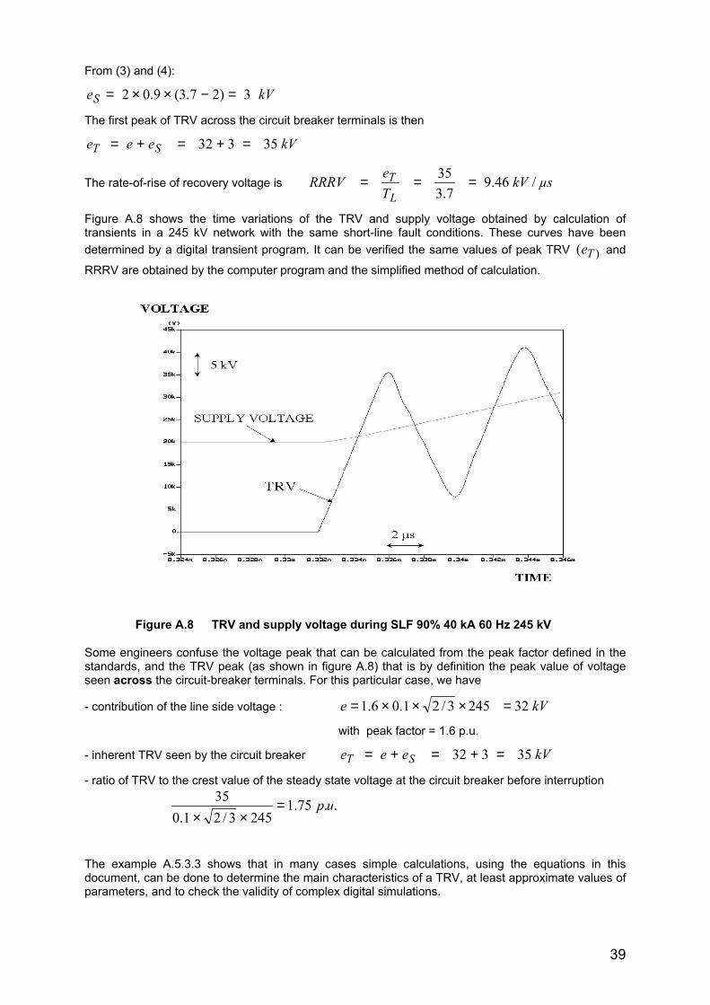
Figure A.8 shows the time variations of the TRV and supply voltage obtained by calculation oftransients in a 245 kV network with the same short-line fault conditions. These curves have beendetermined by a digital transient program. It can be verified the same values of peak TRV )( Te and

RRRV are obtained by the computer program and the simplified method of calculation.

Figure A.8 TRV and supply voltage during SLF 90% 40 kA 60 Hz 245 kV

Some engineers confuse the voltage peak that can be calculated from the peak factor defined in thestandards, and the TRV peak (as shown in figure A.8) that is by definition the peak value of voltageseen across the circuit-breaker terminals. For this particular case, we have

- contribution of the line side voltage : kVe 322453/21.06.1 =×××=

with peak factor = 1.6 p.u.

- inherent TRV seen by the circuit breaker kVeee ST 35332 =+=+=

- ratio of TRV to the crest value of the steady state voltage at the circuit breaker before interruption

..75.12453/21.0

35 up=××

The example A.5.3.3 shows that in many cases simple calculations, using the equations in thisdocument, can be done to determine the main characteristics of a TRV, at least approximate values ofparameters, and to check the validity of complex digital simulations.

40

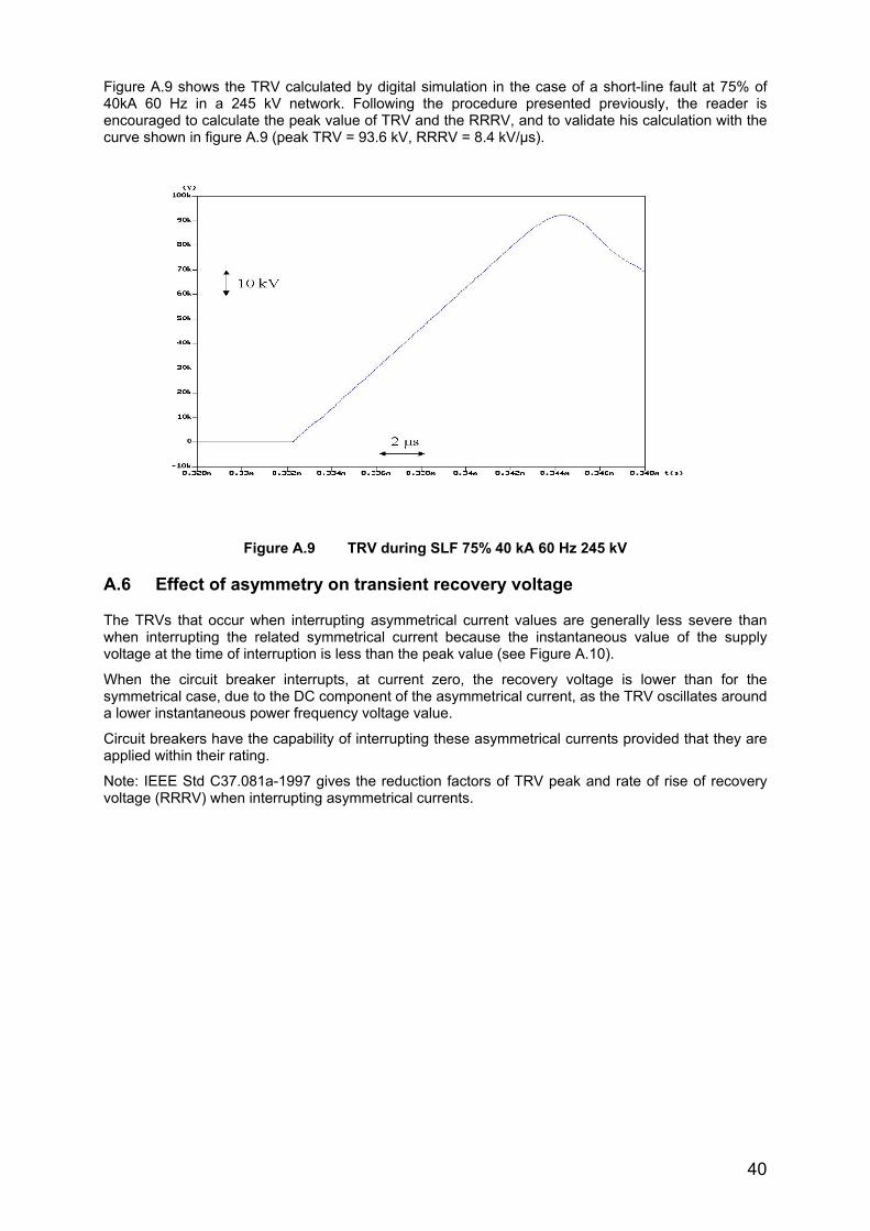
Figure A.9 shows the TRV calculated by digital simulation in the case of a short-line fault at 75% of40kA 60 Hz in a 245 kV network. Following the procedure presented previously, the reader isencouraged to calculate the peak value of TRV and the RRRV, and to validate his calculation with thecurve shown in figure A.9 (peak TRV = 93.6 kV, RRRV = 8.4 kV/µs).

Figure A.9 TRV during SLF 75% 40 kA 60 Hz 245 kV

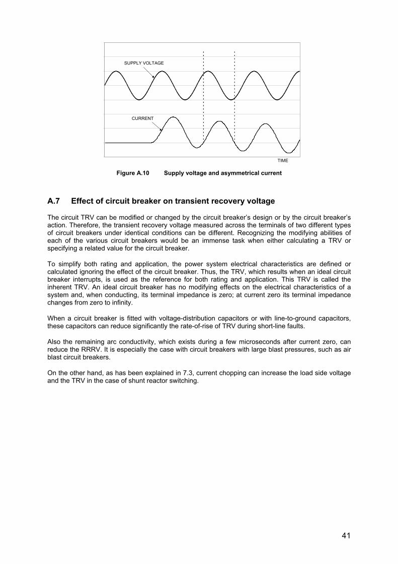
A.6 Effect of asymmetry on transient recovery voltage

The TRVs that occur when interrupting asymmetrical current values are generally less severe thanwhen interrupting the related symmetrical current because the instantaneous value of the supplyvoltage at the time of interruption is less than the peak value (see Figure A.10).

When the circuit breaker interrupts, at current zero, the recovery voltage is lower than for thesymmetrical case, due to the DC component of the asymmetrical current, as the TRV oscillates arounda lower instantaneous power frequency voltage value.

Circuit breakers have the capability of interrupting these asymmetrical currents provided that they areapplied within their rating.

Note: IEEE Std C37.081a-1997 gives the reduction factors of TRV peak and rate of rise of recoveryvoltage (RRRV) when interrupting asymmetrical currents.

41

Figure A.10 Supply voltage and asymmetrical current

A.7 Effect of circuit breaker on transient recovery voltage

The circuit TRV can be modified or changed by the circuit breaker’s design or by the circuit breaker’saction. Therefore, the transient recovery voltage measured across the terminals of two different typesof circuit breakers under identical conditions can be different. Recognizing the modifying abilities ofeach of the various circuit breakers would be an immense task when either calculating a TRV orspecifying a related value for the circuit breaker.

To simplify both rating and application, the power system electrical characteristics are defined orcalculated ignoring the effect of the circuit breaker. Thus, the TRV, which results when an ideal circuitbreaker interrupts, is used as the reference for both rating and application. This TRV is called theinherent TRV. An ideal circuit breaker has no modifying effects on the electrical characteristics of asystem and, when conducting, its terminal impedance is zero; at current zero its terminal impedancechanges from zero to infinity.

When a circuit breaker is fitted with voltage-distribution capacitors or with line-to-ground capacitors,these capacitors can reduce significantly the rate-of-rise of TRV during short-line faults.

Also the remaining arc conductivity, which exists during a few microseconds after current zero, canreduce the RRRV. It is especially the case with circuit breakers with large blast pressures, such as airblast circuit breakers.

On the other hand, as has been explained in 7.3, current chopping can increase the load side voltageand the TRV in the case of shunt reactor switching.

TIME

CURRENT

SUPPLY VOLTAGE