transmission error in spur gears: static and dynamic...
TRANSCRIPT
Transmission Error in Spur Gears: Static and Dynamic
Finite-Element Modeling and Design Optimization
By
Raul Tharmakulasingam
BEng. MSc. (Eng)
Submitted in accordance with the requirements for the degree of Doctor of Philosophy
School of Engineering and Design
Brunel University
United Kingdom
October 2009

~ II ~
ACKNOWLEDGEMENTS
“Success is sweet: the sweeter if long delayed and attained through manifold struggles
and defeats.”
I would like to take this opportunity to thank everyone who has helped me in my pursuit
of success in my PhD. Firstly; I would like to thank my supervisor Dr. Giulio Alfano for
helping me shape my research and motivating me at the right times with a timely
reminder of how much we have achieved. I would also like to Dr Mark Atherton for
bringing a fresh perspective to everything we did during the research, and always
providing a kind ear and an objective view to all our problems. I am also very grateful to
Prof. Luiz Wrobel for providing me with the opportunity to undertake my PhD research,
and also helping me with my numerous problems while carrying out my research. To the
colleagues who helped me with moments of respite during a hard day’s work, inspiration
by example, and lasting friendships, I thank you from the bottom of my heart and look
forward to keeping in touch.
My family who have endured my worst and celebrated my best of times during my PhD
also receive a heartfelt embrace and acknowledgement for everything they have done for
me. My dear friends who constantly reminded me of my duty to hand in my Thesis by
the incessant question “Have you submitted yet?”. I thank you for the motivation and the
celebrations afterwards!
Finally, to the one person who understands me better than I do myself, Jonit, you are my
life, my love and my soul. I could not have completed my PhD without you. You helped
me in so many ways that I cannot begin to describe them on this finite piece of paper. I
look forward to being there for you when you write up your PhD Thesis, and help you in
every way I can. I just want to thank you and let you know that I will always remember
and be there for you, always…
~ III ~
ABSTRACT
The gear noise problem that widely occurs in power transmission systems is typically
characterised by one or more high amplitude acoustic signals. The noise originates from
the vibration of the gear pair system caused by transmission error excitation that arises
from tooth profile errors, misalignment and tooth deflections. This work aims to further
research the effect of tooth profile modifications on the transmission error of gear pairs.
A spur gear pair was modelled using finite elements, and the gear mesh was simulated
and analysed under static conditions. The results obtained were used to study the effect
of intentional tooth profile modifications on the transmission error of the gear pair. A
detailed parametric study, involving development of an optimisation algorithm to design
the tooth modifications, was performed to quantify the changes in the transmission error
as a function of tooth profile modification parameters as compared to an unmodified gear
pair baseline. The work also investigates the main differences between the static and
dynamic transmission error generated during the meshing of a spur gear pair model. A
combination of Finite-Element Analysis, hybrid numerical/analytical methodology and
optimisation algorithms were used to scrutinise the dynamic behaviour of the gear pairs
under various operating conditions.

~ IV ~
PUBLICATIONS
Static and dynamic transmission error of spur gear pair, R. Tharmakulasingam, G.
Alfano, M. Atherton, Submitted to Journal of Sound and Vibration: (July 2010).
Reduction of gear pair transmission error with tooth profile modification, R.
Tharmakulasingam, G. Alfano, M. Atherton, Proceedings of International conference
on Sound and Vibration: (September 2008).
~ V ~
Table of Contents
1. Introduction ............................................................................................................... 1
1.1 Background .......................................................................................................... 1
1.2 Scope and objectives ............................................................................................ 6
1.2.1 Comparison between STE and DTE ........................................................... 7
1.2.2 Full non-linear dynamic finite-element analyses of gear pair interaction... 7
1.2.3 Validation of our FE model with the Hybrid Numerical model ................. 8
1.2.4 Application of the automated profile modification tool to reduce TE ........ 8
1.3 Outline of Thesis .................................................................................................. 9
2. Fundamentals of gear design ................................................................................. 12
2.1 Introduction ............................................................................................................ 12
2.2 Types of gears ........................................................................................................ 13
2.2.1 Spur gears ....................................................................................................... 13
2.2.2 Helical gears ................................................................................................... 14
2.2.3 Bevel gears ..................................................................................................... 15
2.2.4 Worm gears ................................................................................................... 16
2.3 Gear selection criteria ............................................................................................ 17
2.4 Spur gear nomenclature ......................................................................................... 18
2.5 Velocity ratio .......................................................................................................... 20
2.6 Conjugate action..................................................................................................... 21
2.7 Gear tooth profile ................................................................................................... 22
2.8 Standardisation of gears ......................................................................................... 24
2.9 Contact ratio of gears ............................................................................................. 25
2.10 Interference in gears ............................................................................................. 27
2.11 Manufacturing of gear teeth ................................................................................. 28
2.11.1 Milling .......................................................................................................... 30
2.11.2 Shaping ......................................................................................................... 30
2.11.3 Hobbing ........................................................................................................ 30
2.12 Spur gears ............................................................................................................. 31
3. Literature review ..................................................................................................... 34
3.1 Introduction ............................................................................................................ 34
3.2 Engine related gear noise ....................................................................................... 34
3.3 Main types of gear noise ........................................................................................ 35
3.3.1 Gear rattle in gear transmissions .................................................................... 36
3.3.2 Gear whine in gear dynamics ......................................................................... 37
~ VI ~
3.4 General gear noise research ................................................................................... 40
3.5 Introduction to transmission error .......................................................................... 42
3.5.1 Sources of transmission error ......................................................................... 43
3.5.2 Types of transmission error ............................................................................ 47
3.5.2.1 Manufacturing transmission error ........................................................... 47
3.5.2.2 Static transmission error .......................................................................... 48
3.5.2.3 Kinematic transmission error .................................................................. 48
3.5.2.4 Dynamic transmission error .................................................................... 49
3.6 Methods to estimate transmission error ................................................................. 49
3.7 Mesh stiffness modelling ....................................................................................... 51
3.8 Gear dynamic modelling ......................................................................................... 52
3.9 Non-linear finite element analysis of gear pairs .................................................... 53
3.10 Optimisation of gears ........................................................................................... 56
3.10.1 Optimisation criteria .................................................................................... 56
4. Spur Gear methodology and data validation ....................................................... 58
4.1 Introduction ............................................................................................................ 58
4.2 Lewis’s formula for gear strength calculation ....................................................... 58
4.3 Modified Lewis formula ........................................................................................ 63
4.4 Dynamic factor, Kv................................................................................................. 63
4.5 Overload factor, KO ................................................................................................ 64
4.6 Size factor, KS ........................................................................................................ 65
4.7 Load distribution factor, KH ................................................................................... 65
4.8 Rim thickness factor, KB ........................................................................................ 66
4.9 Expressing the load as a function of the transmitted power................................... 67
4.10 Evaluation of the contact stress ............................................................................ 68
4.11 Gear design using the expressions for bending and contact stress....................... 68
5. Automated spur gear profile generation methodology using Python scripts in
Abaqus .............................................................................................................................. 71
5.1 Design of spur gear geometry ................................................................................ 72
5.2 Finite element analysis in Abaqus.......................................................................... 83
5.3 Analysis steps ......................................................................................................... 85
5.3.1 General Analysis ............................................................................................ 85
5.3.1.1 Material nonlinearity ............................................................................... 85
5.3.1.2 Geometric nonlinearity ........................................................................... 86
5.3.1.3 Boundary nonlinearity ............................................................................. 86
5.3.2 Linear perturbation analysis step ................................................................... 86
5.3.3 Direct linear equation solver .......................................................................... 87

~ VII ~
5.3.4 Iterative linear equation solver ....................................................................... 87
5.3.5 Dynamic analysis ........................................................................................... 88
5.3.5.1 Explicit analysis ...................................................................................... 88
5.3.5.2 Implicit analysis ...................................................................................... 88
5.3.5.3 Implicit versus explicit analysis .............................................................. 89
6. Hybrid numerical/analytical gear model .............................................................. 90
6.1 Introduction ............................................................................................................ 90
6.2 Gear model system ................................................................................................. 91
6.2.1 Equations of motion neglecting backlash and damping: ............................... 92
6.2.2 Equations of motion with backlash and damping: ......................................... 93
6.2.3 Prescribed velocity, applied torque, initial conditions and stiffness K .......... 98
6.2.4 Time integration of the equation of motion: .................................................. 99
7. Static versus dynamic transmission error .......................................................... 105
7.1 Static non-linear finite element analysis .............................................................. 106
7.1.1 Type of elements .......................................................................................... 108
7.1.2 Material properties ....................................................................................... 108
7.1.3 Analysis Type .............................................................................................. 109
7.1.4 Interaction property ...................................................................................... 109
7.1.5 The static transmission error ........................................................................ 111
7.1.6 Mesh Convergence Analysis ........................................................................ 113
7.1.7 Results of static nonlinear analysis .............................................................. 114
7.1.7.1 Effect of varying velocities. .................................................................. 114
7.1.7.2 Effect of varying the gear pair ratio ...................................................... 117
7.1.7.3 Effect of increasing torque (ratio = 1:1). ............................................... 118
7.1.7.4 Effect on varying clearances ................................................................. 120
7.2 Hybrid numerical/analytical method .................................................................... 121
7.3 Dynamic non-linear finite element analysis ......................................................... 122
7.3.1 Analysis type ................................................................................................ 123
7.3.2 Interaction property ...................................................................................... 123
7.3.3 Boundary and initial conditions ................................................................... 126
7.3.3.1 Effect of Pressure on DTE .................................................................... 128
7.3.3.2 Effect of over-closure clearance on DTE .............................................. 129
7.3.3.3 Optimum setting for DTE ..................................................................... 129
7.3.4 Results of dynamic nonlinear analysis ......................................................... 130
7.3.4.1 Effect of varying velocities. .................................................................. 130
7.3.4.2 Effect of varying the gear pair ratio ...................................................... 132

~ VIII ~
7.3.4.3 Effect of increasing torque (ratio = 1:1). ............................................... 133
7.3.5 Effect of velocity input on DTE ................................................................... 134
7.4 Explicit analysis ................................................................................................... 137
8. Gear profile optimisation for static transmission error .................................... 139
8.1 General approach to optimisation ........................................................................ 139
8.1.1 Macro-geometry: .......................................................................................... 139
8.1.2 Surface refinement: ...................................................................................... 140
8.1.3 Micro-geometry............................................................................................ 140
8.1.4 Harris Maps .................................................................................................. 140
8.1.5 Profile modification ..................................................................................... 143
8.1.6 Finite element model .................................................................................... 144
8.1.7 Profile modification algorithm ..................................................................... 145
8.2 Optimisation algorithms ....................................................................................... 146
8.3 One parameter optimisation ................................................................................. 147
8.4 Main reasons for tip relief .................................................................................... 147
8.4.1 Gear tooth tip relief ...................................................................................... 148
8.4.2 Gear and pinion tooth tip relief .................................................................... 150
8.5 Two parameter optimisation ................................................................................ 151
9. Conclusions and recommendations ..................................................................... 154
9.1 Conclusions .......................................................................................................... 154
9.1.1 Comparison between STE and DTE ............................................................ 155
9.1.2 Full non-linear dynamic finite-element analyses of gear pair interaction.... 155
9.1.3 Validation of our FE model using the Hybrid numerical model .................. 156
9.1.4 Application of the automated profile modification tool to reduce TE ......... 156
9.2 Recommendations for future work ...................................................................... 157
References ...................................................................................................................... 158
Appendix 1 – Python Code ........................................................................................... 167
Appendix 2 – Matlab Hybrid Code ............................................................................. 216
Algorithm .................................................................................................................... 216
Function ...................................................................................................................... 221
Appendix 3 – One Parameter Optimisation ............................................................... 222
Algorithm .................................................................................................................... 222
Mean TE ...................................................................................................................... 227
Get Nodes .................................................................................................................... 231
Appendix 4 – Two Parameter Optimisation ............................................................... 233
Algorithm .................................................................................................................... 233

~ IX ~
Mean TE ...................................................................................................................... 244
Get Nodes .................................................................................................................... 249
Appendix 5 – FE Gear Pair Interaction ...................................................................... 251
Appendix 6 – Mesh Convergence Analysis ................................................................. 254
~ X ~
Table of Figures
Figure 1.1: Noise transmission path in gear transmissions ................................................. 2
Figure 2.1: Sketch of early gear system ............................................................................ 12
Figure 2.2: Spur gear pair [77] .......................................................................................... 14
Figure 2.3: Helical gear pair [77] ...................................................................................... 15
Figure 2.4: Straight bevel gear pair [77] ........................................................................... 16
Figure 2.5: Spiral bevel gear pair [77] .............................................................................. 16
Figure 2.6: Worm gear pair [77] ....................................................................................... 17
Figure 2.7: Nomenclature of spur gear teeth [71] ............................................................. 19
Figure 2.8: Geometry of mesh between two rotating bodies [8]....................................... 20
Figure 2.9: Conjugate action between cam A and follower B [71] .................................. 22
Figure 2.10: Generation of involute curve [77] ................................................................ 23
Figure 2.11: Addendum and dedendum [8] ...................................................................... 24
Figure 2.12: Contact ratio [71] .......................................................................................... 25
Figure 2.13: Interference between gear teeth [71] ............................................................ 28
Figure 2.14: Gear manufacturing methods [45] ................................................................ 29
Figure 2.15: Nomenclature of spur gear geometry [77] .................................................... 32
Figure 3.1: Noise level trend of emissions certified heavy-duty diesel engines [3] ......... 35
Figure 3.2: Gear noise transmission path, courtesy of Townsend [39] ............................. 43
Figure 3.3: Gear pair in mesh with base circle radii r1 and r2 ........................................... 45
Figure 3.4: Harris map showing effect of varying load on teeth deflection. [51] ............. 50
Figure 4.1: Cantilever beam .............................................................................................. 60
Figure 4.2: Inscribed parabola in gear tooth [45]. ............................................................. 61
Figure 4.3: Determination of x within the gear tooth [45]. ............................................... 61
Figure 4.4: Rim thickness factor, KB [71] ......................................................................... 67
Figure 4.5: Torque curve for a typical a) SI engine b) CI engine [75] ............................. 69
Figure 5.1: Generation of an involute curve ..................................................................... 72
Figure 5.2: Construction of base radius ............................................................................ 75
Figure 5.3: Addendum and dedendum circles .................................................................. 76
Figure 5.4: Construction of gear geometry ....................................................................... 77
Figure 5.5: βa for involute points ...................................................................................... 78
Figure 5.6: Definiton of ω ................................................................................................. 79
Figure 5.7: Generation of mirror line ................................................................................ 80
Figure 5.8: Generation of root fillet .................................................................................. 82
Figure 5.9: Rotation matrix for .................................................................................. 82
Figure 6.1: Model of Gear Pair System ............................................................................ 90
Figure 6.2: Backlash for Gear Pair System ....................................................................... 94
Figure 6.3: Model of Gear Pair System ............................................................................ 95
Figure 6.4: Function g with respect to X .......................................................................... 96
Figure 6.5: The secant to curve ...................................................................... 100

~ XI ~
Figure 7.1: The gear pair model in Abaqus..................................................................... 107
Figure 7.2: Static non-linear gear contact maximum stress ............................................ 111
Figure 7.3: Static transmission error from a typical static non-linear analysis. .............. 112
Figure 7.4: Mesh convergence areas ............................................................................... 114
Figure 7.5: STE for varying velocties ............................................................................. 115
Figure 7.6: STE for different ratios ................................................................................. 118
Figure 7.7: STE for varying torques ............................................................................... 119
Figure 7.8: STE for tooth clearances............................................................................... 120
Figure 7.9: STE for pressure angle ................................................................................. 121
Figure 7.10: STE using Hybrid method .......................................................................... 122
Figure 7.11: Hard contact relationship between surfaces ............................................... 124
Figure 7.12: Exponential pressure-overclosure relationship in implicit dynamics ......... 126
Figure 7.13: Dynamic TE ................................................................................................ 127
Figure 7.14: Effect of pressure over-closure on DTE ..................................................... 128
Figure 7.15: Effect of pressure over-closure clearance on DTE ..................................... 129
Figure 7.16: Optimum pressure over-closure relationship for DTE ............................... 130
Figure 7.17: DTE for varying velocties .......................................................................... 131
Figure 7.18: DTE for varying torques ............................................................................. 133
Figure 7.19: Dynamic PPTE for varying torques ........................................................... 134
Figure 7.20: Effect of velocity input on DTE ................................................................. 135
Figure 7.21: Amplified angular velocity for given step time .......................................... 136
Figure 7.22: Spurious deflections in explicit models ...................................................... 137
Figure 8.1: Representation of STE for mating profiles with tip relief in case of no load.
......................................................................................................................................... 141
Figure 8.2: Effect of mating teeth pairs on STE in case tip relief and no-load. .............. 141
Figure 8.3: Example of Harris map. ................................................................................ 142
Figure 8.4: FE gear pair mesh ......................................................................................... 144
Figure 8.5: Spur gear tooth profile modification ............................................................ 145
Figure 8.6: Effect of gear tip relief on STE .................................................................... 148
Figure 8.7: Static PPTE for gear tip relief....................................................................... 149
Figure 8.8: Effect of tip relief applied to pinion and gear on STE.................................. 150
Figure 8.9: Static PPTE for tip relief on the gear and pinion .......................................... 151
Figure 8.10 (a): Optimised TE for tip and root relief ...................................................... 152
Figure 8.10 (b): Optimised TE for tip and root relief ..................................................... 153

~ XII ~
Table of Tables
Table 2.1: Types of gears in common use ........................................................................ 18
Table 3.1: Product design specification for the spur gear pair. ......................................... 57
Table 4.1: Table of Overload factors, [74] .................................................................. 65
Table 4.2: Values of KH for spur gears [74] ..................................................................... 66
Table 5.1: Spur gear geometry data .................................................................................. 73
Table 7.1: Gear pair specification ................................................................................... 107
Table 7.2: Material properties of spur gear pair .............................................................. 108
Table 7.3: consistent sets of units ................................................................................... 109
Table 7.4: Mesh convergence analysis results ................................................................ 114
Table 7.5: Results from velocity analysis ....................................................................... 115
Table 7.6: Results from gear pair ratio analysis .............................................................. 117
Table 7.7: Results from torque analysis .......................................................................... 118
Table 7.8: Results from clearance analysis ..................................................................... 120
Table 7.9: Results from velocity analysis ....................................................................... 131
Table 7.10: Results from gear pair ratio analysis ............................................................ 132
Table 7.11: Results from torque analysis ........................................................................ 133
[1]
1. INTRODUCTION
1.1 Background
Noise in the environment has been recognised as one of the main problems which reduce
the “quality of life”, and it is the subject of an increasing number of complaints from the
general public. Noise from transportation has been the major contributor, and
consequently, governments are under increasing pressure to introduce legislation to
restrict noise emissions from vehicles and other machines, and thus steadily reduce the
permissible limits [1]. Combined with ever-stringent gaseous emissions regulations,
engine manufacturers have been forced to increase fuel injection pressure, which has led
to increased engine noise levels and deteriorated engine sound quality [2]. Growing
public awareness of noise pollution and an increasing number of noise sources, which are
the result of increasing traffic density in urban areas, bring about increasingly stringent
noise limits. This is especially true for the commercial and passenger car industries.
When compared to other forms of power generation, combustion engines tend to be the
prime source of noise emission [2].
Zhao and Reinhart [3] have investigated the noise generated by the diesel engine, and
conclude that this is influenced by the forcing functions which drive the structure of the
engine, which in turn drives the radiating surfaces, which actually produce noise. The
basic forcing functions causing the noise are cylinder pressure, bearing and gear impacts,
piston slap, valve and overhead clearances. These forces act within the engine, causing
the structure to vibrate. The structure in turn forces the radiating surfaces to vibrate and
radiate noise.
Much of the noise reduction work carried out in the past tended to focus on the structure
and radiating surfaces of the engine. Combustion in the engine has received substantial
attention over the last decade, with other systems given slightly less priority. However, as
most forcing functions are engine performance related and thus impossible to change
[2]
dramatically without making serious compromises in engine performance, emissions, and
fuel economy, this leaves the workable aspects of the forcing functions such as the
timing gear systems, comprising of the injection timing gear, fuel pump gear, camshaft
gear and transmission systems to be examined more closely.
Impacts between gears have long been identified as one of the main contributors of noise
within the transmission systems. Most of these gear train impacts are caused by
alternating torque fluctuations produced by combustion and inertia forces acting on the
main running gear. The alternating torque accelerates and decelerates individual gears,
which results in the excitation of gears. This excitation is then transmitted to the
surrounding structures which include the gear transmission system, the engine mounting
struts and engine panels.
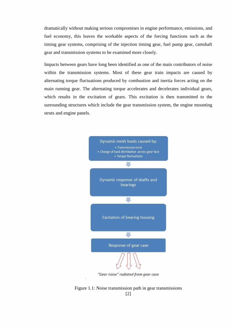
Figure 1.1: Noise transmission path in gear transmissions

[3]
Apart from the engine noise resulting from combustion of fuel, the airborne and structure
borne noise generated from the gear transmission systems make a very significant
contribution to the noise pollution within passenger cars. The gears in mesh cause lateral
and torsional vibrations that make their way through the gear bodies, shafts, bearings and
to the gear housing (Figure 1.1) which transfers this excitation to the surrounding
materials as structural vibration and hence noise. Since each of these components has
respective mass and stiffness, they produce individual frequency responses, amplifying
or attenuating the vibrations on their way to the gear case walls. The noise that is
generated through the flexing of the stiff gear case walls acting as loudspeakers, due to
the structural vibrations is the generated airborne noise. Although both airborne and
structure borne noises are prevalent in vibrating components, the main noise path is the
latter one.
Gear transmissions are an integral part of automotives and other industrial machineries.
In keeping with the current trend towards high mechanical efficiency, the pursuit of
compact and lightweight transmission systems cause an increasing amount of elastic
deformation of the gears. The study and understanding of gear dynamics is
fundamentally important for the monitoring, control and design of better gear
transmission systems. The study of gear dynamics is not a new concept and has been
thoroughly investigated over the last seven decades, starting with Walker in 1938 [4].
Many others including Gregory [5], Harris [6], Ozguven [7], Smith [8] and Welbourn [9]
have produced fundamental publications on various topics in gear dynamics, which
would provide the reader with an insight into the early work in gears.
Although a lot of work has been carried out in the field of gear dynamics, there is still
scope to investigate thoroughly certain areas that were not well developed before. In the
past, the computational limitations were a barrier to certain methods of investigation, and
as a result theoretical and numerical methods were prevalent in trying to understand the
dynamic behaviour of gears [7, 10, 11]. Recent advancements in computational software,
development of numerous finite element analysis (FEA) packages along with faster
computers have aided in some innovative approaches to investigating vibration in gears
[12 – 14].
[4]
As mentioned earlier in this chapter, various factors like torque and geometrical
imperfections have an effect on the vibration and noise generated from a geared system,
and in order to better understand this, one needs to focus on the contact mechanics of the
geared system. In essence, if a gear pair is taken to represent an idealised system with all
the necessary constraints and operating conditions accurately modelled, it would be
possible to analyse the behaviour of the gears under operation.
Most of the research carried out in the last two decades concentrated on the reduction of
noise in gear contact and the hypothesis that transmission error (TE) was the main cause
of most of the noise generated by gear pairs in contact, was developed and established [9,
15 - 17].Transmission error of a gear pair is the difference between the actual position of
the driven gear and the ideal position that the same should have if both driving and
driven gear were undeformed, continuously in contact and in absence of geometrical
imperfections. There have been numerous studies that point out the correlation between
transmission error and noise and several of the key research publications [11, 15, 17, 38,
46, 47] give a very good overview and introduction into the area of transmission error in
gears and most of them establish that the transmission error is one of the main, if not the
cause of gear whine in most gear systems. This should not be confused with the
production of gear whine. Considering that transmission error is a major source of noise,
the actual noise does not come directly from the angular speed variations. As mentioned
earlier, the torsional accelerations cause vibratory bearing reactions that excite the
gearbox casing, which then propagates the noise through the pulsation of the casing
walls.
Many of the theoretical and numerical studies on gear contact have been carried out with
various assumptions with regards to torque, stiffness and geometry of gear systems [18,
19]. The main assumptions in both these cases was the constant torque acting on the
gears and also the exclusion of time varying mesh stiffness in the case of the work
carried out by Kamaya [18]. Although the results of most of these investigations carried
out are widely accepted as quantitatively correct, one wonders if the assumptions could
have made a difference to the outcome. Generally speaking, taking a gear system and
[5]
modelling it without any simplifying assumptions would create a great deal of
complication in solving the equations of motion and extracting a meaningful result.
In recent years, many attempts have been made by numerous authors to set up models
aimed at simulating the dynamic behaviour of gears where the mathematical
formulations range from single-degree-of freedom (SDOF) models to finite element
models (2Dimensional and 3Dimensional), but virtually all gear dynamic models
consider that transmission error (TE) and variations in mesh stiffness are the primary
sources of excitation [5, 6, 7]. A vast number of mathematical models used in gear
dynamics have already been reviewed and classified by Ozguven and Houser [7]. The
sources of mesh excitation and its contribution to system excitation and particularly to
gear noise have also been discussed by Houser [20].
Even though contact mechanics and finite-element analysis (FEA) simulation provide
valuable tools that are used to investigate gear dynamics, there is still a need for more
experimental investigation in order to study the complex non-linear dynamics of geared
systems. Parker [21] has suggested that there is a lack of understanding of the complex
dynamics of geared systems and attributes this to a lack of comprehensive experimental
investigations. The work of Blankenship and Kahraman [22-24] on the single gear pair
system helps in getting a better understanding of the conflicting issues of what is
considered to be a realistic model. Parker [21] has also used FE and contact mechanics
models to study the dynamic response of a spur gear pair across a wide range of
operating speeds and torques.
In the last decade, the general trend has been to reduce TE by optimised profile
modification for specific operating conditions. Sato et al. [25] studied analytically and
experimentally the influence of profile modifications on gear vibration. Tavakoli and
Houser [26] employed an optimisation algorithm based on the modified Complex method
to a particular objective function based on the mean value of harmonics of the
transmission error; different output design torques were considered after the
optimization, but the dynamics was not studied. The static transmission error was
evaluated by means of a cantilever beam model. Several other investigations also focused
on the optimization of profile modifications; for example, Simon [27] and Munro [28]
developed optimization methods based on simplified approaches for teeth deflection. Cai
[6]
and Hayashi [29] firstly employed a nonlinear dynamic model to evaluate the effects of a
static optimisation; the transmission error was evaluated using a simple model based on
elementary formulae and the influence of torque on the optimum profile modification
was also considered. Fonseca et al. [30] optimized the harmonics of the static
transmission error using the same static model of Tavakoli and Houser [26] by means of
a genetic optimization algorithm.
1.2 Scope and objectives
In recent years, there have been considerable developments in direct computer-aided
design (CAD)/computer aided engineering (CAE) data interchange. As a result engineers
can now undertake a wide range of design, analysis, and modelling, on their respective
research areas.
Many research methods use detailed finite element methods to predict TE, but without
the prediction being fully integrated within advanced optimisation procedures, as they
require complete automatic FE solutions. Other research methods involve using finite-
element simulations to get input parameters for simplified analytical dynamic models
(e.g. SDOF mode). Hence considering these factors, there is reasonable scope in
improving the accuracy and robustness of the procedures used and thereby achieving a
higher accuracy of results.
One of the main aims of this project is to develop an FEM procedure which is capable of
modelling gear pairs and gear systems accurately, simulating their respective working
conditions and allowing automated design changes, such as profile modification, within
suitable optimisation algorithms. Currently there are a lot of other simulations on FEM
software such as DuGates, Calyx, and RomaxNVH to name a few, which specialise in
predictive noise and vibration analysis. These are useful in identifying problem sources
in gear designs and rectifying the necessary faults before the design is frozen. The main
difference between the FEM procedure developed in this research work and the above
mentioned softwares is in the innovative approach to solving and reducing the cause of
the main vibration and noise. The main output from the FEM simulation is the
Transmission Error (TE) plots for the respective simulation which give a fairly good
indication to the level of noise that can be generated from the gear pair in question. One
[7]
innovative part of our approach is the fully automated modelling procedure allowing the
study of measures to reduce the TE and hence the vibration and noise generated. Another
innovative aspect is the comparative analysis of the TE evaluated using dynamic
analysis, indicated in the literature as dynamic transmission error (DTE), and the TE
computed using a static analysis, known as static transmission error (STE). The dynamic
analysis in this research is carried out using two approaches: a first one based on
simplified single-DOF dynamic model combined with static FE analysis; a second
approach consisting of a full non-linear finite-element dynamic analysis, which
represents a further original contribution. The work contained in this Thesis is discussed
below in more detail.
1.2.1 Comparison between STE and DTE
One of the main contributions of this work to the field is the comparison between STE
and DTE in gear pairs. The general trend in research at the start was to evaluate the STE
as it was less complex than the DTE and required fewer assumptions such as constant
mesh stiffness, geometrical perfection, and no torque fluctuations [1 – 6]. More recently
there has been an increase of work done on the dynamic aspect of transmission error,
DTE, as it has been reported that the major causes of TE are even more prevalent in this
case [14, 21, 30]. Our research for the first time brings together both avenues of thought
and compares the finding to comment on the efficiency of both methodologies.
1.2.2 Full non-linear dynamic finite-element analyses of gear pair interaction
The determination of the DTE has always been accomplished in the literature using
either entirely analytical approaches, entailing a number of simplifying assumptions, or
using so-called hybrid numerical-analytical methods. In this latter case, a detailed finite-
element model is used in a static analysis to determine the stiffness of the gear pair
interaction as a function of the gear rotation angle. This variable stiffness is then
integrated into a simplified dynamic 1-degree-of-freedom model which is solved using a
numerical procedure.
[8]
Instead, in our research a full non-linear FE dynamic analysis is used to evaluate the
DTE. Various aspects related to this type of analysis are studied in detail and sensitivity
analyses for some of the parameters to be used in the solution procedure and in the
contact algorithm are conducted.
1.2.3 Validation of our FE model with the Hybrid Numerical model
A comparison between the results of full non-linear dynamic analysis and of those
obtained using the hybrid numerical-analytical approaches is also conducted for a wide
range of operating conditions to investigate on the validity of the assumptions made and
on the approximations entailed. Most of the work carried out in the field has got similar
comparisons between their respective numerical models and experimental models [27,
28].
1.2.4 Application of the automated profile modification tool to reduce TE
The main methods implemented to reduce the gear noise and vibration response of the
system are by means of macro-geometry and micro-geometry modifications.
Macro-geometry is defined by gear parameters such as: number of teeth, diameters,
pressure angle, backlash and clearance. Many authors studied the effect of the involute
contact ratio on both spur and helical gear vibrations [18 - 20]. Macro-geometric
modifications involve an important and expensive change of the gear pair as well as the
other members of the gear train; they are feasible only at the first steps of the design
process. High quality surface finishing and strict tolerances can lead to excessive
manufacturing costs; moreover, their effect on vibrations can be disappointingly small.
Micro-geometric modifications consist in an intentional removal of material from the
gear teeth flanks, so that the resulting shape is no longer a perfect involute; such
modifications compensate teeth deflections under load, so that the resulting transmission
error is minimized for a specific torque. In this study, the micro-geometry modifications
will be the focus of the analysis and are investigated with a view to developing fully
automated design optimisation algorithms.
[9]
1.3 Outline of Thesis
This thesis is comprised of a total of nine chapters. The first chapter is a general
introduction into the subject of noise within the mechanical sense, and the discussion of
subsequent research work carried out in the field of gear noise and vibration. The link
between the overall noise in an automotive setting is related to the gear transmission and
employed to summarise the research’s aims and objectives.
Chapter 2 provides a review of the fundamentals of gears starting with a brief history and
the ideology behind gears. The chapter also proceeds to discuss the common types of
gears used in the industry and provides reasons for choosing spur gears for our research.
Finally, introductions into the essential aspects of spur gear design are examined in order
to give the reader an insight into the research work.
In Chapter 3, the general field of gear noise and vibration is described and the literature
review of this field is provided. This chapter affords an important function to this
research by collating all the pertinent work carried out within the field of gear noise. This
chapter also bridges the relationship between the research carried out and its effect on the
broader picture of engines. Technical publications of relevant works are summarised and
conclusions draw on existing work relating to this research. The topic of transmission
error is introduced and discussed with respect to the sources and types most commonly
researched in the last few decades.
Chapter 4 considers the details of spur gear design with respect to performance
characteristics. The main aspects of stress formulae, design limits, strength and durability
calculations are examined along detailed work involved in designing a spur gear. Finally
calculations are carried out to enable the gear designer to choose the right variables in
terms of module, tooth thickness, tooth size and base radius, for the relevant application.
In this project however, the calculations are intended to give the reader a general
understanding of the basic information needed to design a gear, and then leading into the
calculations used to derive the spur gear involute profile for the PYTHON scripts.
[10]
In Chapter 5, a procedure to model the geometry of a pair of spur gears in the finite-
element code ABAQUS and to input material properties, loading and boundary
conditions for static and dynamic analyses is presented. The case is considered in which
the angular velocity is prescribed for the driving gear and the torque is assigned for the
driven gear. The procedure has been implemented into a Python script so that the user
only has to input the macro-geometrical parameters of the gear, as well as the prescribed
angular velocity and torque, and run the analysis with the click of a button.
Chapter 6 presents the development of the numerical model of the two pair gear model
system using equations of motion, where the formulation for the transmission error is
also derived. The model in this chapter has two degrees of freedom gear model and is a
modified version of models widely used in literature. The basic characteristic of our
model is that it is a model with tooth compliance and has been modified to suit our
methodology and will be explained further in this chapter. The results of the hybrid
numerical/analytical model are also discussed in this chapter in relation to initial and
boundary conditions.
Chapter 7 presents the main contributions from this thesis which are organised within
this chapter along with some of the significant results. The methodology used to conduct
a static non-linear finite-element analysis is described and results are presented for a
number of spur gear pairs and operating conditions. In Section 7.3 the STE obtained
using a non-linear static analysis is compared with the DTE obtained using the single-
DOF hybrid numerical/analytical method for a number of gear geometries and of
operating conditions. The results of this comparison are quite interesting and will be
carefully discussed. In Section 7.4 the results of the hybrid numerical/analytical
simulations are compared with those provided by a full non-linear dynamic analysis and
it is shown that great attention has to be paid to the parameters used in contact algorithm
used in the FE simulations for this comparison to be correct and meaningful. In the same
chapter further sensitivity analysis of the FE simulation to mesh refinement, convergence
tolerance and time increment size are presented for completeness.
[11]
In Chapter 8, the procedures for the optimisation of profile modifications are developed
to reduce the rotational vibrations of a spur gear pair. Further research into the effect of
tooth profile modifications on the transmission error of gear pairs is carried out. A
detailed parametric study, involving development of an optimisation algorithm to design
the tooth modifications, is performed to quantify the changes in the transmission error as
a function of tooth profile modification parameters as compared to an unmodified gear
pair baseline.
Finally Chapter 9 summarises the general conclusions of this thesis and recollects the
main contributions to the area of gear noise analysis, gear transmission error prediction
and transmission error reduction through tooth profile modification along with some
recommendations for future work.
[12]
2. FUNDAMENTALS OF GEAR DESIGN
2.1 Introduction
Gears have been widely used in most types of machineries since the start of the industrial
revolution. Along with bolts, nuts and screws, they are a common element in machines
and will be needed frequently by machine designers to realise their designs in almost all
fields of mechanical applications. Ever since the first gear was conceived over 3000
years ago, they have become an integral component in all manner of tools and
machineries since then.
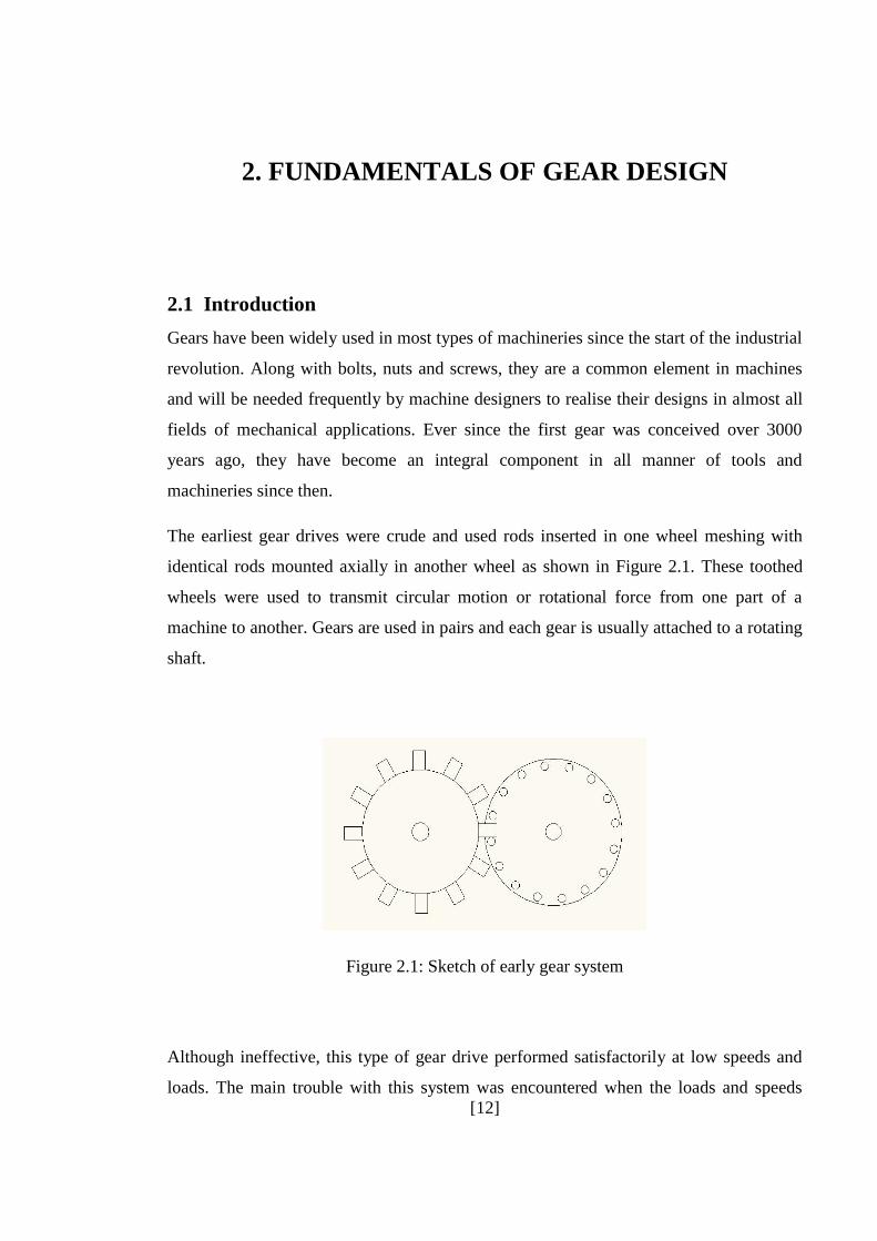
The earliest gear drives were crude and used rods inserted in one wheel meshing with
identical rods mounted axially in another wheel as shown in Figure 2.1. These toothed
wheels were used to transmit circular motion or rotational force from one part of a
machine to another. Gears are used in pairs and each gear is usually attached to a rotating
shaft.
Figure 2.1: Sketch of early gear system
Although ineffective, this type of gear drive performed satisfactorily at low speeds and
loads. The main trouble with this system was encountered when the loads and speeds

[13]
were raised. The contact between the rods were in effect a point contact, giving rise to
very high stresses which the materials could not withstand and the use of any lubrication
was obsolete due to the contact area, hence high wear was a common occurrence.
Although not so obvious at the time, the understanding of the speed ratio of the gear
system was critical. Due to the crude design of the system, the speed ratio was not
constant. As a result, when one gear ran at constant speed, there was regular acceleration
and deceleration of each teeth of the other gear. The loads generated by the acceleration
influenced the steady drive loads to cause vibration and ultimately failure of the gear
system.
Since the 19th
century the gear drives designed have mainly been concerned with keeping
contact stresses below material limits and improving the smoothness of the drive by
keeping velocity ratios as constant as possible. The major rewards of keeping the velocity
ratio constant is the reduction of dynamic effects which will give rise to stress increases,
vibration and noise.
Gear design is a highly complicated skill, and the constant pressure to build cheaper,
quieter running, lighter and more powerful machinery has given rise to steady and
advantageous changes in gear designs over the past few decades.
2.2 Types of gears
There are many different types of gears currently being designed, manufactured and used
in the world today. There is an abundance of literature on the types of gears, their main
characteristics, materials used and suitability of applications in the following books [8,
39, 45, 74, 75, 78]. The main types are spur gears, helical gears, bevel gears and worm
gears.
2.2.1 Spur gears
Spur gears have teeth parallel to the axis of rotation (Figure 2.2) and are used to transmit
power and rotation from one shaft to another. The spur gear is the simplest type of gear
form and all other types of gears are based on the spur gear shape. Most manufacturers
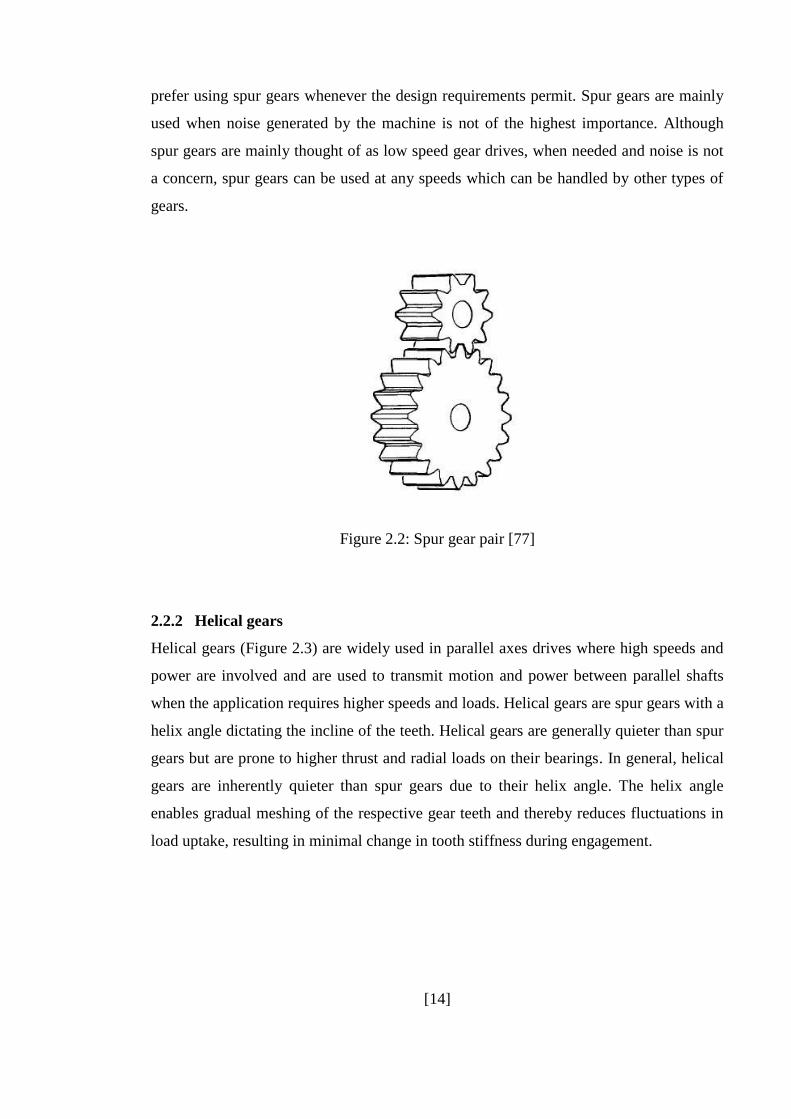
[14]
prefer using spur gears whenever the design requirements permit. Spur gears are mainly
used when noise generated by the machine is not of the highest importance. Although
spur gears are mainly thought of as low speed gear drives, when needed and noise is not
a concern, spur gears can be used at any speeds which can be handled by other types of
gears.
Figure 2.2: Spur gear pair [77]
2.2.2 Helical gears
Helical gears (Figure 2.3) are widely used in parallel axes drives where high speeds and
power are involved and are used to transmit motion and power between parallel shafts
when the application requires higher speeds and loads. Helical gears are spur gears with a
helix angle dictating the incline of the teeth. Helical gears are generally quieter than spur
gears but are prone to higher thrust and radial loads on their bearings. In general, helical
gears are inherently quieter than spur gears due to their helix angle. The helix angle
enables gradual meshing of the respective gear teeth and thereby reduces fluctuations in
load uptake, resulting in minimal change in tooth stiffness during engagement.

[15]
Figure 2.3: Helical gear pair [77]
2.2.3 Bevel gears
Bevel gears are conical in shape and the teeth cut from them are tapered in both tooth
thickness and height (Figure 2.4). Bevel gears are mostly used to transmit motion
between intersecting shafts where the shaft angle is usually 90°. The motion of the bevel
gears produce radial and thrust loads on their bearings. The most commonly used are the
straight tooth bevel gears. A modification to the straight tooth bevel gear gives the spiral
tooth bevel gear (Figure 2.5) which has teeth that are both curved along the tooth's length
and set at an angle. Spiral tooth bevel gears have the same advantages and disadvantages
in relation to the straight tooth bevel gears as helical gears do to spur gears. In general
bevel gears are designed to operate with 98% efficiency or better [74].
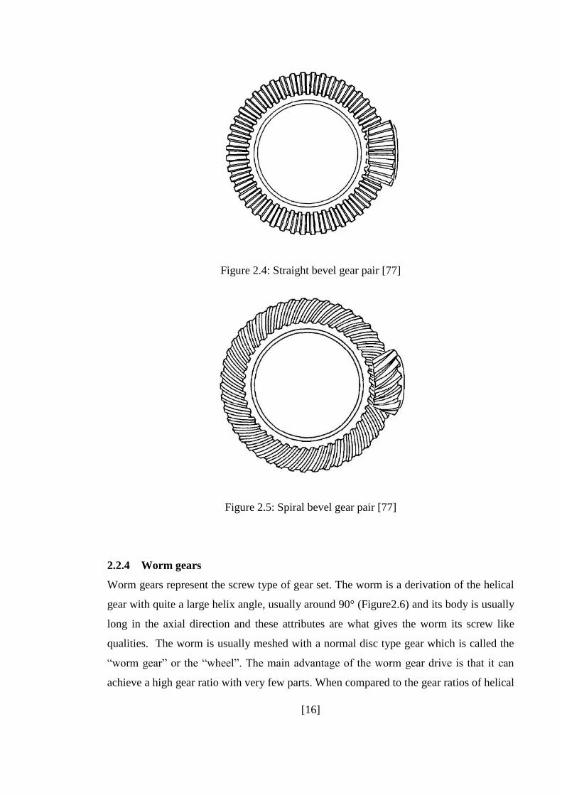
[16]
Figure 2.4: Straight bevel gear pair [77]
Figure 2.5: Spiral bevel gear pair [77]
2.2.4 Worm gears
Worm gears represent the screw type of gear set. The worm is a derivation of the helical
gear with quite a large helix angle, usually around 90° (Figure2.6) and its body is usually
long in the axial direction and these attributes are what gives the worm its screw like
qualities. The worm is usually meshed with a normal disc type gear which is called the
“worm gear” or the “wheel”. The main advantage of the worm gear drive is that it can
achieve a high gear ratio with very few parts. When compared to the gear ratios of helical
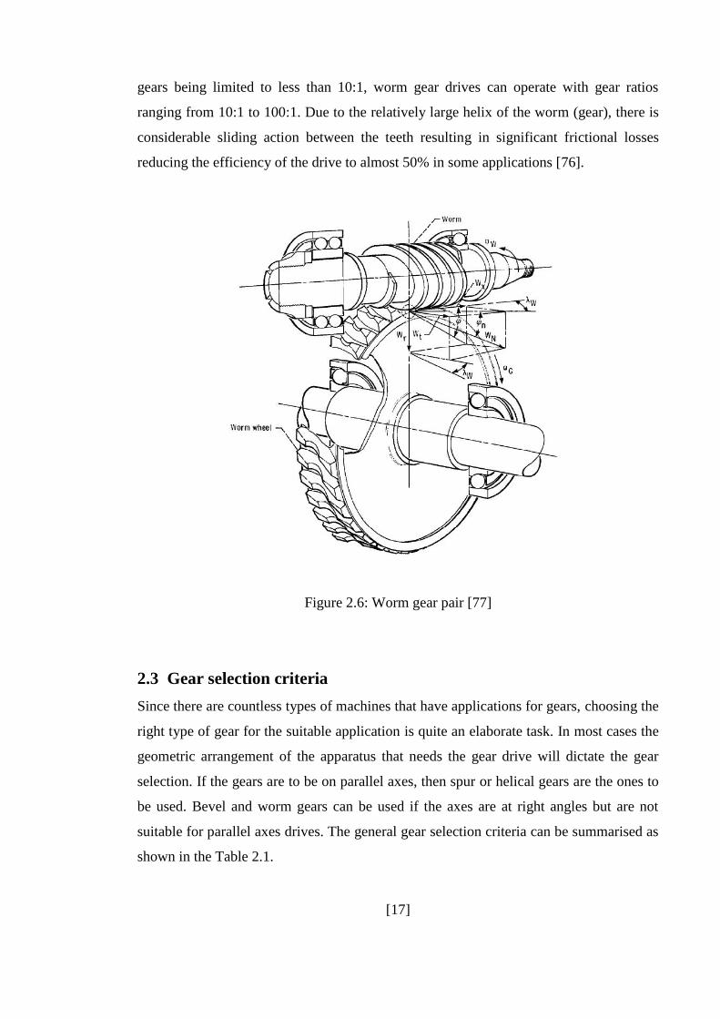
[17]
gears being limited to less than 10:1, worm gear drives can operate with gear ratios
ranging from 10:1 to 100:1. Due to the relatively large helix of the worm (gear), there is
considerable sliding action between the teeth resulting in significant frictional losses
reducing the efficiency of the drive to almost 50% in some applications [76].
Figure 2.6: Worm gear pair [77]
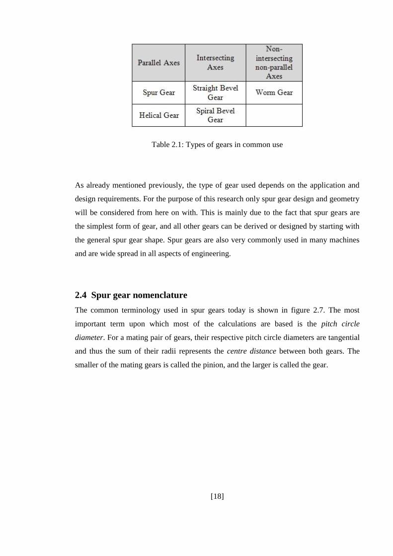
2.3 Gear selection criteria
Since there are countless types of machines that have applications for gears, choosing the
right type of gear for the suitable application is quite an elaborate task. In most cases the
geometric arrangement of the apparatus that needs the gear drive will dictate the gear
selection. If the gears are to be on parallel axes, then spur or helical gears are the ones to
be used. Bevel and worm gears can be used if the axes are at right angles but are not
suitable for parallel axes drives. The general gear selection criteria can be summarised as
shown in the Table 2.1.
[18]
Table 2.1: Types of gears in common use
As already mentioned previously, the type of gear used depends on the application and
design requirements. For the purpose of this research only spur gear design and geometry
will be considered from here on with. This is mainly due to the fact that spur gears are
the simplest form of gear, and all other gears can be derived or designed by starting with
the general spur gear shape. Spur gears are also very commonly used in many machines
and are wide spread in all aspects of engineering.
2.4 Spur gear nomenclature
The common terminology used in spur gears today is shown in figure 2.7. The most
important term upon which most of the calculations are based is the pitch circle
diameter. For a mating pair of gears, their respective pitch circle diameters are tangential
and thus the sum of their radii represents the centre distance between both gears. The
smaller of the mating gears is called the pinion, and the larger is called the gear.
[19]
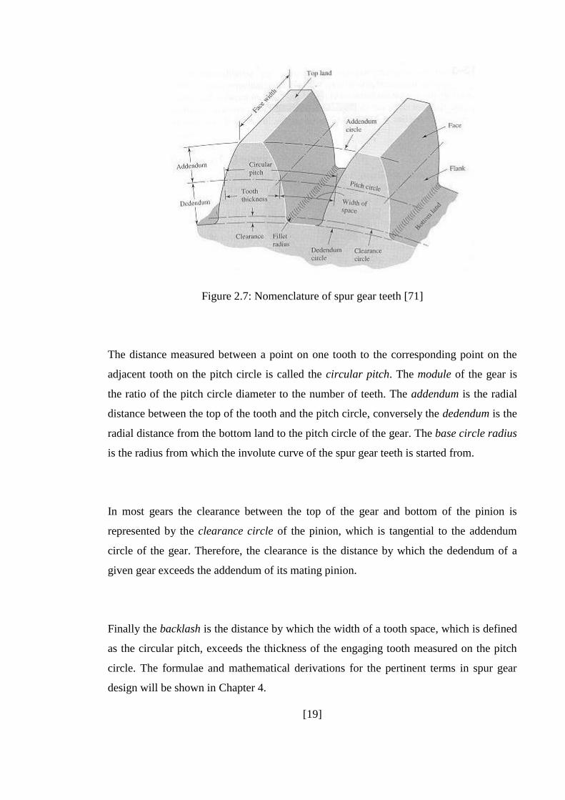
Figure 2.7: Nomenclature of spur gear teeth [71]
The distance measured between a point on one tooth to the corresponding point on the
adjacent tooth on the pitch circle is called the circular pitch. The module of the gear is
the ratio of the pitch circle diameter to the number of teeth. The addendum is the radial
distance between the top of the tooth and the pitch circle, conversely the dedendum is the
radial distance from the bottom land to the pitch circle of the gear. The base circle radius
is the radius from which the involute curve of the spur gear teeth is started from.
In most gears the clearance between the top of the gear and bottom of the pinion is
represented by the clearance circle of the pinion, which is tangential to the addendum
circle of the gear. Therefore, the clearance is the distance by which the dedendum of a
given gear exceeds the addendum of its mating pinion.
Finally the backlash is the distance by which the width of a tooth space, which is defined
as the circular pitch, exceeds the thickness of the engaging tooth measured on the pitch
circle. The formulae and mathematical derivations for the pertinent terms in spur gear
design will be shown in Chapter 4.
[20]
2.5 Velocity ratio
As mentioned in the introduction of this chapter, the speed or velocity ratio of a gear
drive is important and is essential in determining the geometric make up of the gear
drive.
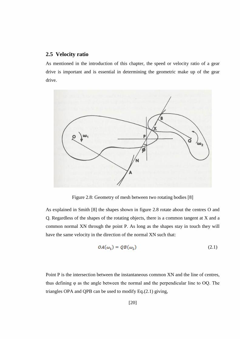
Figure 2.8: Geometry of mesh between two rotating bodies [8]
As explained in Smith [8] the shapes shown in figure 2.8 rotate about the centres O and
Q. Regardless of the shapes of the rotating objects, there is a common tangent at X and a
common normal XN through the point P. As long as the shapes stay in touch they will
have the same velocity in the direction of the normal XN such that:
(2.1)
Point P is the intersection between the instantaneous common XN and the line of centres,
thus defining φ as the angle between the normal and the perpendicular line to OQ. The
triangles OPA and QPB can be used to modify Eq.(2.1) giving,
[21]
(2.2)
(2.3)
Therefore the only requirement for a constant velocity ratio is that the ratio of centre
distances remains constant, ensuring that the common normal passes through the pitch
point, P.
2.6 Conjugate action
The mating teeth of gears acting against each other are like cams and produce rotary
motion as a result. Considering the gear teeth to be perfectly formed, smooth and rigid,
although highly unrealistic, helps demonstrate the principle of conjugate action.
When gear teeth have been so designed to produce a constant angular velocity ratio
between the gear pair on meshing, they are said to have conjugate action. This action can
be further analysed using the figure 2.9 shown below.
[22]
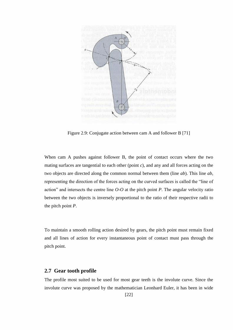
Figure 2.9: Conjugate action between cam A and follower B [71]
When cam A pushes against follower B, the point of contact occurs where the two
mating surfaces are tangential to each other (point c), and any and all forces acting on the
two objects are directed along the common normal between them (line ab). This line ab,
representing the direction of the forces acting on the curved surfaces is called the “line of
action” and intersects the centre line O-O at the pitch point P. The angular velocity ratio
between the two objects is inversely proportional to the ratio of their respective radii to
the pitch point P.
To maintain a smooth rolling action desired by gears, the pitch point must remain fixed
and all lines of action for every instantaneous point of contact must pass through the
pitch point.
2.7 Gear tooth profile
The profile most suited to be used for most gear teeth is the involute curve. Since the
involute curve was proposed by the mathematician Leonhard Euler, it has been in wide

[23]
use in the mechanical industry. This is mainly due to the meshing of the involute profile
gear teeth not being easily disturbed by small errors in centre distance of the gear pairs
and the ease of manufacturing of the involute gear tooth. If a point on the end of a string
being unwound from a cylinder of fixed radius could be traced, the curve produced by
this trace would be that of an involute (Figure 2.10).
Figure 2.10: Generation of involute curve [77]
The more modern Wildhaber-Novikov gears use another type of profile based on the
cycloid form. Almost all gear forms based on the cycloid are very sensitive to centre
distance, which can be a big disadvantage. Generally speaking, higher levels of noise and
vibration are generated in a structure when the size of a force varies with time or the
point of application or direction of force varies. This is not a problem with the involute
profile which allows both the normal and the force to keep acting in the same direction,
unlike that of cycloid gears where the normal can be designed to pass through the pitch
point, but allowing the direction of force to vary, hence generating more noise.
Over time, the involute curve has remained the favoured gear profile, primarily due to the
ease of manufacture and its adaptability to centre distance. In terms of vibration, it is the
only type of profile that gives constant force, direction and position for applications
where low vibration is essential.
[24]
2.8 Standardisation of gears
Gears of varying sizes and geometry are used in all manner of applications in the
industry, and the method of identifying and logically specifying common types of gears
for applications are based on their exact pitch distances. Thus the module m, has been
identified and defined as the ratio between the centre distance and number of teeth on the
pitch circle diameter. This is the definition in the metric system and is measured in mm.
(2.4)
In most gears, the pressure angle has now been standardised to but angles between
and are occasionally used depending on the application.
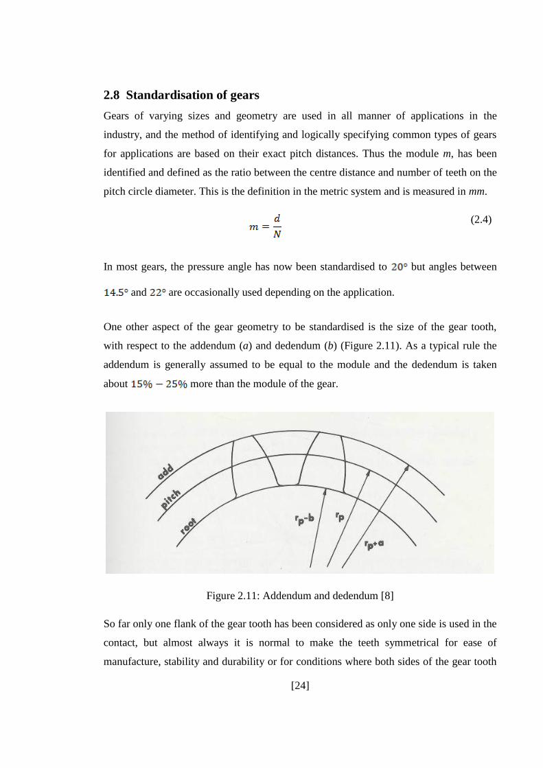
One other aspect of the gear geometry to be standardised is the size of the gear tooth,
with respect to the addendum (a) and dedendum (b) (Figure 2.11). As a typical rule the
addendum is generally assumed to be equal to the module and the dedendum is taken
about more than the module of the gear.
Figure 2.11: Addendum and dedendum [8]
So far only one flank of the gear tooth has been considered as only one side is used in the
contact, but almost always it is normal to make the teeth symmetrical for ease of
manufacture, stability and durability or for conditions where both sides of the gear tooth

[25]
flanks are used, such as in an idler gear in vehicle transmission. Taking this into account,
a clearance, usually called backlash, should be included between the non-working flanks
of gear pair, or else forces and wear rates are high. The backlash coefficient in gears is
usually not less than although precision drives and servos may require even
lower values.
2.9 Contact ratio of gears
When two gear teeth mesh, the meshing zone is usually limited between the intersecting
radii of addendum of the respective gears, as shown in Figure 2.12. From the figure it can
be seen that the initial tooth contact occurs at a and final tooth contact occurs at b. If the
respective tooth profiles are drawn through points a and b, they will each intersect the
pitch circle at points A and B respectively. The radial distance AP is called the arc of
approach qa, and the radial distance PB is called the arc of recess qr; the sum of these
being the arc of action qt.
(2.5)
Figure 2.12: Contact ratio [71]
[26]
When the circular pitch p of a mating gear pair is equal to the arc of action qt, there is
always only one pair of teeth in contact, one gear tooth and one pinion tooth in contact
and their clearance occupies the space between the arc AB.
(2.6)
In this case , and, as the contact is ending at b, another tooth simultaneously starts
contact at a. In other situations, when the arc of action is greater than the circular pitch,
more than one tooth of the gear is always in contact with more than one tooth in the
pinion, meaning that as one tooth is ending contact at b, another tooth is already been in
contact for a small period of time starting at a. For a short period of time there will be
two teeth in contact, one near A and the other near B. As the gear pair rotates through
their meshing cycle, the tooth near B will cease to be in contact and only a single pair of
contacting teeth will remain, and this process repeats itself over the period of operation.
The contact ratio mc is given by
(2.7)
and provides the average number of teeth pairs in contact
Most gears are generally designed with a contact ratio of more than 1.20, as the contact
ratio is generally reduced due to errors in mounting and assembly of the gear pairs. Gear
pairs operating with low contact ratios are susceptible to interference and damage as a
result of impacts between teeth and thereby leading to an increased level of noise and
vibration.
Gears are generally designed with contact ratios of 1.2 to 1.6. A contact ratio of 1.6, for
example, means that 40 percent of the time one pair of teeth will be in contact and 60
percent of the time two pairs of teeth will be in contact. A contact ratio of 1.2 means that
80 percent of the time one pair of teeth will be in contact and 20 percent of the time two
pairs of teeth will be in contact. Gears with contact ratios greater than 2 are referred to as
“high-contact-ratio gears.” For these gears there are never less than two pairs of teeth in
contact. A contact ratio of 2.2 means that 80 percent of the time two pairs of teeth will be
in contact and 20 percent of the time three pairs of teeth will be in contact. High-contact-

[27]
ratio gears are generally used in select applications where long life is required. Analyses
should be performed when using high-contact-ratio gearing because higher bending
stresses may occur in the tooth addendum region. Also, higher sliding in the tooth contact
can contribute to distress of the tooth surfaces. In addition, higher dynamic loading may
occur with high-contact ratio gearing
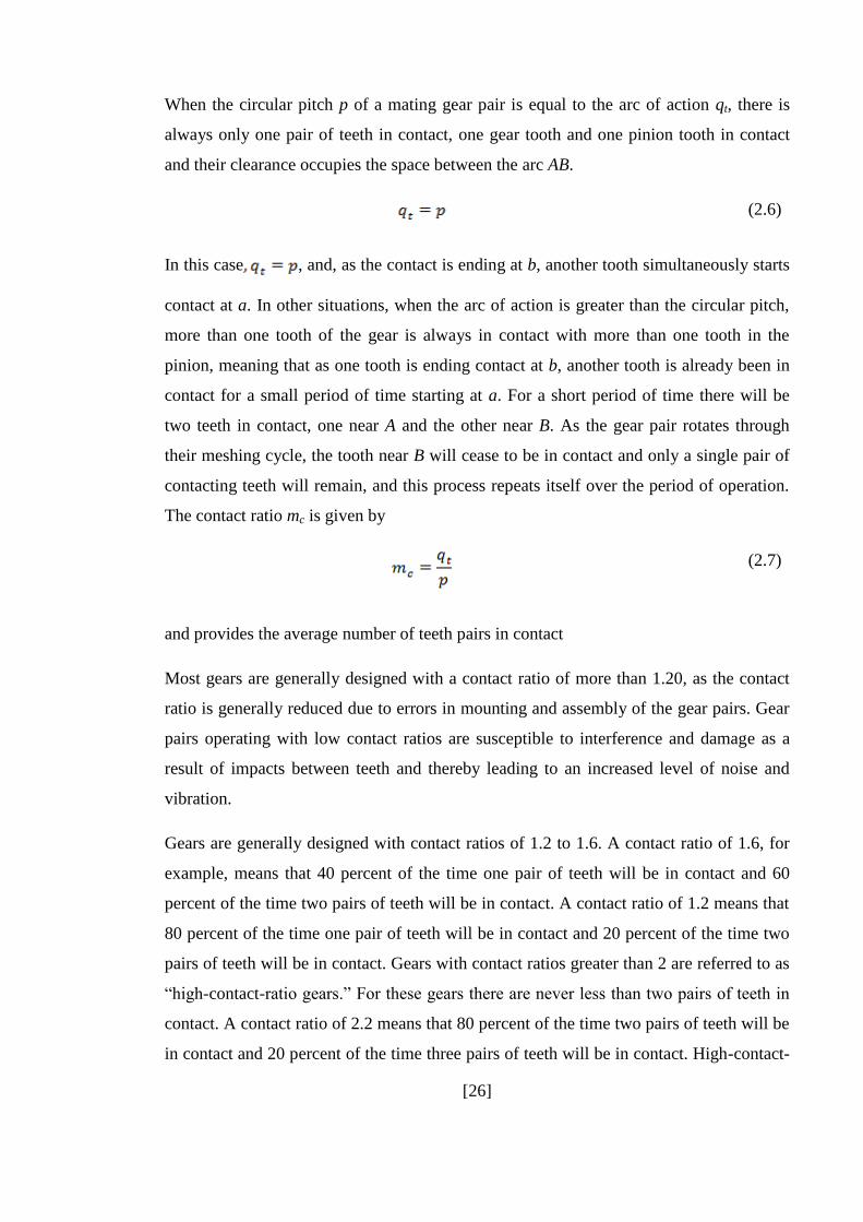
2.10 Interference in gears
When gear pairs are meshed and contact occurs outside the zone of action, essentially in
portions of the gear tooth profiles that are not conjugate, interference is said to occur. In
figure 2.13, a meshing gear pair with equal number of teeth is shown with the driver
turning clockwise. The initial and final contact points as before have been designated as
A and B respectively, on the pressure line. The line of tangency between the respective
base circles indicates the line of action between the gear pairs, and observing that the
points of tangency C and D are located inside points of A and B, it can be said with
certainty that there will be interference in contact.
[28]
Figure 2.13: Interference between gear teeth [71]
When the gears mesh, at the start of contact, the tip of the driven gear tooth makes
contact with the flank of the driving gear tooth at point A, occurring before the involute
portion of the gear tooth comes into range. The effect of this is the involute tip of the
driven gear digging into the non-involute flank of the driving gear. This can usually be
avoided by most tooth generation processes by undercutting the tooth profile of the gears.
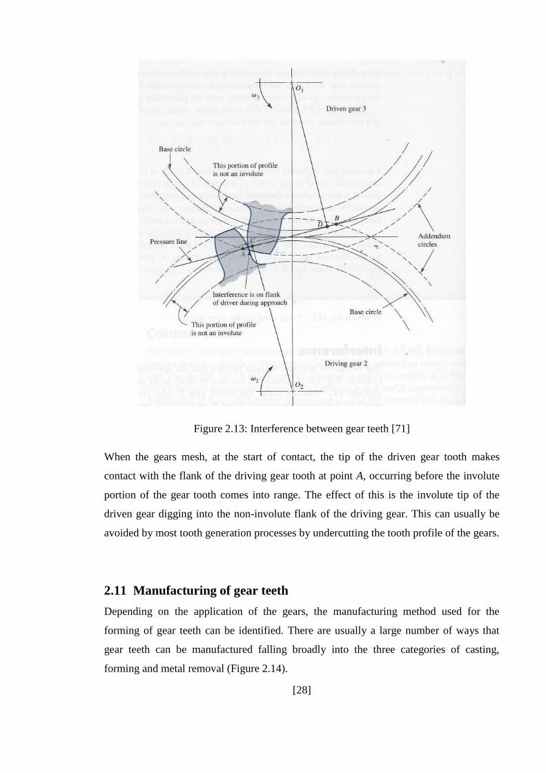
2.11 Manufacturing of gear teeth
Depending on the application of the gears, the manufacturing method used for the
forming of gear teeth can be identified. There are usually a large number of ways that
gear teeth can be manufactured falling broadly into the three categories of casting,
forming and metal removal (Figure 2.14).
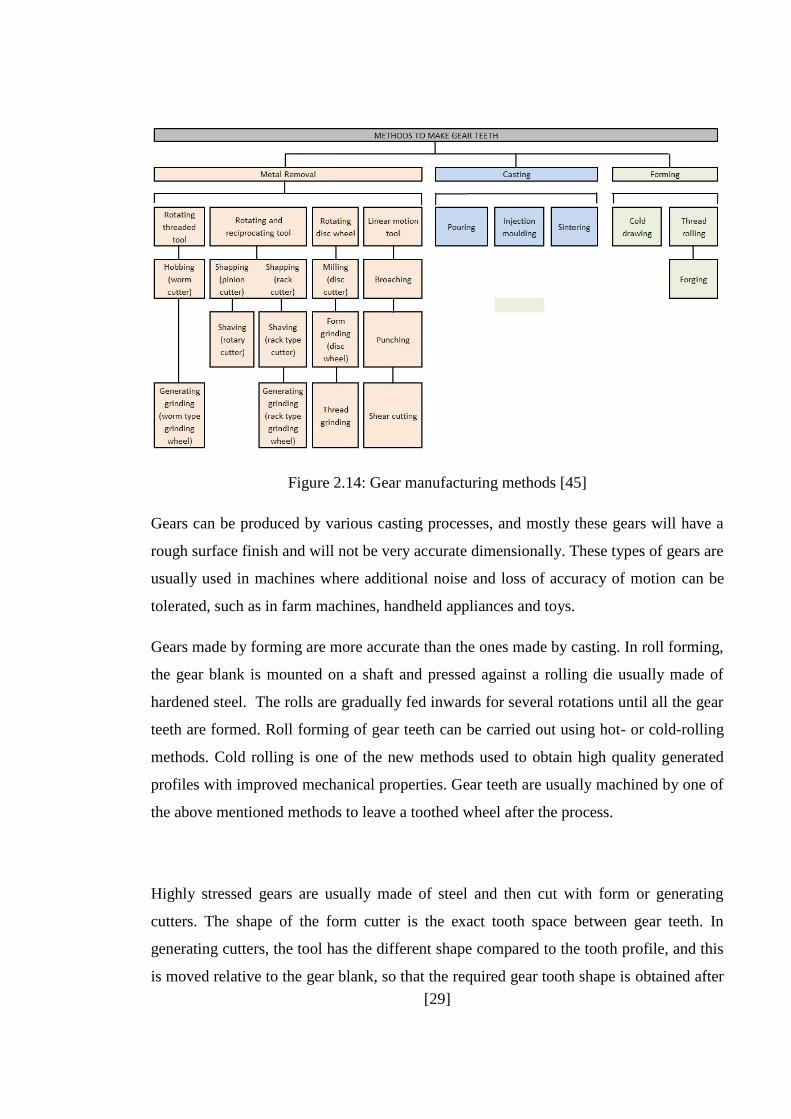
[29]
Figure 2.14: Gear manufacturing methods [45]
Gears can be produced by various casting processes, and mostly these gears will have a
rough surface finish and will not be very accurate dimensionally. These types of gears are
usually used in machines where additional noise and loss of accuracy of motion can be
tolerated, such as in farm machines, handheld appliances and toys.
Gears made by forming are more accurate than the ones made by casting. In roll forming,
the gear blank is mounted on a shaft and pressed against a rolling die usually made of
hardened steel. The rolls are gradually fed inwards for several rotations until all the gear
teeth are formed. Roll forming of gear teeth can be carried out using hot- or cold-rolling
methods. Cold rolling is one of the new methods used to obtain high quality generated
profiles with improved mechanical properties. Gear teeth are usually machined by one of
the above mentioned methods to leave a toothed wheel after the process.
Highly stressed gears are usually made of steel and then cut with form or generating
cutters. The shape of the form cutter is the exact tooth space between gear teeth. In
generating cutters, the tool has the different shape compared to the tooth profile, and this
is moved relative to the gear blank, so that the required gear tooth shape is obtained after
[30]
a full revolution of the gear blank. Generating gears from gear blanks is one of the most
accurate ways of obtaining high-precision gears; this is mainly due to the stiffness
between the gear blank and the cutter during the generating procedure.
2.11.1 Milling
Some gear teeth are cut with a form miller cutting tool shaped to fit the exact tooth space
between gear teeth. Using this method, requires different tools for different sets of gears,
and is hence expensive compared to other forms of cutters. The cutting tool is usually a
toothed disc with the “gear tooth space” contour ground into the sides of the teeth.
2.11.2 Shaping
This is the most common type of generating cutter where the teeth is generated either
with a pinion or rack cutter. The pinion cutter is used to cut along the vertical axis by
cutting the gear blank to the required depth. Each tooth of the pinion cutter is a cutting
tool, so the gear geometry is complete after a complete rotation of the blank.
2.11.3 Hobbing
Almost all types of gears including spur, helical and worm gears can be produced by the
hobbing technique, with the only exceptions being internal gears. The hobbing machine
is essentially a specialised version of a milling tool, where a cutting tool (the hob),
progressively makes a series of cuts into the gear blank to generate the required teeth
shape. The hobbing machine works with two non-parallel spindles, one carrying the gear
blank and the other mounted with the hob. In the hobbing process, the cutting tool is
usually cylindrical with helical cutting teeth that have grooves running the length of the
hob in order to aid in cutting and chip removal. The hob is thus used to create spur and
helical gears by being fed hob across the face width of the gear blank and thus cutting the
required teeth profile. In the case of the worm gear, the hob is generally passed
tangentially past the blank or radially into the blank.
[31]
The important factor, that decides which type of manufacturing method is chosen in the
manufacture of the gear, depends on the intended application of the gear and the
resources available for the application. There is in effect a trade-off between cost and
accuracy in the manufacturing methods discussed above. The cheaper options of casting
and forming will provide relatively good gears that can perform the desired tasks but
always with a slight loss of accuracy, whereas, the more accurate generating processes
will provide high-precision gears at a cost.
2.12 Spur gears
The external spur gear (figure 2.2) is the most common type of gear. Since the teeth are
straight and parallel to the shaft axis, it is also the simplest type of gear. In most
applications the pinion is the driving element and the gear is the driven element. Most
spur gear tooth profiles are cut to conform to an involute curve in order to ensure
conjugate action. Well designed spur gears are also manufactured using castings of a
high standard.
The line of action, or pressure line (fig. 2.15), is the line that is tangent to both base
circles. All points of contact between the two teeth will lie along this line. The pressure
angle φ is defined as the acute angle between the line of action and a line perpendicular
to the line of centers.
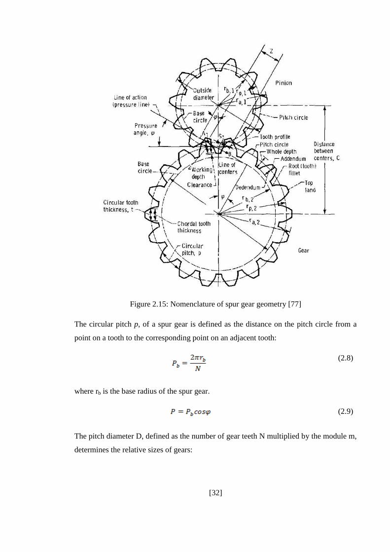
[32]
Figure 2.15: Nomenclature of spur gear geometry [77]
The circular pitch p, of a spur gear is defined as the distance on the pitch circle from a
point on a tooth to the corresponding point on an adjacent tooth:
(2.8)
where rb is the base radius of the spur gear.
(2.9)
The pitch diameter D, defined as the number of gear teeth N multiplied by the module m,
determines the relative sizes of gears:
[33]
(2.10)
(2.11)
The circular pitch, p is defined as the multiple of the module and π. The distance between
the centre of the gears is shown in figure 2.16, and is defined as
(2.12)
The space between the teeth must be larger than the mating tooth thickness in order to
prevent jamming of the gears. The difference between tooth thickness and tooth space as
measured along the pitch circle is called backlash. Backlash can be created by cutting the
gear teeth slightly thinner than the space between teeth, or by setting the center distance
slightly greater between the two gears. In the second case the operating pressure angle of
the gear pair is increased accordingly. The backlash for a gear pair must be sufficient to
permit free action under the most severe combination of manufacturing tolerances and
operating temperature variations. Backlash should be small in positioning control
systems, but it should be quite generous for single-direction power gearing (table 2). If
the center distance between mating external gears is increased by , the resulting
increase in backlash is
(2.13)
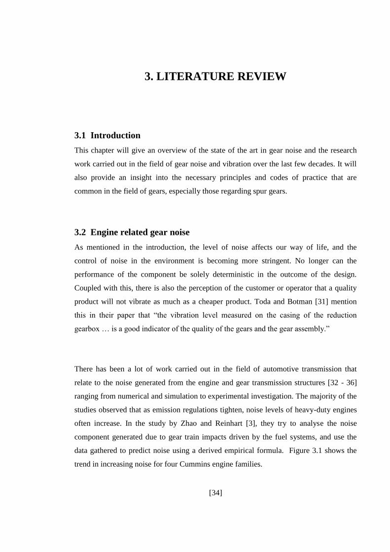
[34]
3. LITERATURE REVIEW
3.1 Introduction
This chapter will give an overview of the state of the art in gear noise and the research
work carried out in the field of gear noise and vibration over the last few decades. It will
also provide an insight into the necessary principles and codes of practice that are
common in the field of gears, especially those regarding spur gears.
3.2 Engine related gear noise
As mentioned in the introduction, the level of noise affects our way of life, and the
control of noise in the environment is becoming more stringent. No longer can the
performance of the component be solely deterministic in the outcome of the design.
Coupled with this, there is also the perception of the customer or operator that a quality
product will not vibrate as much as a cheaper product. Toda and Botman [31] mention
this in their paper that “the vibration level measured on the casing of the reduction
gearbox … is a good indicator of the quality of the gears and the gear assembly.”
There has been a lot of work carried out in the field of automotive transmission that
relate to the noise generated from the engine and gear transmission structures [32 - 36]
ranging from numerical and simulation to experimental investigation. The majority of the
studies observed that as emission regulations tighten, noise levels of heavy-duty engines
often increase. In the study by Zhao and Reinhart [3], they try to analyse the noise
component generated due to gear train impacts driven by the fuel systems, and use the
data gathered to predict noise using a derived empirical formula. Figure 3.1 shows the
trend in increasing noise for four Cummins engine families.
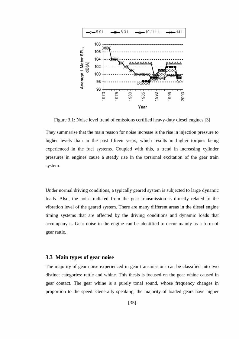
[35]
Figure 3.1: Noise level trend of emissions certified heavy-duty diesel engines [3]
They summarise that the main reason for noise increase is the rise in injection pressure to
higher levels than in the past fifteen years, which results in higher torques being
experienced in the fuel systems. Coupled with this, a trend in increasing cylinder
pressures in engines cause a steady rise in the torsional excitation of the gear train
system.
Under normal driving conditions, a typically geared system is subjected to large dynamic
loads. Also, the noise radiated from the gear transmission is directly related to the
vibration level of the geared system. There are many different areas in the diesel engine
timing systems that are affected by the driving conditions and dynamic loads that
accompany it. Gear noise in the engine can be identified to occur mainly as a form of
gear rattle.
3.3 Main types of gear noise
The majority of gear noise experienced in gear transmissions can be classified into two
distinct categories: rattle and whine. This thesis is focused on the gear whine caused in
gear contact. The gear whine is a purely tonal sound, whose frequency changes in
proportion to the speed. Generally speaking, the majority of loaded gears have higher
[36]
levels of sound generated when compared to unloaded gears, but both have the same
sound characteristics.
Comparatively, gear rattle is generally associated with lightly loaded or unloaded gears;
with the exception of certain systems which have been known to rattle at more
substantial loads.
3.3.1 Gear rattle in gear transmissions
The gear rattling is often caused by large gear backlash. Unlike gear transmission for
spark ignition (SI) engines, highly alternating torque fluctuations act on the gear train of
diesel engines. These alternating torque fluctuations are produced by combustion and
inertia forces acting on the main running gear as well as the inertia, spring and hydraulic
forces in the valve gear and injection pump. The alternate torques accelerates and
decelerates individual gears, which results in motion through clearances in the gear train
and this excitation of gears.
The gear rattle can be separated into two actions: separation and impact. Referring to the
case study by Y Mura et al. [36], Mura observed that the crankshaft and camshaft gear
teeth separate when the peak of the phase difference caused by meshing error between
both gears coincide with the ridge of the engine revolution fluctuation and also then
collide when the relative velocity is too large. The impact of the collision is further
increased if the degree of separation is large and the collision occurs at the peak of the
injection pump drive torque.
H. Lahey et al [37] investigated the gear train related noise as a direct result of high
pressure injection systems. They worked on a methodology that has a finite element
analysis coupled with a multi body system analysis to analyse the gear dynamics within
the system and aid in optimizing the resulting noise. Their study correlates with the work
published my Y. Miura [36] and states that the main gear train noise excitation is caused
by tooth impact due to torque fluctuations. These torque fluctuations are caused by

[37]
intermitting combustion, irregular torque demand of the auxiliaries (e.g. the injection
system) and torsional vibrations of the crankshaft.
It can be summarised that the gear rattle phenomenon centres on the separation and
impact of gear teeth. The magnitudes of the impacts are clearly proportional to the
relative velocities of the gear bodies, and also seem to depend on the amount of backlash
between gears. Although the backlash is not the direct cause of gear rattle, it has been
shown in the work carried out by Huang and Abram [2] that minimising the amount of
backlash between gears prevents large tooth velocities and reduces the level of noise
generated as a result of gear impacts. This is significant in the low idle conditions where
the gears are lightly loaded and optimising the backlash yielded a noise reduction of 2
dB. There has been a significant amount of work done on this phenomenon of gear rattle,
but this fascinating non-linear dynamics problem is not the main focus of this thesis, so
from this point on all “gear noise” will be making reference to the “gear whine” aspect of
noise.
3.3.2 Gear whine in gear dynamics
The gear whine caused when two gears mesh is a slightly more complex process to
understand. It is mainly caused by one or a combination of the following factors:
transmission error, torsional mesh stiffness, axial forces, frictional forces, lubricant
entrainment and air entrapment as suggested by few researchers including Munro and
Houser [38]. The work done by the above is a very good starting point for any research
work in the area of gear noise and as such provides an excellent introduction.
Transmission error is commonly accepted as the main culprit in the generation of gear
noise and will be thoroughly discussed throughout this thesis. Briefly stating,
transmission error can be described as deviation of the driven gear from “perfect”
conjugate action, and is usually the result of the manufacturing geometry errors such as
gear tooth, shaft and housing deflections and mesh stiffness variation.

[38]
Torsional mesh stiffness in gears is described as the ratio between the total elastic
angular rotation and the torsional load of the input gear, where both the gears in mesh are
of pure involute form. The “total angular rotation” is made up of the elastic deformation
and rigid body motion because of geometrical errors and profile modifications.
Considering this, it is clear that as the gears rotate, the torsional mesh stiffness will vary,
and will be significant in the small region between the handover of contact1. There have
been numerous studies involving the development of a torsional stiffness gear model in
order to predict the transmission error produced, which will be discussed in the next
section.
The forces acting on a gear tooth vary in amplitude, direction and position depending on
the point of contact at any one instant and this will cause the bearing reactions to vary
accordingly, and hence excite the gear case or housing which is the radiating surface.
Two of these forces acting on gear teeth are axial force and friction. Axial force can be
derived by resolving the forces acting on the gear tooth at any time, into a single force
vector. As the gear (especially for spur and helical gears) then rotates through the mesh,
the force vector starts to shift axially.
Similarly, depending on the material properties of the gears and operating conditions, the
frictional forces will vary as well, through the rotation of the gears in mesh. The meshing
action of gear teeth is made up by a combination of rolling and sliding, where any change
in the sliding direction at the pitch point creates a sudden reversal in the direction of the
frictional force. The resulting frictional force can be significant enough to cause an
excitation and produce gear noise. Hence it can be summarised that friction forces
change with direction and magnitude, and the axial forces change position through the
rotation of the gears in mesh.
1 The handover refers to the change of contact between two gears when contact goes from single tooth pair
contact to double tooth pair contact through the rotation of the gear mesh.
[39]
Impacts that occur in gear contact, other than the previously mentioned gear rattle, are
mainly due to the occurrence of corner contacts. Corner2 contact between gear teeth
mainly occurs when the teeth just make contact or interfere with the root3 of the teeth.
The corner contact promotes deviation from the intended line of contact and can usually
be avoided by good design. In most applications, corner contact is avoided by applying
the necessary relief to the teeth. Interference is commonly avoided either by increasing
the pressure angle, or providing protuberance by applying long addendum and short
dedendum on the pinion and gear respectively [39].
Unlike the previous points, in high speed gearing, the phenomenon of lubricant
entrainment is a common cause of gear noise. When the lubricant oil cannot escape
through the backlash between gear teeth as the gears rotate through the mesh, the oil is
forced to move axially through the roots of the teeth, causing time varying forces. This is
more common in spur gears as they have variable backlash coefficients depending on
applications, but not so common in helical gears as the helix angle helps guide the
lubricant oil out smoothly [40]. The lubricant entrainment in most gears can be resolved
by increasing the backlash and also designing gear teeth with sufficient whole depth to
provide sufficient clearance between tip and root of the respective mating teeth.
Another high speed gearing event that generates gear noise is air entrapment or air
pocketing, which occurs when air is rapidly squeezed through the gear teeth as gears
mesh. In high speed gearing applications like aircraft transmissions, air velocities can
approach the speed of sound and thus produce intense sounds at gear mesh frequencies.
2 The “corner” refers to the area on the tooth where the tooth tip of the flank meets the top land. This shall
be clear from figure 2.7 in chapter 2 3 The “root” refers to the portion of the gear tooth that is below the involute curve and tangential to the
base radius.
[40]
Even though the list of factors that cause gear noise is lengthy, it is quite easy to
recognise that the typical gear noise problem is not one that is caused by air entrapment
or lubricant entrainment. Factors such as impacts and tooth interference can easily be
ruled out by undertaking good gear design principles and allowing adequate clearances.
As a result, in the majority of cases investigated, the torsional mesh stiffness and
transmission error of gear pairs in mesh are the main sources of gear noise.
3.4 General gear noise research
This section of the chapter will introduce the reader to the research and investigations
that have been carried out in the field of gear noise over the last few decades. There are
many good books and publications on gear noise that can be used as an introduction into
the subject and the best three the author found are by J.D. Smith [39], D. Townsend [40]
and C. Harris [41].
Welbourn [9] has compiled a comprehensive review of an extensive range of gear noise
experiments that were conducted by various researchers in the late 70s. The publication
included the initial connection between the transmission error and gear noise correlation
being formulated. The general consensus in the review suggested that when peak-to-peak
transmission error in gear pairs doubled the noised generated increased by 6 dB.
Welbourn also mentions the relative advantages of modifying the tooth profile by
including tip relief. The other factors that seem to affect the noise generated are power,
speed and tooth load of the gears in mesh. By doubling the power, tooth load and speed
of the gear pair, the noise increases by 3dB, 3dB and 6dB respectively.
Smith [40] and Welbourn [9] suggest that the pitch errors give rise to all the harmonics of
shaft speed except for harmonics of mesh frequency. Welbourn also indicates ways of
identifying the frequency spectrum by observing that eccentricity gives once per
revolution effects and causes tooth frequency to be modulated at once per revolution. He
also suggests that involute errors occur at tooth mesh frequency and higher harmonics.
These observations and findings are also shared by Mark [42] whose study on the
[41]
vibratory behaviour of gear systems led to a deeper understanding of the static
transmission error and the components attributed to making up the composition of the
STE. Mark provides a very useful contribution by finally deriving an expression for the
STE made up of components attributed to tooth deformations deviations from the perfect
involute form.
The gear whine produced when gears mesh is not caused by indexing or runout error, but
rather by harmonics of shaft speed that create a low frequency noise, which worsen the
gear whine, as professed by Smith [40]. Research carried out on the occurrence of gear
whine in automotive transaxles by Dunn et al [43] summarises that the gear whine that is
modulated at mesh frequencies is not very desirable and customers prefer not to hear this
modulation.
The branch of gear dynamics on contact ratio of gears was investigated by Lin and Liou
[44], who show that as the contact ratio moves closer to 2.0, the dynamic effect tend to
increase. Hence the gear designers are more likely to favour a high gear contact setup.
Lin and Liou also suggest several ways to obtain high gear contact ratio while avoiding
the adverse effect that accompany them.
Pitch line velocities4 also tend to dominate some avenues of research, and several gear
designers tend to employ the rule of thumb for spur gears, such that if the pitch line
velocity exceeds the 20 – 30 m/s range, it is imperative that the gear precision is very
high. Generally speaking, most gear designers tend to stick to 20m/s as the upper limit
for spur gear design, but Dudley [45] suggests that exceptionally high precision gears
with narrow face widths can exceed pitch line velocities of 40 m/s.
4 Pitch line velocity is the measured linear speed of a point on the pitch circle of a gear as it rotates through
the mesh. It is commonly measured in meters per second.
[42]
3.5 Introduction to transmission error
The initial concept of transmission error (TE) was introduced to the scientific community
by Harris [6] and it is said that in theory it is applicable to any type of gear with any type
of profile and pitch deviation and under any transmitted load [15]. As stated by Mark
[42] “A pair of meshing gears with rigid, perfect, uniformly spaced involute teeth would
transmit exactly uniform angular motion”. But in practice this is definitely not the case as
most gear systems fail these assumptions and do not transmit uniform angular motion.
Any difference in the theoretical or presumed angular velocity and the actual or measured
angular velocity is the transmission error of the gear pair in mesh.
Munro [15] provides the following definition of TE
“The deviation in position of the driven gear (for any given position of the driving gear),
relative to the position that the driven gear would occupy if both gears were
geometrically perfect and undeformed.”
There have been numerous studies that point out the correlation between transmission
error and gear whine and several of the key research publications [11, 15, 17, 38, 46, 47]
give a very good overview and introduction into the area of transmission error in gears
and most of them establish that the transmission error is one of the main, if not the cause
of gear whine in most gear systems. This should not be confused with the production of
gear whine. Considering that transmission error is a major source of noise, the actual
noise does not come directly from the angular speed variations. As mentioned in the
introduction, the torsional accelerations cause vibratory bearing reactions that excite the
gearbox casing, which then propagates the noise through the pulsation of the casing walls
(Figure 3.2).

[43]
Figure 3.2: Gear noise transmission path, courtesy of Townsend [39]
Even thought the idea of transmission error is quite common in literature, the term
“transmission error” in the gear research community has been bandied about in different
contexts without a very clear definition between the various forms it is used in. This
section of the chapter will do this into some depth to try and state the distinctions
between the common terms. The work by Munro [48] on the components of transmission
error provides a fundamental insight along with the history and good description of
transmission error, which also includes an analytical method for predicting transmission
error.
3.5.1 Sources of transmission error
The main sources of transmission error as described by most literature can be broadly
identified to be originating from geometry, deflection and dynamics of the gears. The
geometry errors are mainly from manufacturing and practical assembly of gears within
systems that yield profile, lead, run-out and tooth spacing errors. In the case of planetary
arrangement systems (which this thesis will not be concerned with) and idler
arrangement, the input gear is in mesh with one flank on the idler teeth and the output
gear with the other flank, therefore loading both flanks of the idler gear and making any

[44]
index variation between right and/or left flank an additional contributor to the overall
gear train transmission error. The misalignment of gears and shafts during assembly is
also another important contributor to the generation of transmission error [49].
Deflections and deformations associated with the gear teeth, shaft and housing also
contribute in a way to the generation of transmission error. Another factor that has an
effect is the mesh stiffness which varies as the gears rotate through the mesh, generating
a time varying deflection of the gear teeth in contact. If pinion and gear have ideal
involute profiles running with no loading torque they should theoretically run with zero
transmission error. However, when these same gears transmit torque, the combined
torsional mesh stiffness of each gear changes throughout the mesh cycle as the teeth
deflect, causing variations in angular rotation of the gear body. Even though the
transmission error is relatively small, these slight variations can cause noise at a
frequency which matches a resonance of the shafts or the gear housing, causing the noise
to be enhanced.
The mean mesh load has been used by several researchers in aid of formulating an
expression for transmission error, including Gregory et al [50], who show that even a
gear with perfect involute geometry will have a periodic transmission error due to the
variation in the mesh stiffness as the gears rotate through the mesh. They also summarise
that the transmission error can be decomposed into a steady component and a varying
component. The steady component of transmission error has an effect on the tooth
meshing frequency and its harmonics, while the varying component affects the remaining
portion of the frequency spectrum. The vibratory analysis conducted by Mark [42]
provides a good insight into the decomposition of transmission error into the components
that make up the noise. Mark uses the decomposition of the transmission error to derive
an expression for TE and hence predict the Fourier coefficients of transmission error.
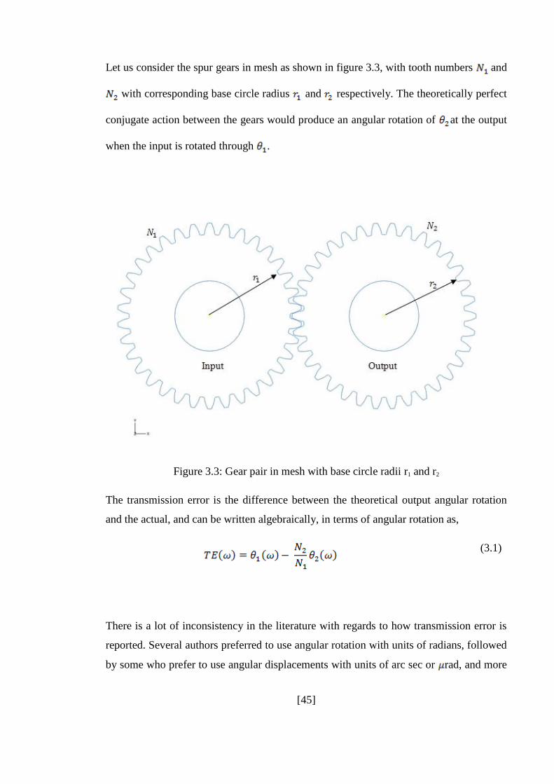
[45]
Let us consider the spur gears in mesh as shown in figure 3.3, with tooth numbers and
with corresponding base circle radius and respectively. The theoretically perfect
conjugate action between the gears would produce an angular rotation of at the output
when the input is rotated through .
Figure 3.3: Gear pair in mesh with base circle radii r1 and r2
The transmission error is the difference between the theoretical output angular rotation
and the actual, and can be written algebraically, in terms of angular rotation as,
(3.1)
There is a lot of inconsistency in the literature with regards to how transmission error is
reported. Several authors preferred to use angular rotation with units of radians, followed
by some who prefer to use angular displacements with units of arc sec or rad, and more
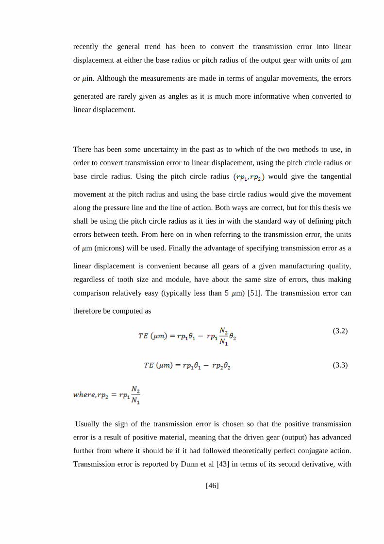
[46]
recently the general trend has been to convert the transmission error into linear
displacement at either the base radius or pitch radius of the output gear with units of m
or in. Although the measurements are made in terms of angular movements, the errors
generated are rarely given as angles as it is much more informative when converted to
linear displacement.
There has been some uncertainty in the past as to which of the two methods to use, in
order to convert transmission error to linear displacement, using the pitch circle radius or
base circle radius. Using the pitch circle radius would give the tangential
movement at the pitch radius and using the base circle radius would give the movement
along the pressure line and the line of action. Both ways are correct, but for this thesis we
shall be using the pitch circle radius as it ties in with the standard way of defining pitch
errors between teeth. From here on in when referring to the transmission error, the units
of m (microns) will be used. Finally the advantage of specifying transmission error as a
linear displacement is convenient because all gears of a given manufacturing quality,
regardless of tooth size and module, have about the same size of errors, thus making
comparison relatively easy (typically less than 5 m) [51]. The transmission error can
therefore be computed as
(3.2)
(3.3)
Usually the sign of the transmission error is chosen so that the positive transmission
error is a result of positive material, meaning that the driven gear (output) has advanced
further from where it should be if it had followed theoretically perfect conjugate action.
Transmission error is reported by Dunn et al [43] in terms of its second derivative, with
[47]
units of radians/sec2, because the measurement of transmission error was performed in
terms of angular acceleration.
Even though the transmission error is known to be time dependent and relative to the
respective position of the gear teeth in contact, it is almost always reported as a single
peak-to-peak value by Houser et al [35]. Other researchers look into the Fourier analysis
of transmission error and identify the problem in the gear system by the frequency
content in the data. If there is a profile error on one of the tooth, it will show up on the
frequency spectrum at the tooth frequency and its harmonics, as the rest of the frequency
response from tooth to tooth will be consistent.
Some authors [38, 52] use the frequency spectrum to identify ghost frequencies in gear
systems, as these will display themselves at other frequencies too. Ghost frequencies are
usually the result of manufacturing errors and can be rectified by better quality checks
and tighter tolerances.
3.5.2 Types of transmission error
There are a few types of transmission errors that are frequently referred to in the
literature and they vary in small measures from one another. These are:
3.5.2.1 Manufacturing transmission error
This is quite simple to understand, as the gear tooth geometry directly influences the
angular position of the output gear for a given position of the input gear, so that any
change in the tooth contact point would give rise to transmission error. This change being
due to the manufacture of the gears is called manufacturing transmission error. This is
the only kind of transmission error that is a measure of a single gear error. Generally, the
transmission error relates to the meshing of two gears, and hence can be said to be the
sum of the respective transmission errors of the individual gears [42]. The
manufacturing transmission error (MTE) is measured under no load or lightly loaded
[48]
conditions [9] and can be used to test the accuracy of gears on a production line, as used
on single flank machines.
3.5.2.2 Static transmission error
When two gears mesh under the presence of low load conditions, the gear teeth deform
elastically along with the gearbox casing, bearing, and shafts. Hence it can be supposed
that the transmission error under the influence of low load is the static transmission error
(STE), and also takes into consideration stiffness of all the components in the system.
The static transmission error is measured at low speeds to avoid the dynamic effects of
the system.
The teeth of the gear pair experience deformation due to loading in the form of bending
and contact between them, making up the mesh stiffness. As the gears rotate through the
mesh, the numbers of teeth in mesh changes depending on the contact ratio of the gears
and therefore also influencing the mesh stiffness between the gear teeth. There have been
several approaches to approximate the variable mesh stiffness in the static case,
Blankenship and Singh [53] suggest that the stiffness might also depend on the mesh
load, and Mark [42] has defined the stiffness in terms of an area integral over the contact
zone, while taking into account the local surface irregularities.
3.5.2.3 Kinematic transmission error
The kinematic transmission error (KTE) is a derivation of the MTE, which takes into
consideration the asperities present on the tooth surfaces. Asperities are local unevenness
of the surface, roughness and ruggedness that cannot be seen with the naked eye. When
two surfaces with such asperities come into contact these asperities deform until the
contact area increases and can support the load.
Blankenship and Singh [53] investigate this type of subtle elastic deformations on the
gear teeth surfaces that take place under low load. They suggest that under low load, the

[49]
contact deformations of the teeth are averages of the local deformation of the asperities
present on the working surfaces. As the asperities are not an intentional design feature,
they can be attributed to a manufacturing error. Practically, there is very small difference
between the MTE and KTE as the MTE is simply a special case of KTE under no load.
3.5.2.4 Dynamic transmission error
The concept of dynamic transmission error recognises that the gear system has
components with masses and variable stiffness. By taking into consideration the masses
of the gears, and their rotations, the inertial forces of the system causes dynamic mesh
forces. Gear designers for over a hundred years have been adjusting their gear life
calculations using the dynamic factor. The dynamic factor is a ratio of the dynamic load
to the static load as a result of tooth geometry errors.
Özgüven and Houser [7] provide a history of dynamic factor work as an introduction to a
historical review of mathematical models used in gear dynamics. While the dynamic
factor does not accurately represent the dynamics of the tooth mesh, it shows that the
dynamic loading in the mesh is a result of the static transmission error. This static
transmission error is the source of excitation for the dynamic transmission error.
Dynamic transmission error is speed dependent and can be mathematically represented
by multiplying static transmission error by a transfer function [18].
3.6 Methods to estimate transmission error
While dynamic transmission error is the transmission error type most closely related to
gear noise, it of course is the most difficult to obtain, either by analysis or measurement.
Since dynamic transmission error is excited by static transmission error, it is fruitful to
reduce noise by addressing static transmission error. The alternating component of static
transmission error is reduced by specifying tooth modifications that compensate for the
stiffness variation.

[50]
By plotting transmission error curves for multiple loads on the same graph, one can
easily see how load affects transmission error. This plot is called a Harris Map (Fig. 3.4).
Munro and Houser [38] show how gear geometry can be used to synthesize no load
transmission error curves. Loaded transmission errors can be predicted using software
such as LDP (Load Distribution Program) from Ohio State University’s Gear Dynamics
and Gear Noise Research Laboratory [59]. Most transmission error analysis tools
compute static transmission error.
Figure 3.4: Harris map showing effect of varying load on teeth deflection. [51]
Houser, et al. [17] showed that sound power measurements (sum of harmonics and
sidebands) correlated well with predicted transmission error in parallel axis arrangement.
They compared spur, helical and double helical (herringbone) gears. They tested
conventional and high contact ratios and other tooth modifications. Transmission error
was determined by analysis using LDP. They also say that the transmission error is less
sensitive to load at higher contact ratios.
[51]
3.7 Mesh stiffness modelling
Over recent decades, many attempts have been made by numerous authors to set up
mathematical and numerical models aimed at simulating the dynamic behaviour of gears
[11–15]. The mathematical formulations range from single-degree-of freedom (SDOF)
models to finite element three-dimensional (3D) ones. In SDOF the mesh stiffness can
either be determined on the basis of simplified assumptions or by using the results of
more refined finite-element simulations but virtually all gear dynamic models consider
that transmission error (TE) and variations in mesh stiffness are the primary sources of
excitation. It is clear from the previous chapters that as the gears rotate, the number of
teeth pairs in contact through the mesh cycle and their points of contact vary and
therefore the “mesh stiffness” varies with the rotation. The mesh stiffness (although
strictly speaking it is the teeth stiffness of the teeth in contact) varies due to geometrical
imperfections of the teeth, acceleration/deceleration of gears due to impact and changing
contact ratios of the gears. This is one of the main reasons TE of gear pairs in not a single
value, but rather a continuous variable through gear rotations, and should be measured at
different relative positions of the gear with its mesh cycle.
From the gear designer’s point of view, the definition of tooth modifications for low-
noise gears also relies on the minimization of transmission error variations [16–18].
However, most of the theoretical background stems from single-degree-of-freedom
(SDOF) torsional models [19] and very little attention has been given to the validity and
limits of the concept of transmission errors as main excitation sources. As previously
stated, TE is considered to be one of the main causes of gear noise and vibration, and
numerous works have been published on gear TE. [11, 17, 18, 20 – 23]
The mesh stiffness model forms the basis for a dynamic model of a gear pair. In early
research, the mesh stiffness of gear teeth was considered to be constant. Iwatsubo and
Kawai [93] studied the lateral and torsional vibrations of geared rotors, mainly
considering the effect of the periodic variation of the mesh stiffness. The combined mesh
stiffness of the two gears in mesh varies with the meshing position as the teeth rotate
within the mesh cycle. In particular, the mesh stiffness decreases and increases
[52]
dramatically as the meshing teeth change from the double pair of teeth in contact, to the
single pair of teeth in contact. The combined mesh stiffness is defined as the ratio
between the torsional load and the angular rotation of the gear body.
The mesh stiffness associated with elastic tooth bending varies as the number of teeth in
contact changes. The parametric excitation from the time-varying mesh stiffness causes
instability and severe vibration under certain operating conditions. Experiments [41, 42]
have demonstrated the large amplitude vibration induced by parametric instability where
the gear mesh frequency equals twice the natural. Furthermore, mesh stiffness variation
directly affects tooth deflections and transmission error. Kamaya [18] has aptly
summarised that mesh stiffness along with transmission error are the primary causes of
gear noise and vibration.
Frolov and Kosarev [95] highlight the importance of mesh stiffness under variable load
as one of the primary causes of gear vibrations, along with pitch error and profile error.
In their generalized vibroexcitation gear model, they go on to disprove the collision
model, which specifies that edge impact is the primary causes of TE. Frolov and Kosarev
conclude that the factors causing gear vibration can generally be eliminated by profile
modifications, adjustment of contact ratio and high-precision manufacture of gears.
3.8 Gear dynamic modelling
The literature suggests that many different models have been developed in the past sixty
years. In effect the first mass-spring approach to gear dynamics was created by Tuplin
[54] and intensive studies were conducted by Harris [6], Munro and Gregory [5, 11] in
the sixties. An interesting literature overview can be found in [7], where the
mathematical models used in gear dynamics were classified by considering: the
evaluation of simple dynamic factor, tooth compliance, gear dynamics, geared motor
dynamics, and torsion vibration. This paper shows how the interest on gear vibrations
grew up continuously from the seventies.
[53]
In the eighties important contributions were given by Bahgat et al. [94], who presented a
dynamic procedure based on Hertz impact formula for two cylinders in contact, by Yang
et al. [55] who proposed two different models to take into account energy dissipation,
hertzian damping and tooth friction, and by Umezawa et al [56], who developed
approximate equation to simulate rotational vibrations of both spur and helical gears.
In the last twenty years, most of the dynamic models were focused on non-linear aspects.
Kahraman and Singh [57] considered the effect of backlash and time varying mesh
stiffness using harmonic balance method and digital simulation. A similar model was
developed by Theodossiades and Natsiavas [58] who predicted chaotic behaviour by
means of numerical methods. Ozguven [62] extended the nonlinear spur gear model by
considering the effects of both shaft and bearing dynamics. Cai and Hayashi [29]
proposed a linear approximation for a pair of spur gears and compared the analytical
solution with the numerically calculated result by the nonlinear equation.
All previous papers agree in considering the following sources of vibrations for gears
system: torsion resonance, impulsive or cyclic fluctuations in drive torque, gear mesh,
transmission error, local component vibration responses and fluctuations in the output
torque demand. The concept of a vibrating system made of two gears is generally
modelled through two wheels linked by the teeth mesh stiffness. In its simplest form, this
model can simulate the classical linear resonance, i.e. the resonant frequency of the
system. However, more complex phenomena such as parametric instabilities can be an
important source of noise.
3.9 Non-linear finite element analysis of gear pairs
Analyses of gears under several conditions using the finite element method (FEM) have
already been reported in the literature [13]. Indeed, these types of analysis are fast
[54]
becoming the focus of increasing attention as more sophisticated programs with higher
calculations capabilities and accuracy are developed. Some of the pioneering
developments in analytical methods have resulted from using FEM - derived data that
included more complete models of the system components and geometry. Initially,
models were analysed consisting only the teeth in mesh, but it is now becoming common
to include the remaining teeth, gear body, shaft system, and bearings [89, 90].
Among the early work in finite element simulations, the photo-elastic experiments used
to evaluate stress distributions were replaced by the finite element method as a means of
investigating the effect that design parameter changes have upon the bending stress [82].
If the finite element method can be shown to accurately model gear tooth behaviour then
this course of action would be preferable to the use of the approximated semi-empirical
formulae as advocated by the majority of the standards. In the research work carried out
by Andrews [83] the finite element method has been used for predicting the fillet stress
distribution experienced by loaded spur gears. The location of the finite element model
boundary and the element mesh density are investigated and compared with
corresponding photo-elastic experiments, and showed good correlation with the photo-
elastic experiments on spur gear teeth carried out by Allison and Hearn [84].
Most of the existing work on gear models are carried out by utilising gap elements to
simulate the gear surface contact behaviour and estimated the contact pressures and
deformations. Gap elements can be used to define contact between two nodes when there
are either in contact (closed) or separated (open) with respect to particular directions and
separation conditions. Although the gap elements are defined in three dimensions only,
they can still be used in two dimensional models.
To use the gap element method, the location of the contact must first be calculated using
classical Hertzian theory as discussed further on in this Thesis (Chapter 4). The other
limitations of using gap elements are that they usually allow relatively small sliding
between the contact surfaces. To understand the loaded gear multi-tooth rolling/sliding
contact behaviour, the advanced general multiple surfaces to surfaces contact technique
is used. This technique can simulate the rolling/sliding and separation without requiring
the exact location of the contact area as required by the gap element method.
[55]
There are three main sources of non-linearity when considering structural mechanics
simulations. These nonlinearities are due to the material, geometry and contact non-
linearity, which will be covered in further detail in Chapter 5.
Contact conditions are a special class of discontinuous constraint, allowing forces to be
transmitted from one part of the model to another only when the two surfaces are in
contact. On separation, no constraint is applied to the two surfaces. The analysis has to be
able to detect when two surfaces are in contact and apply the contact constraints
accordingly. Similarly, the analysis must be able to detect when two surfaces separate
and remove the contact constraints. The contact algorithm in Abaqus [28], is built around
the Newton-Raphson technique.
In Abaqus the Newton-Raphson technique is used to examine the state of all contact
interactions at the start of each increment to establish whether slave nodes are open or
closed. A constraint will be applied for each closed node and constraints are removed
from any node where the contact state changes from closed to open. Iteration is then
carried out and the configuration of the model is updated using the calculated corrections.
Before checking for equilibrium of forces or moments, any changes in the contact
conditions at the slave nodes are checked first. Any node where the clearance after the
iteration becomes negative or zero has changed status from open to closed. Any node
where the contact pressure becomes negative has changed status from closed to open.
The contact constraints are modified to reflect the change in contact status after the first
iteration and a second iteration is tried. The procedure is repeated until the iteration is
completed with no changes in contact status. This iteration becomes the first equilibrium
iteration and the normal equilibrium convergence checks are performed. The entire
process is repeated until convergence is achieved.
Literature published on the effect of varying contact conditions in gear tooth interactions
through finite element method, on the perceived transmission error from gear pair models
is quite sparse. In a recent study by Li and Kahraman [86] a numerical non-Newtonian
contact model of an involute spur gear tooth is developed with respect to various contact
parameters such as surface velocities, normal load and radii of curvature.
[56]
In the majority of researches, modelling the gear using the finite element method requires
the domain over which the results were to be calculated to be first established. This
domain of interest is obtained intuitively from the physical geometry of the structure, and
in the case of gear teeth the area of interest could be approximated by a single gear tooth
or be extended to include the whole gear. Andrews [83] uses the approach of modelling a
single gear tooth due to computational inefficiencies to evaluate the stress distribution in
the fillet of a loaded tooth model. This will be one of the outcomes form this Thesis and
will be discussed in detail in Chapter 7.
3.10 Optimisation of gears
Optimisation of a design is the process by which an objective function is defined with
respect to several fixed parameters along with other design variables, and re-evaluated to
improve the target value of the function. There are many different ways to optimise and
also different range of optimisation processes such as one, two or multiple parameter
optimisation.
3.10.1 Optimisation criteria
Optimisation is possible in any aspect of mechanical design if one introduces stringent
criteria by which the design must satisfy its functions and can then be developed with
respect to what is expected from it. This introduces the concept of “needs analysis”,
which summarises the needs to be met by the design being developed. In the case of the
spur gear pair, the “needs analysis” would specify the following conditions:
a. The spur gear pair must be strong enough to withstand the applied forces without
failing.
b. The spur gear pair must be capable of carrying the maximum possible torque for
the specific application. In the case of the spur gear pair being modelled in this
Thesis, the maximum torque to be face will be 10000Nmm, which will be
validated in the following chapter.
c. One of the pertinent functions of the spur gear pair with regards to this work has
to do with the noise generated due to the vibration generated from the gears
meshing. This is summarised by Smith [51] showing that the relationship between
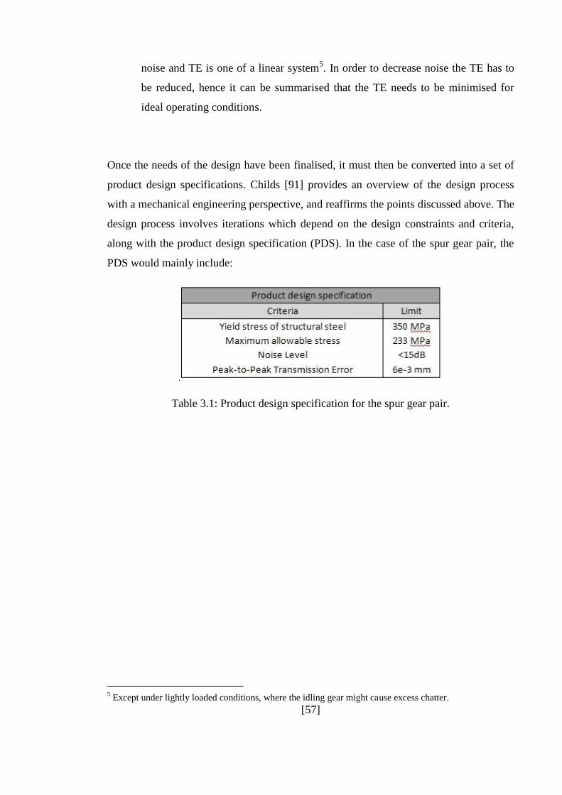
[57]
noise and TE is one of a linear system5. In order to decrease noise the TE has to
be reduced, hence it can be summarised that the TE needs to be minimised for
ideal operating conditions.
Once the needs of the design have been finalised, it must then be converted into a set of
product design specifications. Childs [91] provides an overview of the design process
with a mechanical engineering perspective, and reaffirms the points discussed above. The
design process involves iterations which depend on the design constraints and criteria,
along with the product design specification (PDS). In the case of the spur gear pair, the
PDS would mainly include:
Table 3.1: Product design specification for the spur gear pair.
5 Except under lightly loaded conditions, where the idling gear might cause excess chatter.
[58]
4. SPUR GEAR METHODOLOGY AND DATA
VALIDATION
4.1 Introduction
In this chapter the details of spur gear design with respect to performance characteristics
shall be discussed. The main aspects of stress formulae, design limits, strength and
durability calculations shall be examined. In the previous chapters the task of identifying
the correct gear choice was the main objective, while this chapter will deal with the
detailed work involved in designing a spur gear. This preliminary design work involves
consideration of the level of stresses the gear will come across, an estimation of the
approximate gear size and consideration of the operating limits for the chosen design.
The purpose of the calculations are to enable the gear designer to choose the right
variables in terms of module, tooth thickness, tooth size and base radius, for the relevant
application. In this project however, the calculations are intended to give the reader a
general understanding of the basic information needed to design a gear, whilst keeping in
mind that the final object of creating an automated profile generation tool will take care
of the choice of variables comparable to actual working spur gear designs. The latter part
of this chapter will then lead into the calculations used to derive the spur gear involute
profile for the PYTHON scripts, as described in the next chapter.
4.2 Lewis’s formula for gear strength calculation
The first problem faced by a gear designer is to find a design that will be able to carry the
required power of the application. It is needless to say that the gear designed should be
accurate enough, strong enough and big enough to perform the required job. Usually,
failure by bending occurs when significant tooth stress equals or exceeds the yield
strength or endurance strength of the material.
[59]
However, it has to be said that the stresses calculated using gear design formulae will not
necessarily be true stresses when compared to experimental results. This is mainly due to
the gear tooth being idealised to a cantilever beam, and formulae being derived from this
approximation. Any assumptions used to permit calculations of stress in gear teeth
usually do not take into consideration effects such as stress concentrations, residual
stress, misalignment and tooth errors.
Another factor making comparison between theoretical and experimental stress more
difficult is the loading on the gear teeth. Even if the load that the gear teeth can be subject
to is known, it is highly unlikely that this load is shared evenly between two or more
pairs of teeth when meshing and also being evenly distributed across their face width.
Errors in tooth spacing normally upset the load sharing between teeth causing
accelerations and decelerations which cause a dynamic overload of the gear pair system.
Even taking into consideration the difficulties faced in calculating true stresses, gear
stress formulae are valuable and a necessary design tool. The formulae can be used to
estimate how well the new gear being designed can perform, whist keeping in mind that
it can only provide an estimate of the performance of the new gear design. When
designing a new gear, the designer must take into consideration the stress limits,
temperature limits and oil-film-thickness limits. Besides these first-order requirements,
one must satisfy secondary considerations like vibration, noise and environmental
effects.
In order to better understand how these relate to the concept of gear design, an
introduction to the well known Lewis bending equation will be an apt starting point.
In 1892, Wilfred Lewis put forward an equation for approximating the bending stress in
gear teeth, where the teeth form was relative to the calculation, and this equation is still
very much relevant today, forming the basis for most gear designs. Essentially the gear
tooth is similar to a stubby cantilever beam (Figure 4.1) that has tensile stress at the base
of the loaded side and compressive stress on the opposite side. Most commonly, gear
teeth fail by crack propagation at the base of the tooth on the loaded side on the tooth.
This ability of the gear teeth to resist tooth breakage is usually referred to as their beam
strength or flexural strength. Lewis was the first to calculate this flexural strength of gear
teeth to a very close degree of accuracy.
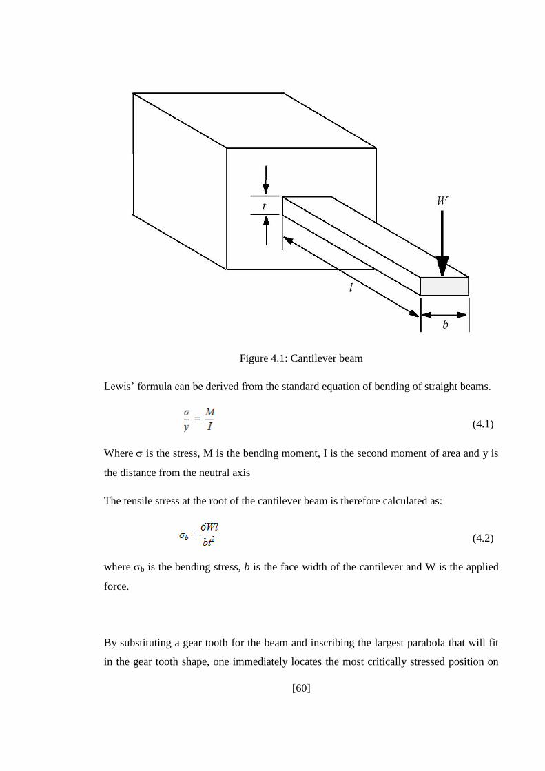
[60]
Figure 4.1: Cantilever beam
Lewis’ formula can be derived from the standard equation of bending of straight beams.
(4.1)
Where is the stress, M is the bending moment, I is the second moment of area and y is
the distance from the neutral axis
The tensile stress at the root of the cantilever beam is therefore calculated as:
(4.2)
where b is the bending stress, b is the face width of the cantilever and W is the applied
force.
By substituting a gear tooth for the beam and inscribing the largest parabola that will fit
in the gear tooth shape, one immediately locates the most critically stressed position on
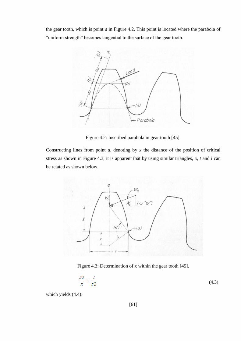
[61]
the gear tooth, which is point a in Figure 4.2. This point is located where the parabola of
“uniform strength” becomes tangential to the surface of the gear tooth.
Figure 4.2: Inscribed parabola in gear tooth [45].
Constructing lines from point a, denoting by x the distance of the position of critical
stress as shown in Figure 4.3, it is apparent that by using similar triangles, x, t and l can
be related as shown below.
Figure 4.3: Determination of x within the gear tooth [45].
(4.3)
which yields (4.4):
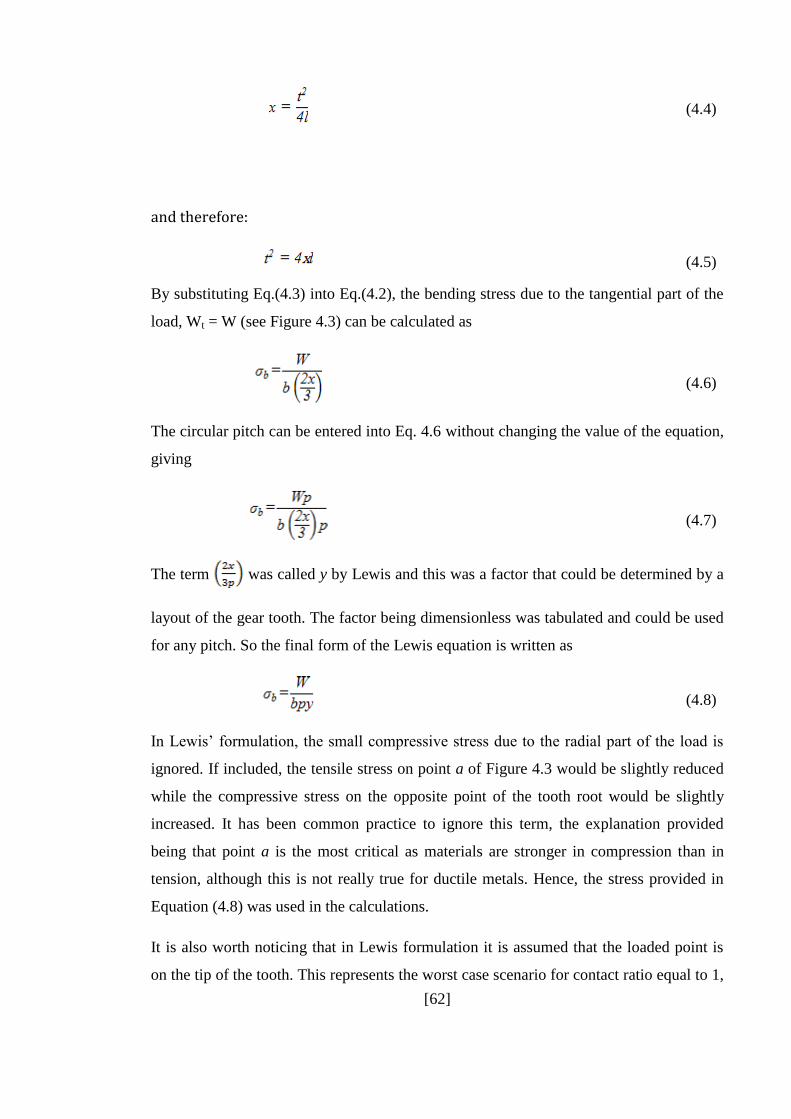
[62]
(4.4)
and therefore:
(4.5)
By substituting Eq.(4.3) into Eq.(4.2), the bending stress due to the tangential part of the
load, Wt = W (see Figure 4.3) can be calculated as
(4.6)
The circular pitch can be entered into Eq. 4.6 without changing the value of the equation,
giving
(4.7)
The term was called y by Lewis and this was a factor that could be determined by a
layout of the gear tooth. The factor being dimensionless was tabulated and could be used
for any pitch. So the final form of the Lewis equation is written as
(4.8)
In Lewis’ formulation, the small compressive stress due to the radial part of the load is
ignored. If included, the tensile stress on point a of Figure 4.3 would be slightly reduced
while the compressive stress on the opposite point of the tooth root would be slightly
increased. It has been common practice to ignore this term, the explanation provided
being that point a is the most critical as materials are stronger in compression than in
tension, although this is not really true for ductile metals. Hence, the stress provided in
Equation (4.8) was used in the calculations.
It is also worth noticing that in Lewis formulation it is assumed that the loaded point is
on the tip of the tooth. This represents the worst case scenario for contact ratio equal to 1,
[63]
which was approached in most cases at Lewis’ times. With higher contact ratios, the
assumption of having the force applied on the tip of the tooth is conservative.
Some gear designers prefer to work using module or diametral pitch instead of circular
pitch, while making stress calculation. In terms of the module, the Lewis formula can be
modified to
(4.9)
where p = m, Y = y and m is the module of the gear as shown in Eq. 2.8 and is related
to the circular pitch by a factor of .
4.3 Modified Lewis formula
In the current engineering practice some factors are introduced in Lewis’ formula
because a gear system has to be designed to withstand the rigours of the application it has
been developed for. The formula is therefore modified as follows:
(4.10)
where is the tangential load, is the overload factor, is the dynamic factor, is
the size factor, is the face width of the tooth, is the load distribution factor, is
the rim thickness factor, is the geometry factor for bending strength. These factors are
discussed in more detail below.
4.4 Dynamic factor, Kv
The dynamic nature of the problem leads to an amplification of the transmitted load. In
general, the faster the gears are run, the more shock due to the tooth errors and more
dynamic effects due to the imbalance and torque variations are present in the driving and
driven gears. Lewis allowed for this situation by reducing the safe working stress as the
pitch-line velocity was increased.
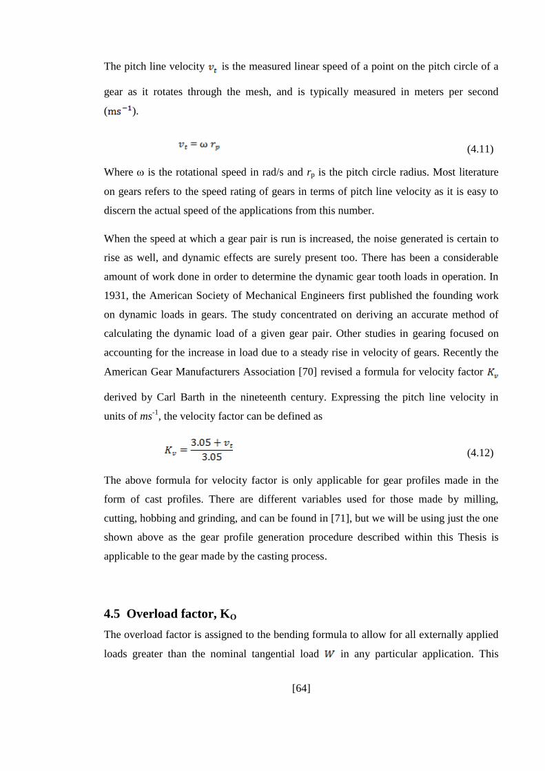
[64]
The pitch line velocity is the measured linear speed of a point on the pitch circle of a
gear as it rotates through the mesh, and is typically measured in meters per second
( ).
(4.11)
Where is the rotational speed in rad/s and rp is the pitch circle radius. Most literature
on gears refers to the speed rating of gears in terms of pitch line velocity as it is easy to
discern the actual speed of the applications from this number.
When the speed at which a gear pair is run is increased, the noise generated is certain to
rise as well, and dynamic effects are surely present too. There has been a considerable
amount of work done in order to determine the dynamic gear tooth loads in operation. In
1931, the American Society of Mechanical Engineers first published the founding work
on dynamic loads in gears. The study concentrated on deriving an accurate method of
calculating the dynamic load of a given gear pair. Other studies in gearing focused on
accounting for the increase in load due to a steady rise in velocity of gears. Recently the
American Gear Manufacturers Association [70] revised a formula for velocity factor
derived by Carl Barth in the nineteenth century. Expressing the pitch line velocity in
units of ms-1
, the velocity factor can be defined as
(4.12)
The above formula for velocity factor is only applicable for gear profiles made in the
form of cast profiles. There are different variables used for those made by milling,
cutting, hobbing and grinding, and can be found in [71], but we will be using just the one
shown above as the gear profile generation procedure described within this Thesis is
applicable to the gear made by the casting process.
4.5 Overload factor, KO
The overload factor is assigned to the bending formula to allow for all externally applied
loads greater than the nominal tangential load in any particular application. This

[65]
applies to our example of internal combustion engines, where the torque fluctuates due to
the firing of different cylinders within the engine. The overload factor can be chosen
depending on the required application as shown in Table 4.1.
Table 4.1: Table of Overload factors, [74]
4.6 Size factor, KS
The size factor for the gear set reflects the non-uniformity of material properties due to
change in size. This usually depends on the tooth size, diameter of gear and face width
among other factors. If the face width of the gear is chosen as 3 to 5 times the circular
pitch, then there will be no discernable detrimental size effect, and hence the AGMA
have identified and suggested that should be used. Alternatively, this value can be
calculated for cases where there are big detrimental size effects [71].
4.7 Load distribution factor, KH
Distribution of load across the line of contact in non-uniform and is accounted for by the
load distribution factor. The general formula is
(4.13)
where, is the distribution factor for face width effects and is the distribution
factor for the transverse effects. If the gear teeth mesh reasonably well, the effect of
is relatively small compared to the larger coefficient . ISO standards [72, 73] are
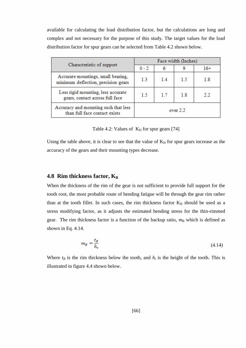
[66]
available for calculating the load distribution factor, but the calculations are long and
complex and not necessary for the purpose of this study. The target values for the load
distribution factor for spur gears can be selected from Table 4.2 shown below.
Table 4.2: Values of KH for spur gears [74]
Using the table above, it is clear to see that the value of KH for spur gears increase as the
accuracy of the gears and their mounting types decrease.
4.8 Rim thickness factor, KB
When the thickness of the rim of the gear is not sufficient to provide full support for the
tooth root, the most probable route of bending fatigue will be through the gear rim rather
than at the tooth fillet. In such cases, the rim thickness factor KB should be used as a
stress modifying factor, as it adjusts the estimated bending stress for the thin-rimmed
gear. The rim thickness factor is a function of the backup ratio, mB which is defined as
shown in Eq. 4.14.
(4.14)
Where tR is the rim thickness below the tooth, and ht is the height of the tooth. This is
illustrated in figure 4.4 shown below.
[67]
Figure 4.4: Rim thickness factor, KB [71]
The rim thickness factor is thus defined as
(4.15)
In our gear pair case, the backup ratio, mB is sufficiently bigger than 1.2, therefore the
rim thickness factor, KB, for all cases investigated will be 1.
4.9 Expressing the load as a function of the transmitted power
The gear set must handle a specified power at a given input speed. Given the power, the
torque acting on the gear is first calculated, and then converted to a tangential force
acting at the pitch diameter. The input torque of the driving gear T1, expressed in Nm, is
given by
(4.14)
where n1 is the rotational speed in RPM and, P is the power in kilowatts and
. The tangential load can then be calculated as
(4.15)
[68]
where W is the tangential load expressed in Newton and dp1 is the driving gear pitch
circle diameter expressed in millimetres.
4.10 Evaluation of the contact stress
The contact stress can be determined by the following formula [71]
(4.16)
where is the surface condition factor, is the geometry factor for pitting, is the
pitch diameter of the gear and is an elastic coefficient.
4.11 Gear design using the expressions for bending and contact stress
Before using the formulas for the bending and contact stress to validate the cases studied
later in chapters 6 and 7, it is worth noting that the calculations for gear tooth strength
have become complex in many ratings standards of the American Gear Manufacturing
Association (AGMA), International Standards Organisation (ISO) and other trade
groups. Following the various standards around the world can be very tricky and the
worst possible case can be a mix up between two standards. In this research, AGMA
standards with metric units have been used throughout.
In the case of our spur gear pair, the data needed to start producing the spur gear
geometry come from an automotive passenger car background. The power required for a
typical gearbox in an automotive operating cycle varies depending on the load. Figure
4.5 shows the respective torque curves for spark ignition (SI) and compression ignition
(CI) engines with respect to engine speeds. As can be seen, the torque range for an SI
engine covers a much broader range of speeds than a CI engine and does not go over 150
Nm at peak velocity of 3500 rpm as compared to 350Nm for the CI engine at 1700 rpm
[75].
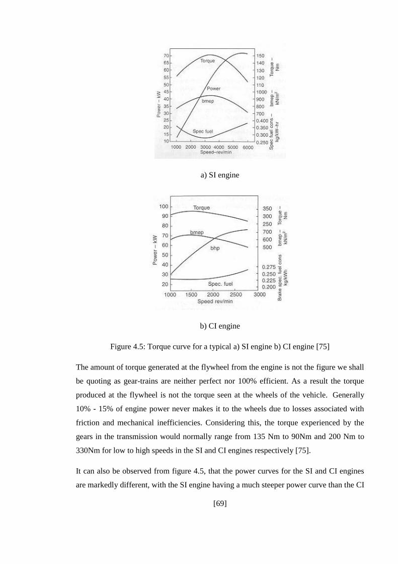
[69]
a) SI engine
b) CI engine
Figure 4.5: Torque curve for a typical a) SI engine b) CI engine [75]
The amount of torque generated at the flywheel from the engine is not the figure we shall
be quoting as gear-trains are neither perfect nor 100% efficient. As a result the torque
produced at the flywheel is not the torque seen at the wheels of the vehicle. Generally
10% - 15% of engine power never makes it to the wheels due to losses associated with
friction and mechanical inefficiencies. Considering this, the torque experienced by the
gears in the transmission would normally range from 135 Nm to 90Nm and 200 Nm to
330Nm for low to high speeds in the SI and CI engines respectively [75].
It can also be observed from figure 4.5, that the power curves for the SI and CI engines
are markedly different, with the SI engine having a much steeper power curve than the CI
[70]
engine but both engines hitting maximum peak power of approximately 75 – 80 kW at
their respective maximum speeds (5500 rpm for SI and 2700 rpm for CI).
Taking all of this into consideration, it is possible to evaluate the operating conditions
that a typical gear box might face in operation. In the case of an SI engine, it will
experience maximum torque of 135Nm in the mid-range of its speed, approximately at
4000 rpm and between 50 and 55 kW power.
In the case of our gear pair model, the 2D model is based on plane strain principles and
as such has a maximum thickness of 1mm in the ABAQUS FE model. In automotive
gear boxes, the spur gear pairs that are commonly used, have face widths ranging from
10mm to 25mm depending on the power output experienced by the gear box. Taking a
maximum face width value of 25mm and torque of 150Nm, it would be possible to
approximate the maximum (and minimum) loads faced by the gear pairs in action as
shown below:
Torque acting on normal face width = 150Nm = 150000Nmm
Normal spur gear face width = 25mm
Face width of Abaqus spur gear = 1mm
Torque needed for Abaqus spur gear model = T1
(4.17)
For the case of our spur gear pair, for an automotive passenger car transmission, the less
rigid mounting gears with full face contact is chosen. In the Abaqus model that will be
defined in the Chapters 5 and 6, a plane strain model will be used; hence the face width
value of 1mm is the pre-selected default and is deemed sufficient. From Table 4.2, the
value of 0 – 2 inches will be sufficient for our purposes.
[71]
5. AUTOMATED SPUR GEAR PROFILE
GENERATION METHODOLOGY USING
PYTHON SCRIPTS IN ABAQUS
In this chapter a procedure to model the geometry of a pair of spur gears in the finite-
element code ABAQUS and to input material properties, loading and boundary
conditions for static and dynamic analyses is presented. The case is considered in which
the angular velocity is prescribed for the driving gear and the torque is assigned for the
driven gear. The procedure has been implemented into a Python script so that the user
only has to input the macro-geometrical parameters of the gear, as well as the prescribed
angular velocity and torque, and run the analysis with the click of a button. The
advantages of this fully automated procedure will be particularly apparent in Chapter 8,
where an automatic optimisation analysis is conducted with an algorithm implemented in
Matlab which calls the developed procedure at every iteration.
Gear designers are faced with having to compute accurate mathematical models of gears,
and most three dimensional solid modelling programs cannot easily accommodate the
true involute geometry used to generate the tooth profile, other than by approximating to
a small number of finite points. As a result, existing methods for gear generating involve
the following procedures:
Establish the mathematical model of the gear drives according to the
manufacturing process and gear meshing theory
Export the calculated surface data points into a CAD package, construct the
surface data points into the gear surface, and trim the surface according to the
design parameters. Typically the gear geometry is generated solely from a CAD
tool owing to the geometry generation limitations of the currently available
commercial FEA software
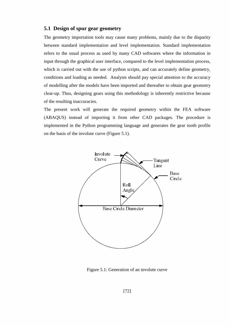
[72]
5.1 Design of spur gear geometry
The geometry importation tools may cause many problems, mainly due to the disparity
between standard implementation and level implementation. Standard implementation
refers to the usual process as used by many CAD softwares where the information in
input through the graphical user interface, compared to the level implementation process,
which is carried out with the use of python scripts, and can accurately define geometry,
conditions and loading as needed. Analysts should pay special attention to the accuracy
of modelling after the models have been imported and thereafter to obtain gear geometry
clear-up. Thus, designing gears using this methodology is inherently restrictive because
of the resulting inaccuracies.
The present work will generate the required geometry within the FEA software
(ABAQUS) instead of importing it from other CAD packages. The procedure is
implemented in the Python programming language and generates the gear tooth profile
on the basis of the involute curve (Figure 5.1).
Figure 5.1: Generation of an involute curve

[73]
This method is highly accurate geometrically and hence avoids the small errors that
accumulate when using standard implementation. This accurate gear generation method
provides researchers with a powerful tool for investigating the effects of gear tooth
surface micro-geometry modifications.
The layout and geometry for a pair of meshing spur gears can be determined by the
procedure outlined in this chapter. It should be noted that gears are commonly available
as standard items from specialist manufactures and suppliers and need not necessarily be
designed from scratch. In the case of the research being carried out, it is imperative that
the design process for the gears can be replicated and gear geometry is as accurate as
possible.
The first step would be to finalise the gear pair geometry required for the specific
application. In the chapter we will develop the automation code to focus our attention on
a pair of spur gears of equal diameter and number of teeth, which can then be modified as
required to generate spur gear pairs of differing geometry. The gear pair geometry data is
shown below:
Gear Geometry Values
Driver and driven gears 34 teeth
Pressure angle, θ 20°
Module, m 2
Centre distance, d 50 mm
Gear pair ratio, R1:R2 1:1
Number of teeth, N1 34
Sector of involute curve 30°
Division of sector, Npoints 10
Tip relief, Addmodmax 50 μm
Table 5.1: Spur gear geometry data
The first step is to calculate the pitch circle diameters for both gears and construct the
respective pitch circles tangential to each other.
(5.1)
(5.2)

[74]
The module of the gear pairs will then be defined in order to construct the addendum and
dedendum radii. m1 and m2 are defined as shown in Eq. 5.3.
(5.3)
Omega, is defined next which will be later used to define the rotation matrix that is
used to plot the points on the base radius in terms of the involute curve. ω1 and ω2 are
defined as shown in Eq. 5.4.
(5.4)
The base radius, rb is defined using the pitch circle and the pressure angle of the
respective gears and is the starting point of the involute curve. (Figure 5.2).
(5.5)
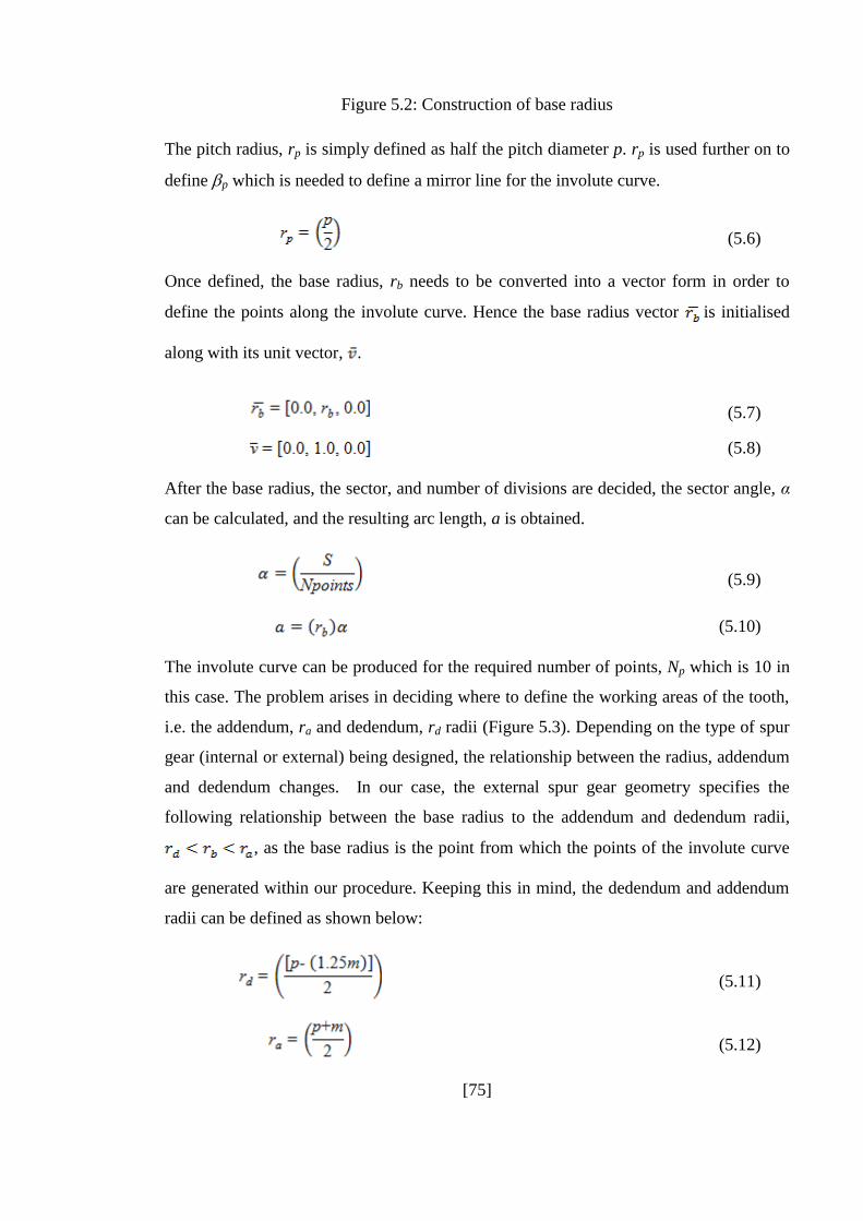
[75]
Figure 5.2: Construction of base radius
The pitch radius, rp is simply defined as half the pitch diameter p. rp is used further on to
define p which is needed to define a mirror line for the involute curve.
(5.6)
Once defined, the base radius, rb needs to be converted into a vector form in order to
define the points along the involute curve. Hence the base radius vector is initialised
along with its unit vector, .
(5.7)
(5.8)
After the base radius, the sector, and number of divisions are decided, the sector angle, α
can be calculated, and the resulting arc length, a is obtained.
(5.9)
(5.10)
The involute curve can be produced for the required number of points, Np which is 10 in
this case. The problem arises in deciding where to define the working areas of the tooth,
i.e. the addendum, ra and dedendum, rd radii (Figure 5.3). Depending on the type of spur
gear (internal or external) being designed, the relationship between the radius, addendum
and dedendum changes. In our case, the external spur gear geometry specifies the
following relationship between the base radius to the addendum and dedendum radii,
, as the base radius is the point from which the points of the involute curve
are generated within our procedure. Keeping this in mind, the dedendum and addendum
radii can be defined as shown below:
(5.11)
(5.12)
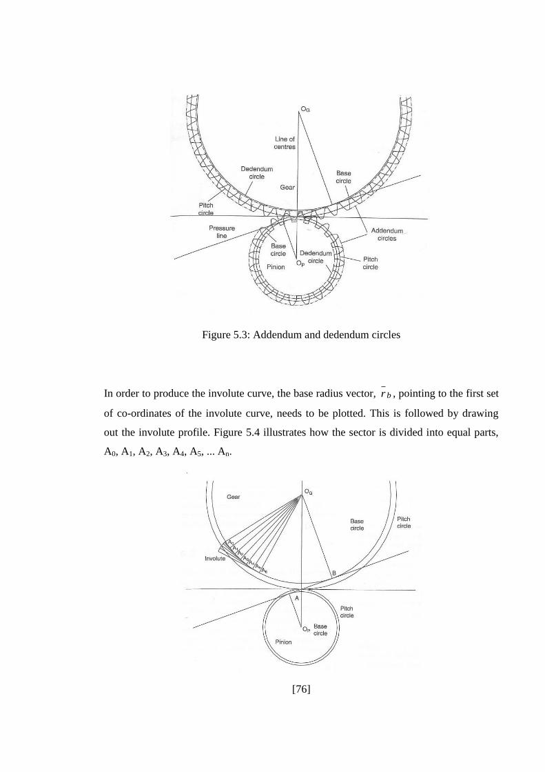
[76]
Figure 5.3: Addendum and dedendum circles
In order to produce the involute curve, the base radius vector, br , pointing to the first set
of co-ordinates of the involute curve, needs to be plotted. This is followed by drawing
out the involute profile. Figure 5.4 illustrates how the sector is divided into equal parts,
A0, A1, A2, A3, A4, A5, ... An.
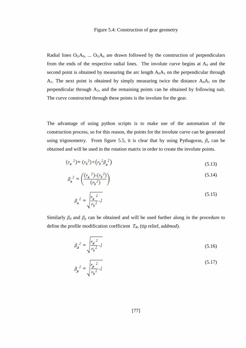
[77]
Figure 5.4: Construction of gear geometry
Radial lines OGA0, ... OGAn are drawn followed by the construction of perpendiculars
from the ends of the respective radial lines. The involute curve begins at A0 and the
second point is obtained by measuring the arc length A0A1 on the perpendicular through
A1. The next point is obtained by simply measuring twice the distance A0A1 on the
perpendicular through A2, and the remaining points can be obtained by following suit.
The curve constructed through these points is the involute for the gear.
The advantage of using python scripts is to make use of the automation of the
construction process, so for this reason, the points for the involute curve can be generated
using trigonometry. From figure 5.5, it is clear that by using Pythagoras, βa can be
obtained and will be used in the rotation matrix in order to create the involute points.
(5.13)
(5.14)
(5.15)
Similarly βd and βp can be obtained and will be used further along in the procedure to
define the profile modification coefficient TR, (tip relief, addmod).
(5.16)
(5.17)
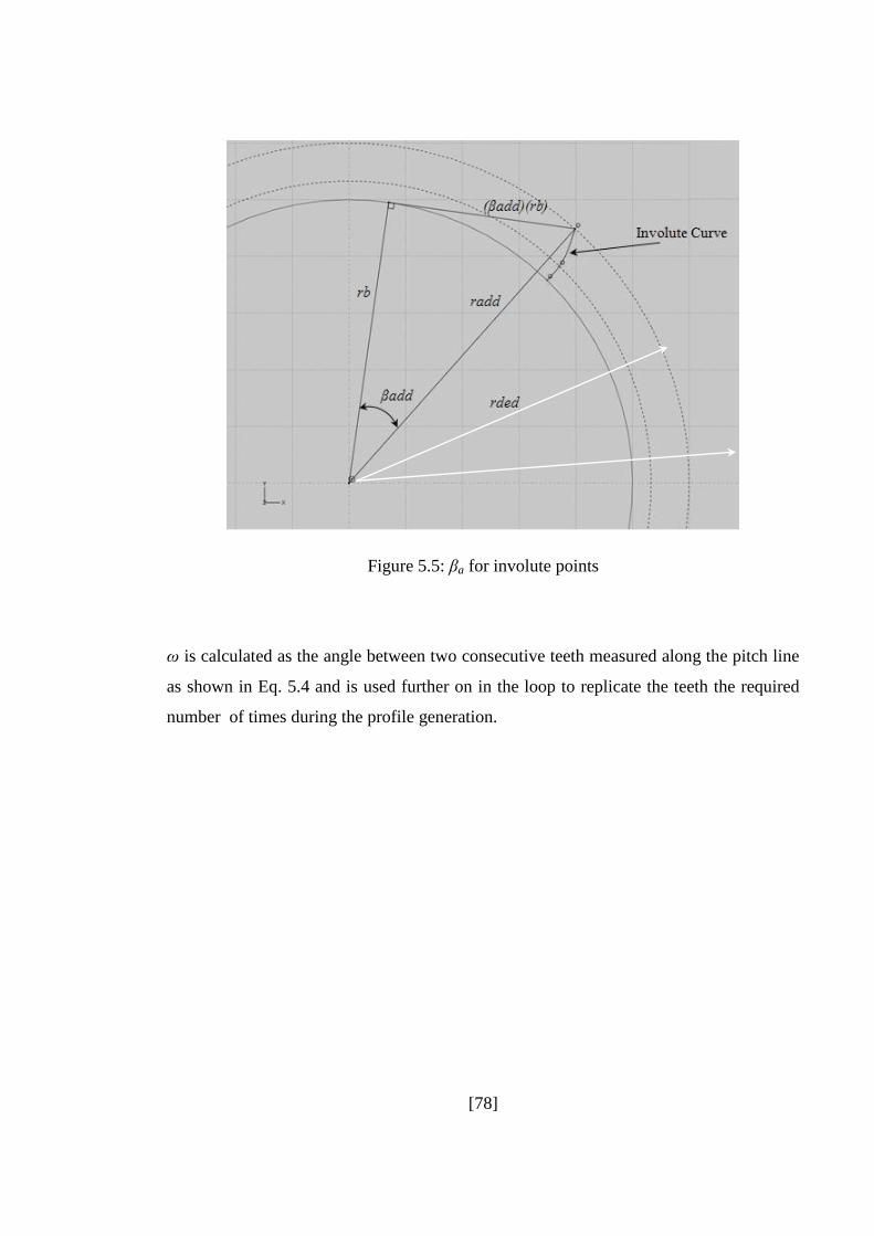
[78]
Figure 5.5: βa for involute points
ω is calculated as the angle between two consecutive teeth measured along the pitch line
as shown in Eq. 5.4 and is used further on in the loop to replicate the teeth the required
number of times during the profile generation.
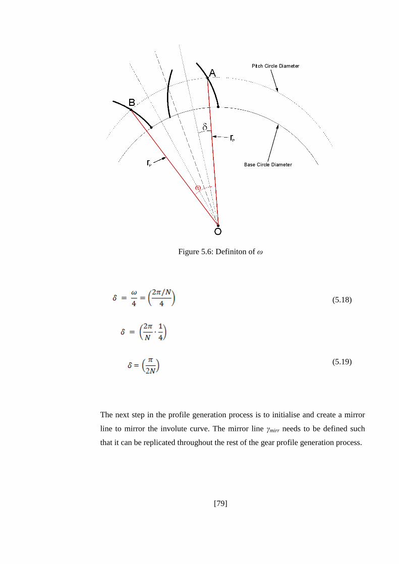
[79]
Figure 5.6: Definiton of ω
(5.18)
(5.19)
The next step in the profile generation process is to initialise and create a mirror
line to mirror the involute curve. The mirror line γmirr needs to be defined such
that it can be replicated throughout the rest of the gear profile generation process.
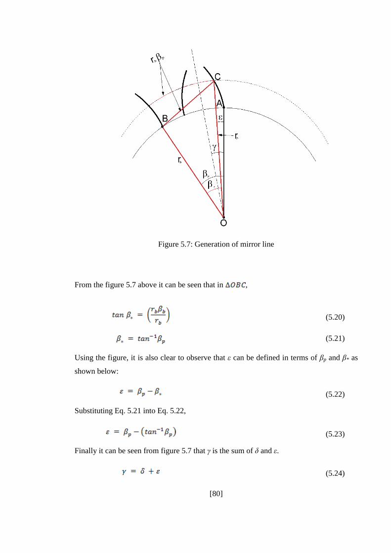
[80]
Figure 5.7: Generation of mirror line
From the figure 5.7 above it can be seen that in ,
(5.20)
(5.21)
Using the figure, it is also clear to observe that ε can be defined in terms of βp and β* as
shown below:
(5.22)
Substituting Eq. 5.21 into Eq. 5.22,
(5.23)
Finally it can be seen from figure 5.7 that γ is the sum of δ and ε.
(5.24)
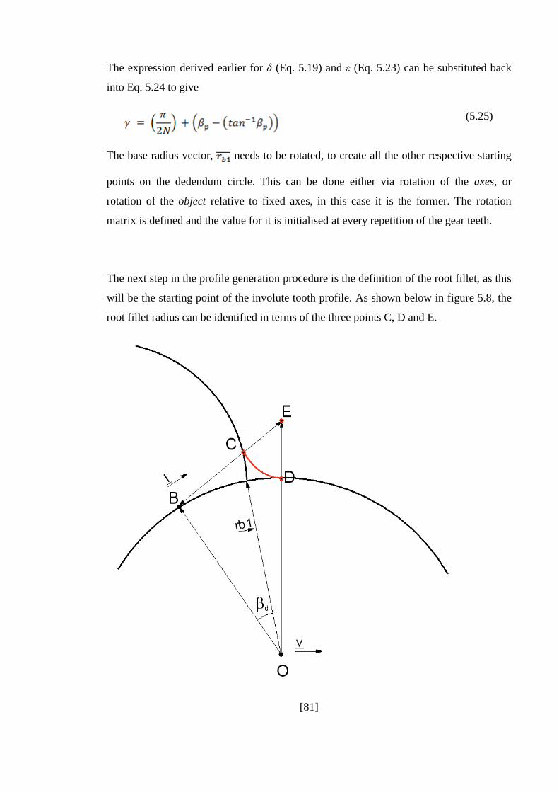
[81]
The expression derived earlier for δ (Eq. 5.19) and ε (Eq. 5.23) can be substituted back
into Eq. 5.24 to give
(5.25)
The base radius vector, needs to be rotated, to create all the other respective starting
points on the dedendum circle. This can be done either via rotation of the axes, or
rotation of the object relative to fixed axes, in this case it is the former. The rotation
matrix is defined and the value for it is initialised at every repetition of the gear teeth.
The next step in the profile generation procedure is the definition of the root fillet, as this
will be the starting point of the involute tooth profile. As shown below in figure 5.8, the
root fillet radius can be identified in terms of the three points C, D and E.
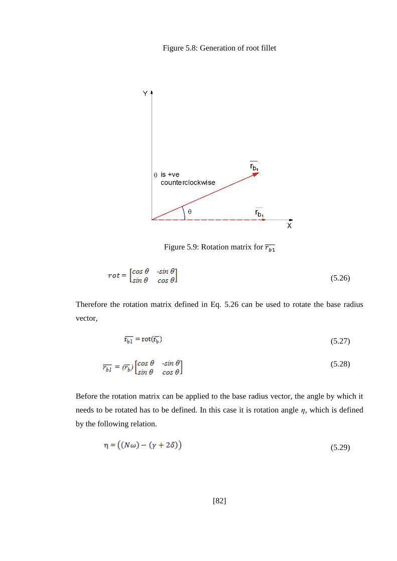
[82]
Figure 5.8: Generation of root fillet
Figure 5.9: Rotation matrix for
(5.26)
Therefore the rotation matrix defined in Eq. 5.26 can be used to rotate the base radius
vector,
(5.27)
(5.28)
Before the rotation matrix can be applied to the base radius vector, the angle by which it
needs to be rotated has to be defined. In this case it is rotation angle η, which is defined
by the following relation.
(5.29)
[83]
The final part of the procedure deals with the definition of the root fillet of the gear teeth
profile. The root fillet needs to be tangential to the dedendum circle and the involute
curve. In fact the root fillet must start at the first point of the involute curve.
5.2 Finite element analysis in Abaqus
The main aim of this section is to provide the reader with all the relevant tools to recreate
the static and dynamic analyses carried out on the gear pair models in this research. The
chapter is arranged in such a way to give a flow of information from the theoretical
basics of finite elements to the practical application of this knowledge in the graphical
user interface in Abaqus.
There are many different approaches made in the research field of gears where finite
elements have been used to simulate their behaviour. Most research work centres on the
finite element formulation of gears in a simplified model such as one with one or two
degrees of freedom [19].
Among other approaches is the use of finite elements to analyse models created using
computer aided design (CAD) programs imported directly into the FE package for
solving [37]. Other researchers have used the matrix laboratory, MATLAB to create
numerical/analytical models of simplified gear systems and combined this with FE
packages to create accurate gear noise prediction tools [40].
This research works to fill the gap in the research field, by using the FE package
strategically to model the gear system accurately with the aid of the automated profile
generation routine developed earlier. The procedure used to fully define the gear systems
is discussed in the following sections.
The Abaqus model of the gear pair designed in this chapter is defined in terms of a model
database, which consists of the part, material properties, analysis steps, loads, boundary
conditions and pre-defined fields, interaction properties and the geometry mesh. In this
section, the various components that make up the model database are briefly introduced
and discussed in terms of setting up the gear pair model.

[84]
[85]
5.3 Analysis steps
Once the geometry of the part is finalised and instanced into the assembly in Abaqus
model database, the analysis procedure needs to be defined. The analysis step can be
summarised as a division of the problem history in time steps, which can have different
analysis procedures, loads and boundary conditions depending on the type of analysis to
be conducted. For each step defined in the analysis, a respective analysis procedure can
be chosen, which then defines the analysis to be run on Abaqus. The only restriction is
that only one analysis procedure can be defined in a step. There are many analysis
procedures that can be defined in Abaqus such as static and dynamic stress/displacement
analysis, heat transfer and thermal stress analysis, electrical analysis, mass diffusion
analysis and acoustic and shock analysis.
5.3.1 General Analysis
In the case of the spur gear pair designed by the automated profile generation procedure,
the Abaqus model databases will be defined in terms of static and dynamic
stress/displacement analysis procedures only. In Chapter 3 it was shown that the results
of TE are generally provided in static cases and used as part of hybrid models, and in
some cases the dynamic TE is calculated in numerical models, hence a direct comparison
between the static and dynamic would provide an insight into the differences between the
two contact problems.
The steps defined in Abaqus are broadly divided into two types based on the response of
the model. General analysis step is used when the response can be either linear or non-
linear and linear perturbation step is used when the response is known to be linear only.
Due to the nature of the response, general analysis can be used in Abaqus/Standard and
Abaqus/Explicit analysis, but linear perturbation is only available on Abaqus/Standard.
5.3.1.1 Material nonlinearity
Material nonlinearity is dependent on the history of the analysis and the materials
response at any time is completely reliant on what happened to it at previous times. The
[86]
solution of the analysis can only be obtained by following the actual loading sequence of
the model.
5.3.1.2 Geometric nonlinearity
Geometric nonlinearity in Abaqus can be ignored or included depending on the type of
analysis being defined. By specifying a small-displacement analysis, the geometric
nonlinearity of the model will be ignored for the respective step of the analysis. This is
usually done by ignoring the nonlinearity in the element calculations and making the
kinematic relationship between them linear. Alternatively, geometric nonlinearity can be
included by specifying a large-displacement analysis, where all the elements are
formulated by using their current nodal coordinates as opposed to their original
coordinates in the small-displacement analysis. Thus the elements sufficiently distort
from their original shape as the deformations of elements in the model increases through
the analysis step.
5.3.1.3 Boundary nonlinearity
Boundary nonlinearity arises from contact formulations which need to be defined in
Abaqus models if contact is a part of the model definition.
In any Abaqus analysis, each step is divided into multiple time increments. The
increments chosen for the analysis step are responsible for controlling the determination
of the finite element solution. The two choices for controlling of the time increments are
automatic time incrementation or user-specified fixed time incrementation. In most cases,
the automatic incrementation is recommended as the solutions to the problem are not
always known and this could allow the Abaqus/Standard to react to any non-linear
response not expected ahead of time.
5.3.2 Linear perturbation analysis step
The linear perturbation analysis step is exclusively used for cases where no non-linear
effects are expected in the analysis and is available only in Abaqus/Standard. The
response in a linear analysis step is the linear perturbation response about the base state.
The base state is the current state of the model at the end of the last general analysis step
[87]
prior to the linear perturbation step. If the first step of an analysis is a perturbation step,
the base state is determined from the initial conditions.
The main restriction on using the linear perturbation analysis for our analysis would be to
do with the contact conditions of the analysis. In a linear perturbation analysis, the
contact conditions cannot change during the analysis. The open or closed status of each
contact constraint remains as it is in the initial or base state. All points in contact (i.e.,
with a “closed” status) are assumed to be sticking if friction is present, except the contact
nodes for which a velocity differential is imposed by the motion of the reference frame or
the transport velocity. At those nodes, slipping conditions are assumed regardless of the
friction coefficient.
5.3.3 Direct linear equation solver
The linear equation solution is used in both linear and nonlinear analyses in Abaqus. In a
nonlinear analysis, Abaqus/Standard uses the Newton method or a variant of it, such as
the Riks method, within which it is necessary to solve a set of linear equations at each
iteration. The direct linear equation solver finds the exact solution to this system of linear
equations up to the allowable machine precision (2E-16). The direct linear equation
solver in Abaqus/Standard uses a sparse, direct, Gauss elimination method.
5.3.4 Iterative linear equation solver
In Abaqus/Standard, the iterative linear equation solver can be used only for linear and
nonlinear static and quasi-static procedures, with a symmetric stiffness matrix and a
single load case in the analysis. The iterative linear solver is mainly based on the domain
decomposition method [80] which deals with the methods used to obtain an approximate
solution of linear or nonlinear systems that use discretization of partial differential
equations.
The iterative linear equation solver is mostly used for very large, well-conditioned
models with nearer to million degrees of freedom. In all other cases the direct linear
equation solver should be used.
[88]
5.3.5 Dynamic analysis
Abaqus offers us the choice of linear or nonlinear dynamic analysis, but in the case of
this work the dynamic analysis will be carried out on Abaqus including inertial effects
and the dynamic nonlinear system response to the input torque at the driving gear.
In the case of nonlinear analysis, there is a choice of between modal and direct
integration methods. In the case of slightly nonlinear systems, the modal method can be
used and usually performed by using the eigen-modes of the system as a basis for
calculating the response. The mode based procedure is computationally less expensive
than other methods, and is relatively simple to use. For strongly nonlinear problems, the
dynamic response of the system is obtained by the direct integration method applied to
all the degrees of freedom of the finite element model.
The main choice of operator to be used to analyse our gear pair system lies in the way the
model will be defined. In our model, the driver and driven gears are given full material
properties along with density and material damping. The loading and constraints of the
systems are identical to the static nonlinear case and the only difference being the
analysis type changing from static to dynamic. The integration operators used in dynamic
analysis in Abaqus are generally divided as implicit or explicit.
5.3.5.1 Explicit analysis
The explicit operations used in Abaqus/Explicit need to have values for time t given for
the analysis, and hence obtain values for dynamic quantities at based on the
values given. The most commonly used explicit operator for stress analysis applications
is the central difference operator, which is only conditionally stable and is influenced by
the size of the smallest element in the model. This is because the stability limit of the
central difference operator is approximately the time it takes an elastic wave to cross the
smallest element dimension in the model.
5.3.5.2 Implicit analysis
Utilising the implicit scheme removes this limitation on time step size by solving for any
dynamic quantities at time based on the given time t, but also for the same
[89]
quantities at time . As they are implicit operations, the nonlinear equations now
need to be solved. In structural problems implicit integration schemes usually give
acceptable solutions with time steps typically one or two orders of magnitude larger than
the stability limit of simple explicit schemes, but the response prediction will deteriorate
as the time step size , increases relative to the period, T, of typical modes of response.
When considering the maximum time step size, there are three main points that should be
considered: the rate of variation of the applied loading, the complexity of the nonlinear
damping and stiffness properties, and the typical period of vibration of the structure.
All these factors contribute to the definition of the implicit dynamic analysis step that has
to be used in our gear pair dynamic nonlinear analysis. Initially attempts were also made
to analyse the gear pair system using explicit dynamics, but these were not successful,
and will be discussed briefly further on in Chapter 7.
The main attributes that need to be defined in the step module for the implicit analysis
are the total time t,
5.3.5.3 Implicit versus explicit analysis
The direct-integration dynamic procedure provided in Abaqus/Standard uses the implicit
Hilber-Hughes-Taylor operator for integration of the equations of motion, while
Abaqus/Explicit uses the central-difference operator. In an implicit dynamic analysis the
integration operator matrix must be inverted and a set of nonlinear equilibrium equations
must be solved at each time increment. In an explicit dynamic analysis displacements and
velocities are calculated in terms of quantities that are known at the beginning of an
increment; therefore, the global mass and stiffness matrices need not be formed and
inverted, which means that each increment is relatively inexpensive compared to the
increments in an implicit integration scheme. The size of the time increment in an
explicit dynamic analysis is limited, however, because the central-difference operator is
only conditionally stable; whereas the Hilber-Hughes-Taylor operator is unconditionally
stable and, thus, there is no such limit on the size of the time increment that can be used
for most analyses in Abaqus/Standard (accuracy governs the time increment in
Abaqus/Standard).
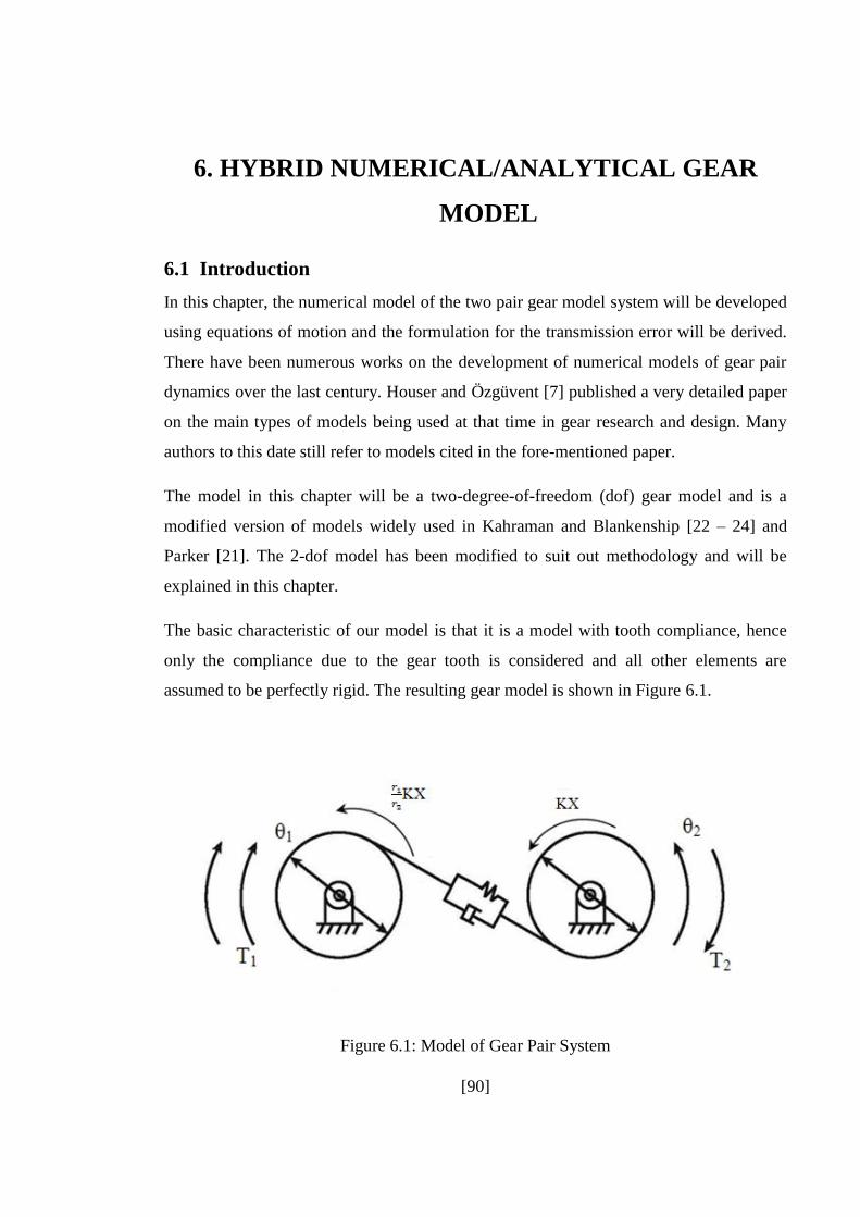
[90]
6. HYBRID NUMERICAL/ANALYTICAL GEAR
MODEL
6.1 Introduction
In this chapter, the numerical model of the two pair gear model system will be developed
using equations of motion and the formulation for the transmission error will be derived.
There have been numerous works on the development of numerical models of gear pair
dynamics over the last century. Houser and Özgüvent [7] published a very detailed paper
on the main types of models being used at that time in gear research and design. Many
authors to this date still refer to models cited in the fore-mentioned paper.
The model in this chapter will be a two-degree-of-freedom (dof) gear model and is a
modified version of models widely used in Kahraman and Blankenship [22 – 24] and
Parker [21]. The 2-dof model has been modified to suit out methodology and will be
explained in this chapter.
The basic characteristic of our model is that it is a model with tooth compliance, hence
only the compliance due to the gear tooth is considered and all other elements are
assumed to be perfectly rigid. The resulting gear model is shown in Figure 6.1.
Figure 6.1: Model of Gear Pair System
[91]
In our 2-dof model, the gear system is idealised as a pair of inertias coupled with a spring
which allows relative motion. Using the 2-dof model, one can study the rotational
vibrations of the gear systems as a result of an angular velocity input and the
transmission error excitation is simulated by the displacement excitation of the teeth in
mesh.
6.2 Gear model system
First the simpler model with no clearance between the gear pairs and no damping will be
considered and the respective equations of motion will be derived. Then the backlash will
be added along with the damping coefficient in order to define the final model and the
equations of motion will be finally derived.
Consider a gear system with two gears, the driver and driven, each having radii r1 and r2,
respectively. The driver has an input angular velocity of θ1 applied onto it and this causes
the driven gear to rotate with an angular velocity of θ2.
In an idealised system with no transmission error present between the gears, the angular
velocity applied to the driver will obviously make the driven gear move with the angular
velocity of the driving gear multiplied by the ratio . Therefore, when there is no
transmission error,
As stated previously in this Thesis, transmission error (TE) is the deviation in position of
the driven gear, relative to where it should be if both gears were geometrically perfect
and have no deformation. This is highly idealised and even if the gears were
geometrically perfect, avoiding deformation on contact is “almost” impossible. In this
model the transmission error will be indicated as X, is measured in radian and defined as:
where θ1 and θ2 are assumed positive if clockwise in the case of the former and anti-
clockwise for the latter.
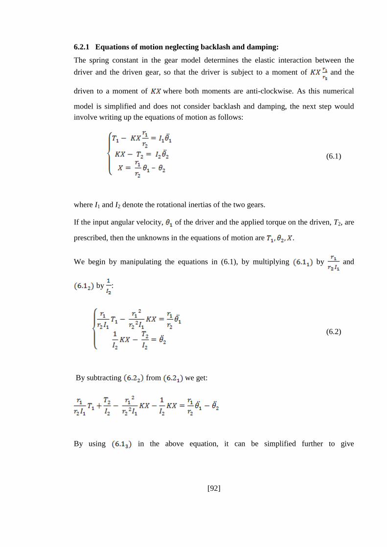
[92]
6.2.1 Equations of motion neglecting backlash and damping:
The spring constant in the gear model determines the elastic interaction between the
driver and the driven gear, so that the driver is subject to a moment of and the
driven to a moment of where both moments are anti-clockwise. As this numerical
model is simplified and does not consider backlash and damping, the next step would
involve writing up the equations of motion as follows:
(6.1)
where I1 and I2 denote the rotational inertias of the two gears.
If the input angular velocity, of the driver and the applied torque on the driven, T2, are
prescribed, then the unknowns in the equations of motion are .
We begin by manipulating the equations in (6.1), by multiplying by and
by :
(6.2)
By subtracting from we get:
By using in the above equation, it can be simplified further to give

[93]
(6.3)
Using the input angular velocity of the driver , the equation can be manipulated
to make the subject of interest, giving us:
(6.4)
Substituting (6.4) into (6.3) gives:
Where some terms cancel out so that one has:
Multiplying the above equation throughout by :
(6.5)
This is the equation of motion for the 2 degree of freedom gear pair system
6.2.2 Equations of motion with backlash and damping:
Let us assume that is the angular rotation of the driven gear which puts the gears in
contact starting from the initial position. Hence, if the driven gear is rotated, contact
would be reached for or as shown in Figure 6.2.

[94]
Figure 6.2: Backlash for Gear Pair System
Therefore, if the driver gear was rotated instead of the driven, contact would be reached
for the angular velocity, or . Hence it can be summarised that the
rotational stiffness only acts on the teeth when . This is because the backlash
coefficient is mirrored about the mirror line of the teeth is thus present on both sides of
the teeth for the driver and driven gears.
Therefore the gear pair system can be modelled as shown below in Figure 6.3:
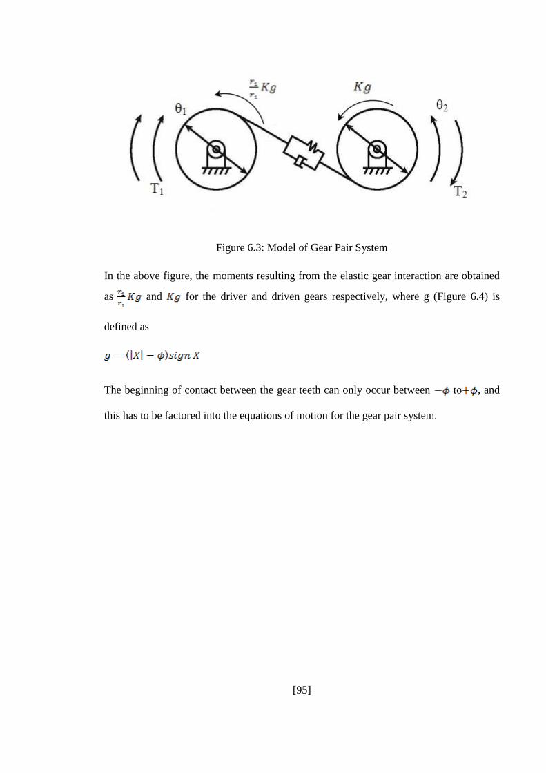
[95]
Figure 6.3: Model of Gear Pair System
In the above figure, the moments resulting from the elastic gear interaction are obtained
as and for the driver and driven gears respectively, where g (Figure 6.4) is
defined as
The beginning of contact between the gear teeth can only occur between to , and
this has to be factored into the equations of motion for the gear pair system.
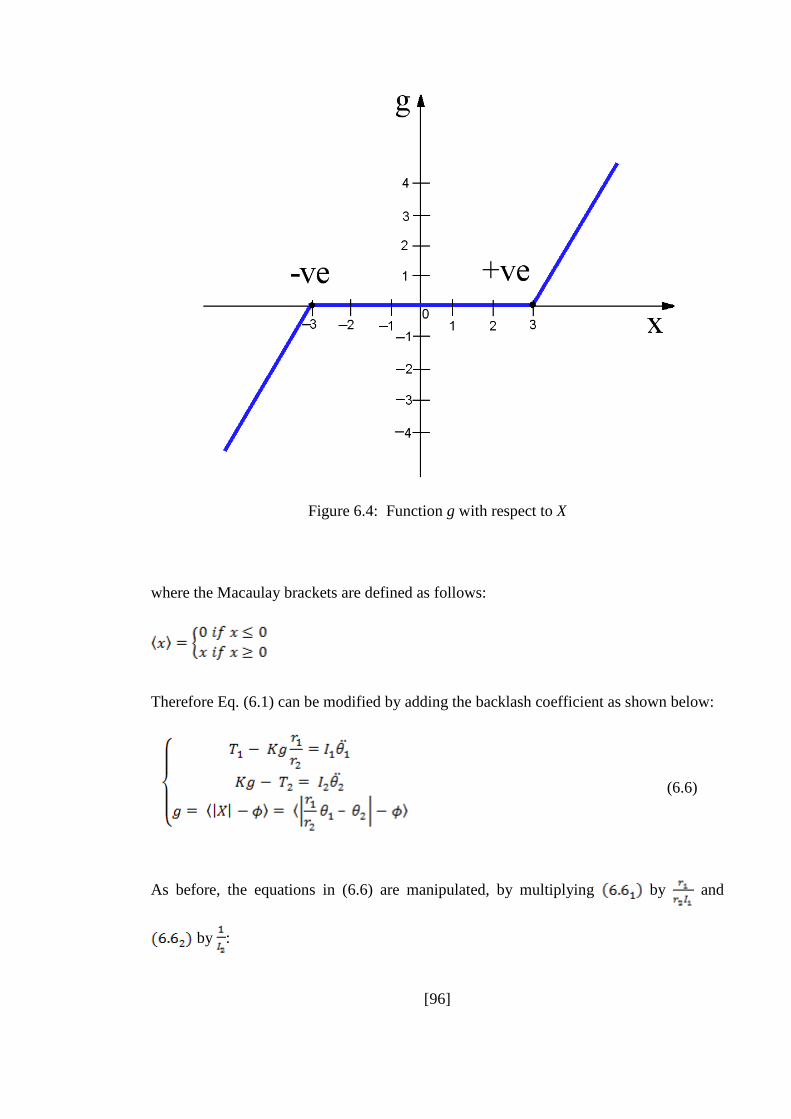
[96]
Figure 6.4: Function g with respect to X
where the Macaulay brackets are defined as follows:
Therefore Eq. (6.1) can be modified by adding the backlash coefficient as shown below:
(6.6)
As before, the equations in (6.6) are manipulated, by multiplying by and
by :
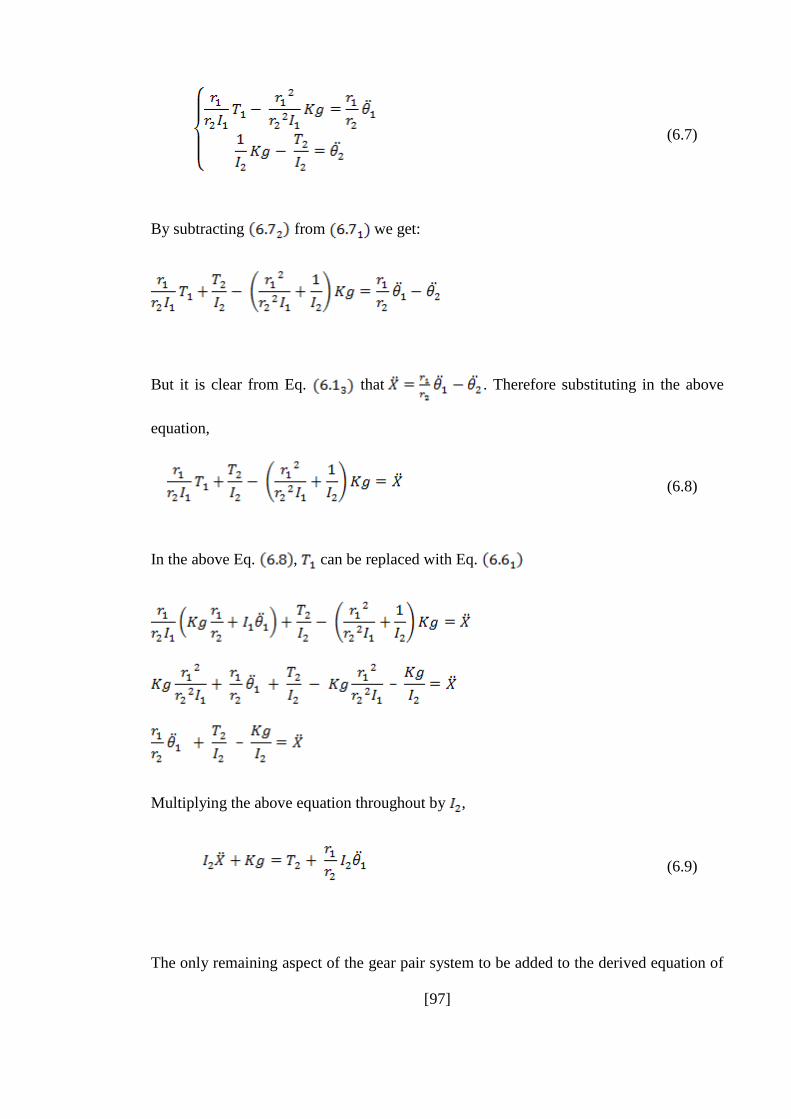
[97]
(6.7)
By subtracting from we get:
But it is clear from Eq. that . Therefore substituting in the above
equation,
(6.8)
In the above Eq. , can be replaced with Eq.
Multiplying the above equation throughout by ,
(6.9)
The only remaining aspect of the gear pair system to be added to the derived equation of
[98]
motion is the damping term, . Damping is an important aspect in the behaviour of the
gear pair model as it controls the time taken for the system to reach a steady state
condition. The sources of damping in the system are mainly the friction within the
bearing and the internal material damping. While the latter is typically well represented
with a linear viscous term, an accurate description of frictional damping would require a
more complex, non-linear formulation. For the purpose of this research the linear viscous
damping term is considered an adequate approximation. The final equation of motion
for the 2 dof gear pair model can finally be derived as:
(6.10)
where,
6.2.3 Prescribed velocity, applied torque, initial conditions and stiffness K
The angular velocity of the driving gear is assumed to be constant, whereby the term
containing the angular acceleration is null. The applied torque on the driven gear is also
assumed constant and equal to T2. As for the initial conditions, we will always consider
, resulting in . For the initial velocity we will consider two values and
corresponding to the case of ideal no transmission error, whereby:
resulting in .

[99]
The rotational stiffness constant K has to be defined in order to solve the equation of
motion. Considering the 2dof gear pair model as a static model, where there are no
inertia forces to consider, Eq. (6.10) can be simplified as
Therefore, the stiffness is found by conducting a quasi-static finite-element analysis and
by determining the static transmission error, which accounting for the backlash is exactly
equal to g.
6.2.4 Time integration of the equation of motion:
The following section of the chapter will deal with the time integration of the derived
equation of motion for the 2 dof gear pair model. The time interval is subdivided into a
number of increments. Let us consider the time intervals and
assume that are known, leaving to be calculated. Thus
Eq. can be rewritten as
(6.11)
Since the initial conditions , the first two values and are
also taken to be equal to zero. Hence the algorithm starts at . The time integration
of the equation of motion can be carried out with the use of the finite difference method.
The finite difference method is a discrete analogue of the derivative, where the finite
forward difference of a function is defined as
and the finite backwards difference is defined as
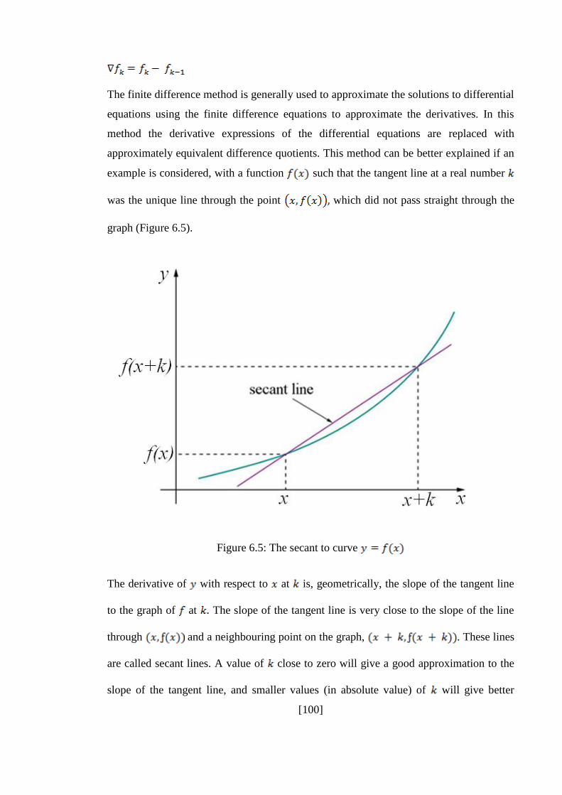
[100]
The finite difference method is generally used to approximate the solutions to differential
equations using the finite difference equations to approximate the derivatives. In this
method the derivative expressions of the differential equations are replaced with
approximately equivalent difference quotients. This method can be better explained if an
example is considered, with a function such that the tangent line at a real number
was the unique line through the point which did not pass straight through the
graph (Figure 6.5).
Figure 6.5: The secant to curve
The derivative of with respect to at is, geometrically, the slope of the tangent line
to the graph of at The slope of the tangent line is very close to the slope of the line
through and a neighbouring point on the graph, . These lines
are called secant lines. A value of close to zero will give a good approximation to the
slope of the tangent line, and smaller values (in absolute value) of will give better

[101]
approximations. The slope of the secant line is the difference between the values of
these points divided by the difference between the values such that,
Using the above principle in Eq. for the case of the 2 dof gear pair model, is
represented by,
(6.12)
The additional intermediate times can then be introduced as follows
Similarly, defining
(6.13)
The above equations can be used to define the second time derivative :

[102]
This can be simplified by substituting Eq. and Eq. , giving:
Let and ,
Substituting and back into the equation,
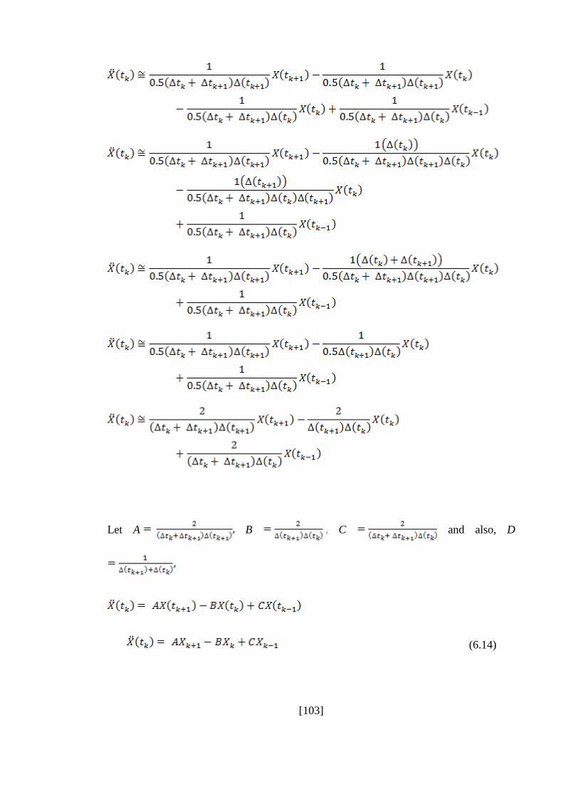
[103]
Let A B C and also, D
(6.14)
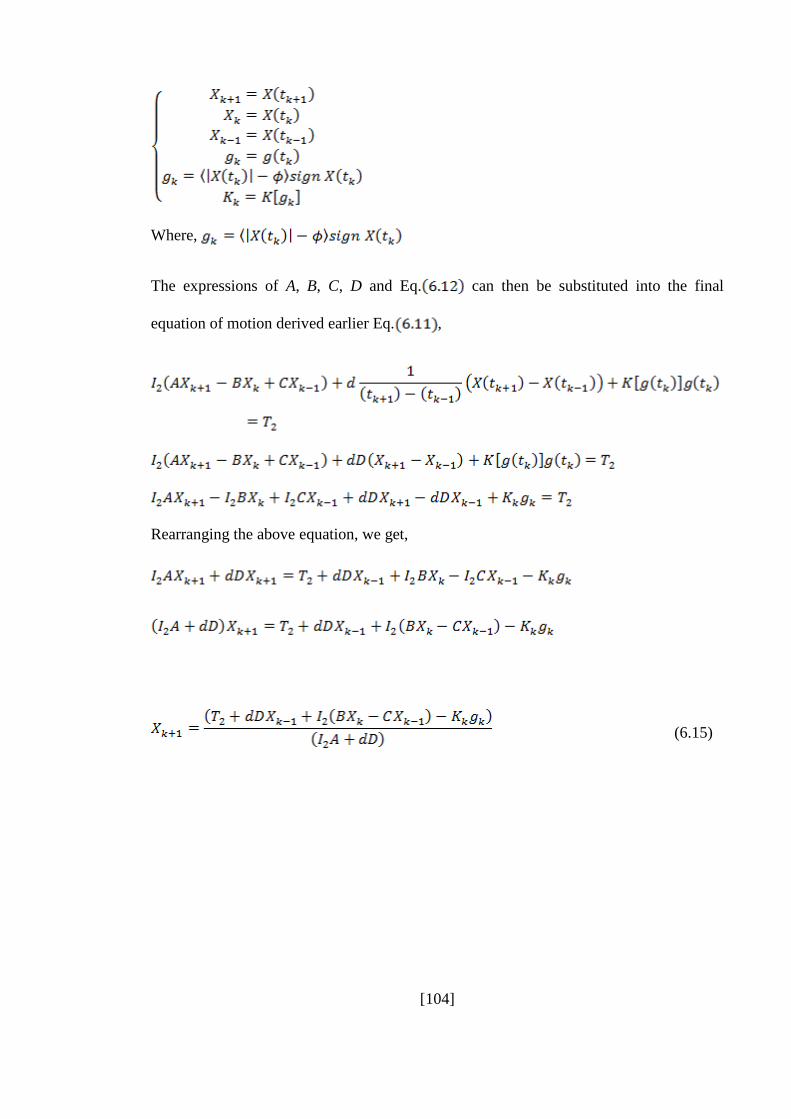
[104]
Where,
The expressions of A, B, C, D and Eq. can then be substituted into the final
equation of motion derived earlier Eq. ,
Rearranging the above equation, we get,
(6.15)

[105]
7. STATIC VERSUS DYNAMIC TRANSMISSION
ERROR
In Chapters 1 and 3, it has been observed that most researchers who worked on the
modelling of transmission error are split into two distinct groups: those who perform
static analyses, leading to the computation of the static transmission error (STE) and
those who conduct dynamic analyses, leading to the determination of the dynamic
transmission error (DTE).
A careful review of the literature revealed that no published work addressed the
following fundamental question: What is the difference in the results using either
approach?
The same review of the literature revealed that all the research work addressing the
determination of the DTE is based either on analytical methods, see for instance [59, 64,
69], or on numerical methods in which the stiffness of the system is accurately derived
using finite-element analysis, but the dynamics of the system is studied using simplified
(typically one- or two-degree-of-freedom) models [50, 66, 67]. The latter approach has
been indicated in this work as the ‘hybrid numerical/analytical’ approach and already
described in Chapter 6.
Therefore, the following second fundamental question arose in this research work: What
is the level of approximation entailed by these simplifications?
To answer this second question it was thought that a full non-linear dynamic analysis of a
pair of spur gear could be conducted, which leads to the further issue of understanding
the level of accuracy entailed by such an analysis and how that is related to the many
parameters which need to be specified, such as the parameters for the contact algorithm,
the mesh refinement, the convergence tolerance, etc …
This chapter aims to answer these fundamental questions and represents the most original
contribution of the dissertation.
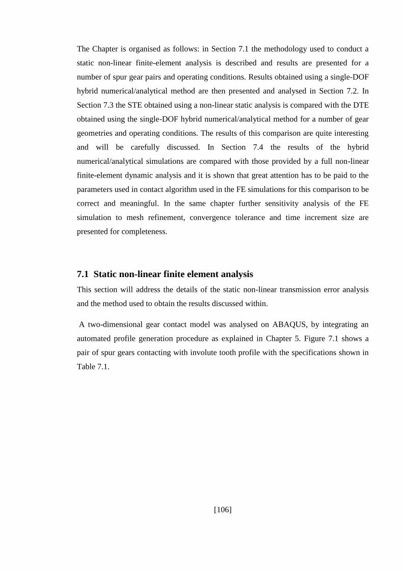
[106]
The Chapter is organised as follows: in Section 7.1 the methodology used to conduct a
static non-linear finite-element analysis is described and results are presented for a
number of spur gear pairs and operating conditions. Results obtained using a single-DOF
hybrid numerical/analytical method are then presented and analysed in Section 7.2. In
Section 7.3 the STE obtained using a non-linear static analysis is compared with the DTE
obtained using the single-DOF hybrid numerical/analytical method for a number of gear
geometries and operating conditions. The results of this comparison are quite interesting
and will be carefully discussed. In Section 7.4 the results of the hybrid
numerical/analytical simulations are compared with those provided by a full non-linear
finite-element dynamic analysis and it is shown that great attention has to be paid to the
parameters used in contact algorithm used in the FE simulations for this comparison to be
correct and meaningful. In the same chapter further sensitivity analysis of the FE
simulation to mesh refinement, convergence tolerance and time increment size are
presented for completeness.
7.1 Static non-linear finite element analysis
This section will address the details of the static non-linear transmission error analysis
and the method used to obtain the results discussed within.
A two-dimensional gear contact model was analysed on ABAQUS, by integrating an
automated profile generation procedure as explained in Chapter 5. Figure 7.1 shows a
pair of spur gears contacting with involute tooth profile with the specifications shown in
Table 7.1.
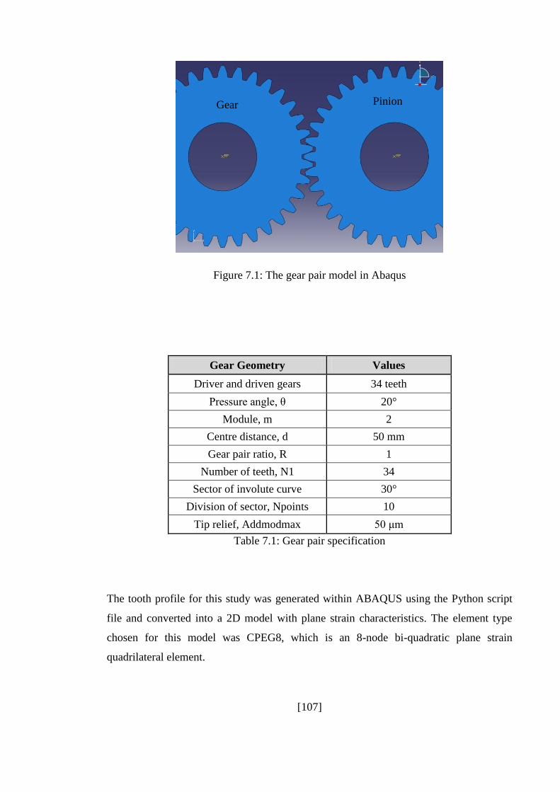
[107]
Figure 7.1: The gear pair model in Abaqus
Gear Geometry Values
Driver and driven gears 34 teeth
Pressure angle, θ 20°
Module, m 2
Centre distance, d 50 mm
Gear pair ratio, R 1
Number of teeth, N1 34
Sector of involute curve 30°
Division of sector, Npoints 10
Tip relief, Addmodmax 50 μm
Table 7.1: Gear pair specification
The tooth profile for this study was generated within ABAQUS using the Python script
file and converted into a 2D model with plane strain characteristics. The element type
chosen for this model was CPEG8, which is an 8-node bi-quadratic plane strain
quadrilateral element.
Gear
(Driver)
Pinion
(Driven)
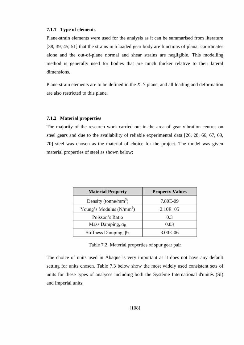
[108]
7.1.1 Type of elements
Plane-strain elements were used for the analysis as it can be summarised from literature
[38, 39, 45, 51] that the strains in a loaded gear body are functions of planar coordinates
alone and the out-of-plane normal and shear strains are negligible. This modelling
method is generally used for bodies that are much thicker relative to their lateral
dimensions.
Plane-strain elements are to be defined in the X–Y plane, and all loading and deformation
are also restricted to this plane.
7.1.2 Material properties
The majority of the research work carried out in the area of gear vibration centres on
steel gears and due to the availability of reliable experimental data [26, 28, 66, 67, 69,
70] steel was chosen as the material of choice for the project. The model was given
material properties of steel as shown below:
Material Property Property Values
Density (tonne/mm3) 7.80E-09
Young’s Modulus (N/mm2) 2.10E+05
Poisson’s Ratio 0.3
Mass Damping, αR 0.03
Stiffness Damping, βR 3.00E-06
Table 7.2: Material properties of spur gear pair
The choice of units used in Abaqus is very important as it does not have any default
setting for units chosen. Table 7.3 below show the most widely used consistent sets of
units for these types of analyses including both the Système International d'unités (SI)
and Imperial units.

[109]
Quantity SI SI (mm) SI
US Unit
(ft)
US Unit
(inch)
Length m mm m ft inch
Force N N kN lbf lbf
Mass kg tonne (103kg) tonne slug ilbfs2/in
Time s s s s s
Stress N/m2 (Pa) N/mm
2 (MPa) kPa lbf/ft
2 lbf/in
2 (psi)
Energy J mJ (10-3J) KJ ftlbf inlbf
Density kg/m3 tonne/mm
3 tonne/m
3 slug/ft
3 lbfs
2/in
4
Table 7.3: consistent sets of units
7.1.3 Analysis Type
As this is a static non-linear analysis, the analysis procedure used in the analysis step
must be set to “static stress/displacement analysis”. In this type of analysis, the inertial
effects of the parts are neglected along with any time dependent material effects such as
creep, crack propagation and visco-elastic effect. The static analysis can be of a linear or
non-linear type and this essentially influences the specification of appropriate boundary
conditions for the analysis.
In the case of the spur gear pair being modelled in our work, non-linear effects can be
expected in the form of large-displacement effects and contact nonlinearities which must
be accounted for. As geometrically nonlinear behaviour is present in our analysis, the
large-displacement formulation will be used in the model definition.
Following the successful definition of the load steps for the gear pair models, the
interactions between the teeth need to be specified. Ideally in the simulation a minimum
of 2 full contact teeth interactions need to be modelled. In this study three complete gear
pair interactions have been defined and analysed. Friction has been neglected whilst
specifying the properties of the teeth interaction.
7.1.4 Interaction property
One of the significant properties to be considered in defining the teeth interactions is the
type of contact between the interfacing surfaces, which in the simulation is set to finite

[110]
sliding, with surface to surface contact. The master and slave surfaces that need to be
picked to complete the interaction properties depend on the driver and driven gears
respectively. Once the interaction properties for the gear pair models are defined, then
these properties are simply propagated to the other steps of the analysis. Further research
into how the contact algorithm influences the results of the analysis has been carried out
and reported in Section 7.4.
In the static non-linear simulation, a load of 5000Nmm is applied to the driven gear as a
ramped function in the contact step and is applied instantaneously over the rotation step
as defined in Chapter 5. The gear rotation angle is set larger than the gear base pitch
angle to achieve a complete history of more than one tooth mating. Fig. 7.2 shows a
sequence of contact stress distribution plots of two teeth in contact as they rotate
clockwise through the mesh. It can be seen that the highest von Mises stress is located
underneath the contact surface, which is as reported in traditional contact theory [31, 45,
51, 59] and that the contact ratio of the gear pairs is more than 1.0.
Max.V.Mises
Stress 1
2
1
2
1
2
1
2
1
2
1
2
1
2
1
2
3
[111]
Figure 7.2: Static non-linear gear contact maximum stress
7.1.5 The static transmission error
The transmission error is calculated by obtaining the rotations of the central reference
nodes in both the driver and driven gear pairs (Appendix 5) and input into the formula
given in Eq. (3.1) in Chapter 3.
(3.1)
As explained in Chapter 3, there is inconsistency in the literature in the way transmission
error is reported. The three main ways of reporting TE are divided on the units that are
used to represent the error or “displacement”. One method uses angular rotation with
units of radians, another one uses angular displacements with units of arc sec and more
recently the general trend has been to convert the transmission error into linear
displacement at either the base radius or pitch radius of the output gear with units of m
or in.
Using the justification from Chapter 3, for this thesis we shall be using the pitch circle
radius as it ties in with the standard way of defining pitch errors between teeth. From
here on in when referring to the transmission error, the units of m (microns) will be
used. Finally specifying transmission error as a linear displacement is convenient because
all gears of a given manufacturing quality, regardless of tooth size and module, have
about the same size of transmission errors, thus making comparison relatively easy
1
2
1
2
3
1
2
1
2
3

[112]
(typically around 5 m) [51]. The transmission error is generally accepted as being
independent of the gear size, hence making the gear diameter an unimportant variable
that can be adjusted if needed. To give the reader an idea for the range of TE values to
expect from a gear pair, it can be summarised from literature [8, 38, 45, 51] that values of
the peak-to-peak transmission error (PPTE) higher than 10 are considered typical of
rough and very poorly designed gears.
For large slow-speed gears, a PPTE of 20 would normally be expected and is often
seen on the sort of machinery where gear noise is not really a problem. At the other end
of the spectrum, for a high precision gear pair, a PPTE of 1 is extremely good and in
reality is rarely achieved [51]. Medium and small sized industrial gears will generally be
very satisfactory with less than 3 to 4 at 1/tooth p-p and this level should be achieved
with quality gears.
Figure 7.3: Static transmission error from a typical static non-linear analysis.
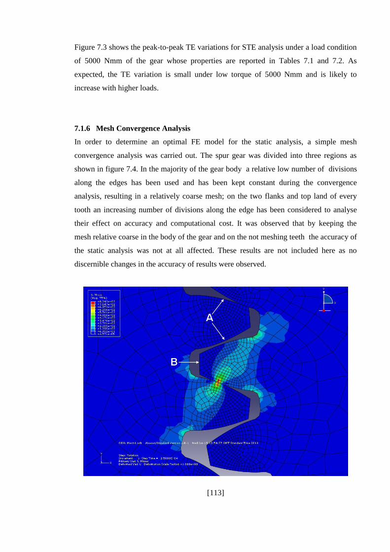
[113]
Figure 7.3 shows the peak-to-peak TE variations for STE analysis under a load condition
of 5000 Nmm of the gear whose properties are reported in Tables 7.1 and 7.2. As
expected, the TE variation is small under low torque of 5000 Nmm and is likely to
increase with higher loads.
7.1.6 Mesh Convergence Analysis
In order to determine an optimal FE model for the static analysis, a simple mesh
convergence analysis was carried out. The spur gear was divided into three regions as
shown in figure 7.4. In the majority of the gear body a relative low number of divisions
along the edges has been used and has been kept constant during the convergence
analysis, resulting in a relatively coarse mesh; on the two flanks and top land of every
tooth an increasing number of divisions along the edge has been considered to analyse
their effect on accuracy and computational cost. It was observed that by keeping the
mesh relative coarse in the body of the gear and on the not meshing teeth the accuracy of
the static analysis was not at all affected. These results are not included here as no
discernible changes in the accuracy of results were observed.
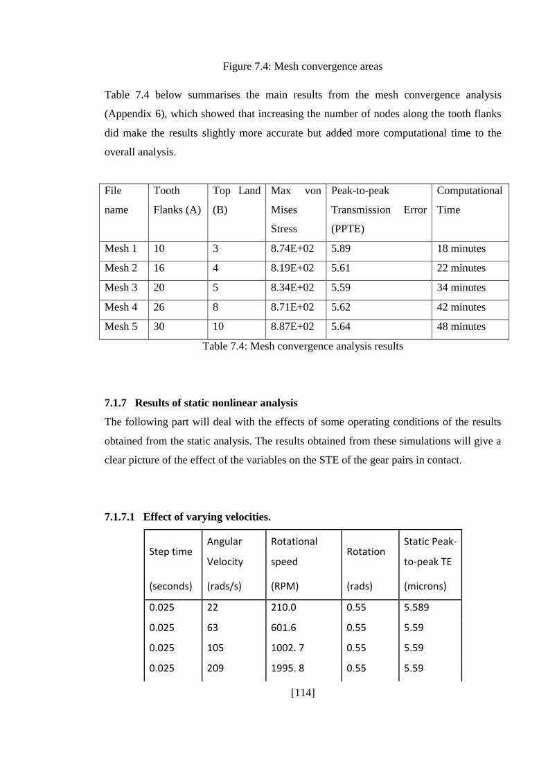
[114]
Figure 7.4: Mesh convergence areas
Table 7.4 below summarises the main results from the mesh convergence analysis
(Appendix 6), which showed that increasing the number of nodes along the tooth flanks
did make the results slightly more accurate but added more computational time to the
overall analysis.
File
name
Tooth
Flanks (A)
Top Land
(B)
Max von
Mises
Stress
Peak-to-peak
Transmission Error
(PPTE)
Computational
Time
Mesh 1 10 3 8.74E+02 5.89 18 minutes
Mesh 2 16 4 8.19E+02 5.61 22 minutes
Mesh 3 20 5 8.34E+02 5.59 34 minutes
Mesh 4 26 8 8.71E+02 5.62 42 minutes
Mesh 5 30 10 8.87E+02 5.64 48 minutes
Table 7.4: Mesh convergence analysis results
7.1.7 Results of static nonlinear analysis
The following part will deal with the effects of some operating conditions of the results
obtained from the static analysis. The results obtained from these simulations will give a
clear picture of the effect of the variables on the STE of the gear pairs in contact.
7.1.7.1 Effect of varying velocities.
Step time Angular
Velocity
Rotational
speed Rotation
Static Peak-
to-peak TE
(seconds) (rads/s) (RPM) (rads) (microns)
0.025 22 210.0 0.55 5.589
0.025 63 601.6 0.55 5.59
0.025 105 1002. 7 0.55 5.59
0.025 209 1995. 8 0.55 5.59

[115]
0.025 419 4001.1 0.55 5.59
Table 7.5: Results from velocity analysis
The transmission error plots below show that there is no variation in the transmission
error plots for the various velocities applied to the gear pair model in the static non-linear
analysis (Figure 7.5). Although this might seem unrealistic when considering real world
principles, one has to take into account the nature of the analysis being carried out. In the
static analysis there are no inertial effects, and the mass property of the model does not
play any role. Therefore, the values for the peak-to-peak STE should all be of the same
value, although there are slight differences which have been rounded up as these are due
to irregularities in the Abaqus contact formulation.
Figure 7.5: STE for varying velocties
This graph illustrates the said point above as the STE curves are virtually on top of each
other and this is to be expected of a static analysis. Hence this serves as an initial
validation of our approach.

[116]
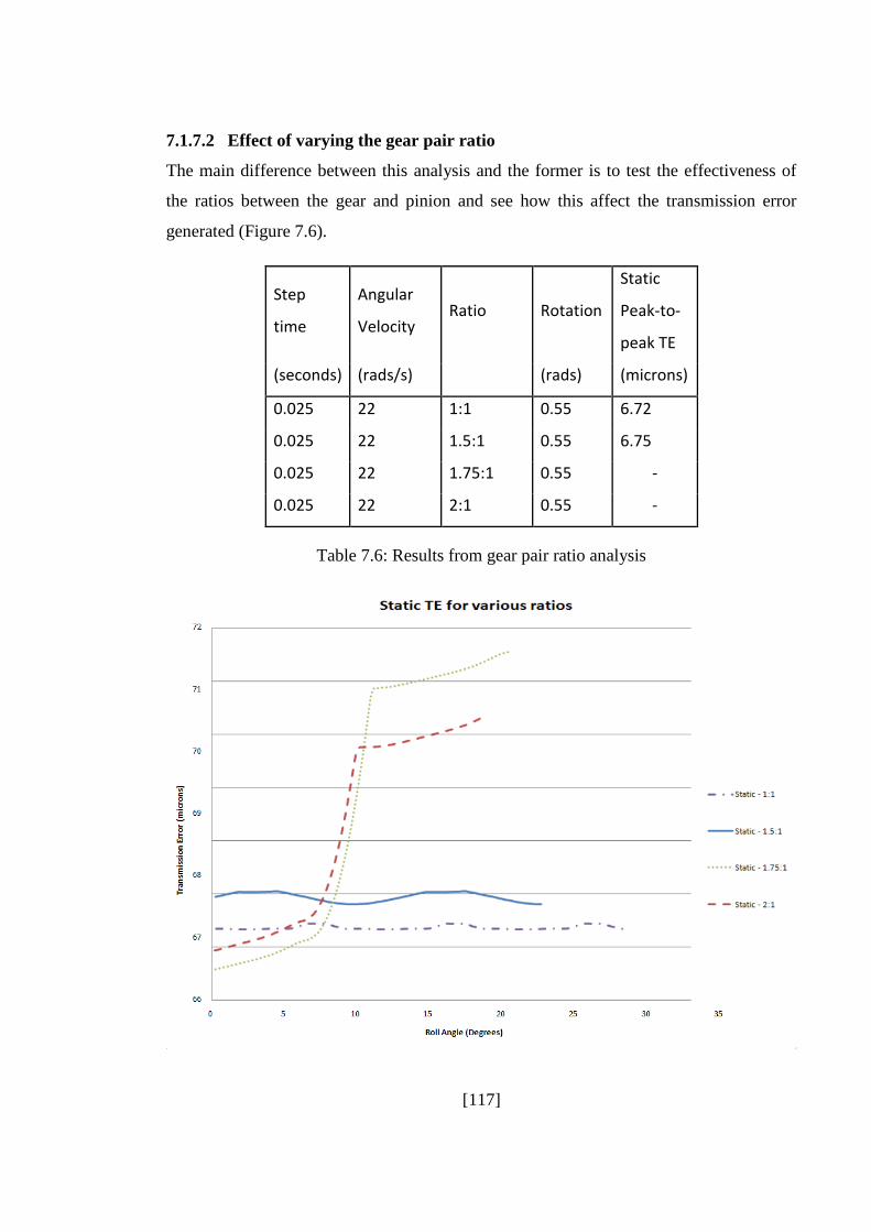
[117]
7.1.7.2 Effect of varying the gear pair ratio
The main difference between this analysis and the former is to test the effectiveness of
the ratios between the gear and pinion and see how this affect the transmission error
generated (Figure 7.6).
Step
time
Angular
Velocity Ratio Rotation
Static
Peak-to-
peak TE
(seconds) (rads/s) (rads) (microns)
0.025 22 1:1 0.55 6.72
0.025 22 1.5:1 0.55 6.75
0.025 22 1.75:1 0.55 -
0.025 22 2:1 0.55 -
Table 7.6: Results from gear pair ratio analysis
[118]
Figure 7.6: STE for different ratios
The gear ratios cannot be further optimised than 1.5:1 as it is obvious from the STE
curves shown above that there are severe contact problems. There were a lot of surface
penetrations above the 1.5:1 ratio. This was mainly due to the way our gear pair model
was defined in the automated profile generation routine. The centre distance was
specified and changing the gear ratios while keeping the centre distance constant does not
represent a realistic approach to gear system optimisation as can be seen from the results,
and is usually not the case in practical situations too. Hence in our case we have reached
our upper limit of gear ratios for a centre distance of 50 mm between gears as 1.5:1.
7.1.7.3 Effect of increasing torque (ratio = 1:1).
The effect of changing the torque while keeping the ratio constantly equal to 1:1 is
described in Table 7.7 and graphically in Figure 7.7.
Step
time
Angular
Velocity Torque Rotation
Static
Peak-to-
peak TE
(seconds) (rads/s) (Nmm) (rads) (microns)
0.025 22 5000 0.55 5.85
0.025 22 7500 0.55 7.75
0.025 22 10000 0.55 8.59
Table 7.7: Results from torque analysis
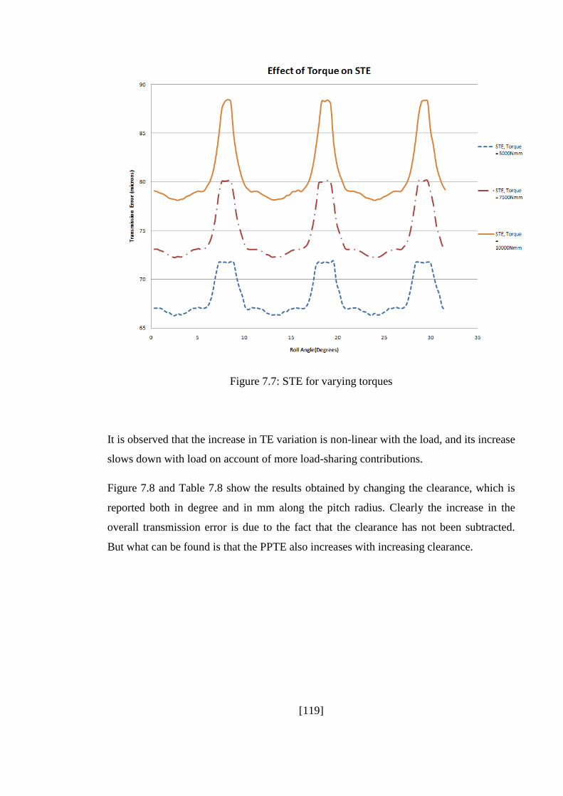
[119]
Figure 7.7: STE for varying torques
It is observed that the increase in TE variation is non-linear with the load, and its increase
slows down with load on account of more load-sharing contributions.
Figure 7.8 and Table 7.8 show the results obtained by changing the clearance, which is
reported both in degree and in mm along the pitch radius. Clearly the increase in the
overall transmission error is due to the fact that the clearance has not been subtracted.
But what can be found is that the PPTE also increases with increasing clearance.
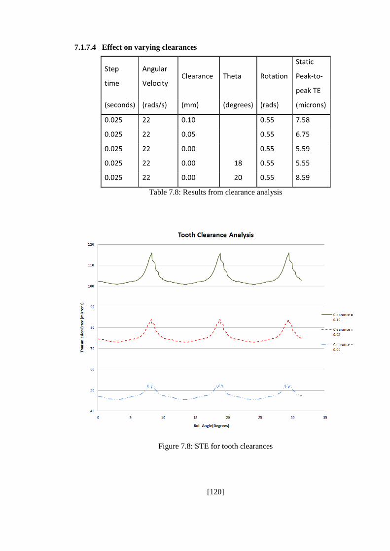
[120]
7.1.7.4 Effect on varying clearances
Step
time
Angular
Velocity Clearance Theta Rotation
Static
Peak-to-
peak TE
(seconds) (rads/s) (mm) (degrees) (rads) (microns)
0.025 22 0.10 0.55 7.58
0.025 22 0.05 0.55 6.75
0.025 22 0.00 0.55 5.59
0.025 22 0.00 18 0.55 5.55
0.025 22 0.00 20 0.55 8.59
Table 7.8: Results from clearance analysis
Figure 7.8: STE for tooth clearances

[121]
Figure 7.9 reports the variation of the TE as a result of the pressure angle used in the
design, and shows that the PPTE obtained for an angle of 18 deg is significantly lower
than that obtained for an angle of 22 deg.
Figure 7.9: STE for pressure angle
7.2 Hybrid numerical/analytical method
In this section, the hybrid numerical/analytical model described in Section 6 is used for
to analyse the same problem studied earlier in Section 7.1, with the specifications given
in Tables 7.1 and 7.2. Figure 7.10 reports a number of analyses conducted with the
hybrid numerical/analytical method and with two different values of damping, one
relatively low and one relatively high. In both cases the curves quickly converge within
about one tooth interaction to the curve obtained using a static analysis that is to the STE.
Therefore, the question which naturally arises is whether this result is due to the
approximation entailed by the numerical/analytical hybrid method or it is a correct result,
possibly general in the sense that is valid for many other designs of gears operating in
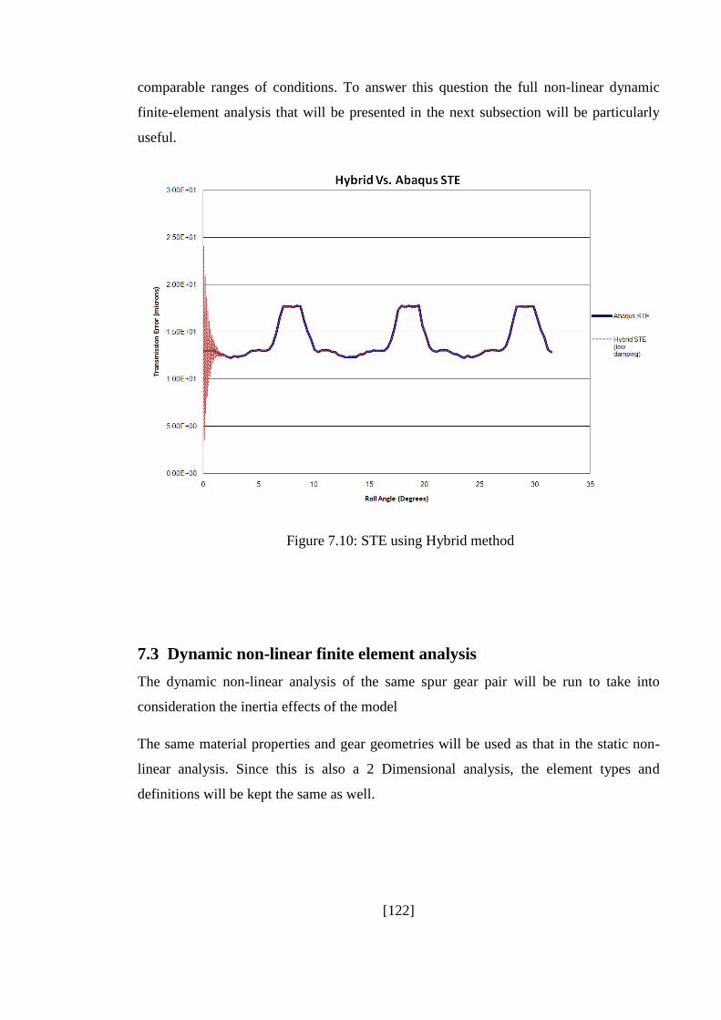
[122]
comparable ranges of conditions. To answer this question the full non-linear dynamic
finite-element analysis that will be presented in the next subsection will be particularly
useful.
Figure 7.10: STE using Hybrid method
7.3 Dynamic non-linear finite element analysis
The dynamic non-linear analysis of the same spur gear pair will be run to take into
consideration the inertia effects of the model
The same material properties and gear geometries will be used as that in the static non-
linear analysis. Since this is also a 2 Dimensional analysis, the element types and
definitions will be kept the same as well.
[123]
7.3.1 Analysis type
Abaqus offers us the choice of linear or nonlinear dynamic analysis, but in the case of
this work the dynamic analysis will be carried out on Abaqus including inertial effects
and the dynamic nonlinear system response to the input torque at the driving gear.
As described in Chapter 5, the steps for the implicit dynamic analysis were defined with
the gear system and operating conditions in mind. The implicit dynamic step named
rotation is defined and used to analyse the dynamic gear pair model, with a total time
period t, of 0.0025 seconds for the step and the whole analysis.
7.3.2 Interaction property
The interaction properties for the dynamic model were somewhat more complicated to
define. Initially the parameters used in the interaction property module were the same as
those used in the static analysis setup. The contact property for the surface to surface
contact between the mating faces of the respective gear teeth was set to normal
behaviour, with the pressure over-closure set to hard contact (Figure 7.11). Upon
running the dynamic implicit analysis, initially there were severe problems with
convergence of the two mating surfaces, resulting in the analysis aborting prematurely.
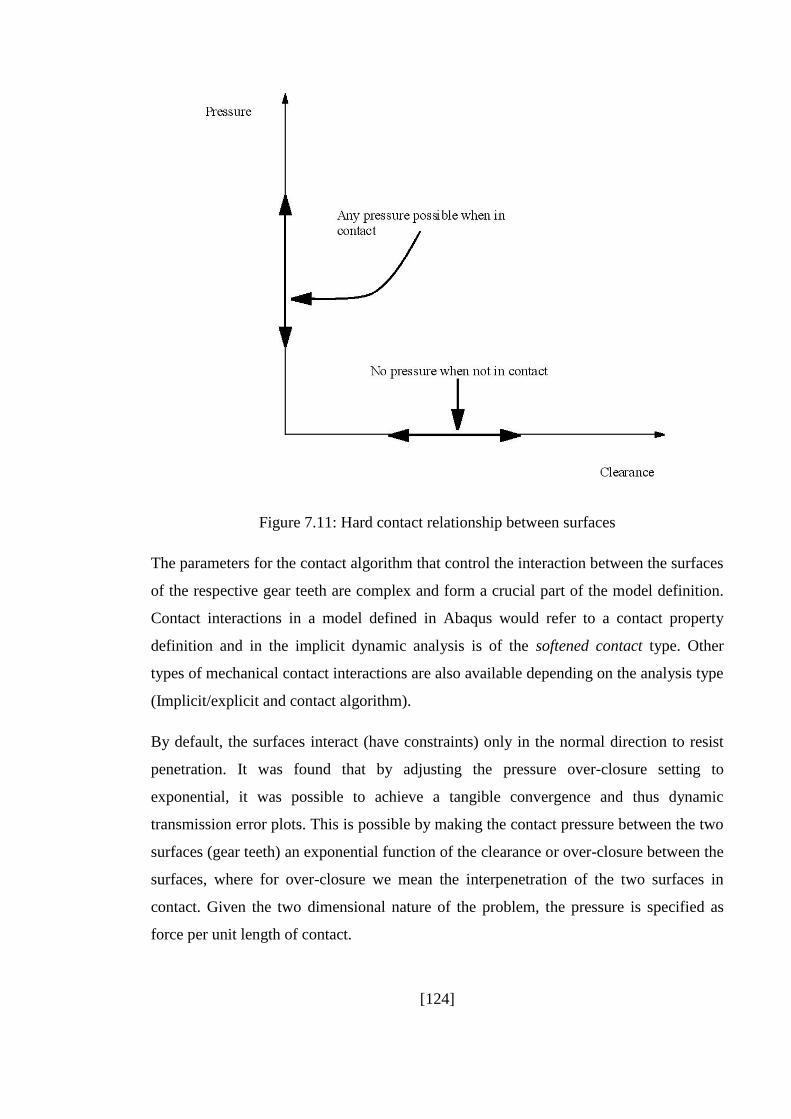
[124]
Figure 7.11: Hard contact relationship between surfaces
The parameters for the contact algorithm that control the interaction between the surfaces
of the respective gear teeth are complex and form a crucial part of the model definition.
Contact interactions in a model defined in Abaqus would refer to a contact property
definition and in the implicit dynamic analysis is of the softened contact type. Other
types of mechanical contact interactions are also available depending on the analysis type
(Implicit/explicit and contact algorithm).
By default, the surfaces interact (have constraints) only in the normal direction to resist
penetration. It was found that by adjusting the pressure over-closure setting to
exponential, it was possible to achieve a tangible convergence and thus dynamic
transmission error plots. This is possible by making the contact pressure between the two
surfaces (gear teeth) an exponential function of the clearance or over-closure between the
surfaces, where for over-closure we mean the interpenetration of the two surfaces in
contact. Given the two dimensional nature of the problem, the pressure is specified as
force per unit length of contact.
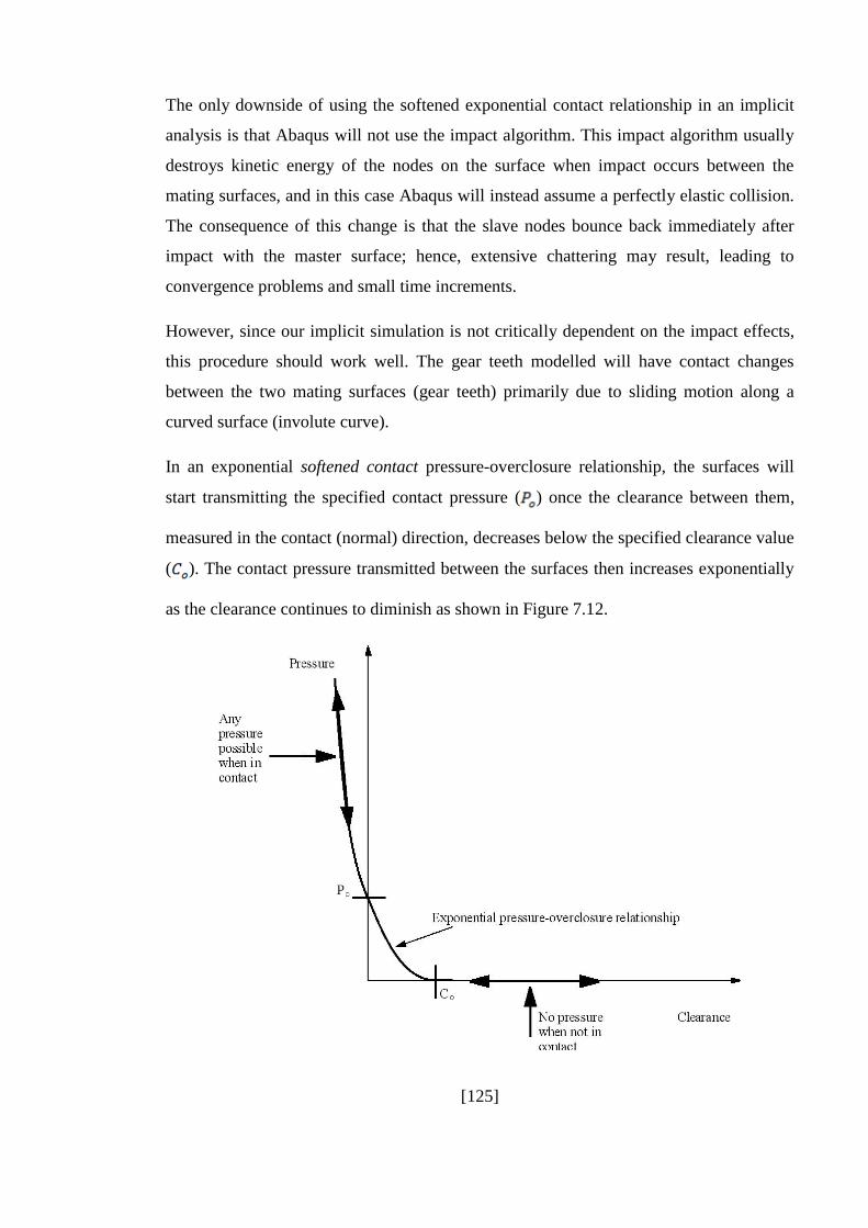
[125]
The only downside of using the softened exponential contact relationship in an implicit
analysis is that Abaqus will not use the impact algorithm. This impact algorithm usually
destroys kinetic energy of the nodes on the surface when impact occurs between the
mating surfaces, and in this case Abaqus will instead assume a perfectly elastic collision.
The consequence of this change is that the slave nodes bounce back immediately after
impact with the master surface; hence, extensive chattering may result, leading to
convergence problems and small time increments.
However, since our implicit simulation is not critically dependent on the impact effects,
this procedure should work well. The gear teeth modelled will have contact changes
between the two mating surfaces (gear teeth) primarily due to sliding motion along a
curved surface (involute curve).
In an exponential softened contact pressure-overclosure relationship, the surfaces will
start transmitting the specified contact pressure ( ) once the clearance between them,
measured in the contact (normal) direction, decreases below the specified clearance value
( ). The contact pressure transmitted between the surfaces then increases exponentially
as the clearance continues to diminish as shown in Figure 7.12.
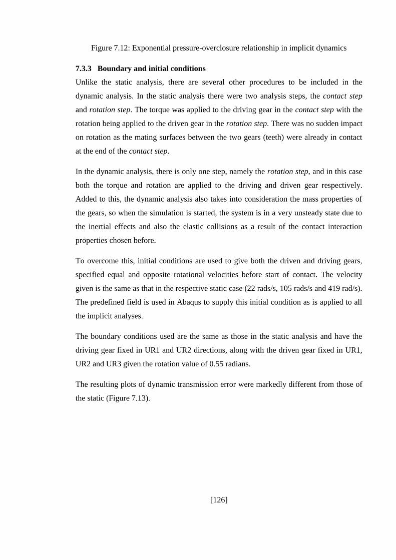
[126]
Figure 7.12: Exponential pressure-overclosure relationship in implicit dynamics
7.3.3 Boundary and initial conditions
Unlike the static analysis, there are several other procedures to be included in the
dynamic analysis. In the static analysis there were two analysis steps, the contact step
and rotation step. The torque was applied to the driving gear in the contact step with the
rotation being applied to the driven gear in the rotation step. There was no sudden impact
on rotation as the mating surfaces between the two gears (teeth) were already in contact
at the end of the contact step.
In the dynamic analysis, there is only one step, namely the rotation step, and in this case
both the torque and rotation are applied to the driving and driven gear respectively.
Added to this, the dynamic analysis also takes into consideration the mass properties of
the gears, so when the simulation is started, the system is in a very unsteady state due to
the inertial effects and also the elastic collisions as a result of the contact interaction
properties chosen before.
To overcome this, initial conditions are used to give both the driven and driving gears,
specified equal and opposite rotational velocities before start of contact. The velocity
given is the same as that in the respective static case (22 rads/s, 105 rads/s and 419 rad/s).
The predefined field is used in Abaqus to supply this initial condition as is applied to all
the implicit analyses.
The boundary conditions used are the same as those in the static analysis and have the
driving gear fixed in UR1 and UR2 directions, along with the driven gear fixed in UR1,
UR2 and UR3 given the rotation value of 0.55 radians.
The resulting plots of dynamic transmission error were markedly different from those of
the static (Figure 7.13).
[127]
Figure 7.13: Dynamic TE
The general shape of the static TE curve was close to the conventional plots by most
research publications, which indicate the rotation through the mesh of the pair of gear
teeth as the system is under operation.
The dynamic TE plot shown in figure 7.13 has two main differences, one being the
obvious oscillations between and , and the other being the higher amplitude of the
curve which is also smoother. The meshing frequency of the gear pair is the same as
would be expected, since none of the gear geometry was changed from the STE case.
It can also be observed that the handover of contact from one pair of meshed teeth to the
next begins earlier in the dynamic transmission error curve when compared to the static
case. This would suggest that there is a reduction of shared contact between the two gear
teeth and as a result an increase in vibration is likely.
At this time of the research work the hybrid numerical analytical method had not been
implemented yet and the initial thought was that for the chosen operating conditions the
DTE is indeed different from the STE. However, once the results were validated with the
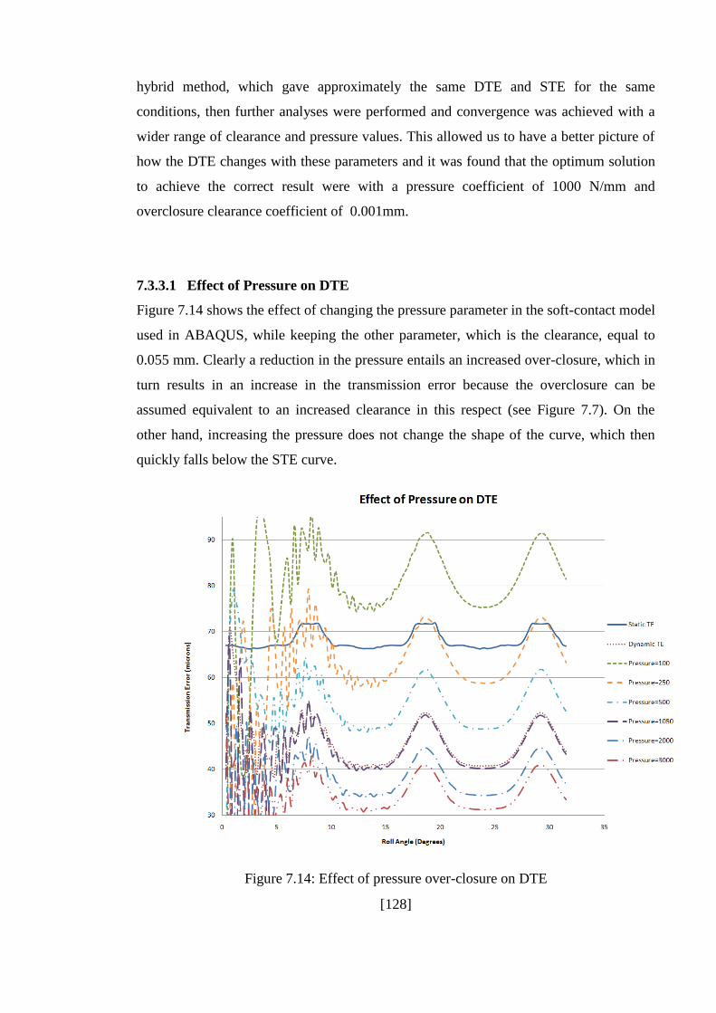
[128]
hybrid method, which gave approximately the same DTE and STE for the same
conditions, then further analyses were performed and convergence was achieved with a
wider range of clearance and pressure values. This allowed us to have a better picture of
how the DTE changes with these parameters and it was found that the optimum solution
to achieve the correct result were with a pressure coefficient of 1000 N/mm and
overclosure clearance coefficient of 0.001mm.
7.3.3.1 Effect of Pressure on DTE
Figure 7.14 shows the effect of changing the pressure parameter in the soft-contact model
used in ABAQUS, while keeping the other parameter, which is the clearance, equal to
0.055 mm. Clearly a reduction in the pressure entails an increased over-closure, which in
turn results in an increase in the transmission error because the overclosure can be
assumed equivalent to an increased clearance in this respect (see Figure 7.7). On the
other hand, increasing the pressure does not change the shape of the curve, which then
quickly falls below the STE curve.
Figure 7.14: Effect of pressure over-closure on DTE
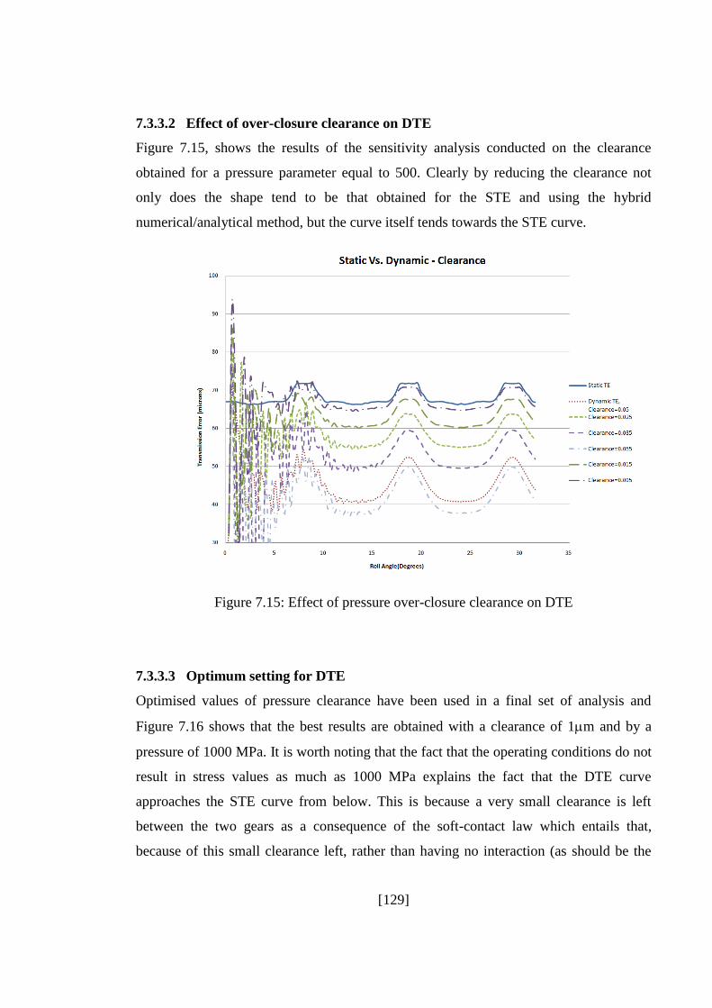
[129]
7.3.3.2 Effect of over-closure clearance on DTE
Figure 7.15, shows the results of the sensitivity analysis conducted on the clearance
obtained for a pressure parameter equal to 500. Clearly by reducing the clearance not
only does the shape tend to be that obtained for the STE and using the hybrid
numerical/analytical method, but the curve itself tends towards the STE curve.
Figure 7.15: Effect of pressure over-closure clearance on DTE
7.3.3.3 Optimum setting for DTE
Optimised values of pressure clearance have been used in a final set of analysis and
Figure 7.16 shows that the best results are obtained with a clearance of 1m and by a
pressure of 1000 MPa. It is worth noting that the fact that the operating conditions do not
result in stress values as much as 1000 MPa explains the fact that the DTE curve
approaches the STE curve from below. This is because a very small clearance is left
between the two gears as a consequence of the soft-contact law which entails that,
because of this small clearance left, rather than having no interaction (as should be the
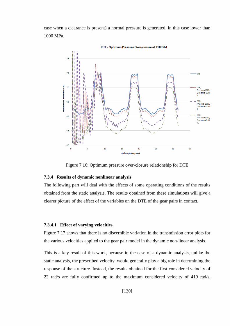
[130]
case when a clearance is present) a normal pressure is generated, in this case lower than
1000 MPa.
Figure 7.16: Optimum pressure over-closure relationship for DTE
7.3.4 Results of dynamic nonlinear analysis
The following part will deal with the effects of some operating conditions of the results
obtained from the static analysis. The results obtained from these simulations will give a
clearer picture of the effect of the variables on the DTE of the gear pairs in contact.
7.3.4.1 Effect of varying velocities.
Figure 7.17 shows that there is no discernible variation in the transmission error plots for
the various velocities applied to the gear pair model in the dynamic non-linear analysis.
This is a key result of this work, because in the case of a dynamic analysis, unlike the
static analysis, the prescribed velocity would generally play a big role in determining the
response of the structure. Instead, the results obtained for the first considered velocity of
22 rad/s are fully confirmed up to the maximum considered velocity of 419 rad/s,
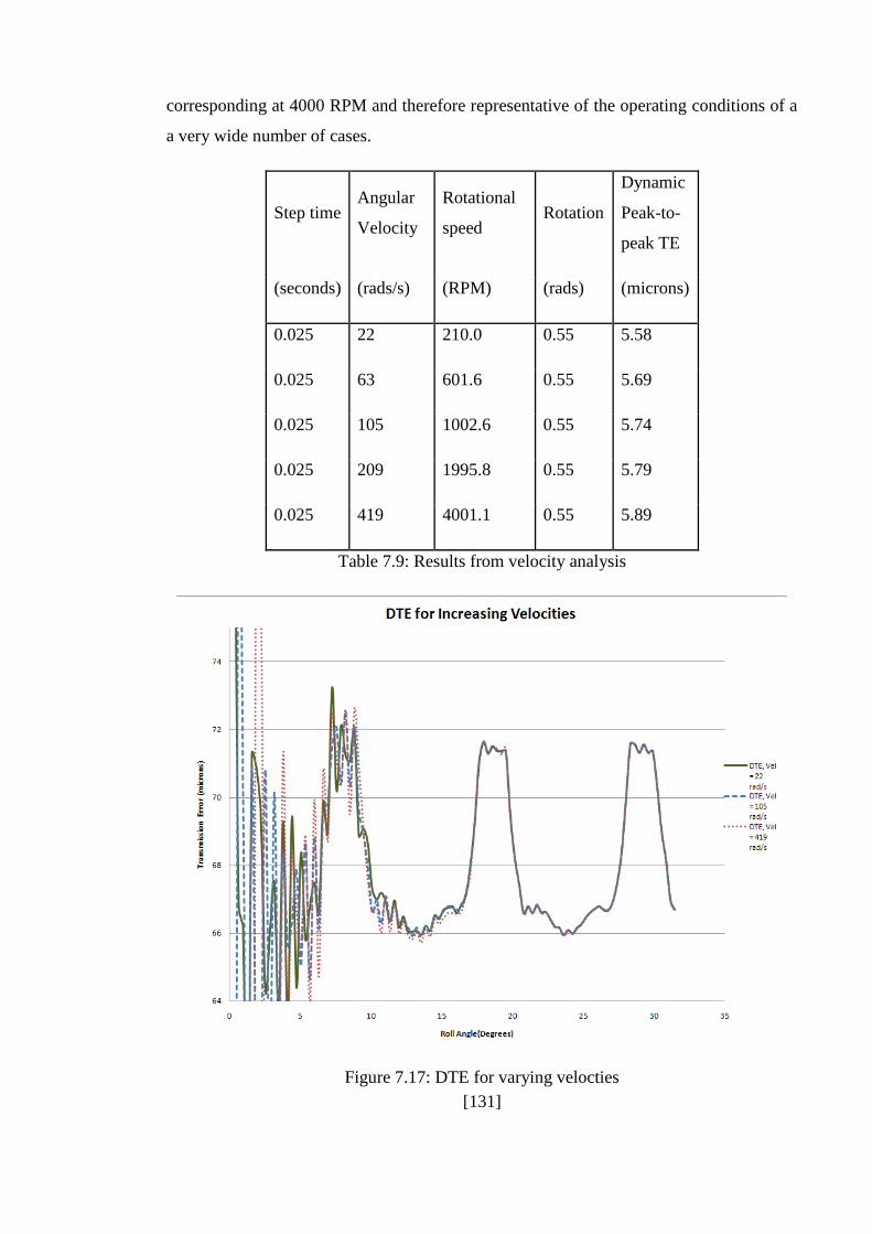
[131]
corresponding at 4000 RPM and therefore representative of the operating conditions of a
a very wide number of cases.
Step time Angular
Velocity
Rotational
speed Rotation
Dynamic
Peak-to-
peak TE
(seconds) (rads/s) (RPM) (rads) (microns)
0.025 22 210.0 0.55 5.58
0.025 63 601.6 0.55 5.69
0.025 105 1002.6 0.55 5.74
0.025 209 1995.8 0.55 5.79
0.025 419 4001.1 0.55 5.89
Table 7.9: Results from velocity analysis
Figure 7.17: DTE for varying velocties
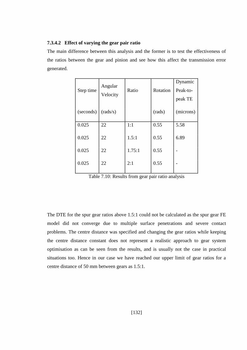
[132]
7.3.4.2 Effect of varying the gear pair ratio
The main difference between this analysis and the former is to test the effectiveness of
the ratios between the gear and pinion and see how this affect the transmission error
generated.
Step time Angular
Velocity Ratio Rotation
Dynamic
Peak-to-
peak TE
(seconds) (rads/s) (rads) (microns)
0.025 22 1:1 0.55 5.58
0.025 22 1.5:1 0.55 6.89
0.025 22 1.75:1 0.55 -
0.025 22 2:1 0.55 -
Table 7.10: Results from gear pair ratio analysis
The DTE for the spur gear ratios above 1.5:1 could not be calculated as the spur gear FE
model did not converge due to multiple surface penetrations and severe contact
problems. The centre distance was specified and changing the gear ratios while keeping
the centre distance constant does not represent a realistic approach to gear system
optimisation as can be seen from the results, and is usually not the case in practical
situations too. Hence in our case we have reached our upper limit of gear ratios for a
centre distance of 50 mm between gears as 1.5:1.
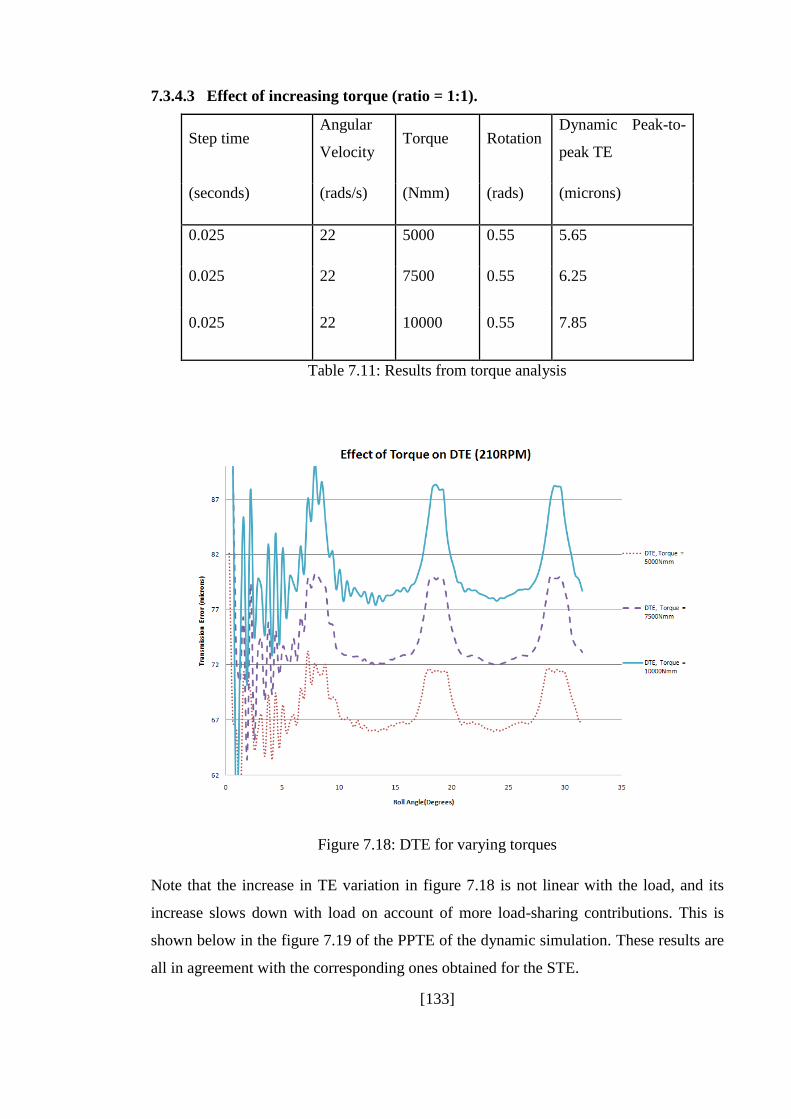
[133]
7.3.4.3 Effect of increasing torque (ratio = 1:1).
Step time Angular
Velocity Torque Rotation
Dynamic Peak-to-
peak TE
(seconds) (rads/s) (Nmm) (rads) (microns)
0.025 22 5000 0.55 5.65
0.025 22 7500 0.55 6.25
0.025 22 10000 0.55 7.85
Table 7.11: Results from torque analysis
Figure 7.18: DTE for varying torques
Note that the increase in TE variation in figure 7.18 is not linear with the load, and its
increase slows down with load on account of more load-sharing contributions. This is
shown below in the figure 7.19 of the PPTE of the dynamic simulation. These results are
all in agreement with the corresponding ones obtained for the STE.

[134]
Figure 7.19: Dynamic PPTE for varying torques
7.3.5 Effect of velocity input on DTE
The type of input given to the gear pair that is being simulating on Abaqus will
undoubtedly affect the outcome of the transmission error. In most applications of gear
pairs, such as those found in gear trains within transmission systems, the velocity is
always changing, and is never constant.
Even if it is to be assumed that the velocity input to the transmission system is constant,
the dynamical effects within the gear pair interacting with each other will combine to
bring about a change in this velocity. The TE caused by the contact between the teeth on
the first pair of gears (with constant velocity input) will cause accelerations and
decelerations of the driven gear, which is the driving gear for the second pair of gears,
and hence the resulting variation in the input to the next gear pair will cause the PPTE to
change in relation to the velocity.
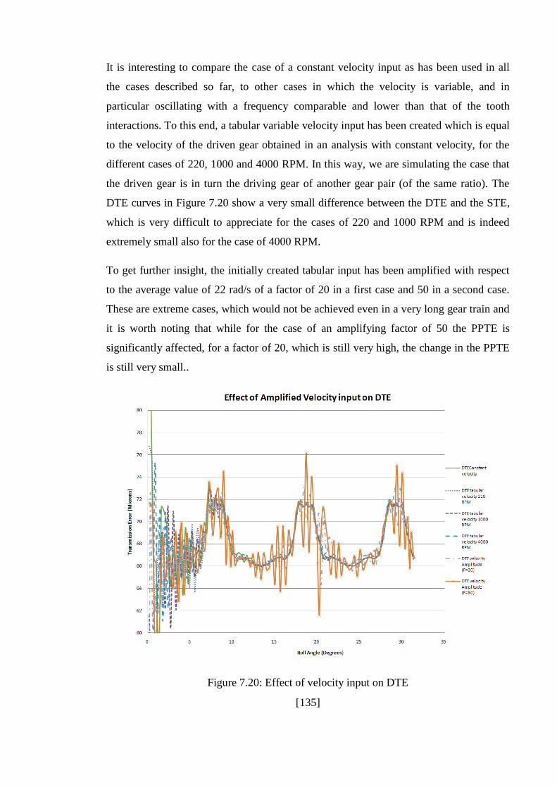
[135]
It is interesting to compare the case of a constant velocity input as has been used in all
the cases described so far, to other cases in which the velocity is variable, and in
particular oscillating with a frequency comparable and lower than that of the tooth
interactions. To this end, a tabular variable velocity input has been created which is equal
to the velocity of the driven gear obtained in an analysis with constant velocity, for the
different cases of 220, 1000 and 4000 RPM. In this way, we are simulating the case that
the driven gear is in turn the driving gear of another gear pair (of the same ratio). The
DTE curves in Figure 7.20 show a very small difference between the DTE and the STE,
which is very difficult to appreciate for the cases of 220 and 1000 RPM and is indeed
extremely small also for the case of 4000 RPM.
To get further insight, the initially created tabular input has been amplified with respect
to the average value of 22 rad/s of a factor of 20 in a first case and 50 in a second case.
These are extreme cases, which would not be achieved even in a very long gear train and
it is worth noting that while for the case of an amplifying factor of 50 the PPTE is
significantly affected, for a factor of 20, which is still very high, the change in the PPTE
is still very small..
Figure 7.20: Effect of velocity input on DTE
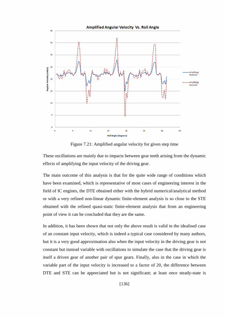
[136]
Figure 7.21: Amplified angular velocity for given step time
These oscillations are mainly due to impacts between gear teeth arising from the dynamic
effects of amplifying the input velocity of the driving gear.
The main outcome of this analysis is that for the quite wide range of conditions which
have been examined, which is representative of most cases of engineering interest in the
field of IC engines, the DTE obtained either with the hybrid numerical/analytical method
or with a very refined non-linear dynamic finite-element analysis is so close to the STE
obtained with the refined quasi-static finite-element analysis that from an engineering
point of view it can be concluded that they are the same.
In addition, it has been shown that not only the above result is valid in the idealised case
of an constant input velocity, which is indeed a typical case considered by many authors,
but it is a very good approximation also when the input velocity in the driving gear is not
constant but instead variable with oscillations to simulate the case that the driving gear is
itself a driven gear of another pair of spur gears. Finally, also in the case in which the
variable part of the input velocity is increased to a factor of 20, the difference between
DTE and STE can be appreciated but is not significant; at least once steady-state is

[137]
reached. The difference is instead significant when the amplifying factor for the variable
part of the velocity is 50. Even thought the simulation has been carried out at an
amplifying factor of 50, mainly to test the robustness of our process, in reality, this level
of amplification will not be seen by gear pairs in transmissions.
These results are extremely important and original because they have never been reported
in the wide literature of this field.
7.4 Explicit analysis
In concluding this chapter, it is worth noting that because of the extreme difficulty which
has been encountered in determining the parameters of the non-linear solution algorithm
in ABAQUS, significant time has been spent on exploring the possibility of conducting
explicit analysis, instead of implicit ones.
The use of explicit analysis could also be a way of performing speedy checks on the
effect of the tooth profile modifications on the TE of the spur gear pairs performed, as
the convergence problems faced when creating and running the implicit analysis would
not be faced. The same gear geometries were used and the following results were
obtained.
Figure 7.22: Spurious deflections in explicit models

[138]
The main problems encountered were the spurious deflections due to the large
displacements in the model in the radial direction which were not to be expected. The
rotational deflections caused the explicit model to crash and the tolerances need to
overcome this problem could not be met by the machines being used for the analysis. The
main reason for that is attributed to the inaccuracy in resolving the large strain
formulation in ABAQUS in a problem in which small errors accumulate instead of
cancelling out on average, because the rotational deformation and the overall symmetries
of this case.
[139]
8. GEAR PROFILE OPTIMISATION FOR STATIC
TRANSMISSION ERROR
In this chapter procedures for the optimization of profile modifications are developed to
reduce the rotational vibrations of a spur gear pair. Further research into the effect of
tooth profile modifications on the transmission error of gear pairs is carried out. The spur
gear pair was modelled using Abaqus under static conditions and the results obtained
were used to study the effect of intentional tooth profile modifications on the
transmission error of the gear pair. The use of a static analysis in this chapter is justified
by the results of Chapter 7, in which it was shown that for a significant range of
conditions of engineering interest the STE practically coincides with the DTE. A detailed
parametric study, involving development of an optimisation algorithm to design the tooth
modifications, is performed to quantify the changes in the transmission error as a
function of tooth profile modification parameters as compared to an unmodified gear pair
baseline. Plots of the STE are provided with respect to a couple of variables in order to
choose the set of them which yield to the minimum peak to peak STE and understand the
robustness of the system.
8.1 General approach to optimisation
The relationship between gears radiating noise and the transmission error has been
clarified and described in Chapter 3. For this reason, most approaches used by
researchers to create silent gears, are based on controlling and reducing the sources of
excitation such as STE and manufacturing errors.
The main concepts can be broadly divided into three categories:
8.1.1 Macro-geometry:
In this case the design process investigates the effect on radiated noise of macro-
geometrical parameters such as number of teeth, diameters, pressure angle, backlash, and
[140]
clearance. For example, many authors analyse the effects of involute contact ratio on both
spur and helical gears vibrations [56] suggesting values higher than two are preferable as
in the case of high contact ratio (HCR) gears. In a more detailed work, Kahraman [22-24]
quantified the influence of involute contact ratio on dynamic transmission error and
experimentally validate design guidelines to achieve quiet gears. Other related studies
give approximate equations for the relationship between pinion and gear addendum
modification factors to have a pre-established contact ratio considering also specific
sliding.
8.1.2 Surface refinement:
Since manufacturing profile errors are a possible source of dynamic excitation, the
quality of the teeth can affect gears vibrations. Important aspects such as surface
roughness, surfaces refinement and tolerance can play a significant role in reducing
radiated noise. The main problem related to increase the surface quality is due to higher
manufacturing cost.
8.1.3 Micro-geometry
In this case the main idea is to intentionally remove material from the gear tooth flanks
so that the resulting form is no longer a perfect involute. These modifications (tip and
root relief) compensate tooth deflections under load so that the resulting transmission
error is minimized for a particular range of operating conditions.
Since macro-geometry modifications can involve a drastic change of the gear pair, and it
is practicable only at the first steps of the design process, and surface refinements can
involve higher cost from a manufacturing point of view, the present work will focus its
attention only on micro geometrical optimization.
8.1.4 Harris Maps
The key point in designing the correct profile modifications is to reduce gears vibrations.
The literature offers many examples of guidelines to solve this problem but none of them
seems to be valid for all applications and load conditions.

[141]
In 1940 Walker was the first to consider the tooth deflection in calculation of tooth load.
He proposed a trapezoidal tooth cycle from which it was possible to calculate the amount
of tip relief and its extension along the tooth profile [4].
The major contributions in this field were given by the Harris [6] and Smith [40]. Harris
introduced the concept of static transmission error applied to profile modifications by
developing a unique diagram called “Harris map”.
Since a general profile modification can be represented as deviation from the theoretical
involute profile (see the example of Figure 11), the combined effect of one pair of teeth
meshing under no load would be to give a STE of the shape of Figure 8.1, with about a
third of total span following the involute for both profile and generating no error (in
Figure 8.1 the teeth has only tip relief).
Figure 8.1: Representation of STE for mating profiles with tip relief in case of no load.
If several pairs of teeth in mesh are putting in succession the obtained effect is the one of
Figure 8.2.
Figure 8.2: Effect of mating teeth pairs on STE in case tip relief and no-load.
The solid line of Figure 8.2 represents the STE under no-load conditions during gears
rotation. When load is applied there are two regimes (see Figure 8.3): one around the
pitch point where only one pair of teeth are in contact, one near the changeover points
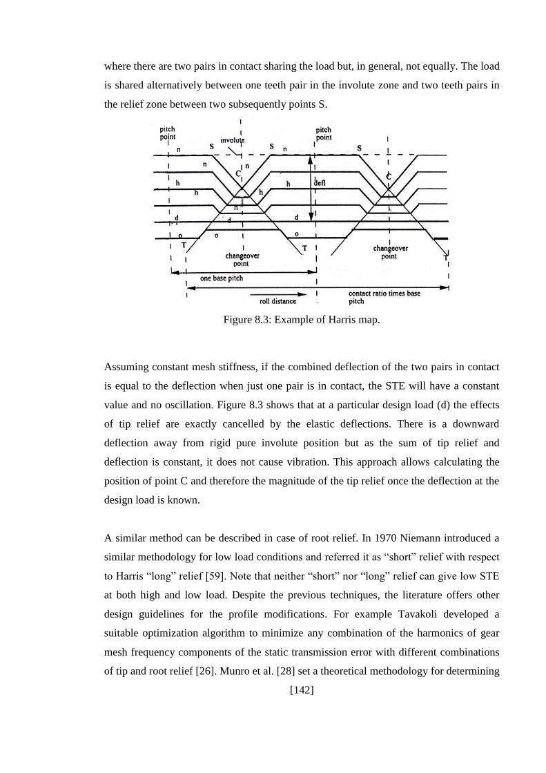
[142]
where there are two pairs in contact sharing the load but, in general, not equally. The load
is shared alternatively between one teeth pair in the involute zone and two teeth pairs in
the relief zone between two subsequently points S.
Figure 8.3: Example of Harris map.
Assuming constant mesh stiffness, if the combined deflection of the two pairs in contact
is equal to the deflection when just one pair is in contact, the STE will have a constant
value and no oscillation. Figure 8.3 shows that at a particular design load (d) the effects
of tip relief are exactly cancelled by the elastic deflections. There is a downward
deflection away from rigid pure involute position but as the sum of tip relief and
deflection is constant, it does not cause vibration. This approach allows calculating the
position of point C and therefore the magnitude of the tip relief once the deflection at the
design load is known.
A similar method can be described in case of root relief. In 1970 Niemann introduced a
similar methodology for low load conditions and referred it as “short” relief with respect
to Harris “long” relief [59]. Note that neither “short” nor “long” relief can give low STE
at both high and low load. Despite the previous techniques, the literature offers other
design guidelines for the profile modifications. For example Tavakoli developed a
suitable optimization algorithm to minimize any combination of the harmonics of gear
mesh frequency components of the static transmission error with different combinations
of tip and root relief [26]. Munro et al. [28] set a theoretical methodology for determining
[143]
the amount and extent of profile modifications to provide a smooth transmission error
curve when the module of the gear is higher than 5 mm. Cai and Hayashi [29] developed
an optimization technique by means of minimization of the equivalent exciting force.
Matsumura et al. [60] and Rouverol [61] defined new methodologies to eradicate gears
noise through profile deviations, respectively for light and high load conditions.
Experimental works were made by Kahraman and Blankenship [23] who analyzed the
influence of gears linear flank modifications on the rotational vibrations of a spur gears
system by means of measured DTE.
8.1.5 Profile modification
The two main methods currently being implemented, in order to reduce the gear noise
and vibration response of the system are by means of macro-geometry and micro-
geometry modifications.
Macro-geometry is defined by gear parameters such as: number of teeth, diameters,
pressure angle, backlash and clearance. Many authors studied the effect of the involute
contact ratio on both spur and helical gear vibrations [17-18]. Macro-geometric
modifications involve an important and expensive change of the gear pair as well as the
other members of the gear train; they are feasible only at the first steps of the design
process. High quality surface finishing and strict tolerances can lead to excessive
manufacturing costs; moreover, their effect on vibrations can be disappointingly small.
Micro-geometric modifications consist in an intentional removal of material from the
gear teeth flanks, so that the resulting shape is no longer a perfect involute; such
modifications compensate teeth deflections under load, so that the resulting transmission
error is minimized for a specific torque [2]. Therefore in this study, the micro-geometry
modifications will be the focus of the analysis.

[144]
8.1.6 Finite element model
The optimization design in this chapter starts from the results obtained in Chapter 7 by
exploring the possibility of adding an addendum or a dedendum modification. The quasi-
static analysis has been done for each the proposed design. The results in terms of
contour plot of the von Mises stress are showed in Figure 7.4.
Details of the implementation are given in the Python routines which are reported in the
Appendix.
Figure 8.4: FE gear pair mesh
This analysis is run once for a given macro-geometry which requires essential input
details such as number of teeth, module, tooth depth, addendum and dedendum radii,
modifications and pitch circle diameter etc. The preprocessor in the FEA software
automatically generates the FE model of the two gears, and an internal FE solver
generates the compliance and stress coefficients.
The second part of the procedure involves a tooth contact analysis (TCA), which is run
repeatedly to optimize the micro-geometry modification in order to achieve minimum TE

[145]
and gear stress. This requires input details relevant to the modification being made, such
as root relief, profile crowning, lead correction, end relief, face crowning, or any defined
surface topography, in the case of this study it is tip relief. As this part of the method
requires very little computational time, the calculations can be repeated with varying
geometry to achieve minimum TE and stress. The output from the calculation procedure
yields the STE, tooth load, and contact and bending stress as a distribution across the
face width at a particular phase mesh between the gears.
8.1.7 Profile modification algorithm
For a first study, the gear micro-geometry modification for the tooth profile is the tip
relief (Figure 8.5). This modification is very important for proper gear mesh and
engagement process, especially when assembly deflection is significant. For the mating
pair of teeth under load, it is not possible to have the next tip enter contact in the pure
involute position because there would be sudden interference corresponding to the elastic
deflection and the corner of the tooth tip would gouge into the mating surface [2].
Manufacturing errors can add to this effect, which is the main reason to relieve the tooth
tip and ensure that the corner does not dig in.
Figure 8.5: Spur gear tooth profile modification

[146]
Since this first part deals with the optimization of one variable, i.e. tip relief, which is
called “addmod”, it is quite straightforward to choose an algorithm to determine the
minimum value for the parameter. The primary differences between algorithms (steep
descent, Newton’s method, Fibonacci, etc.) lies with the rule by which successive
directions of movements are chosen. Once this direction is selected, all algorithms call
for movement to the minimum point on the corresponding line. This process of
determining the minimum point on a given line (one variable) is called line search. The
kind of algorithm selected for this study is called the Fibonacci method and is a very
popular method for resolving the line search problem. The only property that is to be
assumed of this f (variable/parameter), “addmod” in this case, is that it must be unimodal,
i.e. it must have a single relative minimum [30].
8.2 Optimisation algorithms
As seen from the results in Chapter 7, the effect of velocities on the STE and DTE is
negligible and hence can be ignored with respect to the optimisation procedure. Chapter
7 also provides results that summarise that the STE and DTE are identical if modelled
appropriately on the FE model with respect to the interaction properties. The TE curves
for the static and dynamic curves also exhibit an identical linear relationship due the
effect of increasing torque on the gear pair.
Therefore it is the object of this section of work to optimise the profile of the respective
spur gear pair for the operating torque of and will not be repeated for further
torque values as the linear trend will most likely carry over into the optimisation
procedure.
The process of obtaining the optimum gear tooth profile for the required spur gear pair is
two folded. The first part of this work focuses on the one parameter optimisation of the
spur gear tooth profile, where the tip of the involute curve is modified with a linear relief.
The second part of the work will develop the two parameter optimisation procedure for
the same spur gear pair, with respect to the tip and root portions of the involute curve.
The tip and root modification to the involute profile will once again be linear.

[147]
The choice of linear or parabolic relief to the profile was one that had to be taken early
on in the work. It is well known from literature [11] that the short stubby gear teeth of
spur gears display elastic behaviour and produce significant deflections under loading.
This is mainly due to the non-linear Hertzian contact deflections coupled with the general
tooth movement, which makes the spur gear tooth act as a short cantilever beam. Gregory
et al. [11] used a figure of for the approximate mesh stiffness of a typical
spur gear tooth, which has stood the test of time since the late 1950s.
As the gears rotate through their mesh, the stiffness of each tooth varies greatly from the
tip to the root and for a pair of interacting teeth with shared geometries, this effect is
cancelled. In practice, for a pair of running spur gears, it is highly unlikely for the applied
load to be even across the face width of the gear tooth. As a result, the ends of the gear
tooth must be designed to allow for overloading and deflection.
8.3 One parameter optimisation
Due to the need to optimise the tooth fillet of only a single gear at a time to evaluate the
effect on the overall transmission error of the gear system, a one parameter optimisation
procedure was developed on Matlab. It uses the basic principle of the Newton’s steepest
descent algorithm, where by the equations to be solved are done so in a solutions space
with the objective function already defined. As the solution of the equations get closer to
the objective function, the solution space is redefined making it more accurate than the
previous iterations of calculations. This process is repeated until the solution to the
equations is within a specified tolerance (as in our case) or a unique solution is reached.
8.4 Main reasons for tip relief
As it has been established in the previous section that the mating teeth of a gear undergo
deflection under load, it is not advisable to have the next mating teeth enter contact in a
pure involute position. If this were to occur, the tips of the next mating pair of teeth
would cause interference with respect to the overall deflection and the corner of the tooth
tip would gouge into the mating surface. If this were to happen over a period of the
operating cycle, the resulting loss of material will cause fatigue and ultimately failure of
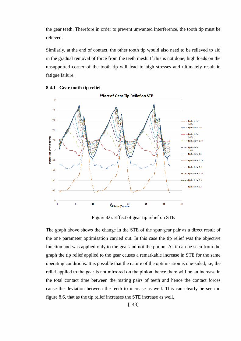
[148]
the gear teeth. Therefore in order to prevent unwanted interference, the tooth tip must be
relieved.
Similarly, at the end of contact, the other tooth tip would also need to be relieved to aid
in the gradual removal of force from the teeth mesh. If this is not done, high loads on the
unsupported corner of the tooth tip will lead to high stresses and ultimately result in
fatigue failure.
8.4.1 Gear tooth tip relief
Figure 8.6: Effect of gear tip relief on STE
The graph above shows the change in the STE of the spur gear pair as a direct result of
the one parameter optimisation carried out. In this case the tip relief was the objective
function and was applied only to the gear and not the pinion. As it can be seen from the
graph the tip relief applied to the gear causes a remarkable increase in STE for the same
operating conditions. It is possible that the nature of the optimisation is one-sided, i.e, the
relief applied to the gear is not mirrored on the pinion, hence there will be an increase in
the total contact time between the mating pairs of teeth and hence the contact forces
cause the deviation between the teeth to increase as well. This can clearly be seen in
figure 8.6, that as the tip relief increases the STE increase as well.
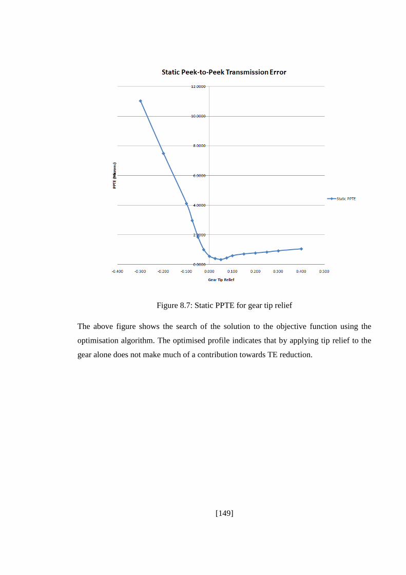
[149]
Figure 8.7: Static PPTE for gear tip relief
The above figure shows the search of the solution to the objective function using the
optimisation algorithm. The optimised profile indicates that by applying tip relief to the
gear alone does not make much of a contribution towards TE reduction.
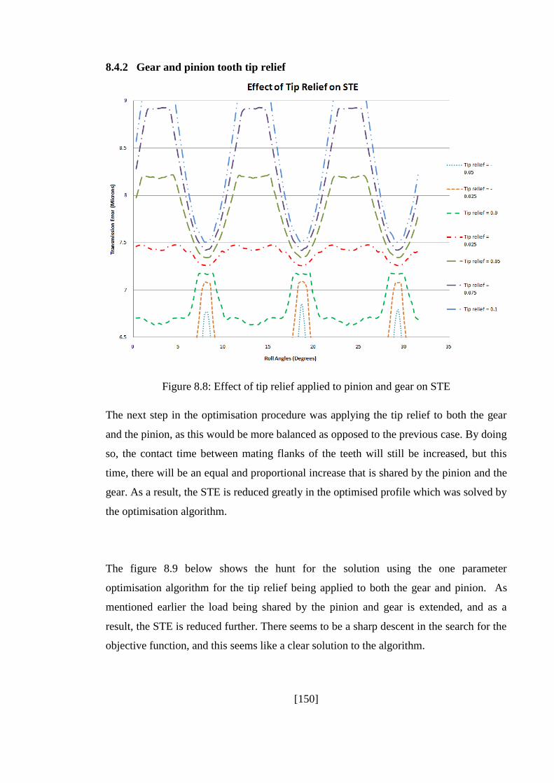
[150]
8.4.2 Gear and pinion tooth tip relief
Figure 8.8: Effect of tip relief applied to pinion and gear on STE
The next step in the optimisation procedure was applying the tip relief to both the gear
and the pinion, as this would be more balanced as opposed to the previous case. By doing
so, the contact time between mating flanks of the teeth will still be increased, but this
time, there will be an equal and proportional increase that is shared by the pinion and the
gear. As a result, the STE is reduced greatly in the optimised profile which was solved by
the optimisation algorithm.
The figure 8.9 below shows the hunt for the solution using the one parameter
optimisation algorithm for the tip relief being applied to both the gear and pinion. As
mentioned earlier the load being shared by the pinion and gear is extended, and as a
result, the STE is reduced further. There seems to be a sharp descent in the search for the
objective function, and this seems like a clear solution to the algorithm.
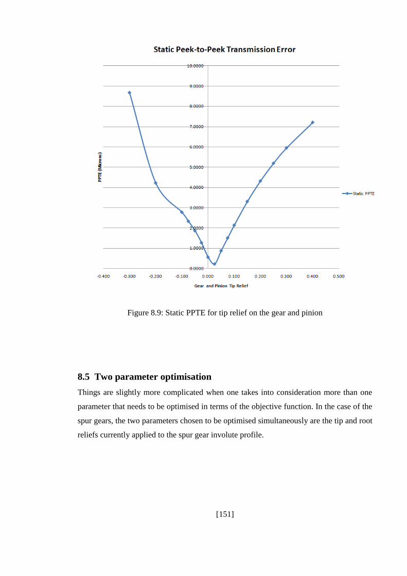
[151]
Figure 8.9: Static PPTE for tip relief on the gear and pinion
8.5 Two parameter optimisation
Things are slightly more complicated when one takes into consideration more than one
parameter that needs to be optimised in terms of the objective function. In the case of the
spur gears, the two parameters chosen to be optimised simultaneously are the tip and root
reliefs currently applied to the spur gear involute profile.
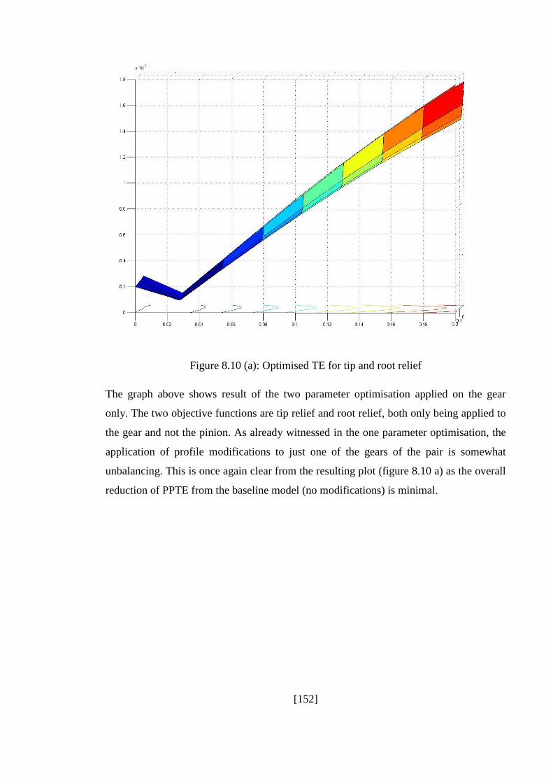
[152]
Figure 8.10 (a): Optimised TE for tip and root relief
The graph above shows result of the two parameter optimisation applied on the gear
only. The two objective functions are tip relief and root relief, both only being applied to
the gear and not the pinion. As already witnessed in the one parameter optimisation, the
application of profile modifications to just one of the gears of the pair is somewhat
unbalancing. This is once again clear from the resulting plot (figure 8.10 a) as the overall
reduction of PPTE from the baseline model (no modifications) is minimal.
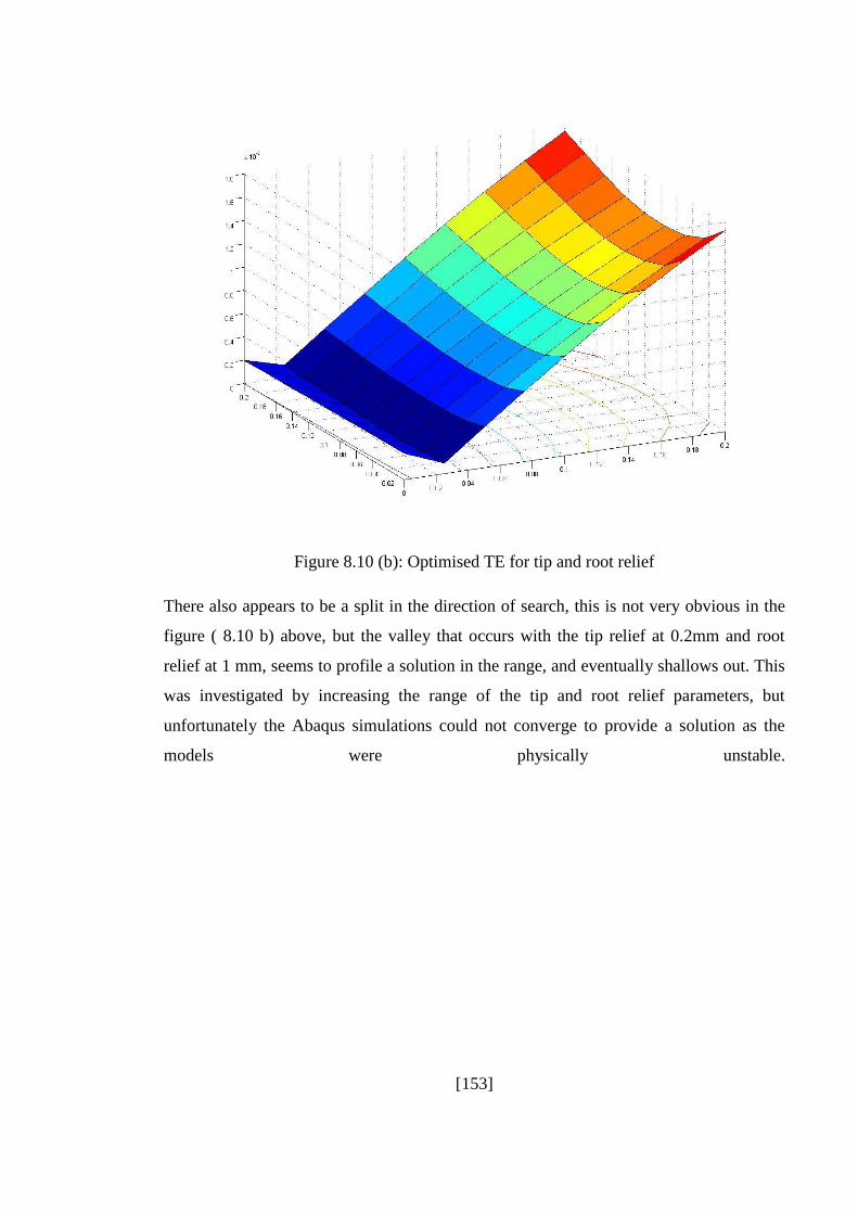
[153]
Figure 8.10 (b): Optimised TE for tip and root relief
There also appears to be a split in the direction of search, this is not very obvious in the
figure ( 8.10 b) above, but the valley that occurs with the tip relief at 0.2mm and root
relief at 1 mm, seems to profile a solution in the range, and eventually shallows out. This
was investigated by increasing the range of the tip and root relief parameters, but
unfortunately the Abaqus simulations could not converge to provide a solution as the
models were physically unstable.
[154]
9. CONCLUSIONS AND RECOMMENDATIONS
9.1 Conclusions
The work carried out in the field of gear research has been continuously evolving since
its conception over 3000 years ago. In this research, the work mainly revolved around the
concept of transmission error and its effect on the perceived noise radiation from the gear
interactions. Transmission error has been synonymous with gear design since it was
introduced by Harris [6] in 1958 and hence forth developed by numerous researchers in
the last few decades. By using the established definition of TE as the focal point of the
research, it was possible to isolate one of the main causes of gear noise and in turn
identify it as one of the main objective function of our optimisation procedure.
A spur gear pair modelled using finite elements was simulated and analysed under static
conditions. The results obtained were used to study the effect of intentional tooth profile
modifications on the transmission error of the gear pair, leading to a detailed parametric
study, involving development of an optimisation algorithm to design the tooth
modifications. The parameterised changes were quantified in terms of transmission error
as a function of tooth profile modification parameters and compared to an unmodified
gear pair baseline. The work also investigated the main differences between the static and
dynamic transmission error generated during the meshing of a spur gear pair model while
using FE software (Abaqus) and also verified this with the use of a hybrid
numerical/analytical model. This combination of Finite-Element Analysis, hybrid
numerical/analytical methodology and optimisation algorithms were used to scrutinise
the dynamic behaviour of the gear pairs under various operating conditions and loading.
The work carried out within this thesis shows that the hybrid results are identical to the
FE results obtained using Abaqus, both for the static and dynamic cases. This has been
shown to be due to the method used in defining the hybrid approach, by using the static
TE data gathered after analysis on Abaqus. The static and dynamic analysis carried out
[155]
reveals the differences between the static and dynamic TE is minimal, and mainly due to
the damping conditions that are prevalent in the dynamic analysis. As opposed to what
would be intuitively suggested when modelling a dynamic problem, the results obtained
seem somewhat to defy this logic. The main outcomes from the FE model suggest that
the contact properties within the dynamic model of the spur gear pair are to play a major
factor in determining the outcome of the transmission error. The single parameter
optimisation used to accurately identify the optimum tip relief coefficient for the spur
gear profile has been developed by using Matlab code and implemented in conjunction
with Abaqus within the iteration loop of the algorithm. The results show that the tip relief
does make a significant impact on the PPTE generated of a spur gear pair. The two
parameter optimisation algorithm which is also developed in Matlab uses the tip relief
and root relief of the spur gear profile to find the optimal profile for minimum PPTE for
the given gear pair. The results indicate that the root relief does not have as much of an
influence on the PPTE of the spur gear pair as the tip relief does.
The section below shows the main contributions to the field of research and summarises
the pertinent achievements as related to the objectives set out at the start of the research.
9.1.1 Comparison between STE and DTE
One of the main contributions of this work to the field of research is the comparison
between STE and DTE in identical gear pairs. This research for the first time brings
together a direct comparison between the effect of profile modifications on the STE and
DTE of spur gear pairs. The major finding is slightly surprising and unexpected as there
seems to be no major difference between the peak-to-peak TE of the static and dynamic
cases. This goes again the intuition that as a dynamic case is considered, the inertial
properties along with the higher loads would impose a higher TE. This is definitely not
the case, and has been demonstrated in Chapter 7 where the major conditions affecting
the DTE results were interrogated.
9.1.2 Full non-linear dynamic finite-element analyses of gear pair interaction
The non-linear simulation of a fully defined spur gear has been successfully carried out
and results analysed to obtain meaningful correlation between STE and DTE. The non-

[156]
linear simulation posed a slight problem in terms of achieving accuracy in the face of
convergence problems whilst using the FE software. The reasoning to attempt both
implicit and explicit analyses proved insightful, as the more accurate implicit simulations
was coxed to convergence by fine-tuning the operational parameters, whilst the explicit
simulations were far from converging to give a meaningful result. The spurious
deformations affecting both spur gears in the explicit simulations proved a hurdle too far
to overcome in this research.
9.1.3 Validation of our FE model using the Hybrid numerical model
The hybrid numerical/analytical model of the spur gear pair model system was developed
using equations of motion and the formulation for the transmission error derived. The
gear model developed in chapter 6 is an established two-degree-of-freedom (dof) gear
model modified to suit the methodology of this research as explained in chapter 6. The
results from the numerical simulation of the gear model, validate the finding of the FE
software. The STE from the Abaqus simulation was used to define several important
properties of the numerical model and run to calculate the generated DTE of the gear
model. The findings from this approach show that there is a strong correlation between
the STE results from the FE software and the DTE results from the hybrid approach.
9.1.4 Application of the automated profile modification tool to reduce TE
The use of an automated profile generation tool along with the automated profile
modification tool greatly helped in the increased efficiency of this research. The novel
idea to use python scripts to make all necessary macro and micro geometry changes to
the spur gear pair was profoundly successful. The main micro geometrical changes made
to the spur gears were the intentional teeth modifications in terms of tip and root relief.
The respective parameter modification plots shown in Chapter 7 shown the effects of
these on the STE and DTE of the spur gear pair.
The automated profile modification tool was used complimentarily with a MATLAB
routine which made use of the one and two parameter optimisation codes. The one
parameter optimisation made use of the tip or root relief to find the optimised spur gear
[157]
tooth profile that provided the lowest TE for gear and pinion respectively. The two
parameter optimisation tool was used to change both the tip and root relief of the spur
gear tooth in order to find the optimised shape that gave the lowest STE and DTE for the
gear and pinion respectively.
9.2 Recommendations for future work
The major recommendations that can be made for future work in this field of gear
research are mainly based on the continuation of the current approach. The current hybrid
numerical/analytical gear model can be further developed to allow for more degrees of
freedom, in order to achieve a more realistic representation of the spur gear system.
Finite element simulations carried out in this thesis were solely based on the 2D model of
spur gear pair generated using the automated profile generation tool. In future this could
be further expanded to include a 3D model of the spur gear pair to start with, followed by
a more complete 3D model including shafts and bearings. Another major addition could
be the use of a frictional coefficient and analyse the effects of this variable in terms of
variations in results in 2D and 3D TE.
Finally, the optimisation procedures used for the one and two parameter modification of
the spur gear teeth were quite crude as they used very simple algorithms as they were
based on a simple linear search. As this is a major factor in the search the optimised
objective function, use of more advanced algorithms based on reduction and
deterministic techniques will be researched.
The use of high-level programming languages to automate the once tedious tasks of
repetitive geometrical modelling and analysis has been a success. In particular, the
modelling tool developed in this project allows us to assimilate very refined FE
simulations with well established design optimisation algorithms in a much more
effective method with respect to what has already been presented in the research field.
[158]
REFERENCES
[1] B. Challen and R. Baranescu, Diesel Engine Reference Book. 2nd
Edition, The Bath
Press, Bath, 1999.
[2] J. C. Huang and K. R. Abram, Cummins 4B Noise Reduction Anti-Backlash
Camshaft Gear. Proceedings of the 1999 Noise and Vibration Conference, SAE
paper 1999-01-1761.
[3] H. Zhao and T. E. Reinhart, The Influence of Diesel Engine Architecture on Noise
Levels. Proceedings of the 1999 Noise and Vibration Conference, SAE paper 1999-
01-1747.
[4] H. Walker, Gear tooth deflections and profile modifications, Engineer, 170 (1940),
pp. 102–104.
[5] R.W. Gregory, S.L. Harris, R.G. Munro, Torsional motion of a pair of spur gears.
Proceedings of the Institution of Mechanical Engineers, 1963.
[6] S.L. Harris, Dynamic loads on the teeth of spur gears, Proceedings of the Institution
of Mechanical Engineers, 172 (2) (1958), pp. 87–100.
[7] H. Özgüvent, and D. Houser, Mathematical models used in gear dynamics – a
review. Journal of Sound and Vibration, 1988, 121(3), 384–411.
[8] J.D. Smith, Gears and theirs vibration, A Basic Approach to Understanding Gear
Noise. The Macmillan Press LTD., 1983.
[9] D. B. Welbourn, Fundamental knowledge of gear noise – A survey. In IMechE
Conference on Noise and Vibrations of Engines and Transmissions 1979, Cranfield,
10–12 July 1979, Conference Publications 1979-10, paper C117/79, pp. 9–14
[10] H. K. Kohler, A. Pratt, and A. M. Thompson, Dynamics and noise of parallel axis
gearing. IMechE Gearing Conference, Cambridge, 1970, pp. 111–121.
[159]
[11] R.W. Gregory, S.L. Harris, R.G. Munro, Dynamic behaviour of spur gears.
Proceedings of the Institution of Mechanical Engineers, 1963.
[12] M. MackAldener, Tooth Interior Fatigue Fracture & Robustness of Gears, Royal
Institute of Technology, Stockholm, Doctoral thesis, 2001, ISSN 1400-1179.
[13] R. Maliha, U.C. Dogruer and H.N. Ozguven, Nonlinear dynamic modeling of gear-
shaft-disk-bearing systems using finite elements and describing functions, Journal of
Mechanical Design 126, 2004, pp. 534–541
[14] P. Velex, and M. Ajmi, On the modelling of excitations in geared systems by
transmission errors. Journal of Sound and Vibration, 290, 2006, 882-909
[15] R. G. Munro, A review of the theory and measurement of gear transmission error.
Proceedings of the First IMechE Conference on Gearbox Noise and Vibration,
paper C404/032, 1990, pp. 3–10
[16] R. G. Munro, Optimum profile relief and transmission error in spur gears.
Proceedings of the First Institution of Mechanical Engineers International
Conference on Gearbox Noise and Vibration, Cambridge, 1990
[17] D. R. Houser, F. B. Oswald, M. J. Valco, R. J. Drago, and J. W. Lenski, Comparison
of transmission error predictions with noise measurements for several spur and
helical gears. In Proceedings of 30th AIAA, SAE, and ASEE Propulsion Conference,
Indianapolis, June 1994, AIAA-94-3366, pp. 1–16.
[18] F. Kayama, The Dynamics of Parallel Axis Gears in an Automotive Transmission.
PhD Thesis, University of Leeds, 2005.
[19] M. Beghini, F. Presicce, C. Santus, A method to define profile modification of spur
gear and minimize the transmission error, AGMA Technical Paper, 04FTM3, 2004.
[20] D. Houser, Gear noise state of the art. CETIM Internoise 88, Avignon, 1988, vol. 2,
pp. 601–606
[21] R. G. Parker, Progress and problems in gear vibration and noise. Second
International Conference on Damping technologies, Army Research Lab Workshop
9302-AN-03, Stellenbosch, South Africa, April 2003, p. 13.
[160]
[22] G. W. Blankenship, and A. Kahraman, Gear dynamics experiments; part I –
characterization of forced response. ASME Power Transmission & Gearing
Conference, San Diego, 1996, pp. 373–380.
[23] A. Kahraman, and G. W. Blankenship, Effect of involute tip relief on dynamic
response of spur gears. ASME Journal of Mechanical Design., 1999, 121, pp. 313–
315
[24] A. Kahraman, and G. W. Blankenship, Effect of involute contact ratio on spur gear
dynamics. ASME Journal of Mechanical Design., 1999, 121, pp. 112–118
[25] T. Sato, K. Umezawa, and J. Ishikawa, 1983. Effects of contact ratio and profile
correction on gear rotational vibration. Bullettin of the JSME, 26, pp. 2010–2016.
[26] M. Tavakoli, and D.Houser, 1986. Optimum profile modifications for the
minimization of static transmission errors of spur gears. Journal of Mechanism,
Transmissions and Automation in Design, 108, pp. 86–95
[27] V. Simon, Optimal tooth modifications for spur and helical gears. Journal of
Mechanism, Transmissions, and Automation in Design, 1989. 111, pp. 611–615
[28] R. Munro, N. Yildirim, and D. Hall, Optimal profile relief and transmission error in
spur gears. In ASME International Power Transmission and Gearing Conference,
1990. Vol. 111, pp. 611–615
[29] Y. Cai, and T Hayashi, The optimum modification of tooth profile for a pair of spur
gears to make its rotational vibration equal zero. In ASME International Power
Transmission and Gearing Conference, 1992. Vol. 43, pp. 453–460
[30] D. J. Fonseca, S. Shishoo, T. Lim, and D. Chen, A genetic algorithm approach to
minimize transmission error of automotive spur gear sets. Applied Artificial
Intelligence 19, 2005. pp. 153–179
[31] A. Toda and M. Botman, Planet Indexing in Planetary Gears for Minimum
Vibration, ASME paper, 79-DET-73
[32] W. Li, F. Gu, A. Ball, A. Leung and C. Phipps, A Study of the Noise from Diesel
Engines Using the Independent Component Analysis, Mechanical Systems and
Signal Processing, 2001, 15(6), 1165-1184.
[161]
[33] Y. Maetani, T. Niikura, S. Suzuki, S. Arai and H. Okamura, Analysis and Reduction
of Engine Front Noise Induced by the Vibration of the Crankshaft System,
Proceedings of the 1993 Noise and Vibration Conference, SAE Technical Paper
931336.
[34] S. Shih, J. Yruma and P. Kittredge, Drivetrain Noise and Vibration Troubleshooting,
International Truck and Bus Meeting and Exhibition, November 12-14, 2001, SAE
Technical Paper 2001-01-2809
[35] D. Houser, J. Harianto, J. Sorenson, T. Lim, C. Myers, B. Gordon and S. Berry,
Case History: Engine Timing Gear Noise Reduction, Proceedings of the 1999 Noise
and Vibration Conference, SAE Technical Paper 1999-01-1716.
[36] Y. Miura and S. Nakamura, Gear rattling noise analysis for a diesel engine.
European conference on vehicle noise and vibration, London , ROYAUME-UNI
(12/05/1998)
1998, pp. 3-11, ISSN 1356-1448
[37] H. Lahey, C. Steffens and C. Schultz, Simulation Method for Geartrain NVH
Assessment and Optimization, Society of Automotive Engineers, 2001, 2001-01-
1593.
[38] R. G. Munro and D.R. Houser, Transmission Error Concepts, The Gear Noise Short
Course, Oct 2003.
[39] D. Townsend, Dudley’s Gear Handbook, 2nd Edition, McGrawHill, New York,
1991.
[40] J.D. Smith, Gear Noise and Vibration, Marcel Dekker Inc., New York, 1999.
[41] C. M. Harris, Handbook of Acoustical Measurements and Noise Control, 3rd
edition, McGraw-Hill Inc., 1991.
[42] W.D. Mark, Analysis of the vibratory excitation of gear systems: basic theory.
Journal of the Acoustical Society of America, 1978.
[43] A. Dunn, D. R. Houser and T. C. Lim, Methods for Researching Gear Whine in
Automotive Transaxles, SAE Sound & Vibration Conference, Traverse City, SAE
1999-01-1768, May 1999.

[162]
[44] H. H. Lin, and C. H. Liou, A Parametric Study of Spur Gear Dynamics,
NSAS/CR— 1998-206598, January, 1998
[45] D. W. Dudley, Handbook of Practical Gear Design, McGraw-Hill Inc., 1984.
[46] C. H. Chung, G. Steyer, T. Abe, M. Clapper and C. Shah, Gear Noise Reduction
Through Transmission Error Control and Gear Blank Dynamic Tuning, presented at
the SAE Sound & Vibration Conference, Traverse City, SAE paper no. 1999-01-
1766,May 1999.
[47] R. C. Glover and D. G. Rauen, Gear Transmission Error Metric for Use with Gear
Inspection Machine, presented at the SAE Sound & Vibration Conference, Traverse
City, SAE 2003-01-1663, May 2003.
[48] R. G. Munro. The D. C. Component of Gear Transmission Error, Proceedings of the
International Power Transmission Gearing Conference: New Technology for Power
Transmissions for the 90's, Chicago, pp. 467-470,April 25-28, 1989.
[49] S. M. Athavale, R. Krishnaswami and E. Y. Kuo, Estimation of Statistical
Distribution of Composite Manufactured Transmission Error, A Precursor to Gear
Whine, for a Helical Planetary Gear System, SAE 2001-01-1507, 2001.
[50] R.W. Gregory, S.L. Harris, and R.G. Munro, A Method of Measuring Transmission
Error in Spur Gears of 1:1 Ratio, Journal of Scientific Instruments, 1963, vol. 40,
pp.5-9.
[51] J. D. Smith, Gear Noise and Vibration, 2nd
Edition, Marcel Dekker Inc., New York,
2003.
[52] L. D. Mitchell, and J.W. Daws, A Basic Approach to Gearbox Noise Prediction,
SAE Technical Paper 821065, International OffHighway Meeting & Exposition,
Milwaukee, Sep 13-16, 1982.
[53] G. W. Blankenship, and R. Singh, A Comparative Study of Selected Gear Mesh
Interface Dynamic Models, DE-Vol. 43-1, International Power Transmission and
Gearing Conference, Vol 1, ASME, 1992.
[54] W. A. Tuplin, Gear tooth stresses at high speed. Proceedings of the Institution of
Mechanical Engineers, Vol. 16, pp.162-167, 1950
[163]
[55] D. C. H. Yang and Z. S. Sun. A rotary model for spur gear dynamics. ASME Journal
of Mechanisms, Transmissions and Automation in Design, 107:529–535, December
1985.
[56] M. Umezawa, T. Suzuki and T. Sato, Vibration of power transmission helical gears
(Approximate equation of tooth stiffness). Bulletin of JSME, 1(4): pp.397-402, 1958.
[57] A Kahraman, R Singh, Non-linear dynamics of a spur gear pair, Journal of Sound
and Vibration, Volume 142, Issue 1, pp. 49-75.1990.
[58] S. Theodossiades, S. Natsiavas and I. Goudas, Dynamic analysis of piecewise linear
oscillators with time periodic coefficients, International Journal of Non-linear
Mechanics Vol. 35, (1), pp. 53–68, 2000.
[59] G. Niemann and J. Baethge, Transmission error, tooth stiffness, and noise of parallel
axis gears, VDI-Z, 2(4), 2(8), 1970.
[60] S. Matsumura, K. Umezawa, H. Houjoh, Performance diagram of a helical gear pair
having tooth surface deviation during transmission on light load, Proceedings of
Power Transmission and Gearing Conference ASME, DE-Vol. 88, 161-168, 1996.
[61] W.S. Rouverol, New modifications eradicate gear noise and dynamic increment at
all loads, Proceedings of Power Transmission and Gearing Conference ASME, DE-
Vol. 88, 17-21, 1996.
[62] E. Budak and H. N. Ozguven, Harmonic Vibration of Non- Linear Structures with
Local Non-Linearities and the Study of the Validity of Some Linearization
Techniques, Proceedings of the Fourth International Conference on Recent
Advances in Structural Dynamics, Southampton, England, July 15-18, 1991.
[63] L. Vedmar, B. Henriksson, A general approach for determining dynamic forces in
spur gears. American Society of Mechanical Engineers, Journal of Mechanical
Design, 1998.
[64] S. Sundaresan, K. Ishii, D.R. Houser, Design of helical gears with minimum
transmission error under manufacturing and operating variances. Proceedings of the
JSME International Conference on Motion and Power Transmission, Hiroshima,
1991.
[164]
[65] J. Wang, R. Li, and X. Peng, Survey of nonlinear vibration of gear transmission
systems. Appl. Mech. Rev., 2003, 56(3), 309–329.
[66] M. Faggioni, F. Pellicano, A. Andrisano and G. Bertacchi, Design optimization of
spur gears. ASME 2007 International Design Engineering Technical Conferences &
Computers and Information in Engineering Conference, September 04-07, 2007,
Las Vegas, USA
[67] D. R. Houser, J. Harianto, A Methodology for Obtaining Optimum Gear Tooth
Microtopographies for Noise and Stress minimization over a Broad Torque Range.
ASME 2007 International Design Engineering Technical Conferences & Computers
and Information in Engineering Conference, September 04-07, 2007, Las Vegas,
USA
[68] R. Munro, D. Palmer and L. Morrish, An experimental method to measure gear
tooth stiffness throughout and beyond the path of contact, Proceedings of the
Institution of Mechanical Engineers Part C Journal of Mechanical Engineering
Science, 2001, 215 (7). pp. 793-803. ISSN 09544062
[69] M. Beghini, F. Presicce, C. Santus, A method to define profile modification of spur
gear and minimize the transmission error, AGMA Technical Paper, 04FTM3.
[70] AGMA, Geometry Factors for Determining the Pitting Resistance and Bending
Strength of Spur, Helical and Herringbone Gear Teeth, ANSI/AGMA 908-B89,
1989, American Gear Manufacturers Association, Alexandria, VA.
[71] J. Shigley, C. Mischke and R. Budynas, Mechanical engineering design, 7th
Edition,
New York, London, McGraw-Hill, 2003.
[72] ISO Standard 6336-1:2006, Calculation of Load Capacity of Spur and Helical Gears
— Part 1: Basic principles, introduction and general influence factors, 2006,
International Organisation for Standardisation, Geneva, Switzerland.
[73] ISO Standard 6336-3:1996, Calculation of Load Capacity of Spur and Helical
Gears—Part 3: Calculation of Tooth Bending Strength, 1996, International
Organisation for Standardisation, Geneva, Switzerland.
[74] D. W. Dudley, Gear Handbook, McGraw-Hill, New York, 1962.
[75] T. K. Garrett, K. Newton and W. Steeds, The Motor Vehicle, 13th
Edition, Oxford,
Butterworth-Heinemann, 2001.

[165]
[76] A. Vallance, V. Doughtie, Design of Machine Members, 4th
Edition, McGraw-Hill,
New York, 1964.
[77] J. J. Coy, D. P. Townsend and E. V. Zaretsky, Gearing, National Aeronautics and
Space Administration, Scientific and Technical Information Branch Washington,
D.C., 1985
[78] A. Stokes, Gear Handbook Design and Calculations, Oxford, Butterworth-
Heinemann, 1992.
[79] Abaqus Version 6.9 Manuals, 2009, Abaqus Inc., Providence, RI, USA.
[80] F. Smith , P. E. Bjørstad , W. D. Gropp, Domain decomposition: parallel multilevel
methods for elliptic partial differential equations, Cambridge University Press, New
York, NY, 1996
[81] R. Singh, D. R. Houser and A. Kahraman, Non-Linear Dynamic Analysis of Geared
Systems, Technical Report 90-C-020, Propulsion Directorate USAARTA-AVSCOM
and NASA Lewis Research Centre, 1990.
[82] G. Chabert, T. Dangtran and R. Mathis, An evaluation of stresses and deflection of
spur gear teeth under strain, Journal Engineering for Industry, pp. 85 – 93, 1974.
[83] J D Andrews, A finite element analysis of bending stresses induced in external and
internal involute spur gears, The Journal of Strain Analysis for Engineering Design,
1991-07-01, Volume 26, pp. 152 – 163, 1991.
[84] I. M. Allison and E. J. Hearn, A new look at the bending strength of gear teeth,
Experimental. Mechanics, Volume 20, pp. 217 - 225, 1980.
[85] E. W. Weisstein, “Newton's Method." From MathWorld--A Wolfram Web
Resource. http://mathworld.wolfram.com/NewtonsMethod.html
[86] S. Li and A. Kahraman, A Transient Mixed Elastohydrodynamic Lubrication Model
for Spur Gear Pairs, Journal of Tribology, Vol. 132, 2010.
[87] J. D. Wang and I. M. Howard, Error Analysis on Finite Element Modelling of
Involute Spur Gears, Journal of Mechanical Design, Vol. 128, 2006.
[88] A. Kahraman, H. N. Ozguven, D. R. Houser, and J. J. Zakrajsek, Dynamic Analysis
of Geared Rotors by Finite Elements, Journal of Mechanical Design, Vol. 114,
1992.
[89] M. E. Norman, A new tool for optimizing gear geometry for low noise. In
Proceedings of the Second International Conference on Gearbox noise, vibration
and diagnostics, IMechE, London, 1995, C492/034/95, pp. 231-243
[166]
[90] A. Singh and D. R. Houser, Analysis of off-line of action contact at the tips of gear
teeth. Society of Automotive Engineers, SAE 941761, 1994.
[91] P. R. N. Childs, Mechanical Design, 1st Edition, Arnold, London, 1998.
[92] C. Matthews, Engineers’ Data Book, 2nd
Edition, Professional Engineering
Publishing, London, 2000.
[93] R. Kawai, S. Arii, and T. Iwatsubo, Coupled Lateral Torsional Vibration of a Geared
Rotor System. International Conference on Vibrations in Rotating Machinery, 3rd,
Mechanical Engineering Publications, London, 1984, pp. 59-66.
[94] B. M. Baghat, M. O. M. Osman, R. V. Dukkipati, On the dynamic gear tooth
loading of planetary gearing as affected by bearing clearances in high speed
machinery, ASME Design and Engineering Technology Conference, 1984, 84-DET-
208
[95] K. V. Frolov and O. I. Kosarev, Control of gear vibrations at their source,
International Applied Mechanics, Vol. 39, No. 1, 2003
[167]
Appendix 1 – Python Code
from math import *
from abaqus import *
from abaqusConstants import *
session.Viewport(name='Viewport: 1', origin=(0.0, 0.0), width=194.23828125,
height=212.40234375)
session.viewports['Viewport: 1'].makeCurrent()
session.viewports['Viewport: 1'].maximize()
from caeModules import *
from driverUtils import executeOnCaeStartup
executeOnCaeStartup()
Mdb()
#: A new model database has been created.
#: The model "Model-1" has been created.
session.viewports['Viewport: 1'].setValues(displayedObject=None)
s = mdb.models['Model-1'].ConstrainedSketch(name='__profile__',
sheetSize=200.0)
g, v, d, c = s.geometry, s.vertices, s.dimensions, s.constraints
s.setPrimaryObject(option=STANDALONE)
from math import *
cn1 = [0.,20., 10.]
d = 50.0 # Define centre distance
ratio = (1.)
N1 = 34
theta = 20 # Define pressure angle
[168]
sector= 30. # Define sector angle to
construct involute curve lines
Npoints = 10 # Define divisions in sector
Shaft = 20.
load = 5000.0
wangle = 1.575
Minc1 = 20
Minc2 = 5
INC = 8
EE=2.1e5
addmodmax=0.00
rootfact=0.3
Filradius=1.27
Time = 0.025
###########################
## alpha = (sector/Npoints) # Define angle of
between sector divisions
theta = radians(theta)
## alpha = radians(alpha)
p1 = ratio/(1 + ratio)*2*d # Define pitch circle
diameter
p2 = 2*d - p1
N2 = int(N1/ratio) # Define gear ratio
m1 = p1/N1
[169]
m2 = p2/N2 # Define module
ccl1 = 0.1*m1 # Bottom clearance
#ccl2 = 0.25*m2 # Bottom clearance
rr1 = rootfact*m1 # Root radius
FORMULA
rr2 = rootfact*m2
#rr1 = Filradius # Root radius
FORMULA
#rr2 = Filradius
w1 = 2.*pi/N1
w2 = 2.*pi/N2
rb1 = p1/2.*cos(theta)
rb2 = p2/2.*cos(theta) # Define base radius
rp1 = p1/2. #Defining the raduis of pitch
circle
rp2 = p2/2.
rs1 = 10.
rs2 = 10.
##############################
cn2 = [0.,cn1[1]+d+ccl1,cn1[2]]

[170]
##############################
#rded1 = (p1 - ((1.25*m1)*1))/2. #radius of
dedendum circle
rded1 = rb1
radd1 = (p1 + 2.*m1)/2.
#rded1 = (p1/2. - 1.25*m1) #radius of dedendum
circle
#radd1 = (p1/2. + m1)
rbvec1 = [0., rb1,0.] # vector pointing at the
first point of the first gear
ve1=[0.,1.,0.] # its unit vector
rsvec1 = [rs1,0.]
#rded2 = (p2 - ((1.25*m2)*1))/2. #radius of
dedendum circle
rded2 = rb2
radd2 = (p2 + 2.*m2)/2.
rbvec2 = [0., -rb2,0.] # vector pointing at the
first point of the second gear
ve2=[0.,-1.,0.] # its unit vector
rsvec2 = [rs2,0.]
#rrvec1 = [0., rr1, 0.] # Vector pointing at the
first centre of root radius
#rve1= [0., 1., 0.] # Its unit vector

[171]
# a1 = rb1*alpha # Define arc length
# a2 = rb2*alpha
betaded1=sqrt((pow(rded1,2)/pow(rb1,2))-1)
betaadd1=sqrt((pow(radd1,2)/pow(rb1,2))-1)
betap1 = sqrt((pow(rp1,2)/pow(rb1,2))-1) # Calculate the
angle in radians of betap1
betar1 = acos(rb1/(rded1+rr1))
##print "betap1 =", betap1
##print "betar1 =", betar1
si1 = ((pi/2)- betar1)
##print "si1 =", si1
##print " "
raddmod1=rb1*sqrt(1.+pow((betaadd1-addmodmax/rb1),2))
betaded2=sqrt((pow(rded2,2)/pow(rb2,2))-1)
betaadd2=sqrt((pow(radd2,2)/pow(rb2,2))-1)
betap2 = sqrt((pow(rp2,2)/pow(rb2,2))-1) # Calculate the
angle in radians of betap2
betar2 = acos(rb2/(rded2+rr2))
##print "betap2 =", betap2
##print "betar2 =", betar2

[172]
##print " "
si2 = ((pi/2)- betar2)
##print "si2 =", si2
##print " "
raddmod2=rb2*sqrt(1.+pow((betaadd2-addmodmax/rb2),2))
rfil1 = sqrt((pow(rb1,2)+ pow((rb1*betar1),2)))
rfil2 = sqrt((pow(rb2,2)+ pow((rb2*betar2),2)))
##print "rfil1 =", rfil1
##print "rfil2 =", rfil2
##print " "
IdMat = [0.,1.,0.,0.,1.] # identity matrix
pointA=[(0.,0.)]*(N1+1)
pointB=[(0.,0.)]*(N1+1)
midpointA = [(0.,0.,0.)]*(N1+1)
midpointB = [(0.,0.,0.)]*(N1+1)
midpointC = [(0.,0.,0.)]*(N1+1)
auxpoint1 = [(0.,0.,0.)]*(N1+1)
auxadd1 = [(0.,0.,0.)]*(N1+1)
arcded1 = [(0.,0.,0.)]*(N1+1)
rfilcen1 = [(0.,0.)]*(N1+1)
[173]
rfilend1 = [(0.,0.)]*(N1+1)
rfilcenmir1 = [(0.,0.)]*(N1+1)
rfilendmir1 = [(0.,0.)]*(N1+1)
arcadd1 = [(0.,0.,0.)]*(N1+1)
toppointA = [(0.,0.,0.)]*(N1+1)
StartPoints=[(0.,0.,0.)]*(N1+1)
CenPoints=[(0.,0.,0.)]*(N1+1)
EndPoints=[(0.,0.,0.)]*(N1+1)
StartPointsMir1=[(0.,0.,0.)]*(N1+1)
CenPointsMir1=[(0.,0.,0.)]*(N1+1)
EndPointsMir1=[(0.,0.,0.)]*(N1+1)
gammamir1=(pi/(2.*N1))+(betap1 - (atan(betap1)))
#Define gammamir for angle to mirror line for original tooth profile
for q in range (1, N1+1):
#for q in range (1, 2):
b = [0.,0.,0.]
Inv = [0.]*(2*(Npoints+1)+1)
Inve = [0.]*(2*(Npoints+1)+1)
InvMir = [0.]*(2*(Npoints+1)+1)
bmir = [0.,0.,0.]
rot=(q-1)*w1-(gammamir1+(pi/N1)) #
Define rot to orientate the gear pairs in x-y coordinates

[174]
gamma1 = rot + gammamir1 # Defining
gamma as mirror lines for consecutive tooth profiles
rb1vec1 = [0.,cos(rot)*rbvec1[1]-
sin(rot)*rbvec1[2],sin(rot)*rbvec1[1]+cos(rot)*rbvec1[2]] # Use rot in rotation
matrix
## print "rb1vec1 =", rb1vec1
## print " "
rve1= [0.,cos(-si1)*(rb1vec1[1]/rb1)-sin(-si1)*(rb1vec1[2]/rb1),sin(-
si1)*(rb1vec1[1]/rb1)+cos(-si1)*(rb1vec1[2]/rb1)] # Root fillet unit vector
## print "rve1 =", rve1
## print " "
rfiladd1 = [0., rr1*rve1[1], rr1*rve1[2]] # Defining the
length to add to get root fillet centre
## print "rfiladd1 =", rfiladd1
## print " "
rfilbase1 = [0.,cos(si1)*(-rfiladd1[1])-sin(si1)*(-rfiladd1[2]),sin(si1)*(-
rfiladd1[1])+cos(si1)*(-rfiladd1[2])] # Defining the length to get to base radius from root
fillet centre
## print "rfilbase1 =", rfilbase1
## print " "
rotaux=pi/N1
mirr=[0.,cos(gamma1)*ve1[1]-
sin(gamma1)*ve1[2],sin(gamma1)*ve1[1]+cos(gamma1)*ve1[2]]

[175]
auxpoint1[q]=[0.,rfil1*(cos(rotaux)*mirr[1]-
sin(rotaux)*mirr[2]),rfil1*(sin(rotaux)*mirr[1]+cos(rotaux)*mirr[2])] # replaced rded1
with rfil1 to start involute curve at rF1
## print "auxpoint1 =", auxpoint1
## print " "
MirrMatvec=[0.,0.,0.,0.,0.]
for k in range (1,3):
for j in range (1,3):
MirrMatvec[2*(j-1)+k]=2*mirr[k]*mirr[j]-IdMat[2*(j-1)+k]
# Defining Mirror Matrix vector
arcded1[q]=(cn1[1]+auxpoint1[q][1],cn1[2]+auxpoint1[q][2],0.)
# Defining the first points in relation to the centre
InvPoints= [(0.,0.)]*((Npoints+1))
startPoints= [(0.,0.)]*((1))
cenPoints= [(0.,0.)]*((1))
endPoints= [(0.,0.)]*((1))
startPointsMir1= [(0.,0.)]*((1))
cenPointsMir1= [(0.,0.)]*((1))
endPointsMir1= [(0.,0.)]*((1))
for i in range (1, Npoints+2):

[176]
b = [0.,0.,0.]
beta=betaded1+((i-1)*(betaadd1-betaded1))/Npoints
# (NOTE: addmodmax is the parameter to optimise and is very small)
if(beta>betap1): addmod=(beta-betap1)/(betaadd1-betap1)*addmodmax
else:addmod=0.
fact=addmod/sqrt(rbvec1[1]*rbvec1[1]+rbvec1[2]*rbvec1[2])
vaux = [0.,(cos(rot)*rbvec1[2]+sin(rot)*rbvec1[1])*beta*(1.-
fact),(sin(rot)*rbvec1[2]-cos(rot)*rbvec1[1])*beta*(1.-fact)] # Use vaux to rotate the gear
by 90 degress
##RT Coordinates of interesting point :45.571247,7.630475,0.
45.504999784267824, 7.63661372258756
bmir = [0.,0.,0.]
InvMirPoints= [(0.,0.)]*((Npoints+1))
Rott = [0.,cos(beta),sin(beta),-sin(beta),cos(beta)] # Define Rotation matrix
for k in range (1,3):
for j in range (1,3):
b[k]=b[k]+Rott[2*(j-1)+k]*(rb1vec1[j]+vaux[j])
Inv[2*(i-1)+k]=cn1[k]+b[k]
for k in range (1,3):
for j in range (1,3):
bmir[k]=bmir[k]+MirrMatvec[2*(j-1)+k]*b[j]
InvMir[2*(i-1)+k]=cn1[k]+bmir[k]

[177]
# infsp=(Inv[1],Inv[2])
for i in range (1, Npoints +2):
InvPoints[i-1]=(Inv[2*i-1],Inv[2*i])
InvMirPoints[i-1]=(InvMir[2*i-1],InvMir[2*i])
# print " "
rfiladdmir1=[0.,0.,0.]
rfilbasemir1=[0.,0.,0.]
for k in range (1,3):
for j in range (1,3):
rfiladdmir1[k]=rfiladdmir1[k]+MirrMatvec[2*(j-1)+k]*rfiladd1[j]
rfilbasemir1[k]=rfilbasemir1[k]+MirrMatvec[2*(j-1)+k]*rfilbase1[j]
## print "rfiladdmir1 =", rfiladdmir1
## print " "
##
## print "rfilbasemir1 =", rfilbasemir1
## print " "
rfilcen1[q] = (rfiladd1[1] + Inv[1],rfiladd1[2] + Inv[2]) # Defining the centre points
(rFc) for the root fillet
rfilend1[q] = (rfilcen1[q][0]+ rfilbase1[1],rfilcen1[q][1]+ rfilbase1[2]) # Defining the
end points (rF2) for the root fillet
## print "arcded1 =", arcded1

[178]
## print " "
##
## print "rfilcen1 =", rfilcen1
## print " "
##
## print "rfilend1 =", rfilend1
## print " "
rfilcenmir1[q] = (rfiladdmir1[1] + InvMir[1],rfiladdmir1[2] + InvMir[2]) #
Defining the centre points (rFc) for the root fillet
rfilendmir1[q] = (rfilcenmir1[q][0]+ rfilbasemir1[1],rfilcenmir1[q][1]+
rfilbasemir1[2]) # Defining the end points (rF2) for the root fillet
## print "rfilcenmir1 =", rfilcenmir1
## print " "
##
## print "rfilendmir1 =", rfilendmir1
## print " "
startPoints=InvPoints[0]
cenPoints=(rfilcen1[q])
endPoints=(rfilend1[q])
## print "startPoints =", startPoints
## print " "
## print "cenPoints =", cenPoints
## print " "
## print "endPoints =", endPoints
## print " "
startPointsMir1=InvMirPoints[0]

[179]
cenPointsMir1=(rfilcenmir1[q])
endPointsMir1=(rfilendmir1[q])
## print "startPointsMir1 =", startPointsMir1
## print " "
## print "cenPointsMir1 =", cenPointsMir1
## print " "
## print "endPointsMir1 =", endPointsMir1
## print " "
invfsp=tuple(InvPoints)
invfspe=tuple(arcded1)
StartPoints=tuple(startPoints)
CenPoints=tuple(cenPoints)
EndPoints=tuple(endPoints)
StartPointsMir1=tuple(startPointsMir1)
CenPointsMir1=tuple(cenPointsMir1)
EndPointsMir1=tuple(endPointsMir1)
mirfsp=tuple(InvMirPoints)
midpointA[q]= (invfsp[2][0],invfsp[2][1],0.)
midpointB[q]= (mirfsp[2][0],mirfsp[2][1],0.)
midpointC[q]= (invfspe[q][0],invfspe[q][1],0.)
raddmod1=sqrt((pow((invfsp[-1][0]-cn1[1]),2.))+(pow((invfsp[-1][1]-cn1[2]),2.)))
auxadd1[q]=[0.,raddmod1*(cos(gamma1)*ve1[1]-
sin(gamma1)*ve1[2]),raddmod1*(sin(gamma1)*ve1[1]+cos(gamma1)*ve1[2])]
arcadd1[q]=(cn1[1]+auxadd1[q][1],cn1[2]+auxadd1[q][2],0.)

[180]
mirfspe=tuple(arcadd1)
toppointA[q]= (mirfspe[q][0],mirfspe[q][1],0.)
## print "invfsp =", invfsp
## print " "
## print "mirfsp =", mirfsp
## print " "
## print "StartPoints =", StartPoints
## print " "
## print "CenPoints =", CenPoints
## print " "
## print "EndPoints =", EndPoints
## print " "
## print "StartPointsMir1 =", StartPointsMir1
## print " "
## print "CenPointsMir1 =", CenPointsMir1
## print " "
## print "EndPointsMir1 =", EndPointsMir1
## print " "
s.Spline(points=(invfsp))
s.Spline(points=(mirfsp))
s.ArcByCenterEnds(center=(cn1[1], cn1[2]), point1=(invfsp[-1]), point2=(mirfsp[-1]),
direction=COUNTERCLOCKWISE)
s.ArcByCenterEnds(center=CenPoints, point1=StartPoints, point2=EndPoints,
direction=COUNTERCLOCKWISE)
[181]
s.ArcByCenterEnds(center=CenPointsMir1, point1=StartPointsMir1,
point2=EndPointsMir1,
direction=CLOCKWISE)
pointA[q] = EndPoints
pointB[q] = EndPointsMir1
for x in range(1,N1): # Complete the
radial portions of the gear base
s.ArcByCenterEnds(center=(cn1[1], cn1[2]), point1=(pointB[x]),
point2=(pointA[x+1]),
direction=COUNTERCLOCKWISE)
#for x in range(1,(N1/2)): # Complete
the radial portions of the gear base
# s.ArcByCenterEnds(center=(cn1[1], cn1[2]), point1=(pointB[2*x]),
point2=(pointA[2*x-1+2]),
# direction=COUNTERCLOCKWISE)
s.ArcByCenterEnds(center=(cn1[1], cn1[2]), point1=(pointB[N1]), point2=(pointA[1]),
# Complete the radial portions of the gear base for last tooth
direction=COUNTERCLOCKWISE)
s.CircleByCenterPerimeter(center=(cn1[1], cn1[2]), point1=(cn1[1], cn1[2]+rs1))
# Draw inner shaft circle
p = mdb.models['Model-1'].Part(name='Part-1', dimensionality=TWO_D_PLANAR,

[182]
type=DEFORMABLE_BODY)
p = mdb.models['Model-1'].parts['Part-1']
p.BaseShell(sketch=s)
s.unsetPrimaryObject()
p = mdb.models['Model-1'].parts['Part-1']
session.viewports['Viewport: 1'].setValues(displayedObject=p)
del mdb.models['Model-1'].sketches['__profile__']
s1 = mdb.models['Model-1'].ConstrainedSketch(name='__profile__',
sheetSize=200.0)
g, v, d, c = s1.geometry, s1.vertices, s1.dimensions, s1.constraints
s1.setPrimaryObject(option=STANDALONE)
pointA2=[(0.,0.)]*(N2+1)
pointB2=[(0.,0.)]*(N2+1)
Inv2 = [0.]*(2*(Npoints+1)+1)
Inve2 = [0.]*(2*(Npoints+1)+1)
InvMir2 = [0.]*(2*(Npoints+1)+1)
midpointD = [(0.,0.,0.)]*(N2+1)
midpointE = [(0.,0.,0.)]*(N2+1)
midpointF = [(0.,0.,0.)]*(N2+1)
auxpoint2 = [(0.,0.,0.)]*(N2+1)
auxadd2 = [(0.,0.,0.)]*(N2+1)
arcded2 = [(0.,0.,0.)]*(N2+1)
rfilcen2 = [(0.,0.,0.)]*(N2+1)

[183]
rfilend2 = [(0.,0.,0.)]*(N2+1)
rfilcenmir2 = [(0.,0.)]*(N2+1)
rfilendmir2 = [(0.,0.)]*(N2+1)
arcadd2 = [(0.,0.,0.)]*(N2+1)
toppointB = [(0.,0.,0.)]*(N2+1)
StartPoints2=[(0.,0.,0.)]*(N2+1)
CenPoints2=[(0.,0.,0.)]*(N2+1)
EndPoints2=[(0.,0.,0.)]*(N2+1)
StartPointsMir2=[(0.,0.,0.)]*(N2+1)
CenPointsMir2=[(0.,0.,0.)]*(N2+1)
EndPointsMir2=[(0.,0.,0.)]*(N2+1)
rfiladdmir2=[0.,0.,0.]
rfilbasemir2=[0.,0.,0.]
gammamir2=((pi/(2.*N2))+(betap2 - (atan(betap2))))
#Define gammamir for angle to mirror line for original tooth profile
for q in range (1, (N2)+1):
#for q in range (1, 2):
b2 = [0.,0.,0.]
bmir2 = [0.,0.,0.]
rot2=(q-1)*w2-(gammamir2) #
Define Rot to orientate the gear pairs in x-y coordinates
# Rot = [0.,cos((q-1)*w),sin((q-1)*w),-sin((q-1)*w),cos((q-1)*w)]
# Define base radius vector
gamma2 = rot2 + gammamir2 #
Defining gamma as mirror lines for consecutive tooth profiles

[184]
rb2vec2 = [0.,cos(rot2)*rbvec2[1]-
sin(rot2)*rbvec2[2],sin(rot2)*rbvec2[1]+cos(rot2)*rbvec2[2]]
rve2= [0.,cos(-si2)*(rb2vec2[1]/rb2)-sin(-si2)*(rb2vec2[2]/rb2),sin(-
si2)*(rb2vec2[1]/rb2)+cos(-si2)*(rb2vec2[2]/rb2)] # Root fillet unit vector
## print "rve2 =", rve2
## print " "
rfiladd2 = [0., rr2*rve2[1], rr2*rve2[2]] # Defining the
length to add to get root fillet centre
## print "rfiladd2 =", rfiladd2
## print " "
rfilbase2 = [0.,cos(si2)*-rfiladd2[1]-sin(si2)*-rfiladd2[2],sin(si2)*-
rfiladd2[1]+cos(si2)*-rfiladd2[2]] # Defining the length to get to base radius
from root fillet centre
## print "rfilbase2 =", rfilbase2
## print " "
rotaux2=pi/N2
mirr2=[0.,cos(gamma2)*ve2[1]-
sin(gamma2)*ve2[2],sin(gamma2)*ve2[1]+cos(gamma2)*ve2[2]]
auxpoint2[q]=[0.,rfil2*(cos(rotaux2)*mirr2[1]-
sin(rotaux2)*mirr2[2]),rfil2*(sin(rotaux2)*mirr2[1]+cos(rotaux2)*mirr2[2])]
# auxadd2[q]=[0.,radd2*(cos(gamma2)*ve2[1]-
sin(gamma2)*ve2[2]),radd2*(sin(gamma2)*ve2[1]+cos(gamma2)*ve2[2])]
MirrMatvec2=[0.,0.,0.,0.,0.]
for k in range (1,3):
for j in range (1,3):

[185]
MirrMatvec2[2*(j-1)+k]=2*mirr2[k]*mirr2[j]-IdMat[2*(j-1)+k] #
Defining Mirror Matrix vector
arcded2[q]=(cn2[1]+auxpoint2[q][1],cn2[2]+auxpoint2[q][2],0.)
# arcadd2[q]=(cn2[1]+auxadd2[q][1],cn2[2]+auxadd2[q][2],0.)
InvPoints2= [(0.,0.)]*((Npoints+1))
startPoints2= [(0.,0.)]*((1))
cenPoints2= [(0.,0.)]*((1))
endPoints2= [(0.,0.)]*((1))
startPointsMir2= [(0.,0.)]*((1))
cenPointsMir2= [(0.,0.)]*((1))
endPointsMir2= [(0.,0.)]*((1))
for i in range (1, Npoints+2):
b2 = [0.,0.,0.]
beta2=betaded2+((i-1)*(betaadd2-betaded2))/Npoints
# (NOTE: addmodmax is the parameter to optimise and is very small)
if(beta2>betap2): addmod2=(beta2-betap2)/(betaadd2-betap2)*addmodmax
else:addmod2=0.
fact2=addmod2/sqrt(rbvec2[1]*rbvec2[1]+rbvec2[2]*rbvec2[2])
vaux2 = [0.,(cos(rot2)*rbvec2[2]+sin(rot2)*rbvec2[1])*beta2*(1.-
fact2),(sin(rot2)*rbvec2[2]-cos(rot2)*rbvec2[1])*beta2*(1.-fact2)] # Use vaux to rotate
the gear by 90 degress

[186]
##RT Coordinates of interesting point :45.571247,7.630475,0.
45.504999784267824, 7.63661372258756
# vaux2 = [0.,(cos(rot2)*rbvec2[2]+sin(rot2)*rbvec2[1])*beta2,(sin(rot2)*rbvec2[2]-
cos(rot2)*rbvec2[1])*beta2]
bmir2 = [0.,0.,0.]
InvMirPoints2= [(0.,0.)]*((Npoints+1))
Rott = [0.,cos(beta2),sin(beta2),-sin(beta2),cos(beta2)] # Define
Rotation matrix
for k in range (1,3):
for j in range (1,3):
b2[k]=b2[k]+Rott[2*(j-1)+k]*(rb2vec2[j]+vaux2[j])
Inv2[2*(i-1)+k]=cn2[k]+b2[k]
for k in range (1,3):
for j in range (1,3):
bmir2[k]=bmir2[k]+MirrMatvec2[2*(j-1)+k]*b2[j]
InvMir2[2*(i-1)+k]=cn2[k]+bmir2[k]
for i in range (1, Npoints +2):
InvPoints2[i-1]=(Inv2[2*i-1],Inv2[2*i])
InvMirPoints2[i-1]=(InvMir2[2*i-1],InvMir2[2*i])
rfiladdmir2=[0.,0.,0.]
rfilbasemir2=[0.,0.,0.]
for k in range (1,3):

[187]
for j in range (1,3):
rfiladdmir2[k]=rfiladdmir2[k]+MirrMatvec2[2*(j-1)+k]*rfiladd2[j]
rfilbasemir2[k]=rfilbasemir2[k]+MirrMatvec2[2*(j-1)+k]*rfilbase2[j]
## print "rfiladdmir2 =", rfiladdmir2
## print " "
##
## print "rfilbasemir2 =", rfilbasemir2
## print " "
rfilcen2[q] = (rfiladd2[1] + Inv2[1],rfiladd2[2] + Inv2[2]) # Defining the centre
points (rFc) for the root fillet
rfilend2[q] = (rfilcen2[q][0]+ rfilbase2[1],rfilcen2[q][1]+ rfilbase2[2]) # Defining the
end points (rF2) for the root fillet
## print "rfilcen2 =", rfilcen2
## print " "
##
## print "rfilend2 =", rfilend2
## print " "
rfilcenmir2[q] = (rfiladdmir2[1] + InvMir2[1],rfiladdmir2[2] + InvMir2[2]) #
Defining the centre points (rFc) for the root fillet
rfilendmir2[q] = (rfilcenmir2[q][0]+ rfilbasemir2[1],rfilcenmir2[q][1]+
rfilbasemir2[2]) # Defining the end points (rF2) for the root fillet
## print "rfilcenmir2 =", rfilcenmir2
## print " "
##
## print "rfilendmir2 =", rfilendmir2
## print " "

[188]
startPoints2=InvPoints2[0]
cenPoints2=(rfilcen2[q])
endPoints2=(rfilend2[q])
## print "startPoints2 =", startPoints2
## print " "
## print "cenPoints2 =", cenPoints2
## print " "
## print "endPoints2 =", endPoints2
## print " "
startPointsMir2=InvMirPoints2[0]
cenPointsMir2=(rfilcenmir2[q])
endPointsMir2=(rfilendmir2[q])
## print "startPointsMir2 =", startPointsMir2
## print " "
## print "cenPointsMir2 =", cenPointsMir2
## print " "
## print "endPointsMir2 =", endPointsMir2
## print " "
invfsp2=tuple(InvPoints2)
mirfsp2=tuple(InvMirPoints2)
invfspe2=tuple(arcded2)
StartPoints2=tuple(startPoints2)

[189]
CenPoints2=tuple(cenPoints2)
EndPoints2=tuple(endPoints2)
StartPointsMir2=tuple(startPointsMir2)
CenPointsMir2=tuple(cenPointsMir2)
EndPointsMir2=tuple(endPointsMir2)
midpointD[q]= (invfsp2[2][0],invfsp2[2][1],0.)
midpointE[q]= (mirfsp2[2][0],mirfsp2[2][1],0.)
midpointF[q]= (invfspe2[q][0],invfspe2[q][1],0.)
raddmod2=sqrt((pow((invfsp2[-1][0]-cn2[1]),2.))+(pow((invfsp2[-1][1]-cn2[2]),2.)))
auxadd2[q]=[0.,raddmod2*(cos(gamma2)*ve2[1]-
sin(gamma2)*ve2[2]),raddmod2*(sin(gamma2)*ve2[1]+cos(gamma2)*ve2[2])]
arcadd2[q]=(cn2[1]+auxadd2[q][1],cn2[2]+auxadd2[q][2],0.)
mirfspe2=tuple(arcadd2)
toppointB[q]= (mirfspe2[q][0],mirfspe2[q][1],0.)
s1.Spline(points=(invfsp2))
s1.Spline(points=(mirfsp2))
s1.ArcByCenterEnds(center=(cn2[1], cn2[2]), point1=(invfsp2[-1]), point2=(mirfsp2[-
1]),
direction=COUNTERCLOCKWISE)
s1.ArcByCenterEnds(center=CenPoints2, point1=StartPoints2, point2=EndPoints2,
direction=COUNTERCLOCKWISE)
[190]
s1.ArcByCenterEnds(center=CenPointsMir2, point1=StartPointsMir2,
point2=EndPointsMir2,
direction=CLOCKWISE)
pointA2[q] = EndPoints2
pointB2[q] = EndPointsMir2
##for x in range(1,(N2/2)+1):
## s1.ArcByCenterEnds(center=(cn2[1], cn2[2]), point1=(pointB2[2*x-1]),
point2=(pointA2[2*x]),
## direction=COUNTERCLOCKWISE)
##
##for x in range(1,(N2/2)):
## s1.ArcByCenterEnds(center=(cn2[1], cn2[2]), point1=(pointB2[2*x]),
point2=(pointA2[2*x-1+2]),
## direction=COUNTERCLOCKWISE)
for x in range(1,N2): # Complete the
radial portions of the gear base
s1.ArcByCenterEnds(center=(cn2[1], cn2[2]), point1=(pointB2[x]),
point2=(pointA2[x+1]),
direction=COUNTERCLOCKWISE)
s1.ArcByCenterEnds(center=(cn2[1], cn2[2]), point1=(pointB2[N2]),
point2=(pointA2[1]),
direction=COUNTERCLOCKWISE)

[191]
s1.CircleByCenterPerimeter(center=(cn2[1], cn2[2]), point1=(cn2[1], cn2[2]+rs2))
p = mdb.models['Model-1'].Part(name='Part-2', dimensionality=TWO_D_PLANAR,
type=DEFORMABLE_BODY)
p = mdb.models['Model-1'].parts['Part-2']
p.BaseShell(sketch=s1)
s1.unsetPrimaryObject()
p = mdb.models['Model-1'].parts['Part-2']
session.viewports['Viewport: 1'].setValues(displayedObject=p)
del mdb.models['Model-1'].sketches['__profile__']
session.viewports['Viewport: 1'].partDisplay.setValues(sectionAssignments=ON,
engineeringFeatures=ON)
session.viewports['Viewport: 1'].view.setValues(nearPlane=134.937,
farPlane=156.172, width=84.9841, height=64.1487, viewOffsetX=-1.99653,
viewOffsetY=1.36763)
p = mdb.models['Model-1'].parts['Part-1']
session.viewports['Viewport: 1'].setValues(displayedObject=p)
mdb.models['Model-1'].Material(name='steel') #Define
material property "steel"
mdb.models['Model-1'].materials['steel'].Density(table=((7.8e-09, ), ))
mdb.models['Model-1'].materials['steel'].Elastic(table=((EE, 0.3), ))
mdb.models['Model-1'].HomogeneousSolidSection(name='Section-1',
material='steel', thickness=1.0) #Define section-1
for "steel"
p = mdb.models['Model-1'].parts['Part-1']
f = p.faces
faces = f.getSequenceFromMask(mask=('[#1 ]', ), ) #Assign
section-1 "steel" to part-1
[192]
region = regionToolset.Region(faces=faces)
p = mdb.models['Model-1'].parts['Part-1']
p.SectionAssignment(region=region, sectionName='Section-1', offset=0.0)
p = mdb.models['Model-1'].parts['Part-2']
session.viewports['Viewport: 1'].setValues(displayedObject=p)
p = mdb.models['Model-1'].parts['Part-2']
f = p.faces
faces = f.getSequenceFromMask(mask=('[#1 ]', ), ) #Assign
section-1 "steel" to part-2
region = regionToolset.Region(faces=faces)
p = mdb.models['Model-1'].parts['Part-2']
p.SectionAssignment(region=region, sectionName='Section-1', offset=0.0)
p = mdb.models['Model-1'].parts['Part-1']
session.viewports['Viewport: 1'].setValues(displayedObject=p)
p = mdb.models['Model-1'].parts['Part-1']
v, e, d, n = p.vertices, p.edges, p.datums, p.nodes
p.ReferencePoint(point=p.InterestingPoint(edge=e[0], rule=CENTER))
#Assign reference point to part-1
p = mdb.models['Model-1'].parts['Part-2']
session.viewports['Viewport: 1'].setValues(displayedObject=p)
p = mdb.models['Model-1'].parts['Part-2']
v1, e1, d1, n1 = p.vertices, p.edges, p.datums, p.nodes
p.ReferencePoint(point=p.InterestingPoint(edge=e1[0], rule=CENTER))
#Assign reference point to part-2
##################################### ASSEMBLY
###################################
a = mdb.models['Model-1'].rootAssembly

[193]
session.viewports['Viewport: 1'].setValues(displayedObject=a)
a = mdb.models['Model-1'].rootAssembly
a.DatumCsysByDefault(CARTESIAN)
p = mdb.models['Model-1'].parts['Part-1']
a.Instance(name='Part-1-1', part=p, dependent=OFF)
a = mdb.models['Model-1'].rootAssembly
p = mdb.models['Model-1'].parts['Part-2']
a.Instance(name='Part-2-1', part=p, dependent=OFF)
a = mdb.models['Model-1'].rootAssembly
################################## SET 1 & 2
#####################################
a = mdb.models['Model-1'].rootAssembly
r1 = a.instances['Part-1-1'].referencePoints
refPoints1=(r1[3], )
a.Set(referencePoints=refPoints1, name='Set-1')
#: The set 'Set-1' has been created (1 reference point).
a = mdb.models['Model-1'].rootAssembly
r1 = a.instances['Part-2-1'].referencePoints
refPoints1=(r1[3], )
a.Set(referencePoints=refPoints1, name='Set-2')
#: The set 'Set-2' has been created (1 reference point).
session.viewports['Viewport: 1'].view.setValues(nearPlane=136.769,
farPlane=157.707, width=74.721, height=56.4018, viewOffsetX=24.2898,
viewOffsetY=-1.34407)
session.viewports['Viewport: 1'].assemblyDisplay.setValues(

[194]
adaptiveMeshConstraints=ON)
session.viewports['Viewport: 1'].view.setValues(nearPlane=136.769,
farPlane=157.707, width=74.721, height=56.4018, viewOffsetX=24.5501,
viewOffsetY=-1.10333)
####################################STEPS##############################
######
mdb.models['Model-1'].StaticStep(name='Contact', previous='Initial',
timePeriod=1.0, stabilizationMagnitude=0.0001,
stabilizationMethod=DAMPING_FACTOR,
continueDampingFactors=False, adaptiveDampingRatio=0.05, maxNumInc=100000,
timeIncrementationMethod=AUTOMATIC, initialInc=0.01,
minInc=2.0e-14, maxInc=1.0, nlgeom=ON)
session.viewports['Viewport: 1'].assemblyDisplay.setValues(step='Contact')
mdb.models['Model-1'].StaticStep(name='Rotation', previous='Contact',
timePeriod=Time, stabilizationMethod=DISSIPATED_ENERGY_FRACTION,
continueDampingFactors=True,
adaptiveDampingRatio=0.05, maxNumInc=100000,
timeIncrementationMethod=AUTOMATIC, initialInc=Time/10,
minInc=2e-14, maxInc=Time, nlgeom=ON)
session.viewports['Viewport: 1'].assemblyDisplay.setValues(step='Rotation')
session.viewports['Viewport: 1'].assemblyDisplay.setValues(interactions=ON,
constraints=ON, connectors=ON, engineeringFeatures=ON,
adaptiveMeshConstraints=OFF)
mdb.models['Model-1'].ContactProperty('IntProp-1')
mdb.models['Model-1'].interactionProperties['IntProp-1'].NormalBehavior(
pressureOverclosure=HARD, allowSeparation=ON,

[195]
constraintEnforcementMethod=DEFAULT)
#: The interaction property "IntProp-1" has been created.
#################################### HISTORY OUTPUT
###################################
mdb.models['Model-1'].fieldOutputRequests['F-Output-1'].setValuesInStep(
stepName='Rotation', timeInterval=0.00025)
regionDef=mdb.models['Model-1'].rootAssembly.sets['Set-1']
mdb.models['Model-1'].historyOutputRequests['H-Output-
1'].setValues(variables=('MISES', 'UR3'),
region=regionDef, sectionPoints=DEFAULT, rebar=EXCLUDE)
regionDef=mdb.models['Model-1'].rootAssembly.sets['Set-2']
mdb.models['Model-1'].HistoryOutputRequest(name='H-Output-2',
createStepName='Contact', variables=('MISES', 'UR3'),
region=regionDef, sectionPoints=DEFAULT, rebar=EXCLUDE)
mdb.models['Model-1'].historyOutputRequests['H-Output-1'].setValuesInStep(
stepName='Rotation', timeInterval=0.00025)
mdb.models['Model-1'].historyOutputRequests['H-Output-2'].setValuesInStep(
stepName='Rotation', timeInterval=0.00025)
#################################INTERACTION#########################
######
a = mdb.models['Model-1'].rootAssembly
s1 = a.instances['Part-1-1'].edges
side1Edges1 = s1.findAt((midpointB[1],))
region1=regionToolset.Region(side1Edges=side1Edges1)

[196]
a = mdb.models['Model-1'].rootAssembly
s1 = a.instances['Part-2-1'].edges
side1Edges1 = s1.findAt((midpointE[1],))
region2=regionToolset.Region(side1Edges=side1Edges1)
mdb.models['Model-1'].SurfaceToSurfaceContactStd(name='Int-1',
createStepName='Initial', master=region1, slave=region2, sliding=FINITE,
enforcement=SURFACE_TO_SURFACE, thickness=ON,
interactionProperty='IntProp-1', surfaceSmoothing=NONE, adjustMethod=NONE,
initialClearance=OMIT, datumAxis=None, clearanceRegion=None)
#: The interaction "Int-1" has been created.
a = mdb.models['Model-1'].rootAssembly
s1 = a.instances['Part-1-1'].edges
side1Edges1 = s1.findAt((midpointA[2],))
region1=regionToolset.Region(side1Edges=side1Edges1)
a = mdb.models['Model-1'].rootAssembly
s1 = a.instances['Part-2-1'].edges
side1Edges1 = s1.findAt((midpointD[1],))
region2=regionToolset.Region(side1Edges=side1Edges1)
mdb.models['Model-1'].SurfaceToSurfaceContactStd(name='Int-2',
createStepName='Initial', master=region1, slave=region2, sliding=FINITE,
enforcement=SURFACE_TO_SURFACE, thickness=ON,
interactionProperty='IntProp-1', surfaceSmoothing=NONE, adjustMethod=NONE,
initialClearance=OMIT, datumAxis=None, clearanceRegion=None)
#: The interaction "Int-2" has been created.
a = mdb.models['Model-1'].rootAssembly
s1 = a.instances['Part-1-1'].edges

[197]
side1Edges1 = s1.findAt((midpointB[2],))
region1=regionToolset.Region(side1Edges=side1Edges1)
a = mdb.models['Model-1'].rootAssembly
s1 = a.instances['Part-2-1'].edges
side1Edges1 = s1.findAt((midpointE[N2],))
region2=regionToolset.Region(side1Edges=side1Edges1)
mdb.models['Model-1'].SurfaceToSurfaceContactStd(name='Int-3',
createStepName='Initial', master=region1, slave=region2, sliding=FINITE,
enforcement=SURFACE_TO_SURFACE, thickness=ON,
interactionProperty='IntProp-1', surfaceSmoothing=NONE, adjustMethod=NONE,
initialClearance=OMIT, datumAxis=None, clearanceRegion=None)
#: The interaction "Int-3" has been created.
a = mdb.models['Model-1'].rootAssembly
s1 = a.instances['Part-1-1'].edges
side1Edges1 = s1.findAt((midpointA[3],))
region1=regionToolset.Region(side1Edges=side1Edges1)
a = mdb.models['Model-1'].rootAssembly
s1 = a.instances['Part-2-1'].edges
side1Edges1 = s1.findAt((midpointD[2],))
region2=regionToolset.Region(side1Edges=side1Edges1)
mdb.models['Model-1'].SurfaceToSurfaceContactStd(name='Int-4',
createStepName='Initial', master=region1, slave=region2, sliding=FINITE,
enforcement=SURFACE_TO_SURFACE, thickness=ON,
interactionProperty='IntProp-1', surfaceSmoothing=NONE, adjustMethod=NONE,
initialClearance=OMIT, datumAxis=None, clearanceRegion=None)
#: The interaction "Int-4" has been created.

[198]
a = mdb.models['Model-1'].rootAssembly
s1 = a.instances['Part-1-1'].edges
side1Edges1 = s1.findAt((midpointB[3],))
region1=regionToolset.Region(side1Edges=side1Edges1)
a = mdb.models['Model-1'].rootAssembly
s1 = a.instances['Part-2-1'].edges
side1Edges1 = s1.findAt((midpointE[N2-1],))
region2=regionToolset.Region(side1Edges=side1Edges1)
mdb.models['Model-1'].SurfaceToSurfaceContactStd(name='Int-5',
createStepName='Initial', master=region1, slave=region2, sliding=FINITE,
enforcement=SURFACE_TO_SURFACE, thickness=ON,
interactionProperty='IntProp-1', surfaceSmoothing=NONE, adjustMethod=NONE,
initialClearance=OMIT, datumAxis=None, clearanceRegion=None)
#: The interaction "Int-5" has been created.
a = mdb.models['Model-1'].rootAssembly
s1 = a.instances['Part-1-1'].edges
side1Edges1 = s1.findAt((midpointA[4],))
region1=regionToolset.Region(side1Edges=side1Edges1)
a = mdb.models['Model-1'].rootAssembly
s1 = a.instances['Part-2-1'].edges
side1Edges1 = s1.findAt((midpointD[N2],))
region2=regionToolset.Region(side1Edges=side1Edges1)
mdb.models['Model-1'].SurfaceToSurfaceContactStd(name='Int-6',
createStepName='Initial', master=region1, slave=region2, sliding=FINITE,
enforcement=SURFACE_TO_SURFACE, thickness=ON,
interactionProperty='IntProp-1', surfaceSmoothing=NONE, adjustMethod=NONE,
initialClearance=OMIT, datumAxis=None, clearanceRegion=None)

[199]
#: The interaction "Int-6" has been created.
a = mdb.models['Model-1'].rootAssembly
s1 = a.instances['Part-1-1'].edges
side1Edges1 = s1.findAt((midpointB[4],))
region1=regionToolset.Region(side1Edges=side1Edges1)
a = mdb.models['Model-1'].rootAssembly
s1 = a.instances['Part-2-1'].edges
side1Edges1 = s1.findAt((midpointE[N2-2],))
region2=regionToolset.Region(side1Edges=side1Edges1)
mdb.models['Model-1'].SurfaceToSurfaceContactStd(name='Int-7',
createStepName='Initial', master=region1, slave=region2, sliding=FINITE,
enforcement=SURFACE_TO_SURFACE, thickness=ON,
interactionProperty='IntProp-1', surfaceSmoothing=NONE, adjustMethod=NONE,
initialClearance=OMIT, datumAxis=None, clearanceRegion=None)
#: The interaction "Int-7" has been created.
a = mdb.models['Model-1'].rootAssembly
s1 = a.instances['Part-1-1'].edges
side1Edges1 = s1.findAt((midpointA[5],))
region1=regionToolset.Region(side1Edges=side1Edges1)
a = mdb.models['Model-1'].rootAssembly
s1 = a.instances['Part-2-1'].edges
side1Edges1 = s1.findAt((midpointD[N2-1],))
region2=regionToolset.Region(side1Edges=side1Edges1)
mdb.models['Model-1'].SurfaceToSurfaceContactStd(name='Int-8',
createStepName='Initial', master=region1, slave=region2, sliding=FINITE,

[200]
enforcement=SURFACE_TO_SURFACE, thickness=ON,
interactionProperty='IntProp-1', surfaceSmoothing=NONE, adjustMethod=NONE,
initialClearance=OMIT, datumAxis=None, clearanceRegion=None)
#: The interaction "Int-8" has been created.
a = mdb.models['Model-1'].rootAssembly
s1 = a.instances['Part-1-1'].edges
side1Edges1 = s1.findAt((midpointB[5],))
region1=regionToolset.Region(side1Edges=side1Edges1)
a = mdb.models['Model-1'].rootAssembly
s1 = a.instances['Part-2-1'].edges
side1Edges1 = s1.findAt((midpointE[N2-3],))
region2=regionToolset.Region(side1Edges=side1Edges1)
mdb.models['Model-1'].SurfaceToSurfaceContactStd(name='Int-9',
createStepName='Initial', master=region1, slave=region2, sliding=FINITE,
enforcement=SURFACE_TO_SURFACE, thickness=ON,
interactionProperty='IntProp-1', surfaceSmoothing=NONE, adjustMethod=NONE,
initialClearance=OMIT, datumAxis=None, clearanceRegion=None)
#: The interaction "Int-9" has been created.
a = mdb.models['Model-1'].rootAssembly
s1 = a.instances['Part-1-1'].edges
side1Edges1 = s1.findAt((midpointA[6],))
region1=regionToolset.Region(side1Edges=side1Edges1)
a = mdb.models['Model-1'].rootAssembly
s1 = a.instances['Part-2-1'].edges
side1Edges1 = s1.findAt((midpointD[N2-2],))
region2=regionToolset.Region(side1Edges=side1Edges1)

[201]
mdb.models['Model-1'].SurfaceToSurfaceContactStd(name='Int-10',
createStepName='Initial', master=region1, slave=region2, sliding=FINITE,
enforcement=SURFACE_TO_SURFACE, thickness=ON,
interactionProperty='IntProp-1', surfaceSmoothing=NONE, adjustMethod=NONE,
initialClearance=OMIT, datumAxis=None, clearanceRegion=None)
#: The interaction "Int-10" has been created.
a = mdb.models['Model-1'].rootAssembly
s1 = a.instances['Part-1-1'].edges
side1Edges1 = s1.findAt((midpointB[6],))
region1=regionToolset.Region(side1Edges=side1Edges1)
a = mdb.models['Model-1'].rootAssembly
s1 = a.instances['Part-2-1'].edges
side1Edges1 = s1.findAt((midpointE[N2-4],))
region2=regionToolset.Region(side1Edges=side1Edges1)
mdb.models['Model-1'].SurfaceToSurfaceContactStd(name='Int-11',
createStepName='Initial', master=region1, slave=region2, sliding=FINITE,
enforcement=SURFACE_TO_SURFACE, thickness=ON,
interactionProperty='IntProp-1', surfaceSmoothing=NONE, adjustMethod=NONE,
initialClearance=OMIT, datumAxis=None, clearanceRegion=None)
#: The interaction "Int-11" has been created.
a = mdb.models['Model-1'].rootAssembly
s1 = a.instances['Part-1-1'].edges
side1Edges1 = s1.findAt((midpointA[7],))
region1=regionToolset.Region(side1Edges=side1Edges1)
a = mdb.models['Model-1'].rootAssembly

[202]
s1 = a.instances['Part-2-1'].edges
side1Edges1 = s1.findAt((midpointD[N2-3],))
region2=regionToolset.Region(side1Edges=side1Edges1)
mdb.models['Model-1'].SurfaceToSurfaceContactStd(name='Int-12',
createStepName='Initial', master=region1, slave=region2, sliding=FINITE,
enforcement=SURFACE_TO_SURFACE, thickness=ON,
interactionProperty='IntProp-1', surfaceSmoothing=NONE, adjustMethod=NONE,
initialClearance=OMIT, datumAxis=None, clearanceRegion=None)
#: The interaction "Int-12" has been created.
a = mdb.models['Model-1'].rootAssembly
s1 = a.instances['Part-1-1'].edges
side1Edges1 = s1.findAt((midpointB[7],))
region1=regionToolset.Region(side1Edges=side1Edges1)
a = mdb.models['Model-1'].rootAssembly
s1 = a.instances['Part-2-1'].edges
side1Edges1 = s1.findAt((midpointE[N2-5],))
region2=regionToolset.Region(side1Edges=side1Edges1)
mdb.models['Model-1'].SurfaceToSurfaceContactStd(name='Int-13',
createStepName='Initial', master=region1, slave=region2, sliding=FINITE,
enforcement=SURFACE_TO_SURFACE, thickness=ON,
interactionProperty='IntProp-1', surfaceSmoothing=NONE, adjustMethod=NONE,
initialClearance=OMIT, datumAxis=None, clearanceRegion=None)
#: The interaction "Int-13" has been created.
a = mdb.models['Model-1'].rootAssembly
s1 = a.instances['Part-1-1'].edges
side1Edges1 = s1.findAt((midpointA[8],))

[203]
region1=regionToolset.Region(side1Edges=side1Edges1)
a = mdb.models['Model-1'].rootAssembly
s1 = a.instances['Part-2-1'].edges
side1Edges1 = s1.findAt((midpointD[N2-4],))
region2=regionToolset.Region(side1Edges=side1Edges1)
mdb.models['Model-1'].SurfaceToSurfaceContactStd(name='Int-14',
createStepName='Initial', master=region1, slave=region2, sliding=FINITE,
enforcement=SURFACE_TO_SURFACE, thickness=ON,
interactionProperty='IntProp-1', surfaceSmoothing=NONE, adjustMethod=NONE,
initialClearance=OMIT, datumAxis=None, clearanceRegion=None)
#: The interaction "Int-14" has been created.
a = mdb.models['Model-1'].rootAssembly
s1 = a.instances['Part-1-1'].edges
side1Edges1 = s1.findAt((midpointB[8],))
region1=regionToolset.Region(side1Edges=side1Edges1)
a = mdb.models['Model-1'].rootAssembly
s1 = a.instances['Part-2-1'].edges
side1Edges1 = s1.findAt((midpointE[N2-6],))
region2=regionToolset.Region(side1Edges=side1Edges1)
mdb.models['Model-1'].SurfaceToSurfaceContactStd(name='Int-15',
createStepName='Initial', master=region1, slave=region2, sliding=FINITE,
enforcement=SURFACE_TO_SURFACE, thickness=ON,
interactionProperty='IntProp-1', surfaceSmoothing=NONE, adjustMethod=NONE,
initialClearance=OMIT, datumAxis=None, clearanceRegion=None)
#: The interaction "Int-15" has been created.
a = mdb.models['Model-1'].rootAssembly

[204]
s1 = a.instances['Part-1-1'].edges
side1Edges1 = s1.findAt((midpointA[9],))
region1=regionToolset.Region(side1Edges=side1Edges1)
a = mdb.models['Model-1'].rootAssembly
s1 = a.instances['Part-2-1'].edges
side1Edges1 = s1.findAt((midpointD[N2-5],))
region2=regionToolset.Region(side1Edges=side1Edges1)
mdb.models['Model-1'].SurfaceToSurfaceContactStd(name='Int-16',
createStepName='Initial', master=region1, slave=region2, sliding=FINITE,
enforcement=SURFACE_TO_SURFACE, thickness=ON,
interactionProperty='IntProp-1', surfaceSmoothing=NONE, adjustMethod=NONE,
initialClearance=OMIT, datumAxis=None, clearanceRegion=None)
#: The interaction "Int-16" has been created.
a = mdb.models['Model-1'].rootAssembly
s1 = a.instances['Part-1-1'].edges
side1Edges1 = s1.findAt((midpointB[9],))
region1=regionToolset.Region(side1Edges=side1Edges1)
a = mdb.models['Model-1'].rootAssembly
s1 = a.instances['Part-2-1'].edges
side1Edges1 = s1.findAt((midpointE[N2-7],))
region2=regionToolset.Region(side1Edges=side1Edges1)
mdb.models['Model-1'].SurfaceToSurfaceContactStd(name='Int-17',
createStepName='Initial', master=region1, slave=region2, sliding=FINITE,
enforcement=SURFACE_TO_SURFACE, thickness=ON,
interactionProperty='IntProp-1', surfaceSmoothing=NONE, adjustMethod=NONE,
initialClearance=OMIT, datumAxis=None, clearanceRegion=None)
#: The interaction "Int-17" has been created.

[205]
a = mdb.models['Model-1'].rootAssembly
s1 = a.instances['Part-1-1'].edges
side1Edges1 = s1.findAt((midpointA[10],))
region1=regionToolset.Region(side1Edges=side1Edges1)
a = mdb.models['Model-1'].rootAssembly
s1 = a.instances['Part-2-1'].edges
side1Edges1 = s1.findAt((midpointD[N2-6],))
region2=regionToolset.Region(side1Edges=side1Edges1)
mdb.models['Model-1'].SurfaceToSurfaceContactStd(name='Int-18',
createStepName='Initial', master=region1, slave=region2, sliding=FINITE,
enforcement=SURFACE_TO_SURFACE, thickness=ON,
interactionProperty='IntProp-1', surfaceSmoothing=NONE, adjustMethod=NONE,
initialClearance=OMIT, datumAxis=None, clearanceRegion=None)
#: The interaction "Int-18" has been created.
a = mdb.models['Model-1'].rootAssembly
s1 = a.instances['Part-1-1'].edges
side1Edges1 = s1.findAt((midpointB[10],))
region1=regionToolset.Region(side1Edges=side1Edges1)
a = mdb.models['Model-1'].rootAssembly
s1 = a.instances['Part-2-1'].edges
side1Edges1 = s1.findAt((midpointE[N2-8],))
region2=regionToolset.Region(side1Edges=side1Edges1)
mdb.models['Model-1'].SurfaceToSurfaceContactStd(name='Int-19',
createStepName='Initial', master=region1, slave=region2, sliding=FINITE,
enforcement=SURFACE_TO_SURFACE, thickness=ON,
interactionProperty='IntProp-1', surfaceSmoothing=NONE, adjustMethod=NONE,

[206]
initialClearance=OMIT, datumAxis=None, clearanceRegion=None)
#: The interaction "Int-19" has been created.
a = mdb.models['Model-1'].rootAssembly
s1 = a.instances['Part-1-1'].edges
side1Edges1 = s1.findAt((midpointA[11],))
region1=regionToolset.Region(side1Edges=side1Edges1)
a = mdb.models['Model-1'].rootAssembly
s1 = a.instances['Part-2-1'].edges
side1Edges1 = s1.findAt((midpointD[N2-7],))
region2=regionToolset.Region(side1Edges=side1Edges1)
mdb.models['Model-1'].SurfaceToSurfaceContactStd(name='Int-20',
createStepName='Initial', master=region1, slave=region2, sliding=FINITE,
enforcement=SURFACE_TO_SURFACE, thickness=ON,
interactionProperty='IntProp-1', surfaceSmoothing=NONE, adjustMethod=NONE,
initialClearance=OMIT, datumAxis=None, clearanceRegion=None)
#: The interaction "Int-20" has been created.
a = mdb.models['Model-1'].rootAssembly
s1 = a.instances['Part-1-1'].edges
side1Edges1 = s1.findAt((midpointB[11],))
region1=regionToolset.Region(side1Edges=side1Edges1)
a = mdb.models['Model-1'].rootAssembly
s1 = a.instances['Part-2-1'].edges
side1Edges1 = s1.findAt((midpointE[N2-9],))
region2=regionToolset.Region(side1Edges=side1Edges1)
mdb.models['Model-1'].SurfaceToSurfaceContactStd(name='Int-21',
createStepName='Initial', master=region1, slave=region2, sliding=FINITE,

[207]
enforcement=SURFACE_TO_SURFACE, thickness=ON,
interactionProperty='IntProp-1', surfaceSmoothing=NONE, adjustMethod=NONE,
initialClearance=OMIT, datumAxis=None, clearanceRegion=None)
#: The interaction "Int-21" has been created.
a = mdb.models['Model-1'].rootAssembly
s1 = a.instances['Part-1-1'].edges
side1Edges1 = s1.findAt((midpointA[12],))
region1=regionToolset.Region(side1Edges=side1Edges1)
a = mdb.models['Model-1'].rootAssembly
s1 = a.instances['Part-2-1'].edges
side1Edges1 = s1.findAt((midpointD[N2-8],))
region2=regionToolset.Region(side1Edges=side1Edges1)
mdb.models['Model-1'].SurfaceToSurfaceContactStd(name='Int-22',
createStepName='Initial', master=region1, slave=region2, sliding=FINITE,
enforcement=SURFACE_TO_SURFACE, thickness=ON,
interactionProperty='IntProp-1', surfaceSmoothing=NONE, adjustMethod=NONE,
initialClearance=OMIT, datumAxis=None, clearanceRegion=None)
#: The interaction "Int-22" has been created.
a = mdb.models['Model-1'].rootAssembly
s1 = a.instances['Part-1-1'].edges
side1Edges1 = s1.findAt((midpointB[12],))
region1=regionToolset.Region(side1Edges=side1Edges1)
a = mdb.models['Model-1'].rootAssembly
s1 = a.instances['Part-2-1'].edges
side1Edges1 = s1.findAt((midpointE[N2-10],))
region2=regionToolset.Region(side1Edges=side1Edges1)

[208]
mdb.models['Model-1'].SurfaceToSurfaceContactStd(name='Int-23',
createStepName='Initial', master=region1, slave=region2, sliding=FINITE,
enforcement=SURFACE_TO_SURFACE, thickness=ON,
interactionProperty='IntProp-1', surfaceSmoothing=NONE, adjustMethod=NONE,
initialClearance=OMIT, datumAxis=None, clearanceRegion=None)
#: The interaction "Int-23" has been created.
a = mdb.models['Model-1'].rootAssembly
s1 = a.instances['Part-1-1'].edges
side1Edges1 = s1.findAt((midpointA[13],))
region1=regionToolset.Region(side1Edges=side1Edges1)
a = mdb.models['Model-1'].rootAssembly
s1 = a.instances['Part-2-1'].edges
side1Edges1 = s1.findAt((midpointD[N2-9],))
region2=regionToolset.Region(side1Edges=side1Edges1)
mdb.models['Model-1'].SurfaceToSurfaceContactStd(name='Int-24',
createStepName='Initial', master=region1, slave=region2, sliding=FINITE,
enforcement=SURFACE_TO_SURFACE, thickness=ON,
interactionProperty='IntProp-1', surfaceSmoothing=NONE, adjustMethod=NONE,
initialClearance=OMIT, datumAxis=None, clearanceRegion=None)
#: The interaction "Int-24" has been created.
###############################CONSTRAINTS###########################
#######
a = mdb.models['Model-1'].rootAssembly
r1 = a.instances['Part-1-1'].referencePoints
refPoints1=(r1[3], )
region1=regionToolset.Region(referencePoints=refPoints1)

[209]
a = mdb.models['Model-1'].rootAssembly
s1 = a.instances['Part-1-1'].edges
side1Edges1 = s1.getSequenceFromMask(mask=('[#1 ]', ), )
region2=regionToolset.Region(side1Edges=side1Edges1)
mdb.models['Model-1'].Coupling(name='Constraint-1', controlPoint=region1,
surface=region2, influenceRadius=WHOLE_SURFACE,
couplingType=KINEMATIC,
localCsys=None, u1=ON, u2=ON, ur3=ON)
a = mdb.models['Model-1'].rootAssembly
r1 = a.instances['Part-2-1'].referencePoints
refPoints1=(r1[3], )
region1=regionToolset.Region(referencePoints=refPoints1)
a = mdb.models['Model-1'].rootAssembly
s1 = a.instances['Part-2-1'].edges
side1Edges1 = s1.getSequenceFromMask(mask=('[#1 ]', ), )
region2=regionToolset.Region(side1Edges=side1Edges1)
mdb.models['Model-1'].Coupling(name='Constraint-2', controlPoint=region1,
surface=region2, influenceRadius=WHOLE_SURFACE,
couplingType=KINEMATIC,
localCsys=None, u1=ON, u2=ON, ur3=ON)
session.viewports['Viewport: 1'].assemblyDisplay.setValues(loads=ON, bcs=ON,
predefinedFields=ON, interactions=OFF, constraints=OFF,
engineeringFeatures=OFF)
session.viewports['Viewport: 1'].assemblyDisplay.setValues(
step='Rotation')
#####################################LOAD#############################
#########
a = mdb.models['Model-1'].rootAssembly
r1 = a.instances['Part-1-1'].referencePoints

[210]
refPoints1=(r1[3], )
region = regionToolset.Region(referencePoints=refPoints1)
mdb.models['Model-1'].Moment(name='Load-1', createStepName='Contact',
region=region, cm3=load, localCsys=None)
#################################BOUNDARY
CONDITIONS###########################
session.viewports['Viewport: 1'].assemblyDisplay.setValues(step='Initial')
a = mdb.models['Model-1'].rootAssembly
r1 = a.instances['Part-1-1'].referencePoints
refPoints1=(r1[3], )
region = regionToolset.Region(referencePoints=refPoints1)
mdb.models['Model-1'].DisplacementBC(name='BC-1', createStepName='Initial',
region=region, u1=SET, u2=SET, ur3=UNSET, amplitude=UNSET,
distributionType=UNIFORM, fieldName='', localCsys=None)
a = mdb.models['Model-1'].rootAssembly
r1 = a.instances['Part-2-1'].referencePoints
refPoints1=(r1[3], )
region = regionToolset.Region(referencePoints=refPoints1)
mdb.models['Model-1'].DisplacementBC(name='BC-2', createStepName='Initial',
region=region, u1=SET, u2=SET, ur3=SET, amplitude=UNSET,
distributionType=UNIFORM, fieldName='', localCsys=None)
session.viewports['Viewport: 1'].assemblyDisplay.setValues(step='Rotation')
mdb.models['Model-1'].boundaryConditions['BC-2'].setValuesInStep(
stepName='Rotation', ur3=wangle)
###############################PREDEFINED
FIELDS############################

[211]
a = mdb.models['Model-1'].rootAssembly
f1 = a.instances['Part-1-1'].faces
faces1 = f1.getSequenceFromMask(mask=('[#1 ]', ), )
region = regionToolset.Region(faces=faces1)
mdb.models['Model-1'].Velocity(name='Predefined Field-1', region=region,
velocity1=0.0, velocity2=0.0, omega=-(wangle/Time), axisBegin=(cn1[1], cn1[2]))
session.viewports['Viewport: 1'].view.setValues(nearPlane=136.909,
farPlane=162.188, width=100.706, height=72.3147, viewOffsetX=23.5687,
viewOffsetY=3.73148)
a = mdb.models['Model-1'].rootAssembly
f1 = a.instances['Part-2-1'].faces
faces1 = f1.getSequenceFromMask(mask=('[#1 ]', ), )
region = regionToolset.Region(faces=faces1)
mdb.models['Model-1'].Velocity(name='Predefined Field-2', region=region,
velocity1=0.0, velocity2=0.0, omega=(wangle/Time), axisBegin=(cn2[1], cn2[2]))
session.viewports['Viewport: 1'].view.setProjection(projection=PERSPECTIVE)
session.viewports['Viewport: 1'].assemblyDisplay.setValues(mesh=ON, loads=OFF,
bcs=OFF, predefinedFields=OFF, connectors=OFF)
##################################### MESH
###################################
session.viewports['Viewport: 1'].assemblyDisplay.meshOptions.setValues(
meshTechnique=ON)
elemType1 = mesh.ElemType(elemCode=CPE8, elemLibrary=STANDARD)
elemType2 = mesh.ElemType(elemCode=CPE6M, elemLibrary=STANDARD)
a = mdb.models['Model-1'].rootAssembly
f1 = a.instances['Part-1-1'].faces
faces1 = f1.getSequenceFromMask(mask=('[#1 ]', ), )
[212]
f2 = a.instances['Part-2-1'].faces
faces2 = f2.getSequenceFromMask(mask=('[#1 ]', ), )
pickedRegions =((faces1+faces2), )
a.setElementType(regions=pickedRegions, elemTypes=(elemType1, elemType2))
a = mdb.models['Model-1'].rootAssembly
a = mdb.models['Model-1'].rootAssembly
f1 = a.instances['Part-1-1'].faces
faces1 = f1.getSequenceFromMask(mask=('[#1 ]', ), )
f2 = a.instances['Part-2-1'].faces
faces2 = f2.getSequenceFromMask(mask=('[#1 ]', ), )
pickedRegions = faces1+faces2
a.setMeshControls(regions=pickedRegions, elemShape=QUAD, allowMapped=True)
a = mdb.models['Model-1'].rootAssembly
e1 = a.instances['Part-1-1'].edges
pickedEdges = e1.findAt((midpointA[1], ), (midpointA[2], ), (midpointA[3],
),(midpointA[4], ),(midpointA[5], ), (midpointA[6], ),(midpointA[7], ),(midpointA[8], ),
(midpointA[9], ),(midpointA[10], ),(midpointA[11], ),(midpointA[12], ),(midpointA[13],
), (midpointA[14], ),(midpointA[15], ),(midpointA[16], ),(midpointA[17], ),
(midpointA[18], ),(midpointB[1], ), (midpointB[2], ), (midpointB[3], ), (midpointB[4], ),
(midpointB[5], ), (midpointB[6], ), (midpointB[7], ), (midpointB[8], ), (midpointB[9],
),(midpointB[10],),(midpointB[11], ), (midpointB[12], ), (midpointB[13],
),(midpointB[14],),(midpointB[15], ), (midpointB[16], ), (midpointB[17],
),(midpointB[18],))
a.seedEdgeByNumber(edges=pickedEdges, number=Minc1)
pickedEdges = e1.findAt((midpointC[1], ), (midpointC[2], ), (midpointC[3], ),
(midpointC[4], ), (midpointC[5], ),(midpointC[6], ),(midpointC[7], ),(midpointC[8],
),(midpointC[9], ),(midpointC[10], ),(midpointC[11], ),(midpointC[12],
),(midpointC[13], ),(midpointC[14], ),(midpointC[15], ),(midpointC[16],
),(midpointC[17], ),(midpointC[18], ),(toppointA[1],), (toppointA[2],), (toppointA[3],),
(toppointA[4],),(toppointA[5],),(toppointA[6],),(toppointA[7],),(toppointA[8],),(toppoint
A[9],),(toppointA[10],),(toppointA[11],),(toppointA[12],),(toppointA[13],),(toppointA[1
4],),(toppointA[15],),(toppointA[16],),(toppointA[17],),(toppointA[18],))
a.seedEdgeByNumber(edges=pickedEdges, number=Minc2)

[213]
a = mdb.models['Model-1'].rootAssembly
e2 = a.instances['Part-2-1'].edges
pickedEdges = e2.findAt((midpointD[1], ), (midpointD[2], ), (midpointD[N2], ),
(midpointD[N2-1], ), (midpointD[N2-2], ),(midpointD[N2-3], ),(midpointD[N2-4],
),(midpointD[N2-5], ),(midpointD[N2-6], ),(midpointD[N2-7], ), (midpointD[N2-8],
),(midpointD[N2-9], ),(midpointD[N2-10], ),(midpointD[N2-11], ),(midpointD[N2-12],
),(midpointD[N2-13], ),(midpointD[N2-14], ),(midpointD[N2-15], ),(midpointE[1], ),
(midpointE[N2], ), (midpointE[N2-1], ), (midpointE[N2-2], ),(midpointE[N2-3],
),(midpointE[N2-4], ),(midpointE[N2-5], ),(midpointE[N2-6], ),(midpointE[N2-7],
),(midpointE[N2-8],),(midpointE[N2-9], ),(midpointE[N2-10], ),(midpointE[N2-11],
),(midpointE[N2-12],),(midpointE[N2-13], ),(midpointE[N2-14], ),(midpointE[N2-15],
),(midpointE[N2-16],))
a.seedEdgeByNumber(edges=pickedEdges, number=Minc1)
pickedEdges = e2.findAt((midpointF[1], ), (midpointF[N2], ), (midpointF[N2-1], ),
(midpointF[N2-2], ),(midpointF[N2-3], ),(midpointF[N2-4], ),(midpointF[N2-5],
),(midpointF[N2-6], ),(midpointF[N2-7], ),(midpointF[N2-8], ), (midpointF[N2-9],
),(midpointF[N2-10], ),(midpointF[N2-11], ),(midpointF[N2-12], ),(midpointF[N2-13],
),(midpointF[N2-14], ),(midpointF[N2-15], ),(midpointF[N2-16], ),(toppointB[1], ),
(toppointB[2], ), (toppointB[N2],), (toppointB[N2-1],),(toppointB[N2-
2],),(toppointB[N2-3],),(toppointB[N2-4],),(toppointB[N2-5],),(toppointB[N2-
6],),(toppointB[N2-7],),(toppointB[N2-8],),(toppointB[N2-9],),(toppointB[N2-
10],),(toppointB[N2-11],),(toppointB[N2-12],),(toppointB[N2-13],),(toppointB[N2-
14],),(toppointB[N2-15],))
a.seedEdgeByNumber(edges=pickedEdges, number=Minc2)
a = mdb.models['Model-1'].rootAssembly
partInstances =(a.instances['Part-1-1'], a.instances['Part-2-1'], )
a.seedPartInstance(regions=partInstances, size=INC, deviationFactor=0.1)
a = mdb.models['Model-1'].rootAssembly
partInstances =(a.instances['Part-1-1'], a.instances['Part-2-1'], )
a.generateMesh(regions=partInstances)
session.viewports['Viewport: 1'].view.setValues(nearPlane=135.434,
farPlane=155.676, width=81.0433, height=61.1741, viewOffsetX=18.7214,
viewOffsetY=6.10782)
[214]
"""
############################## JOB DEFINITION
#################################
mdb.Job(name='Analysis_check3', model='Model-1', type=ANALYSIS,
explicitPrecision=SINGLE, nodalOutputPrecision=SINGLE, description='',
parallelizationMethodExplicit=DOMAIN, multiprocessingMode=DEFAULT,
numDomains=2, userSubroutine='', numCpus=1, preMemory=512.0,
standardMemory=512.0, standardMemoryPolicy=MAXIMUM, scratch='',
echoPrint=OFF, modelPrint=OFF, contactPrint=OFF, historyPrint=OFF)
mdb.jobs['Analysis_check3'].submit(consistencyChecking=OFF)
#: The job input file "Run-9.inp" has been submitted for analysis.
mdb.jobs['Analysis_check3'].waitForCompletion()
############################## SAVE FILE & LOCATION
###########################
mdb.saveAs(pathName='D:/Abaqus Working Directory/Analysis_check3cae.cae')
#: The model database has been saved to "D:\Abaqus Working
Directory\Analysis_check3cae.cae".
mdb.save()
a = mdb.models['Model-1'].rootAssembly
session.viewports['Viewport: 1'].setValues(displayedObject=a)
o3 = session.openOdb(name='D:/Abaqus Working Directory/Analysis_check3.odb')
session.viewports['Viewport: 1'].setValues(displayedObject=o3)
session.viewports['Viewport: 1'].odbDisplay.display.setValues(plotState=(
CONTOURS_ON_DEF, ))
mdb.save()
session.animationController.setValues(animationType=TIME_HISTORY, viewports=(
'Viewport: 1', ))

[215]
session.animationController.play(duration=UNLIMITED)
session.viewports['Viewport: 1'].odbDisplay.display.setValues(plotState=(
CONTOURS_ON_DEF, ))
session.animationController.setValues(animationType=TIME_HISTORY, viewports=(
'Viewport: 1', ))
session.animationController.play(duration=UNLIMITED)
session.animationController.stop()"""
[216]
Appendix 2 – Matlab Hybrid Code
Algorithm
KMAX=1000000;
DT=0.0000001;
TMAX=0.025;
Z=xlsread('Hybrid.xls', 'A2:B102');
% - Note : intput data are torque (N mm), stiffness (N mm/rad),
% - clearance (rad) , time (s)
%
% - output values are
% - x-data:= roll angle (deg)
% - y-data = TE (micron) accounding for clearance
%
% -----------------------------------------------------------------------
PR=25000.0; %Pitch radius (micron)
OMEGA=22 ; %Angular velocity of the driving gear (rad/s)
% -----------------------------------------------------------------------
% Data
% -----------------------------------------------------------------------
PI=3.1415926535;
RHO=7.8e-9 ; %Density of steel (tons/mm^3)
I2=3.1415*(25^4-10^4)*0.5*RHO ; %Rot inertia of the driven gear (mm^4)
DAMP=0.1*sqrt(Z(1,2)*I2); %Damping coefficient
TORQUE2=5000.0 ; %Torque applied to driven gear (N mm)

[217]
PHI=2.1613e-3 ; %Clearance (rad)
RATIO=1.0 ; %RADIUS_DRIVING/RADIUS_DRIVEN
% -----------------------------------------------------------------------
% Initial conditions
% -----------------------------------------------------------------------
X0=PHI;
XDOT0=0.00;
% -----------------------------------------------------------------------
% Time integration
% -----------------------------------------------------------------------
% DTK=Deltat_k
% DTKP1=Deltat_k+1
% XK=x_k
% XKP1=x_k+1
% XKM1=x_k-1
% KK=K_k
DTK=DT;
DTKP1=DT;
% First step (k=0)
XK=X0;
XKP1=X0+DT*XDOT0;

[218]
GKM=(abs(XK)-PHI);
if(GKM > 0.00);
GK=GKM*sign(XK);
else
GK=0.00;
end
A=zeros(1000,2);
A(1,1)=0;
A(1,2)=GK*PR;
GKM=(abs(XKP1)-PHI);
if(GKM > 0.00)
GKP1=GKM*sign(XKP1);
else
GKP1=0.00;
end
A(2,1)=DT*OMEGA*180/PI;
A(2,2)=GKP1*PR;
TIME=0;
for K=2:KMAX
XKM1=XK;
XK=XKP1;

[219]
% Update time
TIME=TIME+DTKP1 %TIME=t_k+1 !TIME-DTKP1 = t_k
% Parameters
APAR=2.00/((DTK+DTKP1)*DTKP1);
BPAR=2.00/(DTKP1*DTKP1);
CPAR=2.00/((DTK+DTKP1)*DTK);
DPAR=1.00/(DTK+DTKP1);
% Compute g_k+1
GKM=(abs(XK)-PHI);
if(GKM >= 0.00)
GK=GKM*sign(XK);
else
GK=0.00;
end
% Compute varying stiffness KK
TTT=TIME-DTKP1;
KK=KTHINT(Z,TTT);
XKP1=(TORQUE2-KK*GK+I2*(BPAR*XK-
CPAR*XKM1)+DAMP*DPAR*XKM1)/(I2*APAR+DAMP*DPAR);
if(TIME >=TMAX)
break
end
GKM=(abs(XKP1)-PHI);

[220]
if(GKM >=0.00);
GKP1=GKM*sign(XKP1);
else
GKP1=0.00;
end
if(mod(K,100)==0);
A(K/100+1,1)=TIME*OMEGA*180/PI;
A(K/100+1,2)=GKP1*PR;
end
end
% Plot TE curve
plot(A(:,1),A(:,2))

[221]
Function
function [kthfun]= KTHINT(Z,TK)
% This function interpolates KTH vs TT to give at ecah time TT
% the interpolated stiffness value KTHINT
for I=1:100
if((TK >= Z(I,1)) && (TK < Z(I+1,1)))
kthfun=Z(I,2)+(Z(I+1,2)-Z(I,2))/(Z(I+1,1)-Z(I,1))*(TK-Z(I,1));
break
elseif(TK > Z(101,1))
kthfun=Z(101,2)+(Z(101,2)-Z(100,2))/(Z(101,1)-Z(100,1))*(TK-Z(101,1))
;
break
end
end
end

[222]
Appendix 3 – One Parameter Optimisation
Algorithm
xval=zeros([29 1])
fval=zeros([29 1])
xstart = [-0.175, -0.15, -0.10, -0.05, 0.0, 0.05, 0.1, 0.15, 0.2];
fstart = zeros([9 1])
for k = 1:9
m=MeanTE3(xstart(k))
fstart(k, 1)= m
end
tol = 0.001;
xmin=xstart(1)
Fmin=fstart(1)
xval(1)=xstart(1)
fval(1)=fstart(1)

[223]
for i=2:9
fval(i)=fstart(i)
xval(i)=xstart(i)
if (fstart(i)<Fmin)
xmin=xstart(i)
Fprev=Fmin
Fmin=fstart(i);
imin=i
end
end
F0=Fprev-Fmin
x1=xstart(imin-1)
x2=xstart(imin)
x3=xstart(imin+1)
f1=fstart(imin-1)
f2=fstart(imin)
f3=fstart(imin+1)
for i=1:20
val=(Fprev-Fmin)/abs(F0)

[224]
if (val<tol)
imax=17+i-1
break
end
a12=x1-x2
a23=x2-x3
a31=x3-x1
b12=x1^2-x2^2
b23=x2^2-x3^2
b31=x3^2-x1^2
x4=(1/2)*(b23*f1+b31*f2+b12*f3)/(a23*f1+a31*f2+a12*f3)
f4=MeanTE3(x4)
xval(17+i)=x4
fval(17+i)=f4
if( x1<x4 & x4<x2 )
x3=x2
x2=x4
f3=f2
f2=f4
elseif( x2<x4 & x4<x3 )
x1=x2
x2=x4
f1=f2

[225]
f2=f4
end
Fprev=Fmin
Fmin=f4
end
xplot=zeros([imax 1])
fplot=zeros([imax 1])
% Get the max of xval
xvalmax=xval(1)
for i=2:imax
if(xval(i)>xvalmax)
xvalmax=xval(i)
end
end
% Rearrange into xplot-fplot
for i=1:imax
%Get the minimum xval
xplot(i)=xval(1)
fplot(i)=fval(1)
jmin=1
for j=2:imax

[226]
if(xval(j)<xplot(i))
xplot(i)=xval(j)
fplot(i)=fval(j)
jmin=j
end
end
xval(jmin)=xvalmax+1
end
plot(xplot,fplot)

[227]
Mean TE
function m=MeanTE3(addmodmax)
inputfile = 'abaqus_gear_file_analysis_1.py'
newfile = 'abaqus_gear_file_input1.py'
fid = fopen(inputfile,'r+')
fid2 = fopen(newfile,'w+')
for ii=1:37
data_line=fgetl(fid);
fprintf(fid2,'%s\n',data_line);
end
fprintf(fid2,'addmodmax = %-13.5g\n',addmodmax);
for ii=1:623
data_line=fgetl(fid);
if((data_line~=-1))
fprintf(fid2,'%s\n',data_line);
else
end
end
fclose(fid2);
fclose(fid);

[228]
!abaqus cae noGUI=abaqus_gear_file_input1.py
nodes = get_nodes2;
node1 = nodes (1,1);
node2 = nodes (1,2);
node1 = num2str(node1);
node2 = num2str(node2);
resultfile = 'abaqus_gear_file_results_1.py'
newfile = 'abaqus_gear_file_input_1.py'
fid = fopen(resultfile,'r+');
fid2 = fopen(newfile,'w+');
for ii = 1:36
data_line=fgetl(fid)
fprintf(fid2,'%s\n',data_line);
end
data_line=fgetl(fid)
A = sscanf(data_line, '%c')
A1=A(1:70)
A2=A(71:85)
fprintf(fid2,'%s %s %s\n',A1,node1,A2)

[229]
for ii = 1:3
data_line=fgetl(fid)
fprintf(fid2,'%s\n',data_line);
end
data_line=fgetl(fid)
A = sscanf(data_line, '%c')
A1=A(1:70)
A2=A(71:85)
fprintf(fid2,'%s %s %s\n',A1,node2,A2)
for ii = 1:24
data_line=fgetl(fid)
fprintf(fid2,'%s\n',data_line);
end
fclose('all')
!abaqus cae noGUI=abaqus_gear_file_input_1.py
fid = fopen('abaqus_data2.txt','r+');
fid2 = fopen('waste.py','a+');
help = zeros(25,1);
for ii = 1:3

[230]
data_line=fgetl(fid);
fprintf(fid2,'%s\n',data_line);
end
for ii = 4:20000
data_line=fgetl(fid);
A = sscanf(data_line, '%c');
cc=length(A)
if length(A)==0
break
else
cc=feof(fid)
ccc=0
end
A1=A(1:35);
A2=A(36:46);
A2=str2num(A2);
help(ii-3,1)=A2;
end
m = mean(help);
fclose('all');

[231]
Get Nodes
function y= get_nodes2
fid = fopen('Run-2.inp','r+');
i = 0;
while i<5
string = fgetl(fid);
aa = size(string,2);
if aa<5
string='pippo';
end
if (string(1:5) == '*Node')
i = i+1;
if i == 2
string = fgetl(fid);
node1 = str2num (string(1:7));
elseif i == 4
string = fgetl(fid);
node2 = str2num (string(1:7));
end
end
end

[232]
y=zeros(1,2);
y(1,1)=node1;
y(1,2)=node2;
fclose(fid);

[233]
Appendix 4 – Two Parameter Optimisation
Algorithm
% Define the initial grid
clear all
Nx=9;
Ny=9;
Nitermax=8;
xposmax=0.2;
xposmin=0.0;
yposmax=0.2;
yposmin=0.0;
dmax=sqrt((xposmax-xposmin)^2+(yposmax-yposmin)^2);
xiter=zeros([2 Nitermax]);
fiter=zeros([Nitermax 1]);
fval=zeros([Nx*Ny+Nitermax 1]);
fgrid=zeros([Nx Ny]);
[xstart,ystart] = meshgrid(0:0.025:0.2,0:0.025:0.2);

[234]
% Compute values on the initial grid
for i = 1:Nx
for j=1:Ny
xi=xstart(i,j);
xj=ystart(i,j);
fgrid(i,j)=MeanTE(xi,xj);
% m=(xi-7)^2+(xj-7)^2+0.01*xi+0.02*xj-25
end
end
surfc(xstart,ystart,fgrid);
% Find minimum on the initial grid
fmin=fgrid(1,1)
for i=1:Nx
for j=1:Ny
if (fgrid(i,j)<fmin);
fmin=fgrid(i,j);
xmin=xstart(i,j);
ymin=ystart(i,j);
imin=i-1; %changed from imin=i (due to error with matrix
dimensions!)
jmin=j-1; %changed from jmin=j (due to error with matrix
dimensions!)
end
end
end

[235]
%----------------------------------------------------------
% 1st iteration
%----------------------------------------------------------
fvec=zeros([6 1])
fvec(5)=fmin
ii=0
% Initialise and compute coefficient matrix
Amat=zeros([6 6])
% Row-1
Amat(1,1)=xstart(imin,jmin)^2;
Amat(1,2)=2*xstart(imin,jmin)*ystart(imin,jmin);
Amat(1,3)=ystart(imin,jmin)^2;
Amat(1,4)=xstart(imin,jmin);
Amat(1,5)=ystart(imin,jmin);
Amat(1,6)=1;
fvec(1)=fgrid(imin,jmin);
% Row-2
Amat(2,1)=xstart(imin,jmin-1)^2;
Amat(2,2)=2*xstart(imin,jmin-1)*ystart(imin,jmin-1);
Amat(2,3)=ystart(imin,jmin-1)^2;
Amat(2,4)=xstart(imin,jmin-1);
Amat(2,5)=ystart(imin,jmin-1);
Amat(2,6)=1;

[236]
fvec(2)=fgrid(imin,jmin-1);
% Row-3
Amat(3,1)=xstart(imin+1,jmin)^2;
Amat(3,2)=2*xstart(imin+1,jmin)*ystart(imin+1,jmin);
Amat(3,3)=ystart(imin+1,jmin)^2;
Amat(3,4)=xstart(imin+1,jmin);
Amat(3,5)=ystart(imin+1,jmin);
Amat(3,6)=1;
fvec(3)=fgrid(imin+1,jmin);
% Row-4
Amat(4,1)=xstart(imin,jmin+1)^2;
Amat(4,2)=2*xstart(imin,jmin+1)*ystart(imin,jmin+1);
Amat(4,3)=ystart(imin,jmin+1)^2;
Amat(4,4)=xstart(imin,jmin+1);
Amat(4,5)=ystart(imin,jmin+1);
Amat(4,6)=1;
fvec(4)=fgrid(imin,jmin+1);
% Row-5
Amat(5,1)=xstart(imin-1,jmin)^2;
Amat(5,2)=2*xstart(imin-1,jmin)*ystart(imin-1,jmin);
Amat(5,3)=ystart(imin-1,jmin)^2;
Amat(5,4)=xstart(imin-1,jmin);
Amat(5,5)=ystart(imin-1,jmin);
Amat(5,6)=1 ;
fvec(5)=fgrid(imin-1,jmin);
[237]
% Row-6
Amat(6,1)=xstart(imin-1,jmin-1)^2+xstart(imin+1,jmin-
1)^2+xstart(imin+1,jmin+1)^2+xstart(imin-1,jmin+1)^2;
Amat(6,2)=2*(xstart(imin-1,jmin-1)*ystart(imin-1,jmin-1)+xstart(imin+1,jmin-
1)*ystart(imin+1,jmin-1)+xstart(imin+1,jmin+1)*ystart(imin+1,jmin+1)+xstart(imin-
1,jmin+1)*ystart(imin-1,jmin+1));
Amat(6,3)=ystart(imin-1,jmin-1)^2+ystart(imin+1,jmin-
1)^2+ystart(imin+1,jmin+1)^2+ystart(imin-1,jmin+1)^2;
Amat(6,4)=xstart(imin-1,jmin-1)+xstart(imin+1,jmin-
1)+xstart(imin+1,jmin+1)+xstart(imin-1,jmin+1);
Amat(6,5)=ystart(imin-1,jmin-1)+ystart(imin+1,jmin-
1)+ystart(imin+1,jmin+1)+ystart(imin-1,jmin+1);
Amat(6,6)=1 ;
fvec(6)=fgrid(imin-1,jmin-1)+fgrid(imin+1,jmin-1)+fgrid(imin+1,jmin+1)+fgrid(imin-
1,jmin+1);
coef=linsolve(Amat,fvec)
AA=zeros([2,2]);
bb=zeros([2,1]);
AA(1,1)=coef(1);
AA(1,2)=coef(2);
AA(2,1)=AA(1,2);
AA(2,2)=coef(3);
bb(1)=coef(4);
bb(2)=coef(5);
xsol=-inv(AA)*bb/2;
xiter(1,1)=xsol(1);

[238]
xiter(2,1)=xsol(2);
fiter(1)=MeanTE3(xiter(1,1),xiter(2,1));
if(fiter(1)<fmin)
xmin=xiter(1,1);
ymin=xiter(2,1);
fmin=fiter(1);
end
%----------------------------------------------------------
% Next iterations
%----------------------------------------------------------
% kk = iteration counter
for k=2:Nitermax
%----------------------------------------------------------
% Find closest 5 points
% Start from the grid
dclose=([2*dmax 3*dmax 4*dmax 5*dmax 6*dmax])
xclose=zeros([5 1]);

[239]
yclose=zeros([5 1]);
fclose=zeros([5 1]);
xx=xmin;
yy=ymin;
cnt=0;
for i=1:Nx
for j=1:Ny
dist=sqrt((xstart(i,j)-xx)^2+(ystart(i,j)-yy)^2);
for n=1:5
if(dist<dclose(n))
for q=5:-1:n+1
qprint=q;
xclose(q)=xclose(q-1);
yclose(q)=yclose(q-1);
dclose(1,q)=dclose(1,q-1);
fclose(q)=fclose(q-1);
end
xclose(n)=xstart(i,j);
yclose(n)=ystart(i,j);
dclose(1,n)=dist;
fclose(n)=fgrid(i,j);
aa=0;
break
end
[240]
end
end
end
% continue searching in the previous points
if(k>2)
for i=1:k-2
dist=sqrt((xiter(1,i)-xx)^2+(xiter(2,i)-yy)^2);
for n=1:5
if(dist<dclose(n))
for q=5:-1:n+1
qprint=q;
xclose(q)=xclose(q-1);
yclose(q)=yclose(q-1);
dclose(1,q)=dclose(1,q-1);
end
xclose(n)=xiter(1,i);
yclose(n)=xiter(2,i);
dclose(1,n)=dist;
aa=0;
break
end
end
end
end
%----------------------------------------------------------

[241]
% Find coefficients
% Initialise and compute coefficient matrix
Amat=zeros([6 6]);
% Row-1
Amat(1,1)=xx^2;
Amat(1,2)=2*xx*yy;
Amat(1,3)=yy^2;
Amat(1,4)=xx;
Amat(1,5)=yy;
Amat(1,6)=1;
fvec(1)=fiter(k-1);
% Row-2 to 6
for i=2:6
Amat(i,1)=xclose(i-1)^2;
Amat(i,2)=2*xclose(i-1)*yclose(i-1);
Amat(i,3)=yclose(i-1)^2;
Amat(i,4)=xclose(i-1);
Amat(i,5)=yclose(i-1);
Amat(i,6)=1;
fvec(i)=fclose(i-1);
end
coef=linsolve(Amat,fvec);

[242]
AA=zeros([2,2]);
bb=zeros([2,1]);
AA(1,1)=coef(1);
AA(1,2)=coef(2);
AA(2,1)=AA(1,2);
AA(2,2)=coef(3);
bb(1)=coef(4);
bb(2)=coef(5);
% Compute new tentative posotion
xsol=-inv(AA)*bb/2;
xiter(1,k)=xsol(1);
xiter(2,k)=xsol(2);
distiter=sqrt((xiter(1,k)-xx)^2+(xiter(2,k)-yy)^2)
aa=distiter/dclose(1)
% Compute new value of the function
fiter(k)=MeanTE3(xiter(1,k),xiter(2,k))
if(fiter(k)<fmin)
xmin=xiter(1,k)
ymin=xiter(2,k)
fmin=fiter(k)
aa=0
end

[243]
end
aa=0

[244]
Mean TE
function m=MeanTE(addmodmax,rootadd)
% m=(sin((addmodmax-7)/50))^4-(cos((adddedmax-7)/50))^6-25
inputfile = 'abaqus_gear_file_analysis_2.py'
newfile = 'abaqus_gear_file_input2.py'
fid = fopen(inputfile,'r+')
fid2 = fopen(newfile,'w+')
for ii=1:37
data_line=fgetl(fid);
fprintf(fid2,'%s\n',data_line);
end
fprintf(fid2,'addmodmax = %-13.5g\n',addmodmax);
fprintf(fid2,'rootadd = %-13.5g\n',rootadd);
for ii=1:1421
data_line=fgetl(fid);
if((data_line~=-1))
fprintf(fid2,'%s\n',data_line);
else

[245]
end
end
fclose(fid2);
fclose(fid);
!abaqus cae noGUI=abaqus_gear_file_input2.py
nodes = get_nodes;
node1 = nodes (1,1);
node2 = nodes (1,2);
node1 = num2str(node1);
node2 = num2str(node2);
resultfile = 'abaqus_gear_file_results_2.py'
newfile = 'abaqus_gear_file_input_2.py'
fid = fopen(resultfile,'r+');
fid2 = fopen(newfile,'w+');
for ii = 1:36
data_line=fgetl(fid)
fprintf(fid2,'%s\n',data_line);
end

[246]
data_line=fgetl(fid)
A = sscanf(data_line, '%c')
A1=A(1:70)
A2=A(71:85)
fprintf(fid2,'%s %s %s\n',A1,node1,A2)
for ii = 1:3
data_line=fgetl(fid)
fprintf(fid2,'%s\n',data_line);
end
data_line=fgetl(fid)
A = sscanf(data_line, '%c')
A1=A(1:70)
A2=A(71:85)
fprintf(fid2,'%s %s %s\n',A1,node2,A2)
for ii = 1:24
data_line=fgetl(fid)
fprintf(fid2,'%s\n',data_line);
end
fclose('all')
!abaqus cae noGUI=abaqus_gear_file_input_2.py
fid = fopen('abaqus_data2.txt','r+');

[247]
fid2 = fopen('waste.py','a+');
help = zeros(25,1);
for ii = 1:3
data_line=fgetl(fid);
fprintf(fid2,'%s\n',data_line);
end
for ii = 4:20000
data_line=fgetl(fid);
A = sscanf(data_line, '%c');
cc=length(A)
if length(A)==0
break
else
cc=feof(fid)
ccc=0
end
A1=A(1:35);
A2=A(36:46);
A2=str2num(A2);
help(ii-3,1)=A2;
end
m = max(help)- min(help)

[248]
fclose('all');

[249]
Get Nodes
function y= get_nodes
fid = fopen('Opt1.inp','r+');
i = 0;
while i<5
string = fgetl(fid);
aa = size(string,2);
if aa<5
string='pippo';
end
if (string(1:5) == '*Node')
i = i+1;
if i == 2
string = fgetl(fid);
node1 = str2num (string(1:7));
elseif i == 4
string = fgetl(fid);
node2 = str2num (string(1:7));
end
end
end

[250]
y=zeros(1,2);
y(1,1)=node1;
y(1,2)=node2;
fclose(fid);
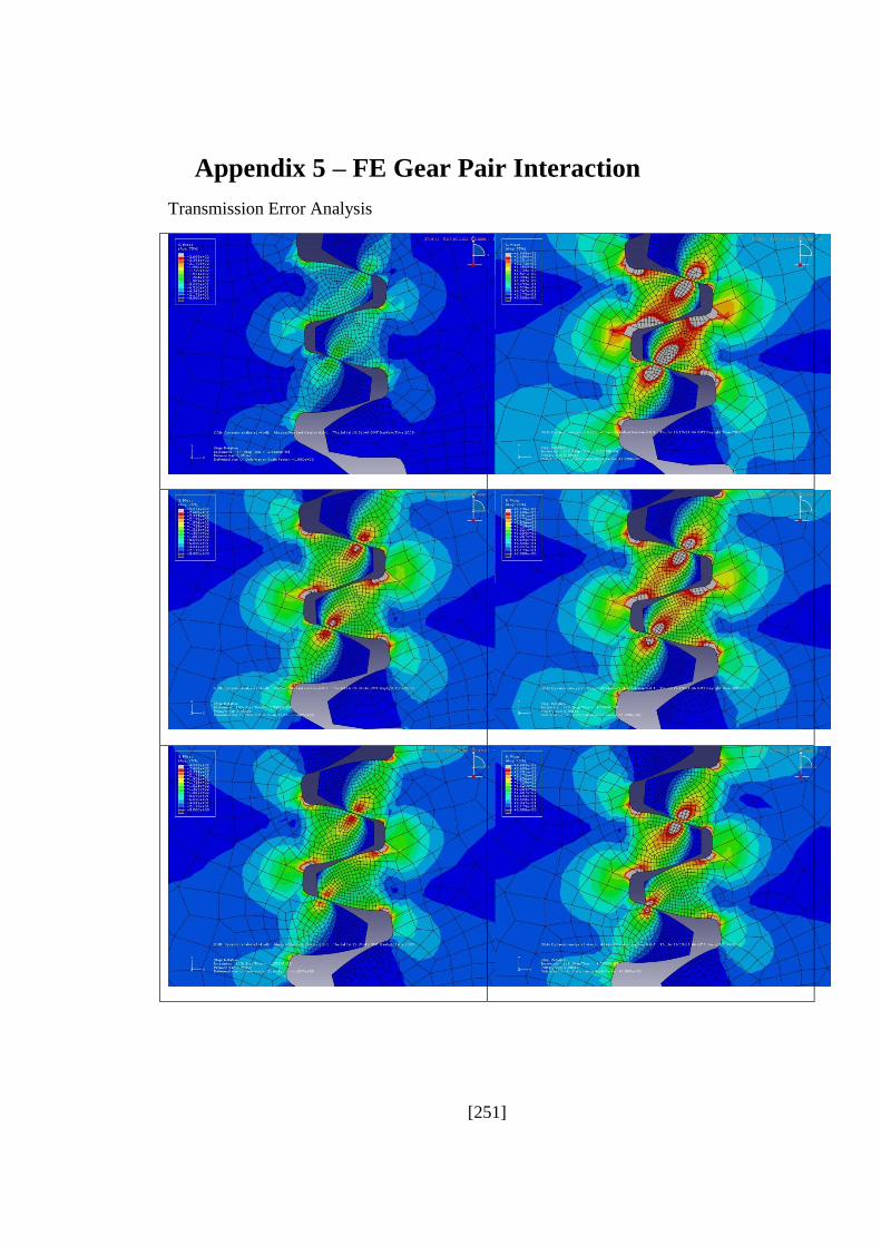
[251]
Appendix 5 – FE Gear Pair Interaction
Transmission Error Analysis
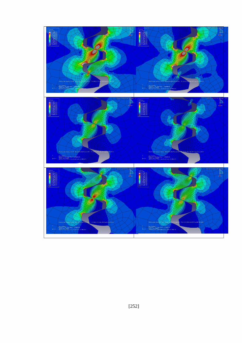
[252]

[253]
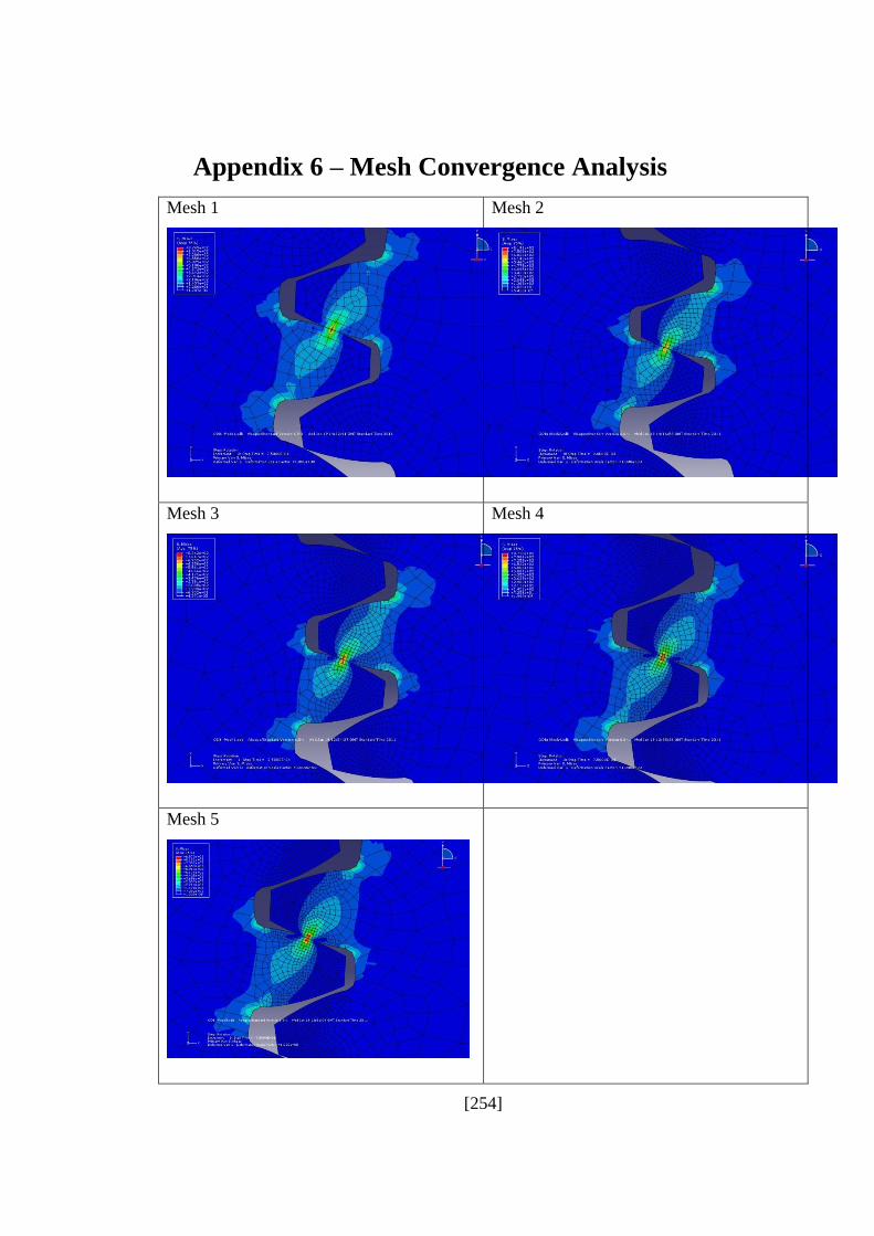
[254]
Appendix 6 – Mesh Convergence Analysis
Mesh 1
Mesh 2
Mesh 3
Mesh 4
Mesh 5

[255]