Transmission Grid Extensions for the Integration of

Variable Renewable Energies in Europe: Who Benefits

Where ?

Katrin Schabera,b,∗, Florian Steinkec, Thomas Hamachera

aInstitut fur Energiewirtschaft und Anwendungstechnik, Technical University Munich,Arcisstr. 21, 80333 Munich, Germany

bMax-Planck-Insitute for Plasmaphysics, Boltzmannstr. 2, 85748 Garching, GermanycSiemens Corporate Technology, Munich, Germany

Abstract

Variable renewable energy (VRE) generation from wind and sun is grow-

ing quickly in Europe. Already today, VRE’s power contribution is at times

close to the total demand in some regions with severe consequences for the re-

mainder of the power system. Grid extensions are necessary for the physical

integration of VRE, i.e., for power transports, but they also have important

economic consequences for all power system participants.

We employ a regional, power system model to examine the role of grid

extensions for the market effects of VRE in Europe. We derive cost-optimal

macroscopic transmission grid extensions for the projected wind and solar ca-

pacities in Europe in 2020 and characterize their effects on the power system

with high regional and technological resolution.

Without grid extensions, lower electricity prices, new price dynamics and

reduced full load hours for conventional generation technologies result in

∗k.schaber@tum.de

Preprint submitted to Energy Policy December 22, 2011

proximity to high VRE capacities. This leads to substantial changes in the

projected achievable revenues of utilities. Grid extensions partially alleviate

and redistribute these effects, mainly for the benefit of baseload and the VRE

technologies themselves.

Keywords: Renewable energy, grid integration, merit order effect

1. Introduction1

Political targets of the European Union suggest that 34% of the electric-2

ity shall be provided by renewable energies in 2020 (EU Commission, 2006).3

Major contributions will come from wind and solar energy due to their large4

potential, attractive feed-in tariffs in many countries and expected cost re-5

ductions (Edenhofer et al., 2010; IEA, 2011). Wind energy installations in6

Europe grew by 10 GW in 2009 and 2010 respectively, with additional 13 to7

19 GW expected to come online each year until 2020 (GWEC, 2011; EWEA,8

2009a). Photovoltaic installations reached 29 GW in Europe, and 17 GW in9

Germany alone in 2010 (BMU, 2011; EPIA, 2011). For 2020, EPIA sees a10

12% share of photovoltaics in European power demand as both necessarry11

and feasible for Europe to achieve its CO2 reduction goals (EPIA, 2009).12

Wind and solar energy, however, are not just another type of power plant13

that is set to replace other means of generation. They are different from14

conventional, i.e., thermal dispatchable, generation in at least three respects:15

First, generation from wind and sun fluctuates – we term them variable re-16

newable energies (VREs) in this paper. The availability of these renewable17

resources is only partly predictable, important shares of their supply remains18

stochastic. At times of low wind and sun an almost complete backup power19

2

plant park is needed, see e.g. TradeWind (2009), where the capacity credit20

of wind is only rated at 10-16% on a European level. The capacity credit of21

wind and solar energy is the dependable share of the VRE capacity, i.e., the22

amount of other generating capacity that can be removed from the system23

without reduction of the security of supply. Thus, most of today’s power24

plant park will have to stay online for a significant period of time, but with25

strongly reduced full load hours (FLH).26

The second difference is that generation from VREs is subsidized through27

feed-in tariffs in many countries. Together with extremely low variable gen-28

eration cost, this significantly changes electricity markets and their price dy-29

namics. Third, VRE generation is not spread uniformly over Europe; instead30

it is centered in regions with high meteorological potential and a supportive31

political environment, while the current power generation infrastructure is32

aligned with load centers. This generally calls for more transport capacities,33

whose realization faces several barriers, such as public acceptance and very34

long planning periods. In the mean time, above mentioned effects of VREs35

on electricity markets and conventional power plants will be experienced very36

differently in different regions of Europe.37

These qualitative arguments motivate our study. We employ a bench-38

marked, Europe-wide, power system model based on Heitmann (2005) and39

Haase (2006) to analyze the role of grid extensions for the market effects of40

the projected wind and solar capacities for 2020 in Europe. We quantify the41

regional economic effects of VREs on electricity markets and their partic-42

ipants in dependence of different grid extension levels. We investigate the43

potential of grid extension to reduce the effects of VREs to the electricity44

3

market. Economic benefits for utility owners, but also potential additional45

barriers to grid extensions are identified.46

The model is based on minimization of overall system costs. We determine47

cost-optimal transmission grid extensions. Also, schedules for conventional48

power plants, storage facilities and grid operation is determined by the model.49

Nodal marginal pricing allows us to predict electricity prices.50

Our paper proceeds as follows: In Section 2 we review related work. The51

model is described in detail in Section 3. We derive our results in Section 4,52

where we first focus on cost-optimal grid extensions and second, analyze the53

effects of VRE to the existing power system. In Section 5 we discuss our54

results before concluding in Section 6.55

2. Related Work56

The challenging properties of VREs, namely variability, uneven geograph-57

ical distribution and vanishing variable cost, spurred numerous research ef-58

forts.59

Concerning the first two issues, technical analyses have been conducted to60

identify measures how VREs can be integrated in power systems, such as61

storage, demand side management, grid extensions and more flexible power62

plants. Grid extension are thus one possible way to smoothen fluctua-63

tions and gain access to areas of high VRE potential. Giebel (2000) and64

Heide et al. (2010) quantify the statistical advantages of interlinked VRE65

generation, such as reduced need for backup and storage capacities. Tech-66

nical and geographical feasibility studies show, that a European supergrid,67

i.e., a powerful high voltage grid, facilitates visionary renewable scenarios68

4

for Europe (Biberacher, 2004; Czisch, 2005; DLR, 2006). Also, a recently69

published Roadmap (McKinsey et al., 2010) and wind integration studies70

(Greenpeace and 3E, 2008; EWEA, 2009b) judge grid extensions as necessary71

on the medium and long term to overcome excess electricity production and72

high backup capacity needs. Which lines to extend precisely has mainly been73

identified on a national level, in response to recent wind and solar capacity74

developments (for Germany: Dena (2005, 2010); Heitmann and Hamacher75

(2009); Weigt et al. (2010)).76

In addition to the temporal and geographical variability of wind and so-77

lar energy, their low level of variable costs has severe consequences on the78

electricity market: VREs and many other renewable energies have negligible79

variable costs and, therefore, rank first in the merit order: they are the cheap-80

est power supply source in terms of variable costs. Due to this cost structure81

and additionally fixed by the regulator through priority feed-in laws, the sup-82

ply curve, i.e., the sorted variable costs of all available power plants, is shifted83

whenever renewable energies contribute to the satisfaction of demand. As a84

consequence the demand curve intersects the supply curve at lower prices and85

the price level declines due to renewable supply. This is called the merit order86

effect. Sensfuss et al. (2008) show in an econometric analysis, that in 200687

the German mean wholesale electricity price was lowered by 7.8 e/MWh by88

this effect due to the integration of renewable energies. This results in a89

redistribution of economic welfare: consumer surplus increases and producer90

surplus is reduced (see also de Miera et al. (2008)). Based on the example91

of Texas, Woo et al. (2011) show that higher wind energy supply leads not92

only to lower average electricity prices, but also to higher price volatility.93

5

This volatility is sensitive to the level of wind speed, the behavior of differ-94

ent market participants (Green and Vasilakos, 2010) and the distribution of95

market power, as proven in a theoretical framework by Twomey and Neuhoff96

(2010). Based on a probabilistic power generation model MacCormack et al.97

(2010) point out, that opposite to the sinking electricity price, the total98

costs of the power supply rises with increasing wind contribution. Measures99

to alleviate the effects of VREs to the electricity price are investigated by100

Jacobsen and Zvingilaite (2010) for Denmark focusing on storage, demand101

side management and real time pricing. Leuthold et al. (2009) demonstrate,102

that the reduction of electricity prices due to wind integration can be di-103

minished with grid extensions in Europe. They find, that European grid104

extensions lead to an overall welfare gain.105

In this study we determine cost-optimal grid extensions for Europe in106

2020 to integrate VREs and investigate the role of the grid for electricity107

markets and their participants. The studies mentioned above showed the108

necessity of grid extensions and the effects of VREs to the electricity prices in109

general. We apply a regionally resolved power system model based on linear110

optimization which includes electricity transport between regions and allows111

to determine necessary grid extensions. Our methodology allows to draw112

conclusions for each region and generation technology in detail. We quantify113

changes in power producer revenue due to VREs as well as the effect of grid114

extensions for each generation technology type in order to identify possible115

proponents and opponents to grid extensions for VREs in Europe.116

6

3. The Model117

3.1. Model Formulation118

AB

BGBH−Co

CZ

Ch

D−EON−M

D−EON−N

D−EON−SD−EnBW

D−RWE

D−VET

DK−ODK−W

ES−NW

ES−OES−S

F−NOF−NW

F−SOF−SW

FIN−N

FIN−S

GB−N

GB−S

GR

HI−N

I−SI−SarI−Siz

IRLIRL−NI

Kro

Lux

N−M

N−N

N−S

NL

P−M

P−N

P−S

PL

Ro

S−M

S−N

S−S

SK

SLO

SRB

GW0 − 11 − 22 − 33 − 44 − 55 − 66 − 77 − 88 − 99 − 10

Figure 1: European model regions with aggregated ENTSO-E transmission grid

The applied methodology in this study is a power system model based on119

linear optimization of overall costs from a social planner perspective. The120

model, called URBS-EU, is an extension of the German energy system model121

URBS-D (Heitmann, 2005; Haase, 2006). It divides Europe into 83 regions,122

50 of which correspond to the major Transmission System Operator (TSO)123

regions in the European Network of Transmission System Operators for Elec-124

tricity (ENTSO-E) grid and 33 to specific offshore regions (see Figure 1). The125

temporal resolution is hourly. Thanks to this high level of detail, the model126

is appropriate to analyze variable resources, such as wind and solar energy.127

The structure of the overall system costs subject to minimization is128

COST =∑x,i

{κIiCNi(x) + κF

i Ci(x) +∑t

κV ari Eout

i (x, t)}. (1)

7

They include the annuity of investment costs κIi , fix, capacity-dependent Op-129

eration and Maintenance costs κFi as well as the variable costs κV ar

i for power130

plant, storage and transmission technologies. The costs per technology i are131

given in Table 1. Ci(x) is the total capacity, CNi(x) the capacity additions132

per technology i and region x and Eouti (x, t) is the power production per re-133

gion, technology and time-step t. Through optimization of the total system134

costs, power plant dispatch, Eouti (x, t), per region and technology, is deter-135

mined. On demand, the model also computes cost-optimal extensions of the136

power plant, storage and transmission infrastructure, based on the annuity137

of investment costs. This is achieved by using CNi(x) as free variable, in138

addition to Eouti (x, t).139

The linear optimization is subject to restrictions which describe the proper-140

ties of the power supply system. A complete list of the equations defining141

the model URBS-EU is given in Appendix A.1. The most important con-142

straint, is that electricity demand d(x, t) has to be satisfied in each region143

and time-step:144

∑i

Eouti (x, t)− Ein

Transmission(x, t)− EinStorage(x, t) ≥ d(x, t). (2)

In the energy balance (equation 2), the electricity export (EinTransmission(x, t))145

and feed-in to storage (EinStorage(x, t)) have to be taken into account. The146

dual solution to this equation gives the marginal costs of electricity genera-147

tion. Assuming a well functioning electricity market, the marginal costs are a148

good indicator of the wholesale electricity prices (Borchert et al., 2006). The149

marginal costs are determined by the variable costs of generation, storage150

8

and transmission. Transmission and storage losses indirectly translate into151

increased marginal and total costs, as they lead to higher demand for power152

generation (see equation 2). In our model, excess production is possible. To153

ensure stable operation of the power system, generation that exceeds demand154

has to be discarded. If no excess production was allowed for, negative price155

would occur. So in our model, negative prices are not taken into account.156

This approximation is justifiable, as in reality negative prices occurred only157

in very few hours in the past (EEX, 2009). Moreover, negative prices will158

most likely be compensated by market participants, who create additional159

demand such as thermal storage for example and take advantage of the neg-160

ative price events.161

Further restrictions to the cost-optimization are maximum generation con-162

straints for each generation and storage technology and region:163

Eouti (x, t) ≤ afi · Ci(x). (3)

Reduced average availability of power plants due to planned and unplanned164

outages are included with an availability factor afi. Similar upper bounds for165

storage and transmission capacity are included in the model and storage and166

transmission losses as listed in Table 1 are taken into account. Hourly values167

of the capacity factor cfi(x, t) for VREs serve as constraints to the operation168

level of variable renewable technologies. The time dependent capacity factor169

is deduced from meteorological data (see Subsection 3.2 and Heide et al.170

(2010))171

Eouti (x, t) = cfi(x, t) · afi · Ci(x) , ∀i ∈ V RE cfi(x, t) ∈ [0, 1] (4)

9

where V RE includes wind on- and offshore, solar PV and also run-off river172

hydro power plants.173

Technology specific ramping constraints, i.e., a speed-restriction for changes174

in electricity generation, are included in the model.175

|Eouti (x, t)− Eout

i (x, t− 1)| ≤ pci · Ci(x) (5)

The maximal power change pci per technology is listed in Table 1. Ramping176

constraints are crucial to model power plant dispatch with a linear opti-177

mization model. Commonly more realistic results can be achieved with unit178

commitment models, who require Mixed Integer Programming and are com-179

putationally expensive. Aboumahboub (2011, Ch. 2.4) shows that through180

the inclusion of ramping constraints in linear models, the results from linear181

optimization and a unit commitment model converge. Ramp-up costs are182

not included, but the above restriction leads to an increase in total costs,183

as it constrains the cost-optimal dispatch of power plants and can lead to184

higher power generation.185

We perform a simplified simulation of electricity transmission between186

regions. Kirchhoff’s first law, the conservation of currents in each node of an187

electricity network, is respected in our model, while the second, the voltage188

law, is not included. Electricity transmission is thus modeled as a transport189

problem, neglecting effects of load flows (see Appendix A.1). The approxi-190

mation of electricity transmission with a transport model allows to keep the191

optimization problem linear and to optimize grid extensions and power plant192

additions and operation simultaneously.193

The model is formulated and optimized using the General Algebraic Mod-194

10

eling System (GAMS) software package. The optimization is performed for195

six representative weeks of each year of available meteorological data (2000-196

2007). The selected weeks include the minimal and maximal residual elec-197

tricity demand, are distributed uniformly across seasons and have minimal198

deviation from the respective annual full load hours (FLH) of wind and solar199

(less than 3%). Model results are presented as aggregation over the eight200

years of available data, where energy-related parameters are averaged over201

the eight years and for capacities, the maximal values are presented.202

3.2. Model Data203

The cost assumptions and the technical parameters, shown in Table 1, are204

based on scientific studies (IEA, 2010b; McKinsey et al., 2010; PWC et al.,205

2010) and industry expert evaluations. Technical parameters, such as con-206

version and transmission and storage losses ηi, ramping constraints and re-207

stricted availability, are included also listed in Table 1. The ramping con-208

straints includes the technical ramping restrictions for each individual power209

plant, but also the inertia of the aggregated generation capacity per genera-210

tion technology in each model region. Here some power plants might be shut211

of and have to respect minimal time of non-use or cold start restrictions. As212

a results, aggregated ramps are slower than individual ones.213

To model wind and solar energy supply, we use an eight years dataset214

of highly resolved weather data based on the Heide et al. (2010). Hourly215

capacity factors for wind and solar energy have been determined based on an216

eight years dataset (2000-2007) of highly resolved (50 km) reanalysis data.217

The aggregation of capacity factors from the 50 km cells to the 83 European218

model regions is based on a wind and solar capacity distribution across the219

11

Technology Inv.Costs

FixO&MCosts

Var.Cost

η afi pci

e/kWel e/kWel e/MWhel % % %/h

Bioenergy 2500 50 18 38% 40% 25%Coal 1400 35 21 46% 80% 22%Gas GT 400 18 68 38% 100% 100%Gas CCGT 650 18 44 60% 90% 22%Geothermal 2800 80 4 45% 100% 25%Lignite 2300 40 13 43% 80% 14%Oil GT 800 18 126 35% 100% 100%Oil CCGT 900 18 89 50% 90% 22%Nuclear 3000 65 12 33% 80% 8%Hydro run of river 1400 20 5 75% 100% 100%Hydro storage 1539 20 - 85% 100% 100%HV lines ,e/MWkm 400 0.7 - 96%/1000km 100% 100%HV cable ,e/MWkm 2500 0.7 - 96%/1000km 100% 100%

Table 1: Investment, fixed operation & maintenance and total variable costs. The variablecosts include fuel costs and variable operation & maintenance costs, but not the carboncosts. For the computation of the annuity of investment, a weighted average cost of capital(WACC) of 7% is assumed. CCGT stands for Combined Cyle Gas Turbine and GT forGas Turbine.

50 km cells determined in accordance to planned projects, national policies220

and actual potential. Most recent wind turbine generators and solar pho-221

tovoltaic cells (PV) are assumed. The hourly load curve for the years 2000222

- 2007 stems from the European Transmission System Operator ENTSO-E223

(ENTSO-E, 2010). We select six representative weeks for each of the eight224

years database and model 48 (six times eight) weeks in total.225

The existing grid infrastructure is obtained from freely available data on226

the European high voltage (HV, 220kV and 380kV) electricity grid (ENTSO-E,227

2010). A Geographic Information System is applied to digitalize the map of228

the transmission grid and intersect it with the model regions. HV transmis-229

12

sion lines are commonly operated at their natural load level, where no voltage230

drop occurs. Therefore we compute the total transmission capacity between231

model regions based on the natural load of all HV lines linking two model232

regions. In dependence on the voltage level, the natural load for each HV233

line is calculated. The aggregation of all HV lines between two model regions234

results in the total transmission capacity. Results are shown in Figure 1.235

We built a geo-referenced power plant database to determine the ac-236

tual generation capacities per model region. The database combines the237

UDI power plant database (Platts, 2009) and a second data base including238

energy production, emission and geographic location of each power plant239

(Wheeler and Ummel, 2008). Coupling these two datasets on power plant240

level provides a powerful and exhaustive geo-referenced database for Europe.241

The future power plant fleet is extrapolated with technology specific lifetimes242

(IEA, 2010b; Oko-Institut, 2008).243

In all scenarios in this paper, we assume that the demand remains the244

same as in 2007. Studies and a constant trend in the last years support this245

assumption (McKinsey et al., 2010; ENTSO-E, 2009).246

We benchmark our model against historical data. The validation shows,247

that the model reproduces the current European electricity system in ade-248

quate accuracy. This is presented in detail in Appendix A.2.249

3.3. Scenario Setup250

We apply the model to study the effects of increasing shares of wind and251

solar energy in Europe in 2020 and the role of transmission grid extensions.252

As mentioned above, power plant dispatch, but also infrastructure ex-253

tension can be determined by the optimization. In this study, VRE ca-254

13

pacity additions for 2020 are exogenous to the model and drawn from the255

National Renewable Energy Action Plans of the European Member States256

(Beurskens and Hekkenberg, 2011). Regional distributions within countries257

are based on previous studies, political commitments and planned projects258

(Bofinger et al., 2008; TradeWind, 2009; EWEA, 2008) and shown in Fig-259

ure 2. The total planned wind capacity of 218 GW is similar to previous260

studies assumptions: for wind on- and offshore power a total European ca-261

pacity of 180 GW in 2020 was assumed by EWEA (2008), 150 GW by the262

IEA, 128-238 GW by OffshoreGrid (2010) and 280 GW by GWEC (2011).263

For solar PV, 92 GW are projected for 2020. The National Renewable Ac-264

tion Plans exceed the projection of 45 GW Solar PV capacity in 2020 by IEA265

(2010c), but are roughly in line with the projection of EPIA (2011) of more266

than 60 GW in 2015.267

By 2020, some of the existing conventional power plants will be retired and268

the technology mix of the necessary power plant additions (CNi(x) ∀ i /∈269

{V RE, Storage}) are determined by the cost-optimization for each scenario270

for the scenario year 2020. For some technologies, such as nuclear power271

and other renewable power (hydro, bio- and geoenergy), political and geo-272

graphical limits are taken into account (see Table 2). The model allows to273

compute cost-optimal transmission grid extensions between model regions.274

In the scenarios we study different levels of grid extensions. Addition of stor-275

age capacity, is not allowed in this study focusing on grid extensions only.276

We assume, that current storage capacities are installed in 2020, reflecting277

the limited geographic potential for additional pumped hydro storage capac-278

ity. Finally, the power plant dispatch and usage of the transmission grid and279

14

existing storage capacities (Eouti (x, t)) results from the optimization and its280

boundary conditions, in particular equation 2, 3 and 4.281

Input parameter Base No Grid New Lines New Cables

VRE capacities current ca-pacities

projected capacities for 2020(Beurskens and Hekkenberg, 2011)

Installed nonVRE capacities

projected capacities for 2020 (retirements are taken intoaccount), current hydro storage and run-of-river capaci-ties (Platts, 2009)

Limits for ca-pacity additions

capacity addition for nuclear, geothermal and bioenergyare limited to maximum between 2020 extrapolations andcurrent capacities, no VRE additions allowed, infinite forall other generation technology

HV transmis-sion grid

currentENTSO-Egrid

currentENTSO-Egrid anddirect con-nectionsof offshorewind toshore

overheadline ex-tensionsbetweenneighborspossible.Sea-cablesallowed onselectedconnections

cable ex-tensionsbetweenneighborspossible.Sea-cablesallowed onselectedconnections

Carbon price 30 e/t 30 e/t 30 e/t 30 e/t

Table 2: Definition of scenarios

Table 2 lists the characteristics of the four scenarios. The Base scenario282

serves as comparison for the VRE scenarios. It mimics the power supply283

system by 2020 without the projected VRE capacity additions. For the VRE284

scenarios we investigate three levels of grid extensions: today’s network (No285

Grid) and two cases of cost-optimal grid extensions: in the New Lines sce-286

nario new overhead lines and offshore cables are allowed, in the New Cables287

scenarios only cable extensions on- and offshore are possible. Cables are288

about six times more expensive than overhead lines (see Table 1). The sec-289

15

ond case therefore results in less grid extensions. The New Cables scenario290

thus allows to identify the most important grid extension and furthermore291

represents one possible technical response to public resistance towards new292

overhead transmission lines.293

(a) Wind Onshore(152 GW)

(b) Wind Offshore(66 GW)

05

1015

20

(c) Solar Photovoltaics(92 GW)

Figure 2: Capacities of Variable Renewable Energies for 2020 in GW (seeBeurskens and Hekkenberg (2011)). Total European capacity per VRE technology is in-dicated in brackets.

4. Results: European electricity supply in 2020294

We apply the model URBS-EU to analyze grid extensions as a measure295

to address economic effects of high VRE penetration in Europe. In a first296

step we present cost-optimal high voltage transmission grid extensions for297

Europe in 2020, then turn to the impacts of the planned VRE capacities to298

the existing power plants and finally study prices and revenues per generation299

technology and region.300

16

4.1. The Cost-Optimal Grid301

GW 0.0 − 2.5 2.5 − 5.0 5.0 − 7.5 7.5 − 10.010.0 − 12.512.5 − 15.015.0 − 17.517.5 − 20.020.0 − 22.5

(a) New Lines

GW 0.0 − 2.5 2.5 − 5.0 5.0 − 7.5 7.5 − 10.010.0 − 12.512.5 − 15.015.0 − 17.517.5 − 20.020.0 − 22.5

(b) New Cables

Figure 3: Cost optimal grid extensions

The cost-optimal grid extensions in the New Lines and New Cables sce-302

nario are depicted in Figure 3. Large transmission capacities result from303

the optimization model. The total the grid capacity increases by almost304

60% in the New Lines scenario and by more than 20% in the New Cables305

scenario compared to the current ENTSO-E grid capacity and length (in306

MWkm). This is plausible from an economic point of view, since new lines307

are relatively cheap compared to the additional use of fossil fuel (see Table 1).308

Overhead lines are less expensive than cables (see Table 1) and therefore, less309

grid extensions result in the New Cables scenario. The grid extensions are310

driven by the VRE capacity addition, but also bear benefits for conventional311

power plants.312

17

Germany, France and BeNeLux1 act as transit countries. In north-western313

France, northern Germany and Great-Britain substantial grid extensions are314

cost-effective in both scenarios to integrate the large wind capacities in these315

areas. Large new grid capacities result for the Spanish-French connection,316

but only little additions on the Iberian peninsula occur. Italy, having a317

rather weak electricity grid today, profits from a cost-effective enforcement318

of its connection to France. Offshore grid extensions are mainly located in319

the Northern and Baltic Sea, in proximity to important on- and offshore320

wind capacities. In the New Lines scenario the majority of grid extensions321

are onshore as lines are cheaper than cables, while in the New Cables sce-322

nario larger shares of the grid extensions are offshore cables. We assumed323

identical costs for on- and offshore cables. In BeNeLux and Italy for instance,324

offshore grid extensions are more cost-effective than onshore cable extensions325

in the New Cables scenario. If overhead lines can be built, the bulk power326

transmission takes place onshore (New Lines).327

We find that an offshore grid in the Northern sea is cost-effective, in328

consistency with other studies. On- and offshore grid extensions for wind329

integration proposed in TradeWind (2009) and Kerner (2007) show the same330

corridors as the ones identified in this study. EWEA (2009b) focuses on Eu-331

ropean offshore wind parks and proposes a powerful interconnected offshore332

network in the Northern and Baltic Sea. The proposed capacities for 2020333

and 2030 by the EWEA are in line with our results.334

18

Bas

e

No

Grid

New

Lin

es

New

Cab

les

GW

0

200

400

600

800

1000

1200

(a) Capacities

Bas

e

No

Grid

New

Lin

es

New

Cab

les

TWh

0

1000

2000

3000

4000

(b) Total Energy Production ●

●

●

●

●

●

●

●

●

●

●

●

●

●

●

●

●

●

●

●

Pumped StorageSolar CSPSolar PVWind OffshoreWind OnshoreGas GTOil GTGas CCGTOil CCGTGeoenergyCoalBioenergyLigniteNuclearHydro

Figure 4: Power plant capacities and energy production in 2020 for all scenarios. Shadedareas represent capacity additions.

4.2. Power Plants335

Figure 4 presents the model results for power plant capacities and energy336

generation in Europe.337

To the 690 GW of the power plants that will still be on line in 2020, the338

optimization model adds about 115 GW new capacity in the Base scenario339

to replace retired power plants and those shut down for political reasons,340

such as the phase-out of nuclear power in Germany. Capacity additions are341

represented by shaded areas in Figure 4(a). The additional 234 GW new342

VRE capacity lead to a slight reduction of conventional capacity additions343

in the No Grid scenario, where 100 GW non-VRE capacity is added. This344

corresponds to a capacity credit of the VRE technologies of 4%. With grid345

extension less new thermal capacity is needed: about 80 GW is added in the346

New Lines and about 90 GW in the New Cables scenario. The capacity credit347

1including Belgium, the Netherlands and Luxembourg

19

increases to 14% and 9% respectively. In all scenarios, nuclear and gas power348

plants are the only technologies, where new capacities are added. Compared349

with the European peak load of 619 GW, the conventional installations are,350

however, still able to provide full backup for the VREs in all scenarios.351

Figure 4(b) shows the model’s outputs regarding the energy mix. Since352

the VREs’ share in total electricity production increases from 5% to 21%353

through the VRE capacity additions, the conventional power plants’ output354

is significantly reduced, while conventional capacity remains close to current355

capacity. The averaged full load hours (FLHs) over all thermal generation356

types (Coal, Lignite, Gas, Oil, Nuclear and Bio- and Geoenergy) decrease357

by 9% in No Grid case.With grid extensions (New Lines) the total average358

reduction in FLH for thermal generation types amounts 5% and baseload359

power, mainly nuclear, replaces peaking technologies such as gas, as can be360

seen in Figure 4(b).361

The reduction in power plant usage is most severe in regions with high VRE362

deployment and will create severe pressure for the conventional power plant363

operators. In regions with high VRE capacity, the FLHs of base load power364

plants such as nuclear and coal generation units decline sharply, if no grid365

extensions are realized, because they have to adapt to VRE supply (see366

Figure 5). With an extended, cost optimal grid, more traditional usage of367

the power plants is possible: baseload power is used more continuously, while368

the mid and peak load power plants also in the neighboring regions help to369

balance the VRE fluctuations. These technologies in turn supply less energy370

in total.371

20

No Grid New LinesNuclear

2000

3000

4000

5000

6000

7000

8000

Coal

2000

3000

4000

5000

6000

7000

8000

Gas

CCGT

020

0040

0060

0080

00

Figure 5: Full Load Hours of nuclear, coal and gas power plants for the No Grid and NewLines scenario

One of the most affected regions by new VRE capacities is north-western372

Germany. Here, 18 GW offshore wind capacity is projected for 2020, 4 GW373

of solar PV and 6 GW of wind onshore capacity (see Figure 2). Many im-374

portant effects of the VRE integration for the power plants can be studied375

21

in detail from Figure 6, where the computed energy mix and the resulting376

energy prices for the North-Western German region D-EON-N are shown for377

one of the eight modeled meteorological years.378

In the Base scenario, the base load is covered by nuclear and coal power379

plants, gas power plants and also electricity import from neighboring regions380

provide the mid and peak load. The region exports electricity, as can be read381

off from the difference between the yellow line, the electricity demand within382

the region, and the orange total demand line where export and storage charg-383

ing is included. In the Base scenario, the current onshore wind capacity of384

5.3 GW is installed.385

In the scenarios No Grid and New Lines, large amounts of additional wind386

energy from a dedicated offshore region are imported into the considered387

region, shown as gray areas in Figure 6 (b) and (c). This results in drastic388

changes in the power plant dispatch, if no grid extensions are carried out (No389

Grid). In windy hours, wind energy replaces power from peak, middle and390

also base load power plants. Even nuclear power has to shut down several391

times. With grid extensions (New Lines), the base load power plants can392

be used in a more traditional way. The burden of balancing the fluctuating393

wind energy is then shared between all peak and mid load power plants in394

the linked neighboring regions.395

Also the capacity additions alter slightly across scenarios: in the Base case396

slightly more new Gas CCGT capacity (1.3 GW) is installed.397

398

22

Capacities Energy Mix Electricity price

HydroNuclearLigniteBioenergyCoal

Gas CCGTGas GTWind OnshoreSolar PV

Pumped storageImportDemandDemand + Export

(a) Base

(b) No Grid

(c) New Lines

Figure 6: Energy mix in north western Germany (D-EON-N ) and electricity price forselected weeks in 2020 (meteorological data from 2003).

4.3. Electricity prices and revenues399

Not only power plant dispatch changes considerably with VRE capacity,400

also the electricity prices are strongly influenced.401

This can be seen for north western Germany in Figure 6. Power supply from402

VRE strongly influences electricity prices. Their variable costs are close to403

zero and thus, wind power enters at the first position in the merit order of404

power plants. Whenever wind and solar energy supply is sufficient to satisfy405

the demand, the price drops to zero and through the merit order effect, the406

electricity price in regions with high VRE capacity is lowered. As mentioned407

in Section 3, negative prices are not taken into account.408

23

Figure 7 shows the average electricity price for the four scenarios. The av-409

erage electricity price in Europe is 62 e/MWh in the Base scenario. In the410

No Grid it drops to 52 e/MWh, 17% lower than the basecase. With grid411

extensions the average price recovers to 55 e/MWh and 53 e/MWh with412

new lines or cables respectively. As can be seen from the maps, regions413

with high VRE capacity are most affected by the reductions in electricity414

price. In north-western Germany, the average price drops from 65 e/MWh415

to 50 e/MWh with 2020 VRE capacity additions and no grid extensions (see416

also Figure 6). Generally speaking, the standard deviation of electricity price417

across regions increases with increasing VRE capacity. In the Base case the418

standard deviation of elecricity prices across the European regions amounts419

5 e/MWh. It increases to 8 e/MWh and can be lowered with grid extensions420

to 3 and 6 e/MWh respectively. Grid extensions lead to a homogenization421

of the electricity prices.422

24

Base No Grid

2030

4050

60

New Lines New Cables

2030

4050

60

Figure 7: Average electricity price (e/MWhel)

Furthermore, the dynamics of the prices changes. While in the current423

system and in the Base case, the electricity price is mainly determined by424

the load (see Figure 6), the average correlation between load and prices drops425

to around 25% in the 2020 VRE scenarios from 75% today. In turn, gener-426

ation from wind turbines plays an increasingly important role for electricity427

prices. In regions with high VRE capacity strong anticorrelation between428

wind generation and electricity prices can be observed, see Table 3. Solar429

power generation is generally smaller and also closer to the load. Therefore,430

its effects to the electricity price are not yet as pronounced. Grid extensions431

reduce the anticorrelation between wind and price. With grid extensions, the432

25

anticorrelation is reduced by about 50% in affected regions (see Table 3).433

Correlationprice and wind

Spain NW Scotland Germany NW

No Grid -61% -50% -32%New Lines -28% -20% -16%New Cables -58% -36% -17%Wind capacity(GW)

18 11 23

Table 3: Correlation between electricity price and generation from wind energy in selectedregions. The last row lists the total on- and offshore wind capacity in the regions.

The changes in electricity prices and FLHs affect the revenues of the util-434

ities. Figure 8 shows the average annual revenue per installed MW for each435

generation technology. All technologies are affected and achieve lower rev-436

enues. Note, that Figure 8 shows the average revenues per technology. New437

power plants will be used more frequently, due to higher efficiency and result-438

ing lower variable costs. They may thus achieve higher revenues. However,439

for some peaking technologies, the benefit is small and balancing markets440

have to be used as well. Stagnant investment in new power plants before the441

economic crisis reflects the difficulties at the market (Dena, 2008). Without442

grid extensions for the new VRE capacity (No Grid), the standard deviation443

of the revenue across regions increases due to the inhomogeneous distribution444

of VRE capacities in 2020. The profitability of conventional power plants will445

be strongly influenced by the amount of VRE capacity close by.446

Network improvements lead to more uniform prices in time and space. They447

reduce the standard deviation of the revenues across the regions significantly.448

VREs are affected very positively by grid extensions since fewer low price sit-449

uations occur. As large VRE generation mainly causes the low prices, these450

26

technologies can hardly earn important revenue in the current market struc-451

ture (Neuhoff, 2005). Grid extensions smoothen the electricity price. As452

a result, less low price events occur and the revenues for VRE increases.453

Baseload power plants such as nuclear, coal and lignite also benefit sub-454

stantially from grid extensions. The average revenues reach current levels455

if cost-optimal overhead transmission extensions are realized. For mid and456

peak-load power plants, the economic situation remains difficult even with457

large grid extensions, due to important FLH reductions.458

459

050

100150200250300350400450500550

Nuclear Lignite Coal Bioenergy Gas CCGT Gas GT Wind Onshore Solar PV

Annu

alrevenu

e(€/kW/yr)

Base

No Grid

New Cables

New Lines

Standard deviationMin. and Max.

Baseload Peakload VRE

Figure 8: Revenues per generation technology for the four scenarios. Standard deviationand minimal and maximal values across the model regions are indicated with the blacklines.

Figure 9 shows the change in revenue due to VRE additions by country.460

Regions with largest additions are most affected, as for example Germany,461

Spain, France and Great Britain, where the revenues for nuclear power are462

reduced by up to 25%. Looking in more detail, in north-western France and463

in Scotland, revenue for nuclear reach is reduced by more than 50% from the464

Base to the No Grid scenario. As pointed out before, VREs are most af-465

fected if they participated in the electricity market directly. For Gas CCGT466

27

power plants, a mid and peak load technology, grid extensions show only467

little effect and the revenue remains low. In importing regions, such as Italy,468

grid extensions can even lead to an additional decrease revenue.469

470

In general, transmission grid extensions reduce the future revenue reduc-471

tion from VRE and distribute the economic surpluses evenly across intercon-472

nected regions.473

Nuclear No Grid New Lines New Cables Windny / 70 D 70 Germany 13% 8% 10% D 7031 ES 31 Spain 17% 7% 16% ES 31ritain /GB 27 Great Britain 12% 12% 14% GB 27/ 27 F 27 France 26% 2% 9% F 27ands / NL 10 Netherlands 13% 10% 12% I 17/ 6 PL 6 Poland 9% 6% 8% NL 10

m / 5 B 5 Belgium 12% 9% 11% GR 9a / 4 Ro 4 Romania 13% 3% 10% PL 6/ 4 S 4 Sweden 5% 2% 2% P 5/ 3 FIN 3 Finland 8% 2% 6% B 5epubliCZ 2 Czech Republi 6% 6% 6% N 4and / Ch 1 Switzerland 6% 7% 6% IRL 4y / 1 H 1 Hungary 8% 6% 7% S 4a / 1 SK 1 Slovakia 8% 6% 7% CZ 2a / 0 SLO 0 Slovenia 7% 8% 7% Kro 2

A 2DK 2Ch 1H 1SK 1Lux 0

2 3 4 2 3 4 2Nuclear Wind Gas CCGT2020 No Grid 2020 New Line2020 New Cab2020 No Grid 2020 New Line2020 New Cab2020 No Grid

70 Germany 0.12548597 0.08142776 0.09851086 0.22980899 0.17117347 0.19925338 #N/A31 Spain 0.17263633 0.06903314 0.15590318 0.25146442 0.05965175 0.21512287 #N/A27 Great Britain 0.1158804 0.11502062 0.1360225 0.52681672 0.19911708 0.40233677 #N/A27 France 0.25659512 0.02318344 0.08595423 0.46616959 0.04503543 0.19681169 #N/A17 Italy 0.08231544 0.10622756 0.09682593 #N/A10 Netherlands 0.13201464 0.09770468 0.11853564 0.24187959 0.17277667 0.21965865 #N/A9 Greece 0.13185422 0.15197234 0.14361156 #N/A6 Poland 0.08964683 0.0630803 0.08278812 0.12301626 0.09196664 0.11621908 #N/A5 Portugal 0.32982771 0.19672964 0.29985512 #N/A5 Belgium 0.11980463 0.08871144 0.10717862 0.22135466 0.16264317 0.20295756 #N/A4 Norway 0.22063563 0.08115764 0.20505848 #N/A4 Ireland 0.71262136 0.14148516 0.32098869 #N/A4 Sweden 0.05288244 0.0169238 0.02120293 0.17764922 0.10781789 0.16070374 #N/A3 Finland 0 07700818 0 02022819 0 06443141 #N/A

30%25%20%15%10%5%0%5%

10%

Germ

any/7

0

Spain/3

1

GreatB

ritain/2

7

France

/27

Italy/1

7

Nethe

rland

s/10

Greece

/9

Poland

/6

Portugal/5

Belgium

/5

Norway

/4

Ireland

/4

Swed

en/4

CzechRe

public/2

Croatia

/2

Austria

/2

Denm

ark/2

Switzerland

/1

Hungary/1

Slovakia/1

Luxembo

urg/0

Change

inRe

venu

edu

eto

VRE

Nuclear

80%70%60%50%40%30%20%10%0%

10%

Germ

any/7

0

Spain/3

1

GreatB

ritain/2

7

France

/27

Italy/1

7

Nethe

rland

s/10

Greece

/9

Poland

/6

Portugal/5

Belgium

/5

Norway

/4

Ireland

/4

Swed

en/4

CzechRe

public/2

Croatia

/2

Austria

/2

Denm

ark/2

Switzerland

/1

Hungary/1

Slovakia/1

Luxembo

urg/0

Change

inRe

venu

edu

eto

VRE

Wind

80%70%60%50%40%30%20%10%0%

10%

Germ

any/7

0

Spain/3

1

GreatB

ritain/2

7

France

/27

Italy/1

7

Nethe

rland

s/10

Greece

/9

Poland

/6

Portugal/5

Belgium

/5

Norway

/4

Ireland

/4

Swed

en/4

CzechRe

public/2

Croatia

/2

Austria

/2

Denm

ark/2

Switzerland

/1

Hungary/1

Slovakia/1

Luxembo

urg/0

Change

inRe

venu

edu

eto

VRE

Gas CCGT

No Grid New Cables New Lines

Figure 9: Relative change in revenue with VRE additions compared to Base. The countriesare plotted in decreasing order of VRE capacity additions. After the country names VREadditions until 2020 are indicated in GW.

28

5. Discussion474

In this study we apply a regionally-resolved, power system model to an-475

alyze the role of grid extensions for the interaction of wind and solar energy476

with electricity markets in Europe. Our results show, that the expected VRE477

extensions for 2020 have significant impact on electricity markets and their478

participants. Wholesale electricity prices decrease on average, their variance479

in time and space increases, and they are dynamically correlated with VRE480

supply rather than with power demand. Transmission grid extension can481

help to reduce the market effects of VREs, and moreover creates benefits for482

other generation technologies.483

484

We investigate two levels of grid extensions, where in a first stage we485

allow overhead grid extensions between all neighboring regions. The cost-486

optimal grid additions amount 60% of current grid capacity and length. In487

a second scenarios, taking into account public acceptance and political chal-488

lenges, only cable additions are allowed, and a 20% increase in grid capacity489

results.490

Regardless of the level of grid extensions, the VRE additions projected for491

2020 have severe consequences for all other power plant types. Due to the492

limited capacity credit of wind and solar power, conventional generation ca-493

pacity is hardly reduced as compared to current level, while the share of VRE494

in total electricity generation increases from 5% to 21%. This results in a495

reduction of FLHs for all conventional generation technologies.496

Without grid extensions, very high FLH reductions occur in proximity to im-497

portant VRE capacities. Through the merit order effect, VREs furthermore498

29

lower the average simulated electricity prices by more than 15% in 2020.499

Utility owners will face drastic FLH reduction and higher wearout of their500

turbines due to increased ramping if wind or solar capacity is built close by.501

The oversupply of electricity in regions with large VRE capacity and insuffi-502

cient transmission capacity furthermore lowers the electricity price drastically503

in these regions. In the current market structure, conventional power plants504

will therefore face serious economic challenges. In regions with large VRE505

capacities, the reduction in revenue for conventional base, mid and peak load506

power plants can reach 60%. The average revenue for baseload technologies507

is reduced by about 15%, for peakload by 30%. VRE capacities in 2020 thus508

create major inequalities in Europe, if no grid capacity additions are carried509

out simultaneously.510

Our results concerning the electricity price reduction are on the conservative511

side, as we do not take into account negative prices in our model. If nega-512

tive prices were included, the average prices would be lower. In periods and513

regions with negative prices it would furthermore become beneficial to shut514

down power plants, even VRE technologies.515

516

With grid extensions, the average utilization of baseload technologies is517

raised again and less ramping of baseload technologies is necessary, as the518

balancing of VRE supply is shared between more flexible power plants in519

the interconnected regions. Furthermore, the burden of reduced revenues for520

conventional power plants due to VRE extensions is distributed more evenly521

among all regions. Both levels of simulated grid extensions boost the revenue522

for baseload and VRE technologies. Revenues close to pre-VRE levels can523

30

however only be attained with a substantial grid growth of 60%. For mid- and524

peakload power plants, average revenues remain low. For VRE technologies525

themselves the anti-correlation between electricity prices and VRE genera-526

tion creates a large incentive for grid extensions, if market participation of527

these technologies is desired. Grid extensions reduce the anti-correlation of528

prices with VRE generation and thus raises the revenue for VRE technolo-529

gies.530

As a result, grid extensions are economically very advantageous for baseload531

and VRE utility owners – a rather unlike pair. In the overall picture, a pow-532

erful international transmission grid thus bears many advantages. It lowers533

overall system costs (we derive grid extensions it through cost-optimization),534

it facilitates the technical and economic integration for VRE technologies and535

furthermore bears benefits for conventional power plants, mainly for baseload536

power plants in regions with high VRE deployment.537

However, regions with low VRE capacity experience lower electricity prices538

and potentially lower revenues through grid extension. Mid and peak load539

utility owners in those regions might not want to share the burden of VRE540

integration with neighboring regions as this results in increased ramping,541

lower FLHs and lower electricity prices. Therefore the political challenge of542

international electricity market coupling will increase with increasing VRE543

capacities. While today, existing infrastructure mainly determines interna-544

tional trade flows, e.g., export of nuclear power from France to Italy, different545

trade flows, highly determined by VRE capacity, will occur in 2020. The im-546

porting region will still have to provide sufficient capacity to ensure security547

of supply, which in turn has lower utilization and revenue, because the neigh-548

31

boring country installs large VRE capacity and exports parts of its electricity549

generation. Increased coordination of the dispatch of interlinked regions and550

also of the national requirements for security of supply to reduce the disad-551

vantages for the importing region.552

As mentioned above, electricity prices show a change in dynamics with in-553

creasing VRE capacity: they are no longer correlated to electricity demand,554

but driven by wind generation. With grid extensions, furthermore electricity555

trades will influence the price level. The more complex dynamics of electric-556

ity market will be challenging for market participants. When linking a region557

with large VRE deployment to one without, the exporting region generally558

profits from a reduction of complexity in price drivers and in the European559

overall picture, a smoother and geographically more homogeneous electricity560

price results, but the importing regions can face an increase in market com-561

plexity. Low nodal electricity prices can create incentives for more flexible562

demand, which can be realized by demand side management, smart grid ap-563

plications or storage.564

565

Grid extensions for the integration of VREs in Europe bears many ben-566

efits, for VRE technologies themselves, but also for other power plants in567

proximity to VRE capacities. It is not only necessary for the technical inte-568

gration of VREs, i.e., the transport of electricity from renewable generation569

to load centers, but also for the economic integration. Revenues for conven-570

tional power plant owners are lowered substantially without sufficient grid571

extensions. However, successful planning of transmission grid extensions for572

VREs should address potential difficulties for market participants mainly in573

32

importing regions in addition to existing political challenges.574

6. Conclusion575

Based on a power system model we have analyzed the role of grid ex-576

tensions for the market effects of VRE. Our model of the European power577

system is a regionally resolved model and based on linear optimization of578

overall costs. We benchmarked our model with historical data to fortify our579

analysis.580

581

Our modeling approach includes several simplifications, of which the as-582

sumption of a pan-European electricity market with nodal pricing policy is583

most relevant to our results. In reality national markets form only one price584

in each country, which however is strongly influenced by the region with the585

lowest marginal costs (Ockenfels et al., 2008). However, the model bench-586

mark shows, that our approach reproduces historical electricity prices. We587

furthermore approximate power plant dispatch with linear functions and ag-588

gregate capacity in larger regions. However, the most relevant technical con-589

straints, such as ramping constraints, are included in the model and again,590

the validation shows adequate consistency of model results with historical591

data. The model’s predictions can thus be taken as a good indicator for592

future developments of the interlinked European power generation system.593

594

Our results show that expected VRE capacities for 2020 create important595

inequalities among power plant owners in Europe. Close to VRE generation,596

lower utilization and electricity prices lead to reduced revenues. Through597

33

grid extensions, the market effects of VREs are reduced and benefits can be598

created for other power plants, mainly baseload technologies, through more599

homogeneous and stable electricity prices and larger revenues. For importing600

regions and mid to peak load technologies disadvantages can occur through601

grid extensions.602

Our analysis does not include the control power market nor the role of storage603

in combination with grid extensions. Coming studies may focus on the role604

of the control power and other system services and tools for the security605

of supply, which will gain increasing importance in a future with highly606

renewable electricity supply. Moreover, it would be interesting study the607

combined effects of grid and storage for VRE market effects.608

Appendix A.609

Appendix A.1. Model formulation610

For detailled understanding, we list the fundamental equations defining611

the power system model URBS-EU in this section. The list of symbols is612

provided in Table A.4.613

614

The objective function, i.e., the total costs subject to minimization are615

K = KIG +KIS +KIT (A.1)

KIG =∑

x,i∈IG{κI

iCNi(x) + κFi Ci(x) + κV

i

∑t

Eouti (x, t)}

KIT =∑

x,i∈IT ,x′∈N{r(x, x′)[κI

iCNTi (x, x

′) + κFi C

Ti (x, x

′) + κVi

∑t

F impi (x, x′, t)]}

KIS =∑x,i∈IS

{κIiCNS

i (x) + κFi C

Si (x) + κV

i

∑t

Vi(x, t)}

34

The most important restriction is the satisfaction of demand. All restric-616

tions are valid ∀x and ∀t, if not indicated differently.617

d(x, t) ≤∑i

Eouti (x, t)−

∑i∈IS∪IT

Eini (x, t) (A.2)

The following equations control the generation processes.618

Eouti (x, t) ≤ afi · Ci(x) ∀i ∈ IG (A.3)

Eouti (x, t) = cfi(x, t) · afi · Ci(x) ∀i ∈ IR (A.4)

pci · Ci(x) ≥ |Eouti (x, t)− Eout

i (x, t− 1)| ∀i ∈ IG (A.5)

Ci(x) = c0i (x) + CNi(x) ∀i ∈ IG (A.6)

cmini (x) ≤ Ci(x) ≤ cmax

i (x) ∀i ∈ IG (A.7)

Power transmission is modelled as a transport problem. All equation are619

valid ∀x, t, ∀x′ ∈ N, ∀i ∈ IT .620

F impi (x, x′, t) ≤ CT

i (x, x′) (A.8)

F impi (x, x′, t) = F exp

i (x′, x, t) · λi(1− r(x, x′)) (A.9)

Eout,ini (x, t) =

∑x′∈N

F imp,expi (x, x′, t) (A.10)

CTi (x, x

′) = cT,0i (x, x′) + CNTi (x, x

′) (A.11)

cT,mini (x, x′) ≤ CT

i (x, x′) ≤ cT,max

i (x, x′) (A.12)

Storage is described by the following equations, valid ∀x, t, ∀i ∈ IS.621

Vi(x, t) ≤ CSi (x) (A.13)

35

Eini (x, t) ≤ afi · Ci(x) (A.14)

cS,mini (x) ≤ CS

i (x) ≤ cS,maxi (x) (A.15)

CSi (x) = cS,0i (x) + CNS

i (x) (A.16)

Eouti (x, t) ≤ Vi(x, t) · ηouti (A.17)

Vi(x, t) = Vi(x, t− 1) + Eini (x, t) · ηini − Eout

i (x, t)/ηouti ∀t > 0 (A.18)

36

Symbol Explanation

Sets

i ∈ I = IG ∪ IT Process type (generation and transmission)IG = IR ∪ ID ∪ IS Generation processes (renewables (VREs), dis-

patchable and storage)x ∈ X Model regionsN = {x′|∃x ∈ X : z(x, x′) = 1} Set of neighborst ∈ T Time steps

Variables Domain Note: all variables are positive

Ci(x) X × IG Power plant and storage in- and output capacityCSi (x) X × IS Storage reservoir capacity

CTi (x, x

′) X × IT Grid capacity between region x and x′

CN(T,S)i (x) X × IG, IS , IT Capacity additions

Eouti (x, t) X × T × I Electricity production

Eini (x, t) X×T×(IS∪IT ) Input into storage, sum of exports

F imp,expi (x, x′, t) X ×N × T × IT Power import/export from region x to x′

Vi(x, t) X × T × IS Stored energyK,KIG ,KIS ,KIT Costs

Parameters Domain

d(x, t) X × T Electricity demandcfi(x, t) X × T × IG Capacity factor

c0,min,maxi (x) X × IG Installed, minimal and maximal capacity for

power plants and storage in- and output

cS,0,min,maxi (x) X × IS Installed, minimal and maximal capacity for stor-

age reservoir

cT,0,min,maxi (x, x′) X × IT Installed, minimal and maximal capacity for gridz(x, x′) X ×N Adjacency matrixr(x, x′) X ×N Distance between two model regionsafi, pci, ηi IG availability, maximal power change, efficiency

λi, ηin,outi IT , IS transmission losses, storage in- and output effi-

ciencyκIi , κ

Fi , κ

Vi I Annuity of investment, fix and variable costs

Table A.4: List of symbols

37

Appendix A.2. Model validation622

To validate the model’s ability to reproduce the real power system, we623

perform a simulation of the European electricity system of 2008, the most624

recent year of complete available data before economic crisis. In this so-called625

Base 2008 scenario no capacity extensions for grid, power plants or storage626

are allowed and current costs are assumed as shown in Table 1 with a carbon627

price of 15e/t. We simulate 48 weeks in total: six representative weeks of628

each of the eight year of available meteorological data.629

400

600

800

1000

1200

tricity

gene

ratio

n(TWh)

Modell 2008

Statistical data 2008

0

200

Bioenergy Coal Lignite Nuclear Gas Hydro OtherRenewables

Elect

Figure A.10: Comparison of modeled electricity production in Europe to measured data(IEA, 2010a).

102030405060708090

Who

lesaleprice(€/M

Wh) Average price

ModelAverage priceHistorical data

Peak and offpeakpriceHistorical data

0

Austria

Germany

Den

mark

Spain

Finland

Great

Brittain

Hun

gary

Italy

Norway

Nethe

rland

s

Poland

Swed

en

Switzerland

W

Figure A.11: Comparison of the average electricity prices in Europe (Bower, 2003; OMEL,2010; EXAA, 2010; EEX, 2009; NordPool, 2010) with the modelled average marginal costsof electricity generation

38

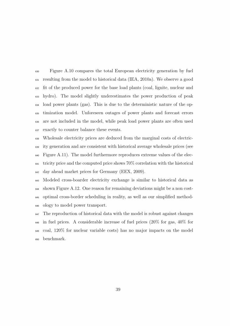
Figure A.10 compares the total European electricity generation by fuel630

resulting from the model to historical data (IEA, 2010a). We observe a good631

fit of the produced power for the base load plants (coal, lignite, nuclear and632

hydro). The model slightly underestimates the power production of peak633

load power plants (gas). This is due to the deterministic nature of the op-634

timization model. Unforeseen outages of power plants and forecast errors635

are not included in the model, while peak load power plants are often used636

exactly to counter balance these events.637

Wholesale electricity prices are deduced from the marginal costs of electric-638

ity generation and are consistent with historical average wholesale prices (see639

Figure A.11). The model furthermore reproduces extreme values of the elec-640

tricity price and the computed price shows 70% correlation with the historical641

day ahead market prices for Germany (EEX, 2009).642

Modeled cross-boarder electricity exchange is similar to historical data as643

shown Figure A.12. One reason for remaining deviations might be a non cost-644

optimal cross-border scheduling in reality, as well as our simplified method-645

ology to model power transport.646

The reproduction of historical data with the model is robust against changes647

in fuel prices. A considerable increase of fuel prices (20% for gas, 40% for648

coal, 120% for nuclear variable costs) has no major impacts on the model649

benchmark.650

39

Transported Energy

TWh

−30

−20

−10

0

10

20

30

40

Transported Energy

TWh

−30

−20

−10

0

10

20

30

40

A_C

ZA

_D A_I

A_S

LO B_F

B_L

uxB

_NL

Ch_

DC

h_F

Ch_

IC

Z_D

CZ_

PL

D_D

KD

_DK

D_F

D_L

uxD

_NL

DK

_DD

K_N

DK

_SE

S_F

ES

_P F_I

H_K

roH

_SK

PL_

SK

Ro_

SR

B

Real TransportModel Results

Figure A.12: Cross-boarder electricity exchange: model results (Base 2008 ) and historicaldata (ENTSO-E, 2010)

Aboumahboub, T., 2011. Development and Application of a Global Electric-651

ity System Optimization Model with a Particular Focus on Fluctuating652

Renewable Energy Sources. Ph.D. thesis, Lehrstuhl fur Energiewirtschaft653

und Anwendungstechnik, Technical University Munich, Prof. U. Wagner.654

Beurskens, F., Hekkenberg, M., 2011. Renewable Energy Projections655

as Published in the National Renewable Energy Action Plans of the656

European Member States Covering all 27 EU Member States. European657

Environment Agency.658

40

URL http://www.ecn.nl/units/ps/themes/renewable-energy/659

projects/nreap/660

Biberacher, M., 2004. Modeling and optimization of future energy system661

using spacial and temporal methods. Ph.D. thesis, Institute of Physics,662

University of Augsburg.663

BMU, 2011. Bundesministerium fur Umwelt, Naturschutz und Reaktor-664

sicherheit: Erneuerbare Energien in Zahlen. BMU, Berlin.665

URL http://www.bmu.de/files/pdfs/allgemein/application/pdf/666

ee_in_zahlen_2010_bf.pdf667

Bofinger, S., von Bremen, L., Knorr, K., Lesch, K., Rohrig, K., Saint-668

Drenan, Y.-M., Speckmann, M., 2008. Raum-zeitliche Erzeugungsmuster669

von Wind- und Solarenergie in der UCTE-Region und deren Einfluss670

auf elektrische Transportnetze: Abschlussbericht fur Siemens Zentraler671

Forschungsbereich (Temporal and spatial generation patterns of wind and672

solar energy in the UCTE region. Impacts of these on the electricity trans-673

mission grid). Institut fur Solare Energieversorgungstechnik, ISET e.V.,674

Kassel.675

Borchert, J., Schemm, R., Korth, S., 2006. Stromhandel: Institutio-676

nen, Marktmodelle, Pricing und Risikomanagement. Schaffer-Poeschel,677

Stuttgart.678

URL http://deposit.ddb.de/cgi-bin/dokserv?id=2803439&679

prov=M&dok_var=1&dok_ext=htm/http://www.gbv.de/dms/bsz/toc/680

bsz25421794xinh.pdf681

41

Bower, J., 2003. A review of european electricity statistics.682

URL http://www.oxfordenergy.org/pdfs/jelsample.pdf683

Czisch, G., 2005. Szenarien zur zukunftigen Stromversorgung , Kostenop-684

timierte Variationen zur Versorgung Europas und seiner Nachbarn mit685

Strom aus erneuerbaren Energien (Scenarios for a future power supply, cost686

optimal scenarios for renewable power supply in Europe and its neighbors).687

Ph.D. thesis, Elektrotechnik / Informatik der Universitat Kassel.688

de Miera, G. S., del Rio Gonzalez, P., Vizcaıno, I., 2008. Analysing the689

impact of renewable electricity support schemes on power prices: The case690

of wind electricity in spain. Energy Policy 36 (9), 3345 – 3359.691

Dena, 2005. Deutsche Energie-Agentur GmbH: Energiewirtschaftliche692

Planung fur die Netzintegration von Windenergie in Deutschland an Land693

und Offshore bis zum Jahr 2020, Endbericht (Energy economic planning694

of grid integration for wind on- and offshore energy in Germany until695

2020).696

URL http://www.dena.de/de/themen/thema-esd/publikationen/697

publikation/netzstudie/698

Dena, 2008. Deutsche Energie-Agentur GmbH: Kurzanalyse der Kraftwerks-699

und Netzplanung in Deutschland bis 2020 (mit Ausblick auf 2030).700

URL http://www.dena.de/themen/thema-esd/projekte/projekt/701

kraftwerks-und-netzplanung/702

Dena, 2010. Deutsche Energie-Agentur GmbH: dena-Netzstudie II: Inte-703

gration enerneuerbarer Energien in die deutsche Stromversorgung im704

42

Zeitraum 2015-2020 mit Ausblick 2025.705

URL http://www.dena.de/themen/thema-esd/projekte/projekt/706

dena-netzstudie-ii707

DLR, 2006. Trans-Mediterranean Interconnection for Concentrating Solar708

Power (TRANS-CSP), Final Report, Study by German Aerospace Center709

(DLR), Institute of Technical Thermodynamics, Section Systems Analysis710

and Technology Assessment and the Federal Ministry for the Environment,711

Nature Conservation and Nuclear Safety, Germany.712

URL http://www.dlr.de/tt/desktopdefault.aspx/tabid-2885/713

4422_read-6588/714

Edenhofer, O., Knopf, B., Barker, T., Baumstark, L., Bellevrat, E., Chateau,715

B., Criqui, P., Isaac, M., Kitous, A., Kypreos, S., Leimbach, M., Lessmann,716

K., Magne, B., Scrieciu, S., Turton, H., Vuuren, D. v., 2010. The Eco-717

nomics of Low Stabilization: Model Comparison of Mitigation Strategies718

and Costs. Energy Journal 31.719

EEX, 2009. European Energy Exchange: German Day-Ahead Electricity720

Market.721

URL www.eex.com722

ENTSO-E, 2009. System Adequacy Retrospect. European Network of Trans-723

mission System Operators.724

ENTSO-E, 2010. European Network of Transmission System Operators for725

Electricity: Statistical Data.726

URL https://www.entsoe.eu/727

43

EPIA, 2009. European Photovoltaic Industry Association & A.T. Kearney:728

Set for Sun.729

URL http://www.setfor2020.eu/730

EPIA (Ed.), 2011. European Photovoltaic Industry Association: Global Mar-731

ket Outlook for Photovoltaics until 2015. EPIA.732

EU Commission, 2006. Commission of the European Communities: Renew-733

able Energy Road Map: Renewable Energies in the 21st century: building734

a more sustainable future. Communication from the Commission to the735

Council and the European Parliament 848.736

EWEA, 2008. European Wind Energy Association: Pure Power - Wind737

Energy Scenarios up to 2030.738

URL http://www.ewea.org/fileadmin/ewea_documents/documents/739

publications/reports/purepower.pdf740

EWEA, 2009a. European Wind Energy Association: A breath of fresh air,741

Annual Report.742

URL http://www.ewea.org/fileadmin/ewea_documents/documents/743

publications/reports/Ewea_Annual_Report_2009.pdf744

EWEA, 2009b. European Wind Energy Association: Oceans of Opportunity:745

Harnessing Europe’s largest domestic energy resource.746

URL http://www.ewea.org/fileadmin/ewea_documents/documents/747

publications/reports/Offshore_Report_2009.pdf748

EXAA, 2010. Energy exchange austria.749

URL www.exaa.at750

44

Giebel, G., 2000. On the Benefits of Distributed Generation of Wind Energy751

in Europe. Ph.D. thesis, Fachbereich Physik der Universitat Oldenburg.752

Green, R., Vasilakos, N., 2010. Market behaviour with large amounts of753

intermittent generation. Energy Policy 38 (7), 3211 – 3220.754

Greenpeace, 3E, 2008. A North Sea electricity grid [r] evolution: electricity755

output of interconnected offshore wind power: a vision of offshore wind756

power integration.757

URL http://www.greenpeace.org/raw/content/eu-unit/758

press-centre/reports/A-North-Sea-electricity-grid-(r)evolution.759

pdf760

GWEC (Ed.), 2011. Global Wind Energy Council: Global Wind Report;761

Annual Market Update 2010. GWEC.762

Haase, T., 2006. Anforderungen an eine durch Erneuerbare Energien gepragte763

Energieversorgung - Untersuchung des Regelverhaltens von Kraftwerken764

und Verbundnetzen (Requirement for power supply with major shares of765

renewables – analysis of the power plant and network control). Ph.D. thesis,766

Fakultat fur Informatik und Eletroktechnik der Universitat Rostock.767

Heide, D., von Bremen, L., Greiner, M., Hoffmann, C., Speckmann, M.,768

Bofinger, S., 2010. Seasonal optimal mix of wind and solar power in a769

future, highly renewable europe. Renewable Energy 35 (11), 2483 – 2489.770

Heitmann, N., 2005. Solution of energy problems with the help of linear pro-771

gramming. Ph.D. thesis, Naturwissenschaftliche Fakultat der Universitat772

Augsburg.773

45

Heitmann, N., Hamacher, T., 2009. Stochastic Model of the German Elec-774

tricity System. Energy Systems: Optimization in the Energy Industry 3,775

365–385.776

IEA, 2010a. International Energy Agency: Electricity Information 2010.777

OECD.778

IEA, 2010b. International energy agency: Interactive renewable energy cal-779

culator: Recabs.780

URL http://www.recabs.org/781

IEA (Ed.), 2010c. International Energy Agency: World Energy Outlook 2010.782

Organisation for Economic Co-operation and Development OECD, Paris.783

IEA (Ed.), 2011. International Energy Agency: World Energy Outlook 2011.784

Organisation for Economic Co-operation and Development OECD, Paris.785

Jacobsen, H. K., Zvingilaite, E., 2010. Reducing the market impact of large786

shares of intermittent energy in Denmark. Energy Policy 38 (7), 3403 –787

3413, large-scale wind power in electricity markets with Regular Papers.788

URL http://www.sciencedirect.com/science/article/pii/789

S0301421510000959790

Kerner, W., 2007. Ten-energy policy; trans-european energy networks: Dg791

tren/c2.792

URL http://www.trade-wind.eu/fileadmin/documents/Seminar_793

UCTE/presentations/7_Kerner_EC.pdf794

Leuthold, F., Jeske, T., Weigt, H., von Hirschhausen, C., 2009. When the795

Wind Blows Over Europe. A Simulation Analysis and the Impact of Grid796

46

Extensions. Electricity Markets Working Papers WP-EM-31.797

URL http://www.tu-dresden.de/wwbwleeg/publications/wp_em_31_798

Leuthold_etal_EU_wind.pdf799

MacCormack, J., Hollis, A., Zareipour, H., Rosehart, W., 2010. The large-800

scale integration of wind generation: Impacts on price, reliability and801

dispatchable conventional suppliers. Energy Policy 38 (7), 3837 – 3846,802

large-scale wind power in electricity markets with Regular Papers.803

McKinsey, KEMA, The Energy Futures Lab at Imperial College London,804

Oxford Economics, European Climate Foundation, 2010. RoadMap 2050:805

A practical guide to a prosperous, low-carbon Europe: Technical Analysis:806

Volume I.807

URL http://www.roadmap2050.eu/808

Neuhoff, K., 2005. Large-scale deployment of renewables for electricity gen-809

eration.810

URL http://oxrep.oxfordjournals.org/cgi/content/abstract/21/811

1/88812

NordPool, 2010. Nordic power exchange.813

URL www.nasdaqomxcommodities.com814

Ockenfels, A., Grimm, V., Zoettl, G., 2008. Strommarktdesign: Preisbildung815

im Auktionsverfahren fur Stromkundenkontrakte an der EEX; Gutachten816

im Auftrag der European Energy Exchange AG zur Vorlage an die817

Sachsiche Borsenaufsicht.818

47

URL http://www.eex.com/de/document/38614/gutachten_eex_819

ockenfels.pdf820

OffshoreGrid, 2010. Offshore wind project: Inventory list of possible wind821

farm locations with installed capacities for the 2020 and 2030 scenarios.822

URL http://www.offshoregrid.eu/index.php/results823

Oko-Institut, 2008. Globales Emissions-Modell Integrierter Systeme824

(GEMIS) Version 4.5.825

URL www.gemis.de826

OMEL, 2010. Mercado de electricidad.827

URL www.omel.es828

Platts, 2009. Data Base Description and Research Methodology: UDI Wold829

Electric Power Plant Data Base (WEPP).830

URL http://www.platts.com/Products/831

worldelectricpowerplantsdatabase832

PWC, PriceWaterHouseCoopers, Potsdam Institute for Climate Impact Re-833

search, International Institute for Applied System Analysis, European Cli-834

mate Forum, 2010. 100% Renewable Energy: A Roadmap to 2050 for835

Europe and North Africa.836

Sensfuss, F., Ragwitz, M., Genoese, M., 2008. The merit-order effect: A837

detailed analysis of the price effect of renewable electricity generation on838

spot market prices in germany. Energy Policy 36 (8), 3086 – 3094.839

TradeWind, 2009. Integrating Wind - TradeWind: Developing Europe’s840

power market for the large-scale integration of wind power, Study by Sintef841

48

Energieforskning AS, Riso DTU, 3E, Kema Nederland BV, Technical842

Research Centre of Finland, Garrad Hassan and Partner Ltd, Tracabel843

Engineering and Deutsche Energie-Agentur GmbH (dena).844

URL http://www.ewea.org/fileadmin/ewea_documents/documents/845

publications/reports/TradeWind_Report_01.pdf846

Twomey, P., Neuhoff, K., 2010. Wind power and market power in competitive847

markets. Energy Policy 38 (7), 3198–3210.848

Weigt, H., Jeske, T., Leuthold, F., von Hirschhausen, C., 2010. Take the849

long way down: Integration of large-scale North Sea wind using HVDC850

transmission. Energy Policy 38 (7), 3164 – 3173.851

Wheeler, D., Ummel, K., 2008. Calculating CARMA: Global Estimation of852

CO2 Emissions from the Power Sector. Center for Global Development853

Working Paper Number 145, 1–36.854

Woo, C., Horowitz, I., Moore, J., Pacheco, A., 2011. The impact of wind855

generation on the electricity spot-market price level and variance: The856

Texas experience. Energy Policy 39 (7), 3939 – 3944, special Section:857

Renewable energy policy and development.858

URL http://www.sciencedirect.com/science/article/pii/859

S0301421511002813860

49