Transmission Systems and the

Telephone Network

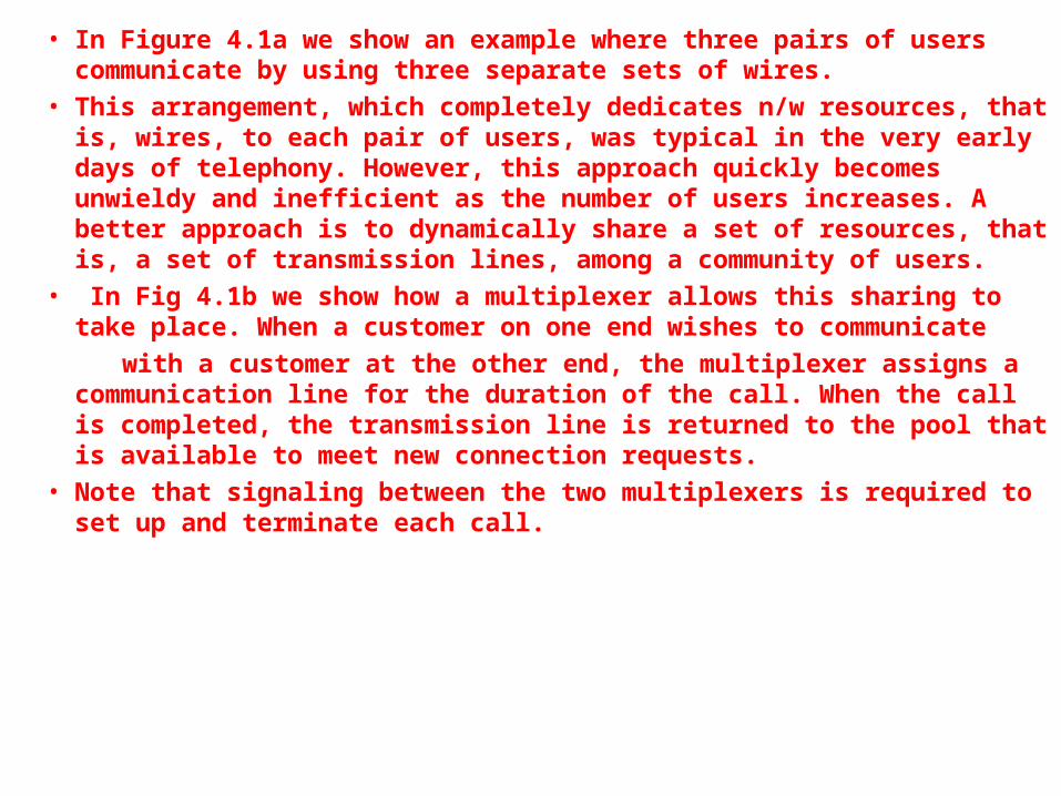
• In Figure 4.1a we show an example where three pairs of users communicate by using three separate sets of wires.

• This arrangement, which completely dedicates n/w resources, that is, wires, to each pair of users, was typical in the very early days of telephony. However, this approach quickly becomes unwieldy and inefficient as the number of users increases. A better approach is to dynamically share a set of resources, that is, a set of transmission lines, among a community of users.

• In Fig 4.1b we show how a multiplexer allows this sharing to take place. When a customer on one end wishes to communicate

with a customer at the other end, the multiplexer assigns a communication line for the duration of the call. When the call is completed, the transmission line is returned to the pool that is available to meet new connection requests.

• Note that signaling between the two multiplexers is required to set up and terminate each call.

• The transmission lines connecting the two multiplexers are called trunks.

• Initially each trunk consisted of a single transmission line; that is, the information signal for one connection was carried in a single transmission line. However,

advances in transmission technology made it possible for a single transmission line of large bandwidth to carry multiple connections. From the point of view of

setting up connections, such a line can be viewed as being equivalent to a number of trunks. In the remainder of this section, we discuss several approaches to

combining the information from multiple connections into a single line.

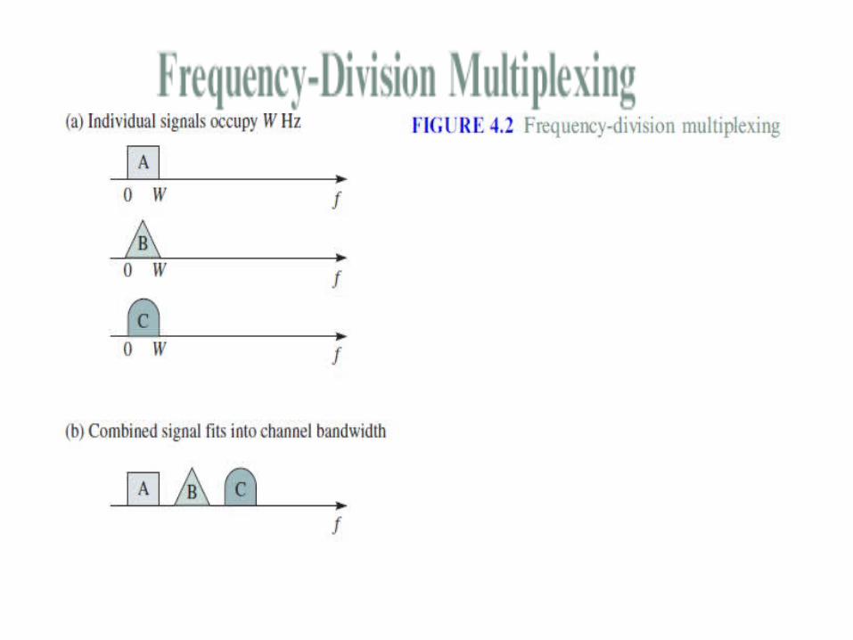
Fig.4.2FFFFF

• Suppose that the transmission line has a bandwidth (measured in Hertz) that is much greater than that required by a single connection. For example, in Figure 4.2a each user has a signal of W Hz, and the channel that is available is greater than 3W Hz.

• In frequency-division multiplexing (FDM), the bandwidth is divided into a number of frequency slots, each of which can accommodate the signal of an individual connection.

• The multiplexer assigns a frequency slot to each connection and uses modulation to place the signal of the connection in the appropriate slot.

• This process results in an overall combined signal that carries all the connections as shown in Figure 4.2b. The combined signal is transmitted, and the demultiplexer recovers the signals corresponding to each connection.

• Reducing the number of wires that need to be handled reduces the overall cost of the system.

• FDM was introduced in the telephone network in the 1930s. The basic analog multiplexer combines 12 voice channels in one line. Each voice signal occupies 4 kHz of bandwidth. The multiplexer modulates each voice signal so that it occupies a 4 kHz slot in the band between 60 and 108 kHz.

• The combined signal is called a group. A hierarchy of analog multiplexers has been defined. For example, a super group (that carries 60 voice signals) is formed by multiplexing

five groups, each of bandwidth 48 kHz, into the frequency band from 312 to 552 kHz.

• Note that for the purposes of multiplexing, each group is treated as an individual signal. Ten super groups can then be multiplexed to form a master group of 600 voice signals that occupies the band 564 to 3084 kHz.

• Various combinations of mastergroups have also been defined.

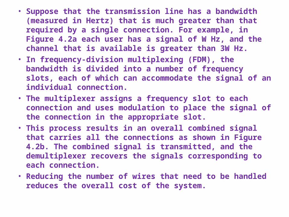
• In time-division multiplexing (TDM), the transmission between the multiplexers is provided by a single high-speed digital transmission line. Each connection produces a digital information flow that is then inserted into the high-speed line.

• For example in Figure 4.3a each connection generates a signal that produces one unit of information every 3T seconds. This unit of information could be a bit, a byte, or a fixed-size block of bits. Typically, the transmission line is organized into frames that in turn are divided into equal-sized slots.

• For example, in Figure 4.3b the transmission line can send one unit of information every T seconds, and the combined signal has a frame structure that consists of three slots, one for each user. During connection setup each connection is assigned a slot that can accommodate the information produced by the connection.

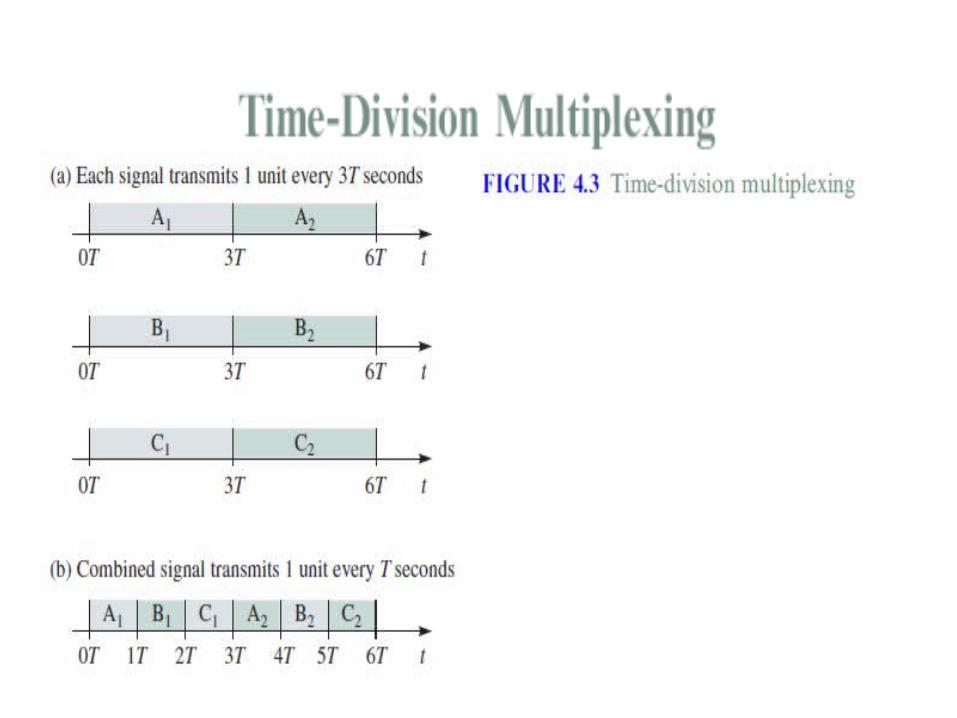
• The T-1 carrier system that carries 24 digital telephone connections is shown in Figure 4.4. Recall that a digital telephone speech signal is obtained by sampling a speech waveform 8000 times/second and by representing each sample with eight bits.

• The T-1 system uses a transmission frame that consists of 24 slots of eight bits each. Each slot carries one PCM sample for a single connection.

• The beginning of each frame is indicated by a single bit that follows a certain periodic pattern.

• The resulting transmission line has a speed of (1 + 24 x 8) bits/frame x 8000 frames/second = 1.544 Mbps

• Note how in TDM the slot size and the repetition

rate determines the bit rate of the individual connections.

• The T-1 carrier system was introduced in 1961 to carry the traffic between telephone central offices.

• The growth of telephone network traffic and the advances in digital transmission led to the development of a standard digital multiplexing hierarchy.

• These digital transmission hierarchies define the global flow of telephone traffic.

• Figure 4.5 shows the digital transmission hierarchies that were developed in North America and Europe. In North America and Japan, the digital signal 1 (DS1), which corresponds to the output of a T-1 multiplexer, became the basic building block.

• The DS2 signal is obtained by combining 4 DS1 signals.

• And the DS3 is obtained by combining 28 DS1 signals. The DS3 signal, with a speed of 44.736 Mbps, has found extensive use in providing high-speed communications to large users such as corporations.

• In Europe the CCITT developed a similar digital hierarchy. The CEPT-1 (also referred to as E1) signal consisting of thirty two 64-kilobit channels forms the basic building block.

• Only 30 of the 32 channels are used for voice channels; one of the other channels is used for signaling, and the other channel is used for frame alignment and link maintenance.

• The second, third, and fourth levels of the hierarchy are obtained by grouping four of the signals in the lower level, as shown in Figure 4.5.

• The operation of a time-division multiplexer involves tricky problems with the synchronization of the input streams. Fig4.6 shows two streams, each with a nominal rate of one bit every T seconds, that are combined into a stream that sends two bits every T seconds.

• What happens if one of the streams is slightly slower than 1/T bps? Every T seconds, the multiplexer expects each input to provide a one-bit input; at some point the slow input will fail to produce its input bit. We will call this event a bit slip. Note that the ``late'' bit will be viewed as an ``early'' arrival in the next T -second interval.

• Thus the slow stream will alternate between being late, undergoing a bit slip, and then being early. Now consider what happens if one of the streams is slightly fast. Because bits are arriving faster than they can be sent out, bits will accumulate at the multiplexer and eventually be dropped.

• To deal with the preceding synchronization problems, time-division multiplexers have traditionally been designed to operate at a speed slightly higher than the combined speed of the inputs.

• The frame structure of the multiplexer output signal contains bits that are used to indicate to the receiving multiplexer that a slip has occurred. This approach enables the streams to be demultiplexed correctly.

• Note that the introduction of these extra bits to deal with slips implies that the frame structure of the output stream is not exactly synchronized to the frame structure of all the input streams. To extract an individual input stream from the combined signal, it is necessary to demultiplex the entire combined signal, make the adjustments for slips, and then remove the desired signal. This type of multiplexer is called ``asynchronous'' because the input frames are not synchronized to the output frame

SONET

1. SONET Multiplexing2. SONET Frame Structure

What is SONET?• In 1966 Charles Kao reported the feasibility of

optical fibers that could be used for communications. By 1977 a DS3 45 Mbps fiber optic system was demonstrated in Chicago, Illinois. By 1998, 40 Gbps fiber optic transmission systems had become available.

• The advances in optical transmission technology have occurred at a rapid rate, and the backbone of telephone networks has become dominated by fiber optic digital transmission systems

• The 1st generation of equipment for optical fiber transmission was proprietary, and no standards were available for the interconnection of equipment from different vendors.

• The deregulation of telecommunications in the United States led to a situation in which the long-distance carriers were expected to provide the

interconnection between local telephone service providers.

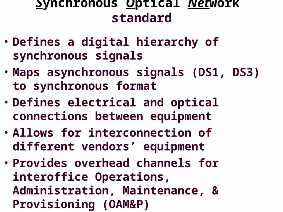
• To meet the urgent need for standards to interconnect optical transmission systems, the Synchronous Optical Network (SONET) standard was developed in North America.

• The CCITT later developed a corresponding set of standards called Synchronous Digital Hierarchy (SDH). SONET and SDH form the basis for current high- speed backbone networks.

Synchronous Optical Network standard

• Defines a digital hierarchy of synchronous signals

• Maps asynchronous signals (DS1, DS3) to synchronous format

• Defines electrical and optical connections between equipment

• Allows for interconnection of different vendors’ equipment

• Provides overhead channels for interoffice Operations, Administration, Maintenance, & Provisioning (OAM&P)

SONET Multiplexing• The SONET standard uses a 51.85 Mbps signal as a

building block to extend the digital transmission hierarchy into the multi gigabit range.

• SONET incorporates extensive capabilities for the operations, administration, and maintenance (OAM) functions that are required to operate digital transmission facilities.

• Table 4.1 shows the SONET and SDH digital hierarchy. The synchronous transport signal level-1 (STS-1) is the basic building block of the SONET hierarchy.

• A higher-level signal in the hierarchy is obtained through the interleaving of bytes from the lower-level component signals. Each STS-n electrical signal has a corresponding optical carrier level-n (OC-n) signal

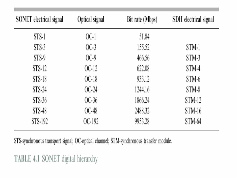
• The bit format of STS-n and OC-n signals is the same except for the use of scrambling in the optical signal.

• The SDH standard refers to synchronous transfer modules-n (STM-n) signals and begins at a bit rate of 155.52 Mbps.

• The SDH STM-1 signal is equivalent to the SONET STS-3 signal. The STS-1 signal accommodates the

DS3 signal from the existing digital transmission hierarchy in North America.

• The STM-1 signal accommodates the CEPT-4 signal in the CCITT digital hierarchy. The STS-48 signal is widely deployed in the backbone of modern

communication networks.• SONET uses a frame structure that has the same 8 kHz repetition rate as traditional TDM systems.

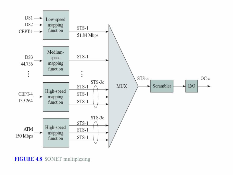
• SONET was designed to be very flexible in the types of traffic that it can handle. SONET uses the term tributary to refer to the component streams that are multiplexed together.

• Fig 4.8 shows how a SONET multiplexer can handle a wide range of tributary types. A slow-speed mapping function allows DS1, DS2, and CEPT-1 signals to be combined into an STS-1

signal. As indicated above DS3 signal can be mapped into an STS-1 signal, and a CEPT-4 signal can be mapped into an STS-3 signal.

• A mapping has also been defined for mapping ATM streams into an STS-3 signal.

• A SONET multiplexer can then combine STS input signals into a higher-order STS-n signal.

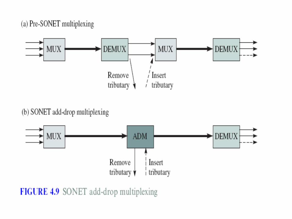
• Asynchronous multiplexing systems prior to SONET required the entire multiplexed stream to be demultiplexed to access a tributary, as shown in Fig 4.9a.

• Transit tributaries would then have to be remultiplexed onto the next hop. Thus every point of tributary removal or insertion required a demul-

tiplexer-multiplexer pair. • SONET produced significant reduction in cost by enabling add-drop multiplexers (ADM) to insert

and extract tributary streams without disturbing tributary streams that are in transit as shown in Figure 4.9b.

• SONET accomplishes this process through the use of pointers that identify the location of a tributary within a frame.

• ADMs in combination with SONET equipment allow distant switching nodes to be connected by tributaries. This arrangement allows the network operator to define networks of switching nodes with arbitrary topologies.

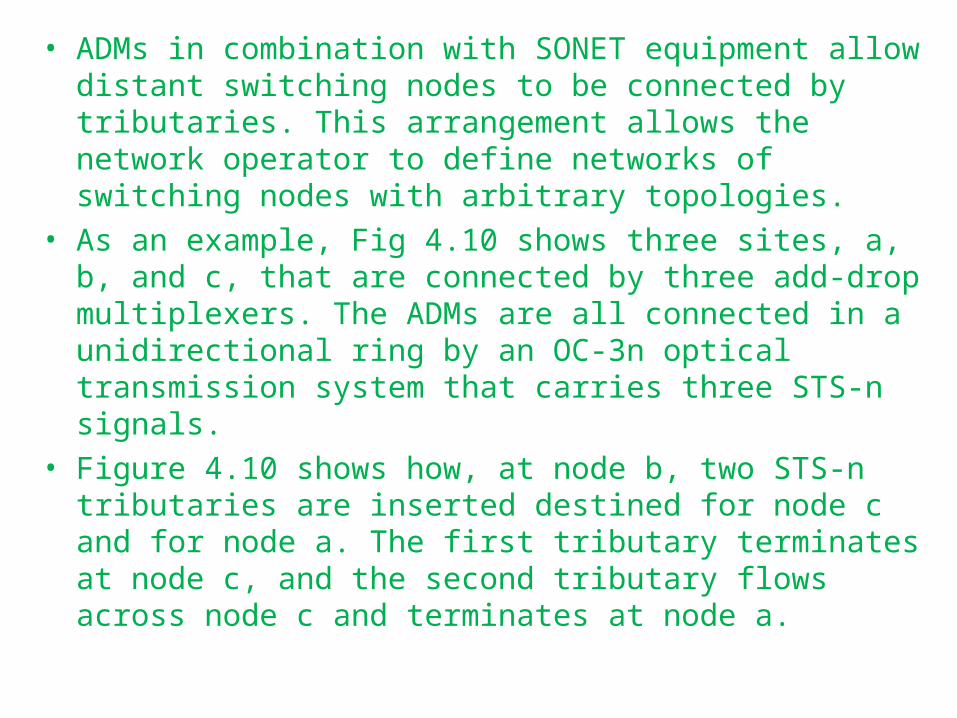
• As an example, Fig 4.10 shows three sites, a, b, and c, that are connected by three add-drop multiplexers. The ADMs are all connected in a unidirectional ring by an OC-3n optical transmission system that carries three STS-n signals.

• Figure 4.10 shows how, at node b, two STS-n tributaries are inserted destined for node c and for node a. The first tributary terminates at node c, and the second tributary flows across node c and terminates at node a.

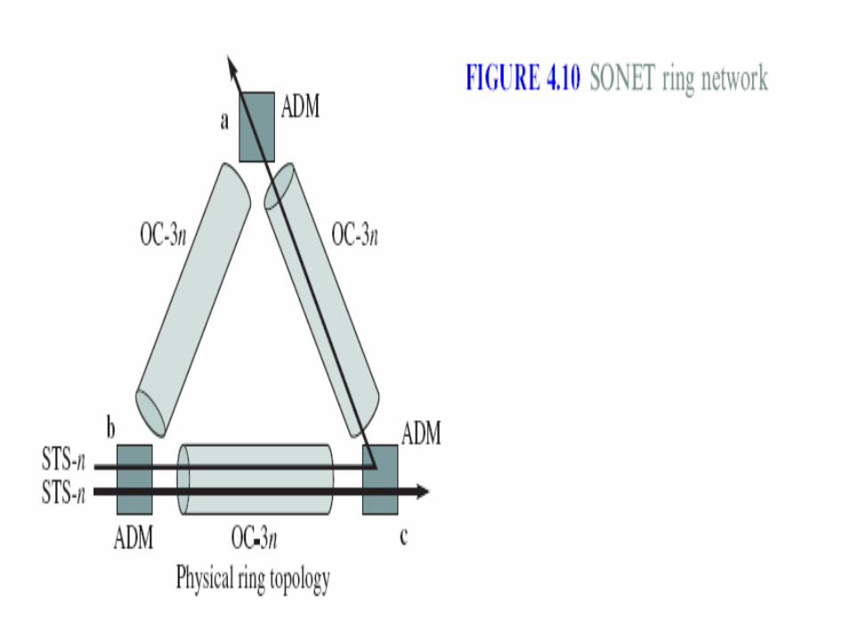
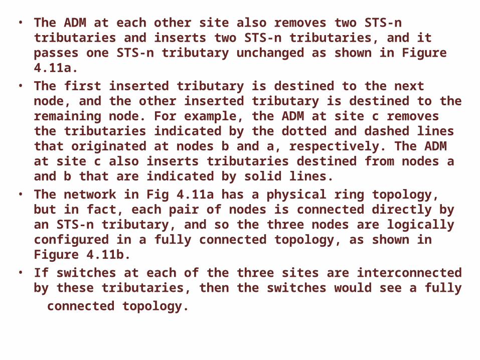
• The ADM at each other site also removes two STS-n tributaries and inserts two STS-n tributaries, and it passes one STS-n tributary unchanged as shown in Figure 4.11a.

• The first inserted tributary is destined to the next node, and the other inserted tributary is destined to the remaining node. For example, the ADM at site c removes the tributaries indicated by the dotted and dashed lines that originated at nodes b and a, respectively. The ADM at site c also inserts tributaries destined from nodes a and b that are indicated by solid lines.

• The network in Fig 4.11a has a physical ring topology, but in fact, each pair of nodes is connected directly by an STS-n tributary, and so the three nodes are logically configured in a fully connected topology, as shown in Figure 4.11b.

• If switches at each of the three sites are interconnected by these tributaries, then the switches would see a fully

connected topology.

• This approach allows the configuration of arbitrary logical topologies with arbitrary link transmission rates. Further more, this configuration can be done using software control. Thus we see that the introduction of SONET equipment provides the network operator with tremendous flexibility in managing the transmission resources to meet the user requirements.

• SONET systems can be deployed in the form of self-healing rings. Such rings provide two paths between any two nodes in the ring, thus providing for fault recovery in the case of single node or link failure. Figure 4.12a shows a two fiber ring in which data is copied in both fibers, one traveling clockwise and the other counterclockwise. In a normal operation one fiber (clockwise) is in a working mode, while another (counterclockwise) is in a protect mode.

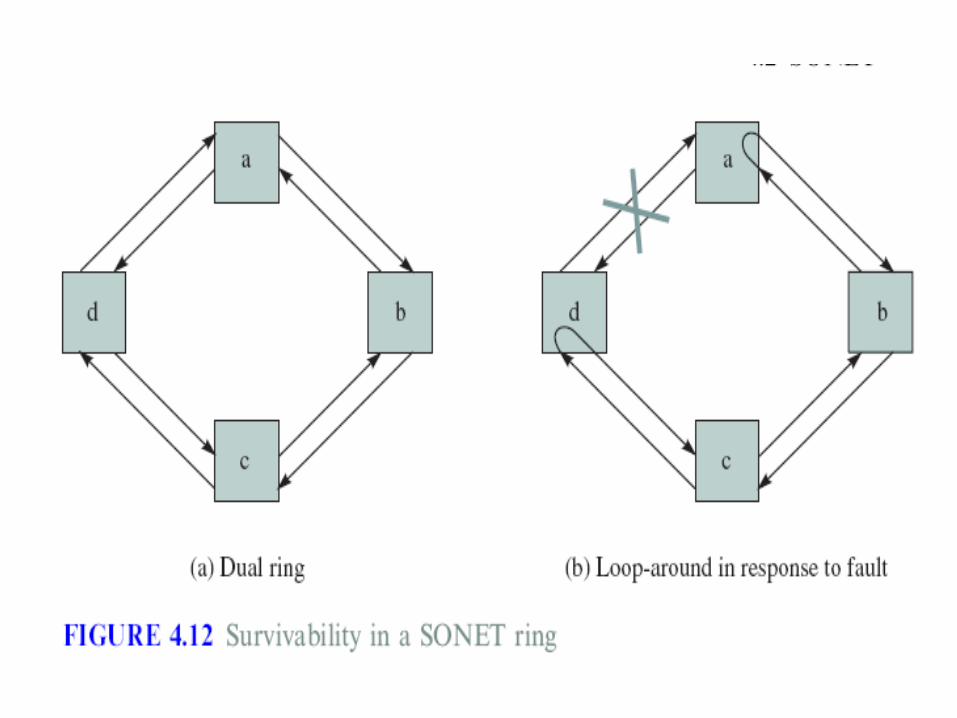
• When the fibers between two nodes are broken, the ring wraps around as shown in Figure 4.12b.

• Traffic continues to flow for all tributaries. A similar procedure is carried out in case of a node failure. In this case traffic is redirected by the two nodes adjacent to the affected node. Only traffic to the faulty node is discontinued.

• SONET ring networks typically recover from these types of faults in less than 50 millisec,depending on the length of the ring, which can span diameters of several thousand kilometers. The preceding discussion assumes a ``unidirectional' ring.

• A SONET ring can also be bidirectional, in which case working traffic travels in both directions. Furthermore, a SONET ring can have either two fibers or four fibers per link.

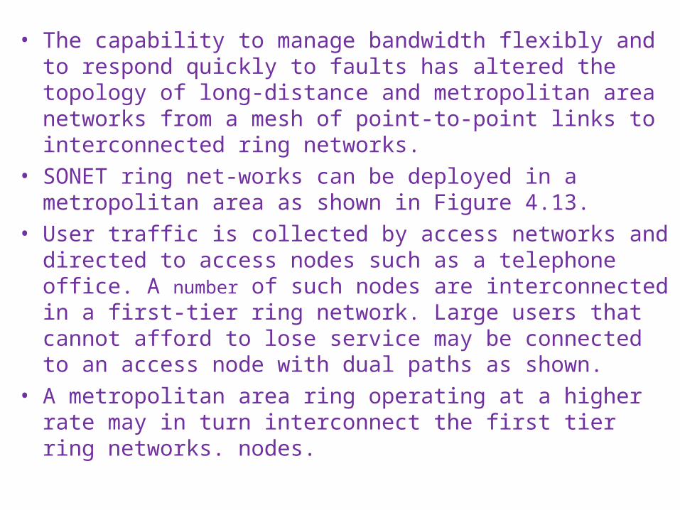
• The capability to manage bandwidth flexibly and to respond quickly to faults has altered the topology of long-distance and metropolitan area networks from a mesh of point-to-point links to interconnected ring networks.

• SONET ring net-works can be deployed in a metropolitan area as shown in Figure 4.13.

• User traffic is collected by access networks and directed to access nodes such as a telephone office. A number of such nodes are interconnected in a first-tier ring network. Large users that cannot afford to lose service may be connected to an access node with dual paths as shown.

• A metropolitan area ring operating at a higher rate may in turn interconnect the first tier ring networks. nodes.

• To provide protection against faults, rings may be interconnected by using matched inter-ring gateways as shown between the interoffice ring and the metro ring and between the metro ring and the regional ring.

• The traffic flow between the rings is sent simultaneously along the primary and secondary gateway. Automated protection procedures determine whether the primary or secondary incoming

traffic is directed into the ring. • The metropolitan area ring, in turn, may connect to the ring of an interexchange or regional carrier as

shown in the figure.• Several variations of SONET rings can be deployed to

provide survivability. The merits of the approaches depend to some extent on the size of the ring and the pattern of traffic flows between nodes.

SONET Frame Structure• A SONET system is divided into three layers: sections,

lines, and paths as shown in Fig4.14a.• A section refers to the span of fiber between two

adjacent devices, such as two repeaters. The section layer deals with the transmission of an STS-n signal across the physical medium.

• A line refers to the span between two adjacent multiplexers and therefore in general encompasses

several sections. Lines deal with the transport of an aggregate multiplexed stream of user information and the associated overhead.

• A path refers to the span between the two SONET terminals at the endpoints of the system and in

general encompasses one or more lines.

• In general the multiplexers associated with the path level, for example, STS-1, are lower in the hierarchy than the muxers in the line level, for example,S TS-3 or STS-48, as Fig 4.14a. The reason is that a typical information flow begins at some bit rate at the edge of the network, which is then combined into higher-level aggregate flows inside the network, and finally delivered back at the original lower bit rate at the outside edge of the network.

• Fig 4.14b shows that every section has an associated optical layer. The section layer deals with the signals in their electrical form, and the optical layer deals with the transmission of optical pulses. It can be seen that every regenerator involves converting the optical signal to electrical form to carry out the regeneration function and then back to optical form. Note also in Fig4.14b that all of the equipment implements the optical and section functions.

• Line functions are found in the multiplexers and end terminal equipment.

• The path function occurs only at the end terminal equipment.

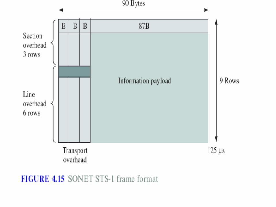
• Figure 4.15 shows the structure of the SONET STS-1 frame that is defined at the line level. A frame consisting of a rectangular array of bytes arranged in 9 rows by 90 bytes is repeated 8000 times a second. And the overall bit rate of the STS-1 is

8 x 9 x 90 x 8000 = 51.84 Mbps• The first three columns of the array are allocated to section and

line overhead. The section overhead is interpreted and modified at every section termination and is used to provide framing, error monitoring, and other section-related

management functions. • The line overhead is interpreted and modified at every line termination and is used to provide synchronization and

multiplexing for the path layer, as well as protection-switching capability.

• We will see that the first three bytes of the line overhead play a crucial role in how multiplexing is carried out. The remaining 87 columns of the frame constitute the information payload that carries the path layer information.

• The bit rate of the information payload is 8 x 9 x 87 x 8000 = 50.122 Mbps• The information payload includes one column of path overhead

information, but the column is not necessarily aligned to the frame for reasons that will soon become apparent.

• Consider next how the end-to-end user information is organized at the path level. The user data and the path overhead are included in the synchronous pay-load envelope (SPE), which consists of a byte array of 87 columns by nine rows, as shown in Fig4.16. The path overhead constitutes the first column of this array. This SPE is then inserted into the STS-1 frame. The SPE is not necessarily aligned to the information payload of an STS-1 frame. Instead, the first two bytes of the line overhead are used as a pointer that indicates the byte within the information payload where the SPE begins.

• Consequently, the SPE can be spread over two consecutive frames as shown in Fig 4.16. The use of the pointer makes it possible to extract a tributary signal from the multiplexed signal. This feature gives SONET its add-drop capability.

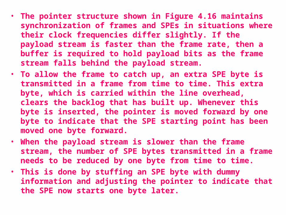
• The pointer structure shown in Figure 4.16 maintains synchronization of frames and SPEs in situations where their clock frequencies differ slightly. If the payload stream is faster than the frame rate, then a buffer is required to hold payload bits as the frame stream falls behind the payload stream.

• To allow the frame to catch up, an extra SPE byte is transmitted in a frame from time to time. This extra byte, which is carried within the line overhead, clears the backlog that has built up. Whenever this byte is inserted, the pointer is moved forward by one byte to indicate that the SPE starting point has been moved one byte forward.

• When the payload stream is slower than the frame stream, the number of SPE bytes transmitted in a frame needs to be reduced by one byte from time to time.

• This is done by stuffing an SPE byte with dummy information and adjusting the pointer to indicate that the SPE now starts one byte later.

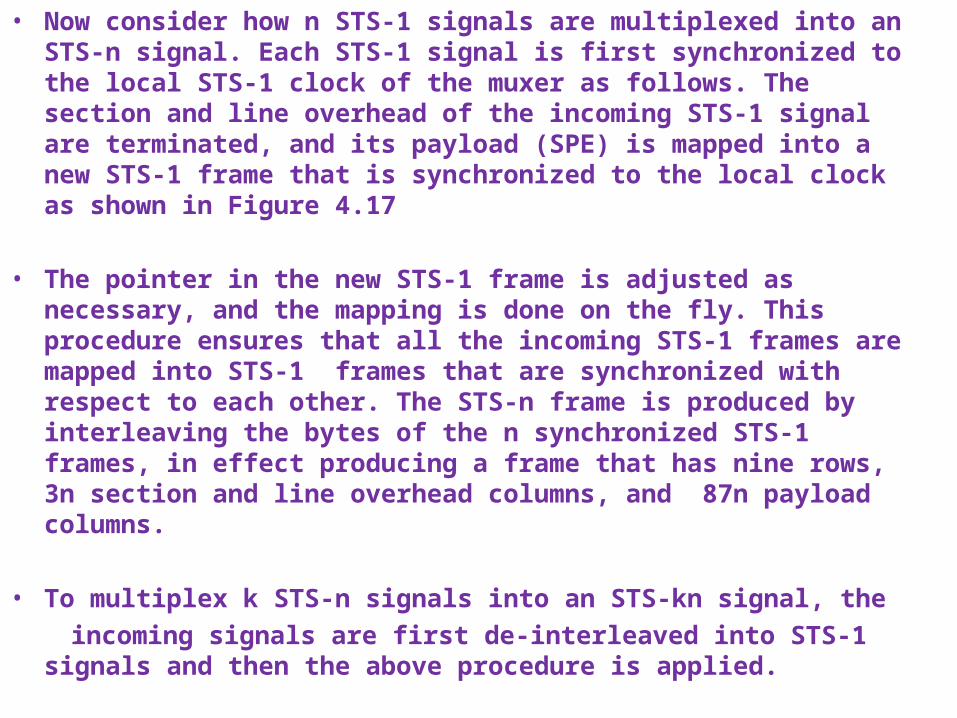
• Now consider how n STS-1 signals are multiplexed into an STS-n signal. Each STS-1 signal is first synchronized to the local STS-1 clock of the muxer as follows. The section and line overhead of the incoming STS-1 signal are terminated, and its payload (SPE) is mapped into a new STS-1 frame that is synchronized to the local clock as shown in Figure 4.17

• The pointer in the new STS-1 frame is adjusted as necessary, and the mapping is done on the fly. This procedure ensures that all the incoming STS-1 frames are mapped into STS-1 frames that are synchronized with respect to each other. The STS-n frame is produced by interleaving the bytes of the n synchronized STS-1 frames, in effect producing a frame that has nine rows, 3n section and line overhead columns, and 87n payload columns.

• To multiplex k STS-n signals into an STS-kn signal, the incoming signals are first de-interleaved into STS-1

signals and then the above procedure is applied.

4.3:Wavelength Division Multiplexing

• Current optical fiber transmission systems can operate at bit rates in the tens ofGbps. The underlying available electronics technologies have a maximum speed limit in the tens of Gbps.

• Similarly, laser diodes can support bandwidths in the tens of GHz. In the case of low attenuation wavelengths about 100 nm wide is available in the 1300 nm range.

• This range corresponds to a BW of 18 terahertz (THz). Another band of about 100 nm in the 1550 nm range provides 19 THz of BW

• Recall that 1 THz = 1000 GHz. Clearly the available technology does not come close to exploiting the available bandwidth.

• The information carried by a single optical fiber can be increased through the use of wavelength-division multiplexing (WDM). WDM can be viewed as an optical-domain version of FDM in which multiple information signals modulate optical signals at different optical wavelengths (colors).

• The resulting signals are combined and transmitted simultaneously over the same optical fiber as shown in Figure 4.18.

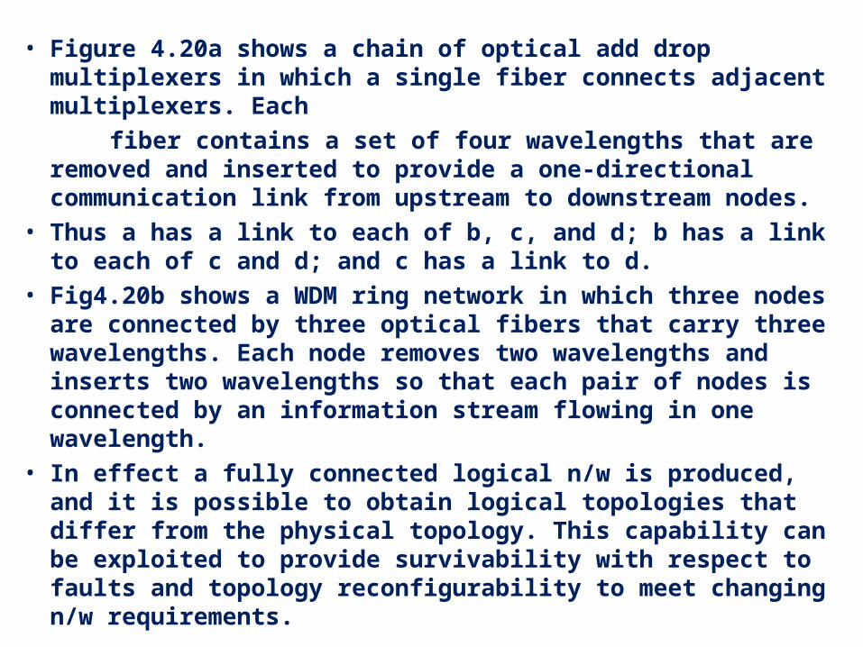
• Figure 4.20a shows a chain of optical add drop multiplexers in which a single fiber connects adjacent multiplexers. Each

fiber contains a set of four wavelengths that are removed and inserted to provide a one-directional communication link from upstream to downstream nodes.

• Thus a has a link to each of b, c, and d; b has a link to each of c and d; and c has a link to d.

• Fig4.20b shows a WDM ring network in which three nodes are connected by three optical fibers that carry three wavelengths. Each node removes two wavelengths and inserts two wavelengths so that each pair of nodes is connected by an information stream flowing in one wavelength.

• In effect a fully connected logical n/w is produced, and it is possible to obtain logical topologies that differ from the physical topology. This capability can be exploited to provide survivability with respect to faults and topology reconfigurability to meet changing n/w requirements.

• The introduction of WDM and optical Add Drop Mux into a n/w adds a layer of logical abstraction b/w the physical topology & the logical topology that is seen by the systems that send traffic flows through the network.

• The physical topology consists of the optical Add Drop Mux interconnected with a number of optical fibers. The manner in which light paths are defined by the optical ADMs in the WDM system determines the topology that is seen by SONET ADMs that are interconnected by these light paths.

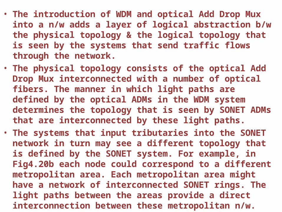
• The systems that input tributaries into the SONET network in turn may see a different topology that is defined by the SONET system. For example, in Fig4.20b each node could correspond to a different metropolitan area. Each metropolitan area might have a network of interconnected SONET rings. The light paths between the areas provide a direct interconnection between these metropolitan n/w.

• In WDM each wavelength is modulated separately, so each wavelength need not carry information in the same transmission format. Thus some wavelengths might carry SONET formatted information streams, while others might carry

• Gigabit Ethernet formatted information or other transmission formats.

4.4:Circuit Switches

• A n/w is frequently represented as a cloud that connects multiple users as shown in Figure 4.21a. A circuit-switched network is a generalization of a physical cable in the sense that it provides connectivity that allows information to flow b/w inputs and outputs to the n/w. Unlike a cable, however, a network is geographically distributed and consists of a graph of transmission lines (that is, links) interconnected by switches (nodes).

• As shown in Fig4.21b, the function of a circuit switch is to transfer the signal that arrives at a given input to an appropriate output. The interconnection of a sequence of transmission links and circuit switches enables the flow of information b/w inputs and outputs in the n/w.

4.4.1 Space-Division Switches

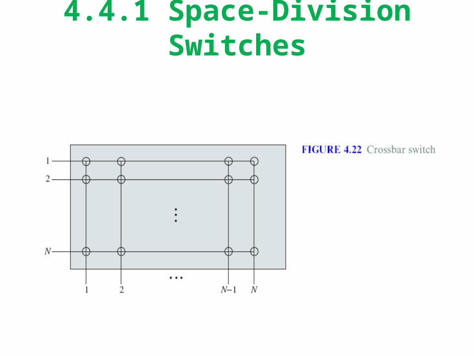
• The first switches we consider are called space-division switches because they provide a separate physical connection between inputs and outputs so the different signals are separated in space. Fig 4.22 shows the crossbar switch, which is an example of this type of switch. The crossbar switch consists of an nxn array of cross points that can connect any input to any available output.

• When a request comes in from an incoming line for an outgoing line, the corresponding cross point is closed to enable information to flow from the input to the output. The crossbar switch is said to be nonblocking; in other words, connection requests are never denied because of lack of connectivity resources, that is, cross points.

• Connection requests are denied only when the requested outgoing line is already engaged in another connection.

• The complexity of the crossbar switch as measured by the number of cross points is N2(square)

• . This number grows quickly with the number of input and output ports. Thus a 1000-input-by-1000-output switch requires 10 power 6

crosspoints, and a 100,000 by 100,000 switch requires 10 power 10 crosspoints. In the next section.

• Number of crosspoints can be reduced by using multistage switches.

• Fig 4.23 shows a multistage switch that consists of three stages of smaller space-division switches. The N inputs are grouped into N/n groups of n input lines. Each group of n input lines enters a small switch in the first stage that consists of an n x n array of cross points.

• Each input switch has one line connecting it to each of k intermediate stage N/n x N/n switches. Each intermediate

switch in turn has one line connecting it to each of the N/n switches in the third stage. The latter switches are k  n. In effect each set of n input lines shares k

• possible paths to any one of the switches at the last stage; that is, the ®rst path goes

• through the ®rst intermediate switch, the second path goes through the second

• intermediate switch, and so on. The resulting multistage switch is not necessarily

• nonblocking. For example, if k < n, then as soon as a switch in the ®rst stage has

• k connections, all other connections will be blocked.