transmission talk ieee...
TRANSCRIPT

Transmission Lines – Electricity’s Highway
This talk starts with an explanation of Surge Impedance Loading and demonstrates how it is used for transmission line work. The St. Clair Curve widely used in transmission work is illustrated along with its development. Reactive power requirements are illustrated and its importance to transmission line engineering is illustrated. Included in talk are examples of calculations that can and should be done before undertaking any detailed power system studies.
Date: March 9th, 2015
Time:
Place:
Speaker’s Biography
W.O. (Bill) Kennedy, (LSMIEEE) is President and Principal of b7kennedy & Associates Inc., a consulting company he established in 2005 to provide service to companies connecting to the electric power grid. Throughout his 45 year career he has worked on the Nelson River HVDC transmission system, 500 kV transmission in Pakistan, 400 kV transmission in Iran and 138 kV transmission in Peru. Bill has worked or consulted in nine of Canada’s ten provinces. He has developed successful and innovative power system seminars to educate non-power system engineers and other engineers on how the electric power system works.
His accomplishments include the development of a distance relay testing procedure that allowed the relays to be tested insitu. This procedure moved relay testing from the shop floor to the substation. Bill demonstrated that import on the 500 kV transmission line connecting Alberta to British Columbia could be raised to 600 MW without the requirement for load shed in Alberta. He developed transmission required to incorporate 3,400 MW of wind based energy into the Alberta grid. Using a Stakeholder consultative approach, he developed the first protection standard for Alberta. While a utility employee, Bill lead the development of a 455 km 138 kV transmission line in northern Saskatchewan effectively incorporating northern communities into the SaskPower grid.
Bill is the author of 15 papers and lectures on transmission lines and other power system topics.
Active in IEEE Bill served two terms as Director for IEEE Canada (Region 7) and for PES (Division VII). He was general chair of 2009 Power and Energy General Meeting held in Calgary. At the time, it was the largest PES General Meeting ever held. He is the General Chair of EPEC 2014 which was held in Calgary in November of 2014.
Bill is a registered engineer in Alberta. He is a member of CIGRE and the IEEE Standards Association. Bill was the Y2K coordinator for Alberta transmission system. He was a member of the NERC Task Force investigating issues from the 2003 Blackout.
His expertise was recognized by the Engineering Institute of Canada when Bill was elected Fellow in 1998. In 2009 he was the University of New Brunswick’s Dineen Lecturer.
In addition, Bill was recognized by IEEE Canada as the 2014 Outstanding Engineer and he is the 2015 recipient of the IEEE Canada Power Medal.

3/11/2015
1
Transmission LinesElectricity's Highways
W.O. (Bill) Kennedy, P.Eng., FEIC
President & Principal
© 2015 b7kennedy & Associates Inc. 1
b7kennedy & Associates Inc.
Introduction
• Transmission lines are the highways for electricity.
• Their main purpose is to connect load to generation.
• Electricity in the context that I’ll use it includes both power and energy.
• Transmission lines are a civil, mechanical and electrical engineering challenge.
• This talk will focus on the electrical aspects of transmission lines.
© 2015 b7kennedy & Associates Inc. 2

3/11/2015
2
© 2015 b7kennedy & Associates Inc. 3
Transmission lines
• For the power system, there are all types of transmission lines from low voltage to high voltage.
• Each has its own purpose and each has a fixed amount of electricity transfer capability.
• Transmission lines are complex devices influenced by system voltages, loading, physical properties, system reactive capability and stability.
• We’ll examine each of these.• We will start with Surge Impedance Loading (SIL).• SIL is an important property of transmission lines.
SURGE IMPEDANCE LOADING
© 2014 b7kennedy & Associates Inc. 4

3/11/2015
3
© 2015 b7kennedy & Associates Inc. 5
Surge Impedance Loading (SIL)
• Transmission line consists of:– Shunt capacitance
– Series resistance and inductance
– Distributed along length of line
• Treat as distributed lumped elements
• Can ignore resistance
© 2015 b7kennedy & Associates Inc. 6
Surge Impedance Loading (SIL)
• Close the breaker at sending end
• Shunt capacitance charges to ½ CV2
• Close the breaker at receiving end and feed the load
• Series inductance consumes energy at ½ LI2

3/11/2015
4
© 2015 b7kennedy & Associates Inc. 7
Surge Impedance Loading (SIL)
Equating shunt and series energies
½ CV2 = ½ LI2
Performing the math yields
SIL (power) = V2/SI
© 2015 b7kennedy & Associates Inc. 8
System Model
• We need to develop a system model.• We will assume two machines at each end of our line.• Each machine will have sufficient reactive power
capability to supply and absorb the reactive power from/to the line.
• We know we can ‘collapse’ any power system to a two machine equivalent.
• Effectively, we’re developing a Thévenin voltage behind a Thévenin impedance.
• For the Thévenin impedance, we’ll use the breaker’s three phase fault rating.

3/11/2015
5
© 2015 b7kennedy & Associates Inc. 9
System Model
• There are three line models.• The first is the open circuit line. That is, how does a
transmission line open circuited at the receiving end behave? We’ll deal with this briefly.
• The second is the line with active and reactive power sources at both ends. This will be the subject to the seminar.
• The third is the line that has an active and reactive power source at the sending and a load at the receiving end.
• That is, the receiving end has no reactive power generation capability. We will not be discussing this type of line.
SIL Example
© 2015 b7kennedy & Associates Inc. 10
slack
0 MW
-106.75 Mvar
Send Bus Rec Bus
MW 0
0.00 Mvar
1.00 pu 0.00 Deg
1.03 pu-0.00 Deg
A
MVA
0.00 MW-106.75 Mvar
0.00 MW 0.00 Mvar

3/11/2015
6
© 2015 b7kennedy & Associates Inc. 11
Properties of Surge Impedance (SI)
• Remains fairly constant over a wide range of voltages.• Starts around 400 Ω at lower voltages and decreases
with bundling to around 225 Ω at 1500 kV.• Bundling – use of more than one conductor per phase.• Capacitance and inductance also remain fairly constant.• Using this, we can construct the following table.• Conductor size is expressed thousand circular mils or
MCM. MCM is an expression of conductor current carrying area.
• Capacitance or charging is expressed as kVAr/km.• R and X are in Ω/km or ohms/km.
© 2015 b7kennedy & Associates Inc. 12
Conductor Bundling
• Bundling is required at higher voltages.• Bundling is the use of two or more conductors per
phase.• Bundling reduces the series inductance and increases
the shunt capacitance.• The effect is to decrease SI and increase SIL.

3/11/2015
7
Properties of Transmission Lines
© 2015 b7kennedy & Associates Inc. 13
Voltage (kV)
Conductor (MCM)
SI (Ω) R (Ω/km) X (Ω/km)Charging (kVAr/km)
SIL (MW)
72 266 390 0.41 0.5 17 15
138 477 386 0.14 0.5 63 50
230 (single)
795 384 0.09 0.5 176 150
230 (bundled)
2x795 281 0.04 0.4 247 190
345 (bundled)
3x795 257 0.03 0.3 605 460
500 (bundled)
4x795 238 0.02 0.3 1,339 1050
ST. CLAIR CURVE
© 2013 b7kennedy & Associates Inc. 14

3/11/2015
8
St. Clair Curve
• Based on empirical knowledge of 1950’s.• Maximum loading at 50 miles (80 km) 3 x SIL – thermal
criteria.• Maximum loading at 300 miles (480 km) 1 x SIL.• St. Clair recognized relationship was not linear and drew
a curved line between the two points.• Assumed infinite VAr supply.• Reasonable for the sending end if a generator is present.• Not so reasonable for the receiving end if there’s no
reactive source.• We’ll assume that there’s sufficient reactive power at
both ends of the transmission line.
© 2015 b7kennedy & Associates Inc. 15
St. Clair Curve
0.0
0.5
1.0
1.5
2.0
2.5
3.0
50 150
250
350
450
550
650
750
850
950
Line Length in km
Lin
e L
oad
in S
IL
Normal Rating
Heavy Loading
© 2015 b7kennedy & Associates Inc. 16
3/11/2015
9
St. Clair Curve
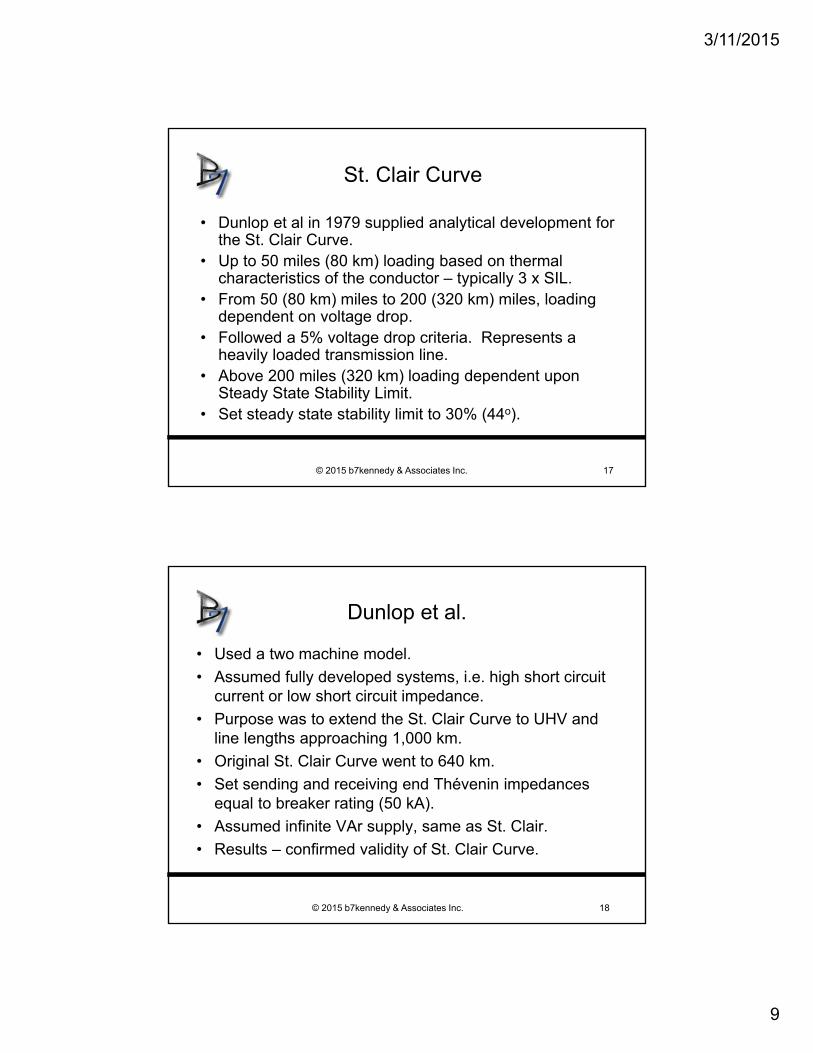
• Dunlop et al in 1979 supplied analytical development for the St. Clair Curve.
• Up to 50 miles (80 km) loading based on thermal characteristics of the conductor – typically 3 x SIL.
• From 50 (80 km) miles to 200 (320 km) miles, loading dependent on voltage drop.
• Followed a 5% voltage drop criteria. Represents a heavily loaded transmission line.
• Above 200 miles (320 km) loading dependent upon Steady State Stability Limit.
• Set steady state stability limit to 30% (44o).
© 2015 b7kennedy & Associates Inc. 17
Dunlop et al.
• Used a two machine model.
• Assumed fully developed systems, i.e. high short circuit current or low short circuit impedance.
• Purpose was to extend the St. Clair Curve to UHV and line lengths approaching 1,000 km.
• Original St. Clair Curve went to 640 km.
• Set sending and receiving end Thévenin impedances equal to breaker rating (50 kA).
• Assumed infinite VAr supply, same as St. Clair.
• Results – confirmed validity of St. Clair Curve.
© 2015 b7kennedy & Associates Inc. 18

3/11/2015
10
500 kV Example
• Red dotted line – trend line.
• For this example, smooth changeover between criteria.
• 500 kV short circuit level = 50 kA.
500 kV Line Loading
0.00
0.25
0.50
0.75
1.00
1.25
1.50
1.75
2.00
2.25
2.50
2.75
3.00
3.25
010
020
030
040
050
060
070
080
090
010
00
Length (km)
Lin
e L
oad
ing
(S
IL)
© 2015 b7kennedy & Associates Inc. 19
230 kV Example
• Red dotted line – trend line
• Demonstrates change over from voltage to angle criteria
• 240 kV system short circuit value = 20 kA
240 kV Line Loading
0.00
0.25
0.50
0.75
1.00
1.25
1.50
1.75
2.00
2.25
2.50
2.75
3.00
3.25
010
020
030
040
050
060
070
080
090
010
00
Distance (km)
Lin
e L
oad
ing
(S
IL)
© 2015 b7kennedy & Associates Inc. 20
3/11/2015
11
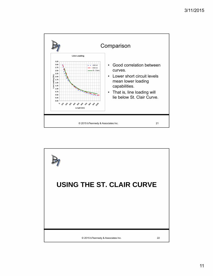
Comparison
• Good correlation between curves.
• Lower short circuit levels mean lower loading capabilities.
• That is, line loading will lie below St. Clair Curve.
Line Loading
0.00
0.25
0.50
0.75
1.00
1.25
1.50
1.75
2.00
2.25
2.50
2.75
3.00
3.25
010
020
030
040
050
060
070
080
090
010
00
Length (km)
Lin
e L
oad
ing
(S
IL)
240 kV
500 kV
St. Claire
© 2015 b7kennedy & Associates Inc. 21
USING THE ST. CLAIR CURVE
© 2015 b7kennedy & Associates Inc. 22

3/11/2015
12
Using St. Clair
• Need to supply a 100 MW load 125 km from the nearest source.
• Assume a simple power system, that is a two machine equivalent.
• What supply voltage do we pick?
• From St. Clair we see that at 125 km, we can transfer 2.25 times SIL.
• From the table of SIL: 100 MW is twice SIL at 138 kV and approximately 70% of SIL at 230 kV.
• The question now becomes – what reactive support does the new load require?
© 2015 b7kennedy & Associates Inc. 23
REACTIVE POWER FLOW
© 2015 b7kennedy & Associates Inc. 24

3/11/2015
13
Reactive Support
• At SIL, shunt capacitive energy equals series inductive energy.
• Below SIL there is an excess of shunt capacitive energy.
• Above SIL there is a deficiency of shunt capacitive energy.
• Sending and receiving ends have to supply the reactive energy.
© 2015 b7kennedy & Associates Inc. 25
Calculating Reactive Support
• Use the per unit (pu) system.• Define SIL = 1 pu & Voltage = 1 pu.• At SIL, current = 1 pu.• At 1.5 SIL, current equals 1.5 pu.• Series reactive energy = ½ LI2
• Required reactive energy = 2.25 pu.• Line supplies 1 pu.• Therefore required reactive energy =1.25 pu• Voltages are equal, therefore ½ VArs from each end.
© 2015 b7kennedy & Associates Inc. 26

3/11/2015
14
345 kV, 200 km Line Example
• From the table, charging is 605 kVAr/km• VArs at 1.5 SIL are:
200 x 0.605 x 1.52 = 272 MVAr• VArs @ SIL = 120 MVAr• Required VArs from each end = (272 – 120)/2
= 76 MVAr• Two machine model has the capability• Receiving end may require shunt capacitor bank,
depends on system planning and design considerations for a single machine model.
© 2015 b7kennedy & Associates Inc. 27
CONDUCTOR SELECTION
© 2015 b7kennedy & Associates Inc. 28

3/11/2015
15
Conductor Selection
• REA specifies minimum conductor sizes.• Larger conductors at higher voltages required to
minimize corona which is rich in harmonics.• Electric field at conductor surface is minimized with a
large conductor – larger surface area.• Bundling, i.e. using more than one conductor per phase
at higher voltages reduces onset of corona.• Allows use of two smaller conductors.
© 2015 b7kennedy & Associates Inc. 29
CONDUCTOR RATINGS
© 2015 b7kennedy & Associates Inc. 30

3/11/2015
16
Conductor Ratings
• IEEE 738-2012 defines rating of conductors.• Based on modified House & Tuttle method.• Four ratings – Summer, Winter, Operating and Thermal.• Summer Thermal – conductor 100oC, ambient 25oC, wind 2 fps.• Winter Thermal – conductor 100oC, ambient 0oC, wind 2 fps.• Operating limits, based on 75oC conductor temperature with the
same ambient conditions.• Ambient temperatures are location dependent and utility operating
experience.• Wind speed is fixed!• Rating includes orientation of the line, that is does it run north –
south or east – west.• In addition, latitude of the line is taken into account.
© 2015 b7kennedy & Associates Inc. 31
Transmission Line Conductor Ratings
© 2015 b7kennedy & Associates Inc. 32
Voltage (kV)
Conductor (MCM)
Summer Thermal
MVA
Winter Thermal
MVA
Summer Operating
MVA
Winter Operating
MVA
72 266 67 78 55 69
138 477 187 217 152 190
230 (single)
795 432 501 348 437
230 (bundled)
2x795 864 1002 697 874
345 (bundled)
3x795 1943 2255 1567 1968
500 (bundled)
4x795 3755 4358 30290 3802

3/11/2015
17
LOSSES
© 2015 b7kennedy & Associates Inc. 33
Transmission Losses
• Because the X/R ratio for higher voltage lines is in the vicinity of 10, we have been able to ignore losses.
• However, losses are always there.
• Losses vary in relation to the line loading.
• Transmission lines have a long life – 35 to 50 years.
• It’s important that the right conductor be chosen because the associated losses are paid every year.
• In addition, line loading is increasing every year.
© 2015 b7kennedy & Associates Inc. 34

3/11/2015
18
Transmission Losses
Transmission Losses
0
100
200
300
400
500
4750 5000 5250 5500 5750 6000 6250 6500 6750 7000 7250 7500 7750
Net Generation to Supply Alberta Load (MW)
Lo
sses
(M
W)
• Losses are variable or stochastic.
• Simple system – losses vary as a square of current.
• Complex system –losses display a linear variance.
© 2015 b7kennedy & Associates Inc. 35
Transmission Losses
Transmission Losses Histogram
0
100
200
300
400
500
197
210
223
236
249
262
275
288
301
314
327
340
353
366
379
392
405
418
431
Losses (MW)
Co
un
t
• Histogram demonstrates a normal distribution pattern for losses.
© 2015 b7kennedy & Associates Inc. 36

3/11/2015
19
Losses on a Simple System
• Take a radial 138 kV line and load it up.
• Losses vary as the square of the current times the resistance of the line.
138 kV Radial Line Losses
0
1
2
3
4
5
6
7
12.5 25.0 37.5 50.0 62.5 75.0 87.5 100.0 112.5 125.0 137.5 150.0
Loading (MW)
Lo
sses
(M
W)
© 2015 b7kennedy & Associates Inc. 37
ECONOMIC CONDUCTOR SELECTION
© 2015 b7kennedy & Associates Inc. 38

3/11/2015
20
Conductor Optimization
© 2015 b7kennedy & Associates Inc. 39
© 2015 b7kennedy & Associates Inc. 40

3/11/2015
21
VOLTAGE AND ANGLE
© 2015 b7kennedy & Associates Inc. 41
Voltage and Angle
• We know that active power is closely coupled to the angle between voltage sources.
• For this reason we can transfer large amounts of active power over great distances.
• We also know that reactive power is closely coupled to the difference in voltage magnitudes.
• However, the differences in voltage magnitudes is limited to 5%.
• As a result it’s not possible to transmit large amounts of reactive power over the power system.
• Reactive should generated and consumed where it’s needed.
© 2015 b7kennedy & Associates Inc. 42

3/11/2015
22
Voltage and Angle
© 2015 b7kennedy & Associates Inc. 43
slack
Sending END 423 MW
41 Mvar
Receiving END
2 6%A
MVA
1.05 pu 1.00 pu
-410 MW
-14 Mvar 26%A
MVA
Gen BusLoad Bus
0.00 Deg -21.70 Deg
Active Power
Reactive Powerangle
voltage
Voltage and Angle
© 2015 b7kennedy & Associates Inc. 44
• Voltage drop measured between line terminals and limited to 5%.
• Angle measured across whole system and includes short circuit impedances at sending and receiving ends and limited to 44o

3/11/2015
23
Sending and Receiving Voltages
• Use Vr as reference
• Load is at unity power factor
• Vr and I are in phase
• 230 kV, 175 km line• Load is 1½ SIL = 282 MW• Vr = 230/√3 = 133 kV• I = 282/(√3 x 230) = 0.708 kA• X = 175 x 0.4 = 70 Ω• IX = 0.708 x 70 = 49.6 kV• Vs = √(1332 + 49.62) • Vs = 142 kV• δ = tan-1 (49.6/133) = 20.5o
© 2015 b7kennedy & Associates Inc. 45
Line Angle
• What is the angle across a line or system?
• How do you calculate it?
• Use the telegraph or long line equations.
• Find α + jβ
• Attenuation constant = α
• Phase constant = jβ
• Phase constant is in radians/km.
• Convert to δ or degrees.
• Want a simpler method.
© 2015 b7kennedy & Associates Inc. 46

3/11/2015
24
Line Angle
• Want a short cut method for calculating the angle across a system or section of a system.
• In a 60 Hz system, the system goes through 21,600 degrees in 1 second.
• Energy travels across the system at the speed of light.
• The speed of light is 3x10⁵ km/sec.
• Therefore: system angle changes at 0.072 o/km.
• This is true at SIL of the system.
• Varies approximately in proportion to ratio of line loading to SIL.
© 2015 b7kennedy & Associates Inc. 47
Angle Across the Transmission Line
• Speed of light c = 3 x 10⁵ km/sec.
• In one second on a 60 Hz system 21,600o
• Dividing c into the degrees gives the constant 0.072o/km.
• Proportional to SIL.• δ = 0.072 x 175 x 1½ =
19oVr
Vs
• Interested in calculating the angle between Vs & Vr.
© 2015 b7kennedy & Associates Inc. 48

3/11/2015
25
MAXIMUM POWER TRANSFER
© 2015 b7kennedy & Associates Inc. 49
• P = Re (Es* I)
• Note: correct way is: P = Re (Es I*)
Maximum Power Transfer
© 2015 b7kennedy & Associates Inc. 50
3/11/2015
26
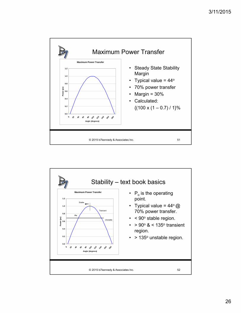
Maximum Power Transfer
• Steady State Stability Margin
• Typical value = 44o
• 70% power transfer
• Margin = 30%
• Calculated:
(100 x (1 – 0.7) / 1%
Maximum Power Transfer
0.0
0.2
0.4
0.6
0.8
1.0
1.2
0 20 40 60 80 100
120
140
160
180
Angle (degrees)
Po
wer
(p
u)
© 2015 b7kennedy & Associates Inc. 51
Stability – text book basics
• Po is the operating point.
• Typical value = 44o @ 70% power transfer.
• < 90o stable region.
• > 90o & < 135o transient region.
• > 135o unstable region.
Maximum Power Transfer
0.0
0.2
0.4
0.6
0.8
1.0
1.2
0 20 40 60 80 100
120
140
160
180
Angle (degrees)
Po
wer
(p
u)
Po
Stable
Transient
Unstable
© 2015 b7kennedy & Associates Inc. 52

3/11/2015
27
APPLICATION EXAMPLE
© 2015 b7kennedy & Associates Inc. 53
Application Example
• Let’s conclude with an application.
• You’re in the field, testing a 345 kV breaker.
• You’re finished for the day, and discover the 345 kV breaker won’t close.
• You trace the problem to the synchronizing check relay required for closing the breaker.
• What do you do?
© 2015 b7kennedy & Associates Inc. 54

3/11/2015
28
Ferranti Effect
• Open circuit voltage rise at the receiving end.• Can be worked out from first principles.• Travelling wave theory is best method.• Voltage rise equal to the inverse of the cosine of the
line angle.• Open end voltage rise on 230 kV, 250 km line is:
© 2015 b7kennedy & Associates Inc. 55
Synch Check
• Open 345 kV breaker won’t close.• Problem traced to Synch Check Relay – won’t
allow breaker to close.• Want to check the Synch Check Relay setting at
open breaker.
© 2015 b7kennedy & Associates Inc. 56

3/11/2015
29
Synch Check
• 345 kV parallel line 200 km in length each carrying SIL.
• With one line open, other line carries 2 SIL.• Angle is 29o.
© 2015 b7kennedy & Associates Inc. 57
Synch Check
• Design allows maximum voltage drop of 10%.
• Actual voltage drop is 12%.
• Open circuit voltage rise is 1.03 pu.
• Voltage difference across open breaker is 0.15 pu.
© 2015 b7kennedy & Associates Inc. 58
3/11/2015
30
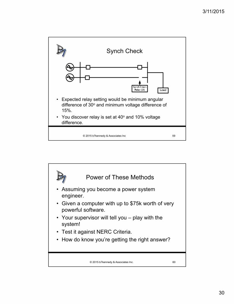
Synch Check
• Expected relay setting would be minimum angular difference of 30o and minimum voltage difference of 15%.
• You discover relay is set at 40o and 10% voltage difference.
© 2015 b7kennedy & Associates Inc 59
Power of These Methods
• Assuming you become a power system engineer.
• Given a computer with up to $75k worth of very powerful software.
• Your supervisor will tell you – play with the system!
• Test it against NERC Criteria.
• How do know you’re getting the right answer?
© 2015 b7kennedy & Associates Inc. 60

3/11/2015
31
NERC Requirements
• Category A – all facilities in service, system must be stable.
• That is no voltage violations and no equipment overloads.
• Category B – one piece of equipment out of service, system must be stable.
• Category C – two pieces out of service, system must be stable.
• Category D – three or more pieces out of service, load and or generator shedding, system must return to stable state.
© 2015 b7kennedy & Associates Inc. 61
Cautionary Note ...
• Understand these methods before you use them.
• Short cut methods are no substitute for detailed power flow and fault studies
• Can and should be used before you start your work!
• Can be used to validate your studies!• Develop your own numbers for the SIL table
as each power system is a little bit different.
© 2015 b7kennedy & Associates Inc. 62

3/11/2015
32
Transmission Line Summary
• Natural or SIL is an important property of transmission lines.
• SIL varies as the square of the line voltage.• St. Clair Curve shows loading is related to distance.• Overhead lines are most common for long distance
transmission.• Reactive power requirements vary as the loading of the
line.• Minimum conductor sizes dictated by corona.• Standards dictate maximum loading of conductor.• Transmission losses are fixed once conductor chosen.
© 2015 b7kennedy & Associates Inc. 63
That’s all folks!
• Discussion
• Questions
© 2015 b7kennedy & Associates Inc. 64