transport and fate of toxicants in the environment lieu tham khao chuong 3(1).… · transport and...

CHAPTER 27

Transport and Fate of Toxicantsin the Environment

DAMIAN SHEA

27.1 INTRODUCTION

More than 100,000 chemicals are released into the global environment every yearthrough their normal production, use, and disposal. To understand and predict thepotential risk that this environmental contamination poses to humans and wildlife,we must couple our knowledge on the toxicity of a chemical to our knowledge onhow chemicals enter into and behave in the environment. The simple box modelshown in Figure 27.1 illustrates the relationship between a toxicant source, its fatein the environment, its effective exposure or dose, and resulting biological effects. Aprospective or predictive assessment of a chemical hazard would begin by characteriz-ing the source of contamination, modeling the chemical’s fate to predict exposure, andusing exposure/dose-response functions to predict effects (moving from left to rightin Figure 27.1). A common application would be to assess the potential effects of anew waste discharge. A retrospective assessment would proceed in the opposite direc-tion starting with some observed effect and reconstructing events to find a probablecause. Assuming that we have reliable dose/exposure-response functions, the key tosuccessful use of this simple relationship is to develop a qualitative description andquantitative model of the sources and fate of toxicants in the environment.

Toxicants are released into the environment in many ways, and they can travelalong many pathways during their lifetime. A toxicant present in the environment ata given point in time and space can experience three possible outcomes: it can bestationary and add to the toxicant inventory and exposure at that location, it can betransported to another location, or it can be transformed into another chemical species.Environmental contamination and exposure resulting from the use of a chemical ismodified by the transport and transformation of the chemical in the environment.Dilution and degradation can attenuate the source emission, while processes that focusand accumulate the chemical can magnify the source emission. The actual fate ofa chemical depends on the chemical’s use pattern and physical-chemical properties,combined with the characteristics of the environment to which it is released.

A Textbook of Modern Toxicology, Third Edition, edited by Ernest HodgsonISBN 0-471-26508-X Copyright 2004 John Wiley & Sons, Inc.

479

Dr. Le Quoc Tuan

Rectangle

480 TRANSPORT AND FATE OF TOXICANTS IN THE ENVIRONMENT

Toxicant exposureToxicant source(s) Toxicant effects

Exposure–response modelTransport and fate model

Environmental factorsthat modify exposure

Figure 27.1 Environmental fate model. Such models are used to help determine how theenvironment modifies exposure resulting from various sources of toxicants.

Conceptually and mathematically, the transport and fate of a toxicant in the envi-ronment is very similar to that in a living organism. Toxicants can enter an organism orenvironmental system by many routes (e.g., dermal, oral, and inhalation versus smokestack, discharge pipe, or surface runoff). Toxicants are redistributed from their point ofentry by fluid dynamics (blood flow vs. water or air movement) and intermedia trans-port processes such as partitioning (blood-lipid partitioning vs. water-soil partitioning)and complexation (protein binding vs. binding to natural organic matter). Toxicants aretransformed in both humans and the environment to other chemicals by reactions suchas hydrolysis, oxidation, and reduction. Many enzymatic processes that detoxify andactivate chemicals in humans are very similar to microbial biotransformation pathwaysin the environment.

In fact, physiologically based pharmacokinetic models are similar to environmentalfate models. In both cases we divide a complicated system into simpler compart-ments, estimate the rate of transfer between the compartments, and estimate the rate oftransformation within each compartment. The obvious difference is that environmentalsystems are inherently much more complex because they have more routes of entry,more compartments, more variables (each with a greater range of values), and a lackof control over these variables for systematic study. The discussion that follows is ageneral overview of the transport and transformation of toxicants in the environmentin the context of developing qualitative and quantitative models of these processes.

27.2 SOURCES OF TOXICANTS TO THE ENVIRONMENT

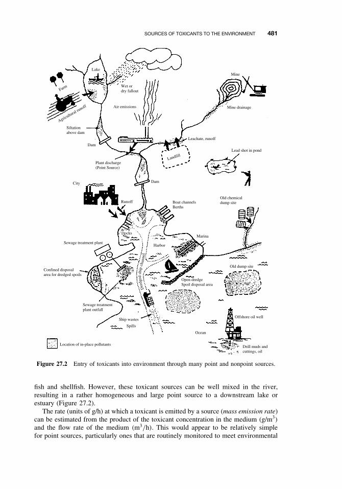
Environmental sources of toxicants can be categorized as either point sources or non-point sources (Figure 27.2). Point sources are discrete discharges of chemicals that areusually identifiable and measurable, such as industrial or municipal effluent outfalls,chemical or petroleum spills and dumps, smokestacks and other stationary atmosphericdischarges. Nonpoint sources are more diffuse inputs over large areas with no identifi-able single point of entry such as agrochemical (pesticide and fertilizer) runoff, mobilesources emissions (automobiles), atmospheric deposition, desorption or leaching fromvery large areas (contaminated sediments or mine tailings), and groundwater inflow.Nonpoint sources often include multiple smaller point sources, such as septic tanks orautomobiles, that are impractical to consider on an individual basis. Thus the identi-fication and characterization of a source is relative to the environmental compartmentor system being considered. For example, there may be dozens of important toxicantsources to a river, each must be considered when assessing the hazards of toxicantsto aquatic life in the river or to humans who might drink the water or consume the

SOURCES OF TOXICANTS TO THE ENVIRONMENT 481

Farm

Lake

Agricultural runoff

Wet ordry fallout

Air emissions

Dam

Dam

Siltationabove dam

Plant discharge(Point Source)

City

Runoff

Landfill

Leachate, runoff

Mine

Mine drainage

Lead shot in pond

Boat channelsBerths

Old chemicaldump site

Marina

Harbor

Docks

Open dredgeSpoil disposal area

Ocean

Offshore oil well

Old dump site

Drill muds andcuttings, oil

Location of in-place pollutants

Ship wastes

Spills

Confined disposalarea for dredged spoils

Sewage treatmentplant outfall

Sewage treatment plant

Dre

dged

ship

chan

nel

Figure 27.2 Entry of toxicants into environment through many point and nonpoint sources.

fish and shellfish. However, these toxicant sources can be well mixed in the river,resulting in a rather homogeneous and large point source to a downstream lake orestuary (Figure 27.2).

The rate (units of g/h) at which a toxicant is emitted by a source (mass emission rate)can be estimated from the product of the toxicant concentration in the medium (g/m3)

and the flow rate of the medium (m3/h). This would appear to be relatively simplefor point sources, particularly ones that are routinely monitored to meet environmental


regulations. However, the measurement of trace concentrations of chemicals in complexeffluent matrices is not a trivial task (see Chapter 25). Often the analytical methodsprescribed by environmental agencies for monitoring are not sensitive or selectiveenough to measure important toxicants or their reactive metabolites. Estimating themass emission rates for nonpoint sources is usually very difficult. For example, theatmospheric deposition of toxicants to a body of water can be highly dependent onboth space and time, and high annual loads can result from continuous depositionof trace concentrations that are difficult to measure. The loading of pesticides froman agricultural field to an adjacent body of water also varies with time and space asshown in Figure 27.3 for the herbicide atrazine. Rainfall following the application ofatrazine results in drainage ditch loadings more than 100-fold higher than just twoweeks following the rain. A much smaller, but longer lasting, increase in atrazineloading occurs at the edge of the field following the rain. Again, we see the needto define the spatial scale of concern when identifying and characterizing a source.If one is concerned with the fate of atrazine within a field, the source is defined bythe application rate. If one is concerned with the fate and exposure of atrazine in anadjacent body of water, the source may be defined as the drainage ditch and/or asrunoff from the edge of field. In the latter case one either needs to take appropriatemeasurements in the field or model the transport of atrazine from the field.

April May June July Aug Sept

2000

1500

1000

500

0

Large rain events

Period of atrazineapplication

Drainage ditch

Edge of field

Atr

azin

e co

ncen

trat

ion

(ng/

L)

Figure 27.3 Loading of atrazine from an agricultural field to an adjacent body of water. Theloading is highly dependent on rainfall and the presence of drainage ditches that collect thechemical and focus its movement in the environment.

TRANSPORT PROCESSES 483

27.3 TRANSPORT PROCESSES

Following the release of a toxicant into an environmental compartment, transport pro-cesses will determine its spatial and temporal distribution in the environment. Thetransport medium (or fluid) is usually either air or water, while the toxicant may bein dissolved, gaseous, condensed, or particulate phases. We can categorize physicaltransport as either advection or diffusion.

27.3.1 Advection

Advection is the passive movement of a chemical in bulk transport media either withinthe same medium (intraphase or homogeneous transport) or between different media(interphase or heterogeneous transport). Examples of homogeneous advection includetransport of a chemical in air on a windy day or a chemical dissolved in water moving ina flowing stream, in surface runoff (nonpoint source), or in a discharge effluent (pointsource). Examples of heterogeneous advection include the deposition of a toxicantsorbed to a suspended particle that settles to bottom sediments, atmospheric depositionto soil or water, and even ingestion of contaminated particles or food by an organism(i.e., bioaccumulation). Advection takes place independently from the presence of achemical; the chemical is simply going along for the ride. Advection is not influencedby diffusion and can transport a chemical either in the same or opposite direction asdiffusion. Thus advection is often called nondiffusive transport.

Homogeneous Advection. The homogeneous advective transport rate (N, g/h) issimply described in mathematical terms by the product of the chemical concentrationin the advecting medium (C, g/m3) and the flow rate of the medium (G, m3/h):

N = GC.

For example, if the flow of water out of a lake is 1000 m3/h and the concentration ofthe toxicant is 1 µg/m3, then the toxicant is being advected from the lake at a rate of1000 µg/h (or 1 mg/h). The emission rates for many toxicant sources can be calculatedin the same way.

As with source emissions, advection of air and water can vary substantially withtime and space within a given environmental compartment. Advection in a streamreach might be several orders of magnitude higher during a large rain event comparedto a prolonged dry period, while at one point in time, advection within a stagnantpool might be several orders of magnitude lower than a connected stream. Thus, aswith source characterization, we must match our estimates of advective transport tothe spatial and temporal scales of interest. Again, a good example is the movement ofatrazine from an agricultural field (Figure 27.3). Peak flow advective rates that followthe rain might be appropriate for assessing acute toxicity during peak flow periods butnot for estimating exposure at other times of the year. Conversely, an annual meanadvective rate would underestimate exposure during peak flow but would be moreappropriate for assessing chronic toxicity.

In surface waters advective currents often dominate the transport of toxicants, andthey can be estimated from hydrodynamic models or current measurements. In manycases advective flow can be approximated by the volume of water exchanged per unit


time by assuming conservation of mass and measuring flow into or out of the system.This works only for well mixed systems that have no or only small volumes of stagnantwater. In water bodies that experience density stratification (i.e., thermocline) separateadvective models or residence times can be used for each water layer. In air, advectionalso dominates the transport of chemicals, with air currents being driven by pressuregradients. The direction and magnitude of air velocities are recorded continuously inmany areas, and daily, seasonal, or annual means can be used to estimate advectiveair flow.

Advective air and water currents are much smaller in soil systems but still influencethe movement of chemicals that reside in soil. Advection of water in the saturatedzone is usually solved numerically from hydrodynamic models. Advection of air andwater in the unsaturated zone is complicated by the heterogeneity of these soil systems.Models are usually developed for specific soil property classes, and measurements ofthese soil properties are made at a specific site to determine which soil-model layersto link together.

Heterogeneous Advection. Heterogeneous advective transport involves a secondaryphase within the bulk advective phase, such as when a particle in air or water actsas a carrier of a chemical. In many cases we can treat heterogeneous advection thesame as homogeneous advection if we know the flow rate of the secondary phase andthe concentration of chemical in the secondary phase. In the lake example above, ifthe volume fraction of suspended particles in the lake water is 10−5, the flow rate ofsuspended particles is 0.01 m3/h, and the concentration of the toxicant in the solidparticles is 100 mg/m3, then the advective flow of the toxicant on suspended particleswill be 1 mg/h or the same as the homogeneous advection via water. Although the flowrate of particles is much lower than that of water, the concentration of the toxicant ismuch higher in the suspended particles than dissolved in the water. This is typical ofa hydrophobic toxicant such as DDT or benzo[a]pyrene. In soil and sedimentary sys-tems, colloidal particles (often macromolecular detritus) can play a very important rolein heterogeneous advective transport because they have greater mobility than largerparticles, and they often have greater capacity to sorb many toxicants because of theirhigher organic carbon content and higher surface area/mass ratio. In highly contami-nated sites, organic co-solvents can be present in the water (usually groundwater) andact as a high-capacity and high-efficiency carrier of toxicants through heterogeneousadvection in the water.

Unfortunately, the dynamics of heterogeneous transport are rarely simple, particu-larly over shorter scales of time and space. In addition to advection of particles withflowing water, aqueous phase heterogeneous transport includes particle settling, resus-pension, burial in bottom sediments, and mixing of bottom sediments. Particle settlingcan be an important mechanism for transporting hydrophobic toxicants from the waterto the bottom sediments. Modeling this process can be as simple as using an overallmass transfer coefficient or can include rigorous modeling of particles with differentsize, density, and organic carbon content. Estimates of particle settling are usuallyobtained through the use of laboratory settling chambers, in situ sediment traps, or bycalculation using Stoke’s law. Resuspension of bottom sediments occurs when suffi-cient energy is transferred to the sediment bed from advecting water, internal waves,boats, dredging, fishing, and the movement of sediment dwelling organisms (i.e., bio-turbation). Resuspension rates are difficult to measure and often are highly variable

TRANSPORT PROCESSES 485

in both time and space. Much as the annual runoff of pesticides from an agriculturalfield may be dominated by a few rain events, annual resuspension rates can be dom-inated by a major storm, and in smaller areas by a single boat or school of bottomfish. Resuspension rates can be estimated from sediment traps deployed just above thesediment surface or from the difference between particle settling and permanent burialor sedimentation. Sedimentation is the net result of particle settling and resuspensionand can be measured using radionuclide dating methods (e.g., 210Pb). Sediment dat-ing itself becomes difficult when there is significant mixing of the surface sediments(e.g., through bioturbation). Thus the heterogeneous transport of toxicants on aqueousparticles can be rather complicated, though many aquatic systems have been modeledreasonably well.

Heterogeneous advective transport in air occurs primarily through the absorption ofchemicals into falling water droplets (wet deposition) or the sorption of chemicals intosolid particles that fall to earth’s surface (dry deposition). Under certain conditionsboth processes can be treated as simple first-order advective transport using a flow rateand concentration in the advecting medium. For example, wet deposition is usuallycharacterized by a washout coefficient that is proportional to rainfall intensity.

27.3.2 Diffusion

Diffusion is the transport of a chemical by random motion due to a state of disequilib-rium. For example, diffusion causes the movement of a chemical within a phase (e.g.,water) from a location of relatively high concentration to a place of lower concentra-tion until the chemical is homogeneously distributed throughout the phase. Likewisediffusive transport will drive a chemical between media (e.g., water and air) until theirequilibrium concentrations are reached and thus the chemical potentials or fugacitiesare equal in each phase.

Diffusion within a Phase. Diffusional transport within a phase can result fromrandom (thermal) motion of the chemical (molecular diffusion), the random turbulentmixing of the transport medium (turbulent diffusion), or a combination of both. Tur-bulent diffusion usually dominates the diffusive (but not necessarily the advective)chemical transport in air and water due to the turbulent motions or eddies that arecommon in nature. In porous media (sediment and soil) the water velocities are typ-ically too low to create eddies, but random mixing still occurs as water tortuouslyflows around particles. This mechanical diffusion is often called dispersion by hydrol-ogists and dispersion on larger scales, such as when groundwater detours around largeareas of less permeable soil, is called macrodispersion. Note, however, that the termdispersion often is used by meteorologists and engineers to describe any turbulentdiffusion.

Although different physical mechanisms can cause diffusive mixing, they all causea net transport of a chemical from areas of higher concentration to areas of lowerconcentration. All diffusive processes are also referred to as Fickian transport becausethey all can be described mathematically by Fick’s first law, which states that the flow(or flux) of a chemical (N, g/h) is proportional to its concentration gradient (dC/dx):

N = −DA

(dC

dx

),


where D is the diffusivity or mass transfer coefficient (m2/h), A is the area throughwhich the chemical is passing (m2), C is the concentration of the diffusing chemical(g/m3), and x is the distance being considered (m). The negative sign is simply theconvention that the direction of diffusion is from high to low concentration (diffusion ispositive when dC/dx is negative). Note that many scientists and texts define diffusionas an area specific process with units of g/m2h and thus the area term (A) is not includedin the diffusion equation. This is simply an alternative designation that describes trans-port as a flux density (g/m2h) rather than as a flow (g/h). In either case the diffusionequation can be integrated numerically and even expressed in three dimensions usingvector notation. However, for most environmental situations we usually have no accu-rate estimate of D or dx, so we combine the two into a one-dimensional mass transfercoefficient (kM) with units of velocity (m/h). The chemical flux is then the product ofthis velocity, area, and concentration:

N = −kMAC.

Mass transfer coefficients can be estimated from laboratory, mesocosm, and fieldstudies and are widely used in environmental fate models. Mass transfer coefficientscan be derived separately for molecular diffusion, turbulent diffusion, and dispersionin porous media, and all three terms can be added to the chemical flux equation.This is usually not necessary because one term often dominates the transport in spe-cific environmental regions. Consider the vertical diffusion of methane gas generatedby methanogenic bacteria in deep sediments. Molecular diffusion dominates in thehighly compacted and low porosity deeper sediments. Dispersion becomes importantas methane approaches the more porous surface sediments. Following methane gasebulation from the sediment porewater, turbulent diffusion will dominate transport ina well-mixed water column (i.e., not a stagnant pool or beneath a thermocline wheremolecular diffusion will dominate). At the water surface, eddies tend to be dampedand molecular diffusion may again dominate transport. Under stagnant atmosphericconditions (i.e., a temperature inversion) molecular diffusion will continue to dominatebut will yield to more rapid mixing when typical turbulent conditions are reached. Themagnitude and variability of the transport rate generally increase as the methane movesvertically through the environment, except when very stagnant conditions are encoun-tered in the water or air. Modeling the transport of a chemical in air is particularlydifficult because of the high spatial and temporal variability of air movement. Notealso that advective processes in water or air usually transport chemicals at a faster ratethan either molecular or turbulent diffusion.

Diffusion between Phases. The transport of a chemical between phases is some-times treated as a third category of transport processes or even as a transformationreaction. Interphase or intermedia transport is not a transformation reaction becausethe chemical is moving only between phases; it is not reacting with anything or chang-ing its chemical structure. Instead, intermedia transport is simply driven by diffusionbetween two phases. When a chemical reaches an interface such as air–water, parti-cle–water, or (biological) membrane–water, two diffusive regions are created at eitherside of the interface. The classical description of this process is the Whitman two-filmor two-resistance mass transfer theory, where chemicals pass through two stagnantboundary layers by molecular diffusion, while the two bulk phases are assumed to

EQUILIBRIUM PARTITIONING 487

be homogeneously mixed. This allows us to use a first-order function of the concen-tration gradient in the two phases, where the mass transfer coefficient will dependonly on the molecular diffusivity of the chemical in each phase and the thickness ofthe boundary layers. This is fairly straightforward for transfer at the air–water inter-face (and often at the membrane–water interface), but not for the particle–water orparticle–air interfaces.

Diffusive transport between phases can be described mathematically as the productof the departure from equilibrium and a kinetic term:

N = kA(C1 − C2K12),

where N is the transport rate (g/h), k is a transport rate coefficient (m/h), A is theinterfacial area (m2), C1 and C2 are the concentrations in the two phases, and K12 is theequilibrium partition coefficient. At equilibrium K12 equals C1/C2, the term describingthe departure from equilibrium (C1 − C2K12) becomes zero, and thus the net rate oftransfer also is zero. The partition coefficients are readily obtained from thermodynamicdata and equilibrium partitioning experiments. The transport rate coefficients are usuallyestimated from the transport rate equation itself by measuring intermedia transport rates(N ) under controlled laboratory conditions (temperature, wind and water velocities) atknown values of A, C1, C2, and K12. These measurements must then be extrapolated tothe field, sometimes with great uncertainty. This uncertainty, along with the knowledgethat many interfacial regions have reached or are near equilibrium, has led many tosimply assume that equilibrium exists at the interface. Thus the net transport rate iszero and the phase distribution of a chemical is simply described by its equilibriumpartition coefficient.

27.4 EQUILIBRIUM PARTITIONING

When a small amount of a chemical is added to two immiscible phases and then shaken,the phases will eventually separate and the chemical will partition between the twophases according to its solubility in each phase. The concentration ratio at equilibriumis the partition coefficient:

C1

C2= K12.

In the laboratory, we usually determine K12 from the slope of C1 versus C2 overa range of concentrations. Partition coefficients can be measured for essentially anytwo-phase system: air–water, octanol–water, lipid–water, particle–water, and so on.In situ partition coefficients also can be measured where site-specific environmentalconditions might influence the equilibrium phase distribution.

27.4.1 Air–Water Partitioning

Air–water partition coefficients (Kair−water) are essentially Henry’s law constants (H ):

Kair−water = H = Cair

Cwater,


where H can be expressed in dimensionless form (same units for air and water) orin units of pressure divided by concentration (e.g., Pa m3/mol). The latter is usuallywritten as

H = Pair

Cwater,

where Pair is the partial vapor pressure of the chemical. When H is not measureddirectly, it can be estimated from the ratio of the chemical’s vapor pressure and aqueoussolubility, although one must be careful about using vapor pressures and solubilities thatapply to the same temperature and phase. Chemicals with high Henry’s law constants(e.g., alkanes and many chlorinated solvents) have a tendency to escape from water toair and typically have high vapor pressures, low aqueous solubilities, and low boilingpoints. Chemicals with low Henry’s law constants (e.g., alcohols, chlorinated phenols,larger polycyclic aromatic hydrocarbons, lindane, atrazine) tend to have high watersolubility and/or very low vapor pressure. Note that some chemicals that are consideredto be “nonvolatile,” such as DDT, are often assumed to have low Henry’s law constants.However, DDT also has a very low water solubility yielding a rather high Henry’s lawconstant. Thus DDT readily partitions into the atmosphere as is now apparent from theglobal distribution of DDT.

27.4.2 Octanol–Water Partitioning

For many decades chemists have been measuring the octanol–water partition coeffi-cient (KOW) as a descriptor of hydrophobicity or how much a chemical “hates” to bein water. It is now one of the most important and frequently used physicochemicalproperties in toxicology and environmental chemistry. In fact toxicologists often sim-ply use the symbol P , for partition coefficient, as if no other partition coefficient isimportant. Strong correlations exist between KOW and many biochemical and toxico-logical properties. Octanol has a similar carbon:oxygen ratio as lipids, and the KOW

correlates particularly well with lipid–water partition coefficients. This has led many touse KOW as a measure of lipophilicity or how much a chemical “loves” lipids. This isreally not the case because most chemicals have an equal affinity for octanol and otherlipids (within about a factor of ten), but their affinity for water varies by many ordersof magnitude. Thus it is largely aqueous solubility which determines KOW not octanolor lipid solubility. We generally express KOW as log KOW because KOW values rangefrom less than one (alcohols) to over one billion (larger alkanes and alkyl benzenes).

27.4.3 Lipid–Water Partitioning

In most cases we can assume that the equilibrium distribution and partitioning oforganic chemicals in both mammalian and nonmammalian systems is a function oflipid content in the animal and that the lipid–water partition coefficient (KLW) isequal to KOW. Instances where this is not the case include specific binding sites (e.g.,kepone in the liver) and nonequilibrium conditions caused by slow elimination ratesof higher level organisms or structured lipid phases that sterically hinder accumulationof very hydrophobic chemicals. For aquatic organisms in constant contact with water,the bioconcentration factor or fish-water partition coefficient (KFW) is simply:

KFW = flipidKOW,

EQUILIBRIUM PARTITIONING 489

where flipid is the mass fraction of lipid in the fish (g lipid/g fish). Several studies haveshown this relationship works well for many fish and shellfish species and an aggregateplot of KFW versus KOW for many different fish species yields a slope of 0.048, whichis about the average lipid concentration of fish (5%). Again, nonequilibrium conditionswill cause deviation from this equation. Such deviations are found at both the top andbottom of the aquatic food chain. Phytoplankton can have higher apparent lipid–waterpartition coefficients because their large surface area : volume ratios increase the rela-tive importance of surface sorption. Top predators such as marine mammals also havehigh apparent lipid-water partition coefficients because of very slow elimination rates.Thus the deviations occur not because “there is something wrong with the equation”but because the underlying assumption of equilibrium is not appropriate in these cases.

27.4.4 Particle–Water Partitioning

It has been known for several decades that many chemicals preferentially associatewith soil and sediment particles rather than the aqueous phase. The particle–waterpartition coefficient (KP) describing this phenomenon is

KP = CS

CW,

where CS is the concentration of chemical in the soil or sediment (mg/kg dry weight)and CW is the concentration in water (mg/L). In this form, KP has units of L/kgor reciprocal density. Dimensionless partition coefficients are sometimes used whereKP is multiplied by the particle density (in kg/L). It has also been observed, first bypesticide chemists in soil systems and later by environmental engineers and chemists insewage effluent and sediment systems, that nonionic organic chemicals were primarilyassociated with the organic carbon phase(s) of particles. A plot of KP versus the massfraction of organic carbon in the soil (fOC, g/g) is linear with a near-zero interceptyielding the simple relationship

KP = fOCKOC,

where KOC is the organic carbon–water partition coefficient (L/kg). Studies withmany chemicals and many sediment/soil systems have demonstrated the utility of thisequation when the fraction of organic carbon is about 0.5% or greater. At lower organiccarbon fractions, interaction with the mineral phase becomes relatively more important(though highly variable) resulting in a small positive intercept of KP versus fOC. Thestrongest interaction between organic chemicals and mineral phases appears to be withdry clays. Thus KP will likely change substantially as a function of water content inlow organic carbon, clay soils.

Measurements of KOC have been taken directly from partitioning experiments insediment–and soil–water systems over a range of environmental conditions in both thelaboratory and the field. Not surprisingly, the KOC values for many organic chemicalsare highly correlated with their KOW values. Plots of the two partition coefficients forhundreds of chemicals with widely ranging KOW values yield slopes from about 0.3 to1, depending on the classes of compounds and the particular methods included. Mostfate modelers continue to use a slope of 0.41, which was reported by the first definitive


study on the subject in the early 1980s. Thus we now have a means of estimating thepartitioning of a chemical between a particle and water by using the KOW and fOC:

KP = fOCKOC = fOC 0.41KOW.

This relationship is commonly used in environmental fate models to predict aqueousconcentrations from sediment measurements by substituting the equilibrium expressionfor KP and rearranging to solve for CW:

KP = CS

CW= fOC 0.41KOW,

CW = CS

fOC0.41KOW.

This last equation forms the basis for the EPA’s sediment quality guidelines that areused to assess the potential toxicity of contaminated sediments. The idea is to simplymeasure CS and fOC, look up KOW in a table, compute the predicted CW, and comparethis result to established water quality criteria for the protection of aquatic life or humanlife (e.g., carcinogenicity risk factors). The use of this simple equilibrium partitioningexpression for this purpose is currently the subject of much debate among scientists aswell as policy makers.

27.5 TRANSFORMATION PROCESSES

The potential environmental hazard associated with the use of a chemical is directlyrelated to it’s persistence in the environment (see Chapter 26), which in turn dependson the rates of chemical transformation reactions. Transformation reactions can bedivided into two classes: reversible reactions that involve continuous exchange amongchemical states (ionization, complexation) and irreversible reactions that permanentlytransform a parent chemical into a daughter or reaction product (photolysis, hydrolysis,and many redox reactions). Reversible reactions are usually abiotic, although biologicalprocesses can still exert great influence over them (e.g., via production of complexingagents or a change in pH). Irreversible reactions can be abiotic or mediated directlyby biota, particularly bacteria.

27.5.1 Reversible Reactions

Ionization. Ionization refers to the dissociation of a neutral chemical into chargedspecies. The most common form of neutral toxicant dissociation is acid-base equilibria.The hypothetical monoprotic acid, HA, will dissociate in water to form the conjugateacid-base pair (H+, A−) usually written as

HA + H2O = H3O+ + A−.

The equilibrium constant for this reaction, the acidity constant (Ka), is defined by thelaw of mass action and is given by

Ka = [H3O+][A−]

[HA].

TRANSFORMATION PROCESSES 491

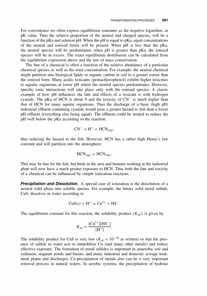
For convenience we often express equilibrium constants as the negative logarithm, orpK value. Thus the relative proportion of the neutral and charged species, will be afunction of the pKa and solution pH. When the pH is equal to pKa, equal concentrationsof the neutral and ionized forms will be present. When pH is less than the pKa,the neutral species will be predominant; when pH is greater than pKa, the ionizedspecies will be in excess. The exact equilibrium distribution can be calculated fromthe equilibrium expression above and the law of mass conservation.

The fate of a chemical is often a function of the relative abundance of a particularchemical species as well as the total concentration. For example, the neutral chemicalmight partition into biological lipids or organic carbon in soil to a greater extent thanthe ionized form. Many acidic toxicants (pentachlorophenol) exhibit higher toxicitiesto aquatic organisms at lower pH where the neutral species predominates. However,specific ionic interactions will take place only with the ionized species. A classicexample of how pH influences the fate and effects of a toxicant is with hydrogencyanide. The pKa of HCN is about 9 and the toxicity of CN− is much higher thanthat of HCN for many aquatic organisms. Thus the discharge of a basic (high pH)industrial effluent containing cyanide would pose a greater hazard to fish than a lowerpH effluent (everything else being equal). The effluent could be treated to reduce thepH well below the pKa according to the reaction:

CN− + H+ = HCN(aq),

thus reducing the hazard to the fish. However, HCN has a rather high Henry’s lawconstant and will partition into the atmosphere:

HCN(aq) = HCN(air).

This may be fine for the fish, but birds in the area and humans working at the industrialplant will now have a much greater exposure to HCN. Thus both the fate and toxicityof a chemical can be influenced by simple ionization reactions.

Precipitation and Dissolution. A special case of ionization is the dissolution of aneutral solid phase into soluble species. For example, the binary solid metal sulfide,CuS, dissolves in water according to

CuS(s) + H+ = Cu2+ + HS−.

The equilibrium constant for this reaction, the solubility product (Ksp), is given by

Ksp = [Cu2+][HS−]

[H+].

The solubility product for CuS is very low (Ksp = 10−19 as written) so that the pres-ence of sulfide in water acts to immobilize Cu (and many other metals) and reduceeffective exposure. The formation of metal sulfides is important in anaerobic soil andsediment, stagnant ponds and basins, and many industrial and domestic sewage treat-ment plants and discharges. Co-precipitation of metals also can be a very importantremoval process in natural waters. In aerobic systems, the precipitation of hydrous


oxides of manganese and iron often incorporate other metals as impurities. In anaero-bic systems, the precipitation of iron sulfides can include other metals as well. Theseco-precipitates are usually not thermodynamically stable, but their conversion to stablemineral phases often takes place on geological time scales.

Complexation and Chemical Speciation. Natural systems contain many chemicalsthat undergo ionic or covalent interactions with toxicants to change toxicant specia-tion and chemical speciation can have a profound effect on both fate and toxicity.Again, in the case of copper, inorganic ions (Cl−, OH−) and organic detritus (humicacids, peptides) will react with dissolved Cu2+ to form various metal-ligand com-plexes. Molecular diffusivities of complexed copper will be lower than uncomplexed(hydrated) copper and will generally decrease with the size and number of ligands.The toxicity of free, uncomplexed Cu2+ to many aquatic organisms is much higherthan Cu2+ that is complexed to chelating agents such as EDTA or glutathione. Manytransition metal toxicants, such as Cu, Pb, Cd, and Hg, have high binding constantswith compounds that contain amine, sulfhydryl, and carboxylic acid groups. Thesegroups are quite common in natural organic matter. Even inorganic complexes of OH−and Cl− reduce Cu2+ toxicity. In systems where a mineral phase is controlling Cu2+solubility, the addition of these complexing agents will shift the solubility equilibriumaccording to LeChatelier’s principle as shown here for CuS and OH−, Cl−, and GSH(glutathione):

CuS(s) + H+ = Cu2+ + HS−, Ksp,

Cu2+ + OH− = CuOH+, KCuOH,

Cu2+ + Cl− = CuCl+, KCuCl,

Cu2+ + GSH = CuGS+ + H+, KCuGS.

Each successive complexation reaction “leaches” Cu2+ from the solid mineral phase,thereby increasing the total copper in the water but not affecting the concentration of(or exposure to) Cu2+. These equilibria can be combined into one reaction:

4CuS(s) + 3H+ + OH− + Cl− + GSH = Cu2+ + 4HS−

+ CuOH+ + CuCl+ + CuGS+,

and the overall equilibrium constant derived as shown:

Koverall = (4)Ksp × KCuOH × KCuCl × KCuGS

= [Cu2+] [CuOH+] [CuCl+] [CuGS+] [HS−]4/[H+]3 [OH−] [Cl−] [GS−].

A series of simultaneous equations can be derived for these reactions to computethe concentration of individual copper species, and the total concentration of copper,[Cu]T, would be given by

[Cu]T = [Cu2+] + [CuOH+] + [CuCl+] + [CuGS+].

Thus the total copper added to a toxicity test or measured as the exposure (e.g., byatomic absorption spectroscopy) may be much greater than that which is available toan organism to induce toxicological effects.


Literally hundreds of complex equilibria like this can be combined to model whathappens to metals in aqueous systems. Numerous speciation models exist for this appli-cation that include all of the necessary equilibrium constants. Several of these modelsinclude surface complexation reactions that take place at the particle–water interface.Unlike the partitioning of hydrophobic organic contaminants into organic carbon, met-als actually form ionic and covalent bonds with surface ligands such as sulfhydrylgroups on metal sulfides and oxide groups on the hydrous oxides of manganese andiron. Metals also can be biotransformed to more toxic species (e.g., conversion of ele-mental mercury to methyl-mercury by anaerobic bacteria), less toxic species (oxidationof tributyl tin to elemental tin), or temporarily immobilized (e.g., via microbial reduc-tion of sulfate to sulfide, which then precipitates as an insoluble metal sulfide mineral).

27.5.2 Irreversible Reactions

The reversible transformation reactions discussed above alter the fate and toxicityof chemicals, but they do not irreversibly change the structure or properties of thechemical. An acid can be neutralized to its conjugate base, and vice versa. Copper canprecipitate as a metal sulfide, dissolve and from a complex with numerous ligands,and later re-precipitate as a metal sulfide. Irreversible transformation reactions alterthe structure and properties of a chemical forever.

Hydrolysis. Hydrolysis is the cleavage of organic molecules by reaction with waterwith a net displacement of a leaving group (X) with OH−:

RX + H2O = ROH + HX.

Hydrolysis is part of the larger class of chemical reactions called nucleophilic displace-ment reactions in which a nucleophile (electron-rich species with an unshared pair ofelectrons) attacks an electrophile (electron deficient), cleaving one covalent bond toform a new one. Hydrolysis is usually associated with surface waters but also takesplace in the atmosphere (fogs and clouds), groundwater, at the particle–water interfaceof soils and sediments, and in living organisms.

Hydrolysis can proceed through numerous mechanisms via attack by H2O (neutralhydrolysis) or by acid (H+) or base (OH−) catalysis. Acid and base catalyzed reactionsproceed via alternative mechanisms that require less energy than neutral hydrolysis.The combined hydrolysis rate term is a sum of these three constituent reactions and isgiven by

d[RX]

dt= kobs[RX] = ka[H+][RX] + kn[RX] + kb[OH−][RX],

where [RX] is the concentration of the hydrolyzable chemical, kobs is the macroscopicobserved hydrolysis rate constant, and ka, kn, and kb are the rate constants for the acid-catalyzed, neutral, and base-catalyzed hydrolysis. If we assume that the hydrolysis canbe approximated by first-order kinetics with respect to RX (which is usually true), therate term is reduced to

kobs = ka[H+] + kn + kb[OH−].

Neutral hydrolysis is dependent only on water which is present in excess, so kn is asimple pseudo-first-order rate constant (with units t−1). The acid- and base-catalyzed


hydrolysis depend on the molar quantities of [H+] and [OH−], respectively, so ka andkb have units of M−1t−1.

The observed or apparent hydrolysis half-life at a fixed pH is then given by

t1/2 = ln 2

kobs.

Compilations of hydrolysis half-lives at pH and temperature ranges encountered innature can be found in many sources. Reported hydrolysis half-lives for organic com-pounds at pH 7 and 298 K range at least 13 orders of magnitude. Many esters hydrolyzewithin hours or days, whereas some organic chemicals will never hydrolyze. For halo-genated methanes, which are common groundwater contaminants, half-lives range fromabout 1 year for CH3Cl to about 7000 years for CCl4. The half-lives of halomethanesfollows the strength of the carbon-halogen bond with half-lives decreasing in theorder F > Cl > Br. Small structural changes can dramatically alter hydrolysis rates.An example is the difference between tetrachloroethane (Cl2HC–CHCl2) and tetra-chloroethene (Cl2C=CCl2) which have hydrolysis half-lives of about 0.5 year and109 years, respectively. In this case the hydrolysis rate is affected by the C–Cl bondstrength and the steric bulk at the site of nucleophilic substitution.

The apparent rate of hydrolysis and the relative abundance of reaction products isoften a function of pH because alternative reaction pathways are preferred at differentpH. In the case of halogenated hydrocarbons, base-catalyzed hydrolysis will result inelimination reactions while neutral hydrolysis will take place via nucleophilic displace-ment reactions. An example of the pH dependence of hydrolysis is illustrated by thebase-catalyzed hydrolysis of the structurally similar insecticides DDT and methoxy-chlor. Under a common range of natural pH (5 to 8) the hydrolysis rate of methoxychloris invariant while the hydrolysis of DDT is about 15-fold faster at pH 8 compared topH 5. Only at higher pH (>8) does the hydrolysis rate of methoxychlor increase. Inaddition the major product of DDT hydrolysis throughout this pH range is the same(DDE), while the methoxychlor hydrolysis product shifts from the alcohol at pH 5–8(nucleophilic substitution) to the dehydrochlorinated DMDE at pH > 8 (elimination).This illustrates the necessity to conduct detailed mechanistic experiments as a functionof pH for hydrolytic reactions.

Photolysis. Photolysis of a chemical can proceed either by direct absorption of light(direct photolysis) or by reaction with another chemical species that has been producedor excited by light (indirect photolysis). In either case photochemical transformationssuch as bond cleavage, isomerization, intramolecular rearrangement, and various inter-molecular reactions can result. Photolysis can take place wherever sufficient lightenergy exists, including the atmosphere (in the gas phase and in aerosols and fog/clouddroplets), surface waters (in the dissolved phase or at the particle–water interface), andin the terrestrial environment (on plant and soil/mineral surfaces).

Photolysis dominates the fate of many chemicals in the atmosphere because of thehigh solar irradiance. Near the earth’s surface, chromophores such as nitrogen oxides,carbonyls, and aromatic hydrocarbons play a large role in contaminant fate in urbanareas. In the stratosphere, light is absorbed by ozone, oxygen, organohalogens, andhydrocarbons with global environmental implications. The rate of photolysis in surfacewaters depends on light intensity at the air–water interface, the transmittance through


this interface, and the attenuation through the water column. Open ocean waters (“bluewater”) can transmit blue light to depths of 150 m while highly eutrophic or turbidwaters might absorb all light within 1 cm of the surface.

Oxidation-Reduction Reactions. Although many redox reactions are reversible,they are included here because many of the redox reactions that influence the fateof toxicants are irreversible on the temporal and spatial scales that are importantto toxicity.

Oxidation is simply defined as a loss of electrons. Oxidizing agents are electrophilesand thus gain electrons upon reaction. Oxidations can result in the increase in the oxi-dation state of the chemical as in the oxidation of metals or oxidation can incorporateoxygen into the molecule. Typical organic chemical oxidative reactions include dealky-lation, epoxidation, aromatic ring cleavage, and hydroxylation. The term autooxidation,or weathering, is commonly used to describe the general oxidative degradation of achemical (or chemical mixture, e.g., petroleum) upon exposure to air. Chemicals canreact abiotically in both water and air with oxygen, ozone, peroxides, free radicals,and singlet oxygen. The last two are common intermediate reactants in indirect pho-tolysis. Mineral surfaces are known to catalyze many oxidative reactions. Clays andoxides of silicon, aluminum, iron, and manganese can provide surface active sites thatincrease rates of oxidation. There are a variety of complex mechanisms associated withthis catalysis, so it is difficult to predict the catalytic activity of soils and sedimentin nature.

Reduction of a chemical species takes place when an electron donor (reductant)transfers electrons to an electron acceptor (oxidant). Organic chemicals typically actas the oxidant, while abiotic reductants include sulfide minerals, reduced metals orsulfur compounds, and natural organic matter. There are also extracellular biochemicalreducing agents such as porphyrins, corrinoids, and metal-containing coenzymes. Mostof these reducing agents are present only in anaerobic environments where anaero-bic bacteria are themselves busy reducing chemicals. Thus it is usually very difficultto distinguish biotic and abiotic reductive processes in nature. Well-controlled, sterilelaboratory studies are required to measure abiotic rates of reduction. These studies indi-cate that many abiotic reductive transformations could be important in the environment,including dehalogenation, dealkylation, and the reduction of quinones, nitrosamines,azoaromatics, nitroaromatics, and sulfoxides. Functional groups that are resistant toreduction include aldehydes, ketones, carboxylic acids (and esters), amides, alkenes,and aromatic hydrocarbons.

Biotransformations. As we have seen throughout much of this textbook, verte-brates have developed the capacity to transform many toxicants into other chemicals,sometimes detoxifying the chemical and sometimes activating it. The same or simi-lar biochemical processes that hydrolyze, oxidize, and reduce toxicants in vertebratesalso take place in many lower organisms. In particular, bacteria, protozoans, and fungiprovide a significant capacity to biotransform toxicants in the environment. Althoughmany vertebrates can metabolize toxicants faster than these lower forms of life, theaggregate capacity of vertebrates to biotransform toxicants (based on total biomass andexposure) is insignificant to the overall fate of a toxicant in the environment. In thissection we use the term biotransformation to include all forms of direct biologicaltransformation reactions.


Biotransformations follow a complex series of chemical reactions that are enzymat-ically mediated and are usually irreversible reactions that are energetically favorable,resulting in a decrease in the Gibbs free energy of the system. Thus the potential forbiotransformation of a chemical depends on the reduction in free energy that resultsfrom reacting the chemical with other chemicals in its environment (e.g., oxygen). Aswith inorganic catalysts, microbes simply use enzymes to lower the activation energyof the reaction and increase the rate of the transformation. Each successive chemicalreaction further degrades the chemical, eventually mineralizing it to inorganic com-pounds (CO2, H2O, inorganic salts) and continuing the carbon and hydrologic cycleson earth.

Usually microbial growth is stimulated because the microbes capture the energyreleased from the biotransformation reaction. As the microbial population expands,overall biotransformation rates increase, even though the rate for each individualmicrobe may be constant or even decrease. This complicates the modeling and pre-diction of biotransformation rates in nature. When the toxicant concentrations (andpotential energy) are small relative to other substrates or when the microbes cannotefficiently capture the energy from the biotransformation, microbial growth is not stim-ulated but biotransformation often still proceeds inadvertently through cometabolism.

Biotransformation can be modeled using simple Michaelis-Menten enzyme kinetics,Monod microbial growth kinetics, or more complex numerical models that incorpo-rate various environmental parameters, and even the formation of microbial mats orslime, which affects diffusion of the chemical and nutrients to the microbial population.Microbial ecology involves a complex web of interaction among numerous environ-mental processes and parameters. The viability of microbial populations and the ratesof biotransformation depend on many factors such as genetic adaptation, moisture,nutrients, oxygen, pH, and temperature. Although a single factor may limit biotrans-formation rates at a particular time and location, we cannot generalize about what limitsbiotransformation rates in the environment. Biotransformation rates often increase withtemperature (according to the Arrhenius law) within the optimum range that supportsthe microbes, but many exceptions exist for certain organisms and chemicals. Theavailability of oxygen and various nutrients (C, N, P, Fe, Si) often limits microbialgrowth, but the limiting nutrient often changes with space (e.g., downriver) and time(seasonally and even diurnally).

Long-term exposure of microbial populations to certain toxicants often is necessaryfor adaptation of enzymatic systems capable of degrading those toxicants. This wasthe case with the Exxon Valdez oil spill in Alaska in 1989. Natural microbial popu-lations in Prince William Sound, Alaska, had developed enzyme systems that oxidizepetroleum hydrocarbons because of long-term exposure to natural oil seeps and tohydrocarbons that leached from the pine forests in the area. Growth of these naturalmicrobial populations was nutrient limited during the summer. Thus the applicationof nutrient formulations to the rocky beaches of Prince William Sound stimulatedmicrobial growth and helped to degrade the spilled oil.

In terrestrial systems with high nutrient and oxygen content, low moisture and highorganic carbon can control biotransformation by limiting microbial growth and theavailability of the toxicant to the microbes. For example, biotransformation rates ofcertain pesticides have been shown to vary two orders of magnitude in two sepa-rate agricultural fields that were both well aerated and nutrient rich, but spanned thecommon range of moisture and organic carbon content.

ENVIRONMENTAL FATE MODELS 497

27.6 ENVIRONMENTAL FATE MODELS

The discussion above provides a brief qualitative introduction to the transport and fateof chemicals in the environment. The goal of most fate chemists and engineers is totranslate this qualitative picture into a conceptual model and ultimately into a quanti-tative description that can be used to predict or reconstruct the fate of a chemical inthe environment (Figure 27.1). This quantitative description usually takes the form ofa mass balance model. The idea is to compartmentalize the environment into definedunits (control volumes) and to write a mathematical expression for the mass balancewithin the compartment. As with pharmacokinetic models, transfer between compart-ments can be included as the complexity of the model increases. There is a great dealof subjectivity to assembling a mass balance model. However, each decision to includeor exclude a process or compartment is based on one or more assumptions—most ofwhich can be tested at some level. Over time the applicability of various assump-tions for particular chemicals and environmental conditions become known and modelstandardization becomes possible.

The construction of a mass balance model follows the general outline of this chapter.First, one defines the spatial and temporal scales to be considered and establishesthe environmental compartments or control volumes. Second, the source emissionsare identified and quantified. Third, the mathematical expressions for advective anddiffusive transport processes are written. And last, chemical transformation processesare quantified. This model-building process is illustrated in Figure 27.4. In this examplewe simply equate the change in chemical inventory (total mass in the system) withthe difference between chemical inputs and outputs to the system. The inputs couldinclude numerous point and nonpoint sources or could be a single estimate of totalchemical load to the system. The outputs include all of the loss mechanisms: transport

Atmosphericdeposition, Iair

Advective inputfrom river, Iriver

Diffusion toatomosphere, Oair

Homogeneousadvection, Odissolved

Heterogeneousadvection, Oparticle

Irreversiblereaction, Orx

Wastedischarges, Iwastes

Inventory change = inputs (I) – outputs (O)Vdc/dt = (Iair + Iriver + Iwastes) – (Oair + Osed + Odissolved + Oparticle + Orx)

at steady state, dc/dt = 0 and (Iair + Iriver + Iwastes) = (Oair + Osed + Odissolved + Oparticle + Orx)

Environmental compartment

Sedimentation, Osed

Control voulme, VConcentration, C

Figure 27.4 A simple chemical mass balance model.


Water column (2 kg)

Particlerecycling?

Desorption?

Outflow

25 kg/y

3 kg/y

Lossprocesses

Mass Budget for Benzo(a)pyrene

Other coastal

2 kg/y

30 kg/y

75 kg/y

64 kg/y

Boston harbor

Atomospheric deposition

Merrimack river

Total input = 171 kg/y Total loss = 198 kg/yNet removal = 27 kg/y

Burial170 kg/y

Surface sediment (2,400 kg)Total sediment (14,500 kg)

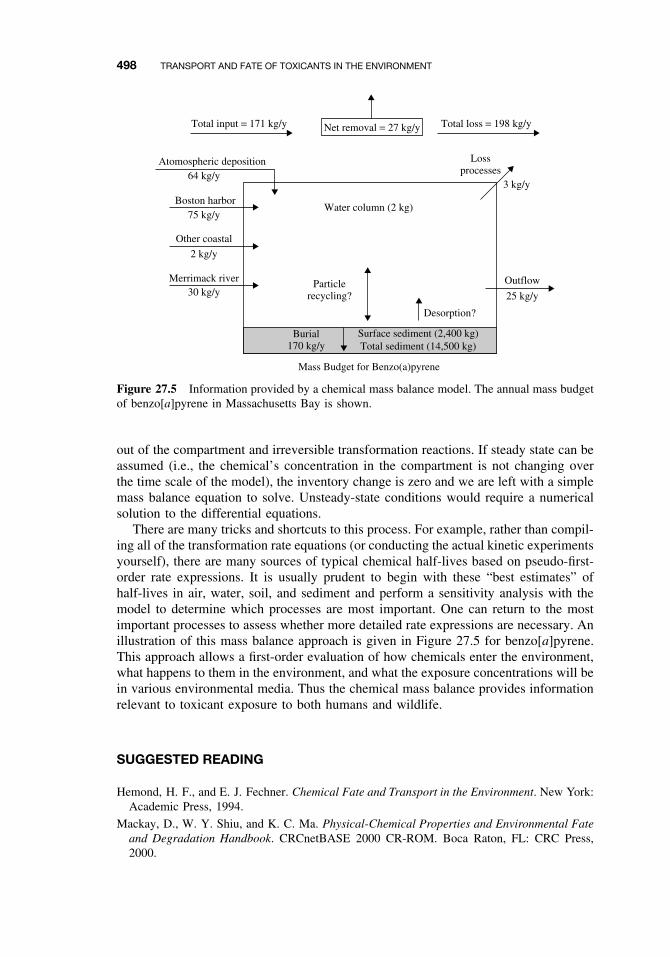
Figure 27.5 Information provided by a chemical mass balance model. The annual mass budgetof benzo[a]pyrene in Massachusetts Bay is shown.

out of the compartment and irreversible transformation reactions. If steady state can beassumed (i.e., the chemical’s concentration in the compartment is not changing overthe time scale of the model), the inventory change is zero and we are left with a simplemass balance equation to solve. Unsteady-state conditions would require a numericalsolution to the differential equations.

There are many tricks and shortcuts to this process. For example, rather than compil-ing all of the transformation rate equations (or conducting the actual kinetic experimentsyourself), there are many sources of typical chemical half-lives based on pseudo-first-order rate expressions. It is usually prudent to begin with these “best estimates” ofhalf-lives in air, water, soil, and sediment and perform a sensitivity analysis with themodel to determine which processes are most important. One can return to the mostimportant processes to assess whether more detailed rate expressions are necessary. Anillustration of this mass balance approach is given in Figure 27.5 for benzo[a]pyrene.This approach allows a first-order evaluation of how chemicals enter the environment,what happens to them in the environment, and what the exposure concentrations will bein various environmental media. Thus the chemical mass balance provides informationrelevant to toxicant exposure to both humans and wildlife.

SUGGESTED READING

Hemond, H. F., and E. J. Fechner. Chemical Fate and Transport in the Environment. New York:Academic Press, 1994.

Mackay, D., W. Y. Shiu, and K. C. Ma. Physical-Chemical Properties and Environmental Fateand Degradation Handbook. CRCnetBASE 2000 CR-ROM. Boca Raton, FL: CRC Press,2000.

SUGGESTED READING 499

Mackay, D. Multimedia Environmental Models: The Fugacity Approach, 2nd ed. Boca Raton,FL: Lewis Publishers, 2001.

Rand, G. M., ed. Fundamentals of Aquatic Toxicology: Part II Environmental Fate. Washington,DC: Taylor and Francis, 1995.

Schnoor, J. L. Environmental Modeling: Fate and Transport of Pollutants in Water, Air, and Soil.New York: Wiley, 1996.

Schwarzenbach, R. P., P. M. Gschwend, and D. M. Imboden. Environmental Organic Chem-istry, 2nd ed. New York: Wiley, 2002.

transport and fate of toxicants in the environment lieu tham khao chuong 3(1).… · transport and...

Documents