Transport in a disordered quantumdot connected to one dimensional

leads.

Transporteigenschaften einesungeordneten Quantenpunkts

angeschlossen an eindimensionaleLeiter.

Stefan Wichmann

Munich 2013

Transport in a disorderedquantum dot connected to one

dimensional leads.

Transporteigenschaften einesungeordneten Quantenpunkts

angeschlossen an eindimensionaleLeiter.

Bachelor-Thesisat the

Ludwig–Maximilians–University

submitted by

Stefan Wichmann(Matr. Nr.: 10397423)

born on the 05.09.1990 in D-92637 Weiden

supervised by

iv

Prof. Dr. Jan von Delft

andDr. Oleg Yevtushenko

Munich, the December 20, 2013

Evaluator: Prof. Dr. Jan von Delft

Day of oral exam:

Contents

1. Introduction 1

2. The emergence of the broad energy levels 13

3. The random matrix approach 143.1. The total Hamiltonian . . . . . . . . . . . . . . . . . . . . . . . . . . 143.2. Impact of the leads on the dot . . . . . . . . . . . . . . . . . . . . . . 15

4. Description of the QPC 184.1. Deriving the S-matrix for the whole system . . . . . . . . . . . . . . 184.2. Finding the scattering matrix of the QPC . . . . . . . . . . . . . . . 20

5. Numerical study of the effective Hamiltonian 235.1. Basic equations . . . . . . . . . . . . . . . . . . . . . . . . . . . . . . 235.2. Results of the calculations . . . . . . . . . . . . . . . . . . . . . . . . 245.3. Comparing the results to a constant δ model . . . . . . . . . . . . . . 26

6. Alternative description of the QPC 306.1. Composing Sc from two scatterers . . . . . . . . . . . . . . . . . . . . 306.2. How to express W in terms of rL,R . . . . . . . . . . . . . . . . . . . 33

7. Conclusion 34

A. Derivation of equation (4.21) 35

B. Code for the random matrix Hamiltonian 37

C. Code for the constant level spacing Hamiltonian 39

Bibliography 40

Acknowledgements 41

Statutory Declaration 42

1. Introduction

As smaller and smaller electric circuits can be manufactored by so called nanofab-rication [1], physics in systems of mesoscopic lengthscale plays an important role instate of the art experiments. In the mesoscopic regime, which is between the micro-scopic and the macroscopic ones, objects are small enough, so quantum mechanicbehaviour emerges, but big enough, so that a statistical description is also possible.The dimensionless conductance g = ETh

∆of such systems should be large, g � 1, so

that the following descriptions are valid. This is equivalent to the Thouless energyETh = ~

τDbeing much bigger than the average level spacing ∆, which also means

that the time τD an electron needs to traverse the system is very small. In somesamples, the mean free path of an electron can be comparable to the system size.Such systems no longer self-average a quantity like the conductance G. It becomeshighly sample dependent, whereby G loses its meaning. At temperatures below theThouless energy, universal behaviour for G can be observed again. It can be quan-tized at T < TTh in quantums of GQ = 2e2

h, called the conductance quantum, with

e being the elementary charge and h being the Planck constant [2]. In Figure 1.1experimental setups for investigation of physics on the mesoscopic length scale arepresented.

Figure 1.1.: (a) One dimensional wires. (b) A single quantum dot. (c) Three quan-tum dots A, B and C. (d) A quantum dot in an Aharonov-Bohm ring.The pictures have been copied from [3].

The brighter parts in Figure 1.1 are the gate leads, which are on top of an insulatinglayer and can be charged. Below the insulator there is the conduction material, which

2 1. Introduction

is thin enough to confine electron movement in one direction. If the conductance ofthis material is high, as stated before, the electrons inside can be described by a twodimensional electron gas. The electric field of the charged gate leads enter into thematerial below and the electron gas feels the electric field as a repulsive potential.This potential confines the electrons to certain areas, which define the shape of thesystem [2]. This mechanism is sketched in Figure 1.2. At this point it is clear, thatthe microscopic shape of such systems is hard to control and is often not known inexperimental setups. Fortunately, the microscopic details are not necessarily needed,as explained later.

Figure 1.2.: A schematic cross section of the experimental setups in Figure 1.1.

Elements, which are encountered frequently in such systems, are quantum dots(QD) and one dimensional leads. A QD is a cavity like structure, which spaciallyconfines electrons inside. The further description of these objects follow mainly [2]and [3]. A confinement of electrons to the size of QDs leads to discrete energy levelsε0j . Electrons can enter and leave the dot via attached leads if they are connected to

electron reservoirs. The more electrons are in the dot, the more energy is needed foranother electron to hop onto the dot, not only because the lower energy levels arefilled up and a single particle level spacing δj := ε0

j+1−ε0j has to be overcome, but also

because the electron repulsion due to Coulomb interaction has to be compensatedby the energy ∆EN , depending on the number of electrons N already in the dot.One can manipulate the number of electrons by attaching at least one lead to thedot and applying a gate voltage Vg, which shifts all the energy levels of the dot.Electrons can hop into or out of the dot, when the energies of the states ψn andψn+1, where the index denotes the number of electrons on the dot, is equal. This isequal to the energy difference ∆E(n) = 0 and can be archieved by tuning the gatevoltage. The energy difference can be determined from the Hamiltonian of the QD.Further electron-electron interactions to the charging energy will be neglected:

3

Hdot =∑j

εjnj + Ecn2 .

The first part of the Hamiltonian describes the discretete energy levels, that appeardue to the confinement of the electrons, εj are the energies of the single particlelevels and nj the respective electron number operators with the two eigenvalues 0or 1 for spinless electrons. The second part is the charging energy of a capacitor,Ec = e2

2Cis the charging energy, with C being the capacity of the dot, and n =

∑j nj

is the total electron number operator. ∆E(n) can be defined as the difference of theexpectation values of Hdot corresponding to the two states ψn and ψn+1. Assumingthat the lowest energy levels of the QD are filled, the difference reads:

∆E(n) = 〈ψn+1|Hdot|ψn+1〉 − 〈ψn|Hdot|ψn〉 =

=n+1∑j=1

εj + Ec(n+ 1)2 −n∑j=1

εj − Ecn2 = ε0n+1 − Vg + Ec(2n+ 1)

⇒ ∆E(n) = 0 if Vg(n) = ε0n+1 + Ec(2n+ 1) (1.1)

Figure 1.3.: Three CB peaks with CB valleys in between. The picture was takenfrom [4].

At these values of Vg, an electron can move into the dot and the conductance of thewhole system has a peak, which is called a Coulomb-blockade (CB) peak. Figure1.3 shows experimental data from [4] for the current through an Aharonov-Bohmring containing a QD. The structure of the Aharonov-Bohm ring will be describedlater. The data reveals the typical CB peak behaviour as described before. Theregion between two peaks is called the CB valley. It can be estimated from (1.1)as ∆Vg,n = Vg(n) − Vg(n − 1) = δn + 2Ec. For systems consisting of many atomsδj � Ec holds, so the width of CB valleys is almost constant, equal to 2Ec.

By attaching two leads to the dot and applying a voltage bias between them,

4 1. Introduction

Figure 1.4.: The two possible cotunneling processes. (a) Elastic cotunneling: anelectron from the left lead hops into a virtual state on the dot and offto the right lead in one move. The initial and final state have the sameenergy while the virtual state can have higher energy. In the end thereis one hole left in the left lead. (b) Inelastic cotunneling: an elctronfrom the left lead hops on the dot and another electron from the dothops off to the right lead in one move. In the end there are two holes,one in the left lead and one on the dot and one extra electron in thedot. The pictues were taken form [3].

electron transport can be realized through the dot. Usually only the lowest emptyenergy level contributes to electron transport. There are two transport regimesin such a system. One is called the single electron transfer, since in this regimethe electrons move one after another and every electron motion to or from the dotis energetically possible (∆E < 0). The other possible regime is the cotunnelingregime, in which electron movements occur simultaneously. This process is sketchedin Figure 1.4. It is energetically possible, but will be neglect in this thesis, since theyare second order processes. In an ideal system, electron transmission occours onlyat the gate voltage Vg(n), as described above. But in a real system the coupling ofthe leads to the dot can be non-trivial, for example, electrons coming from the leadcan be coupled to excited states inside the dot and not only to the lowest emptyenergy level.The irregular structure of the QD can also complicate the description ofelectron transport. Therefore, describing transport through the QD by transmissionamplitudes is better adapted to the problem.

A quantum mechanic tool to describe such a system is the scattering matrix S. Itrelates the scattering states of incoming and outgoing electrons, which are scatteredby a quantum dot, cf. Figure 1.5:

~ψout = S ~ψin (1.2)

It is important to notice, that in this case, the scattering matrix does not onlydepend on the properties of the dot but also on the coupling of the dot to the leads.This coupling usually consists of a contraction of the lead at the lead-dot interface,

5

see Figure 1.1. Such a contraction is called a quantum point contact (QPC) undersome conditions, which will be described later.

Figure 1.5.: Two leads connected to a quantum dot, which represents the scatter-ing area. Each lead has one transmitting channel with incoming andoutgoing states.

Here ψin1,2 and ψout1,2 in lead 1 and 2 are the wavefunctions for incoming and outgoingelectrons. Before going into more details about the scattering matrix, the natureof the leads should be specified . As stated earlier, the leads are confined by theelectric field of the gate wires placed on top of the conduction material. These fieldsshould be strong enough, so that the resulting potential for the electrons can bedescribed by an infinite potential well in every direction perpendicular to the lead(y-,z-direction) and by a potential constant in x-direction (parallel to the wire).For simplicity, we consider non-interacting leads, so electron-electron interactionswill be neglected and the electrons inside the leads form a free electron gas. Thisassumption is valid for experiment if the applied voltage is small enough so electronsmove one by one through the leads. Electrons can only travel in one dimension(the x-direction), therefore the leads can be described as ideal waveguides with awavefunction factorized into a part in x-direction and a part in y- and z-direction.The latter is the solution of the infinite potential well and therefore consists ofstanding waves with quantized energy levels En, which are also called channels.Only the channels with En < EF , where EF is the Fermi energy, can be occupied byelectrons and therefore contribute to electron transport. These channels are called”open” and their number is finite. Since the energy levels of an infinite potentialwell En are proportional to L−2, with L the transverse size of the wire, the numberof open channels can be reduce by making the leads narrower. A contraction of thewidth of the wire L(x) is called a QPC if the factorization of the total wavefunction isstill possible. This is true if the change of width is adiabatic, which means followingequations are true:

6 1. Introduction

∣∣∣∣dL(x)

dx

∣∣∣∣� 1 and L(x)

∣∣∣∣d2L(x)

dx2

∣∣∣∣� 1

A QPC enables to tune the number of open channels. Since the potential is constantthe wavefunction in x-direction is plane waves far from the QPC. For simplicity,we consider only one channel in every lead. The incoming waves can either bereflected from the dot or transmitted through the dot. So the outgoing waves consistof a reflected and a transmitted part. In Figure 1.5 the reflection amplitudes r1

and r2 are introduced, which describe the reflection from the dot back into lead 1and 2 respectively. Equivalently, the transmission amplidutes t12 and t21 describetransmission from one lead to the other, from 1 to 2 and from 2 to 1 respectively.All these amplitudes can be complex. The outgoing states read:

ψout1 = r1ψin1 + t21ψ

in2 , ψout2 = t12ψ

in1 + r2ψ

in2 .

With ~ψout = (ψout1 , ψout2 )T

and ~ψin = (ψin1 , ψin2 )

Tone can define the scattering matrix

from (1.2):

S =

(r1 t12

t21 r2

)(1.3)

The S matrix is unitary(S† = S−1) due to particle conservation [5]. As a result,|t12| = |t21| = T and |r1| = |r2| = R with R2 + T 2 = 1. If the scattering process

is time reversal, the S-matrix is also symmetric (ST = S), so ~ψin and ~ψout can beexchanged in (1.2). In a more general case, there are Nch channels in every leadand reflection and transmission processes can occour between any channels. Thiswill not affect the general structure or properties of the scattering matrix, but onlychange r1, r2 and t12, t21 to Nch×Nch matrices, where, for example, an entry

(t21

)kl

describes the transmission amplitude for a plane wave coming from channel l inthe second lead and going to the channel k in the first lead. The unitarity of thescattering matrix generaly leads to t12t

†12, t†12t12, t21t

†21 and t†21t21 having the same

eigenvalues {TP}. Furthermore the eigenvalues {RP} of r1r†1, r†1r1, r2r

†2 and r†2r2 are

the same with {TP}+ {RP} = 1.The current through the system can be described with the help of the Landauer for-mula, which uses the scattering matrix. By performing time and quantum mechanicaveraging, one can derive a formula for the current measured in experiment:

〈〈I〉t〉QM =GQ

e

ˆ ∞0

dE∑p

Tp(E) [f1(E)− f2(E)]

Here fi(E) is the Fermi distribution function and TP (E) describe the energy depen-dence of the eigenvalues.

Since the electron wavefunctions are plane waves in the leads, it is interesting tolook at interference experiments of these electrons. One setup for this kind of ex-periment provides the so called Aharonov-Bohm (AB) ring, which will be described

7

following [9]. The basic structure is demonstrated in Figure 1.6. Two wires in themiddle form a ring-like structure, which is connected to the outside via another twoleads. The connecting junctions can be described by 3×3 scattering matrices, sinceevery electron can either be reflected into the lead it comes from or transmitted intoone of the two wires. If a bias voltage is applied to the left (electron source) and rightlead (electron drain), electrons move through the ring. This bias should be smallenough, so that the bias drops completly at the two junctions and electrons canmove freely inside the ring. This way electrons can be reflected at the two junctionsmultiple times before leaving the ring. The electrons aquire a phase depending onthe path covered from source to drain and any applied scalar or vector potential tothe ring. The electron waves interfere in the drain lead, which results in the trans-mission amplitude for the whole system. The aquired phase of the electrons hastwo contributions, namely the dynamical phase χt and the magnetic phase φt. χtdepends on the total distance an electron covers inside the ring but not the directionin which the path is run through. It is therefore sample dependent. Furthermore,the dynamical phase depends on the electron energy and any scalar potential in thering. Denoting the phase aquired in the upper arc of the ring by χ1 and in the lowerarc by χ2, the dynamical phase reads: χt = n1χ1 + n2χ2, with ni the number ofpasses through the i-th wire.

Figure 1.6.: The structure of an AB ring connected to an electron source and drain.The Φ in the middle of the ring denotes a magnetic flux arising from anapplied magnetic vector potential. The picture was taken from [9]

φt does depend on the direction in which a path is run through. This results indifferent signs for the phase of counter clockwise and clockwise propagating electronsin the ring. the absolute value of φt depends on the magnetic flux through the ringthus, it depends on the vector potential of the magnetic field and not the magneticfield itself. The gauge degree of freedom of the magnetic vector potential translatesto φt( ~A), which is therefore also not gauge invariant. Since the total transmissionof the system must be gauge invariant, one has to find a gauge invariant quantity

8 1. Introduction

depending on the magnetic phase. This quantity is the phase aquired by a closedloop with winding number one and can be calculated as φl = πΦ

Φ0, with Φ the magnetic

flux through the ring and Φ0 = hc2e

the flux quantum. Since φt only depends on theloop number nl and the flux through the ring, it is sample independent. Denotingthe magnetic phase in the upper arc of the ring by φ1 and in the lower arc by φ2,one can find:

φt = nlφl +

{−φ1, if the particle passes lead 1 first+φ2, if the particle passes lead 2 first

Here nl is the number of clockwise loops minus the number of counter-clockwiseloops and we define: φl = φ1 + φ2. The total phase θk aquired for a certain pathlabeled by k is the sum of χt,k and φt,k. For real valued scattering matrices thetransmission through the ring reads:

T =

∣∣∣∣∣∑k

Akeiθk

∣∣∣∣∣2

=∑k,n

AkAnei(θk−θn) =

∑k,n

AkAnei(χt,k−χt,n+φt,k−φt,n) =

= Tcl + Tqm

with Tcl =∑k

A2k and Tqm =

∑k 6=n

AkAn cos (χt,k − χt,n + φt,k − φt,n) . (1.4)

Tcl and Tqm are the classical and quantum contribution to the transmission, respec-tively. Ak are weights taking into account the probability of a path k and can becalculated from the two scattering matrices representing the left and right junction.Tqm is gauge invariant, since the gauge dependent parts φ1 and φ2 of φt,k − φt,neither cancel each other or add up to a full loop in clockwise or anti-clockwise di-rection. Tqm can be further split into two contributions, a part dependent and apart independent of the dynamical phases χt,k. The former part with χt,k 6= χt,nvanishes when taking the ensemble average over χt,k. In experiment this can berealised by performing conductance measurements for either different ring setups,thus changing the length of the two arcs forming the ring, or for different chemi-cal potentials in the ring leads, and therefore using the energy dependence of thedynamical phase to change it. The second part of Tqm with χt,k = χt,n will not van-ish in an ensemble average, since the magnetic phase is independent of the sample.The arguments of the cosine functions contributing to this part have the structureφt,k − φt,n = 2mφl = 2mπΦ

Φ0, with integer m. Therefore, contributions to Tqm, which

do not depend on the dynamical phases, are periodically maximal at the same fluxΦ = sΦ0, with s a number. Any perodical dependency of a physical quantitiy on Φ

Φ0,

like the transmission amplitude in an AB ring, is called the Aharonov-Bohm effect.

In state of the art expermients, AB rings and QDs are combined. For example, theQD can be put into one arm of the AB ring, see the last panel of Figure 1.1. It wasshown in [4], that coherent electron transport through a quantum dot is possible if

9

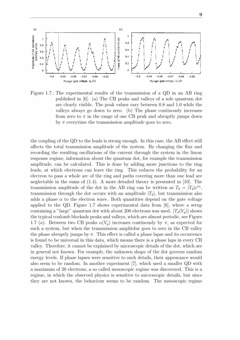
Figure 1.7.: The experimental results of the transmission of a QD in an AB ringpublished in [6]. (a) The CB peaks and valleys of a sole quantum dotare clearly visible. The peak values vary between 0.8 and 1.0 while thevalleys always go down to zero. (b) The phase continously increasesfrom zero to π in the range of one CB peak and abruptly jumps downby π everytime the transmission amplitude goes to zero.

the coupling of the QD to the leads is strong enough. In this case, the AB effect stillaffects the total transmission amplitude of the system. By changing the flux andrecording the resulting oscillations of the current through the system in the linearresponse regime, information about the quantum dot, for example the transmissionamplitude, can be calculated. This is done by adding more junctions to the ringleads, at which electrons can leave the ring. This reduces the probability for anelectron to pass a whole arc of the ring and paths covering more than one lead areneglectable in the sums of (1.4). A more detailed theory is presented in [10]. Thetransmission amplitude of the dot in the AB ring can be written as Td = |Td|eiα,transmission through the dot occurs with an amplitude |Td|, but transmission alsoadds a phase α to the electron wave. Both quantities depend on the gate voltageapplied to the QD. Figure 1.7 shows experimental data from [6], where a setupcontaining a ”large” quantum dot with about 200 electrons was used. |Td(Vg)| showsthe typical coulomb blockade peaks and valleys, which are almost periodic, see Figure1.7 (a). Between two CB peaks α(Vg) increases continously by π, as expected forsuch a system, but when the transmission amplitdue goes to zero in the CB valleythe phase abruptly jumps by π. This effect is called a phase lapse and its occurrenceis found to be universal in this data, which means there is a phase laps in every CBvalley. Therefore, it cannot be explained by microscopic details of the dot, which arein general not known. For example, the unknown shape of the dot governs randomenergy levels. If phase lapses were sensitive to such details, their appearance wouldalso seem to be random. In another experiment [7], which used a smaller QD witha maximum of 20 electrons, a so called mesoscopic regime was discovered. This is aregime, in which the observed physics is sensitive to microscopic details, but sincethey are not known, the behaviour seems to be random. The mesoscopic regime

10 1. Introduction

emerges if 10 or less electrons are in the dot [7]. The more electrons are in a QD thesmaller is its levelspacing and the higher becomes the charging energy of the dot. Toinvestigate whether these quantities trigger the change from the mesoscopic to theuniversal regime, a numerical approach, focusing on the interplay between the levelspacing δj of the energy levels of the dot, their widths Γj and the charging energyU , was done in [8].The model used in this numerical simulation consists of three parts. Firstly spinlesselectrons in the QD are described by the Hamiltonian:

Hdot =N∑j=1

εjnj +1

2U∑j 6=j′

(nj −

1

2

)(nj′ −

1

2

)(1.5)

whwew N is the number of levels contributing to the transmission, εj is the energy

and nj = d†j dj the particle number operator of the j-th state. d†j/dj are the cre-ation/annihilation operators for spinless electrons of the j-th state in the dot. U > 0describes the Coulomb interaction inside the dot and is therefore a charging energywhich seperates the CB peaks. The energy levels of the dot can be shifted by thegate voltage and define the single particle level spacing δj = εj+1− εj and the meanlevel spacing ∆ = 1

N

∑j δj.

The second part of the model is the Hamiltonian for the leads:

Hl = −t∞∑m=0

(c†m,lcm+1,l + h.c.

)(1.6)

which describes a semi-infinite tight-binding chain with a zero on-site energy. t isthe hopping amplitdue and c†m,l/cm,l the creation/annihilation operators for the m-th site of the lead l. Two leads, left and right, were used in this paper, so l = L,R.The site with m = 0 is the one closest to the QD, see Figure 1.8. The Hamiltoniandescribes a system, in which only one electron per site is allowed, so electrons moveone by one. Furthermore the electrons can only hop to their nearest neighbours.The last part of the model describes the lead-dot coupling:

HT = −∑j,l

(tlj c†0,ldj + h.c

). (1.7)

Here tlj are the coupling amplitudes for the j-th channel inside the dot and thel-th lead connected to the dot. The site m = 0 of the lead is coupled to the QD,see Figure 1.8. The coupling amplitudes define the level width via Γj =

∑l πν|tlj|2

where ν is the local energy-independent density of states of the lead, calculated onthe site m = 0.By assuming a constant level spacing δ, it was observed, that if δ ≤ Γ and |Γ−δ| � δ,as many energy levels as leads attached to the QD become much wider than theothers. Furthermore the position of these broad levels as a function of gate voltageis almost constant over a large interval of Vg if U 6= 0. In this interval, the energy ofthe broad levels is close to the chemical potential of the leads. After changing the

11

Figure 1.8.: Sketch of the tight binding model for the left lead.

gate voltage in this interval, the remaining narrow energy levels cross the wide ones.This overlap enables electron transport in two or more energy levels simultaniously,which leads to interference effects. The transmission zero accopanying every phaselapse indicates destructive interference between transmitting channels. Interferencesin a setup of a discrete energy level overlapping with a continuum of possible energies,can be described by Fano-type antiresonances, which are accompanied by a phaselapse [13]. The discrete energy level can be identified with a narrow energy leveland the continuum with a broad energy level [8]. To summarize, the importantconditions for the occurence of a phase lapse are δ ≤ Γ, |Γ − δ| � δ and U 6= 0.It was noticed that the the broad energy levels exist for U = 0 aswell. Some ofthe results of numericial calulations in the universal regime can be seen in Figure1.9. The red line is the position of the broad energy level. It is almost constantfor a wide range of gate voltage. Everytime one of the three narrow energy levelscrosses the red line a phase laps and transmission zero occurs. For U ≥ Γ the CBpeaks are well seperated and the typical behaviour of phase can be observed. Byfurther increasing the charging energy to U � Γ, the resulting curve matches theexperimental results.

12 1. Introduction

Figure 1.9.: The top panel shows the energy levels of the dot changing with gatevoltage. The Fermi level of the lead was set to zero. The red line is theposition of the broad energy level which is almost zero for a wide rangeof Vg. The phase and the absolute vlaue of the transmission amplitudeare plotted in the lower panel. The data was taken from [8].

2. The emergence of the broadenergy levels

The presented explanation for the phase lapses taken from [8] depends cruciallyon the existence of the broad energy levels. The Hamiltonian for the dot and aconstant level spacing was assumed for the simulations. It was proposed, that asmall deviation from the latter assumption does not change the results. However theassumption about a regular nature of the QD spectrum and even more importantly,about the specific lead-dot coupling considered in [8] can substantially disagree withexperiments. In particular, the energy levels inside the dot are not known and veryrandom. Also the coupling of the QD to the leads can be very different. For examplea lead can be connected to many levels inside the dot or only to a few. But sincethe phase lapses occur in different QDs, the explanation of this effect must notdepend the assumption of constant level spacing or a specific coupling. Thereforeit is left to study, whether the occurence of the broad energy levels depends onthe above mentioned assumptions or if it is a more general effect arising from thegeneric coupling to the leads. A more general model, which can be derived frommicroscopic assumptions and takes the randomness of the QD into account will bestudied in this thesis. The focus will be on the occurance and stability of the broadenergy levels and on finding the relevant regimes where it appears. This is doneby numerically diagonalizing the Hamiltonian of the system. The distribution ofthe energy widths will be investigated and its dependencies on the number of levelsinside the dot and the strength of the coupling between the dot and the lead willbe studied. Furthermore a generalization of the description for the QPC will besuggested.

3. The random matrix approach

3.1. The total Hamiltonian

The model, that is used in this thesis, consists of three parts which describe spinless,non-interacting electrons. Furthermore, we put ~ = 1 for the whole thesis. The firstpart is HD, describing the QD, the second is HL, describing the leads and the lastis HLD, describing the coupling of the leads to the QD and therefore resembles theQPC. Since properties of electron transport, which mostly origins from electronswith energies close to the Fermi energy, are of interest, the electrons in the leads canbe discribed by the linearized, one dimensional dispersion relation of a free electrongas. By assuming non-interacting leads, HL reads:

HL = vF

Nch∑j=1

ˆdk

2πkψ†j(k)ψj(k) . (3.1)

Here Nch is the number of open channels in the lead, vF is the Fermi velocity andk is the wavevector relative to the Fermi level; ψ†j(k)/ψj(k) are the fermionic cre-ation/annihilation operators for electrons in channel j in momentum representation.If more than one lead is attached to the QD, Nch is the sum of the open channelsin every lead. Assuming a random potential U inside the QD, HD reads:

HD =

ˆd~r

[1

2m~∇a†~∇a+ Ua†a

]with electron creation/annihilation operators a†/a and electron mass m. It is known[2] that such a Hamiltonian can be split into two parts: a universal part H(0), whichis corresonds to g → ∞, and a non-universal part H(1/g), which is proportional tog−1. Since g >> 1, H(1/g) is small and will be neglected. Since interactions [11] areneglected in this thesis, the Hamiltonian for the QD reads:

HD =M∑

α,γ=1

Hαγφ†αφγ . (3.2)

M is the number of energy levels in the QD and φ†α/φα are the respective creationannihilation operators. Hαγ are the entries of a random hermitian M ×M matrix(H = H†) from the WD Gaussian ensemble. Its elements are Gaussian distributedwith the correlation function

3.2 Impact of the leads on the dot 15

〈HαγHα′γ′〉 =M∆2

π2

[δαγ′δα′γ +

(2

β− 1

)δαα′δγγ′

]. (3.3)

Here β is the Dyson symmetry parameter, which reflects time-reversal symmetry.For β = 1 the system has time-reversal symmetry resulting in H real and for β =2 the system has no time-reversal symmetry resulting in H complex with equalvariances of imaginary and real parts of Hij. For simplicity, time-reversal symmetryis assumed (β = 1) in this thesis. ∆ = πM−1/2 is the mean, one electron levelspacing for a Gaussian orthogonal distribution in the dot [14], so (3.3) reduces to:

〈HαγHα′γ′〉 = δαγ′δα′γ + δαα′δγγ′ . (3.4)

The last part of the model is the coupling of the lead to the dot:

HLD =

Nch∑j=1

M∑α=1

ˆdk

2π

[Wαjφ

†αψj(k) +Wαjψ

†j(k)φα

]. (3.5)

Here Wαj are the elements of a real M × Nch matrix (W = W ∗) describing thecoupling of the dot and the lead, so this parameter represents the QPC. The totalHamiltonian is the sum of the three parts:

Htot = HD + HL + HLD . (3.6)

3.2. Impact of the leads on the dot

Since we focus on the properties of the QD, the leads will be integrated out in Htot

to find an effective Hamiltonian Heff describing only the QD and the QPC. We canwrite the total Hamiltonian as:

Htot = HL ⊗ 1D + 1L ⊗ HD + HLD .

The wavefunction it acts on has the structure: |ψL〉⊗ |ψD〉, with a wavefunction forthe lead |ψL〉 and the dot |ψD〉. To find Heff , a quantum mechanic averaging with

the groundstate wavefunction of the lead is performed: Heff = 〈Htot〉L . 〈HL〉L1D is

a number and can therefore be neglected. 〈1L〉LHD = HD since the wavefunctionsare normalized. The expectation value of the Hamiltonian for the coupling of thelead and the dot 〈HLD〉L yields the self energy Σ in a Green’s function approach.The Dyson’s equation for a Green’s function for the dot reads:

G−1D (ε = 0) =

(G0D(ε = 0)

)−1

− Σ (3.7)

Where G0D(ε = 0) =

(HD

)−1

and GD(ε = 0) =(Heff

)−1

. Σ describes a hop-

ping of electrons to and from the QD. The only non vanishing contribution to Σ is

16 3. The random matrix approach

〈HLDHLD〉L. It describes an electron hopping to the lead and back to the dot againwithout any propagation in the lead, so it depends on the Green’s function in thelead at x = 0: G0

L(0, 0;ω). For easier calculations, the basis of ψ†j(k)/ψj(k) in HLD

will be changed from momentum to real space represantation.

ψj(k) =

ˆdx〈k|x〉ψj(x) =

ˆdx e−ikxψj(x) (3.8)

ψ†j(k) =

ˆdx〈x|k〉ψ†j(x) =

ˆdx eikxψ†j(x) (3.9)

This yields HLD in real space representation:

HLD =

Nch∑j=1

M∑α=1

[Wαjφ

†αψj(0) +Wαjψ

†j(0)φα

]. (3.10)

By using

〈ψ†i (x)ψ†j,(x)〉L = 〈ψi(x)ψj(x)〉L = 0 ∀i, j

〈ψ†i (x)ψj(x)〉L = 〈ψi(x)ψ†j(x)〉L = 0 for i 6= j

we find with omitting x = 0 dependencies:

〈HLDHLD〉L =M∑

α,β=1

Nch∑j=1

Wα,jWβ,j

[〈ψjψ†j〉Lφ†αφβ + 〈ψ†j ψj〉Lφαφ

†β

]=

=M∑

α,β=1

Nch∑j=1

Wα,jWβ,j

[〈ψjψ†j〉Lφ†αφβ + 〈ψ†j ψj〉Lφβφ†α

]=

=M∑

α,β=1

φ†α

[〈ψjψ†j〉L − 〈ψ

†j ψj〉L

]︸ ︷︷ ︸

=iG0L

[WW †]

αβφβ =

=M∑

α,β=1

φ†α

(iG0

L

[WW †]

αβ

)φβ . (3.11)

By using the Feynman rules [15], one can express the self energy as: Σαβ = −iVαβG0L.

It follows from (3.11) that Vαβ = i[WW †]

αβ. G0

L(0, 0;ω) = ∓πiν(ω) [5], ν(ω) ≈ν(εF ) = ν is the density of states in the lead at the Fermi energy, since ω ≈ εF . Thesign of G0

L must correspond to the retardation (− retarded, + advanced). In totalthe selfenergy reads:

Σαβ = ∓iπν[WW †]

αβ. (3.12)

The effective Hamiltonian with the retarded self energy reads:

3.2 Impact of the leads on the dot 17

Heff =M∑

α,β=1

(Hαβ + iπν

[WW †]

αβ

)φ†αφβ . (3.13)

The coupling of the leads to the dot yields an imaginary contribution to the eigen-values. The imaginary part of the eigenvalues of (3.13) determines the life timeofthe state, which is inverse to the level broadening. The highest possible rank ofthe matrix WW † is the number of channels in the leads Nch by construction. Sothe number of non zero eigenvalues of the selfenergy matrix is Nch and the numberbroadened energy levels is expected to be also Nch [8].

4. Description of the QPC

To find the coupling matrix W , the scattering matrix for the whole system will bederived and seperated in parts originating from the QD and the QPC.

4.1. Deriving the S-matrix for the whole system

This section follows the Appendix C of [2]. As stated in the introduction, the S-matrix relates incoming and outgoing electrons. Equation (1.2) for each channeltakes the form:

aouti =

Nch∑j=1

Sijainj (4.1)

with aouti /ainj the amplitudes of the outgoing/incoming electrons in channel i/j. Weassume that the 1-D interference is at x = 0, see Figure [?].

Figure 4.1.: Definition of the coordinates at a lead-dot interface. The picture wastaken from [2].

As explained in the introduction, the wavefunction for all electrons in the leadconsists of plane wave contributions with an amplitude Φj(~r⊥) depending on theperpendicular coordinates. With k = ε

vF, the wavefunction reads:

4.1 Deriving the S-matrix for the whole system 19

ψe(~r) =

Nch∑j=1

Φj(~r⊥)

[ainj e

i(kF + ε

vF

)x

+ aoutj e−i

(kF + ε

vF

)x

](4.2)

The corresponding annihilation operator can be written as:

ψe(~r) =

Nch∑j,l=1

Φj(~r⊥)

ˆdk

2π

[U∗jle

i(kF +k)x + Ujle−i(kF +k)x

]ψj(k) (4.3)

where U describes the boundary conditions at x = 0. If there is no coupling to thedot, electrons will be reflected at x = 0, resulting in a phaseshift of π without mix-ing channels. This way all channels are incorporated into one matrix. The Dirichletboundary condition, ψe(0) = 0 yields Ujl = iδjl, if the boundary is an infinite wall.

For easier calculations, the basis of ψ†j(k)/ψj(k) in HL will be changed from momen-tum to real space represantation, see equations (3.8) and (3.9). The result reads:

HL = −ivFNch∑j=1

ˆdx ψ†j(x)

d

dxψj(x) . (4.4)

Denoting the single electron wavefunctions for each channel in the lead by ψj and inthe dot by φα and the ground state by ψ0 in the leads and φ0 in the dot respectivly,the creation/annihilation operators act as follows:

ψj(x′)ψi(x) = δijδ(x− x′)ψ0 (4.5)

ψ†j(x)ψ0 = ψj(x) (4.6)

φαφγ = δαγφ0 (4.7)

φ†αφ0 = φα (4.8)

Writing down the Schrodinger equation with the total Hamiltonian (3.6) for theleads, with the wavefuntion ψi(x)⊗φ0, and for the dot, with the wavefuntion ψ0⊗φα,yields the equations:

εψi(x) = ivFdψi(x)

dx+

M∑α=1

W ∗αiδ(x)φα (4.9)

εφβ =M∑α=1

Hβαφα +

Nch∑j=1

Wβjψj(0) (4.10)

At x < 0, equation (4.9) describes a left moving particle. Using (4.2), (4.9) and(4.10), we can find ψj(x):

20 4. Description of the QPC

ψj(x) =

e−ikx∑Nch

l=1 Ujlainl , x = +0

12

∑Nch

l=1

(Ujla

inl + U∗jla

outl

), x = 0

e−ikx∑Nch

l=1 U∗jla

outl , x < 0

(4.11)

with the proper normalization at x = 0. The unknown wavefunction inside the QDcan now be eliminated with (4.9) and (4.10). But before the divergence in (4.9) atx = 0 has to be taken care of. Let us integrate over x from −ε to ε in the limitε→ 0:

ε limε→0

ˆ ε

−εψj(x)dx︸ ︷︷ ︸

→0, since ψj(0) finite

= limε→0

ˆ ε

−εivF

∂ψj(x)

∂xdx+ lim

ε→0

ˆ ε

−ε

M∑ν=1

W ∗νjδ(x)φνdx

⇒ 0 = limε→0

ivF (ψj(+ε)− ψj(−ε)) +M∑ν=1

W ∗νjφν (4.12)

Reading a(in/out)l and φα as vector entries and substituting (4.11) into (4.10) and

(4.12), yields:

ivF(U~a(in) − U∗~a(out)

)+W †~φ = 0 (4.13)

ε~φ = H~φ+1

2W(U~a(in) + U∗~a(out)

)(4.14)

Now we can eliminate the wavefunction inside the dot ~φ in (4.13)-(4.14) and find~a(out), cf. (4.1). This yields the scattering matrix:

S(ε) = UT[1− iπνW † (H − ε)−1W

]−1 [1 + iπνW † (H + ε)−1W

]U (4.15)

Here the density of states in the one dimensional leads ν = 12πvF

has been introduced.

4.2. Finding the scattering matrix of the QPC

Since we want to investigate the coupling of the QD to the leads, it is convenientto seperate the S matrix of the total system into parts coming from the QPC andthe QD. The following calculation is taken from [12]. If two leads with N channelseach are connected to a scattering region, QPC a 2N × 2N scattering matrix withtime-reversal symmetry is assumed, so it has the structure:

Sc =

(rc tTctc r′c

)

4.2 Finding the scattering matrix of the QPC 21

where rc/tc describes the reflection/transmission to the dot for waves coming fromthe leads and r′c/t

Tc the reflection/transmission to the leads for waves coming from

the dot. Let’s denote the scattering matrix of the QD by S0. The total scatteringmatrix must account for all pathes, on which an incoming electron can leave thedot:

S(ε) = rc + tTc S0(ε)tc + tTc S0(ε)r′cS0(ε)tc + tTc S0(ε)r′cS0(ε)r′cS0(ε)tc + ...

The first term is direct reflection at the QPC and the remaining terms describemultiple reflections between the QPC and the QD before leaving the dot. This is ageometric series and thus S(ε) can be written in the form:

S(ε) = rc + tTc S0(ε) [1− r′cS0(ε)]−1tc (4.16)

To split S(ε) this way we first use a parametrization of W from [2]:

W = NV OW . (4.17)

Here N is a normalization constant, V is an orthogonal M×M matrix, O is a M×Nprojection matrix with Omn = δmn and W is a real N ×N matrix, which describesthe QPC. The normalization in [2] corresponds to a Lorentzian distribtution [12],so it must be adapted to fit the Gaussian distribution, which we use. It can befound by calculating the scattering matrix for H = 1 and assuming a ballistic QPC,which means that the reflection amplidtudes are zero. In this case, electrons withzero energy can only aquire a phase in the scattering process. Thus the scatteringmatrix must be the identity matrix multiplied with a phase factor eiΘ:

eiΘ = −[1− iπνW †W

]−1 [1 + iπνW †W

]⇔ W †W = − 1

πν

sin Θ

(1− cos Θ)

Choosing Θ = 32π to get an easy expression, yields for the nomalization factor

N = 1√πν

. Thus, (4.17) reduces to:

W =1√πνV OW . (4.18)

Inserting (4.18) into (4.15) yields:

S(ε) = U[1 + iW †H(ε)W

] [1− iW †H(ε)W

]−1

UT (4.19)

where H = O†V † (H − ε)−1 V O was introduced. Since the distribution P (H) isinvariant under the orthogonal transformation, the rotation caused by V and V T ,does not change the distribution of the entries of H, one can argue that H stilldescribes only the random QD with the Hamiltonian taken from the WD-RMT. If

22 4. Description of the QPC

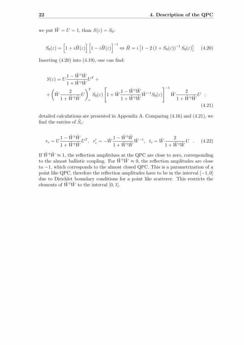
we put W = U = 1, than S(ε) = S0:

S0(ε) =[1 + iH(ε)

] [1− iH(ε)

]−1

⇔ H = i[1− 2 (1 + S0(ε))−1 S0(ε)

](4.20)

Inserting (4.20) into (4.19), one can find:

S(ε) = U1− W †W

1 + W †WUT +

+

(W

2

1 + W †WU

)Tc

S0(ε)

[1 + W

1− W †W

1 + W †WW−1S0(ε)

]−1

W2

1 + W †WU ;

(4.21)

detailed calculations are presented in Appendix A. Comparing (4.16) and (4.21), wefind the entries of Sc:

rc = U1− W †W

1 + W †WUT , r′c = −W 1− W †W

1 + W †WW−1, tc = W

2

1 + W †WU . (4.22)

If W †W ≈ 1, the reflection amplitdues at the QPC are close to zero, correspondingto the almost ballistic coupling. For W †W ≈ 0, the reflection amplitudes are closeto −1, which corresponds to the almost closed QPC. This is a parametrization of apoint like QPC, therefore the reflection amplitudes have to be in the interval [−1, 0]due to Dirichlet boundary conditions for a point like scatterer. This restricts theelements of W †W to the interval [0, 1].

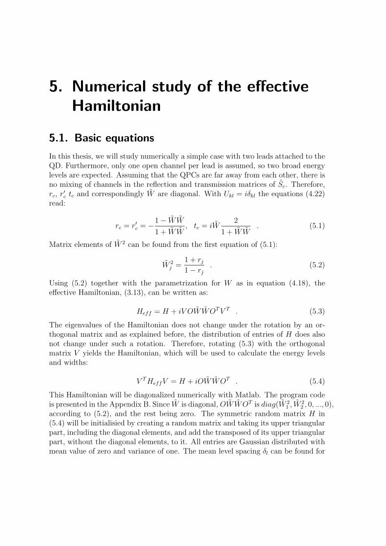
5. Numerical study of the effectiveHamiltonian

5.1. Basic equations

In this thesis, we will study numerically a simple case with two leads attached to theQD. Furthermore, only one open channel per lead is assumed, so two broad energylevels are expected. Assuming that the QPCs are far away from each other, there isno mixing of channels in the reflection and transmission matrices of Sc. Therefore,rc, r

′c tc and correspondingly W are diagonal. With Ukl = iδkl the equations (4.22)

read:

rc = r′c = −1− WW

1 + WW, tc = iW

2

1 + WW. (5.1)

Matrix elements of W 2 can be found from the first equation of (5.1):

W 2j =

1 + rj1− rj

. (5.2)

Using (5.2) together with the parametrization for W as in equation (4.18), theeffective Hamiltonian, (3.13), can be written as:

Heff = H + iV OWWOTV T . (5.3)

The eigenvalues of the Hamiltonian does not change under the rotation by an or-thogonal matrix and as explained before, the distribution of entries of H does alsonot change under such a rotation. Therefore, rotating (5.3) with the orthogonalmatrix V yields the Hamiltonian, which will be used to calculate the energy levelsand widths:

V THeffV = H + iOWWOT . (5.4)

This Hamiltonian will be diagonalized numerically with Matlab. The program codeis presented in the Appendix B. Since W is diagonal, OWWOT is diag(W 2

1 , W22 , 0, ..., 0),

according to (5.2), and the rest being zero. The symmetric random matrix H in(5.4) will be initialisied by creating a random matrix and taking its upper triangularpart, including the diagonal elements, and add the transposed of its upper triangularpart, without the diagonal elements, to it. All entries are Gaussian distributed withmean value of zero and variance of one. The mean level spacing δl can be found for

24 5. Numerical study of the effective Hamiltonian

every realization l of H from the real parts of the eigenvalues λ:

∆l =max [Re (λ)]−min [Re (λ)]

M. (5.5)

The mean level widths Γl of every realization is calculated just as ∆l, but with theimaginary parts of the eigenvalues. Averaging both quantities over many realizationsof H gives the total mean level spacing ∆ and the total mean level width Γ. ∆ willbe compared to Γ and is used as an unit for the level widths γi. Using the levelwidths for many realizations of the random matrix H, enables us to plot statistics.

5.2. Results of the calculations

Figure 5.1.: Histogram for an almost closed QPC. (a) The distribution of all valuesof γi. (b) Zoomed in at higher values of γ.

First, the γi of L = 105 realizations are plotted in a histogram H(γ), which isnormalized so

´H(γ)dγ = 1. For an almost closed QPC, where r1 and r2 are close

to −1, the result is shown in Figure 5.1. The distribution 5.1(a) can be fitted quitewell by an exponential decay, with the most probable level width at zero. Sincewe are interested in the broad energy levels, the same distribution zoomed in athigher values of γ is shown in Figure 5.1(b). At higher values, the distribution stilllooks like an exponential decay and there is no behaviour indicating the existanceof stable broad energy levels. Due to the long tail of the distribution, fluctuations ofthe broad energy levels are large. Since Γ

∆≈ 0.008� 1, this behaviour is expected

5.2 Results of the calculations 25

[8].The same plots for an almost ballistic QPC,where r1 and r2 are close to 0, areshown in Figure 5.1. The behaviour is qualitativly the same as for the almost closedQPC. The distribution looks like an exponential decay, but is flatter than in thealmost closed QPC, so there is a trend to broader energy levels. But there is still nopeak at higher level widths, which would indicate a scale seperation. Γ

∆≈ 0.051 is

still much smaller than one. The trend is a higher ratio Γ∆

for reflection amplitudescloser to zero. For rj = 0, Γ

∆≈ 0.075 is the maximal value, which can be reached

in this model. This is still far from the regime Γ∆≥ 1, which was observed for the

existance of the broad energy levels in [8].

Figure 5.2.: Histogram for an almost ballistic QPC. (a) The distribution of all valuesof γi. (b) Zoomed in at higher values of γ.

Since there can still be a scale seperation in this model, which is just not visible inthe statistics of many realizations of disorder in the QD due to strong fluctuations,γi of several, randomly choosen, realizations are plotted in Figure 5.3 and 5.4. Inpanel (a) of each Figure, a single realization of γi is plotted. After looking at manyrandomly picked realizations, both were chosen to reflect the typical pictures. Forthe almost closed as well as for the almost ballistic QPC, there is no scale seperationat all. In rare cases, there are gaps in between the level widths, but that is due to thefluctuations arising from the random matrix and do not reflect a stable distributionof energy widths. In panel (b) of 5.3 and 5.4, 10 realizations of γi are plotted.The fluctuations of the two highest energy levels overlap with the fluctuations of thenarrow energy levels, so no gap in the level widths can be seen. The other parameterwhich can be changed in this model is M , the number of energy levels inside the

26 5. Numerical study of the effective Hamiltonian

Figure 5.3.: Randomly choosen realizations of disorder for the almost closed QPC.(a) γi of a single realization, which was found to be typical in thisconfiguration. (b) γi of 5 different realizations.

QD. As M decreases, it scales the total mean level width Γ, but does not changethe qualitative behaviour of the system, down to M = 5. At this point Γ

∆≈ 0.25

and there is still no gap seperating broad and narrow energy levels. Increasing Mreduces the ratio Γ

∆even further and does not bear new results.

In this model the regime of the broad energy levels could not be reached, sinceΓ∆� 1. So far rj are bounded to rj ∈ [−1, 0], which reflects a coupling of W 2

j ∈ [0, 1](cf. Eq.(5.2)). Relaxing this constriction to rj ∈ [−1, 1] reflects an arbitrary couplingwith no bounds. The only possibility to enter the regime ∆

Γ≥ 1 is using stronger

couplings W 2 and therefore violating the constrictions of the point like scatterer.Using rj > 0 to see whether broad energy levels exist for stronger couplings yieldsthe results in Figure 5.5. Additionally peaks can be observed in the statistics as theregime Γ

∆≈ 1 is entered, so broad energy levels mathematically exist in the RMT

model and an alternative description of the QPC could help.

5.3. Comparing the results to a constant δ model

In this section we reproduce numerical results obtained in [8] for the model describedin the introduction and compare them with our findings for the RMT-based model.The structure of the effective Hamiltonian in [8] is:

5.3 Comparing the results to a constant δ model 27

Figure 5.4.: Randomly choosen realizations of disorder for the almost ballistic QPC.(a) γi of a single realization, which was found to be typical in thisconfiguration. (b) γi of 5 different realizations.

Heff,c = h+ iπνttT . (5.6)

t is the M × Nch coupling matrix from (1.7) and h is a M ×M diagonal matrixwith the entries εi from (1.5). The levelspacing is constant and equal the mean levelspacing from the random matrix model, so the results are comparable: ∆ = 0.5322for M = 50. The coupling matrix t will be parametrized as W before:

t =1√πνV Ot . (5.7)

Here t is a diagonal Nch ×Nch matrix and V is used to get a full coupling matrix.

→ Heff,c = h+ iV OttTOTV T . (5.8)

The mean level width Γ is given by:

Γ =πν

M

∑αj

t2αj =πν

MTr[ttT]

=1

MTr[OttOT

](5.9)

Assuming two leads with one channel in each lead, t can be parametrized by areflection amplitude rj, Eq. (5.2) after substitutiong t for W . This way the coupling

28 5. Numerical study of the effective Hamiltonian

Figure 5.5.: Histogram for an almost ballistic QPC with positice reflection ampli-tudes. (a) All values. (b) Zoomed in at higher γ.

strengths can be compared to the previous calculations. Since t has no restrictionsin [8], it will be taken from the interval [−1, 1]. V is chosen as the symmetriceigenvector matrix for second difference matrix (taken from the help catalogue ofMatlab) to get an easy way of getting an orthogonal matrix of any size. The programcode can be found in appendix C. The results are summarized in Figure 5.6. Firstly,we study negative r1,2 similar to the RMT model for the almost ballistic QPC, seepanel (a). In this case Γ

∆<< 1 there is no gap between broad and narrow energy

levels. For positive reflection amplitudes rj, a seperation of scales can be observedat at Γ

∆≈ 0.25, see Figure 5.6(b)-(d). This is in a qualitative agreement with [8]. So

neither in the diagonal model nor in the RMT model do broad energy levels existfor rj ∈ [−1, 0], while both models show a gap for rjin[0, 1].

5.3 Comparing the results to a constant δ model 29

Figure 5.6.: Level widths of a diagonal Hamiltonian for the dot with constant levelspacing. (a) Negative reflection amplitdues as in the previous model.There is no gap between broad and narrow energy levels. (b)-(d) A gapemerges and becomes clearly visible at positive rj, where Γ→ ∆.

6. Alternative description of theQPC

In the previous chapter it was shown that broad energy levels do not exist withinthe restriction of rj ∈ [−1, 0]. This restriction origins at the Dirichlet boundaryconditions for the point like QPC. Therefore a different description of the QPC,with different boundary conditions, is needed. A possible solution is a QPC with afinite width of boundaries, which must be described by their own S-matrices withoutrestrictions assumed for point like scatterers.

6.1. Composing Sc from two scatterers

To parametrize the QPC, a left and a right boundary of the QPC is defined. Theboundaries can be represented by the two scattering matrices SL/R, which are unitaryand assumed to be time-reversal (SL/R = STL/R) and left-right symmetric (SL/R =

τ2SL/Rτ2, with τ2 being the Pauli matrix). Furthermore, no mixing of channels isassumed, so the reflection and transmission matrices in the scattering matrix arediagonal. The unitarity condition for a S-matrix with diagonal entries yields anequivalent and independent set of equations for every channel, so only a one channelproblem has to be solved. Therefore, a one channel problem will be considered fromhere on and channel indices will be omitted. From the general parametrization of a2× 2 unitary matrix

S = eiφ(

cos (α)eiν i sin (α)eiµ

i sin (α)e−iµ cos (α)e−iν

)the conditions for the imposed symmetries can be found. Time-reversal symmetrieyields: eiφi sin (α)eiµ = eiφi sin (α)e−iµ ⇔ µ = 0 and left-right symmetry yields:eiφ cos (α)eiν = eiφ cos (α)e−iν ⇔ ν = 0. Introducing rL/R = cos (αL/R) and tL/R =sin (αL/R) so r2

L/R + t2L/R = 1 results in:

SL/R = eiφL/R

(rL/R itL/RitL/R rL/R

). (6.1)

In the most general case Sc matrix has the structure as stated in (1.3), but it can stillbe multiplied by a global phase factor eiΦ without violating the unitarity condition:

Sc = eiΦ(rc t′ctc r′c

).

6.1 Composing Sc from two scatterers 31

rc/tc and r′c/t′c are matrices describing reflection/transmission from the left and the

right respectively. To compose Sc from SL/R, all paths that traverse both bound-aries of the QPC are summed up in tc/t

′c and all paths that do not traverse both

boundaries yield rc/r′c. Figure 6.1 illustrates this procedure.

Figure 6.1.: (a) Paths adding up to the reflection of the QPC. (b) Paths adding upto the transmission of the QPC.

Because of this construction, the assumption of non-mixing channels in SL/R trans-fers to Sc. The entries of Sc read:

rc = eiφLrL − ei(2φL+φR)tLrRtL − ei(3φL+2φR)tLrRrLrRtL − ...

→ rc = eiφLrL −ei(2φL+φR)t2LrR

1− ei(φL+φR)rRrL= eiφL

rL − ei(φL+φR)rR1− ei(φL+φR)rRrL

(6.2)

tc = −ei(φL+φR)tLtR − ei(2φL+2φR)tLrRrLtR − ...

→ tc = − ei(φL+φR)tLtR1− ei(φL+φR)rRrL

(6.3)

r′c and t′c follow by exchanging L and R in the indices. It follows that tc = t′c, so thetime-reversal symmetry also transfers from SL/R to Sc. r

′c reads:

r′c = eiφRrR − ei(φL+φR)rL1− ei(φL+φR)rRrL

(6.4)

So whether the entries of Sc are real or complex depends on the global phases φLand φR. In this case the unitarity condition ScS

†c = 1, yields:

eiΦ(rc tctc r′c

)e−iΦ

(r∗c t∗ct∗c r′∗c

)=

(rcr∗c + tct

∗c rct

∗c + tcr

′∗c

tcr∗c + r′ct

∗c tct

∗c + r′cr

′∗c

)=

(1 00 1

).

32 6. Alternative description of the QPC

This is equivalent to the three independent equations:

|rc|2 + |tc|2 = 1 (6.5)

tcr∗c + r′ct

∗c = 0 (6.6)

|r′c|2 + |tc|2 = 1 (6.7)

With rc, r′c and tc it can be validated if the constructed Sc can be unitary:

|rc|2 = |r′c|2 =r2L + r2

R − 2 cos (φL + φR)rLrR1 + r2

Lr2R − 2 cos (φL + φR)rLrR

|tc|2 =t2Lt

2R

1 + r2Lr

2R − 2 cos (φL + φR)rLrR

=1− r2

L − r2R + r2

Lr2R

1 + r2Lr

2R − 2 cos (φL + φR)rLrR

Therefore (6.5) and (6.7) are fulfilled. (6.6) reads:

−ei(φL+φR)tLtRe

−iφL(rL − e−i(φL+φR)rR) + e−i(φL+φR)tLtReiφR(rR − ei(φL+φR)rL)

(1− ei(φL+φR)rRrL)(1− e−i(φL+φR)rRrL)= 0

By omitting the trivial cases with rL, rR, tL, tR = 0, 1 it follows:

⇒ eiφR(rL − e−i(φL+φR)rR) + r−iφL(rR − ei(φL+φR)rL) = 0

⇔ eiφRrL − e−iφLrR + e−iφLrR − eiφRrL = 0

This is true, so Sc is unitary by construction. Since the equations (5.1) must stillbe fullfilled in this picture, the condition rc = r′c, which is left-right symmetry, mustbe imposed on Sc. Furthermore, the value for the global phase can be deduced aseither Φ1 = π

2or Φ2 = 3π

2by comparison. Implying this on (6.2) and (6.4) yields:

→ eiφLrL − ei(φL+φR)rR1− ei(φL+φR)rRrL

= eiφRrR − ei(φL+φR)rL1− ei(φL+φR)rRrL

⇔ eiφLrL − ei(2φL+φR)rR = eiφRrR − ei(φL+2φR)rL

⇔ (1 + ei2φR)eiφLrL = (1 + ei2φL)eiφRrR

For this to be true for all rL/R, it follows: φL = φR = π2. The total reflection and

transmission entries read:

rt = eiΦ1/2rc = eiΦ1/2r′c = ∓ rL + rR1 + rRrL

(6.8)

tteiΦ1/2tc = ±i tLtR

1 + rRrL(6.9)

6.2 How to express W in terms of rL,R 33

6.2. How to express W in terms of rL,R

By comparing (5.1) to (6.8) and (6.9), W can be expressed in terms of rL/R. Assum-

ing W being diagonal, this yields an equivalent and independent set of equationsfor each channel. Therefore channel indices will be dropped again and only an onechannel problem has to be solved: Wii ≡ W . The equations read:

1− W 2

1 + W 2= ± rL + rR

1 + rRrL(6.10)

2W

1 + W 2= ± tLtR

1 + rRrL. (6.11)

The solution to (6.10) and (6.12) with t2L/R = 1− r2L/R = (1− rL/R)(1+ rL/R), reads:

W1/2 = ±

√(1∓ rR)(1∓ rL)

(1± rR)(1± rL)= ±1∓ rR

tR

1∓ rLtL

. (6.12)

The upper sign is true for Φ1 = π2

and the lower for Φ2 = 3π2

. This parametrization ofthe QPC has two degrees of freedom in each channel, while the point like descriptiononly had one degree of freedom. In this parametrization the Direchlet boundaryconditions of the point like QPC are replaced by the unitarity condition of thescattering matrix Sc. Therefore, there is no restriction on rj in this parametrizationand WW † is now arbitrary. For r → 0, WW † ≈ 0 and for tc → 0, WW † →∞.

7. Conclusion

We have studied a RMT model for a QD coupled to noninteracting leads via QPCsto see whether broad energy levels also emerge in a certain regime. These broadlevels are needed in [8] to describe the transport effect of phase lapses. A numericalapproach was used to find the distribution function of the level widths. The mainresult is that generically, the broad energy levels can not be observed with a pointlike description of the QPC with the Dirichlet boundary conditions at the interfaces[2]. The Dirichlet boundary condition of a point like QPC, restricts the couplingamplitudes, so that it is not possible to reach the regime Γ

∆≈ 1. This holds true

for the RMT model and for the model of the regular QD, used previously in [8].The emergence of the broad energy levels can only be observed in both models ifthe restriction on the reflection amplitude of the QPC is removed. This can bedone if we assume that the interfaces of the QPC are extended , so each shouldbe described by the S-matrix, but the Kirchhof’s law does not apply. We havesuggested a new description of the QPC, which corresponds to such systems. Thisway the restriction on the reflection amplitudes can be lifted and broad energy levelsexist in both models.

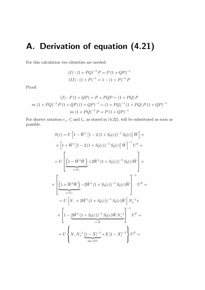
A. Derivation of equation (4.21)

For this calculation two identities are needed:

(I) : (1 + PQ)−1 P = P (1 +QP )−1

(II) : (1 + P )−1 = 1− (1 + P )−1 P

Proof:

(I) : P (1 +QP ) = P + PQP = (1 + PQ)P

⇔ (1 + PQ)−1 P (1 +QP ) (1 +QP )−1 = (1 + PQ)−1 (1 + PQ)P (1 +QP )−1

⇔ (1 + PQ)−1 P = P (1 +QP )−1

For shorter notation rc, r′c and tc, as stated in (4.22), will be substituted as soon as

possible.

S(ε) = U[1− W † [1− 2 (1 + S0(ε))−1 S0(ε)

]W]×

×[1 + W † [1− 2 (1 + S0(ε))−1 S0(ε)

]W]−1

UT =

= U

(1− W †W)

︸ ︷︷ ︸=:N−

+2W † (1 + S0(ε))−1 S0(ε)W

×

×

(1 + W †W)

︸ ︷︷ ︸=:N+

−2W † (1 + S0(ε))−1 S0(ε)W

−1

UT =

= U[N− + 2W † (1 + S0(ε))−1 S0(ε)W

]N−1

+ ×

×

1− 2W † (1 + S0(ε))−1 S0(ε)WN−1+︸ ︷︷ ︸

=:X

−1

UT =

= U

N−N−1+ [1−X]−1︸ ︷︷ ︸

use (II)

+X [1−X]−1

UT =

36 A. Derivation of equation (4.21)

= U{N−N

−1+

(1 + [1−X]−1X

)+X (1−X)−1}UT =

= U{N−N

−1+ +

(N−N

−1+ + 1

)[1−X]−1X

}UT =

= UN−N−1+ UT︸ ︷︷ ︸

=rc

+UT (N− +N+)︸ ︷︷ ︸=2

N−1+

[1− 2W † (1 + S0(ε))−1 S0(ε)WN−1

+

]−1

W †︸ ︷︷ ︸use (I)with P=W †

×

× (1 + S0(ε))−1 S0(ε) W2N−1+ U︸ ︷︷ ︸

=tc

=

= rc + UT2N−1+ W †︸ ︷︷ ︸

=tTc

[1− 2 (1 + S0(ε))−1 S0(ε)WN−1

+ W †]−1

(1 + S0(ε))−1 S0(ε)tc =

= rc + tTc

[1 + S0(ε)− 2S0(ε)WN−1

+ W †]−1

S0(ε)tc =

= rc + tTc

[1 + S0(ε)

(1− 2WN−1

+ W †)]−1

S0(ε)tc =

(I)= rc + tTc S0(ε)

[1 +

(WN+N

−1+ W−1 − 2WN−1

+ W †WW−1)S0(ε)

]−1

tc =

= rc + tTc S0(ε)[1 + W

(N+N

−1+ − 2N−1

+ W †W)W−1S0(ε)

]−1

tc =

= rc + tTc S0(ε)

1 + W(N+ − 2W †W

)︸ ︷︷ ︸

=N−

N−1+ W−1S0(ε)

−1

tc =

= rc + tTc S0(ε)

1−(−WN−N

−1+ W−1

)︸ ︷︷ ︸

=r′c

S0(ε)

−1

tc =

= rc + tTc S0(ε) [1− r′cS0(ε)]−1tc

B. Code for the random matrixHamiltonian

1 %number o f channe l s in the dot2 M = 50 ;34 %number o f i n t e r v a l s f o r the historgram of a l l e i g e n v a l u e s5 res = 500 ;67 %number o f d i s o r d e r r e a l i z a t i o n s8 L = 10000;9

10 %number o f randomly picked r e a l i z a t i o n s p l o t t e t in one f i g u r e11 nall = 5 ;1213 %number o f randomly picked r e a l i z a t i o n s p l o t t e t in d i s t i n c t f i g u r e s14 nsin = 5 ;1516 %r e f e l c t i o n ampl itudes o f the QPC17 r = [−0.1 −0 .3 ] ;1819 %c a l c u l a t e s e l f e n e r g y part20 d = size ( r ) ;21 W2 = zeros ( M ) ;22 for m=1:d (2 )23 W2 (m , m ) = (1+r ( m ) ) /(1−r ( m ) ) ;24 end

2526 %c a l c u l a t e imagniary par t s o f the e i g e n v a l u e s in un i t s o f mean l e v e l s p a c i n g f o r ←↩

a l l r e a l i z a t i o n s27 data = zeros ( L∗M , 1 ) ;28 delta = 0 ;29 gamma = 0 ;30 for k=1:L31 A = normrnd (0 , 1 , M , M ) ;32 H = triu ( A )+(triu (A , 1 ) . ' ) +1i∗W2 ;33 lambda = ( eig ( H ) ) . ' ;34 gamma = gamma + imag ( sum ( lambda ) ) /M ;35 data ( ( k−1)∗M+1:k∗M ) = imag ( lambda ) ;36 delta = delta + ( max ( real ( lambda ) )−min ( real ( lambda ) ) ) /M ;37 end

3839 gamma = gamma/L ;40 delta = delta/L ;41 data_mls = data/delta ;42 [ n , x ]=hist ( data_mls , res ) ;43 delta_x = x (2 ) − x (1 ) ;4445 %plo t s t a t i s t i c o f a l l r e a l i s a t i o n s46 figure

47 bar (x , n/sum ( n∗delta_x ) , 'hist' ) ;48 set ( gca , 'FontSize ' , 30) ;49 title ( sprintf ( 'r_1=%g, r_2=%g, L=%g, M=%g, \\ Gamma /\\ Delta =%0.2g' , r (1 ) , r (2 ) ,L , M ,←↩

gamma/delta ) ) ;

38 B. Code for the random matrix Hamiltonian

50 ylabel ( 'normalized number of occurences ' ) ;51 xlabel ( '\gamma/\Delta ' ) ;52 legend ( sprintf ( 'bar width=%g' , delta_x ) ) ;535455 %plo t s i n g l e randomly taken r e a l i s a t i o n s in d i f f e r e n t p l o t s56 rsin = randi (L , nsin , 1 ) ;5758 for z=1:nsin59 figure

60 pic = sort ( data_mls ( M∗rsin ( z )−M+1:M∗rsin ( z ) ) ) ;61 stem ( pic ) ;62 set ( gca , 'FontSize ' , 30) ;63 title ( sprintf ( 'r_1=%g, r_2=%g, M=%g, \\Gamma /\\ Delta =%0.2g' , r (1 ) , r (2 ) ,M , gamma←↩

/delta ) ) ;64 xlabel ( '\gamma sorted by size' ) ;65 ylabel ( '\gamma/\Delta ' ) ;66 set ( gca , 'XTickLabelMode ' , 'manual ' , 'XTickLabel ' , [ ] ) ;67 end

6869 %plo t randomly taken r e a l i s a t i o n s in to one p l o t70 rall = randi (L , nall , 1 ) ;7172 figure

73 set ( gca , 'FontSize ' , 30) ;74 title ( sprintf ( 'r_1=%g, r_2=%g, M=%g, \\Gamma /\\ Delta =%0.2g, %g Realizations ' , r (1 )←↩

, r (2 ) ,M , gamma/delta , nall ) ) ;75 xlabel ( '\gamma sorted by size' ) ;76 ylabel ( '\gamma/\Delta ' ) ;77 set ( gca , 'XTickLabelMode ' , 'manual ' , 'XTickLabel ' , [ ] ) ;7879 hold all

8081 for zall=1:nall82 pic = sort ( data_mls ( M∗rall ( zall )−M+1:M∗rall ( zall ) ) ) ;83 stem ( pic ) ;84 end

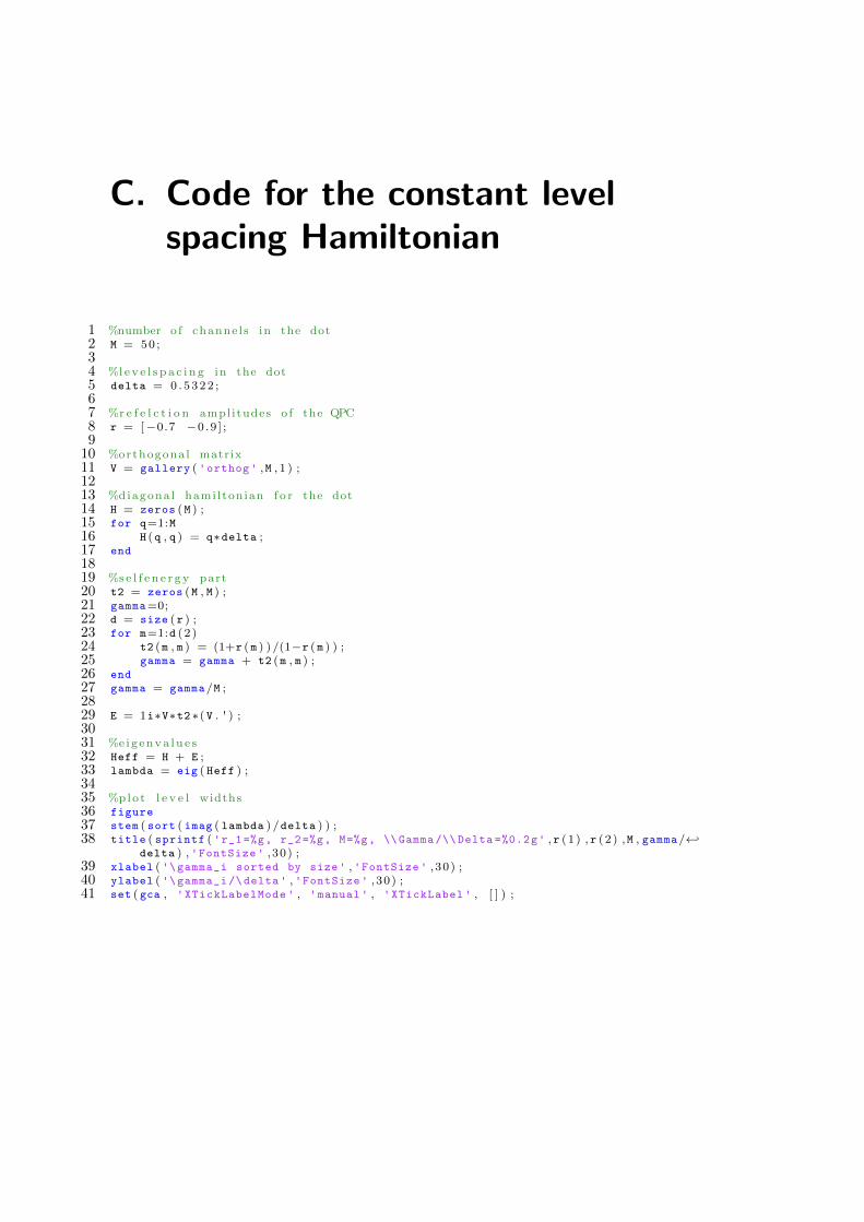
C. Code for the constant levelspacing Hamiltonian

1 %number o f channe l s in the dot2 M = 50 ;34 %l e v e l s p a c i n g in the dot5 delta = 0 . 5 3 2 2 ;67 %r e f e l c t i o n ampl itudes o f the QPC8 r = [−0.7 −0 .9 ] ;9

10 %orthogona l matrix11 V = gallery ( 'orthog ' ,M , 1 ) ;1213 %diagona l hami l tonian f o r the dot14 H = zeros ( M ) ;15 for q=1:M16 H (q , q ) = q∗delta ;17 end

1819 %s e l f e n e r g y part20 t2 = zeros (M , M ) ;21 gamma=0;22 d = size ( r ) ;23 for m=1:d (2 )24 t2 (m , m ) = (1+r ( m ) ) /(1−r ( m ) ) ;25 gamma = gamma + t2 (m , m ) ;26 end

27 gamma = gamma/M ;2829 E = 1i∗V∗t2 ∗( V . ' ) ;3031 %e i g e n v a l u e s32 Heff = H + E ;33 lambda = eig ( Heff ) ;3435 %plo t l e v e l widths36 figure

37 stem ( sort ( imag ( lambda ) /delta ) ) ;38 title ( sprintf ( 'r_1=%g, r_2=%g, M=%g, \\Gamma /\\ Delta =%0.2g' , r (1 ) , r (2 ) ,M , gamma/←↩

delta ) , 'FontSize ' , 30) ;39 xlabel ( '\gamma_i sorted by size' , 'FontSize ' , 30) ;40 ylabel ( '\gamma_i /\ delta' , 'FontSize ' , 30) ;41 set ( gca , 'XTickLabelMode ' , 'manual ' , 'XTickLabel ' , [ ] ) ;

Bibliography

[1] J. Feldmann, lecture notes on ”Advanced Solid State Physics”, LMU(2013/14).

[2] I.L. Aleiner, P.W. Brouwer, L.I. Glazman, Physics Reports 358 (2002), pp.309-440.

[3] J. von Delft, lecture notes on ”Mesoscopics”, LMU (2013).

[4] Y. Yacoby et al., Phys. Rev. Lett. 74, 4047 (1995).

[5] S. Datta, Electronic Transport in Mesoscopic Systems (Cambridge UniversityPress, New York, 1995).

[6] R. Schuster et al., Nature (London) 385, 417 (1997).

[7] M. Avinun-Khalish et al., Nature (London) 436, 529 (2005).

[8] C. Karrasch, T. Hecht, A. Weichselbaum, Y. Oreg, J. von Delft, V. Meden,Phys. Rev. Lett 98, 186802 (2007).

[9] Yuli V. Nazarov, Yaroslav M. Blanter, Quantum Transport (Cambridge Uni-versity Press, New York, 2009).

[10] T. Hecht, A. Weichselbaum, Y. Oreg, J. von Delft, Phys. Rev. B 80, 115330(2009).

[11] I.L.Kurland, I.L. Aleiner, B.L. Altshuler, Phys. Rev. B 62, 14886 (2000).

[12] P.W. Brouwer, Phys. Rev. B 51, 16878 (1995).

[13] U. Fano, Phys. Rev. 124, 1866 (1961).

[14] M.L. Mehta, Random Matrices (Elsevier Academic Press, Amsterdam, 2004).

[15] A.L. Fetter, J.D. Walecka, Quantum Theory of Many-Particle Systems (DoverPublications, New York, 1971).

[16] C. Karrasch, T. Hecht, A. Weichselbaum, Y. Oreg, J. von Delft, V. Meden,New Journal pf Physics 9, (2007) 123.

[17] A. Altland, B. Simons, Condensed Matter Field Theory (Cambridge UniversityPress, New York, 2006).

Acknowledgements

I want to thank Dr. Oleg Yevtushenko for introducing me to the field of electron

transport in mesoscopic systems and giving me the chance to work on this subject.

He guided me patiently in this thesis with explanations and discussions. Furthermore

his helping hand in correcting mistakes and proof reading my thesis was very valuable

and I am very grateful for that.

I also want to thank Prof. Jan von Delft for looking into the problem when we got

stuck.

Statutory Declaration

I declare on oath that I completed this work on my own and that information which

has been directly or indirectly taken from other sources has been noted as such.

Neither this, nor a similar work, has been published or presented to an examination

committee.

Munich, December 20, 2013

Place, Date signature