Transportation Research Part A 88 (2016) 209–222

Contents lists available at ScienceDirect

Transportation Research Part A

journal homepage: www.elsevier .com/locate / t ra

Feeder-trunk or direct lines? Economies of density, transfercosts and transit structure in an urban context

http://dx.doi.org/10.1016/j.tra.2016.03.0010965-8564/� 2016 Elsevier Ltd. All rights reserved.

⇑ Corresponding author.E-mail address: jaradiaz@ing.uchile.cl (S. Jara-Díaz).

1 This was indeed the argument behind the route structure introduced in Santiago, Chile, in 2007 (Díaz et al., 2002).

Antonio Gschwender, Sergio Jara-Díaz ⇑, Claudia BravoUniversidad de Chile, Chile

a r t i c l e i n f o a b s t r a c t

Article history:Received 7 May 2015Received in revised form 1 October 2015Accepted 1 March 2016Available online 29 April 2016

Keywords:Public transportOptimal lines structureFeeder-trunkDirect linesEconomies of density

A feeder-trunk scheme has been labeled as superior in urban areas due to the presence ofeconomies of density (decreasing average operating cost) along the avenues served bytrunk lines. We compare this structure against three types of direct lines structures(no transfers) to serve a stylized public transport network where several flows convergeinto a main avenue, simultaneously optimizing fleet and vehicle sizes considering bothusers’ and operators’ costs. The best structure is shown to depend not only on the totalpassenger volume but also on demand imbalance, demand dispersion in the origins andthe length of the trunk line. The region where the feeder-trunk structure dominatesdepends largely on the value assigned to the pure transfer penalty.

� 2016 Elsevier Ltd. All rights reserved.

1. Introduction

In most Latin American urban areas the proportion of users of public transport systems is similar to (and sometimes lar-ger than) those observed in European ones. At the beginning of the 21st century many Latin American systems exhibited alarge fleet of badly maintained buses operating over long routes that crossed the CBD and overlapped in the main avenues ofthe urban area, providing direct services for most of the users. This induced the introduction of different types of reforms.Some cities have implemented a systemwith a smaller fleet of larger buses in average, organized under a feeder-trunk routesstructure. The case for a feeder-trunk system rests on the so-called economies of density, a property of a transport cost func-tion understood in this case as the savings in operating costs that can be achieved by using large (cheaper per passenger)vehicles in the main streets or avenues that receive passengers from many possible feeder lines using smaller vehicles.Therefore, this structure seems attractive because of the flexibility of the different fleets in terms of number of vehiclesand vehicle sizes.1

Savings in operating costs are only one part of the picture. The feeder-trunk scheme induces mandatory transfers at everyconnecting point where the feeder lines meet the trunk lines. Transfers not only cause additional waiting and walking timesbut also imply the interruption of the trip – which we will call disruption – that has been shown to be unpleasant by itself(Currie, 2005); simultaneously, though, frequencies on the trunk lines are likely to be high such that additional waiting couldbe small. There are alternative schemes that avoid the mandatory transfers; the most evident one is a system of point-to-point or direct lines that would overlap along the main streets. These direct services could be conceived in various ways;for example, with all lines departing from the origin points in the local streets and then collecting passengers along the main

210 A. Gschwender et al. / Transportation Research Part A 88 (2016) 209–222

avenues. In this case, the need to generate capacity to accommodate the flows originated along the main avenues wouldinduce idle capacity in the vehicles when traveling along the local streets, inducing higher costs for the operators. This effectcould be diminished by providing additional services starting at the main avenues themselves.

Many lines structures can be imagined, each one presenting advantages and disadvantages for users and operators. Eachalternative would imply different characteristics regarding other design variables, as frequency and vehicle size of each ofthe fleets required. The appropriate values for these variables and for the most adequate spatial structure of services willin turn depend on whether flows originate mostly in the local streets (relatively long trips) or in the main avenues (relativelyshort trips). In this paper we present an analytical framework using a simple network graph in order to analyze under whichcircumstances a feeder-trunk scheme is superior to other options, taking into account explicitly the presence of a collectingpoint where several local flows converge, and thus allowing economies of density to arise. In addition, the effects of the totalpassenger volume and the relative amount of long trips (which we call imbalance) are examined, considering the possibleimpact of a pure transfer penalty. From an economic viewpoint we will follow a social cost function approach, where thetotal resources consumed including users time is minimized for a parametrically given demand.2 In the next section we pre-sent a simple network and a parametrical formulation of the demand structure that permits the introduction of all the relevantaspects; we also define the service structures that will be analyzed. In the third section we formulate the general cost minimiz-ing problem (users and operators) parametrically in the imbalance between short and long trips and in the total demand, whichis then solved for each structure obtaining the optimal design variables; in the base case, transfers are considered only throughadditional waiting time. Then we discuss the reasons behind the superiority of the best structure for different imbalances andpassenger volume combinations. In Section 5 we depart from the base case to study the effect of a key parameter, namely thetransfer penalty (disruption and walking). In Section 6 the effects of two spatial parameters – length of the avenue and demanddispersion in the origins – are explored. Conclusions are offered in the final section.

2. Problem formulation

The specific problem of a choice between feeder-trunk and other structures has been discussed, for example, by Sandoval(2010) who compared feeder-trunk systems within the Bus Rapid Transit scheme in several developing cities, suggestingthat service level could be improved by making the system less rigid allowing direct lines as well. In another case study,El-Hifnawi (2002) analyzed the economic impact of the implementation of direct lines crossing the urban area of Monterrey,Mexico. According to Kepaptsoglou and Karlaftis (2009), the choice on an appropriate lines structure can be approached fromtwo perspectives: heuristics and analytical. Heuristics have been developed to help with the design of real size transit sys-tems, while the analytical approach has proved useful to provide a starting point for a detailed design. As Ceder (2001) pointsout, analytical modeling on simple networks is helpful both for the strategic design of real transit networks and for policyanalyses. Within this perspective simplicity has two connotations. One is the analysis of regular or symmetric networks as inKocur and Hendrickson (1982) and Chang and Schonfeld (1991) who analyzed the spacing of parallel lines; Aldaihani et al.(2004), who extended this to a grid plus a demand responsive feeder system; Jara-Díaz et al. (2014), who used a cross-shapednetwork to analyze the impact of ignoring users’ cost when comparing direct lines against rigid corridor-lines; Tirachini et al.(2010), who analyzed a radial system; or Daganzo (2010), Estrada et al. (2011) and Badia et al. (2014), who studied a squared,rectangular and radial system respectively, with a hybrid lines structure. A second idea of simplicity is present in the analysisof stylized (small) networks with a precise intention, as in Brueckner (2004), who used a triangle-shaped three nodes net-work to compare fully connected versus hub and spoke lines structures in air transport; Jara-Díaz et al. (2012), who analyzeda one dimensional corridor with two origins and one common destination with imbalance as the only flow-related variable;or Quadrifoglio and Li (2011), who developed a model to choose between a fixed feeder system and a demand responsiveone. In this paper we follow the second idea of simplicity, explicitly incorporating the effects of collecting flows at a pointand the presence of a transfer penalty.

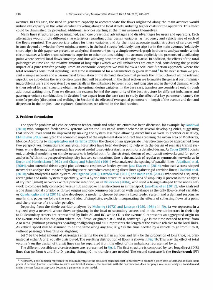
Departing from the single corridor analyses by Mohring (1972) and Jansson (1980, 1984), in Fig. 1a we represent in astylized way a network where flows originating in the local or secondary streets and in the avenue interact in their tripto D. Secondary streets are represented by links AC and BC, while CD is the avenue. C represents an aggregated origin onthe avenue and is also the point where local flows, originated at A and B, converge. T1/2 is the time needed to travel fromA or B to C (without passengers boarding or alighting) and n > 1 represents the length of the avenue relative to the local links.As vehicle speed will be assumed to be the same along any link, nT1/2 is the time needed by a vehicle to go from C to D,without passengers boarding or alighting.

Let Y be the total amount of passengers entering the system in an hour and let a be the proportion of long trips, i.e. orig-inated at either A or B, equally distributed. The resulting distribution of flows is shown in Fig. 1b. This way the effect of totalvolume Y on the design of transit lines can be separated from the effect of the imbalance represented by a.

The different possible service structures are represented in Fig. 2. The first structure is composed by two long direct (DIR)lines that go from A and B to D, passing through C; no transfers are needed. The second structure is the feeder-trunk (FT)

2 As known, a cost function represents the minimum value of the resources consumed that is necessary to produce a given level of demand at given inputprices. A demand function – sensitive to prices and level of service – that interacts with the cost function, does not play a role in our analysis; total demandunder the cost function approach becomes a parameter in our model.

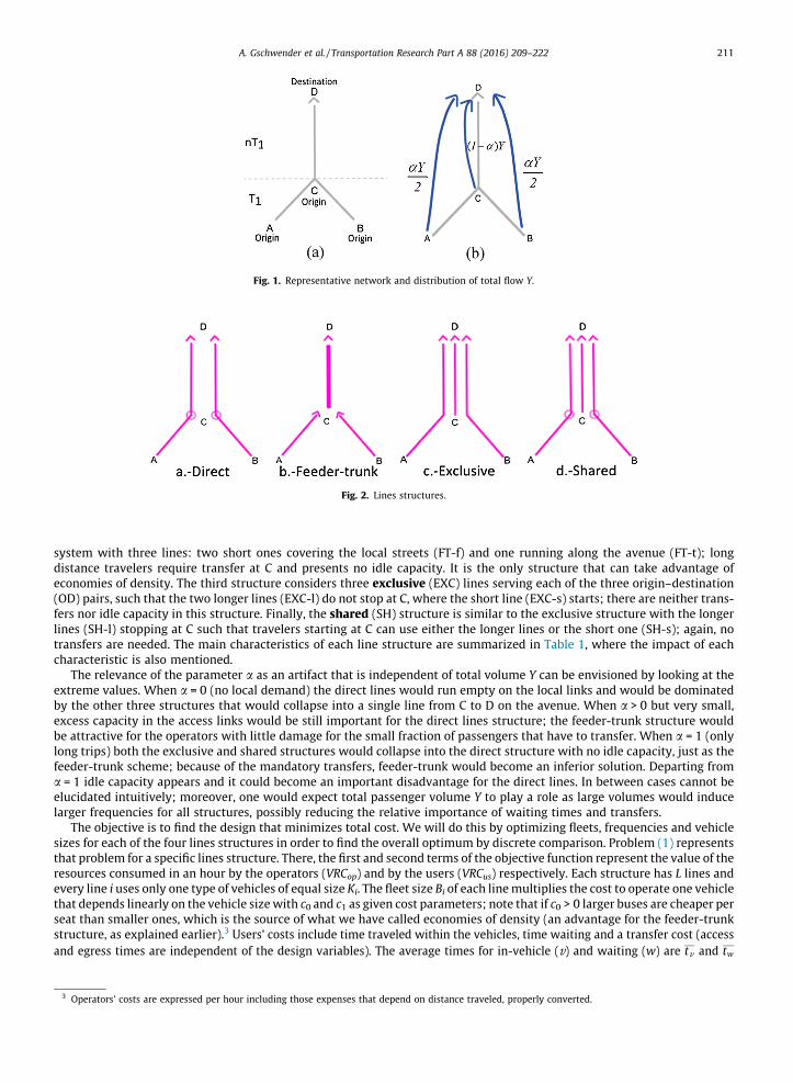
Fig. 1. Representative network and distribution of total flow Y.

Fig. 2. Lines structures.

A. Gschwender et al. / Transportation Research Part A 88 (2016) 209–222 211

system with three lines: two short ones covering the local streets (FT-f) and one running along the avenue (FT-t); longdistance travelers require transfer at C and presents no idle capacity. It is the only structure that can take advantage ofeconomies of density. The third structure considers three exclusive (EXC) lines serving each of the three origin–destination(OD) pairs, such that the two longer lines (EXC-l) do not stop at C, where the short line (EXC-s) starts; there are neither trans-fers nor idle capacity in this structure. Finally, the shared (SH) structure is similar to the exclusive structure with the longerlines (SH-l) stopping at C such that travelers starting at C can use either the longer lines or the short one (SH-s); again, notransfers are needed. The main characteristics of each line structure are summarized in Table 1, where the impact of eachcharacteristic is also mentioned.

The relevance of the parameter a as an artifact that is independent of total volume Y can be envisioned by looking at theextreme values. When a = 0 (no local demand) the direct lines would run empty on the local links and would be dominatedby the other three structures that would collapse into a single line from C to D on the avenue. When a > 0 but very small,excess capacity in the access links would be still important for the direct lines structure; the feeder-trunk structure wouldbe attractive for the operators with little damage for the small fraction of passengers that have to transfer. When a = 1 (onlylong trips) both the exclusive and shared structures would collapse into the direct structure with no idle capacity, just as thefeeder-trunk scheme; because of the mandatory transfers, feeder-trunk would become an inferior solution. Departing froma = 1 idle capacity appears and it could become an important disadvantage for the direct lines. In between cases cannot beelucidated intuitively; moreover, one would expect total passenger volume Y to play a role as large volumes would inducelarger frequencies for all structures, possibly reducing the relative importance of waiting times and transfers.

The objective is to find the design that minimizes total cost. We will do this by optimizing fleets, frequencies and vehiclesizes for each of the four lines structures in order to find the overall optimum by discrete comparison. Problem (1) representsthat problem for a specific lines structure. There, the first and second terms of the objective function represent the value of theresources consumed in an hour by the operators (VRCop) and by the users (VRCus) respectively. Each structure has L lines andevery line i uses only one type of vehicles of equal size Ki. The fleet size Bi of each linemultiplies the cost to operate one vehiclethat depends linearly on the vehicle sizewith c0 and c1 as given cost parameters; note that if c0 > 0 larger buses are cheaper perseat than smaller ones, which is the source of what we have called economies of density (an advantage for the feeder-trunkstructure, as explained earlier).3 Users’ costs include time traveled within the vehicles, time waiting and a transfer cost (accessand egress times are independent of the design variables). The average times for in-vehicle (v) and waiting (w) are tv and tw

3 Operators’ costs are expressed per hour including those expenses that depend on distance traveled, properly converted.

Table 1Main characteristics of the lines structures.

Idle capacity Transfers Economies of density

Direct (DIR) Yes No NoFeeder-trunk (FT) No Yes YesExclusive (EXC) No No NoShared (SH) Yes No No

Impact Increases operators’ costs Increases waiting timeIncreases cycle time (op. costs)Increases in-vehicle time

Diminishes operators’ costs

212 A. Gschwender et al. / Transportation Research Part A 88 (2016) 209–222

respectively; Pv and Pw are the associated values of time. The treatment of transfer cost will be discussed later, with g theproportion of users that has to transfer in that specific line structure. A glossary of variables is included in Appendix A.

min VRC ¼ VRCop þ VRCus ¼XL

i¼1

Biðc0 þ c1KiÞ þ YðPv tv þ Pwtw þ PtgÞ

subject to ki ¼ kif i6 Ki

ð1Þ

The constraint in (1) imposes that vehicle capacity has to be large enough to carry the maximum vehicle load ki given by theratio between the maximum flow of the line, ki, and its frequency fi. Note that the maximum flow is independent of thedesign variables for each line within a given line structure. As will be confirmed later, neither in-vehicle nor waiting timesdepend on Ki directly; same with g. Then the constraint is always active as cost increases with Ki. As fleet sizes, bus capac-ities, waiting and in-vehicle times can always be expressed as functions of frequencies, problem (1) can be solved for eachand every lines structure with frequencies as the optimization variables. Note that Ki itself has an upper limit within a giventechnology (bus); feasibility should be verified after a numerical result has been obtained.

In our model we will assume that boarding and alighting occurs sequentially at all available doors with an explicit impacton cycle and in-vehicle times (see Eq. (2) and its explanation in the next section). Also, there is no bus schedule as such andwaiting time will be a proportion e of the headway (see Eq. (5) below). If buses and passengers arrive regularly e = 0.5(assumed in the numerical simulations).

3. Finding the optimal structures in the base scenario

In this section we will solve problem (1) for each of the four cases identified previously and then we will find the overalloptimum through discrete comparisons parametrically in Y and a. Three of the cases can be solved analytically and one – thecase of shared lines – has to be solved numerically as will be explained later. In the base scenario we will assume that trans-fers affect users only through additional waiting time; the very important effect of additional walking and disruption of thetrip will be specifically analyzed in Section 5.

Let us illustrate the analytical procedure with the case of direct lines. In Fig. 3 we show the boarding and alighting patterncorresponding to the assignment of passengers described in Fig. 1b to one of the two symmetric direct lines defined in Fig. 2.This pattern results in a maximum flow of Y/2 for each direct line in the main street.

Given the symmetry of the problem, the VRCop adds up over two identical lines; for this reason we omit the subscript i. Oneach line the fleet size and the frequency are related through B ¼ f � TC where TC is cycle time of one vehicle, which includesthe time vehicle is in motion (first term in Eq. (2)) and total boarding and alighting time (second term, where t is the averagetime a vehicle has to stop to let one passenger board or alight).

TC ¼ ðnþ 1ÞT1 þ 2taY2

þ ð1� aÞY2

� �1f¼ ðnþ 1ÞT1 þ tY

fð2Þ

From this B can be written as a function of f as

B ¼ f ðnþ 1ÞT1 þ tY ð3Þ

As the capacity constraint is always active, K is given by the ratio between the maximum flow Y/2 and f; then VRCop as afunction of f only is given by

VRCop ¼ 2 c0 þ c1Y2f

� �½f ðnþ 1ÞT1 þ tY� ð4Þ

Regarding users’ costs a proportion a of users (long trips) experience a waiting time of e/f and the remaining 1 � a users,starting at C, experience half of this as they see two identical services. Therefore average waiting time is

tw ¼ efaþ e

2fð1� aÞ ð5Þ

Fig. 3. Boarding, alighting and arc flows for a direct line.

A. Gschwender et al. / Transportation Research Part A 88 (2016) 209–222 213

The same proportions are applicable to calculate average in-vehicle time. In addition to time in motion, the aY users board-ing at A and B have to stay on the vehicle while (1 � a)Y/2 users board at C and then have to alight at D. Therefore, in-vehicletime for users boarding at A and B is

tABv ¼ ðnþ 1ÞT1

2þ t

ð1� aÞY2f

� �þ t2

ð1� aÞ2

þ a2

� �Yf¼ ðnþ 1ÞT1

2þ ð3� 2aÞ

4tYf

ð6Þ

The remaining passengers that board at C have a shorter time in motion and the same alighting time at D, which yields

tCv ¼ nT1

2þ t2

ð1� aÞ2

þ a2

� �Yf¼ nT1

2þ tY4f

ð7Þ

Weighting in-vehicle time (6) and (7) by a and (1 � a) respectively the average in-vehicle time is

tv ¼ ðnþ aÞT1

2þ ð1� 2a2 þ 2aÞ tY

4fð8Þ

Then the VRCus is

VRCus ¼ Pw � eð1þ 2a� aÞ2f

� �� Y þ Pv � ðnþ aÞT1

2þ ð1� 2a2 þ 2aÞ tY

4f

� �� Y ð9Þ

Now both operators and users costs are written as a function of frequency. Minimizing the sum of Eqs. (4) and (9) withrespect to f yields the optimal frequency for each of the direct lines

f �DIR ¼ffiffiffiffiffiffiffiffiffiffiffiffiffiffiffiffiffiffiffiffiffiffiffiffiffiffiffiffiffiffiffiffiffiffiffiffiffiffiffiffiffiffiffiffiffiffiffiffiffiffiffiffiffiffiffiffiffiffiffiffiffiffiffiffiffiffiffiffiffiffiffiffiffiffiffiffiffiffiffiffiffiffiffiffiffiffiffiffiffiffiffiffiffiffiffiffiffiffiffiffiffiffiffiffiffiffiffiffiffiffiffiffiffiffiffiffiffiffiffiffiffiffi

Y8c0ð1þ nÞT1

½4c1tY þ 2Pweð1þ aÞ þ Pv tYð1� 2a2 þ 2aÞ�s

ð10Þ

The resulting minimum cost is

VRC�DIR ¼ 2tYc0 þ

ffiffiffiffiffiffiffiffiffiffiffiffiffiffiffiffiffiffiffiffiffiffiffiffiffiffiffiffiffiffiffiffiffiffiffiffiffiffiffiffiffiffiffiffiffiffiffiffiffiffiffiffiffiffiffiffiffiffiffiffiffiffiffiffiffiffiffiffiffiffiffiffiffiffiffiffiffiffiffiffiffiffiffiffiffiffiffiffiffiffiffiffiffiffiffiffiffiffiffiffiffiffiffiffiffiffiffiffiffiffiffiffiffiffiffiffiffiffiffiffiffiffiffiffi2ð1þ nÞT1Yc0½4c1tY þ 2ð1þ aÞePw þ ð1� 2a2 þ 2aÞPv tY�

qþ T1Y c1ðnþ 1Þ þ Pv

2ðnþ aÞ

� �ð11Þ

Following the same procedure we solved the feeder-trunk structure that yields two optimal frequencies, one for each of thetwo identical feeder lines and one for the trunk line. The results are

f �FT-f ¼ffiffiffiffiffiffiffiffiffiffiffiffiffiffiffiffiffiffiffiffiffiffiffiffiffiffiffiffiffiffiffiffiffiffiffiffiffiffiffiffiffiffiffiffiffiffiffiffiffiffiffiffiffiffiffiffiffiffiffiffiffiffiffiffiffiffiffiaY

8T1c0ð4ac1tY þ 4ePw þ PvatYÞ

sð12Þ

f �FT-t ¼ffiffiffiffiffiffiffiffiffiffiffiffiffiffiffiffiffiffiffiffiffiffiffiffiffiffiffiffiffiffiffiffiffiffiffiffiffiffiffiffiffiffiffiffiffiffiffiffiffiffiffiffiffiffiffiffiffiffiffiffiffiffiffiffi

Y2nT1c0

ð4c1tY þ 2ePw þ Pv tYÞs

ð13Þ

VRC�FT ¼ 2tYc0ð1þ aÞ þ

ffiffiffiffiffiffiffiffiffiffiffiffiffiffiffiffiffiffiffiffiffiffiffiffiffiffiffiffiffiffiffiffiffiffiffiffiffiffiffiffiffiffiffiffiffiffiffiffiffiffiffiffiffiffiffiffiffiffiffiffiffiffiffiffiffiffiffiffiffiffiffiffi2YT1ac0ð4ac1tY þ 4ePw þ PvatYÞ

pþ

ffiffiffiffiffiffiffiffiffiffiffiffiffiffiffiffiffiffiffiffiffiffiffiffiffiffiffiffiffiffiffiffiffiffiffiffiffiffiffiffiffiffiffiffiffiffiffiffiffiffiffiffiffiffiffiffiffiffiffiffiffiffiffiffiffiffi2nT1Yc0ð4c1tY þ 2ePw þ Pv tYÞ

pþ T1Yðnþ aÞ c1 þ Pv

2

� �ð14Þ

Similarly, the result for the exclusive structure also involves two frequencies, one for the two identical longer lines and onefor the shorter one. Results are

214 A. Gschwender et al. / Transportation Research Part A 88 (2016) 209–222

f �EXC-l ¼ffiffiffiffiffiffiffiffiffiffiffiffiffiffiffiffiffiffiffiffiffiffiffiffiffiffiffiffiffiffiffiffiffiffiffiffiffiffiffiffiffiffiffiffiffiffiffiffiffiffiffiffiffiffiffiffiffiffiffiffiffiffiffiffiffiffiffiffiffiffiffiffiffiffiffiffiffiffiffiffiffiffi

aY8ðnþ 1ÞT1c0

ð4ac1tY þ 4ePw þ aPv tYÞs

ð15Þ

f �EXC-s ¼ffiffiffiffiffiffiffiffiffiffiffiffiffiffiffiffiffiffiffiffiffiffiffiffiffiffiffiffiffiffiffiffiffiffiffiffiffiffiffiffiffiffiffiffiffiffiffiffiffiffiffiffiffiffiffiffiffiffiffiffiffiffiffiffiffiffiffiffiffiffiffiffiffiffiffiffiffiffiffiffiffiffiffiffiffiffiffiffiffiffiffiffiffiffiffiffiffiffið1� aÞY2nT1c0

ð4ð1� aÞc1tY þ 2ePw þ ð1� aÞPv tYÞs

ð16Þ

VRC�EXC ¼ 2tYc0 þ

ffiffiffiffiffiffiffiffiffiffiffiffiffiffiffiffiffiffiffiffiffiffiffiffiffiffiffiffiffiffiffiffiffiffiffiffiffiffiffiffiffiffiffiffiffiffiffiffiffiffiffiffiffiffiffiffiffiffiffiffiffiffiffiffiffiffiffiffiffiffiffiffiffiffiffiffiffiffiffiffiffiffiffiffiffiffiffi2ð1þ nÞac0T1Yð4ac1tY þ 4ePw þ aPv tYÞ

pþ

ffiffiffiffiffiffiffiffiffiffiffiffiffiffiffiffiffiffiffiffiffiffiffiffiffiffiffiffiffiffiffiffiffiffiffiffiffiffiffiffiffiffiffiffiffiffiffiffiffiffiffiffiffiffiffiffiffiffiffiffiffiffiffiffiffiffiffiffiffiffiffiffiffiffiffiffiffiffiffiffiffiffiffiffiffiffiffiffiffiffiffiffiffiffiffiffiffiffiffiffiffiffiffiffiffiffiffiffiffiffiffiffi2ð1� aÞc0nT1Yð4ð1� aÞc1tY þ 2ePw þ ð1� aÞPv tYÞ

pþ T1Yðaþ nÞðc1 þ Pv=2Þ ð17Þ

In the case of the shared lines, passengers going from junction C to destination D can board any of the three lines, i.e. thosecoming from A or B and the line that starts at C. Therefore, the amount of passengers boarding each line depends on allfrequencies. This makes the cycle time of each fleet dependent on the frequencies of both types of lines, short and long.As a result, the fleet sizes (given by frequency times cycle time) are also dependent on both frequencies, as shown byEqs. (18) and (19).

BSH-l ¼ f SH-lðnþ 1ÞT1 þ 2tYa2þ ð1� aÞf SH-l

ð2f SH-l þ f SH-sÞ� �

ð18Þ

BSH-s ¼ f SH-snT1 þ 2tYð1� aÞf SH-s

ð2f SH-l þ f SH-sÞð19Þ

This yields a value of the resources consumed for the shared lines that depends on fSH-l and fSH-s in a complex way as shownin Eq. (20) where BSH-l and BSH-s corresponds to Eqs. (18) and (19). As in Jara-Díaz et al. (2012), the problem cannot be solvedanalytically and has to be faced numerically.

VRCSH ¼ 2 c0 þ c1aY

2f SH-lþ ð1� aÞY2f SH-l þ f SH-s

� �� �BSH-l þ c0 þ c1

ð1� aÞY2f SH-l þ f SH-s

� �� �BSH-s

þ Pe ea

f SH-lþ ð1� aÞ2f SH-l þ f SH-s

� �� �Y þ Pv

ðaþ nÞT1

2þ tYð1� 2aða� 1ÞÞ

2ð2f SH-l þ f SH-sÞþ a2f SH-stY4f SH-lð2f SH-l þ f SH-sÞ

� �Y ð20Þ

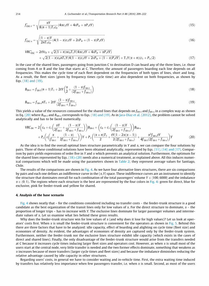
As the idea is to find the overall optimal lines structure parametrically in Y and a, we can compare the four solutions bypairs. Three of these conditional solutions have been obtained analytically, represented by Eqs. (11), (14) and (17). Compar-ison by pairs yields expressions of order five in Y and a which prevents an analytical solution. Furthermore, the optimum forthe shared lines represented by Eqs. (18)–(20) needs also a numerical treatment, as explained above. All this induces numer-ical comparisons which will be made using the parameters shown in Table 2; they represent average values for Santiago,Chile.

The results of the comparisons are shown in Fig. 4. As we have four alternative lines structures, there are six comparisonsby pairs and each one defines an indifference curve in the (a,Y) space. These indifference curves are an instrument to identifythe structure that dominates overall for each combination of the total passengers’ volume Y 2 ½100;6000� and the imbalancea 2 ð0;1Þ. The regions where each structure is the best are represented by the four colors in Fig. 4: green for direct, blue forexclusive, pink for feeder-trunk and yellow for shared.

4. Analysis of the base scenario

Fig. 4 shows neatly that – for the conditions considered including no transfer costs – the feeder-trunk structure is a goodcandidate as the best organization of the transit lines only for low values of a. For the direct structure to dominate, a – theproportion of longer trips – has to increase with Y. The exclusive lines dominate for larger passenger volumes and interme-diate values of a. Let us examine what lies behind these gross results.

Why does the feeder-trunk structure win for low values of a (and why does it lose for high values)? Let us look at oper-ators’ costs first. When a is small the feeder-trunk structure is convenient for the operators as shown in Fig. 5. Behind thisthere are three factors that have to be analyzed: idle capacity, effect of boarding and alighting on cycle time (fleet size) andeconomies of density. As evident, the advantages of economies of density are captured only by the feeder-trunk system.Furthermore, neither the feeder-trunk nor the exclusive lines structure exhibit idle capacity (which exists in the cases ofdirect and shared lines). Finally, the only disadvantage of the feeder-trunk structure would arise from the transfers neededat C because it increases cycle times inducing larger fleet sizes and operators cost. However, as when a is small most of theusers start at the central node, very little transfer is needed and the two former effects dominate, something that weakens asa increases because of more transfers (larger cycle times and fleet sizes) and because the imbalance diminishes reducing therelative advantage caused by idle capacity in other structures.

Regarding users’ costs, in general we have to consider waiting and in-vehicle time. First, the extra waiting time inducedby transfers has relatively less importance when few passengers transfer, i.e. when a is small. Second, as most of the users

Table 2Parameters for numerical comparison across structures. Source: based on Jara-Díaz et al. (2012) forparameters c0, c1, t and Pv.

Parameter Value Unit

n 2 –e 0.5 –c0 10.65 US$/hc1 0.203 US$/ht 2.5 sT1 0.5 hPv 1.48 US$/hPw 4.44 US$/h

Fig. 4. Minimum cost structures and indifference curves for the base scenario.

Fig. 5. Operators’ costs (US$/h) for different values of a.

A. Gschwender et al. / Transportation Research Part A 88 (2016) 209–222 215

depart on the main avenue, what matters is the frequency they face to travel from C to D, which is the sum over all lines thateither stop or start at C in each line structure: from Fig. 6, the two direct lines together offer the smallest observed frequency,followed by the (short) exclusive line and the trunk line. Finally, the three shared lines that serve those users starting at Coffer the largest observed frequency and yield the lowest waiting time for the majority of users. Note that this frequencyeffect on waiting time diminishes its importance relative to operators’ costs as total patronage Y increases because frequen-cies for all lines in all structures also increase, particularly so for the lines associated with the larger flows. Differences amongstructures in users’ cost due to in-vehicle time are dominated by the differences in the other components.

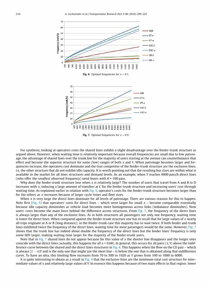
Fig. 6. Optimal frequencies for a ¼ 0:1.

Fig. 7. Optimal frequencies for a ¼ 0:9.

216 A. Gschwender et al. / Transportation Research Part A 88 (2016) 209–222

For synthesis, looking at operators costs the shared lines exhibit a slight disadvantage over the feeder-trunk structure asargued above. However, when waiting time is relatively important because overall frequencies are small due to low patron-age, the advantage of shared lines over the trunk line for the majority of users starting at the avenue can counterbalance thateffect and become the superior structure for some (low) ranges of both a and Y. When patronage becomes larger and fre-quencies increase, the operators cost dominate and the true competitor of the feeder-trunk structure are the exclusive lines,i.e. the other structure that do not exhibit idle capacity. It is worth pointing out that the resulting bus sizes are within what isavailable in the market for all lines structures and demand levels. As an example, when Y reaches 6000 pass/h direct lines(who offer the smallest observed frequency) need buses with K = 100 pass.

Why does the feeder-trunk structure lose when a is relatively large? The number of users that travel from A and B to Dincreases with a, inducing a large amount of transfers at C for the feeder-trunk structure and increasing users’ cost throughwaiting time. As explained earlier in relation with Fig. 5, operator’s costs for the feeder-trunk structure becomes larger thanfor the others as a increases because of larger cycle times and fleet sizes.

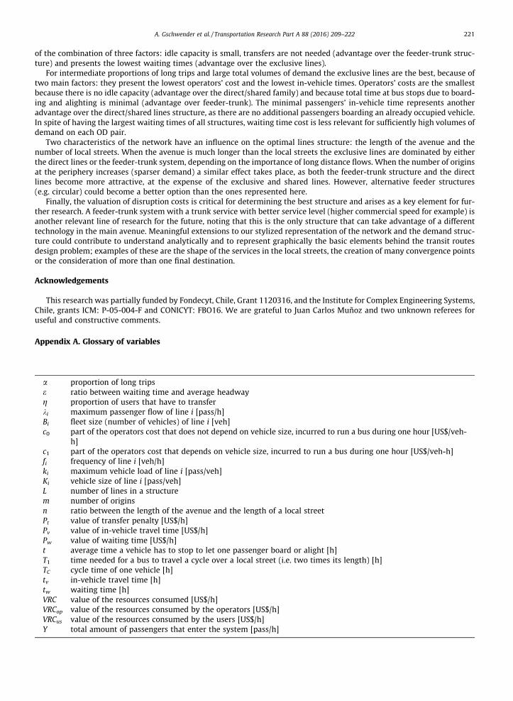
When a is very large the direct lines dominate for all levels of patronage. There are various reasons for this to happen.Note first (Fig. 5) that operators’ costs for direct lines – which were larger for small a – become comparable essentiallybecause idle capacity diminishes as vehicle load becomes more homogeneous across links (imbalance diminishes). Nowusers’ costs become the main force behind the difference across structures. From Fig. 7, the frequency of the direct linesis always larger than any of the exclusive lines. As in both structures all passengers see only one frequency, waiting timeis lower for direct lines. When compared against the feeder-trunk structure one has to recall that for large values of a nearlyall trips originate at A or B (long distance); in the feeder-trunk case this majority has to wait twice. If both feeder and trunklines exhibited twice the frequency of the direct lines, waiting time for most passengers would be the same. However, Fig. 7shows that the trunk line has indeed about double the frequency of the direct lines but the feeder lines’ frequency is onlysome 60% larger, making waiting time larger for the majority of the feeder-trunk users.

Note that in Fig. 7 shared lines do not appear because for this value of a the shorter line disappears and the longer onescoincide with the direct lines (actually, this happens for all a > 0.68). In general, this occurs for all pairs (a,Y) above the indif-ference curve between the shared and the direct lines structures in Fig. 4. This happens when the flow on the CD pair – whichis always (1 � a)Y and is the only one that might use the short line – is below the one that is obtained along that indifferencecurve. To have an idea, this limiting flow increases from 70 to 500 to 1920 as Y grows from 100 to 1000 to 6000.

It is quite interesting to obtain as a result in Fig. 4 that the exclusive lines are the minimum total cost structure for inter-mediate values of a and relatively large values of Y. In essence this happens because of two main effects in that region: lower

A. Gschwender et al. / Transportation Research Part A 88 (2016) 209–222 217

operators’ costs (as shown in Fig. 5) and lower in-vehicle time (as shown in Fig. 8). Regarding operators’ costs, exclusive linesdo not exhibit idle capacity and the absence of transfers favors lower cycle times and lower fleets. This same last fact causesshorter in-vehicle time for the users. It can be verified that for large values of Y and intermediate values of a the differencesin operators’ costs and in-vehicle times among structures dominate over the differences in waiting time; recall that for theexclusive lines structure waiting times on each OD pair depend only on the flow (that determines frequency) on that pair,served exclusively by one line, i.e. large values of patronage on each of the three OD pairs are needed.

Finally, Fig. 9 is quite helpful to highlight the large variation of waiting time as Y increases for all a values and all linesstructures, falling from a range 9–12 min to around 2 min as Y increase from 100 to 1900.

This confirms what was mentioned earlier regarding the relevance of waiting time when total patronage is relatively low.The advantage of the direct lines structure is evident for the users and could be counterbalanced by the larger operators costswhen a is small.

5. The impact of transfer penalties

The feeder-trunk structure is the only one that includes transfers. As in all passenger modes, moving from one vehicle toanother induces three effects on users: additional waiting time, additional walking time and disruption of the trip, i.e. abreaking in the process. Only the first effect has been included in the analysis in the previous section, making this the mostfavorable case for the feeder-trunk structure. Now we want to study the impact of including the other two effects. It isimportant to stress the fact that neither operators’ cost nor frequency, waiting and in-vehicle times at the optimum areaffected by the value of the transfer penalty; this makes their analysis in the base case also valid for the scenarios presentedin this section. That this is indeed the case can be seen from Eq. (1), where the term Ptg does not depend on frequency, theoptimization variable, and, therefore it vanishes when obtaining the first order conditions. Thus, the walking and disruptioncomponents of the transfer cost appears only as an additive term in the total cost of the feeder-trunk structure, potentiallyaffecting the optimal structures in the (a,Y) space. Let us examine how relevant this could be, which requires inputting val-ues for the so far omitted components.

There is no agreement on how important the disruption for a user is, i.e. the interruption of the trip by itself irrespectiveof the conditions (distance, slope, facilities) of the space between the alighting and boarding points (see Raveau et al., 2014)and of the additional waiting time. Although this is a research topic on its own, from the synthesis offered by Currie (2005)analyzing various cases (cities, trip purpose) and modes, disruption has been valued from 2 to 50 equivalent in-vehicleminutes (EIVM), a wide range indeed (5 to 50 if only bus trips are considered). Walking time induced by a transferdepends on the physical arrangement of facilities, starting from zero. To include these two dimensions in our analysis wewill consider two additional arbitrary scenarios: one with 12 EIVM of disruption only, a small amount, and anotherwith 22 EIVM (the average of Currie’s for bus) plus 4.5 walking minutes – a rather large transfer walk, equivalent to 13.5EIVM – for a total of 35.5 EIVM, a moderate-high value. Note that this makes Pt in problem (1) equal to the number of EIVMtimes Pv.

In Fig. 10 we show the optimal lines structure in the (a,Y) space for the base case and the two scenarios just described.The impact on the region where the feeder-trunk structure wins is apparent: the size of this region reduces dramatically infavor of the two immediate alternatives, i.e. the shared lines for low values of Y and the exclusive structure for large patron-age. Note that the value of a below which the feeder-trunk structure becomes interesting drops from 0.55 to 0.11 to 0.02when moving from the base case to scenarios 1 (low value for disruption) and 2 (mid value for disruption plus heavywalking) respectively. As a conclusion, when transfer costs are incorporated the feeder-trunk structure seems advantageousonly for very low values of a.

Fig. 8. In-vehicle time (min) for intermediate values of a.

Fig. 9. Waiting time (min) for intermediate values of a.

Fig. 10. Min cost structures for the three scenarios of transfer costs.

218 A. Gschwender et al. / Transportation Research Part A 88 (2016) 209–222

There are planning and design implications of these results that are quite relevant. First, walking time at a transfer point isindeed important and makes the physical arrangement of facilities a key design element, as the need to change level and theavailability of escalators or elevators (Raveau et al., 2014), and the configuration and capacity of the interchange. Second,even if walking time were nil (e.g. alighting and boarding at the same bus stop or platform) disruption would still be presentand assigning a value becomes an issue. Therefore, the study of the conditions behind the large dispersion of values is a rel-evant research task.

6. Sensitivity analysis of spatial parameters

6.1. Length of the avenue

So far we have considered that the distance between the collecting point C and the destination D – the avenue – is twicethe length of the local streets, i.e. n = 2. The analytical results in Section 3, however, were obtained as a function of n. To visu-alize the effect of nwe represent in Fig. 11 a case in which the length of the avenue is five times the length of the local streets.

The figure clearly shows that increasing the length of the avenue diminishes the region where the exclusive lines dom-inate. The FT system wins space for medium low values of awhile the direct lines win for medium high values. Each of thesecases can be intuitively explained with the help of Table 1, where one can see that the advantage of the FT system is repre-sented by the presence of economies of density along the avenue that now is much longer, while the disadvantage is thepresence of transfers; however, the effect of transfers on waiting, cycle and in-vehicle times does not depend on nwhile cycleand in-vehicle time do increase with n. The disadvantage, therefore, becomes less important. Regarding the direct lines, theironly disadvantage against the exclusive lines is the existence of idle capacity in the local streets, which looses importance asn grows. Note that the region where the shared lines dominate practically disappears; the direct lines structure is superior(see purple lines in Fig. 11).

Fig. 11. Effect of the length of the avenue.

A. Gschwender et al. / Transportation Research Part A 88 (2016) 209–222 219

As n increases the options tends to reduce to a choice between the direct and feeder-trunk structures. The former dom-inates for large values of awhile the latter dominates for low values, i.e. when the proportion of long distance users is small.The frontier between the regions where these two structures dominate, represented by the blue line in Fig. 11, does notchange much with n.

6.2. Dispersion of the population using feeder lines

Behind the distribution of total flow as represented in Fig. 1b there is an implicit representation of demand along localstreets AC and BC. What if demand was sparser? Demand dispersion is linked with the number of origins associated withlocal flows, and can be thought of as flows converging to different points along the avenue or as flows converging at C frommany different directions. In our model this could be represented as in Fig. 12, where the same aY – from the periphery to D –is distributed among m origins converging to neighbor points along the avenue, condensed at C such that m = 2 representsthe case analyzed in the previous sections. This could create a case more favorable to the feeder-trunk scheme because –recalling Fig. 2 – it is the structure that seems to adapt better to a situation where the long trips are originated at manypoints.

As seen in the previous section, there is a large dispersion of values that could be assigned to transfer disruption by itself;moreover, transfer walking time (distance and conditions) is very much case dependent. In order to examine dispersion atthe origins in a controlled way we will develop the analysis using the treatment of transfers of the base case, i.e. additionalwaiting time only. Indeed, this is the case most favorable to the feeder-trunk scheme.

Under this slightly modified setting, the four structures introduced in Fig. 2 can be generalized in a straightforward man-ner, with m local streets and the corresponding m origins similar to A or B. The results obtained in Section 3 could be gen-eralized to get the VRC for each case with analytical solution. These are shown in Eqs. (21), (22) and (23) for the closedsolutions. Note that for m = 2 Eqs. (11), (14) and (17) are recovered for DIR, FT and EXC respectively.

VRC�DIR ¼ 2tYc0 þ

ffiffiffiffiffiffiffiffiffiffiffiffiffiffiffiffiffiffiffiffiffiffiffiffiffiffiffiffiffiffiffiffiffiffiffiffiffiffiffiffiffiffiffiffiffiffiffiffiffiffiffiffiffiffiffiffiffiffiffiffiffiffiffiffiffiffiffiffiffiffiffiffiffiffiffiffiffiffiffiffiffiffiffiffiffiffiffiffiffiffiffiffiffiffiffiffiffiffiffiffiffiffiffiffiffiffiffiffiffiffiffiffiffiffiffiffiffiffiffiffiffiffiffiffiffiffiffiffiffiffiffiffiffiffiffiffiffiffi2ð1þ nÞT1Yc0ð4c1tY þ 2ð1þ am� aÞePw þ Pv tYð1� 2a2 þ 2aÞÞ

qþ T1Y c1ðnþ 1Þ þ Pv

2ðnþ aÞ

� �ð21Þ

VRC�FT ¼ 2tYc0ð1þ aÞ þ

ffiffiffiffiffiffiffiffiffiffiffiffiffiffiffiffiffiffiffiffiffiffiffiffiffiffiffiffiffiffiffiffiffiffiffiffiffiffiffiffiffiffiffiffiffiffiffiffiffiffiffiffiffiffiffiffiffiffiffiffiffiffiffiffiffiffiffiffiffiffiffiffiffiffiffiffi2YT1ac0ð4ac1tY þ 4emPw þ PvatYÞ

pþ

ffiffiffiffiffiffiffiffiffiffiffiffiffiffiffiffiffiffiffiffiffiffiffiffiffiffiffiffiffiffiffiffiffiffiffiffiffiffiffiffiffiffiffiffiffiffiffiffiffiffiffiffiffiffiffiffiffiffiffiffiffiffiffiffiffiffi2nT1Yc0ð4c1tY þ 2ePw þ Pv tYÞ

pþ T1Yðnþ aÞ c1 þ Pv

2

� �ð22Þ

VRC�EXC ¼ 2tYc0 þ

ffiffiffiffiffiffiffiffiffiffiffiffiffiffiffiffiffiffiffiffiffiffiffiffiffiffiffiffiffiffiffiffiffiffiffiffiffiffiffiffiffiffiffiffiffiffiffiffiffiffiffiffiffiffiffiffiffiffiffiffiffiffiffiffiffiffiffiffiffiffiffiffiffiffiffiffiffiffiffiffiffiffiffiffiffiffiffiffiffiffiffi2c0að1þ nÞT1Yð4ac1tY þ 2mePw þ aPv tYÞ

pþ

ffiffiffiffiffiffiffiffiffiffiffiffiffiffiffiffiffiffiffiffiffiffiffiffiffiffiffiffiffiffiffiffiffiffiffiffiffiffiffiffiffiffiffiffiffiffiffiffiffiffiffiffiffiffiffiffiffiffiffiffiffiffiffiffiffiffiffiffiffiffiffiffiffiffiffiffiffiffiffiffiffiffiffiffiffiffiffiffiffiffiffiffiffiffiffiffiffiffiffiffiffiffiffiffiffiffiffiffiffiffiffiffi2c0ð1� aÞnT1Yð4ð1� aÞc1tY þ 2ePw þ ð1� aÞPv tYÞ

pþ T1Yðaþ nÞ c1 þ Pv

2

� �ð23Þ

Fig. 13 shows the regions in the (a,Y) space where each structure is the best, for m = 1, 2 and 3. We do not use larger val-ues ofm, because in those cases there may be other lines structures that could be more adequate to serve the sparse demand(e.g. one or more circular feeder routes). It can be seen from Fig. 13 that, as expected, the region where the feeder-trunkstructure is the best grows with m. The region where the direct lines structure is the best also grows with m, whereasthe opposite occurs with the exclusive and shared lines.

Fig. 12. Representation of a sparse long distance demand.

Fig. 13. Effect of the number of local streets.

220 A. Gschwender et al. / Transportation Research Part A 88 (2016) 209–222

7. Conclusions

We analyze the best way, considering both users’ and operators’ costs, to serve a public transport network where severalflows converge into a main avenue. We find the best structure among four alternatives: feeder-trunk, direct, shared andexclusive lines, including the optimal frequencies and bus sizes.

Although the feeder-trunk structure never presents idle capacity (as direct and shared lines do), we have found that itdominates only for low proportions of long trips, because of three conditions that prevail under these circumstances:

– the feeder fleet can be better adjusted to the low demand in the periphery (smaller vehicles) reducing waiting times there(contrary to the exclusive lines structure which shows very large waiting times in the periphery);

– the advantages of economies of density in the avenue become relevant; and– the proportion of passengers that need to transfer is low.

However, the proportion of long trips below which the feeder-trunk structure dominates strongly diminishes when trans-fer disruption and additional walking time at transfer points are considered.

Therefore, in most cases some form of direct lines dominates: shared, pure direct or exclusive. For every value of the totaldemand there is a proportion of long trips beyond which the optimal frequency of the short line in the shared lines structuredrops to zero and this structure collapses into the direct lines; when this short line exists, the shared lines structure is betterthan the direct lines structure. For high proportions of long trips the direct/shared lines structure family dominates because

A. Gschwender et al. / Transportation Research Part A 88 (2016) 209–222 221

of the combination of three factors: idle capacity is small, transfers are not needed (advantage over the feeder-trunk struc-ture) and presents the lowest waiting times (advantage over the exclusive lines).

For intermediate proportions of long trips and large total volumes of demand the exclusive lines are the best, because oftwo main factors: they present the lowest operators’ cost and the lowest in-vehicle times. Operators’ costs are the smallestbecause there is no idle capacity (advantage over the direct/shared family) and because total time at bus stops due to board-ing and alighting is minimal (advantage over feeder-trunk). The minimal passengers’ in-vehicle time represents anotheradvantage over the direct/shared lines structure, as there are no additional passengers boarding an already occupied vehicle.In spite of having the largest waiting times of all structures, waiting time cost is less relevant for sufficiently high volumes ofdemand on each OD pair.

Two characteristics of the network have an influence on the optimal lines structure: the length of the avenue and thenumber of local streets. When the avenue is much longer than the local streets the exclusive lines are dominated by eitherthe direct lines or the feeder-trunk system, depending on the importance of long distance flows. When the number of originsat the periphery increases (sparser demand) a similar effect takes place, as both the feeder-trunk structure and the directlines become more attractive, at the expense of the exclusive and shared lines. However, alternative feeder structures(e.g. circular) could become a better option than the ones represented here.

Finally, the valuation of disruption costs is critical for determining the best structure and arises as a key element for fur-ther research. A feeder-trunk system with a trunk service with better service level (higher commercial speed for example) isanother relevant line of research for the future, noting that this is the only structure that can take advantage of a differenttechnology in the main avenue. Meaningful extensions to our stylized representation of the network and the demand struc-ture could contribute to understand analytically and to represent graphically the basic elements behind the transit routesdesign problem; examples of these are the shape of the services in the local streets, the creation of many convergence pointsor the consideration of more than one final destination.

Acknowledgements

This research was partially funded by Fondecyt, Chile, Grant 1120316, and the Institute for Complex Engineering Systems,Chile, grants ICM: P-05-004-F and CONICYT: FBO16. We are grateful to Juan Carlos Muñoz and two unknown referees foruseful and constructive comments.

Appendix A. Glossary of variables

a

proportion of long trips e ratio between waiting time and average headway g proportion of users that have to transfer ki maximum passenger flow of line i [pass/h] Bi fleet size (number of vehicles) of line i [veh] c0 part of the operators cost that does not depend on vehicle size, incurred to run a bus during one hour [US$/veh-

h]

c1 part of the operators cost that depends on vehicle size, incurred to run a bus during one hour [US$/veh-h] fi frequency of line i [veh/h] ki maximum vehicle load of line i [pass/veh] Ki vehicle size of line i [pass/veh] L number of lines in a structure m number of origins n ratio between the length of the avenue and the length of a local street Pt value of transfer penalty [US$/h] Pv value of in-vehicle travel time [US$/h] Pw value of waiting time [US$/h] t average time a vehicle has to stop to let one passenger board or alight [h] T1 time needed for a bus to travel a cycle over a local street (i.e. two times its length) [h] TC cycle time of one vehicle [h] tv in-vehicle travel time [h] tw waiting time [h] VRC value of the resources consumed [US$/h] VRCop value of the resources consumed by the operators [US$/h] VRCus value of the resources consumed by the users [US$/h] Y total amount of passengers that enter the system [pass/h]

222 A. Gschwender et al. / Transportation Research Part A 88 (2016) 209–222

References

Aldaihani, M.M., Quadrifoglio, L., Dessouky, M.M., Hall, R., 2004. Network design for a grid hybrid transit service. Transp. Res. Part A 38, 511–530.Badia, H., Estrada, M., Robusté, F., 2014. Competitive transit network design in cities with radial street patterns. Transp. Res. Part B 59, 161–181.Brueckner, J.K., 2004. Network structure and airline scheduling. J. Ind. Econ. 52, 219–312.Ceder, A., 2001. Operational objective functions in designing public transport routes. J. Adv. Transp. 35, 125–144.Chang, S.K., Schonfeld, P.M., 1991. Multiple period optimization of bus transit systems. Transp. Res. Part B 25, 453–478.Currie, G., 2005. The demand performance of bus rapid transit. J. Public Transp. 8, 41–55.Daganzo, C.F., 2010. Structure of competitive transit networks. Transp. Res. Part B 44, 434–446.Díaz, G., Gómez-Lobo, A., Velasco, A., 2002. Micros en Santiago: hacia la licitación del 2003 (Buses in Santiago: Towards the 2003 Tendering Process).

Seminario ‘‘El Chile que Viene I”. Expansiva, Centro de Estudios Públicos, Santiago.El-Hifnawi, M.B., 2002. Cross-town bus routes as a solution for decentralized travel: cost-benefit analysis for Monterrey, Mexico. Transp. Res. Part A 36,

127–144.Estrada, M., Roca-Riu, M., Badia, H., Robusté, F., Daganzo, C.F., 2011. Design and implementation of efficient transit network: procedure, case study and

validity test. Transp. Res. Part A 45, 935–950.Jansson, J.O., 1980. A simple bus line model for optimisation of service frequency and bus size. J. Transp. Econ. Policy 14, 53–80.Jansson, J.O., 1984. Transport System Optimization and Pricing. John Wiley & Sons, Chichester.Jara-Díaz, S., Gschwender, A., Ortega, M., 2012. Is public transport based on transfers optimal? A theoretical investigation. Transp. Res. Part B 46, 808–816.Jara-Díaz, S., Gschwender, A., Ortega, M., 2014. The impact of a financial constraint on the spatial structure of public transport services. Transportation 41,

21–36.Kepaptsoglou, K., Karlaftis, M., 2009. Transit routes networks design problem: review. J. Transp. Eng. 135, 491–505.Kocur, G., Hendrickson, C., 1982. Design of local bus service with demand equilibration. Transp. Sci. 16, 149–170.Mohring, H., 1972. Optimization and scale economies in urban bus transportation. Am. Econ. Rev. 62, 591–604.Quadrifoglio, L., Li, X., 2011. A methodology to derive the critical demand density for designing and operating feeder transit services. Transp. Res. Part B 43,

922–935.Raveau, S., Guo, Z., Muñoz, J.C., Wilson, N., 2014. A behavioural comparison of route choice on metro networks: time, transfers, crowding, topology and

socio-demographics. Transp. Res. Part A 66, 185–195.Sandoval, E., 2010. Recuperando la flexibilidad de los BRT: de Transmilenio a Guangzhou, Cúcuta y Buenos Aires. Actas del XVI Congreso Latinoamericano de

Transporte Público y Urbano. 6–8 Octubre 2010, Ciudad de México.Tirachini, A., Hensher, D., Jara-Díaz, S., 2010. Comparing operator and users costs of light rail, heavy rail and bus rapid transit over a radial public transport

network. Res. Transp. Econ. 29, 231–242.