Transportation Research Part A 70 (2014) 194–209

Contents lists available at ScienceDirect

Transportation Research Part A

journal homepage: www.elsevier .com/locate / t ra

Consumers’ willingness to pay for alternative fuel vehicles: Acomparative discrete choice analysis between the US and Japan

http://dx.doi.org/10.1016/j.tra.2014.10.0190965-8564/� 2014 Elsevier Ltd. All rights reserved.

⇑ Corresponding author at: 7-22-1 Roppongi, Minato-ku, Tokyo 106-8677, Japan. Tel.: +81 3 6439 6000.E-mail address: mtanaka@grips.ac.jp (M. Tanaka).

1 See his ‘‘Presidential Memorandum—Federal Fleet Performance’’ dated May 24, 2011 available at http://www.whitehouse.gov/the-press-office/201presidential-memorandum-federal-fleet-performance.

2 Sixteen models are listed as eligible for the federal tax credit on the government website http://www.fueleconomy.gov/feg/taxevb.shtml. The salefor electric vehicles are from the Electric Drive Transportation Association at http://www.electricdrive.org/index.php?ht=d/sp/i/20952/pid/20952.

3 See pp. 7 and 25 of The Motor Industry of Japan (2012). In calendar year 2010 there were 4,212,267 new passenger vehicle registrations, and 3,522011.

Makoto Tanaka a,⇑, Takanori Ida b, Kayo Murakami b, Lee Friedman c

a National Graduate Institute for Policy Studies, Japanb Kyoto University, Japanc University of California Berkeley, USA

a r t i c l e i n f o

Article history:Received 21 September 2013Received in revised form 12 September 2014Accepted 16 October 2014

Keywords:Willingness to payStated preferenceDiscrete choiceElectric vehicle (EV)Plug-in hybrid electric vehicle (PHEV)

a b s t r a c t

This paper conducts a comparative discrete choice analysis to estimate consumers’ willing-ness to pay (WTP) for electric vehicles (EVs) and plug-in hybrid electric vehicles (PHEVs) onthe basis of the same stated preference survey carried out in the US and Japan in 2012. Wealso carry out a comparative analysis across four US states. We find that on average US con-sumers are more sensitive to fuel cost reductions and alternative fuel station availabilitythan are Japanese consumers. With regard to the comparative analysis across the fourUS states, consumers’ WTP for a fuel cost reduction in California is considerably greaterthan in the other three states. We use the estimates obtained in the discrete choice analysisto examine the EV/PHEV market shares under several scenarios. In a base case scenariowith relatively realistic attribute levels, conventional gasoline vehicles still dominate bothin the US and Japan. However, in an innovation scenario with a significant purchase pricereduction, we observe a high penetration of alternative fuel vehicles both in the US andJapan. We illustrate the potential use of a discrete choice analysis for forward-looking pol-icy analysis, with the future opportunity to compare its predictions against actual revealedchoices. In this case, increased purchase price subsidies are likely to have a significantimpact on the market shares of alternative fuel vehicles.

� 2014 Elsevier Ltd. All rights reserved.

1. Introduction

President Barack Obama has called for 1 million alternative fuel vehicles to be on the road in the US by 2015.1 Automobilemanufacturers have just begun to make such vehicles available in the US marketplace, with approximately sixteen differentmodels available at the time of this writing and total sales from 2011 through September 2012 just over 40,000 units.2 Similarly,Japan’s Ministry of Economy has set a goal of having 20% of new car sales be such vehicles by 2020, although sales at this timeremain quite modest: for fiscal year 2010, 4816 electric vehicles or just over 1% were provided to the domestic market.3 Clearly

1/05/24/

s figures

4,788 in

M. Tanaka et al. / Transportation Research Part A 70 (2014) 194–209 195

there is a long way to go to reach these goals. The current vehicles are largely either electric (EV) or plug-in hybrid electric(PHEV), although other alternative fuels such as hydrogen or natural-gas powered vehicles could become more significant inthe future.4 Particularly, PHEVs have recently received considerable attention in the transportation literature (Musti andKockelman, 2011; Graham-Rowe et al., 2012; Krupa et al., 2014). The US, Japan, and other countries are using and consideringvarious public policies to help achieve these goals for cleaner vehicles.

In recent years, Japan has provided a variety of incentives to purchase green vehicles, including exemptions from itsacquisition tax at purchase and some reductions in its tonnage tax, both totaling about 5.7% of the purchase price.5 In theUS, there is currently a federal tax credit of up to $7500 for the purchase of qualifying vehicles, and the President has announcedthat he would like to expand this credit to $10,000. What effect is a policy change like this likely to have? The analysis presentedin this paper suggests that, other things being equal, such an increase is likely to have a significant impact. Of course, otherthings may not be equal. For example, some US states like California have additional tax credits that could be raised or loweredover time. The California Clean Vehicle Rebate Project currently provides a rebate of up to $2500 per vehicle (Center forSustainable Energy, 2013), but it is not clear for how long such incentives will continue. Thus our analysis is not a forecast,but an investigation of the extent that different purchase factors matter to consumers.

Given the early stage of development for alternative fuel vehicles, empirical revealed preference data from actual pur-chases have not been sufficiently accumulated. Therefore, we adopt a stated preference (SP) method. SP data come from sur-vey responses to hypothetical choices, and take into account certain types of market constraints useful for forecastingchanges in consumer behaviors. The responses may be affected by the degree of contextual realism as perceived by the sur-vey respondents.

Most studies on the demand for clean-fuel vehicles have used the SP method. Past studies on clean-fuel or electric vehi-cles are summarized in Table 1. Early studies on clean-fuel vehicles include those of Beggs et al. (1981) and Calfee (1985) inresponse to the oil crisis of the 1970s. The zero-emission vehicle mandate in California also stimulated a series of studies onEVs. Studies on the potential demand for EVs in California include Bunch et al. (1993), Segal (1995), Brownstone and Train(1999), Brownstone et al. (2000), and Hess et al. (2012). Many demand studies for clean-fuel vehicles focus on an individualcountry: the US (Hidrue et al., 2011), Canada (Ewing and Sarigöllü, 2000; Potoglou and Kanaroglou, 2007; Mau et al., 2008),Germany (Ziegler, 2012; Achtnicht et al., 2012; Hackbarth and Madlener, 2013), Norway (Dagsvik et al., 2002), Japan (Itoet al., 2013), South Korea (Ahn et al., 2008), and China (Qian and Soopramanien, 2011). Very few studies conduct a compar-ative discrete choice analysis across multiple countries. One exception is Axsen et al. (2009), which investigates SP data inthe US and Canada. However, to the best of our knowledge, no comparative discrete choice analysis on the demand for clean-fuel vehicles between the US and Japan has been conducted.6

This paper contributes to the existing literature in three ways. First, we conduct a comparative discrete choice analysis onalternative fuel vehicles between the US and Japan based on the same online stated preference survey with a large sample inboth countries. Second, we also carry out a discrete choice analysis across the four US states (California, Texas, Michigan, andNew York) for a state comparison. Third, our analysis is policy-relevant in the sense that we account for EVs, PHEVs, andconventional gasoline vehicles to represent consumer choice among conventional and new technologies, and to simulatehow these choices may be affected by public policies in the context of the US and Japan.7

Our main findings are as follows. Regarding the comparison between the US and Japan, we find that US consumers aremore sensitive to fuel cost reductions and to alternative fuel station availability than are Japanese consumers, while consum-ers in both countries are equally sensitive to the driving range on a full battery and to emissions reduction. With regard tocomparative analysis across the four US states, we find that consumers’ willingness to pay (WTP) for a fuel cost reduction inCalifornia is considerably greater than in the other three states. The WTP values for other attributes are very similar acrossthose states except for Michigan. We then conduct a numerical evaluation of EV/PHEV market shares based on the estimatesobtained in the discrete choice analysis. In a base case scenario with relatively realistic attribute levels, conventional gasolinevehicles still dominate both in the US and Japan. However, in an innovation scenario with a significant purchase price reduc-tion, we observe a high penetration of alternative fuel vehicles both in the US and Japan.

The remainder of this paper is organized as follows. Section 2 explains the online stated preference survey method andthe experimental design. Section 3 describes the discrete choice model used for estimation. Section 4 reports the estimationresults and measures the WTP values of the attributes. Section 5 presents the diffusion analysis and its implications for thefuture spread of alternative fuel vehicles. Section 6 presents a brief illustration of the potential of discrete choice analysis as atool for forward-looking policy analysis. Finally, Section 7 concludes the paper.

4 An EV uses one or more electric motors with batteries for propulsion, while a PHEV combines an internal combustion engine and electric motors withbatteries that can be recharged via an external electric power source at home or at a public charging station.

5 See p. 45 of The Motor Industry of Japan (2012).6 Karplus et al. (2010) used a computable general equilibrium (CGE) model to investigate the prospects for PHEV market entry in the US and Japan,

particularly focusing on the production structure of the PHEV sector with cost share parameters. They, however, did not use SP data/discrete choice analysis onthe demand for clean-fuel vehicles.

7 Our work is in line with other studies that use a discrete choice analysis for forward-looking policy discussions (e.g., Ewing and Sarigöllü, 1998; Horne et al.,2005; Daziano and Bolduc, 2013).

Table 1Summary of past SP studies on clean fuel or electric vehicles (an extension of the summary in Horne et al., 2005 and Hidrue et al., 2011).

Study Econometricmodel

Numberofattributes,and levels

List of attributes used

Purchaseprice

Operatingcost

Drivingrange

Emissionsdata

Fuelavailability

Fueltype

Performance Vehicletype

Otherincentives

Beggs et al. (1981) Ranked logit 8, NA Price Fuel cost Range – – – Top speed,acceleration

Number ofseats, airconditioning

Warranty

Calfee (1985) Disaggregatemultinomial logit

5, NA Price Operating cost Range – – – Top speed Number ofseats

–

Bunch et al. (1993) Multinomial logit andnested logit

7, 4 Purchaseprice

Fuel cost Range Emissions level Fuel availability fueltype

Acceleration – –

Segal (1995) First choice model 7, 2–3 Price Fuel cost Range, refuelingduration

– Refueling location,refueling time ofday

Fueltype

– – –

Brownstone and Train(1999)1; Brownstoneet al. (2000)1

Multinomial logit andmixed logit; joint SP/RPMIXED LOGIT

13, 4 Price Home refuelingcost, service stationrefueling cost

Range Emissionreduction

Fuel availability,home refuelingtime

– Top speed,acceleration

Vehicle size,body type,luggage space

–

Ewing and Sarigollu (2000) Multinomial logit 7,3 Price Fuel cost, repair andmaintenance cost

Range – Charging time – Acceleration Commutingtime

–

Dagsvik et al. (2002) Ranked logit 4, NA Price Fuel cost Range – – – Top speed – –Potoglou and Kanaroglou

(2007)Nested logit 7, 4 Price Fuel cost,

maintenance cost– Emission

reductionFuel availability – Acceleration – Incentives

Horne et al. (2005)2 Multinomial logit 6, 2–5 Purchaseprice

Fuel cost – Emissionscompared tocurrent vehicle

Stations withproper fuel

– Powercompared tocurrentvehicle

Express laneaccess

–

Ahn et al. (2008) Multiple discrete-continuous extremevalue

6, 2–5 – Fuel price,maintenance cost

Fuel efficiency Enginedisplacement

– Fueltype

– Body type –

Mau et al. (2008) Multinomial logit 6, 3 Price Fuel cost Range – Fuel availability – – – Subsidy,warranty

Axsen et al. (2009) Multinomial logit; jointSP/RP multinomial logit

5, 3 Price Fuel price Fuel efficiency – – – Horsepower – Subsidy

Hidrue et al. (2011) Latent class 6, 4 price Fuel cost Range Emissionreduction

Charging time – Acceleration – –

Qian and Soopramanien(2011)

Multinomial logit andnested logit

6, 3 Price Fuel cost Range – Fuel availability Fueltype

– – Policyincentives

Ziegler (2012) Multinomial probit 5, 3 Price Fuel cost – Emissions Fuel availability – Horsepower – –Achtnicht et al. (2012) Logit 6, 7 Price Fuel cost – Emissions fuel availability Fuel

typeHorsepower – –

Hess et al. (2012) Mixed multinomiallogit, nested, cross-nested logit

12, 2–15 Purchaseprice

Fuel cost per year,maintenance costper year

Driving range,miles per gallonequivalent

– Fuel availability,refueling time

Fueltype

Acceleration Vehicle type,age of vehicle

Incentive

Ito et al. (2013) Multinomial logit andnested logit

9, 4 Price Fuel cost Range Emissionreduction

Fuel availability,refueling time

Fueltype

Acceleration body type,Manufacturer

–

Hackbarth and Madlener(2013)

Mixed logit 8, 3 Price Fuel cost Range Emissionreduction

Fuel availability,refueling time,charging time

– – – Policyincentives

This study Mixed logit 6, 2–4 Purchaseprice

Fuel cost Driving range Emissionreduction

FUEL availability,home plug–inconstruction

– – – –

1 The two papers used the same data.2 They conducted the survey within the context of vehicle type and commuting mode decisions. We extract the former part.

196M

.Tanakaet

al./TransportationR

esearchPart

A70

(2014)194–

209

M. Tanaka et al. / Transportation Research Part A 70 (2014) 194–209 197

2. Survey and design

This section explains the stated preference survey method and the experimental design. The survey was conducted onlinein February 2012 by consumer research companies both in the US and Japan that employ random sampling techniques toensure representative populations. We surveyed random samples of 4202 and 4000 consumers in four US states and Japan,respectively. Specifically, we focused on California (West), Texas (South), Michigan (Midwest), and New York (Northeast) asstates from four different regions in the US, with a sample size of just over 1000 from each state. These states were chosenbecause they represent different regions, but also because they each have different electricity systems overseen by state reg-ulators and differing clean vehicle policies.8 While we present our findings separately for each state, we also average theresponses across the four-state US sample to compare them with the Japanese responses. It should be understood that thisfour-state average is not intended to be statistically representative of the full US.9 In the case of Japan, which is under one reg-ulatory system, our sample of 4000 consumers covers all prefectures so as to represent an average Japanese population.10 Thesamples were randomly selected by the consumer research companies to ensure that the actual population distribution, agedistribution, and gender distribution were properly reflected.

Our survey focuses on consumer preferences for particular attributes of vehicles that affect their purchase decisions. Inthe marketing literature, using this type of survey to model consumer choice is often referred to as a conjoint analysis. Ifan excessive number of attributes and levels are included, respondents find it difficult to answer the questions. On the otherhand, if too few are included, the description of the alternatives becomes inadequate. Since the number of attributesbecomes unwieldy if we consider all possible combinations, we adopted an orthogonal planning method to avoid this problem(see Louviere et al., 2000, Ch. 4, for details).

There are pros and cons for a consumer considering purchasing an EV or PHEV. Driving an EV or PHEV can significantlyreduce expenses on gasoline or other fuels, and pollution is much lower than from conventional gasoline vehicles. On theother hand, the purchase prices of these vehicles are relatively high when compared to standard gasoline vehicles (at pres-ent, an additional $10,000 or more). Furthermore, the driving range on a full battery is still very limited, and finding a charg-ing station can be time consuming. Given these facts, we focus on the following six key attributes in this study: (1) purchaseprice premium, (2) fuel cost reduction (percentage) as compared with gasoline vehicles, (3) driving range on full battery, (4)emissions reduction (percentage) compared with gasoline vehicles, (5) alternative fuel station availability (expressed as apercentage of existing gas stations), and (6) home plug-in construction fee. Note that the driving range on a full battery isconcerned with consumer preference for the physical attribute of the EV/PHEV battery (‘‘range anxiety’’) rather than imply-ing a preference for fuel efficiency. After conducting several pretests, we determined the attribute levels of the EV/PHEV con-joint analysis as summarized in Table 2. We did not consider other attributes such as fuel type, performance, vehicle type,and other policy incentives as shown in Table 1. That is, the survey holds constant other attributes by providing a simpledescription of a hypothetical vehicle that does not vary apart from the six studied attributes.

Fig. 1 displays an example of one of the questions used on the EV/PHEV conjoint questionnaire. There are three alterna-tives: Alternative 1 denotes EV; Alternative 2 denotes PHEV; and Alternative 3 refers to gasoline vehicle purchases. There aresixteen questions in total that look like Fig. 1 except with different attributes. In addition, they are divided into two versionsof eight questions each by using a blocking methodology. All respondents are asked one of the two versions at random.

3. Model specification

This section describes the estimation model. Conditional logit (CL) models, which assume independent and identical dis-tribution (IID) of random terms, have been widely used in past studies. However, the property of independence from theirrelevant alternatives (IIA) derived from the IID assumption of the CL model is too strict to allow flexible substitution pat-terns. A nested logit (NL) model partially relaxes the strong IID assumptions by partitioning the choice set and allowingnested alternatives to have common unobserved components compared with non-nested alternatives. However, the NLmodel is not suited for our analysis because it cannot deal with the distribution of parameters at the individual level(Ben-Akiva and Bolduc, 2001). The best model for this study is an error component multinomial logit (ECML) model, whichaccommodates differences in the variance of error components for each alternative. This model is flexible enough to over-

8 Michigan, the historic home state of the US motor vehicle industry, is also a state in which electricity service is provided largely by vertically-integratedutilities subject to rate-of-return regulation. Texas is a state with substantial retail and wholesale electricity competition, and the competitive retailers maymarket to induce customers to purchase plug-in electric vehicles. New York has wholesale competition and some retail competition (although not as much asTexas). California has significant wholesale competition, but not retail competition. In terms of clean vehicle policies, California adopted in 2004 emissionstandards that commit to a 30% reduction in GHG emissions by 2016, and it offers rebates of up to $2500 per vehicle for the purchase of qualifying alternativefuel vehicles. New York adopted the California emission standards in 2005, but does not offer financial incentives for the purchase of clean vehicles. Michiganand Texas do not have state emission standards or financial incentives.

9 These four states contain approximately 30% of the US population. To the extent that higher electricity prices discourage interest in alternative fuel vehicles,our sample may slightly understate the overall interest of the US population. While the average residential electricity bill in the four states ($105.26) is close tothe US average ($110.55), the average retail rate of $.144 per kWh in the four states is higher than the US average of $.115 and the average monthlyconsumption amount (763 kWh) is lower than in the US as a whole (858 kWh). These figures are from the US Energy Information Administration 2010 report onelectricity sales and revenue.

10 Japan is a more compact and homogeneous country, approximately equivalent in area to California but with a population of 128 million.

Table 2Attribute levels of conjoint analysis.

EV (Electric vehicle) PHEV (Hybrid electric vehicle with a plug-in function) Gasoline Vehicles

Level 1 Level 2 Level 3 Level 4 Level 1 Level 2 Level 3 Level 4 Level 1 Level 2 Level 3 Level 4

Purchase price/pricepremium

$1,000higher

$3,000higher

$5,000higher

$10,000higher

$1,000higher

$3,000higher

$5,000higher

$10,000higher

about $20,000 (fixed)

Fuel cost (compared withconventional gasolinevehicles)

60% off 80% off 40% off 60% off 0% off (asconventional)

10% off 20% off 30% off

Driving range 100 miles 200 miles 300 miles 400 miles 700 miles 800 miles 900 miles 1000 miles 400 miles 500 miles 600 miles 700 milesEmission reduction

(compared withconventionalgasoline vehicles)

70%reduction

80%reduction

90%reduction

100%reduction

50%reduction

60%reduction

70%reduction

80%reduction

No reduction 10%reduction

20%reduction

30%reduction

Alternative fuel availability(% of existing gasstations)

10% 30% 50% 70% 10% 30% 50% 70% –

Home plug-in constructionfee

No fee 1,000 US$ No fee 1,000 US$ –

Note: Among the respondents including those who are interested in alternative fuel vehicles, approximately 75% of the US respondents and 85% of Japanese respondents are thinking of ‘‘under $30,000’’ forpurchasing a future vehicle as shown in Table 3. Therefore, we assume the conventional purchase price for a gasoline vehicle at $20,000 in the choice experiment for simplification. This simplification may inducebias in estimation and a limit on this analysis, but can decrease the cognitive burden of the respondents in the survey task.

198M

.Tanakaet

al./TransportationR

esearchPart

A70

(2014)194–

209

Fig. 1. Example of conjoint questionnaire.

M. Tanaka et al. / Transportation Research Part A 70 (2014) 194–209 199

come the limitations of CL models by allowing for random taste variation, unrestricted substitution patterns, and the corre-lation of random terms over time (McFadden and Train, 2000). In the ECML model, alternative specific random individualeffects account for unobserved variations that are not accounted for by the other model components.

Assuming that parameter bn is distributed with density function f(bn) (Train, 2003; Louviere et al., 2000), the ECML spec-ification allows for repeated choices by each sampled decision maker in such a way that the coefficients vary across peoplebut are constant over each person’s choice situation. The logit probability of decision maker n choosing alternative i in choicesituation t is expressed as

11 Louup to 10Halton

12 81%genderin geogpreferen

LnitðbnÞ ¼YT

t¼1

expðVnitðbnÞÞXJ

j¼1

expðVnjtðbnÞÞ, #"

; ð1Þ

which is the product of normal logit formulas, given parameter bn, the observable portion of utility function Vnit, and alter-natives j = 1, . . . , J in choice situations t = 1, . . ., T. Therefore, the ECML choice probability is a weighted average of the logitprobability Lnit(bn) evaluated at parameter bn with density function f(bn), which can be written as

Pnit ¼Z

LnitðbnÞf ðbnÞdbn: ð2Þ

Accordingly, we can demonstrate variety in the parameters at the individual level using the maximum simulated likeli-hood (MSL) method for estimation with a set of 100 Halton draws.11 Furthermore, since each respondent completes eightquestions in the conjoint analysis, the data form a panel to which we can apply a standard random effect estimation.

In the linear-in-parameter form, the utility function can be written as

Unit ¼ a0xnit þ b0nznit þ enit; ð3Þ

where xnit denotes an observable variable, znit is an alternative error component, a denotes a fixed parameter vector, bn

denotes a random parameter vector, and enit denotes an independently and identically distributed extreme value (IIDEV)term. Here, for simplicity, we assume that the only random parameters included are the error components for each alterna-tive. Further, we set the utility of the no-choice alternative to be normalized to zero (baseline) and the error componentterms—as well as alternative specific constant terms—are added to all alternatives, including the no choice (baseline) alter-native. Since the ECML choice probability is not expressed in a closed form, simulations must be performed for the ECMLmodel estimation (see Train, 2003, for details).

4. Data description and estimation results

After briefly describing the data used in this study, we show the EV and PHEV estimation results in this section. First,Table 3 summarizes the basic demographic characteristics of the respondents in the four-state US and Japan samples.12

Table 3 also shows the preferences for EV/PHEV utilization. As shown, 57% and 41% of the respondents in the US and Japan sam-ples, respectively, indicate an intention to purchase a car within the next five years. Moreover, 60% and 53% of the respondentsin the US and Japan, respectively, show an interest in alternative fuel vehicles.

viere et al. (2000, p. 201) suggest that 100 replications are normally sufficient for a typical problem involving five alternatives, 1000 observations, andattributes (also see Revelt and Train, 1998). The adoption of the Halton sequence draw is an important issue (Halton, 1960). Bhat (2001) found that 100

sequence draws are more efficient than 1000 random draws for simulating an ECML model.and 72% of the respondents replied that they are the primary handlers of household bills in the US and Japan, respectively. Some of the asymmetric

distribution between the US and Japan in this survey might be attributed to some extent to who primarily handles household bills. While our interest israphic differences, an alternative modeling approach would be to explore the extent to which demographic differences can explain the statedces. We explore such an approach briefly in Appendix.

Table 3Respondents’ characteristics

US respondents(%)

California(%)

Texas(%)

Michigan(%)

New York(%)

Japaneserespondents (%)

Gender (Male) 38.2 44.6 37.4 32.8 38.2 56.0Age from 30’s to 50’s 58.3 60.2 55.2 61.8 56.0 77.9Married/couple 69.8 64.3 72.3 73.5 68.9 80.3Detached house dwelling 72.0 62.0 78.1 78.8 68.4 54.7Annual household income between $30,000 to

$70,00041.9 35.6 44.4 47.6 39.8 50.7

Ownership of conventional gasoline vehicles 96.0 96.0 97.0 96.4 94.4 78.5Intent to purchase a car within next five years 56.7 58.8 56.2 54.9 52.5 41.3

Type of car respondents are planning to purchaseFour-door sedan 43.5 50.6 37.3 35.5 51.0 20.9Two-door sedan 5.0 8.0 5.2 3.7 3.1 0.6Station wagon 1.4 1.0 1.3 1.7 1.6 11.7Sports utility vehicle (US only) 27.8 18.6 32.8 31.4 28.3 –Mini-vehicle (Keicar) (Japan only) – – – – – 22.5Compact car 6.1 6.3 6.4 7.5 4.2 21.1Minivan 5.1 2.8 3.1 9.4 5.1 18.5Sports car 3.8 5.3 3.9 2.8 3.0 1.6Others 7.3 7.3 10.0 8.0 3.7 3.2

Price range for purchasing a next vehicleUnder $20,000 32.2 28.5 31.0 39.0 30.4 54.7Between $20,000 to $30,000 42.4 41.4 45.4 41.5 41.3 29.5Between $30,000 to $40,000 18.1 20.0 16.5 16.4 19.6 9.7Between $40,000 to $50,000 5.1 6.2 5.6 2.7 5.9 3.3Over $50,000 2.2 4.0 1.5 0.5 2.8 2.7

Interest in alternative fuel vehicles (very/moderatelyinterested)

59.5 67.2 55.6 56.6 58.8 52.8

Interest in charging alternative fuel vehicle at home 82.3 78.8 84.5 86.7 78.7 70.3

200 M. Tanaka et al. / Transportation Research Part A 70 (2014) 194–209

We now discuss the EV and PHEV estimation results for the US and Japan. We also present the results for the four USstates separately. Table 4 shows the estimation results for the combined four-state US sample and for Japan. The McFaddenR2 values are 0.3378 for the former and 0.4223 for the latter, both of which are sufficiently high for a discrete choice model.We assume that alternative specific parameters (error components) are distributed normally, and the mean and standarddeviation values are reported.

All the estimates (means) are statistically significant at the 1% level. For both the US and Japan, the signs of the estimatesare positive for reduction in fuel costs, driving range, emissions reduction, and alternative fuel station availability, and neg-

Table 4Estimation results for US and Japan.

US respondents Japanese respondents

Coeff. Std. Err. WTP (US$) Coeff. Std. Err. WTP (US$)

<non random parameters>ASC for EV 5.77049 0.16766⁄⁄⁄ – 7.94481 0.19466⁄⁄⁄ –ASC for PHEV 6.91993 0.16739⁄⁄⁄ – 9.25162 0.19855⁄⁄⁄ –ASC for gasoline vehicles 6.57852 0.11927⁄⁄⁄ – 7.44048 0.13909⁄⁄⁄ –Purchase price (US$) �0.00030 0.00000⁄⁄⁄ – –0.00036 0.00000⁄⁄⁄ –Fuel cost (% off compared with gasoline vehicles) 0.01485 0.00099⁄⁄⁄ 49.84 0.01315 0.00112⁄⁄⁄ 36.74Range (miles) 0.00064 0.00008⁄⁄⁄ 2.15 0.00077 0.00005⁄⁄⁄ 2.15Emission reduction (% reduction compared with gasoline vehicles) 0.00864 0.00092⁄⁄⁄ 29.00 0.00936 0.00101⁄⁄⁄ 26.15

Alternative fuel station availability(% of existing gas stations) 0.01485 0.00050⁄⁄⁄ 49.84 0.01202 0.00059⁄⁄⁄ 33.59Home plug-in construction fee (US$100) �0.06359 0.00199⁄⁄⁄ �213.41 �0.06052 0.00232⁄⁄⁄ �169.10

<Standard deviation of error components>EV 1.58005 0.0354⁄⁄⁄ – 1.92815 0.0507⁄⁄⁄ –PHEV 0.10192 0.0633 – 1.13103 0.0640⁄⁄⁄ –Gasoline vehicles 3.85320 0.0792⁄⁄⁄ – 4.97706 0.1089⁄⁄⁄ –Not buy 3.59628 0.0663⁄⁄⁄ – 5.03432 0.0979⁄⁄⁄ –Number of obs. 33616 32000McFadden Pseudo R-squared 0.3378 0.4223Log likelihood function �29328.94 �25626.60

Note: ASC denotes alternative specific constant. The percentage variables (fuel cost, emission reduction, fuel station availability) are on a scale of 0–100.⁄⁄⁄ Denotes significance at the 1% level.

49.8

21.5

29.0

49.8

-21.3

36.7

21.5 26.2

33.6

-16.9

-30

-20

-10

0

10

20

30

40

50

60

Fuel cost (% off compared

with gasoline vehicles)

Range(10miles)

Emission (% reduction

compared with gasoline vehicles)

PHEVfuel station availability

(% of existing gas stations)

Home plug-in construction fee

(US$10)

US$

($1=

¥100

)

US Japan

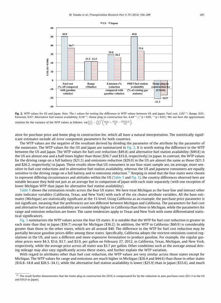
Fig. 2. WTP values for US and Japan. Note: The t values for testing the difference in WTP values between US and Japan: Fuel cost, 2.82⁄⁄⁄; Range, 0.01;Emission, 0.67; Alternative fuel station availability, 6.54⁄⁄⁄; Home plug-in construction fee, 4.44⁄⁄⁄; (⁄⁄p < 0.05, ⁄⁄⁄p < 0.01). We use here the approximate

solution for the variance of the WTP values as follows: var bibj

� �¼ bj

bi

� �2varðbi Þ

b2iþ varðbjÞ

b2j� 2covðbi ;bj Þ

bibj

� �.

M. Tanaka et al. / Transportation Research Part A 70 (2014) 194–209 201

ative for purchase price and home plug-in construction fee, which all have a natural interpretation. The statistically signif-icant estimates include all error component parameters for both countries.

The WTP values are the negative of the resultant derived by dividing the parameter of the attribute by the parameter ofthe numeraire. The WTP values for the US and Japan are summarized in Fig. 2. It is worth noting the difference in the WTPbetween the US and Japan. The WTP values for fuel cost reduction ($49.8) and alternative fuel station availability ($49.8) inthe US are almost one and a half times higher than those ($36.7 and $33.6, respectively) in Japan. In contrast, the WTP valuesfor the driving range on a full battery ($21.5) and emissions reduction ($29.0) in the US are almost the same as those ($21.5and $26.2, respectively) in Japan. These results show that US consumers in our four-state sample are, on average, more sen-sitive to fuel cost reductions and to alternative fuel station availability, whereas the US and Japanese consumers are equallysensitive to the driving range on a full battery and to emissions reduction.13 Keeping in mind that the four states were chosento represent differing circumstances and attitudes within the US (Table 5 and Fig. 3), the country differences observed here arenotable because they hold not just as an average but in comparison of Japan with each state separately (with one exception oflower Michigan WTP than Japan for alternative fuel station availability).

Table 5 shows the estimation results across the four US states. We here treat Michigan as the base line and interact otherstate indicator variables (California, Texas, and New York) with each of the six choice attribute variables. All the base esti-mates (Michigan) are statistically significant at the 1% level. Using California as an example, the purchase price parameter isnot significant, meaning that the preferences are not different between Michigan and California. The parameters for fuel costand alternative fuel station availability are considerably higher in California than those in Michigan, while the parameters forrange and emission reduction are lower. The same tendencies apply to Texas and New York with some differentiated statis-tical significances.

Fig. 3 summarizes the WTP values across the four US states. It is notable that the WTP for fuel cost reduction is greater ineach state than that in Japan ($36.7) except for Michigan ($36.2). In addition, the WTP in California ($60.9) is considerablygreater than those in the other states, which are all around $40. The difference in the WTP for fuel cost reduction may bepartially because gasoline prices differ among these states. Specifically, California adopts the strictest emissions control reg-ulations in the US, and uses a different and more expensive formulation to produce gasoline. For example, the regular gas-oline prices were $4.3, $3.6, $3.7, and $3.9, per gallon on February 27, 2012, in California, Texas, Michigan, and New York,respectively, while the average price across all states was $3.7 per gallon. Other conditions such as the average annual driv-ing mileage may also vary significantly across these states, and further explain the WTP variation.

With regard to attributes other than fuel cost reduction, the WTP values are very similar across those states except forMichigan. The WTP values for range and emissions are much higher in Michigan ($26.4 and $44.6) than those in other states($16.8–18.8 and $26.5–34.1), while the alternative fuel station availability is lower ($25.9) than in Japan ($33.6), and much

13 The result further demonstrates that the home plug-in construction fee ($10) is compensated for by the reduction in auto purchase costs ($21.3 in the USand $16.9 in Japan).

Table 5Estimation results across four US states.

US respondents

Coeff. Std. Err. WTP (US$)

<non random parameters: Base = Michigan>ASC for EV 5.62129 0.16858⁄⁄⁄ –ASC for PHEV 6.80828 0.16816⁄⁄⁄ –ASC for gasoline vehicles 5.84320 0.13605⁄⁄⁄ –Purchase price (US$) �0.00030 0.00623⁄⁄⁄ –Fuel cost (% off compared with gasoline vehicles) 0.01074 0.00175⁄⁄⁄ 36.22Range (miles) 0.00078 0.00011⁄⁄⁄ 2.64Emission reduction (% reduction compared with gasoline vehicles) 0.01322 0.00158⁄⁄⁄ 44.59

Alternative fuel station availability(% of existing gas stations) 0.00768 0.00068⁄⁄⁄ 25.90Home plug-in construction fee (US$100) �0.07092 0.00406⁄⁄⁄ �239.19

<Interaction term: California>Purchase price (US$) 0.00000 0.00001 –Fuel cost (% off compared with gasoline vehicles) 0.00727 0.00240⁄⁄⁄ 24.67Range (miles) �0.00026 0.00012⁄⁄ �0.87Emission reduction (% reduction compared with gasoline vehicles) �0.00376 0.00207⁄ �12.76

Alternative fuel station availability(% of existing gas stations) 0.00793 0.00119⁄⁄⁄ 26.91Home plug-in construction fee (US$100) 0.01820 0.00556⁄⁄⁄ 61.76

<Interaction term: Texas>Purchase price (US$) 0.00000 0.00001 –Fuel cost (% off compared with gasoline vehicles) 0.00264 0.00234 8.82Range (miles) �0.00029 0.00013⁄⁄ �0.96Emission reduction (% reduction compared with gasoline vehicles) �0.00313 0.00210 �10.46

Alternative fuel station availability(% of existing gas stations) 0.00743 0.00120⁄⁄⁄ 24.83Home plug-in construction fee (US$100) 0.01080 0.00566⁄ 36.09

<Interaction term: New York>Purchase price (US$) 0.00000 0.00001 �Fuel cost (% off compared with gasoline vehicles) 0.00309 0.00234 10.57Range (miles) �0.00022 0.00013⁄ �0.77Emission reduction (% reduction compared with gasoline vehicles) �0.00528 0.00207⁄⁄ �18.07

Alternative fuel station availability(% of existing gas stations) 0.00732 0.00117⁄⁄⁄ 25.05Home plug-in construction fee (US$100) 0.00723 0.00568 24.74

<Standard deviation of error component>EV 1.60359 0.0363⁄⁄⁄ –PHEV 0.09710 0.0641 –Gasoline vehicles 3.90483 0.0827⁄⁄⁄ –Not buy 3.61312 0.0670⁄⁄⁄ –Number of obs. 33616McFadden Pseudo R-squared 0.3704Log likelihood function �29340.92

Note: ASC denotes alternative specific constant. The percentage variables (fuel cost, emission reduction, fuel station availability) are on a scale of 0-100. ⁄⁄⁄, ⁄⁄

and ⁄ denote significance at the 1%, 5% and 10% levels, respectively

202 M. Tanaka et al. / Transportation Research Part A 70 (2014) 194–209

lower than each of the other three states ($50.7–52.9). It is interesting that the WTP for emissions reduction in California issimilar to the other states, despite consumers in California reputedly being more aware of environmental protection thanthose in other states.

5. Implications for future diffusion

This section discusses the numerical implications for EV/PHEV market shares (percent of car purchases) based on the esti-mates obtained in Section 4. For this purpose, we insert the estimates obtained in Tables 5 and 6 into the ECML choice prob-abilities represented in Eq. (2). We consider three different states of the world, or scenarios:

� A base case Scenario 1 with relatively realistic attribute levels attainable with current technologies.� Scenario 2 with a purchase price reduction for an EV/PHEV, while the other attribute levels are the same as in Scenario 1.

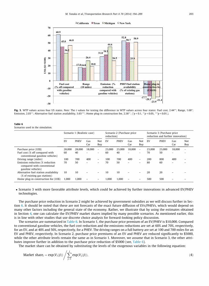
Table 6Scenarios used in the simulation.

Scenario 1 (Realistic case) Scenario 2 (Purchase pricereduction)

Scenario 3 (Purchase pricereduction and further innovation)

EV PHEV GasCar

NotBuy

EV PHEV GasCar

NotBuy

EV PHEV GasCar

NotBuy

Purchase price (US$) 28,000 28,000 18,000 – 23,000 23,000 18,000 – 23,000 23,000 18,000 –Fuel cost (% off compared with

conventional gasoline vehicles)60 40 – – 60 40 – – 70 50 – –

Driving range (miles) 100 700 400 – 100 700 400 – 200 800 400 –Emission reduction (% reduction

compared with conventionalgasoline vehicles)

70 50 – – 70 50 – – 80 60 – –

Alternative fuel station availability(% of existing gas stations)

10 10 – – 10 10 – – 20 20 – –

Home plug-in construction fee (US$) 1,000 1,000 – – 1,000 1,000 – – 500 500 – –

60.9

17.8

31.8

52.8

-17.7

45.0

16.8

34.1

50.7

-20.3

36.2

26.4

44.6

25.9

-23.9

46.8

18.8

26.5

50.9

-21.4-30

-20

-10

0

10

20

30

40

50

60

70

Fuel cost(% off compared

with gasoline vehicles)

Range(10 miles)

Emission (% reduction

compared with gasoline vehicles)

PHEVfuel station availability

(% of existing gas stations)

Home plug-in construction fee

(US$10)

US$

($1=

¥100

)

California Texas Michigan New York

Fig. 3. WTP values across four US states. Note: The t values for testing the difference in WTP values across four states: Fuel cost, 2.44⁄⁄; Range, 1.68⁄;Emission, 2.03⁄⁄; Alternative fuel station availability, 5.65⁄⁄⁄; Home plug-in construction fee, 2.58⁄⁄. (⁄p < 0.1, ⁄⁄p < 0.05, ⁄⁄⁄p < 0.01.).

M. Tanaka et al. / Transportation Research Part A 70 (2014) 194–209 203

� Scenario 3 with more favorable attribute levels, which could be achieved by further innovations in advanced EV/PHEVtechnologies.

The purchase price reduction in Scenario 2 might be achieved by government subsidies as we will discuss further in Sec-tion 6. It should be noted that these are not forecasts of the exact future diffusion of EVs/PHEVs, which would depend onmany other factors including the general state of the economy. Rather, we illustrate that by using the estimates obtainedin Section 4, one can calculate the EV/PHEV market shares implied by many possible scenarios. As mentioned earlier, thisis in line with other studies that use discrete choice analysis for forward-looking policy discussion.

The scenarios are summarized in Table 6. In Scenario 1, the purchase price premium of an EV/PHEV is $10,000. Comparedto conventional gasoline vehicles, the fuel cost reduction and the emissions reductions are set at 60% and 70%, respectively,for an EV, and at 40% and 50%, respectively, for a PHEV. The driving ranges on a full battery are set at 100 and 700 miles for anEV and PHEV, respectively. In Scenario 2, purchase price premiums of an EV and PHEV are reduced significantly to $5000,while the other attribute levels remain the same as in Scenario 1. Moreover, we assume that in Scenario 3, the other attri-butes improve further in addition to the purchase price reduction of $5000 (see, Table 6).

The market share can be obtained by substituting the levels of the exogenous variables in the following equation:

Market sharei ¼ expðViðbÞÞXJ

j¼1

expðVjðbÞÞ,

; ð4Þ

(a)

3.6%

5.6%

10.4%

20.7%

70.0%

58.0%

16.1%

15.7%

0% 20% 40% 60% 80% 100%

USA

Japan

EV PHEV Gas Car Not Buy

(b)

10.7%

14.4%

31.1%

53.7%

47.3%

25.1%

10.9%

6.8%

0% 20% 40% 60% 80% 100%

USA

Japan

EV PHEV Gas Car Not Buy

(c)

15.6%

17.2%

45.2%

64.3%

31.9%

14.6%

7.3%

3.9%

0% 20% 40% 60% 80% 100%

USA

Japan

EV PHEV Gas Car Not Buy

Fig. 4. Market shares in US and Japan. (a) Base case scenario 1 (realistic case), (b) Scenario 2 (Purchase price reduction) and (c) Scenario 3 (Furtherinnovation with purchase price reduction).

204 M. Tanaka et al. / Transportation Research Part A 70 (2014) 194–209

which is the normal logit formula, as shown in earlier estimations. We calculate the percentage of those who would purchasean EV, PHEV, or conventional gasoline vehicle as the expected market share in each case. We here use the estimated coef-ficients for the alternative constants, and we emphasize the market share changes caused by simulating the alternative sce-narios within each of our studied jurisdictions (rather than across them).14

Fig. 4(a)–(c) show the market shares obtained by applying the scenario attribute levels to our earlier estimated equation:the expected percentages of new car purchases for EVs, PHEVs and conventional gasoline vehicles at the specified attributelevels. In the base case Scenario 1, conventional gasoline vehicles still dominate at 70.0% and 58.0% in the US and Japan,respectively. More specifically, the very high purchase price premium of EVs/PHEVs prevents alternative vehicles from dif-fusing more broadly. However, we find that PHEVs do begin to penetrate the US and Japanese markets with shares of 10.4%and 20.7%, respectively. On the other hand, EVs appear not very popular in both countries with market shares of only 3.6%and 5.6% in the US and Japan, respectively.15

In Scenario 2, the purchase price premium of EVs/PHEVs is reduced significantly to $5000. As illustrated in Fig. 4(b), theEV/PHEV market shares reach 41.8% and 68.1% in the US and Japan, respectively. The PHEV share is 53.7% in Japan, while theshare is 31.1% in the US. As in the base case Scenario 1, PHEVs would be more attractive to Japanese consumers. The EVshares are 10.7% and 14.4% in the US and Japan, respectively. In Scenario 3 with further innovations, the EV/PHEV shares

14 Although the number of respondents is almost the same (4202 for US and 4000 for Japan) and they responded to the same eight questions, the values ofMcFadden Pseudo R2 are slightly different (0.3378 for US and 0.4223 for Japan).

15 Note that ‘‘Not Buy’’ means the respondents will not buy any of those vehicles with the ‘‘specified attribute levels.’’ This does not necessarily imply that theywill not own any vehicle. For example, the respondents who indicated ‘‘Not Buy’’ might still purchase less expensive gasoline vehicles in the used-car market.

(a)

5.2%

3.8%

3.3%

3.5%

13.1%

10.2%

10.3%

10.1%

66.6%

68.9%

71.3%

71.1%

15.1%

17.1%

15.1%

15.2%

0% 20% 40% 60% 80% 100%

CAL

TEX

MIC

NY

EV PHEV Gas Car Not Buy

(b)

14.1%

11.5%

9.9%

10.5%

35.4%

30.6%

31.1%

30.0%

41.2%

46.4%

48.7%

49.0%

9.3%

11.5%

10.3%

10.5%

0% 20% 40% 60% 80% 100%

CAL

TEX

MIC

NY

EV PHEV Gas Car Not Buy

(c)

19.3%

16.5%

14.4%

15.3%

48.2%

43.8%

45.1%

43.6%

26.6%

31.8%

33.4%

33.9%

6.0%

7.9%

7.0%

7.2%

0% 20% 40% 60% 80% 100%

CAL

TEX

MIC

NY

EV PHEV Gas Car Not Buy

Fig. 5. Market shares across four US states. (a) Base case scenario 1 (realistic case), (b) Scenario 2 (Purchase price reduction) and (c) Scenario 3 (Furtherinnovation with purchase price reduction).

M. Tanaka et al. / Transportation Research Part A 70 (2014) 194–209 205

reach 60.8% and 81.5% in the US and Japan, respectively, as shown in Fig. 4(c). In this scenario of technological advances withpurchase price reduction, a high penetration of alternative fuel vehicles might be achieved in both countries.

Fig. 5(a)–(c) show the details of the four states in the US. Notably, California leads the way in deploying alternative fuelvehicles. Specifically, the EV share is the greatest in California for all scenarios because of the high WTP for fuel costreductions.

6. Further policy discussion

We mentioned in our introduction that it is the explicit goal of the US and Japanese governments, as well as many othergovernments, to increase the number of greener, alternative fuel vehicles on the roads. Policies that may serve this purpose

206 M. Tanaka et al. / Transportation Research Part A 70 (2014) 194–209

can work from the supply side, as with new emission standards that manufacturers must meet, and from the demand side toinfluence the buying choices of consumers. The investigation of this article has been on the demand side, to understand bet-ter the concerns, considerations and likely tradeoffs among vehicle attributes of consumers. Thus our results apply mostdirectly to the demand side policies that governments may be using or considering.

There are actually quite a broad range of demand-side policies that either are or could be in use. We have already men-tioned rebates for the purchase of these vehicles, in effect in Japan through tax exemptions equal to about 5.7% of the pur-chase price and in the US for up to $7500 per vehicle and an additional $2500 in the state of California. In addition, there maybe rebates or subsidies for the purchase or installation of home charging equipment. In the San Francisco area, the local BayArea Air Quality Management District is offering a free charger and up to a $1200 installation credit for as many as 2750residents. There are policies to make trip-making in these vehicles easier, notably to facilitate convenient access to rapid-charging stations in various locations like those along highways. California allows alternative vehicles unlimited free accessto the High Occupancy Vehicle lanes of its highways. Acting through the electric utilities, governments may act to providespecial low-cost electric vehicle charging rates. Government could also offer parking incentives for these vehicles.

A full discussion of these policies is of course beyond the scope of this article. However, we wish to highlight here thegeneral potential of the methods used in this research to strengthen policy analysis. Economics is used in policy analysisat both the theoretical and empirical levels. Because actual policy choices are intended to affect the future, it is often thecase that some policy alternatives have not yet been tried and there is therefore no direct empirical evidence on its effectsfrom actual behavioral responses. As the survey-based methodology of conjoint analysis continues to improve, it does havethe potential to provide useful empirical evidence in these forward-looking situations. Furthermore, when policies do go intoeffect, there is the opportunity to compare the results from the earlier conjoint analysis with the actual behavioralresponses—thus providing important evidence that over time can be used to improve the methodology.

At the theoretical level for policy with respect to increasing the diffusion of alternative fuel vehicles, the arguments forpolicy interventions are generally strongest when they successfully address specific market failures.16 The private sector canitself be expected to provide many of these services mentioned above as potential policy levers, such as convenient chargingstations. Tesla, for example, has already set up 6 free charging stations along California freeways for its Model S vehicles,and plans to put up dozens more in California and eventually to cover most of the U.S.17 As there may be a ‘‘chicken andegg’’ problem as to which comes first (the vehicles or the charging stations), it may be appropriate in some circumstancesfor policy to help initiate these services. The case for vehicle purchase incentives comes primarily from the behavioral econom-ics literature. That literature suggests many consumers may suffer from ‘‘sticker shock’’ or the ‘‘energy paradox’’ (Jaffe andStavins, 1994) where they perceive immediately the higher upfront cost of an EV or PHEV vehicle (or other energy-efficientdurable goods like refrigerators), but have difficulty recognizing, knowing or understanding the expected present value of fuelsavings over time—leading them to under invest in clean energy investments. The electricity rate policy is more complex. Fewelectricity rates are actually set close to their marginal costs, and there are very strong arguments that these rates should betime-differentiated which would encourage off-peak charging.18 However, the social cost of electricity is the same regardlessof the device that it runs, so it would be inefficient to have a special rate that applies to only one type of device.

It is worthwhile noting that a $5000 policy increase in vehicle purchase incentives would have the same effect as a $5000purchase price reduction resulting from market forces (if the incentive is applied at the time of purchase). To get a sense ofthe effect of such a policy increase, consider the Scenario 1 finding that only 10.4% of households in the four-state US samplewould purchase a PHEV. If the purchase incentive were increased by $5000 holding all other factors constant at the Scenario1 level, our estimates imply this would cause PHEV purchases to rise to 31.1% of households. This estimate of a substantialeffect can in the future be compared with other econometric estimates resulting from studies of actual purchase decisions.

7. Concluding remarks

This paper conducted a comparative discrete choice analysis to estimate consumers’ willingness to pay for EVs and PHEVsbased on the same online stated preference survey carried out in both the US and Japan in 2012. We also carried out a com-parative analysis across the four US states that comprised the US sample. Our findings showed that the WTP values for fuelcost reduction ($49.8) and alternative fuel station availability ($49.8) in the US are almost one and a half times higher thanthose in Japan ($36.7 and $33.6, respectively). In contrast, the WTP values for the driving range on a full battery ($21.5) andemissions reduction ($29.0) in the US are almost the same as those in Japan ($21.5 and $26.2, respectively). These resultsimply that US consumers are, on average, more sensitive to fuel cost reductions and to alternative fuel station availability,while the US and Japanese consumers are equally sensitive to the driving range on a full battery and to emissions reduction.With regard to the comparative analysis across the four US states, we found that the WTP for a fuel cost reduction in Cal-ifornia ($60.9) is 30–70% higher than those in the other three states ($36–47). Furthermore, we conducted a numerical sim-ulation of EV/PHEV diffusion based on the estimates obtained in the discrete choice analysis. In the base case scenario withrelatively realistic attribute levels, conventional gasoline vehicles still dominate both in the US and Japan. However, in an

16 For a review of these as they affect energy-efficiency decisions, see Gillingham et al. (2009).17 See the Business Week report of the Tesla announcement posted by Ashlee Vance on September 24, 2012 at http://www.businessweek.com/articles/2012-

09-25/tesla-fires-up-solar-powered-charging-stations.18 See for example Friedman (2011).

M. Tanaka et al. / Transportation Research Part A 70 (2014) 194–209 207

innovation scenario with a significant purchase price reduction, we observed a high penetration of alternative fuel vehiclesin both countries. Our estimates imply that government purchase price subsidies can have a significant effect on the diffu-sion of these vehicles: we estimated that an increase of $5000 in such a subsidy would increase the market share of PHEVsfrom 10.4% in the US under Scenario 1 to 31.1%. As a final remark, we acknowledge that our results are all based on a dataanalysis of stated preferences, which should be compared with the results of a revealed preference data analysis in thefuture. The results of such an analysis remain an important source of improvements for the stated preference methodology.

Acknowledgement

We are grateful to Aleka Seville for her valuable support. We also wish to thank two anonymous referees for their helpfulcomments. The usual disclaimers apply.

Appendix A. Individual/household heterogeneity analysis

The analysis presented in this study can be developed to address individual and household heterogeneity. While our pri-mary interest has been in cross-country and state comparisons, we present a simple model based on the idea that individual

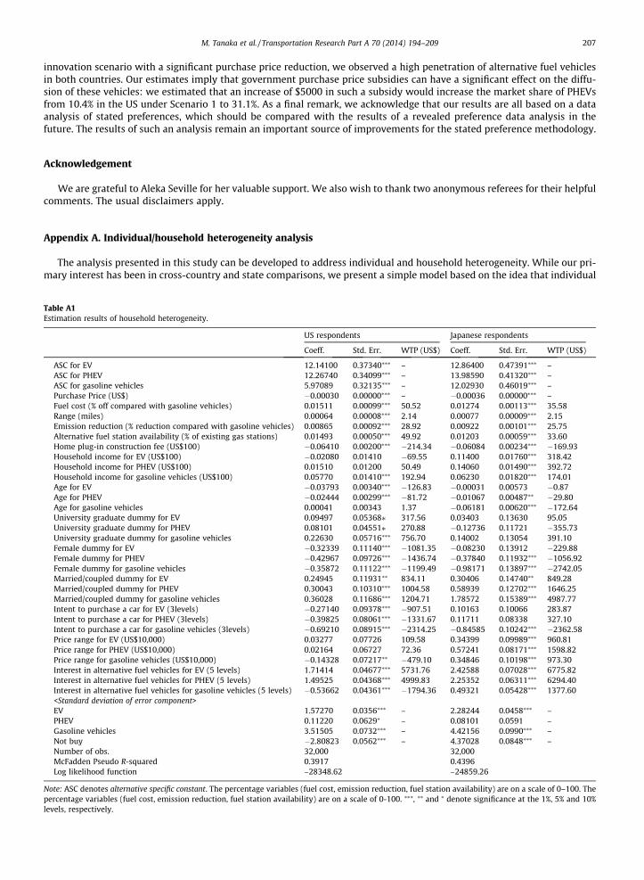
Table A1Estimation results of household heterogeneity.

US respondents Japanese respondents

Coeff. Std. Err. WTP (US$) Coeff. Std. Err. WTP (US$)

ASC for EV 12.14100 0.37340⁄⁄⁄ – 12.86400 0.47391⁄⁄⁄ –ASC for PHEV 12.26740 0.34099⁄⁄⁄ – 13.98590 0.41320⁄⁄⁄ –ASC for gasoline vehicles 5.97089 0.32135⁄⁄⁄ – 12.02930 0.46019⁄⁄⁄ –Purchase Price (US$) �0.00030 0.00000⁄⁄⁄ – �0.00036 0.00000⁄⁄⁄ –Fuel cost (% off compared with gasoline vehicles) 0.01511 0.00099⁄⁄⁄ 50.52 0.01274 0.00113⁄⁄⁄ 35.58Range (miles) 0.00064 0.00008⁄⁄⁄ 2.14 0.00077 0.00009⁄⁄⁄ 2.15Emission reduction (% reduction compared with gasoline vehicles) 0.00865 0.00092⁄⁄⁄ 28.92 0.00922 0.00101⁄⁄⁄ 25.75Alternative fuel station availability (% of existing gas stations) 0.01493 0.00050⁄⁄⁄ 49.92 0.01203 0.00059⁄⁄⁄ 33.60Home plug-in construction fee (US$100) �0.06410 0.00200⁄⁄⁄ �214.34 �0.06084 0.00234⁄⁄⁄ �169.93Household income for EV (US$100) �0.02080 0.01410 �69.55 0.11400 0.01760⁄⁄⁄ 318.42Household income for PHEV (US$100) 0.01510 0.01200 50.49 0.14060 0.01490⁄⁄⁄ 392.72Household income for gasoline vehicles (US$100) 0.05770 0.01410⁄⁄⁄ 192.94 0.06230 0.01820⁄⁄⁄ 174.01Age for EV �0.03793 0.00340⁄⁄⁄ �126.83 �0.00031 0.00573 �0.87Age for PHEV �0.02444 0.00299⁄⁄⁄ �81.72 �0.01067 0.00487⁄⁄ �29.80Age for gasoline vehicles 0.00041 0.00343 1.37 �0.06181 0.00620⁄⁄⁄ �172.64University graduate dummy for EV 0.09497 0.05368⁄ 317.56 0.03403 0.13630 95.05University graduate dummy for PHEV 0.08101 0.04551⁄ 270.88 �0.12736 0.11721 �355.73University graduate dummy for gasoline vehicles 0.22630 0.05716⁄⁄⁄ 756.70 0.14002 0.13054 391.10Female dummy for EV �0.32339 0.11140⁄⁄⁄ �1081.35 �0.08230 0.13912 �229.88Female dummy for PHEV �0.42967 0.09726⁄⁄⁄ �1436.74 �0.37840 0.11932⁄⁄⁄ �1056.92Female dummy for gasoline vehicles �0.35872 0.11122⁄⁄⁄ �1199.49 �0.98171 0.13897⁄⁄⁄ �2742.05Married/coupled dummy for EV 0.24945 0.11931⁄⁄ 834.11 0.30406 0.14740⁄⁄ 849.28Married/coupled dummy for PHEV 0.30043 0.10310⁄⁄⁄ 1004.58 0.58939 0.12702⁄⁄⁄ 1646.25Married/coupled dummy for gasoline vehicles 0.36028 0.11686⁄⁄⁄ 1204.71 1.78572 0.15389⁄⁄⁄ 4987.77Intent to purchase a car for EV (3levels) �0.27140 0.09378⁄⁄⁄ �907.51 0.10163 0.10066 283.87Intent to purchase a car for PHEV (3levels) �0.39825 0.08061⁄⁄⁄ �1331.67 0.11711 0.08338 327.10Intent to purchase a car for gasoline vehicles (3levels) �0.69210 0.08915⁄⁄⁄ �2314.25 �0.84585 0.10242⁄⁄⁄ �2362.58Price range for EV (US$10,000) 0.03277 0.07726 109.58 0.34399 0.09989⁄⁄⁄ 960.81Price range for PHEV (US$10,000) 0.02164 0.06727 72.36 0.57241 0.08171⁄⁄⁄ 1598.82Price range for gasoline vehicles (US$10,000) �0.14328 0.07217⁄⁄ �479.10 0.34846 0.10198⁄⁄⁄ 973.30Interest in alternative fuel vehicles for EV (5 levels) 1.71414 0.04677⁄⁄⁄ 5731.76 2.42588 0.07028⁄⁄⁄ 6775.82Interest in alternative fuel vehicles for PHEV (5 levels) 1.49525 0.04368⁄⁄⁄ 4999.83 2.25352 0.06311⁄⁄⁄ 6294.40Interest in alternative fuel vehicles for gasoline vehicles (5 levels) �0.53662 0.04361⁄⁄⁄ �1794.36 0.49321 0.05428⁄⁄⁄ 1377.60<Standard deviation of error component>EV 1.57270 0.0356⁄⁄⁄ – 2.28244 0.0458⁄⁄⁄ –PHEV 0.11220 0.0629⁄ – 0.08101 0.0591 –Gasoline vehicles 3.51505 0.0732⁄⁄⁄ – 4.42156 0.0990⁄⁄⁄ –Not buy �2.80823 0.0562⁄⁄⁄ – 4.37028 0.0848⁄⁄⁄ –Number of obs. 32,000 32,000McFadden Pseudo R-squared 0.3917 0.4396Log likelihood function –28348.62 –24859.26

Note: ASC denotes alternative specific constant. The percentage variables (fuel cost, emission reduction, fuel station availability) are on a scale of 0–100. Thepercentage variables (fuel cost, emission reduction, fuel station availability) are on a scale of 0-100. ⁄⁄⁄, ⁄⁄ and ⁄ denote significance at the 1%, 5% and 10%levels, respectively.

208 M. Tanaka et al. / Transportation Research Part A 70 (2014) 194–209

decisions can also be understood as a function of demographic characteristics and consumer consciousness. The followingvariables are included in the model:

� Household income (unit: $100 increase)� Age� University graduate dummy� Female dummy� Married/cohabiting dummy� Intent to purchase a car within the next five years (1 = buy, 2 = lease, 3 = not to buy)� Price range for purchasing a next vehicle (unit: $10,000 increase)� Interest in alternative fuel vehicles (1 = not interested . . . 5 = very interested)

The estimation results are presented in Table A1.19 The WTP values are measured for each alternative based on the baseline(not buy) alternatives. Some observations can be summarized as follows:

� Household income considerably influences the WTP values for the purchase of EVs, PHEVs, and gasoline vehicles in Japan.For example, a household with $100 higher income indicates that they would pay more to purchase an EV or PHEV ($318and $393 for Japan, respectively). Unexpectedly, however, the EV and PHEV premiums are not necessarily high becausethe WTP values are also high for purchasing gasoline vehicles ($193 for the US and $174 for Japan). This simply meansthat a rich family can afford to buy a more expensive vehicle.� Age has a negative effect on the WTP values for purchasing an EV, PHEV, and gasoline vehicle. However, it is interesting to

note that the impact is asymmetric between the US and Japan: the values for EV are �$127 for the US and �$1 for Japan,while the values for gasoline vehicles are $1 for the US and �$173 for Japan.� University graduates have a higher WTP for the purchase of EVs, PHEVs, and gasoline vehicles in the US ($318, $271, and

$757, respectively). On the other hand, such graduates have no statistically significant preferences in Japan ($95, �$356,and $391, respectively).� Females have negative WTP values for the purchase of EVs, PHEVs, and gasoline vehicles in the US (�$1081, �$1437, and�$1199, respectively). This implies that females are generally negative about purchasing vehicles but are much less neg-ative about EVs and PHEVs. The same tendencies are observed in Japan (�$230, �$1057, and �$2742, respectively).� Married/cohabiting couples have positive WTP values for the purchase of EVs, PHEVs, and gasoline vehicles in the US

($834, $1005, and $1205, respectively). This implies that married/cohabiting couples are generally positive about the pur-chase of PHEVs and gasoline vehicles but are much less positive about EVs. The same tendencies are obvious in Japan($849, $1646, and $4988, respectively).� Households that intend to purchase a car within the next five years have large WTP values for the purchase of a gasoline

vehicle in the US ($2314), but relatively smaller values for an EV and PHEV ($908 and $1332, respectively). Again, thesame tendencies are obvious in Japan (�$284, �$327, and $2363, respectively).� Households considering purchasing an expensive vehicle have positive but not statistically significant WTP values for an

EV and PHEV ($110 and $72, respectively) and a significantly negative WTP value for gasoline vehicles in the US (�$479).It is remarkable that households considering purchasing an expensive vehicle have a large WTP value for EVs, PHEVs andgasoline vehicles in Japan ($961, $1599, and $973, respectively).� Finally, households that are interested in an alternative fuel vehicle have very large WTP values for the purchase of an EV

and PHEV ($5732 and $5000, respectively) but a negative WTP value for gasoline vehicles in the US (�$1794). Similar ten-dencies are observed in Japan ($6776, $6294, and $1378, respectively).

References

Achtnicht, M., Buhler, G., Hermeling, C., 2012. The impact of fuel availability on demand for alternative-fuel vehicles. Transp. Res. Part D 17, 262–269.Ahn, J., Jeong, G., Kim, Y., 2008. A forecast of household ownership and use of alternative fuel vehicles: a multiple discrete-continuous choice approach.

Energy Econ. 30, 2091–2104.Axsen, J., Mountain, D.C., Jaccard, M., 2009. Combining stated and revealed choice research to simulate the neighbor effect: the case of hybrid-electric

vehicles. Resour. Energy Econ. 31, 221–238.Beggs, S., Cardell, S., Hausman, J., 1981. Assessing the potential demand for electric cars. J. Economet. 16, 1–19.Ben-Akiva, M., Bolduc D., Walker J., 2001. Specification, estimation and identification of the logit kernel (or continuous mixed logit) model. Department of

Civil Engineering, MIT, Working Paper.Bhat, C., 2001. Quasi-random maximum simulated likelihood estimation of the mixed multinomial logit model. Transp. Res. Part B 35, 677–693.Brownstone, D., Train, K.E., 1999. Forecasting new product penetration with flexible substitution patterns. J. Economet. 89, 109–129.Brownstone, D., Bunch, D.S., Train, K.E., 2000. Joint mixed logit models of stated and revealed preferences for alternative-fuel vehicles. Transp. Res. Part B 34,

315–338.Bunch, D.S., Bradley, M., Golob, T.F., Kitamura, R., Occhiuzzo, G.P., 1993. Demand for clean-fuel vehicles in California: a discrete-choice stated preference

pilot project. Transp. Res. Part A 27 (3), 237–253.Calfee, J.E., 1985. Estimating the demand for electric automobiles using disaggregated probabilistic choice analysis. Transp. Res. Part B 19 (4), 287–301.

19 See, for example, Daziano and Chiew (2012) for a detailed review of past studies.

M. Tanaka et al. / Transportation Research Part A 70 (2014) 194–209 209

Center for Sustainable Energy, 2013. 2012 Annual Report.Dagsvik, J.K., Wetterwald, D.G., Wennemo, T., Aaberge, R., 2002. Potential demand for alternative fuel vehicles. Transp. Res. Part B 36, 361–384.Daziano, R.A., Bolduc, D., 2013. Incorporating pro-environmental preferences toward green automobile technologies through a Bayesian Hybrid Choice

Model. Transport. A: Transp. Sci. 9 (1), 74–106.Daziano, R.A., Chiew, E., 2012. Electric vehicles rising from the dead: data needs for forecasting consumer response toward sustainable energy sources in

personal transportation. Energy Policy 51, 876–894.Ewing, G.O., Sarigöllü, E., 1998. Car fuel-type choice under travel demand management and economic incentives. Transp. Res. Part D 3 (6), 429–444.Ewing, G., Sarigöllü, E., 2000. Assessing consumer preferences for clean-fuel vehicles: a discrete choice experiment. J. Public Policy Mark. 19 (1), 106–118.Friedman, L.S., 2011. The Importance of marginal cost electricity pricing to the success of greenhouse gas reduction programs. Energy Policy 39 (11), 7347–

7360.Gillingham, G., Newell, R.G., Palmer, K., 2009. Energy efficiency economics and policy. Ann. Rev. Resour. Econ. Ann. Rev. 1 (1), 597–620.Graham-Rowe, E., Gardner, B., Abraham, C., Skippon, S., Dittmar, H., Hutchins, R., Stannard, J., 2012. Mainstream consumers driving plug-in battery-electric

and plug-in hybrid electric cars: a qualitative analysis of responses and evaluations. Transp. Res. Part A 46 (1), 140–153.Hackbarth, A., Madlener, R., 2013. Consumer preferences for alternative fuel vehicles: a discrete choice analysis. Transp. Res. Part D 25, 5–17.Halton, J.E., 1960. On the efficiency of certain quasi-random sequences of points in evaluating multi-dimensional integrals. Numer. Math. 2, 84–90.Hidrue, M.K., Parsons, G.R., Kempton, W., Gardner, M.P., 2011. Willingness to pay for electric vehicles and their attributes. Resour. Energy Econ. 33, 686–705.Hess, S., Fowler, M., Adler, T., Bahreinian, A., 2012. A joint model for vehicle type and fuel type choice: evidence from a cross-nested logit study.

Transportation 39 (3), 593–625.Horne, M., Jaccard, M., Tiedemann, K., 2005. Improving behavioral realism in hybrid energy–economy models using discrete choice studies of personal

transportation decisions. Energy Econ. 27, 59–77.Ito, N., Takeuchi, K., Managi, S., 2013. Willingness to pay for the infrastructure investments for alternative fuel vehicles. Transp. Res. Part D 18, 1–8.Jaffe, A., Stavins, R., 1994. The energy paradox and the diffusion of conservation technology. Resour. Energy Econ. 16, 91–122.Japan Automobile Manufacturers Association Inc., 2012. The motor industry of Japan 2012.Karplus, V.J., Paltsev, S., Reilly, J.M., 2010. Prospects for plug-in hybrid electric vehicles in the United States and Japan: a general equilibrium analysis.

Transp. Res. Part A 44, 620–641.Krupa, J.S., Rizzo, D.M., Eppstein, M.J., Brad Lanute, D., Gaalema, D.E., Lakkaraju, K., Warrender, C.E., 2014. Analysis of a consumer survey on plug-in hybrid

electric vehicles. Transp. Res. Part A 64, 14–31.Louviere, J.J., Hensher, D.A., Swait, J.D., 2000. Stated Choice Methods: Analysis and Applications. Cambridge University Press.McFadden, D., Train, K.E., 2000. Mixed MNL models of discrete choice models of discrete response. J. Appl. Economet. 15, 447–470.Mau, P., Eyzaguirre, J., Jaccard, M., Collins-Dodd, C., Tiedemann, K., 2008. The ‘neighbor effect’: simulating dynamics in consumer preferences for new

vehicle technologies. Ecol. Econ. 68, 504–516.Musti, S., Kockelman, K.M., 2011. Evolution of the household vehicle fleet: anticipating fleet composition, PHEV adoption and GHG emissions in Austin,

Texas. Transp. Res. Part A 45 (8), 707–720.Potoglou, D., Kanaroglou, P.S., 2007. Household demand and willingness to pay for clean vehicles. Transp. Res. Part D 12, 264–274.Qian, L., Soopramanien, D., 2011. Heterogeneous consumer preferences for alternative fuel cars in China. Transp. Res. Part D 16, 607–613.Revelt, D., Train, K.E., 1998. Mixed logit with repeated choices: households’ choices of appliance efficiency level. Rev. Econ. Stat. 80, 647–657.Segal, R., 1995. Forecasting the market for electric vehicles in California using conjoint analysis. Energy J. 16 (3), 89–111.Train, K.E., 2003. Discrete Choice Methods with Simulation. Cambridge University Press.Ziegler, A., 2012. Individual characteristics and stated preferences for alternative energy sources and propulsion technologies in vehicles: a discrete choice

analysis for Germany. Transp. Res. Part A 46, 1372–1385.