MNRAS 000, 1–20 (2019) Preprint 7 March 2019 Compiled using MNRAS LATEX style file v3.0

Transverse kinematics of the Galactic bar-bulge from VVV and Gaia

Jason L. Sanders,1? Leigh Smith,1,2 N. Wyn Evans,1 Philip Lucas21Institute of Astronomy, University of Cambridge, Madingley Rd, Cambridge, CB3 0HA, UK2School of Physics, Astronomy and Mathematics, University of Hertfordshire, College Lane, Hatfield AL10 9AB, UK

Accepted XXX. Received YYY; in original form ZZZ

ABSTRACTWe analyse the kinematics of the Galactic bar-bulge using proper motions from the ESOpublic survey Vista Variables in the Via Lactea (VVV) and the second Gaia data release. Gaiahas provided some of the first absolute proper motions within the bulge and the near-infraredVVV multi-epoch catalogue complements Gaia in highly-extincted low-latitude regions. Wediscuss the relative-to-absolute calibration of the VVV proper motions using Gaia. Alonglines of sight spanning −10 < `/ deg < 10 and −10 < b/ deg < 5, we probabilistically modelthe density and velocity distributions as a function of distance of ∼ 45 million stars. Thetransverse velocities confirm the rotation signature of the bar seen in spectroscopic surveys.The differential rotation between the double peaks of the magnitude distribution confirms theX-shaped nature of the bar-bulge. Both transverse velocity components increase smoothlyalong the near-side of the bar towards the Galactic centre, peak at the Galactic centre anddecline on the far-side. The anisotropy is σ`/σb ≈ 1.1 − 1.3 within the bulk of the bar,reducing to 0.9 − 1.1 when rotational broadening is accounted for, and exhibits a clear X-shaped signature. The vertex deviation in ` and b is significant |ρ`b | . 0.2, greater on the near-side of the bar and produces a quadrupole signature across the bulge indicating approximateradial alignment. We have re-constructed the 3D kinematics from the assumption of triaxiality,finding good agreement with spectroscopic survey results. In the co-rotating frame, we findevidence of bar-supporting x1 orbits and tangential bias in the in-plane dispersion field.

Key words: Galaxy: bulge – kinematics and dynamics – structure – centre

1 INTRODUCTION

The Milky Way bulge is the only Galactic bulge which we can mapin full kinematic detail. The combination of photometric, spectro-scopic and proper motion studies admits the detailed study of indi-vidual stellar populations within the Galactic bulge, revealing theformation mechanism and subsequent evolution of this component.The favoured theoretical picture is of a dynamically-formed bar-bulge that first forms from bar instabilities in the disc before buck-ling and vertically spreading into the observed bulge component.A classical bulge component formed from early accretion may alsobe present, though this remains controversial (Shen et al. 2010; DiMatteo et al. 2015).

Large-scale photometric studies (Optical Gravitational Lens-ing Experiment [OGLE], Two Micron All-Sky Survey [2MASS],UKIRT Infrared Deep Sky Survey [UKIDSS], Vista Variables inthe Via Lactea [VVV]) of the red giants towards the Galactic centrehave produced a coherent picture of the bulge as an elongated triax-ial bar structure viewed near end-on (major axis at ∼ 30 deg to theGalactic centre line-of-sight) (Stanek et al. 1997; Saito et al. 2011;Wegg & Gerhard 2013; Simion et al. 2017). Beyond |` | ≈ 10 deg,

? E-mail: jls@cam.ac.uk (JLS), nwe@ast.cam.ac.uk (NWE)

the bar-bulge gives way to the long bar, which has been traced outto ` ∼ 40 deg (∼ 5.5 kpc, Wegg et al. 2015) and appears to becontinuously connected to the bar-bulge. This suggests both com-ponents are dynamically-linked and co-rotate though this has notbeen demonstrated conclusively.

Going beyond its structural properties, the dynamical struc-ture of the bar-bulge has been most clearly elucidated by spectro-scopic studies. The line-of-sight mean velocities from the BulgeRadial Velocity Assay (BRAVA, Kunder et al. 2012), Abundancesand Radial velocity Galactic Origins Survey (ARGOS, Ness et al.2013b), Apache Point Observatory Galactic Evolution Experiment(APOGEE, Wilson et al. 2010; Abolfathi et al. 2018), Giraffe InnerBulge Survey (GIBS, Zoccali et al. 2014) and the Gaia-ESO survey(Gilmore et al. 2012) all demonstrate the cylindrical rotation ex-pected for a dynamically-formed bulge (Howard et al. 2009). Fur-thermore, dissection of the populations by spectroscopic metallicitysuggest the presence of a classical bulge component for metal-poorpopulations (Ness et al. 2013a), whilst the metal-rich population ischaracterised by orbits typical of buckled bars (e.g., Williams et al.2016). The photometric and spectroscopic measurements have beensuccessfully modelled by Portail et al. (2017) who inferred a pat-tern speed of Ωp = (39 ± 3.5)km s−1 kpc−1 placing corotation near∼ 6 kpc consistent with the observations of the long bar.

© 2019 The Authors

arX

iv:1

903.

0200

8v1

[as

tro-

ph.G

A]

5 M

ar 2

019

2 J. L. Sanders et al.

With the arrival of data from the Gaia satellite (Gaia Collabo-ration et al. 2018), there is the opportunity to complement the spec-troscopic studies of the bar-bulge with large-scale proper motionsurveys to further pin down its dynamics and formation process.Traditionally, proper motion studies require a set of backgroundsources with assumed zero proper motion (e.g. quasars) to anchorthe proper motion zero-point. In the bulge region, high extinctionand high source density means background reference sources arehard to come by and studies have been restricted to relative propermotions, for which primarily dispersions have been measured. Theearliest proper motion study of bulge stars was undertaken bySpaenhauer et al. (1992), who extracted ∼ 400 K and M giants fromphotographic plates in Baade’s window, (`, b) = (1.02,−3.93) degfinding (σ`, σb) ≈ (115, 100) km s−1. Further ground-based studieshave focussed primarily on giant stars in other windows (Plaut’swindow and NGC 6558, Mendez et al. 1996; Vieira et al. 2007;Vásquez et al. 2013). The OGLE survey opened the possibility ofmeasuring ground-based proper motions over 45 bulge fields (Sumiet al. 2004; Rattenbury et al. 2007; Poleski et al. 2013) distributedalong b ≈ −3.5 deg and the minor axis. Rattenbury et al. (2007)quantified for the first time variation in the proper motions withGalactic coordinates finding both σ` and σb increasing towards theGalactic centre. Space-based proper motions have been measuredusing the Hubble Space Telescope (HST) for select (low extinc-tion) fields including Baade’s window (Kuijken & Rich 2002), SgrI (Kuijken & Rich 2002; Clarkson et al. 2008, 2018), NGC 6553(Zoccali et al. 2001), NGC 6528 (Feltzing & Johnson 2002) andthree minor axis fields (Soto et al. 2014). The largest HST surveywas conducted by Kozłowski et al. (2006), who measured propermotions of main sequence stars in 35 fields distributed aroundBaade’s window. The gradients of Rattenbury et al. (2007) werenot clearly reproduced by this study although the reported uncer-tainties were a factor of a few larger. To date, the coverage of thebulge by proper motion studies is sparse and, besides the study ofRattenbury et al. (2007), variation of dispersion within the bulgehas not been conclusively demonstrated requiring comparison be-tween different studies.

A number of studies have combined spectroscopy with propermotion surveys to reveal full 3D kinematics of the bulge. For in-stance, Zhao et al. (1994) combined the results of Spaenhauer et al.(1992) with radial velocity data to measure the vertex deviationof the bulge confirming its triaxiality. Further studies with spec-troscopic data have elaborated on this result (Häfner et al. 2000;Soto et al. 2007) and demonstrated the variation of kinematics withmetallicity (Babusiaux et al. 2010; Hill et al. 2011; Vásquez et al.2013) revealing the relative contributions of the bar-bulge and aclassical bulge (although for only limited fields).

The new astrometric data from the Gaia satellite (Gaia Collab-oration et al. 2018) opens the possibility of fully characterizing thetransverse velocity field of the bar-bulge. The second Gaia data re-lease provided proper motions for 1.3 billion stars with G . 21across the whole sky and so extends the limited view of previ-ous proper motion surveys. Red clump stars at the Galactic centrehave G ≈ 16, so Gaia is of limited use for highly extincted fields.However, the recent VIRAC catalogue (Smith et al. 2018) for starsin the near-infrared Ks band VVV catalogue extends the depth towhich proper motions are available in high extinction regions (asAG/AKs ≈ 15). As with previous proper motion studies of thebulge, the VIRAC catalogue produced by Smith et al. (2018) pro-vides relative proper motions i.e. the proper motions are not tied toan absolute reference frame. The Gaia second data release solvesthis issue, so for the first time absolute proper motions are avail-

able for bulge stars. In this paper, we briefly describe how absoluteproper motions are computed by using bright stars in common be-tween Gaia and VIRAC. Armed with this new proper motion cata-logue, we present the transverse velocity structure of the bar-bulge.We decompose the density and velocity moments along the line-of-sight for fields −10 < b/ deg < 5 and −10 < `/ deg < 10.

The paper is laid out as follows. Section 2 describes the abso-lute proper motion catalogue created from Gaia and VIRAC, andthe subset of data used in this study. We describe the methods em-ployed in Section 3 focussing on extinction and completeness cor-rection and the kinematic modelling employed. In Section 4, wepresent the results of our analysis, before extracting the full 3d kine-matics under the assumption of triaxiality in Section 5. We closewith our conclusions in Section 6. In a companion paper (Sanders,Smith & Evans, submitted, Paper II), we use our results to estimatethe pattern speed of the bar using the continuity equation.

2 DATA

2.1 Astrometry

The VISTA Variables in the Via Lactea (VVV) survey (Minnitiet al. 2010; Saito et al. 2012) provides two epochs of ZY JH imag-ing and many more epochs of Ks band imaging over 5 years fromthe VISTA Infrared Camera (VIRCAM), covering 560 square de-grees of the southern Galactic plane and bulge. The VVV InfraredAstrometric Catalogue version 1 (VIRAC, Smith et al. 2018) is aproper motion catalogue for ∼ 300 million sources derived fromVVV survey data. VIRAC v1 uses up to several hundred epochsof Ks band data per source by combining the overlapping VIR-CAM observations (pawprint sets) necessary to obtain continu-ous coverage over the VIRCAM 1.65 square degree field of view.VIRAC v1 astrometric accuracy varies across the survey due tovarying observing cadence and source density, but typical errorsare 0.67 mas yr−1 for 11 < Ks < 14, increasing to a few mas yr−1

at Ks = 16. One important caveat of VIRAC v1 proper motions isthat they are relative to the mean motion of the local astrometric ref-erence sources used, limiting its usefulness for studying kinematicsover large scales.

With the release of the Gaia DR2 data (Gaia Collaborationet al. 2016, 2018), it is now possible to tie the relative proper mo-tions of VIRAC v1 to an absolute reference frame using stars com-mon to both catalogues. We begin this process with VIRAC v1intermediate data, proper motions generated from astrometric fitsinside sub-arrays (each array is divided into 5 × 5 = 25 sub-arrayseach covering 2.3.3arcmin2), as these are free from the reference-frame distortions introduced by the averaging proper motion solu-tions across overlapping pawprint sets. A detailed description ofthe production of this intermediate data is provided in section 3 ofSmith et al. (2018). For each sub-array we used one of three rel-ative to absolute correction methods depending on the number ofavailable Gaia reference sources and the VVV source density. Forrelatively sparse sub-arrays with sufficient Gaia reference sources,we fit and apply a 6 coefficient linear function describing propermotion reference frame shift, skew and magnification as a functionof sub-array position. For more dense sub-arrays with relativelyfew Gaia reference sources, we simply measure the average off-sets between VIRAC and Gaia proper motions in both dimensionsand apply these to the VIRAC proper motions. For sub-arrays withvery few (< 10) available Gaia reference sources, we revert to a 6coefficient linear solution as described above but using Gaia refer-ence sources across the entire array. Potential reference sources are

MNRAS 000, 1–20 (2019)

Kinematics of the Galactic bar-bulge 3

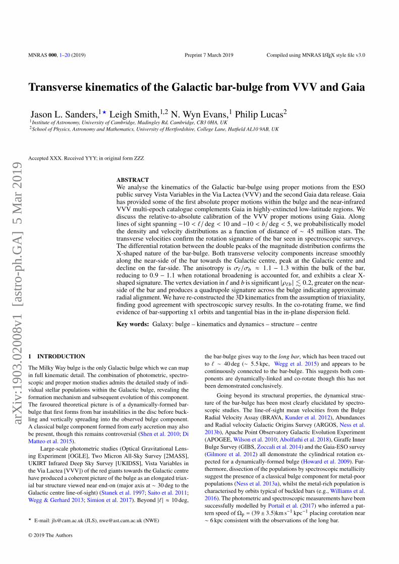
Figure 1. Relative to absolute proper motion corrections in α cos δ forsources in one pawprint set of VVV tile b371 (which contains 16 arrays).The sub-array pattern is visible, as are regions in which linear (a gradientacross the sub-array) or constant offset (flat colour in the subarray) cor-rection methods were applied depending on VVV source density and thenumber of available Gaia counterparts.

selected from Gaia DR2 as those with 5 parameter solutions, as-trometric_gof_al < 3, and astrometric_excess_noise_sig < 2, andfrom VIRAC as having no proper motion error flags (see section4.2 of Smith et al. 2018). Lindegren et al. (2018) also discuss us-ing the unit weight error for Gaia DR2 astrometric quality cuts, andsince starting this work the reduced unit weight error has been offi-cially recommended as the astrometric quality indicator. The poolsof potential reference sources are matched within a 1′′ radius keep-ing only the best matches for each source. Figure 1 shows relativeto absolute proper motion corrections for sources of one pawprintset of VVV tile b371, the sub-array divisions are visible, as are re-gions in which the linear and constant offset correction methods areapplied.

In all cases, we add the uncertainty on the relative to abso-lute correction in quadrature to the VIRAC v1 relative proper mo-tion uncertainty to produce the uncertainty on the absolute propermotions. This procedure naturally transfers any Gaia DR2 system-atic issues to the VIRAC catalogue, but typically the magnitude ofknown Gaia DR2 systematic issues is much smaller than the ran-dom errors on the VIRAC proper motions.

Once this process of relative to absolute proper motion correc-tion is performed, we verify that proper motion measurements ofthe same sources from overlapping pawprint sets (which are essen-tially independent measurements) were consistent within their un-certainties and then average these measurements following the pro-cedure described in section 4.3 of Smith et al. (2018). The resultingcatalogue of absolute proper motions is dubbed VIRAC v1.1.

2.2 Photometry

We primarily work with Ks photometry provided in the VIRACcatalogue (processed using the CASU pipelines) and supplementwith J when building an extinction map and for data selection. Wealso use the corresponding uncertainties σi for quality cuts. Wecheck the calibration of the photometry against the 2MASS cat-alogue (Skrutskie et al. 2006) using the relationships reported byGonzález-Fernández et al. (2018): J2 = J + 0.0703(J − Ks) and

Ks2=Ks − 0.0108(J − Ks) (CASU v1.3). These expressions ignoreextinction which produces corrections of −0.003E(J − K) in J and0.001E(J−K) in K (González-Fernández et al. 2018) so are negligi-ble for all but the most highly extincted stars. For VIRAC catalogueentries with 11.5 < J < 14, 11 < Ks < 14 and σJ, σKs < 0.2, weselect the nearest 2MASS source within 1 arcsec with ph_qual= A,B,C,D and cc_flg = 0 in both J2 and Ks2. For 0.5 deg by0.5 deg fields, we compute the median offset between the VVVbands transformed to the 2MASS system and the 2MASS bands.We find that the difference in Ks band varies by . 0.02 mag acrossthe bulge region (corresponding to a distance systematic of ∼ 70 pcat the Galactic centre) and J by . 0.03 mag (corresponding to Ks

variations of ∼ 0.014 mag for our assumed extinction law). Thephotometric systematic uncertainties are therefore negligible forour application.

2.3 Selection

Red clump giants have been used as a tracer of the structure ofthe bulge in numerous studies (Stanek et al. 1997; Saito et al.2011; Wegg & Gerhard 2013; Simion et al. 2017) due to their stan-dard candle nature. They appear as a clear peak in bulge colour-magnitude diagrams, lying at (J − Ks)0 ≈ 0.6 and between Ks0 ≈12 and Ks0 ≈ 14 depending on Galactic longitude ` (subscript 0denotes unextincted – we describe extinction correction in the fol-lowing section). We select data from VIRAC v1.1 and cross-matchto the Gaia DR2 catalogue using a 1 arcsec radius, not accountingfor the proper motions and epoch difference. From this combinedcatalogue, we select sources according to the following criteria:

• 11.5 < Ks0 < 14.5,• 0.4 < (J − Ks)0 < 1 (if J available),• σKs < 0.2,• $ < 0.75 mas or $/σ$ < 5 (if $ available),

where $ is the Gaia parallax and σ$ its uncertainty. Furthermore,we remove stars within 3 half-light radii of known globular clusters(Harris 1996, 2010 edition). The magnitude selection encompassesthe bulge red clump peak whilst also providing sufficient stars at11.5 < Ks0 < 12 and 14 < Ks0 < 14.5 to estimate the broaderdisc giant component over the range 12 < Ks0 < 14. At Ks <

11.5 mag, non-linearity and saturation affect the VVV magnitudes(Gonzalez et al. 2013). The colour selection removes many nearbycontaminant main sequence disc stars. However, if J is unavailable,we still include the source in our selection so as not to affect theKs completeness (Wegg & Gerhard 2013). The parallax cut is ameasure to remove nearby dwarf contaminants.

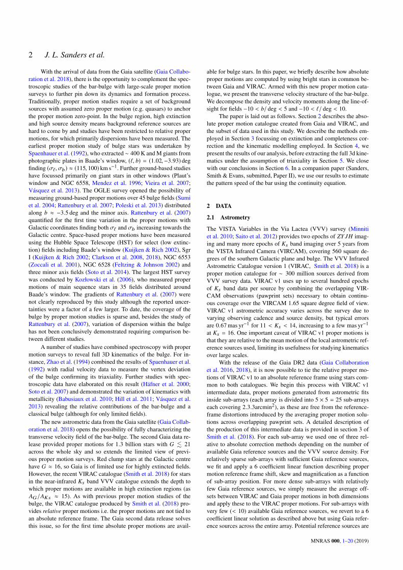
We have simulated our selection using Galaxia (v0.7.2,Sharma et al. 2011) with the default set of parameters. In Fig. 2,we display the colour-magnitude diagrams from VVV and Galaxiafor a 0.04 deg2 field at (`, b) = (−3,−3) deg. Brighter than Ks0 =14.5 deg, there are both giants primarily located in the centre of theGalaxy and foreground blue main sequence stars. The colour cutefficiently removes these. A caveat is that we select stars that don’thave J magnitudes. Some of these stars could be blue main se-quence. However, for our test field the probability of this is at most∼ 1242/8876 ≈ 14 percent, but given a lack of J measurement itis more likely to be a redder star so the probability is significantlylower.

Within the giant selection box, there are nearby lower mainsequence stars but these are subdominant. From Galaxia, we find94/8211 ≈ 1 percent and in the data the cut on parallax removes139 of 8876. The similar ratios give us confidence we are removing

MNRAS 000, 1–20 (2019)

4 J. L. Sanders et al.

Figure 2. Unextincted colour-magnitude diagrams for VVV (left) andGalaxia (right) for a field centred on (`, b) = (−3, −3) deg. Our selectioncorresponds to the top right box. The insets give the number of stars in eachbox and d is the number of dwarfs in the top right box.

most contaminating dwarfs with the parallax cut. At higher lati-tudes, b = −10 deg the dwarf contamination fraction increases to∼ 17 percent but checking with Galaxia, many of these dwarfs arewithin ∼ 1.5 kpc. Removing these reduces the dwarf contamina-tion fraction to 5 percent. Near the plane, fewer Gaia parallaxes areavailable but the dwarf contamination is less of an issue as we areoverwhelmed by the distant giants.

From Galaxia, we find that approximately a third of the se-lected giant stars are from the ‘disc’ populations i.e. they are drawnfrom the disc density profiles as opposed to the bulge profile. Asthe disc density profile is broad compared with the bulge profile,it produces a more featureless magnitude distribution. From purelyphotometric data, it is very difficult to separate these populationsso from the perspective of our modelling both populations togethercomprise the bulge.

For sources observed by both Gaia and VVV, we combine theequatorial proper motions from VIRAC and Gaia DR2 using in-verse variance weighting. This assumes the estimates are indepen-dent which is not completely true due to our absolute-to-relativecorrection procedure for the VIRAC proper motions. We transformthe resulting proper motions to Galactic coordinates propagatingthe covariances. When modelling the proper motions, we adopt thefurther quality cuts:

• σµi < 1.5 mas yr−1.• |µi − 〈µi〉| < 3∆µi .

For component i, σµi is the proper motion uncertainty, 〈µi〉 the me-dian proper motion in a given field and∆µi the dispersion computedusing the 16th and 84th percentile. These two quality cuts remove

spurious proper motions (Smith et al. 2018) as well as those whichare highly uncertain offering little constraining power. Although theproper motion error is a function of Ks , so cutting on proper mo-tion error preferentially removes fainter stars, our modelling willconstrain p(µ|Ks) so this isn’t a concern.

3 METHODOLOGY

Our aim is to deconvolve the volume density and velocity structurefor the data described in Section 2. We approach this problem intwo stages: first, extracting the density structure in small on-skybins by modelling the unextincted Ks magnitude distribution forred giant stars, and secondly, combining the density structure withthe proper motions to extract the transverse velocity distributionsalong the line-of-sight. Before embarking on this, we must modelthe extinction and completeness which are significant for many ofthe considered bulge fields. We then describe the entire kinematicmodel before explaining how it is broken into two stages.

3.1 Extinction

We follow Gonzalez et al. (2011) constructing a 2D extinctionE(J − Ks) from the red clump giant stars (we ignore any extinc-tion variation along the line-of-sight assuming the majority of theextinction is from foreground dust). We divide the VIRAC cata-logue into fields of 3, 5 and 10 arcmin square for |b| < 1.5 deg,1.5 deg < |b| < 5 deg and b < −5 deg. In each field, we select starsin a diagonal colour-magnitude box to account for extinction suchthat J < 14 + 0.482(J − Ks − 0.62) and (J − Ks) > 0.5 and requireuncertainties in J and Ks less than 0.2 mag. In (J −Ks), we find thepeak (J−Ks)RC using a multi-Gaussian fit and record the full-widthhalf-maximum (FWHM) of this peak converting this into a standarddeviation σ(J−Ks). The unextincted red clump in Baade’s windowis (J − Ks)0,BW = 0.62 mag (Simion et al. 2017, obtained by trans-forming the Gonzalez et al. (2011) result to the VVV bands) whichwe assume is valid across the bulge. In each field the extinction isgiven by E(J−Ks) = (J−Ks)RC−(J−Ks)0,BW with correspondinguncertainty σE(J−Ks ) as (Wegg & Gerhard 2013)

σ2E(J−Ks ) = σ(J − Ks)2 − 〈σJ 〉2 − 〈σKs〉2 − σ(J − Ks)2RC, (1)

where we adopt an intrinsic red clump width of σ(J − Ks)RC =0.05 mag and compute the median magnitude uncertainty 〈σi〉 ineach field (if σ2

E(J−Ks ) < 0 we set σE(J−Ks ) = 0). We use theNishiyama et al. (2009) extinction law such that AKs = 0.482E(J−Ks). This is similar to the extinction law AKs = 0.428E(J − Ks)derived directly from VVV photometry by Alonso-García et al.(2017) (Wegg & Gerhard 2013, also considered the Cardelli et al.(1989) extinction law and found the resulting large-scale bar-bulgeproperties to be unchanged). The results of our procedure areshown in the left panel of Fig. 3.

3.2 Completeness

There are two sources of incompleteness in our adopted catalogue.The first is incompleteness in the source catalogues used by VIRACand the second is incompleteness due to each source not beingassigned a proper motion. We assess the first of these using themethod of Saito et al. (2012) and Wegg & Gerhard (2013) by in-specting the recovery of fake stars injected into the VVV images.For each bulge field, we choose the image with seeing closest to

MNRAS 000, 1–20 (2019)

Kinematics of the Galactic bar-bulge 5

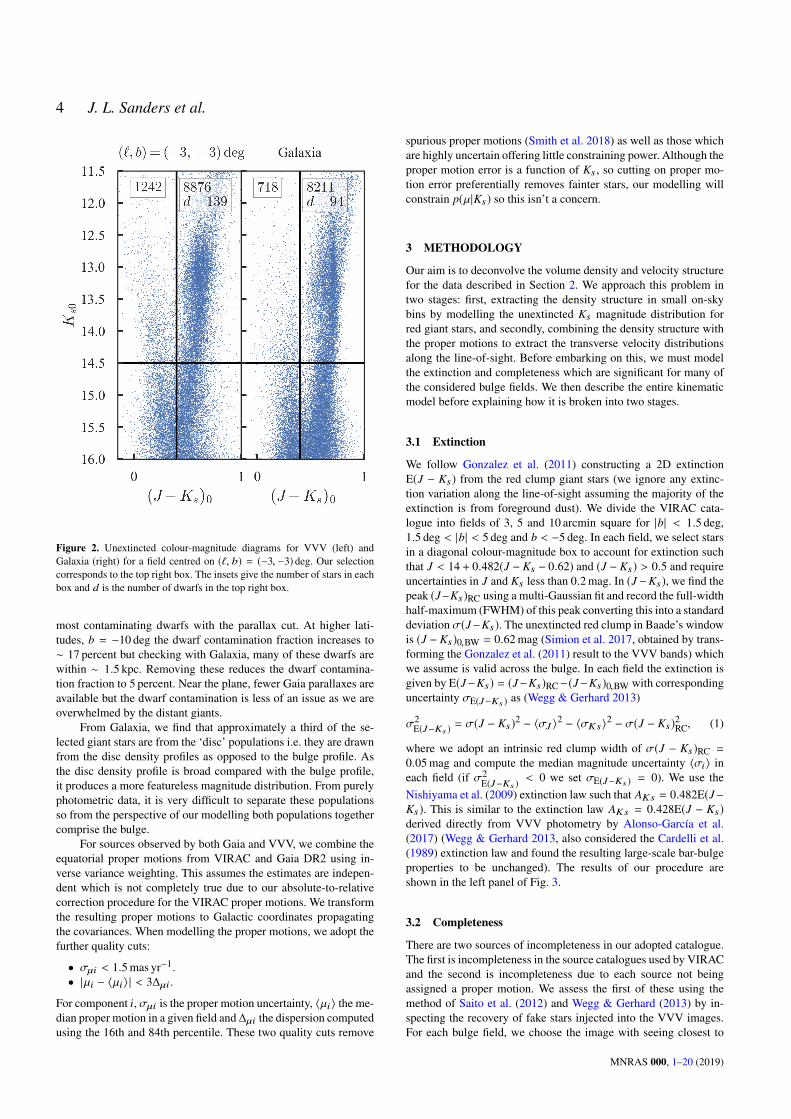
Figure 3. Extinction and completeness: left panel shows the adopted extinction map, central panel the completeness (both source and proper motion complete-ness) at unextincted Ks0 = 14 mag and the right panel shows the completeness at different lines of sight coloured by the Galactic latitude. The three blacklines correspond to the square fields in the central panel.

0.75 arcsec. For each array, we randomly add 5000 stars with ran-domly selected magnitude 11 < Ks < 18 mag (using a Gaussianpsf with FWHM of the seeing) and attempt to extract them usingCASU’s imcore. We repeat this procedure five times and recordthe average fraction extracted as a function of Ks . Naturally thecompleteness correlates with the source density, so is a strong func-tion of b with fields at |b| . 1 deg approximately 50 percent incom-plete at Ks = 16 mag.

Additionally, for each image we compare the true source cat-alogue to the sources with VIRAC proper motions and record thefraction with proper motions as a function of Ks . In general, this in-completeness is less severe than the source incompleteness. Whenanalysing data we are concerned with the incompleteness as afunction of unextincted magnitude. In Fig. 3, we display the totalVIRAC completeness at Ks0 = 14 mag. We see how the complete-ness is a complex function of source density and extinction.

3.3 Kinematic modelling

From the described data, we wish to construct maps of the trans-verse velocity components v` and vb as a function of Galactic lo-cation within the Galactic bulge region. For a single sightline (`, b),we construct p(Ks, µ |Σ), where Ks is the dereddened extinctionKs (we drop the subscript zero from now on), µ = (µ`, µb) is theproper motion vector and

Σ =

(σ2µ`

ρ`bσµ`σµb

ρ`bσµ`σµb σ2µb

)(2)

is the uncertainty covariance matrix with σµi the uncertainty in µiand ρ`b the correlation coefficient. We ignore uncertainties in Ks .This is given by

p(Ks, µ |Σ) = N−1S(Ks)M(Ks, µ |Σ), (3)

where M(Ks, µ |Σ) is the model for the bulge giant stars, S(Ks) isthe completeness ratio and N is a normalization constant given by

N =∫ 14.5

11.5dKs S(Ks)

∫d2µ M(Ks, µ |Σ). (4)

We write

M(Ks, µ |Σ) =∫

ds s2ρ(s)p(MKs)p(µ |MKs, s,Σ), (5)

where ρ(s) is the density profile as a function of distance s along theline-of-sight specified by (`, b). The giant branch luminosity func-tion p(MKs) is evaluated at MKs = Ks − 2.171 ln s − 10 (s in kpc).

The kinematic distribution p(µ |MKs, s,Σ) is in general a functionof location s and stellar type MKs . The kinematics are expected tobe functions of both age and metallicity of the population. How-ever, they will be weak functions of MKs as along the giant branchwe expect all stellar populations to contribute. Therefore, for sim-plicity we model p(µ |s,Σ) only, for which we assume a Gaussianrandom field

p(µ |s,Σ) = N(µ |m(s),Σm(s) + Σ), (6)

where m(s) is the mean proper motion at each distance and Σm(s)the covariance1. We model the density profile using a set of log-Gaussian basis functions.

ρ(s) =Nc∑i

wiN(ln s |gi, σi), (7)

where gi are the set of means in ln s, σi a set of widths, w is asimplex and Nc the number of components which we set to three.

3.4 Luminosity function

Our model is for all giant stars towards the Galactic centre whichcan include both ‘disc’ and ‘bulge’ stars. In theory, we require dif-ferent luminosity functions for each component. However, as thedisc density profile is broad, details of its luminosity function (e.g.metallicity) are unimportant so we use a single luminosity functionfor both components.

The luminosity function p(MKs) is adopted from Simionet al. (2017) composed of three Gaussian peaks for the AGB,RGB and RC bumps along with a background RGB exponen-tial: MKs ∝ exp(ag(MKs + 1.53)) where Simion et al. (2017)sets ag = ag0 = 0.642. Simion et al. (2017) allowed the meanmagnitude of the red clump to vary in their modelling. Requir-ing a Galactic centre distance of 8 kpc, Simion et al. (2017) foundMK,RC = −1.63 mag consistent with the solar neighbourhood re-sult of MK,RC = −1.61 mag (Alves 2000; Hawkins et al. 2017).From stellar models (Girardi & Salaris 2001; Salaris & Girardi2002), the red clump magnitude is a function of (at least) alpha-enhancement, age and metallicity. From different assumptions,Wegg & Gerhard (2013) employed a brighter red clump magnitude

1 Throughout the paper we use the notation N(m, s) for a univariate nor-mal distribution with mean m and standard deviation s and N(m, Σ) for amultivariate normal distribution with mean m and covariance Σ.

MNRAS 000, 1–20 (2019)

6 J. L. Sanders et al.

12 13 14K0

0.0

0.2

0.4

0.6

p(K

0)

Model

Completeness-corrected Raw

6 8 10 12s/kpc

8

6

4

2

0

2

µ/m

asyr−

1

6 8 10 12s/kpc

200

100

0

100

200

v gc/km

s−1

10 0 10µi/mas/yr−1

6 8 10 12s/kpc

0.1

0.2

0.3

ρ(s

)/A

rbitra

ryunits

6 8 10 12s/kpc

0

1

2

3

4

σµ/m

asyr−

1

6 8 10 12s/kpc

0

50

100

150

σ/km

s−1

` b

10 0µ`/mas/yr−1

µb/m

as/yr−

1

ρ= 0.06± 0.01

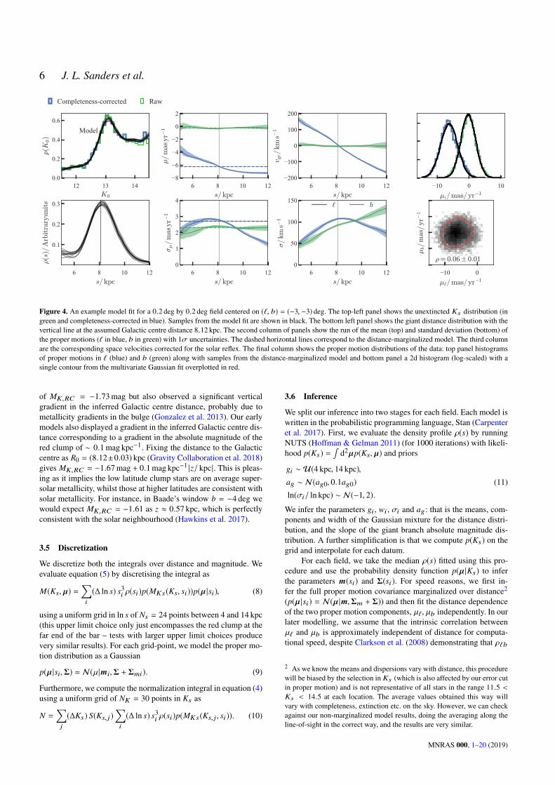
Figure 4. An example model fit for a 0.2 deg by 0.2 deg field centered on (`, b) = (−3, −3) deg. The top-left panel shows the unextincted Ks distribution (ingreen and completeness-corrected in blue). Samples from the model fit are shown in black. The bottom left panel shows the giant distance distribution with thevertical line at the assumed Galactic centre distance 8.12 kpc. The second column of panels show the run of the mean (top) and standard deviation (bottom) ofthe proper motions (` in blue, b in green) with 1σ uncertainties. The dashed horizontal lines correspond to the distance-marginalized model. The third columnare the corresponding space velocities corrected for the solar reflex. The final column shows the proper motion distributions of the data: top panel histogramsof proper motions in ` (blue) and b (green) along with samples from the distance-marginalized model and bottom panel a 2d histogram (log-scaled) with asingle contour from the multivariate Gaussian fit overplotted in red.

of MK,RC = −1.73 mag but also observed a significant verticalgradient in the inferred Galactic centre distance, probably due tometallicity gradients in the bulge (Gonzalez et al. 2013). Our earlymodels also displayed a gradient in the inferred Galactic centre dis-tance corresponding to a gradient in the absolute magnitude of thered clump of ∼ 0.1 mag kpc−1. Fixing the distance to the Galacticcentre as R0 = (8.12±0.03) kpc (Gravity Collaboration et al. 2018)gives MK,RC = −1.67 mag + 0.1 mag kpc−1 |z/ kpc|. This is pleas-ing as it implies the low latitude clump stars are on average super-solar metallicity, whilst those at higher latitudes are consistent withsolar metallicity. For instance, in Baade’s window b = −4 deg wewould expect MK,RC = −1.61 as z ≈ 0.57 kpc, which is perfectlyconsistent with the solar neighbourhood (Hawkins et al. 2017).

3.5 Discretization

We discretize both the integrals over distance and magnitude. Weevaluate equation (5) by discretising the integral as

M(Ks, µ) =∑i

(∆ ln s) s3i ρ(si)p(MKs(Ks, si))p(µ |si), (8)

using a uniform grid in ln s of Ns = 24 points between 4 and 14 kpc(this upper limit choice only just encompasses the red clump at thefar end of the bar – tests with larger upper limit choices producevery similar results). For each grid-point, we model the proper mo-tion distribution as a Gaussian

p(µ |si,Σ) = N(µ|mi,Σ + Σmi). (9)

Furthermore, we compute the normalization integral in equation (4)using a uniform grid of NK = 30 points in Ks as

N =∑j

(∆Ks) S(Ks, j )∑i

(∆ ln s) s3i ρ(si)p(MKs(Ks, j, si)). (10)

3.6 Inference

We split our inference into two stages for each field. Each model iswritten in the probabilistic programming language, Stan (Carpenteret al. 2017). First, we evaluate the density profile ρ(s) by runningNUTS (Hoffman & Gelman 2011) (for 1000 iterations) with likeli-hood p(Ks) =

∫d2µp(Ks, µ) and priors

gi ∼ U(4 kpc, 14 kpc),ag ∼ N(ag0, 0.1ag0)ln(σi/ ln kpc) ∼ N(−1, 2).

(11)

We infer the parameters gi , wi , σi and ag: that is the means, com-ponents and width of the Gaussian mixture for the distance distri-bution, and the slope of the giant branch absolute magnitude dis-tribution. A further simplification is that we compute p(Ks) on thegrid and interpolate for each datum.

For each field, we take the median ρ(s) fitted using this pro-cedure and use the probability density function p(µ |Ks) to inferthe parameters m(si) and Σ(si). For speed reasons, we first in-fer the full proper motion covariance marginalized over distance2

(p(µ |si) = N(µ |m,Σm + Σ)) and then fit the distance dependenceof the two proper motion components, µ`, µb independently. In ourlater modelling, we assume that the intrinsic correlation betweenµ` and µb is approximately independent of distance for computa-tional speed, despite Clarkson et al. (2008) demonstrating that ρ`b

2 As we know the means and dispersions vary with distance, this procedurewill be biased by the selection in Ks (which is also affected by our error cutin proper motion) and is not representative of all stars in the range 11.5 <Ks < 14.5 at each location. The average values obtained this way willvary with completeness, extinction etc. on the sky. However, we can checkagainst our non-marginalized model results, doing the averaging along theline-of-sight in the correct way, and the results are very similar.

MNRAS 000, 1–20 (2019)

Kinematics of the Galactic bar-bulge 7

varies with distance within the bulge. For each model, we run theNUTS sampler for 100 iterations. We work with proper motions,µ′, shifted by the median and scaled by the standard deviation. Weadopt a ‘smoothing spline’ prior to regularize p(µ′ |s) as

m′i si ∼ N(2m′i−1si−1 − m′i−2si−2, τm(8 kpc)),σ′i si ∼ N(2σ

′i−1si−1 − σ

′i−2si−2, τs(8 kpc)),

(12)

where m′i and σ′i are the mean and variance for a single scaled andshifted proper motion component at distance si . These priors actto minimize the second derivatives with respect to log-distance ofthe mean and standard deviations of the physical velocities (hencemultiplying by the distance). We further adopt the priors

m′1 ∼ N(0, 5), m′2 ∼ N(0, 5), τm ∼ N(0, 1), τm > 0,σ′1 ∼ N(0, 5), σ

′2 ∼ N(0, 5), τs ∼ N(0, 1), τs > 0.

(13)

For the distance-marginalized model, we adopt

m′ ∼ N(0, 5), σ′ ∼ N(1, 5), ρ`b ∼ N(0, 0.4), (14)

where ρ`b is the covariance. In principle, we could also imposesmoothing in the means and dispersions between different (`, b)pixels. However, such a model would have a very large numberof free parameters, so we analyse each field independently.

Transverse velocities are estimated in the heliocentric framewhich we transform to the Galactocentric frame using a solar mo-tion of (U,V + Vc,W) = (11.1, 245.5, 7.25) km s−1 (Reid & Brun-thaler 2004; Gravity Collaboration et al. 2018; Schönrich et al.2010).

3.7 An example field

In Figure 4, we show the results of fitting the model to a 0.2 deg by0.2 deg field at (`, b) = (−3,−3) deg. This field has 9203 stars sat-isfying our initial set of cuts and 8945/8952 satisfying the propermotion cuts in `/b. The first column of panels shows the resultsof the density fit. Both the raw and the completeness-correctedunextincted magnitude distributions are displayed along with ourmodel fit. The peak of the bulge red giants is clearly visible atK0 ∼ 13 mag. This corresponds to the inferred density distributionin the lower panel peaking just beyond the assumed Galactic Cen-tre distance. The second column shows the inferred run of the meanand standard deviation of the proper motions in the two componentsalong with uncertainties. We also show the average inferred frommarginalization over distance. The third column shows the corre-sponding solar-reflex-corrected velocities. The mean µb and vb areflat implying no net vertical flow at any position (as per expecta-tion). The longitude motion is more interesting. The mean propermotion falls from ∼ −4 mas yr−1 at s = 5 kpc to ∼ −7 mas yr−1

beyond s = 10 kpc. In the velocities, this corresponds to a ‘rotationcurve’ crossing zero near the Galactic centre distance and rising to∼ 150 km s−1 at the extremes. We also note the slight change in gra-dient ∼ 1 kpc from the Galactic centre which mirrors the rotationcurves derived from proper motion data by Clarkson et al. (2008).

The velocity dispersions rise from (σ`, σb) ≈ (50, 50) km s−1

at s = 5 kpc towards the Galactic centre distance. σ` peaks at theGalactic centre at ∼ 105 km s−1 and declines to ∼ 70 km s−1 ats = 12 kpc whilst σb continues to rise. The σb behaviour is not ex-actly in agreement with our expectations. It appears that the modelstruggles to distinguish between stars at the Galactic centre andthose beyond it, assigning a similar proper motion dispersion toboth populations. The problem is not mirrored in ` possibly be-cause the mean is evolving. We have inspected the µb distribution

10.07.55.02.50.02.55.07.510.0`/deg

10

8

6

4

2

0

2

4

b/deg

N= 44374158, Nc− c = 58950234

0 5000

1000

0

1500

0

2000

0

2500

0

Ngiants

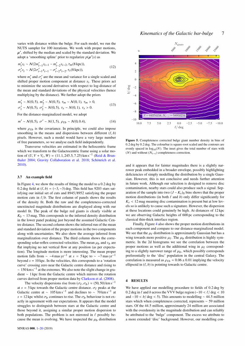
Figure 5. Completeness corrected bulge giant number density in bins of0.2 deg by 0.2 deg. The colourbar is square-root scaled and the contours areevenly spaced in log10(N ). The inset gives the total number of stars with(N ) and without (Nc−c) completeness correction.

and it appears that for fainter magnitudes there is a slightly nar-rower peak embedded in a broader envelope, possibly highlightingdeficiencies of simply modelling the distribution by a single Gaus-sian. However, this is not conclusive and needs further attentionin future work. Although our selection is designed to remove disccontamination, nearby stars could also produce such a signal. Sep-aration of the sample into two (J − Ks)0 bins shows that the propermotion distributions (in both ` and b) only differ significantly forKs < 12 mag meaning disc contamination is present but at low lev-els so is unlikely to cause such a signature. However, the dispersionat these locations could genuinely be high. At distances of 12 kpcwe are observing Galactic heights of 600 pc corresponding to theclassical thin-thick interface region.

Finally, Figure 4 also shows the proper motion distributions ineach component and compare to our distance-marginalized model.We see that the µ` distribution is approximately Gaussian but has awing towards more positive µ` . The µb distribution is highly sym-metric. In the 2d histograms we see the correlation between theproper motions as well as the additional wing in µ` correspond-ing to a slightly narrower range of µb , which possibly correspondspreferentially to the ‘disc’ population in the central Galaxy. Thecorrelation is measured as ρ`b = 0.06± 0.01 implying the velocityellipsoid in (`, b) is pointing towards to Galactic centre.

4 RESULTS

We have applied our modelling procedure to fields of 0.2 deg by0.2 deg in ` and b across the VVV bulge region (−10 < `/ deg < 10and −10 < b/ deg < 5). This amounts to modelling ∼ 44.5 millionstars which when completeness corrected, represents ∼ 59 millionstars. Of the 44.5 million, approximately 24 million are associatedwith the overdensity in the magnitude distribution and can reliablybe attributed to the ‘bulge’ component. The excess we attribute toa more extended ‘disc’ background. However, our modelling con-

MNRAS 000, 1–20 (2019)

8 J. L. Sanders et al.

1050510`/deg

10

8

6

4

2

0

2

4

b/deg

Total dispersions

1050510`/deg

10

8

6

4

2

0

2

4

b/deg

Line-of-sight averaged dispersions

1050510`/deg

10

8

6

4

2

0

2

4

b/deg

1050510`/deg

10

8

6

4

2

0

2

4

b/deg

1050510`/deg

10

8

6

4

2

0

2

4

b/deg

1050510`/deg

10

8

6

4

2

0

2

4

b/deg

1.8 2.0 2.2 2.4 2.6 2.8 3.0

⟨σ`⟩/masyr−1

2.0 2.2 2.4 2.6 2.8 3.0 3.2

σ`/masyr−1

1.8 2.0 2.2 2.4 2.6 2.8 3.0

⟨σb⟩/masyr−1

1.8 2.0 2.2 2.4 2.6 2.8 3.0

σb/masyr−10.9

0

0.95

1.00

1.05

1.10

1.15

1.20

1.25

1.30

Dispersion ratio ⟨σ`⟩/⟨σb⟩

1.0 1.1 1.2 1.3 1.4 1.5

Dispersion ratio σ`/σb

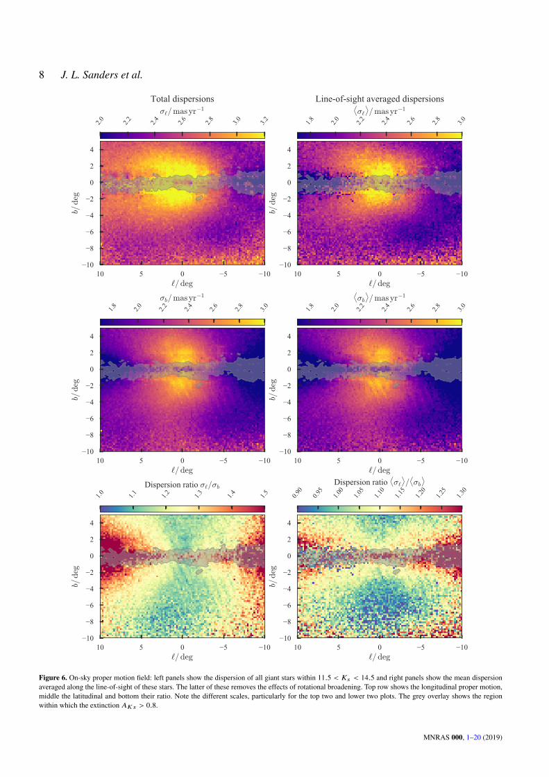
Figure 6. On-sky proper motion field: left panels show the dispersion of all giant stars within 11.5 < Ks < 14.5 and right panels show the mean dispersionaveraged along the line-of-sight of these stars. The latter of these removes the effects of rotational broadening. Top row shows the longitudinal proper motion,middle the latitudinal and bottom their ratio. Note the different scales, particularly for the top two and lower two plots. The grey overlay shows the regionwithin which the extinction AKs > 0.8.

MNRAS 000, 1–20 (2019)

Kinematics of the Galactic bar-bulge 9

10.07.55.02.50.02.55.07.510.0`/deg

10

8

6

4

2

0

2

4

b/deg

Median error ~ 0.017

0.15

0.10

0.05

0.00

0.05

0.10

0.15

Correlation between µ` and µb

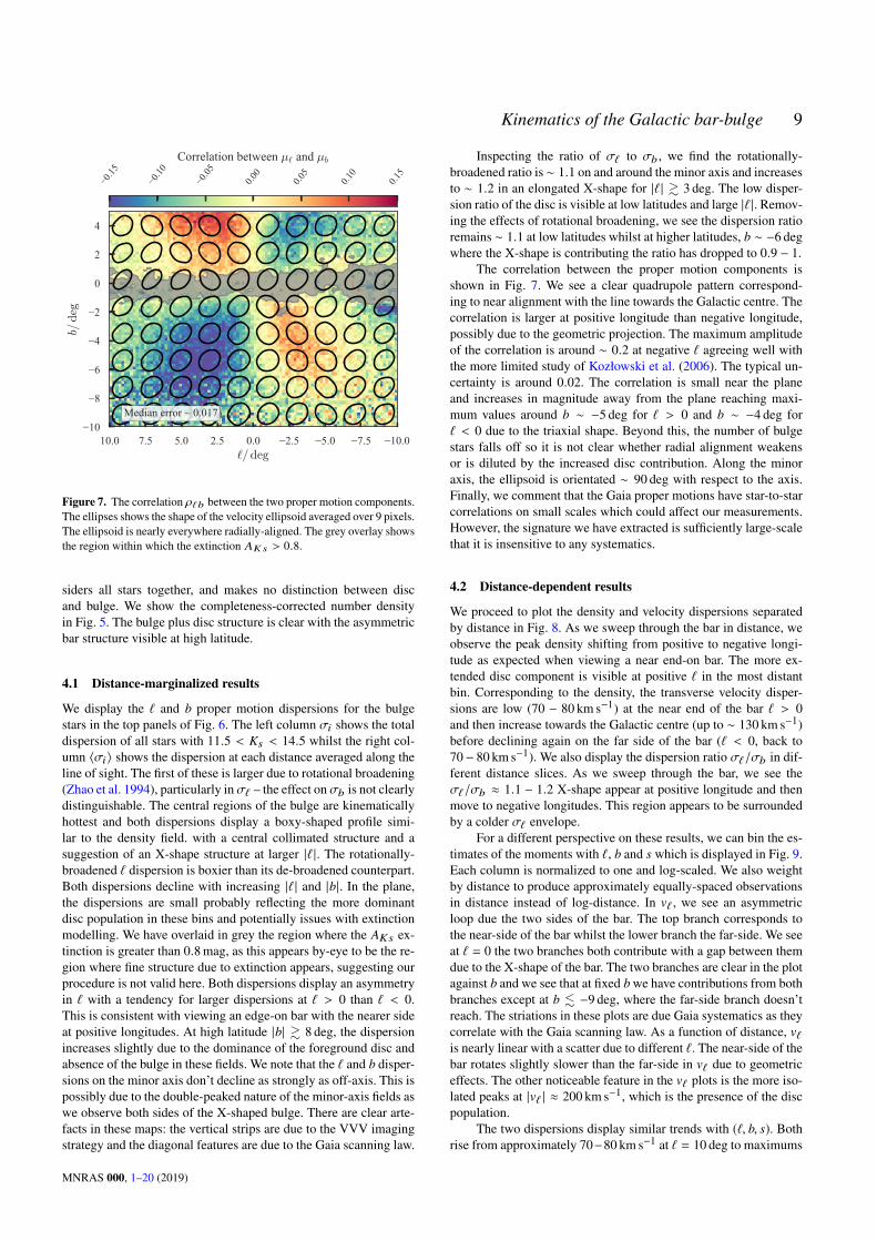
Figure 7. The correlation ρ`b between the two proper motion components.The ellipses shows the shape of the velocity ellipsoid averaged over 9 pixels.The ellipsoid is nearly everywhere radially-aligned. The grey overlay showsthe region within which the extinction AKs > 0.8.

siders all stars together, and makes no distinction between discand bulge. We show the completeness-corrected number densityin Fig. 5. The bulge plus disc structure is clear with the asymmetricbar structure visible at high latitude.

4.1 Distance-marginalized results

We display the ` and b proper motion dispersions for the bulgestars in the top panels of Fig. 6. The left column σi shows the totaldispersion of all stars with 11.5 < Ks < 14.5 whilst the right col-umn 〈σi〉 shows the dispersion at each distance averaged along theline of sight. The first of these is larger due to rotational broadening(Zhao et al. 1994), particularly in σ` – the effect on σb is not clearlydistinguishable. The central regions of the bulge are kinematicallyhottest and both dispersions display a boxy-shaped profile simi-lar to the density field. with a central collimated structure and asuggestion of an X-shape structure at larger |` |. The rotationally-broadened ` dispersion is boxier than its de-broadened counterpart.Both dispersions decline with increasing |` | and |b|. In the plane,the dispersions are small probably reflecting the more dominantdisc population in these bins and potentially issues with extinctionmodelling. We have overlaid in grey the region where the AKs ex-tinction is greater than 0.8 mag, as this appears by-eye to be the re-gion where fine structure due to extinction appears, suggesting ourprocedure is not valid here. Both dispersions display an asymmetryin ` with a tendency for larger dispersions at ` > 0 than ` < 0.This is consistent with viewing an edge-on bar with the nearer sideat positive longitudes. At high latitude |b| & 8 deg, the dispersionincreases slightly due to the dominance of the foreground disc andabsence of the bulge in these fields. We note that the ` and b disper-sions on the minor axis don’t decline as strongly as off-axis. This ispossibly due to the double-peaked nature of the minor-axis fields aswe observe both sides of the X-shaped bulge. There are clear arte-facts in these maps: the vertical strips are due to the VVV imagingstrategy and the diagonal features are due to the Gaia scanning law.

Inspecting the ratio of σ` to σb , we find the rotationally-broadened ratio is ∼ 1.1 on and around the minor axis and increasesto ∼ 1.2 in an elongated X-shape for |` | & 3 deg. The low disper-sion ratio of the disc is visible at low latitudes and large |` |. Remov-ing the effects of rotational broadening, we see the dispersion ratioremains ∼ 1.1 at low latitudes whilst at higher latitudes, b ∼ −6 degwhere the X-shape is contributing the ratio has dropped to 0.9 − 1.

The correlation between the proper motion components isshown in Fig. 7. We see a clear quadrupole pattern correspond-ing to near alignment with the line towards the Galactic centre. Thecorrelation is larger at positive longitude than negative longitude,possibly due to the geometric projection. The maximum amplitudeof the correlation is around ∼ 0.2 at negative ` agreeing well withthe more limited study of Kozłowski et al. (2006). The typical un-certainty is around 0.02. The correlation is small near the planeand increases in magnitude away from the plane reaching maxi-mum values around b ∼ −5 deg for ` > 0 and b ∼ −4 deg for` < 0 due to the triaxial shape. Beyond this, the number of bulgestars falls off so it is not clear whether radial alignment weakensor is diluted by the increased disc contribution. Along the minoraxis, the ellipsoid is orientated ∼ 90 deg with respect to the axis.Finally, we comment that the Gaia proper motions have star-to-starcorrelations on small scales which could affect our measurements.However, the signature we have extracted is sufficiently large-scalethat it is insensitive to any systematics.

4.2 Distance-dependent results

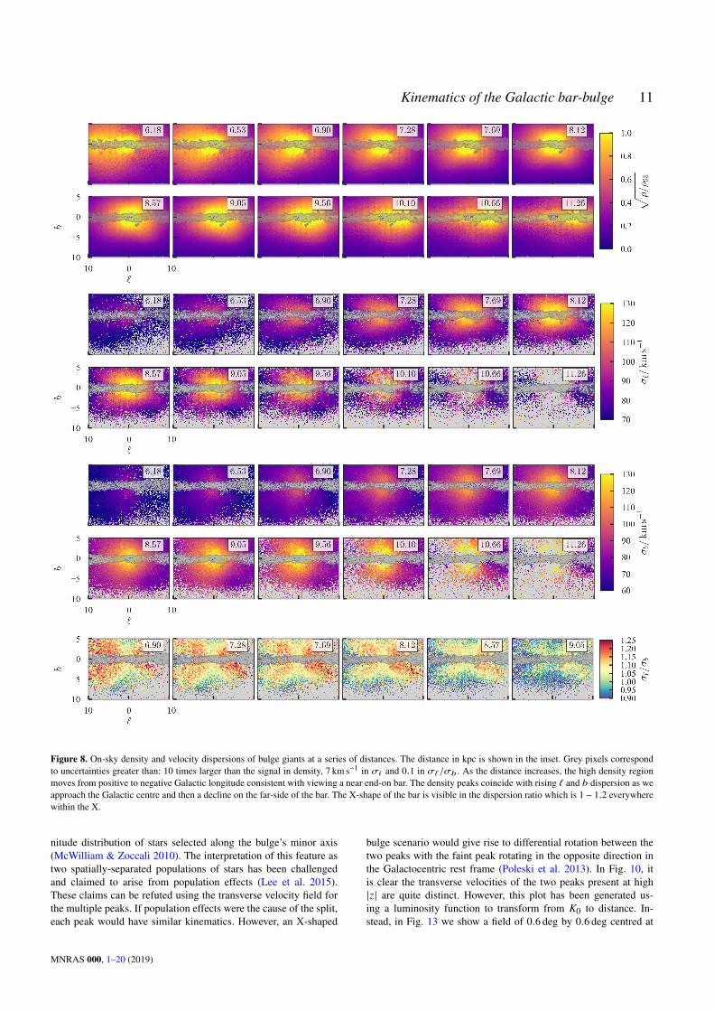
We proceed to plot the density and velocity dispersions separatedby distance in Fig. 8. As we sweep through the bar in distance, weobserve the peak density shifting from positive to negative longi-tude as expected when viewing a near end-on bar. The more ex-tended disc component is visible at positive ` in the most distantbin. Corresponding to the density, the transverse velocity disper-sions are low (70 − 80 km s−1) at the near end of the bar ` > 0and then increase towards the Galactic centre (up to ∼ 130 km s−1)before declining again on the far side of the bar (` < 0, back to70− 80 km s−1). We also display the dispersion ratio σ`/σb in dif-ferent distance slices. As we sweep through the bar, we see theσ`/σb ≈ 1.1 − 1.2 X-shape appear at positive longitude and thenmove to negative longitudes. This region appears to be surroundedby a colder σ` envelope.

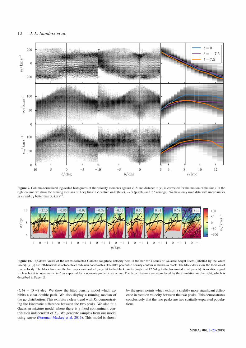
For a different perspective on these results, we can bin the es-timates of the moments with `, b and s which is displayed in Fig. 9.Each column is normalized to one and log-scaled. We also weightby distance to produce approximately equally-spaced observationsin distance instead of log-distance. In v` , we see an asymmetricloop due the two sides of the bar. The top branch corresponds tothe near-side of the bar whilst the lower branch the far-side. We seeat ` = 0 the two branches both contribute with a gap between themdue to the X-shape of the bar. The two branches are clear in the plotagainst b and we see that at fixed b we have contributions from bothbranches except at b . −9 deg, where the far-side branch doesn’treach. The striations in these plots are due Gaia systematics as theycorrelate with the Gaia scanning law. As a function of distance, v`is nearly linear with a scatter due to different `. The near-side of thebar rotates slightly slower than the far-side in v` due to geometriceffects. The other noticeable feature in the v` plots is the more iso-lated peaks at |v` | ≈ 200 km s−1, which is the presence of the discpopulation.

The two dispersions display similar trends with (`, b, s). Bothrise from approximately 70−80 km s−1 at ` = 10 deg to maximums

MNRAS 000, 1–20 (2019)

10 J. L. Sanders et al.

of 100 − 130 km s−1 at ` = 0 declining again towards ` = −10 deg.Both dispersions are weakly asymmetric in ` due to geometric ef-fects. In b, we observe similar but more symmetric behaviour. Thegradients with b are present but significantly flatter than those in`. Noticeably the disc population is visible in the midplane at lowdispersions. Against distance, both profiles rise from ∼ 40 km s−1

towards the Galactic centre. Beyond this, σ` instantly declines backdown to near its near-field value (specifically for ` = 7.5) whilst σbplateaus before declining beyond 10 kpc (a feature also seen in ourexample field in Fig. 4). The coloured lines show the averages over1 deg bins in `. We see that the dispersion for the near-side of thebar ` > 0 peaks at smaller distances than the far-side ` < 0.

We can compare the dispersion profiles with those obtainedfor disc stars in e.g. Sanders & Das (2018). The run of vertical dis-persion σb appears to connect onto the vertical dispersion with ra-dius presented there although for the intermediate-age populations.This might be a reflection of selection effects of our approach (e.g.red clump stars are more likely from a younger population ∼ 2 Gyr)but perhaps more interestingly could be a reflection of the popula-tions within the bar and when the bar buckled.

In Fig. 10, we display the v` field in Galactocentric Cartesiancoordinates at a range of z slices. We see a clear asymmetry in thevelocity field indicative of the bar (an axisymmetric rotation fieldin this space would be symmetric ±y). We find that in all z slices,the line-of-nodes (where v` = 0) is orientated at ∼ 77.5 deg to` = 0. We display a plot for results from a simulation (describedin Paper II) which shows a similar relationship between the major-axis of the bar and the line-of-nodes in v` . We also observe at highlatitude (e.g. z = 860 pc) the double peaked density field is visibleand corresponds to distinctly different kinematics.

4.3 Comparison with previous studies

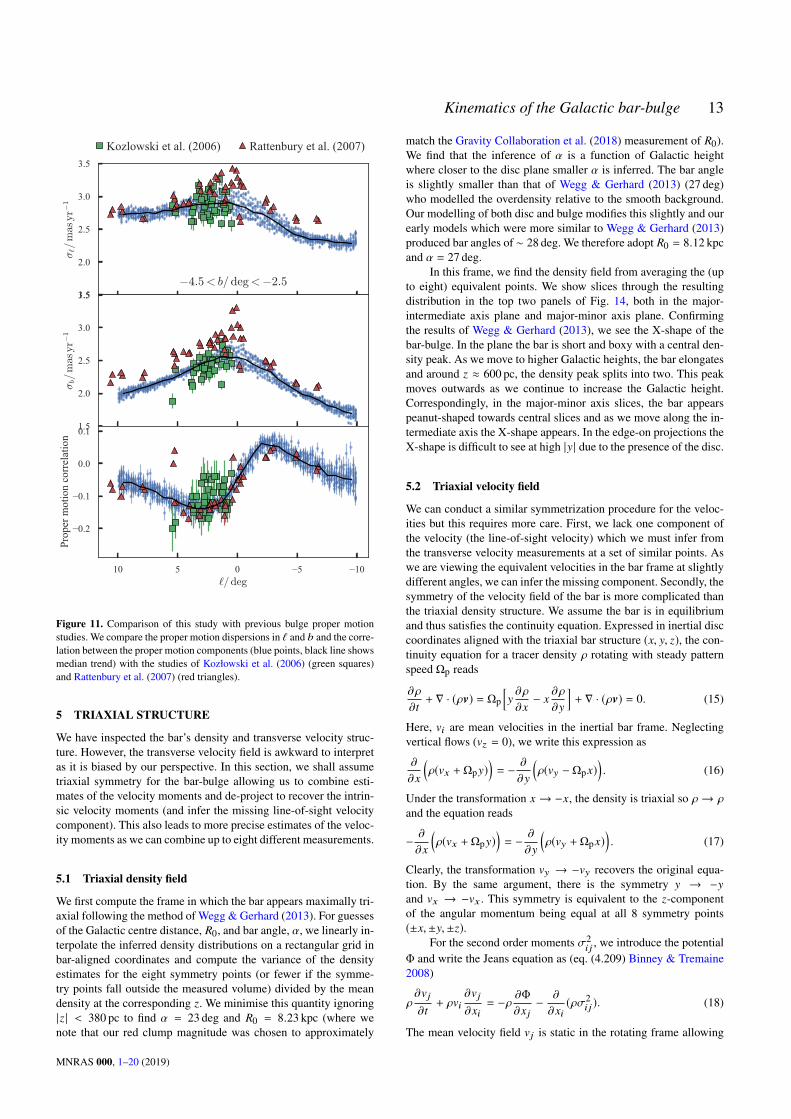
Early proper motion studies of the bulge were restricted to anumber of isolated low-extinction fields (Spaenhauer et al. 1992;Mendez et al. 1996; Zoccali et al. 2001; Kuijken & Rich 2002;Feltzing & Johnson 2002). Additionally, the lack of backgroundsources restricted these studies to relative proper motions and henceno measurement of the mean transverse velocities. The large HSTprogramme of Kozłowski et al. (2006) extended the coverage ofthe bulge proper motions to 35 fields centred around (`, b) =(2.5,−3) deg for 16.5 < I < 21.5 and Rattenbury et al. (2007) usedthe OGLE proper motion catalogue of Sumi et al. (2004) for 45fields distributed mainly along b ≈ −3.5 deg for 12.5 < I < 14.5.Both authors measured the proper motion dispersions and the cor-relation between the components of the proper motion. Both stud-ies produced consistent results finding a declining σb profile with `and variation of the proper motion correlation across the inspectedfields. In Fig. 11, we show a comparison of our proper motion mea-surements (not removing rotational broadening effects) within theslice −4.5 < b/ deg < −2.5 with those of Kozłowski et al. (2006)and Rattenbury et al. (2007). For the Rattenbury et al. (2007) mea-surements, the random errorbars are typically smaller than the dat-apoints (∼ 0.02 mas yr−1). Our σ` measurements agree well withthose of Kozłowski et al. (2006) and are smaller than those of Rat-tenbury et al. (2007). On the whole, we find very good agreementbetween our measurements and these previous studies. As we moveaway from the minor axis, our measurements decline with the fallin σb steeper than that in σ` . In both dispersions, there is asym-metry in ` with lower dispersions on the far-side of the bar. Ourmeasurements are consistent with Kozłowski et al. (2006) and gen-erally slightly smaller than Rattenbury et al. (2007), except in σ`

for ` > 0. This agrees with the models of Portail et al. (2017),who found the Rattenbury et al. (2007) dispersions overpredict theirmodel (their figure 16). This discrepancy could be causd by under-estimated uncertainties in Rattenbury et al. (2007) or by the pres-ence of contaminating populations.

Finally, the correlation measurements agree well with bothprevious studies over the entire ` range, in particular with the Rat-tenbury et al. (2007) results. As observed previously, the corre-lation is smaller at negative longitude than at positive longitude.In the range 0 < `/ deg < 5 our measured correlation is smaller(greater magnitude) than some of the Kozłowski et al. (2006) mea-surements.

4.4 Comparison with spectroscopic surveys

With proper motions, only two components of the velocity field canbe mapped, unless we enforce some symmetry as in Section 5. Tofully map the velocity field, we require results from spectroscopicsurveys. Whilst we reserve the combination of spectroscopic obser-vations with the proper motions provided here to a separate work,we here briefly compare the transverse velocity measurements tothe line-of-sight measurements across the bulge.

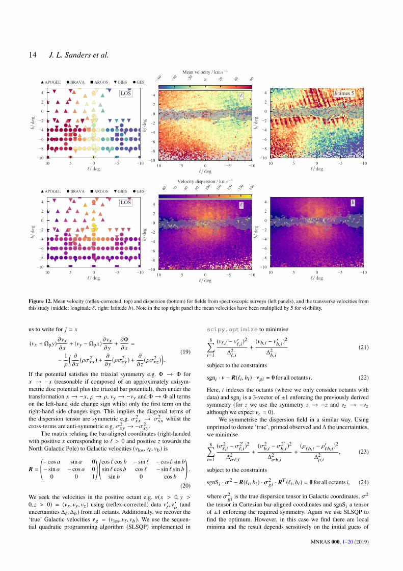
We consider results from five spectroscopic surveys: BRAVA,ARGOS, APOGEE, GIBS and Gaia-ESO. For BRAVA and AR-GOS, we take the mean velocities and dispersions from Kunderet al. (2012) and Ness et al. (2013b) using our assumed solar ve-locities. For APOGEE, we take all fields from DR14 (Abolfathiet al. 2018) within the VVV bulge footprint, remove duplicates anddwarf stars (log g > 3.5) and compute the mean velocity (correctedfor the solar reflex) and dispersion in each field. For Gaia-ESO,we adopt a similar procedure using DR3 (Gilmore et al. 2012).There is only a single field with a sufficient number of stars (at(`, b) ∼ (1,−4) deg). We remove dwarf stars if log g is availableand apply a parallax cut of $ < 1.5 mas to remove nearby con-taminants. For GIBS we use the radial velocity data from Zoccaliet al. (2014) and compute the reflex-corrected mean velocity anddispersion in each of the 33 fields.

In Fig. 12, we compare the line-of-sight mean velocities anddispersions from these surveys with the results from this paper forthe transverse velocity field. To attempt to compare like-to-like,we have averaged the derived transverse velocities weighted by thedensity profile along the line-of-sight. In the mean velocities, thereis a rotation signature in all three components. The strongest sig-nature is in the line-of-sight velocities. The longitudinal rotationsignature is weaker but still visible, particularly for ` > 0 wherethe rotation is increasingly in the longitudinal direction. The rota-tion signature is also visible in the latitudinal direction, where aswe move away from the plane there is a small rotation projection inthis direction. The anticipated quadrupole signature is offset fromthe minor axis due to the geometry of the bar. We note that in theseprojections the Gaia scanning law is visible, particularly near theplane for the b velocities.

In the dispersions, we see a consistent lobed structure acrossthe three velocity components with the line-of-sight dispersionlarger than the longitudinal and latitudinal. The line-of-sight andlongitudinal lobes are more flattened and boxy than the slightly col-limated latitudinal lobe.

4.5 The double red clump

One of the key pieces of evidence pointing towards an X-shapedbar-bulge is the presence of a double red clump peak in the mag-

MNRAS 000, 1–20 (2019)

Kinematics of the Galactic bar-bulge 11

Figure 8. On-sky density and velocity dispersions of bulge giants at a series of distances. The distance in kpc is shown in the inset. Grey pixels correspondto uncertainties greater than: 10 times larger than the signal in density, 7 km s−1 in σi and 0.1 in σ`/σb . As the distance increases, the high density regionmoves from positive to negative Galactic longitude consistent with viewing a near end-on bar. The density peaks coincide with rising ` and b dispersion as weapproach the Galactic centre and then a decline on the far-side of the bar. The X-shape of the bar is visible in the dispersion ratio which is 1 − 1.2 everywherewithin the X.

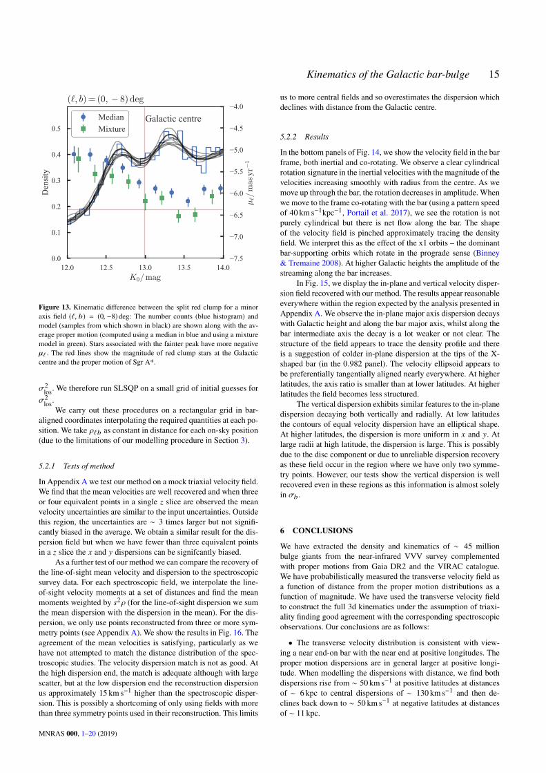
nitude distribution of stars selected along the bulge’s minor axis(McWilliam & Zoccali 2010). The interpretation of this feature astwo spatially-separated populations of stars has been challengedand claimed to arise from population effects (Lee et al. 2015).These claims can be refuted using the transverse velocity field forthe multiple peaks. If population effects were the cause of the split,each peak would have similar kinematics. However, an X-shaped

bulge scenario would give rise to differential rotation between thetwo peaks with the faint peak rotating in the opposite direction inthe Galactocentric rest frame (Poleski et al. 2013). In Fig. 10, itis clear the transverse velocities of the two peaks present at high|z | are quite distinct. However, this plot has been generated us-ing a luminosity function to transform from K0 to distance. In-stead, in Fig. 13 we show a field of 0.6 deg by 0.6 deg centred at

MNRAS 000, 1–20 (2019)

12 J. L. Sanders et al.

200

0

200

v `/km

s−1

`= 0

`= − 7.5

`= 7.5

0

50

100

σ`/km

s−1

1050510`/deg

0

50

100

σb/km

s−1

10 5 0 5b/deg

6 8 10 12s/kpc

Figure 9. Column-normalized log-scaled histograms of the velocity moments against `, b and distance s (v` is corrected for the motion of the Sun). In theright column we show the running medians of 1 deg bins in ` centred on 0 (blue), −7.5 (purple) and 7.5 (orange). We have only used data with uncertaintiesin v` and σi better than 30 km s−1.

101

6

8

10

x/k

pc

−1.10

101

−0.86

101

−0.62

101

−0.38

101y/kpc

−0.14

101

0.10

101

0.34

101

0.58

101

0.82Sim

100

50

0

50

100

v `/km

s−1

Figure 10. Top-down views of the reflex-corrected Galactic longitude velocity field in the bar for a series of Galactic height slices (labelled by the whiteinsets). (x, y) are left-handed Galactocentric Cartesian coordinates. The 80th percentile density contour is shown in black. The black dots show the location ofzero velocity. The black lines are the bar major axis and a by-eye fit to the black points (angled at 12.5 deg to the horizontal in all panels). A rotation signalis clear but it is asymmetric in ` as expected for a non-axisymmetric structure. The broad features are reproduced by the simulation on the right, which isdescribed in Paper II.

(`, b) = (0,−8) deg. We show the fitted density model which ex-hibits a clear double peak. We also display a running median ofthe µ` distribution. This exhibits a clear trend with K0 demonstrat-ing the kinematic difference between the two peaks. We also fit aGaussian mixture model where there is a fixed contaminant con-tribution independent of K0. We generate samples from our modelusing emcee (Foreman-Mackey et al. 2013). This model is shown

by the green points which exhibit a slightly more significant differ-ence in rotation velocity between the two peaks. This demonstratesconclusively that the two peaks are two spatially-separated popula-tions.

MNRAS 000, 1–20 (2019)

Kinematics of the Galactic bar-bulge 13

1.5

2.0

2.5

3.0

3.5

σ`/m

asyr−

1

−4.5<b/deg<−2.5

Kozlowski et al. (2006) Rattenbury et al. (2007)

1.5

2.0

2.5

3.0

3.5

σb/m

asyr−

1

1050510`/deg

0.2

0.1

0.0

0.1

Prop

er m

otio

n co

rrel

atio

n

Figure 11. Comparison of this study with previous bulge proper motionstudies. We compare the proper motion dispersions in ` and b and the corre-lation between the proper motion components (blue points, black line showsmedian trend) with the studies of Kozłowski et al. (2006) (green squares)and Rattenbury et al. (2007) (red triangles).

5 TRIAXIAL STRUCTURE

We have inspected the bar’s density and transverse velocity struc-ture. However, the transverse velocity field is awkward to interpretas it is biased by our perspective. In this section, we shall assumetriaxial symmetry for the bar-bulge allowing us to combine esti-mates of the velocity moments and de-project to recover the intrin-sic velocity moments (and infer the missing line-of-sight velocitycomponent). This also leads to more precise estimates of the veloc-ity moments as we can combine up to eight different measurements.

5.1 Triaxial density field

We first compute the frame in which the bar appears maximally tri-axial following the method of Wegg & Gerhard (2013). For guessesof the Galactic centre distance, R0, and bar angle, α, we linearly in-terpolate the inferred density distributions on a rectangular grid inbar-aligned coordinates and compute the variance of the densityestimates for the eight symmetry points (or fewer if the symme-try points fall outside the measured volume) divided by the meandensity at the corresponding z. We minimise this quantity ignoring|z | < 380 pc to find α = 23 deg and R0 = 8.23 kpc (where wenote that our red clump magnitude was chosen to approximately

match the Gravity Collaboration et al. (2018) measurement of R0).We find that the inference of α is a function of Galactic heightwhere closer to the disc plane smaller α is inferred. The bar angleis slightly smaller than that of Wegg & Gerhard (2013) (27 deg)who modelled the overdensity relative to the smooth background.Our modelling of both disc and bulge modifies this slightly and ourearly models which were more similar to Wegg & Gerhard (2013)produced bar angles of ∼ 28 deg. We therefore adopt R0 = 8.12 kpcand α = 27 deg.

In this frame, we find the density field from averaging the (upto eight) equivalent points. We show slices through the resultingdistribution in the top two panels of Fig. 14, both in the major-intermediate axis plane and major-minor axis plane. Confirmingthe results of Wegg & Gerhard (2013), we see the X-shape of thebar-bulge. In the plane the bar is short and boxy with a central den-sity peak. As we move to higher Galactic heights, the bar elongatesand around z ≈ 600 pc, the density peak splits into two. This peakmoves outwards as we continue to increase the Galactic height.Correspondingly, in the major-minor axis slices, the bar appearspeanut-shaped towards central slices and as we move along the in-termediate axis the X-shape appears. In the edge-on projections theX-shape is difficult to see at high |y | due to the presence of the disc.

5.2 Triaxial velocity field

We can conduct a similar symmetrization procedure for the veloc-ities but this requires more care. First, we lack one component ofthe velocity (the line-of-sight velocity) which we must infer fromthe transverse velocity measurements at a set of similar points. Aswe are viewing the equivalent velocities in the bar frame at slightlydifferent angles, we can infer the missing component. Secondly, thesymmetry of the velocity field of the bar is more complicated thanthe triaxial density structure. We assume the bar is in equilibriumand thus satisfies the continuity equation. Expressed in inertial disccoordinates aligned with the triaxial bar structure (x, y, z), the con-tinuity equation for a tracer density ρ rotating with steady patternspeed Ωp reads

∂ρ

∂t+ ∇ · (ρv) = Ωp

[y∂ρ

∂x− x

∂ρ

∂y

]+ ∇ · (ρv) = 0. (15)

Here, vi are mean velocities in the inertial bar frame. Neglectingvertical flows (vz = 0), we write this expression as

∂

∂x

(ρ(vx +Ωpy)

)= − ∂

∂y

(ρ(vy −Ωpx)

). (16)

Under the transformation x → −x, the density is triaxial so ρ→ ρ

and the equation reads

− ∂

∂x

(ρ(vx +Ωpy)

)= − ∂

∂y

(ρ(vy +Ωpx)

). (17)

Clearly, the transformation vy → −vy recovers the original equa-tion. By the same argument, there is the symmetry y → −yand vx → −vx . This symmetry is equivalent to the z-componentof the angular momentum being equal at all 8 symmetry points(±x,±y,±z).

For the second order moments σ2i j , we introduce the potential

Φ and write the Jeans equation as (eq. (4.209) Binney & Tremaine2008)

ρ∂vj

∂t+ ρvi

∂vj

∂xi= −ρ ∂Φ

∂xj− ∂

∂xi(ρσ2

i j ). (18)

The mean velocity field vj is static in the rotating frame allowing

MNRAS 000, 1–20 (2019)

14 J. L. Sanders et al.

1050510`/deg

10

8

6

4

2

0

2

4

b/deg

LOS

APOGEE BRAVA ARGOS GIBS GES

1050510`/deg

10

8

6

4

2

0

2

4

b/deg

`

1050510`/deg

10

8

6

4

2

0

2

4

b/deg

b times 5

60 40 20 0 20 40 60

Mean velocity / kms−1

1050510`/deg

10

8

6

4

2

0

2

4

b/deg

LOS

APOGEE BRAVA ARGOS GIBS GES

1050510`/deg

10

8

6

4

2

0

2

4

b/deg

`

1050510`/deg

10

8

6

4

2

0

2

4

b/deg

b

60 70 80 90 100

110

120

130

140

Velocity dispersion / kms−1

Figure 12. Mean velocity (reflex-corrected, top) and dispersion (bottom) for fields from spectroscopic surveys (left panels), and the transverse velocities fromthis study (middle: longitude `, right: latitude b). Note in the top right panel the mean velocities have been multiplied by 5 for visibility.

us to write for j = x

(vx +Ωpy)∂vx∂x+ (vy −Ωpx) ∂vx

∂y+∂Φ

∂x=

− 1ρ

( ∂∂x(ρσ2

xx) +∂

∂y(ρσ2

xy) +∂

∂z(ρσ2

xz )).

(19)

If the potential satisfies the triaxial symmetry e.g. Φ → Φ forx → −x (reasonable if composed of an approximately axisym-metric disc potential plus the triaxial bar potential), then under thetransformation x → −x, ρ → ρ, vy → −vy and Φ → Φ all termson the left-hand side change sign whilst only the first term on theright-hand side changes sign. This implies the diagonal terms ofthe dispersion tensor are symmetric e.g. σ2

xx → σ2xx whilst the

cross-terms are anti-symmetric e.g. σ2xy → −σ2

xy .The matrix relating the bar-aligned coordinates (right-handed

with positive x corresponding to ` > 0 and positive z towards theNorth Galactic Pole) to Galactic velocities (vlos, v`, vb) is

R =©­«− cosα sinα 0− sinα − cosα 0

0 0 1

ª®¬ ©­«cos ` cos b − sin ` − cos ` sin bsin ` cos b cos ` − sin ` sin b

sin b 0 cos b

ª®¬ .(20)

We seek the velocities in the positive octant e.g. v(x > 0, y >

0, z > 0) = (vx, vy, vz ) using (reflex-corrected) data v′`, v′

b(and

uncertainties ∆`,∆b) from all octants. Additionally, we recover the‘true’ Galactic velocities vg = (vlos, v`, vb). We use the sequen-tial quadratic programming algorithm (SLSQP) implemented in

scipy.optimize to minimise

8∑i=1

(v`,i − v′`,i)2

∆2`,i

+(vb,i − v′b,i)

2

∆2b,i

(21)

subject to the constraints

sgni · v − R(`i, bi) · vgi = 0 for all octants i. (22)

Here, i indexes the octants (where we only consider octants withdata) and sgni is a 3-vector of ±1 enforcing the previously derivedsymmetry (for z we use the symmetry z → −z and vz → −vzalthough we expect vz = 0).

We symmetrise the dispersion field in a similar way. Usingunprimed to denote ‘true’, primed observed and ∆ the uncertainties,we minimise

8∑i=1

(σ2`,i− σ2′

`,i)2

∆2σ`,i

+(σ2

b,i− σ2′

b,i)2

∆2σb,i

+(ρ`b,i− ρ′

`b,i)2

∆2ρ,i

, (23)

subject to the constraints

sgnSi · σ2 − R(`i, bi) · σ2gi · R

T (`i, bi) = 0 for all octants i, (24)

where σ2gi is the true dispersion tensor in Galactic coordinates, σ2

the tensor in Cartesian bar-aligned coordinates and sgnSi a tensorof ±1 enforcing the required symmetry. Again we use SLSQP tofind the optimum. However, in this case we find there are localminima and the result depends sensitively on the initial guess of

MNRAS 000, 1–20 (2019)

Kinematics of the Galactic bar-bulge 15

12.0 12.5 13.0 13.5 14.0K0/mag

0.0

0.1

0.2

0.3

0.4

0.5

Den

sity

7.5

7.0

6.5

6.0

5.5

5.0

4.5

4.0

µ`/m

asyr−

1

Galactic centre

(`, b) = (0, − 8)deg

MedianMixture

Figure 13. Kinematic difference between the split red clump for a minoraxis field (`, b) = (0, −8) deg: The number counts (blue histogram) andmodel (samples from which shown in black) are shown along with the av-erage proper motion (computed using a median in blue and using a mixturemodel in green). Stars associated with the fainter peak have more negativeµ` . The red lines show the magnitude of red clump stars at the Galacticcentre and the proper motion of Sgr A*.

σ2los. We therefore run SLSQP on a small grid of initial guesses for

σ2los.

We carry out these procedures on a rectangular grid in bar-aligned coordinates interpolating the required quantities at each po-sition. We take ρ`b as constant in distance for each on-sky position(due to the limitations of our modelling procedure in Section 3).

5.2.1 Tests of method

In Appendix A we test our method on a mock triaxial velocity field.We find that the mean velocities are well recovered and when threeor four equivalent points in a single z slice are observed the meanvelocity uncertainties are similar to the input uncertainties. Outsidethis region, the uncertainties are ∼ 3 times larger but not signifi-cantly biased in the average. We obtain a similar result for the dis-persion field but when we have fewer than three equivalent pointsin a z slice the x and y dispersions can be signifcantly biased.

As a further test of our method we can compare the recovery ofthe line-of-sight mean velocity and dispersion to the spectroscopicsurvey data. For each spectroscopic field, we interpolate the line-of-sight velocity moments at a set of distances and find the meanmoments weighted by s2ρ (for the line-of-sight dispersion we sumthe mean dispersion with the dispersion in the mean). For the dis-persion, we only use points reconstructed from three or more sym-metry points (see Appendix A). We show the results in Fig. 16. Theagreement of the mean velocities is satisfying, particularly as wehave not attempted to match the distance distribution of the spec-troscopic studies. The velocity dispersion match is not as good. Atthe high dispersion end, the match is adequate although with largescatter, but at the low dispersion end the reconstruction dispersionus approximately 15 km s−1 higher than the spectroscopic disper-sion. This is possibly a shortcoming of only using fields with morethan three symmetry points used in their reconstruction. This limits

us to more central fields and so overestimates the dispersion whichdeclines with distance from the Galactic centre.

5.2.2 Results

In the bottom panels of Fig. 14, we show the velocity field in the barframe, both inertial and co-rotating. We observe a clear cylindricalrotation signature in the inertial velocities with the magnitude of thevelocities increasing smoothly with radius from the centre. As wemove up through the bar, the rotation decreases in amplitude. Whenwe move to the frame co-rotating with the bar (using a pattern speedof 40 km s−1kpc−1, Portail et al. 2017), we see the rotation is notpurely cylindrical but there is net flow along the bar. The shapeof the velocity field is pinched approximately tracing the densityfield. We interpret this as the effect of the x1 orbits – the dominantbar-supporting orbits which rotate in the prograde sense (Binney& Tremaine 2008). At higher Galactic heights the amplitude of thestreaming along the bar increases.

In Fig. 15, we display the in-plane and vertical velocity disper-sion field recovered with our method. The results appear reasonableeverywhere within the region expected by the analysis presented inAppendix A. We observe the in-plane major axis dispersion decayswith Galactic height and along the bar major axis, whilst along thebar intermediate axis the decay is a lot weaker or not clear. Thestructure of the field appears to trace the density profile and thereis a suggestion of colder in-plane dispersion at the tips of the X-shaped bar (in the 0.982 panel). The velocity ellipsoid appears tobe preferentially tangentially aligned nearly everywhere. At higherlatitudes, the axis ratio is smaller than at lower latitudes. At higherlatitudes the field becomes less structured.

The vertical dispersion exhibits similar features to the in-planedispersion decaying both vertically and radially. At low latitudesthe contours of equal velocity dispersion have an elliptical shape.At higher latitudes, the dispersion is more uniform in x and y. Atlarge radii at high latitude, the dispersion is large. This is possiblydue to the disc component or due to unreliable dispersion recoveryas these field occur in the region where we have only two symme-try points. However, our tests show the vertical dispersion is wellrecovered even in these regions as this information is almost solelyin σb .

6 CONCLUSIONS

We have extracted the density and kinematics of ∼ 45 millionbulge giants from the near-infrared VVV survey complementedwith proper motions from Gaia DR2 and the VIRAC catalogue.We have probabilistically measured the transverse velocity field asa function of distance from the proper motion distributions as afunction of magnitude. We have used the transverse velocity fieldto construct the full 3d kinematics under the assumption of triaxi-ality finding good agreement with the corresponding spectroscopicobservations. Our conclusions are as follows:

• The transverse velocity distribution is consistent with view-ing a near end-on bar with the near end at positive longitudes. Theproper motion dispersions are in general larger at positive longi-tude. When modelling the dispersions with distance, we find bothdispersions rise from ∼ 50 km s−1 at positive latitudes at distancesof ∼ 6 kpc to central dispersions of ∼ 130 km s−1 and then de-clines back down to ∼ 50 km s−1 at negative latitudes at distancesof ∼ 11 kpc.

MNRAS 000, 1–20 (2019)

16 J. L. Sanders et al.

101

2

0

2

x/kpc

0.109

101

0.230

101

0.352

101

0.473

101

y/kpc

0.594|z/kpc|

101

0.715

101

0.836

101

0.958

101

1.079

101

1.200

0.0

0.2

0.4

0.6

0.8

1.0

ρ/ρ

95

1 0 1

2

0

2

x/kpc

0.015

1 0 1

0.167

1 0 1

0.318

1 0 1

0.470

1 0 1

z/kpc

0.621|y/kpc|

1 0 1

0.773

1 0 1

0.924

1 0 1

1.076

1 0 1

1.227

1 0 1

1.379

0.0

0.2

0.4

0.6

0.8

1.0

√ ρ/ρ

95

101

2

0

2

x/kpc

0.109

101

0.230

101

0.352

101

0.473

101y/kpc

0.594|z/kpc|

101

0.715

101

0.836

101

0.958

101

1.079

101

1.200

020406080100120140160180

|v/km

s−1|

101

x/kpc

0.109

101

0.230

101

0.352

101

0.473

101y/kpc

0.594|z/kpc|

101

0.715

101

0.836

101

0.958

101

1.079

101

1.200

0

10

20

30

40

50

60|w/km

s−1|

Figure 14. Triaxial density and mean velocity fields: each row of panels shows slices along the minor axis z (except the second row which is sliced alongthe intermediate axis y) through the bar distribution obtained by imposing triaxiality. The top two rows show the density field, the middle two rows the meanvelocity field (in the Galactocentric rest frame [top] and the frame rotating with the bar [bottom]). The black contours show two equidensity curves (at the∼ 30th and ∼ 85th percentiles of the density) and grey lines show the region within which the recovery should be reliable.

• The on-sky dispersions decline with |` | and |b|. They produceand extend trends seen in previous studies. The ` dispersion formsa more boxy profile than the more collimated b dispersion. Thedecline along the minor axis axis flattens beyond 5 deg.• There is a large-scale X-structure in the on-sky σ`/σb maps

with typical values on the minor axis of 1.1 increasing to 1.2 − 1.3

outside |` | ≈ 3 deg and then increasing significantly in the discplane. Removing the rotational broadening, we find the dispersionratio decreases from 1.1 ∼ 0.9 along the minor axis away from theGalactic centre, but the large-scale X morphology persists. Slicingthrough in distance shows this X is orientated along the bar.• The `, b proper motion correlation has a clear on-sky

MNRAS 000, 1–20 (2019)

Kinematics of the Galactic bar-bulge 17

1013

2

1

0

1

2

3

x/kpc

0.327

101

0.545

101y/kpc

0.764

|z/kpc|

101

0.982

101

1.200

70

80

90

100

110

120

130

140

150

σm

aj/km

s−1

101

3

2

1

0

1

2

3

x/kpc

0.327

101

0.545

101y/kpc

0.764

|z/kpc|

101

0.982

101

1.200

50

60

70

80

90

100

110

σz/km

s−1

Figure 15. Triaxial dispersion fields: each panel is a slice in Galactic height z (labelled above plot) through the dispersion field in the bar frame. The top rowof panels is coloured by the major axis length of the in-plane dispersion tensor (only showing pixels where more than two symmetry points are observed inthe z slice) and the shapes of the velocity ellipsoids at each location are overlaid. The bottom row is coloured by the vertical dispersion. Overlaid in white areequi-density contours. The black arrow shows the viewing direction.

quadrupole signature with amplitude ∼ 0.2 and is approximatelyradially-aligned across the bulge region. The correlation is weakerat negative ` due to geometric effects.

• The cylindrical rotation signature observed in the spectro-scopic surveys of the bulge is confirmed by the transverse velocityfield. The ` transverse velocity field is clearly asymmetric in ` andcorresponds well to a dynamically-formed bar model. The line-of-nodes is orientated at approximately 77.5 deg to the ` = 0 line.

• The transverse velocity dispersions exhibit a similar lobed

structure to that seen in the spectroscopic surveys of the bulge. Theamplitude of the line-of-sight dispersion is typically larger than thelongitudinal dispersion which in turn is larger than the latitudinaldispersion.

• The double peak magnitude distribution of minor axis bulgefields displays different kinematics for the brighter and fainterpeaks. This is confirmation of the X-shaped bulge where thebrighter peak is rotating differentially with respect to the fainterpeak.

MNRAS 000, 1–20 (2019)

18 J. L. Sanders et al.

100 0 100Triaxial vlos/kms−1

100

0

100

Spec

trosc

opic

vlo

s/km

s−1

50 75 100 125Triaxial σlos/kms−1

60

80

100

120

140

Spec

trosc

opic

σlo

s/km

s−1

15kms−1 offset

BRAVA ARGOS APOGEE GIBS

Figure 16. Comparison of the measured spectroscopic velocity momentswith our triaxial velocity field measured from solely proper motions. Solidblack is a one-to-one line and dashed black is offset such that the recoveryis 15 km s−1 higher than the spectroscopic result.

• The 3d rotation field constructed by assuming triaxiality ex-hibits a near-cylindrical structure but in the co-rotating framestreaming along the bar is evident and indicative of x1 orbits. Thecorresponding in-plane velocity dispersion field exhibits tangentialbias across most of the bulge region.

The results presented in this paper provide constraints forMilky Way bar models. In a companion paper (Sanders, Smith &Evans, submitted, Paper II), we use the results obtained in this workto estimate the pattern speed of the bar using the continuity equa-tion. Detailed kinematics are an essential part of dynamical mod-elling, and hence extraction of the underlying Galactic potential inthe central regions of the Galaxy. For instance, the provided trans-verse velocity moments can be used to constrain Made-to-Measuremodels of the Galactic bar-bulge (e.g. Portail et al. 2017). To-dateproper motions have primarily been used as an a posteriori checkof any modelling that has been fitted using spectroscopic obser-vations. Proper motions open the possibility of stricter kinematicconstraints and hence tighter estimates of the bulk properties ofthe bar. However, more data is expected to test the assumptions re-quired for dynamical modelling. For instance, the bar is unlikelyto be truly triaxially symmetric. Full 3D kinematics from a combi-nation of proper motions and spectroscopic data will allow strictertests of the equilibrium nature of the bar. Furthermore, the com-bination of proper motions with spectroscopic surveys allows forthe separation of different bar populations by chemical abundances(Portail et al. 2017) providing constraints on the formation of thebar.

ACKNOWLEDGEMENTS

JLS thanks the Science and Technology Facilities Council, theLeverhulme Trust, the Newton Trust and Christ’s College, Cam-bridge for financial support. We acknowledge the simultaneouswork by Clarke et al. (2019), who also used an absolute propermotion catalogue derived from VVV and Gaia DR2 to study thekinematics of the bulge. The authors of both publications wereaware of each others work, but arrived at their conclusions inde-pendently. We acknowledge useful conversations with Chris Wegg,Jonathan Clarke, Ortwin Gerhard, Eugene Vasiliev and the Cam-bridge Streams Group.

Based on data products from observations made with ESOTelescopes at the La Silla or Paranal Observatories under ESO pro-

gramme ID 179.B-2002. This work has made use of data fromthe European Space Agency (ESA) mission Gaia (https://www.cosmos.esa.int/gaia), processed by the Gaia DataProcessing and Analysis Consortium (DPAC, https://www.cosmos.esa.int/web/gaia/dpac/consortium). Fund-ing for the DPAC has been provided by national institutions, inparticular the institutions participating in the Gaia MultilateralAgreement. This publication makes use of data products from theTwo Micron All Sky Survey, which is a joint project of the Uni-versity of Massachusetts and the Infrared Processing and Analy-sis Center/California Institute of Technology, funded by the Na-tional Aeronautics and Space Administration and the National Sci-ence Foundation. Funding for the Sloan Digital Sky Survey IV hasbeen provided by the Alfred P. Sloan Foundation, the U.S. De-partment of Energy Office of Science, and the Participating In-stitutions. SDSS-IV acknowledges support and resources from theCenter for High-Performance Computing at the University of Utah.The SDSS web site is www.sdss.org. SDSS-IV is managed by theAstrophysical Research Consortium for the Participating Institu-tions of the SDSS Collaboration including the Brazilian Partici-pation Group, the Carnegie Institution for Science, Carnegie Mel-lon University, the Chilean Participation Group, the French Partic-ipation Group, Harvard-Smithsonian Center for Astrophysics, In-stituto de Astrofísica de Canarias, The Johns Hopkins University,Kavli Institute for the Physics and Mathematics of the Universe(IPMU) / University of Tokyo, the Korean Participation Group,Lawrence Berkeley National Laboratory, Leibniz Institut für Astro-physik Potsdam (AIP), Max-Planck-Institut für Astronomie (MPIAHeidelberg), Max-Planck-Institut für Astrophysik (MPA Garch-ing), Max-Planck-Institut für Extraterrestrische Physik (MPE), Na-tional Astronomical Observatories of China, New Mexico StateUniversity, New York University, University of Notre Dame, Ob-servatário Nacional / MCTI, The Ohio State University, Pennsylva-nia State University, Shanghai Astronomical Observatory, UnitedKingdom Participation Group, Universidad Nacional Autónomade México, University of Arizona, University of Colorado Boul-der, University of Oxford, University of Portsmouth, University ofUtah, University of Virginia, University of Washington, Universityof Wisconsin, Vanderbilt University, and Yale University.

REFERENCES

Abolfathi B., et al., 2018, ApJS, 235, 42Alonso-García J., et al., 2017, ApJ, 849, L13Alves D. R., 2000, ApJ, 539, 732Babusiaux C., et al., 2010, A&A, 519, A77Binney J., Tremaine S., 2008, Galactic Dynamics: Second Edition. Prince-

ton University PressCardelli J. A., Clayton G. C., Mathis J. S., 1989, ApJ, 345, 245Carpenter B., et al., 2017, Journal of Statistical Software, 76Clarkson W., et al., 2008, ApJ, 684, 1110Clarkson W. I., et al., 2018, ApJ, 858, 46Di Matteo P., et al., 2015, A&A, 577, A1Feltzing S., Johnson R. A., 2002, A&A, 385, 67Foreman-Mackey D., Hogg D. W., Lang D., Goodman J., 2013, PASP, 125,

306Gaia Collaboration et al., 2016, A&A, 595, A1Gaia Collaboration et al., 2018, A&A, 616, A1Gilmore G., et al., 2012, The Messenger, 147, 25Girardi L., Salaris M., 2001, MNRAS, 323, 109González-Fernández C., et al., 2018, MNRAS, 474, 5459Gonzalez O. A., Rejkuba M., Zoccali M., Valenti E., Minniti D., 2011,

A&A, 534, A3

MNRAS 000, 1–20 (2019)

Kinematics of the Galactic bar-bulge 19

Gonzalez O. A., Rejkuba M., Zoccali M., Valent E., Minniti D., Tobar R.,2013, A&A, 552, A110

Gravity Collaboration et al., 2018, A&A, 615, L15Häfner R., Evans N. W., Dehnen W., Binney J., 2000, MNRAS, 314, 433Harris W. E., 1996, AJ, 112, 1487Hawkins K., Leistedt B., Bovy J., Hogg D. W., 2017, MNRAS, 471, 722Hill V., et al., 2011, A&A, 534, A80Hoffman M. D., Gelman A., 2011, preprint, (arXiv:1111.4246)Howard C. D., et al., 2009, ApJ, 702, L153Kozłowski S., Wozniak P. R., Mao S., Smith M. C., Sumi T., Vestrand W. T.,

Wyrzykowski Ł., 2006, MNRAS, 370, 435Kuijken K., Rich R. M., 2002, AJ, 124, 2054Kunder A., et al., 2012, AJ, 143, 57Lee Y.-W., Joo S.-J., Chung C., 2015, MNRAS, 453, 3906Lindegren L., et al., 2018, A&A, 616, A2McWilliam A., Zoccali M., 2010, ApJ, 724, 1491Mendez R. A., Rich R. M., van Altena W. F., Girard T. M., van den Bergh

S., Majewski S. R., 1996, in Gredel R., ed., Astronomical Society ofthe Pacific Conference Series Vol. 102, The Galactic Center. p. 345(arXiv:astro-ph/9607135)

Minniti D., et al., 2010, New Astron., 15, 433Ness M., et al., 2013a, MNRAS, 430, 836Ness M., et al., 2013b, MNRAS, 432, 2092Nishiyama S., Tamura M., Hatano H., Kato D., Tanabé T., Sugitani K., Na-

gata T., 2009, ApJ, 696, 1407Poleski R., et al., 2013, ApJ, 776, 76Portail M., Gerhard O., Wegg C., Ness M., 2017, MNRAS, 465, 1621Rattenbury N. J., Mao S., Debattista V. P., Sumi T., Gerhard O., de Lorenzi

F., 2007, MNRAS, 378, 1165Reid M. J., Brunthaler A., 2004, ApJ, 616, 872Saito R. K., Zoccali M., McWilliam A., Minniti D., Gonzalez O. A., Hill

V., 2011, AJ, 142, 76Saito R. K., et al., 2012, A&A, 537, A107Salaris M., Girardi L., 2002, MNRAS, 337, 332Sanders J. L., Das P., 2018, MNRAS, 481, 4093Schönrich R., Binney J., Dehnen W., 2010, MNRAS, 403, 1829Sharma S., Bland-Hawthorn J., Johnston K. V., Binney J., 2011, ApJ, 730,

3Shen J., Rich R. M., Kormendy J., Howard C. D., De Propris R., Kunder

A., 2010, ApJ, 720, L72Simion I. T., Belokurov V., Irwin M., Koposov S. E., Gonzalez-Fernandez

C., Robin A. C., Shen J., Li Z.-Y., 2017, MNRAS, 471, 4323Skrutskie M. F., et al., 2006, AJ, 131, 1163Smith L. C., et al., 2018, MNRAS, 474, 1826Soto M., Rich R. M., Kuijken K., 2007, ApJ, 665, L31Soto M., Zeballos H., Kuijken K., Rich R. M., Kunder A., Astraatmadja T.,

2014, A&A, 562, A41Spaenhauer A., Jones B. F., Whitford A. E., 1992, AJ, 103, 297Stanek K. Z., Udalski A., Szymanski M., Kałuzny J., Kubiak Z. M., Mateo

M., Krzeminski W., 1997, ApJ, 477, 163Sumi T., et al., 2004, MNRAS, 348, 1439Vásquez S., et al., 2013, A&A, 555, A91Vieira K., et al., 2007, AJ, 134, 1432Wegg C., Gerhard O., 2013, MNRAS, 435, 1874Wegg C., Gerhard O., Portail M., 2015, MNRAS, 450, 4050Williams A. A., et al., 2016, ApJ, 824, L29Wilson J. C., et al., 2010, in Ground-based and Airborne Instrumentation

for Astronomy III. p. 77351C, doi:10.1117/12.856708Zhao H., Spergel D. N., Rich R. M., 1994, AJ, 108, 2154Zoccali M., Renzini A., Ortolani S., Bica E., Barbuy B., 2001, AJ, 121,

2638Zoccali M., et al., 2014, A&A, 562, A66

APPENDIX A: RECONSTRUCTING A MOCK TRIAXIALVELOCITY FIELD

In this appendix, we test our method for recovering a triaxial veloc-ity field from transverse velocity data. We construct a very simplemean velocity and dispersion field according to

vx(x) = v0a2y√

b4r x2 + a4y2

, vy(x) = v0−b2

r x√b4r x2 + a4y2

,

σi(x) = σi0 exp(− x2

a2 −y2

b2 −z2

c2

),

(A1)

where (a, b, c) = 4(1, 0.7, 0.6) kpc, br = 2.1 kpc, σ0 =

(140, 100, 100) km s−1, v0 = 150 km s−1. vz and the cross-termsin the dispersion tensor are set to zero. In this model the disper-sions and the total velocities are constant on ellipses for fixed z.This by-eye produces mocks that resemble the data. We samplethe model on a 20 by 20 by 20 grid in −3.5 < x/ kpc < 3.5,−1.5 < y/ kpc < 1.5 and −1 < z/ kpc < 1 applying the on-skyVVV bulge footprint. We transform to observables 〈µ`〉 etc. us-ing an assumed bar angle of 28 deg and we add uncertainties in themean velocities and dispersions of 20 km s−1 and 10 km s−1 respec-tively and in the correlation of 0.03 (typical values from our fits tothe data) . We then apply the methodology outlined in Section 5.

A slice through the results of the mean velocity field fits areshown in Fig. A1. In the top row we display the true input field,middle the recovery and bottom the difference (recovery minustruth). We have overlaid grey lines showing the selection volumereflected in the symmetry axes. We observe that the overall struc-ture is well reproduced with smaller uncertainties at the centre thanin the outskirts and nowhere are the results significantly biased. Wecan understand this structure by inspecting the number of equiv-alent points used at each (x, y) which is displayed in Fig. A2. Ateach point we measure two velocity components and need to com-pute three components. Therefore, we require at least two symme-try points. Within the central diamond there are four equivalentpoints in the z slice and there are extensions where three pointsare used as we lose the x > 0, y < 0 quadrant (in reality weuse eight and six equivalent points as we assume symmetry ±zbut these additional points do not give an independent view of thevelocity field).The two regions correspond to accurate recovery of(17, 9, 8)km s−1 for the median absolute deviation. This is compa-rable to the input uncertainties of 20 km s−1. Outside these regionswe primarily only have two observations (and only one for the fourpoints at (x, y) = (±3.5,±0.6)kpc). Within these regions the me-dian absolute deviations are (60, 32, 11)km s−1 although the devia-tion distribution has fat tails. We find that on average the recoveryof the mean velocity field is unbiased to less than 1 km s−1.

In Fig. A3 we show a slice through the velocity dispersionfield. As with the mean velocities in Fig. A1 we observe structureassociated with the selection volume. We measure three compo-nents of the velocity dispersion tensor which we use to find sixunknown components. Therefore, we expect two independent ob-served symmetry points is sufficient for recovery of the field. Inthe regions where we have three or four observed symmetry pointswe well reproduce the structure of the dispersion field with uncer-tainties of ∆σi ≈ (16, 4, 5) km s−1 comparable to the input uncer-tainties of 10 km s−1. Our mock field has zero cross-terms every-where. In the recovery we find the amplitude of the variation in ρi jis (0.1, 0.02, 0.01) for (xy, xz, yz) with no significant bias. In theregions where we have fewer than three observed symmetry pointsthe recovery of the dispersion field is poor, as expected. The me-

MNRAS 000, 1–20 (2019)

20 J. L. Sanders et al.

2

0

2

x/kpc

x

z= 0.37kpc

y z× 10

2

0

2

x/kpc

101y/kpc

2

0

2

x/kpc

101y/kpc

101y/kpc

15

10

5

0

5

10

15

v i,m

odel/km

s−1

15

10

5

0

5

10

15

v i,r

ecov

ery/km

s−1

30

20

10

0

10

20

30

∆v i/km

s−1

Figure A1. Recovery of the mean velocity field from mock transverse ve-locity observations for a slice at z = 0.37 kpc. Each column correspondsto a different velocity component in the bar frame (x, y, z). The top row isthe mock ‘truth’, the middle the recovery and the bottom the residuals. Inthe top two rows we have multiplied the z component by 10. The grey linesshow the selection volume limits reflected about the symmetry axes and thearrows show the observation direction.

101y/kpc

2

0

2

x/kpc

1

2

3

4

nsy

m

Figure A2. Number of equivalent points in the bar frame observed by theVVV footprint in a slice in z. The grey lines delineate the different regions.The arrow shows the observation direction.

2

0

2

x/kpc

x

z= 0.37kpc

y

y/kpc

z

2

0

2

x/kpc

y/kpc

y/kpc

2

0

2

x/kpc

101

2

0

2

x/kpc

xy

101

xz

101

yz

20

40

60

80

100

120

140

σi,

mod

el/km

s−1

20

40

60

80

100

120

140

σi,

reco

ver

y/km

s−1

30

20

10

0

10

20

30

∆σi/

km

s−1

1.000.750.500.25

0.000.250.500.751.00

ρi

Figure A3. Recovery of the dispersion field from mock transverse velocityobservations for a slice at z = 0.37 kpc. Each column corresponds to adifferent velocity component in the bar frame (x, y, z). The first row is themock ‘truth’ σi , the second the recovery, the third the residuals and thefourth the recovery of the correlations (zero in the mock data and labelledby the inset). The grey lines show the selection volume limits reflected aboutthe symmetry axes and the arrows show the observation direction.

dian absolute deviations of the diagonal terms is (54, 18, 5) km s−1

but they are biased by ∼ 20 km s−1 in σx (recovery larger). Simi-larly the correlations are poorly reproduced with median absolutedeviations of (0.6, 0.11, 0.06) and biases of ∼ 0.1 in ρxy (negligiblebias in the other two components). We argued that two symmetrypoints was sufficient for recovery, which is not the case in practice.Two of our components inform us about the dispersion in the nearvertical direction (b) whilst only one gives significant informationabout the in-plane field. Therefore, we expect that to compute threein-plane components from one component measured at each sym-metry point we require at least three observed symmetry points. Inconclusion, the recovery of the dispersion field in regions where wehave fewer than three observed symmetry points should be treatedwith caution.

This paper has been typeset from a TEX/LATEX file prepared by the author.

MNRAS 000, 1–20 (2019)