The Pennsylvania State University

The Graduate School

Department of Engineering Science and Mechanics

TRANSVERSE MECHANICAL PROPERTIES OF

UNIDIRECTIONALLY REINFORCED HYBRID FIBER COMPOSITES

A Thesis in

Engineering Mechanics

by

Maximilian J. Ripepi

2013 Maximilian J. Ripepi

Submitted in Partial Fulfillment of the Requirements

for the Degree of

Master of Science

August 2013

The thesis of Maximilian Ripepi was reviewed and approved* by the following:

Charles E. Bakis Distinguished Professor of Engineering Science and Mechanics Thesis Advisor

Kevin L. Koudela Graduate Faculty Member Senior Research Associate Judith A. Todd Department Head P. B. Breneman Chair and Professor of Engineering Science and Mechanics

*Signatures are on file in the Graduate School

iii

ABSTRACT

Fiber reinforced polymer composites have much versatility in structural design on

account of their wide range of elastic and strength properties as functions of direction. Different

kinds of fibers such as carbon and glass can be selected to meet mechanical property

requirements as well as cost objectives. When multiple types of fibers are incorporated into a

composite, the result is called a hybrid composite. Much experimental characterization and

theoretical modeling on the mechanical properties of hybrid fiber composites in the fiber

direction can be found in the literature. Theoretical models for the mechanical properties of

hybrid composites transverse to the fiber direction can be found in the literature, but no

experimental data has been published. The objective of the current investigation is therefore to

manufacture unidirectional carbon and E-glass hybrid fiber composites by a filament winding

process, characterize the elastic modulus and strength of beam specimens tested transversely to

the fibers, and assess the capability of available analytical models and the finite element method

to capture the trends in the elastic modulus as a function of the proportion of the comingled

carbon and E-glass fiber in the composite. The compositions tested included 25% carbon and

75% glass, 50% carbon and 50% glass, 75% carbon and 25% glass. Transverse flexural strength

and modulus were both found to increase monotonically with an increasing glass-to-carbon ratio.

The series spring model, a modified version of the series spring model, a modified version of the

Halpin Tsai model, and the finite element method were used to predict the modulus data. The

modified series spring model and modified Halpin Tsai model showed good correlation with the

modulus data after the appropriate adjustment of their curve fitting parameters.

iv

TABLE OF CONTENTS

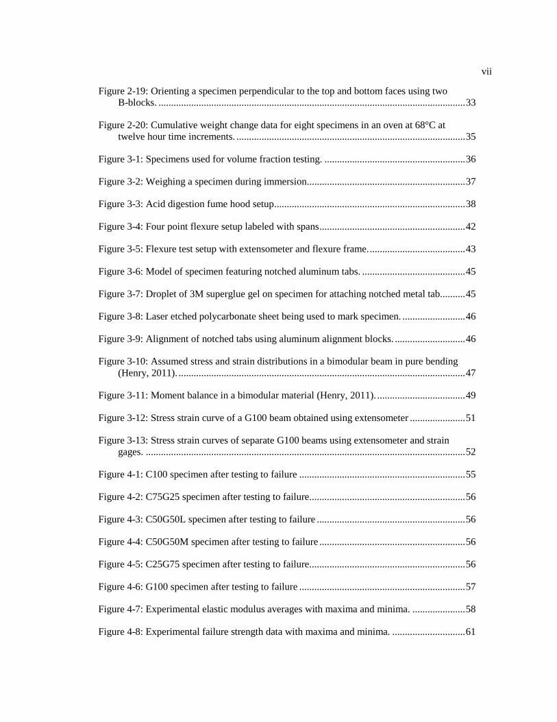
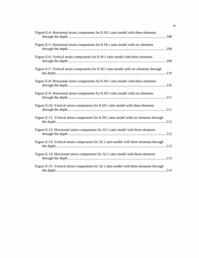
LIST OF FIGURES ................................................................................................................. vi

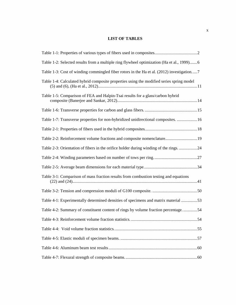
LIST OF TABLES ................................................................................................................... x

ACKNOWLEDGEMENTS ..................................................................................................... xiii

Chapter 1 Introduction ............................................................................................................ 1

1.1 Background ................................................................................................................ 1 1.2 Objectives and Scope ................................................................................................. 8 1.3 Literature Review ....................................................................................................... 8

Chapter 2 Specimen Fabrication ............................................................................................. 17

2.1 Materials..................................................................................................................... 17 2.2 Matrix Delivery .......................................................................................................... 21 2.3 Filament Winding ...................................................................................................... 23 2.4 Images of Rings and Beam Specimens ...................................................................... 27 2.5 Specimen Preparation................................................................................................. 29

Chapter 3 Test Methods .......................................................................................................... 36

3.1 Volume Fraction Testing............................................................................................ 36 3.2 Four Point Flexure Testing......................................................................................... 41

Chapter 4 Results .................................................................................................................... 53

4.1 Volume Fraction Data ................................................................................................ 53 4.2 Beam Test Results ...................................................................................................... 55 4.3 Transverse Moduli ..................................................................................................... 57 4.4 Transverse Strengths .................................................................................................. 60

Chapter 5 Analysis of Experimental Results .......................................................................... 62

5.1 Evaluation of Existing Models ................................................................................... 62 5.1.1 Series Spring Model ........................................................................................ 64 5.1.2 Modified Series Spring Model ........................................................................ 66 5.1.3 Modified Halpin-Tsai ...................................................................................... 68

5.2 Finite Element Analysis ............................................................................................. 69 5.3 Summary of Models ................................................................................................... 79

Chapter 6 Conclusions and Recommendations ....................................................................... 81

6.1 Conclusions ................................................................................................................ 81 6.2 Recommendations for Future Work ........................................................................... 82

v

References ................................................................................................................................ 85

Appendix A Electrical Setup of Mandrel Heater .................................................................... 90

Appendix B Acid Digestion Setup and Safety Measures........................................................ 96

Appendix C Volume Fraction Data for Individual Specimens ............................................... 98

Appendix D Flexural Test Results for Individual Specimens ................................................ 100

Appendix E Finite Element Study of Flexure Test Fixture..................................................... 103

Appendix F Nontechnical Abstract ......................................................................................... 115

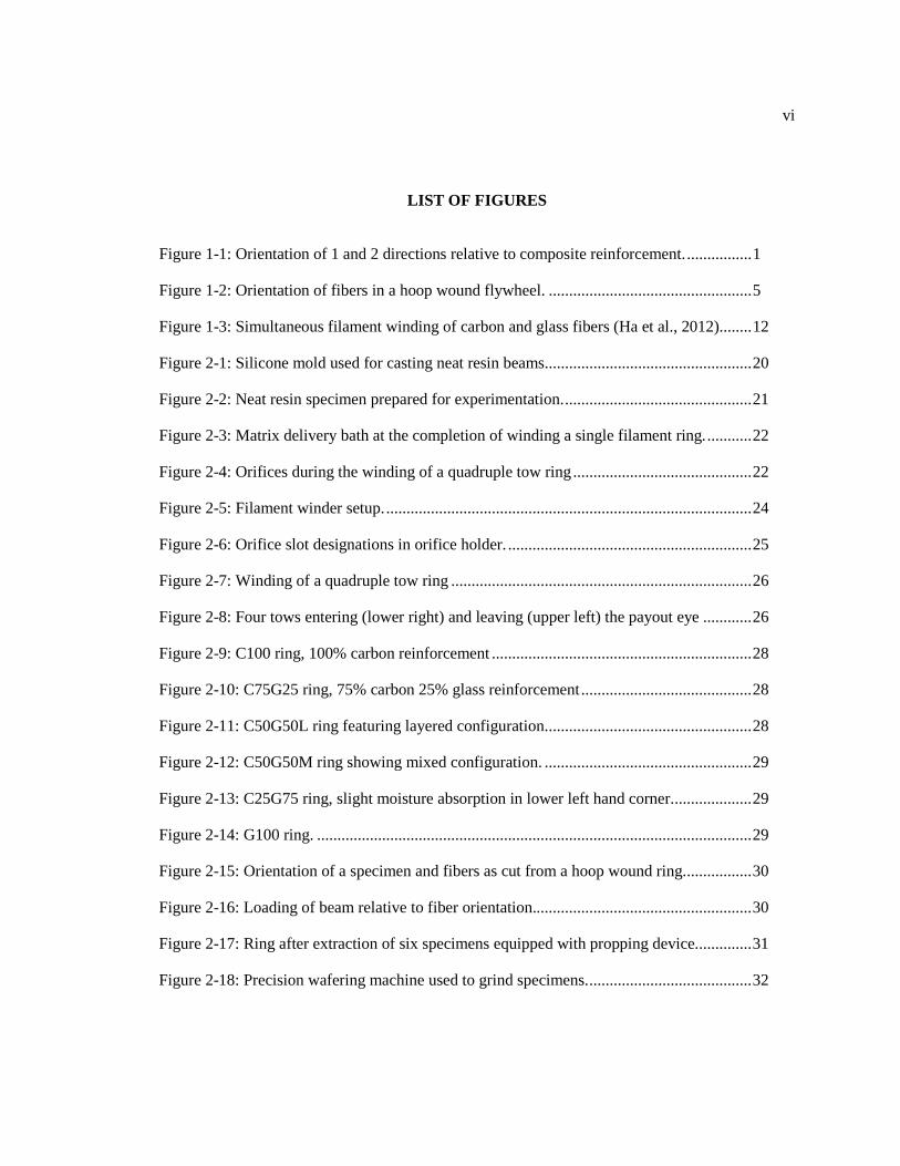
vi

LIST OF FIGURES

Figure 1-1: Orientation of 1 and 2 directions relative to composite reinforcement. ................ 1

Figure 1-2: Orientation of fibers in a hoop wound flywheel. .................................................. 5

Figure 1-3: Simultaneous filament winding of carbon and glass fibers (Ha et al., 2012). ....... 12

Figure 2-1: Silicone mold used for casting neat resin beams................................................... 20

Figure 2-2: Neat resin specimen prepared for experimentation. .............................................. 21

Figure 2-3: Matrix delivery bath at the completion of winding a single filament ring. ........... 22

Figure 2-4: Orifices during the winding of a quadruple tow ring ............................................ 22

Figure 2-5: Filament winder setup. .......................................................................................... 24

Figure 2-6: Orifice slot designations in orifice holder. ............................................................ 25

Figure 2-7: Winding of a quadruple tow ring .......................................................................... 26

Figure 2-8: Four tows entering (lower right) and leaving (upper left) the payout eye ............ 26

Figure 2-9: C100 ring, 100% carbon reinforcement ................................................................ 28

Figure 2-10: C75G25 ring, 75% carbon 25% glass reinforcement .......................................... 28

Figure 2-11: C50G50L ring featuring layered configuration. .................................................. 28

Figure 2-12: C50G50M ring showing mixed configuration. ................................................... 29

Figure 2-13: C25G75 ring, slight moisture absorption in lower left hand corner. ................... 29

Figure 2-14: G100 ring. ........................................................................................................... 29

Figure 2-15: Orientation of a specimen and fibers as cut from a hoop wound ring. ................ 30

Figure 2-16: Loading of beam relative to fiber orientation...................................................... 30

Figure 2-17: Ring after extraction of six specimens equipped with propping device. ............. 31

Figure 2-18: Precision wafering machine used to grind specimens. ........................................ 32

vii

Figure 2-19: Orienting a specimen perpendicular to the top and bottom faces using two B-blocks. .......................................................................................................................... 33

Figure 2-20: Cumulative weight change data for eight specimens in an oven at 68°C at twelve hour time increments. ........................................................................................... 35

Figure 3-1: Specimens used for volume fraction testing. ........................................................ 36

Figure 3-2: Weighing a specimen during immersion. .............................................................. 37

Figure 3-3: Acid digestion fume hood setup ............................................................................ 38

Figure 3-4: Four point flexure setup labeled with spans .......................................................... 42

Figure 3-5: Flexure test setup with extensometer and flexure frame. ...................................... 43

Figure 3-6: Model of specimen featuring notched aluminum tabs. ......................................... 45

Figure 3-7: Droplet of 3M superglue gel on specimen for attaching notched metal tab. ......... 45

Figure 3-8: Laser etched polycarbonate sheet being used to mark specimen. ......................... 46

Figure 3-9: Alignment of notched tabs using aluminum alignment blocks. ............................ 46

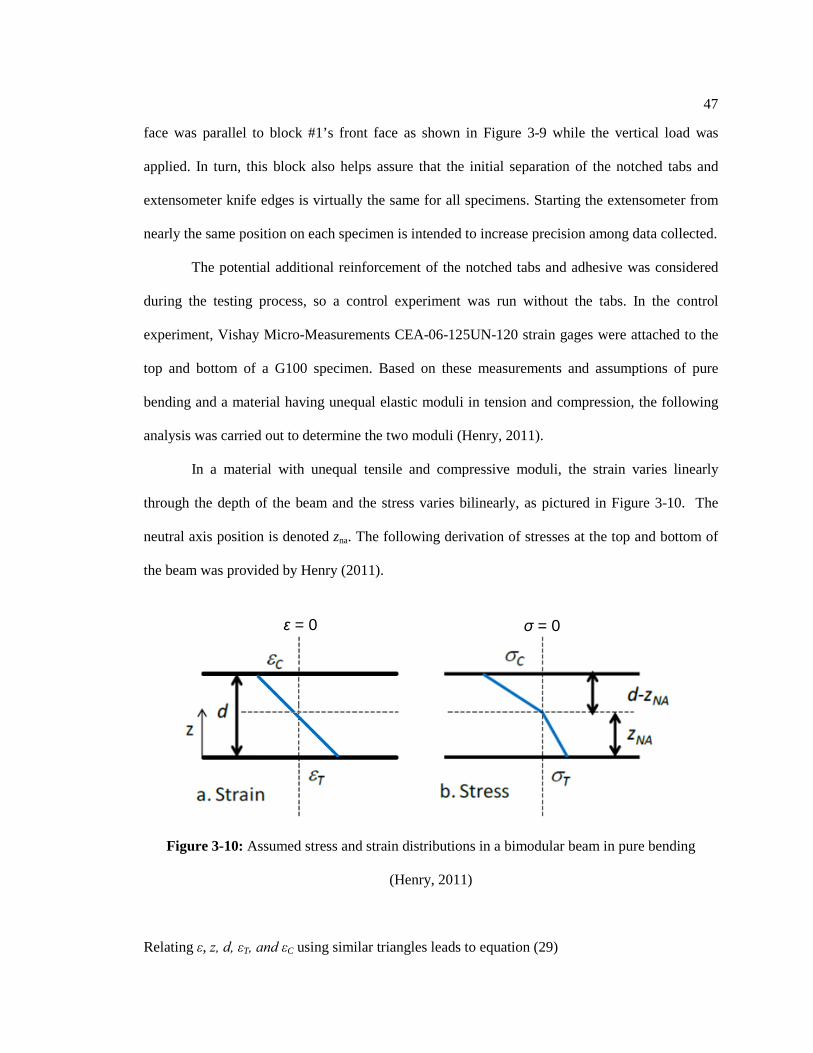
Figure 3-10: Assumed stress and strain distributions in a bimodular beam in pure bending (Henry, 2011). .................................................................................................................. 47

Figure 3-11: Moment balance in a bimodular material (Henry, 2011). ................................... 49

Figure 3-12: Stress strain curve of a G100 beam obtained using extensometer ...................... 51

Figure 3-13: Stress strain curves of separate G100 beams using extensometer and strain gages. ............................................................................................................................... 52

Figure 4-1: C100 specimen after testing to failure .................................................................. 55

Figure 4-2: C75G25 specimen after testing to failure. ............................................................. 56

Figure 4-3: C50G50L specimen after testing to failure ........................................................... 56

Figure 4-4: C50G50M specimen after testing to failure .......................................................... 56

Figure 4-5: C25G75 specimen after testing to failure. ............................................................. 56

Figure 4-6: G100 specimen after testing to failure .................................................................. 57

Figure 4-7: Experimental elastic modulus averages with maxima and minima. ..................... 58

Figure 4-8: Experimental failure strength data with maxima and minima. ............................. 61

viii

Figure 5-1: ROM for modulus of composite hybrids in the 1-direction. ................................. 63

Figure 5-2: Predictions of the series spring model compared to experimental data. ............... 65

Figure 5-3: MSSM results as compared to experimental data. ................................................ 67

Figure 5-4: MHTM results as compared to experimental data ................................................ 68

Figure 5-5: Boundary conditions with a free right edge, C100 model ..................................... 70

Figure 5-6: Boundary conditions with a constrained right edge, G100 model ........................ 71

Figure 5-7: Full view of the G100 model with 138417 elements ............................................ 73

Figure 5-8: A selected section of the G100 model with 138417 elements .............................. 73

Figure 5-9: Stress field showing stress components in the 2-direction (Y-direction) for the G100 model, rectangle over portion of model shown in Figure 5-10 .............................. 76

Figure 5-10: Symmetric portion of the G100 model used to compute stress partitioning parameters based on stress in the direction of loading (2- or Y-direction) ....................... 77

Figure 5-11: Graphical comparison of models used in the theoretical analysis....................... 80

Figure 6-1: Boundary conditions and parameters for suggested FE study .............................. 84

Figure A-1: Wiring schematic of ring heater circuit. ............................................................... 90

Figure A-2: One possible setup of the slip rings and brushes .................................................. 91

Figure A-3: Improper contact of brushes, the brush faces should be flush against the rings and no part of the face should be visible .......................................................................... 91

Figure A-4: Inserting the multimeter probes into the plug connected to the brushes. ............. 92

Figure A-5: Reading the resistance of the setup circuit ........................................................... 92

Figure A-6: Proper wiring of transformer ................................................................................ 94

Figure A-7: Transformer set to 60%, always set the transformer to 0% when touching the mandrel to avoid the hazardous potential. ........................................................................ 94

Figure B-1: Setup of acid digestion equipment. ...................................................................... 97

Figure E-1: Boundary conditions for the prescribed displacement FE model ......................... 104

Figure E-2: Boundary conditions for the prescribed load FE model ....................................... 104

Figure E-3: Locations of elements used to calculate strain...................................................... 105

ix

Figure E-4: Horizontal strain components for 8.18:1 ratio model with three elements through the depth ............................................................................................................. 108

Figure E-5: Horizontal strain components for 8.18:1 ratio model with six elements through the depth ............................................................................................................. 109

Figure E-6: Vertical strain components for 8.18:1 ratio model with three elements through the depth ............................................................................................................. 109

Figure E-7: Vertical strain components for 8.18:1 ratio model with six elements through the depth ........................................................................................................................... 110

Figure E-8: Horizontal stress components for 8.18:1 ratio model with three elements through the depth ............................................................................................................. 110

Figure E-9: Horizontal stress components for 8.18:1 ratio model with six elements through the depth ............................................................................................................. 111

Figure E-10: Vertical stress components for 8.18:1 ratio model with three elements through the depth ............................................................................................................. 111

Figure E-11: Vertical stress components for 8.18:1 ratio model with six elements through the depth ........................................................................................................................... 112

Figure E-12: Horizontal strain components for 32:1 ratio model with three elements through the depth ............................................................................................................. 112

Figure E-13: Vertical strain components for 32:1 ratio model with three elements through the depth ........................................................................................................................... 113

Figure E-14: Horizontal stress components for 32:1 ratio model with three elements through the depth ............................................................................................................. 113

Figure E-15: Vertical stress components for 32:1 ratio model with three elements through the depth ........................................................................................................................... 114

x

LIST OF TABLES

Table 1-1: Properties of various types of fibers used in composites. ....................................... 2

Table 1-2: Selected results from a multiple ring flywheel optimization (Ha et al., 1999). ...... 6

Table 1-3: Cost of winding commingled fiber rotors in the Ha et al. (2012) investigation. .... 7

Table 1-4: Calculated hybrid composite properties using the modified series spring model (5) and (6), (Ha et al., 2012)............................................................................................. 11

Table 1-5: Comparison of FEA and Halpin-Tsai results for a glass/carbon hybrid composite (Banerjee and Sankar, 2012). .......................................................................... 14

Table 1-6: Transverse properties for carbon and glass fibers. ................................................. 15

Table 1-7: Transverse properties for non-hybridized unidirectional composites. ................... 16

Table 2-1: Properties of fibers used in the hybrid composites. ................................................ 18

Table 2-2: Reinforcement volume fractions and composite nomenclature.............................. 19

Table 2-3: Orientation of fibers in the orifice holder during winding of the rings. ................. 24

Table 2-4: Winding parameters based on number of tows per ring. ........................................ 27

Table 2-5: Average beam dimensions for each material type. ................................................. 34

Table 3-1: Comparison of mass fraction results from combustion testing and equations (22) and (24)..................................................................................................................... 41

Table 3-2: Tension and compression moduli of G100 composite. .......................................... 50

Table 4-1: Experimentally determined densities of specimens and matrix material ............... 53

Table 4-2: Summary of constituent content of rings by volume fraction percentage. ............. 54

Table 4-3: Reinforcement volume fraction statistics. .............................................................. 54

Table 4-4: Void volume fraction statistics. ............................................................................. 55

Table 4-5: Elastic moduli of specimen beams. ........................................................................ 57

Table 4-6: Aluminum beam test results ................................................................................... 60

Table 4-7: Flexural strength of composite beams. ................................................................... 60

xi

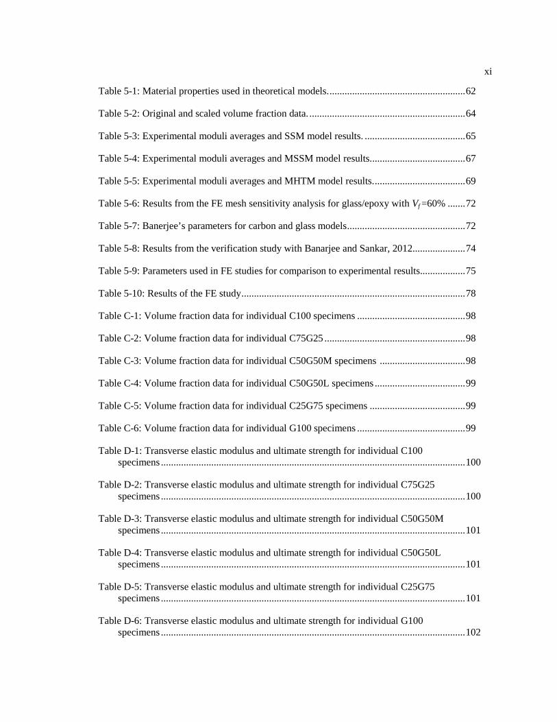
Table 5-1: Material properties used in theoretical models. ...................................................... 62

Table 5-2: Original and scaled volume fraction data. .............................................................. 64

Table 5-3: Experimental moduli averages and SSM model results. ........................................ 65

Table 5-4: Experimental moduli averages and MSSM model results. ..................................... 67

Table 5-5: Experimental moduli averages and MHTM model results. .................................... 69

Table 5-6: Results from the FE mesh sensitivity analysis for glass/epoxy with Vf =60% ....... 72

Table 5-7: Banerjee’s parameters for carbon and glass models ............................................... 72

Table 5-8: Results from the verification study with Banarjee and Sankar, 2012. .................... 74

Table 5-9: Parameters used in FE studies for comparison to experimental results. ................. 75

Table 5-10: Results of the FE study ......................................................................................... 78

Table C-1: Volume fraction data for individual C100 specimens ........................................... 98

Table C-2: Volume fraction data for individual C75G25 ........................................................ 98

Table C-3: Volume fraction data for individual C50G50M specimens .................................. 98

Table C-4: Volume fraction data for individual C50G50L specimens .................................... 99

Table C-5: Volume fraction data for individual C25G75 specimens ...................................... 99

Table C-6: Volume fraction data for individual G100 specimens ........................................... 99

Table D-1: Transverse elastic modulus and ultimate strength for individual C100 specimens ......................................................................................................................... 100

Table D-2: Transverse elastic modulus and ultimate strength for individual C75G25 specimens ......................................................................................................................... 100

Table D-3: Transverse elastic modulus and ultimate strength for individual C50G50M specimens ......................................................................................................................... 101

Table D-4: Transverse elastic modulus and ultimate strength for individual C50G50L specimens ......................................................................................................................... 101

Table D-5: Transverse elastic modulus and ultimate strength for individual C25G75 specimens ......................................................................................................................... 101

Table D-6: Transverse elastic modulus and ultimate strength for individual G100 specimens ......................................................................................................................... 102

xii

Table D-7: Elastic modulus for individual neat resin specimens ............................................. 102

Table E-1: Experimental parameters from G100-2 test used in FE study ............................... 103

Table E-2: Data from the prescribed load FE study ................................................................. 106

Table E-3: Data from the prescribed displacement FE study .................................................. 107

Table E-4: Parameters from the FE support span to depth ratio study .................................... 107

xiii

ACKNOWLEDGEMENTS

I would like to thank Dr. Charles E. Bakis for his time spent carefully advising me

throughout this investigation. His exceptional ability to incredibly frequently meet with me on

extremely short notice to discuss questions or the many theories that I had during the research

process was critical toward promoting continual progress. Finally, his persistent encouragement

and previous experience with composites made the accurate completion of this investigation

possible.

The sponsor of this project was the U.S. DOE/NETL and the award number was DE-

EE000575. My fellowship was awarded through the Penn State GATE Center of Excellence: In-

Vehicle, High-Power Energy Storage Technologies. I would like to extend my gratitude toward

the GATE program and Dr. Joel Anstrom for making it possible to find this fellowship.

I would like to thank Mr. Todd C. Henry for diligently training me to operate the winding

equipment, testing equipment, and data acquisition setups. I would also like to recognize his

continual generosity for voluntarily offering insight toward the analytical portion of my project

and providing moral support when times were tough.

I extend my personal thanks to Dr. Thomas Juska for his advice on material decisions and

generous loans of equipment for extended periods of time.

1

Chapter 1

Introduction

1.1 Background

Composites offer many benefits over common engineering materials because of their

high strength to weight ratio. However, they present design challenges since they are highly

anisotropic. This anisotropy requires material properties to be defined in multiple directions

relative to the constituents of the composite. When the elastic moduli of a composite are tested in

the longitudinal and transverse directions, the results often differ by two orders of magnitude.

This large difference in directional properties creates the need to carefully design a composite

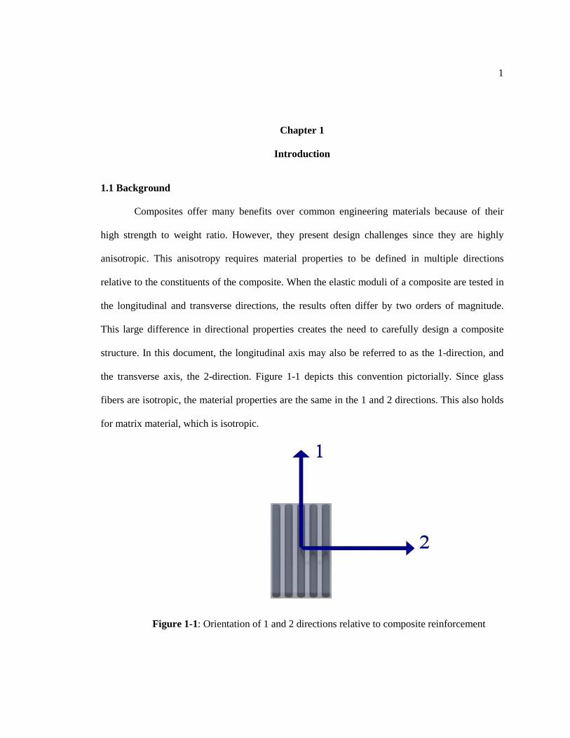
structure. In this document, the longitudinal axis may also be referred to as the 1-direction, and

the transverse axis, the 2-direction. Figure 1-1 depicts this convention pictorially. Since glass

fibers are isotropic, the material properties are the same in the 1 and 2 directions. This also holds

for matrix material, which is isotropic.

Figure 1-1: Orientation of 1 and 2 directions relative to composite reinforcement

2

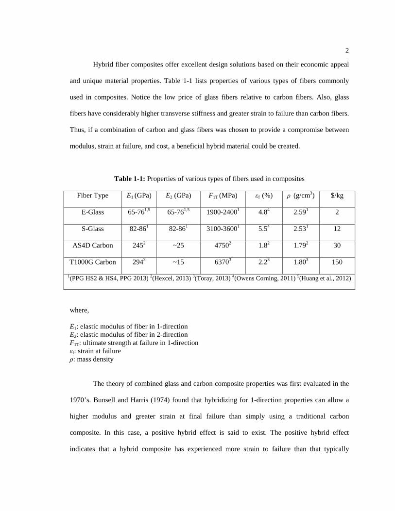
Hybrid fiber composites offer excellent design solutions based on their economic appeal

and unique material properties. Table 1-1 lists properties of various types of fibers commonly

used in composites. Notice the low price of glass fibers relative to carbon fibers. Also, glass

fibers have considerably higher transverse stiffness and greater strain to failure than carbon fibers.

Thus, if a combination of carbon and glass fibers was chosen to provide a compromise between

modulus, strain at failure, and cost, a beneficial hybrid material could be created.

Table 1-1: Properties of various types of fibers used in composites

Fiber Type E1 (GPa) E2 (GPa) F1T (MPa) εf (%) ρ (g/cm3) $/kg

E-Glass 65-761,5 65-761,5 1900-24001 4.84 2.591 2

S-Glass 82-861 82-861 3100-36001 5.54 2.531 12

AS4D Carbon 2452 ~25 47502 1.82 1.792 30

T1000G Carbon 2943 ~15 63703 2.23 1.803 150

1(PPG HS2 & HS4, PPG 2013) 2(Hexcel, 2013) 3(Toray, 2013) 4(Owens Corning, 2011) 5(Huang et al., 2012)

where,

E1: elastic modulus of fiber in 1-direction E2: elastic modulus of fiber in 2-direction F1T: ultimate strength at failure in 1-direction εf: strain at failure ρ: mass density

The theory of combined glass and carbon composite properties was first evaluated in the

1970’s. Bunsell and Harris (1974) found that hybridizing for 1-direction properties can allow a

higher modulus and greater strain at final failure than simply using a traditional carbon

composite. In this case, a positive hybrid effect is said to exist. The positive hybrid effect

indicates that a hybrid composite has experienced more strain to failure than that typically

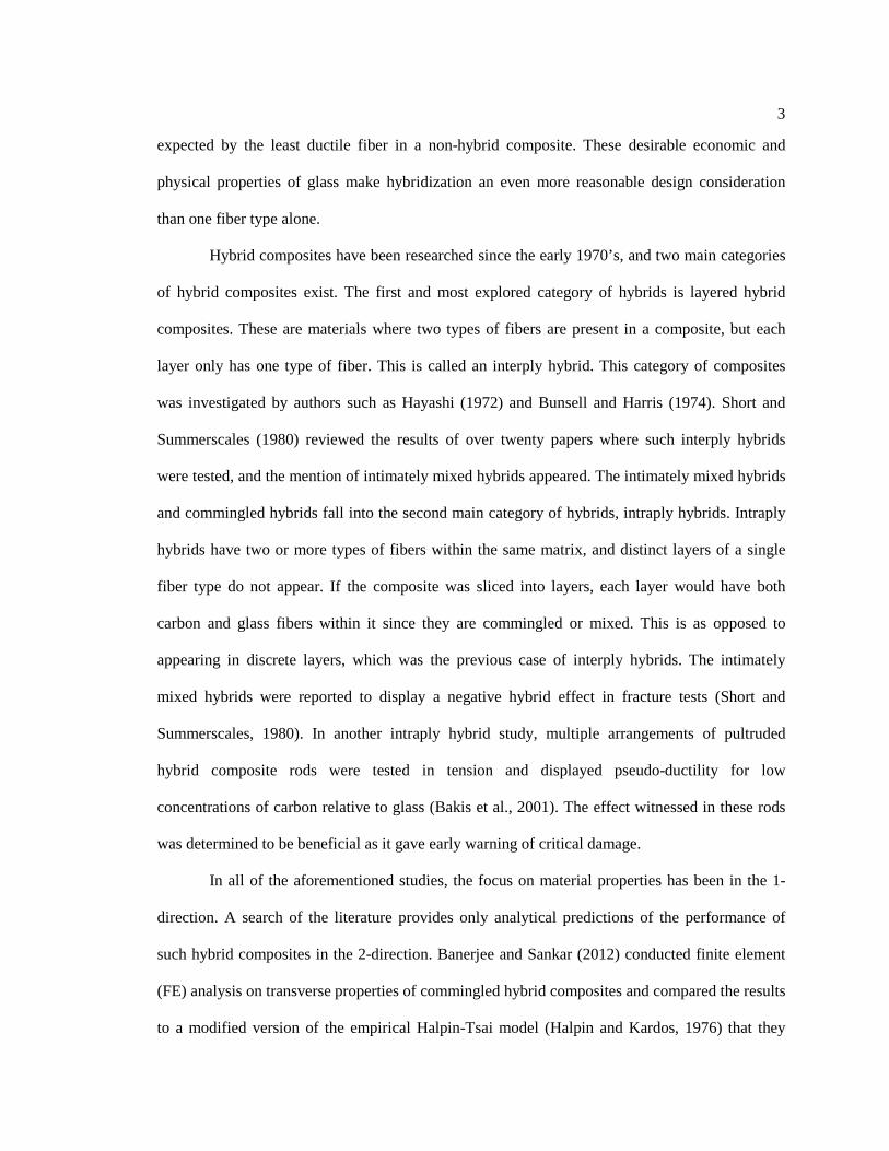
3

expected by the least ductile fiber in a non-hybrid composite. These desirable economic and

physical properties of glass make hybridization an even more reasonable design consideration

than one fiber type alone.

Hybrid composites have been researched since the early 1970’s, and two main categories

of hybrid composites exist. The first and most explored category of hybrids is layered hybrid

composites. These are materials where two types of fibers are present in a composite, but each

layer only has one type of fiber. This is called an interply hybrid. This category of composites

was investigated by authors such as Hayashi (1972) and Bunsell and Harris (1974). Short and

Summerscales (1980) reviewed the results of over twenty papers where such interply hybrids

were tested, and the mention of intimately mixed hybrids appeared. The intimately mixed hybrids

and commingled hybrids fall into the second main category of hybrids, intraply hybrids. Intraply

hybrids have two or more types of fibers within the same matrix, and distinct layers of a single

fiber type do not appear. If the composite was sliced into layers, each layer would have both

carbon and glass fibers within it since they are commingled or mixed. This is as opposed to

appearing in discrete layers, which was the previous case of interply hybrids. The intimately

mixed hybrids were reported to display a negative hybrid effect in fracture tests (Short and

Summerscales, 1980). In another intraply hybrid study, multiple arrangements of pultruded

hybrid composite rods were tested in tension and displayed pseudo-ductility for low

concentrations of carbon relative to glass (Bakis et al., 2001). The effect witnessed in these rods

was determined to be beneficial as it gave early warning of critical damage.

In all of the aforementioned studies, the focus on material properties has been in the 1-

direction. A search of the literature provides only analytical predictions of the performance of

such hybrid composites in the 2-direction. Banerjee and Sankar (2012) conducted finite element

(FE) analysis on transverse properties of commingled hybrid composites and compared the results

to a modified version of the empirical Halpin-Tsai model (Halpin and Kardos, 1976) that they

4

developed. Banerjee and Sankar’s modified Halpin-Tsai model adds an additional set of terms for

a second fiber type. Ha et al. (2012) presented an micromechanical model for the transverse

modulus of unidirectional hybrid composites with parameters based on experimental results not

included in the publication. Ko and Ju (2013) developed a series of higher-order micromechanical

models for transverse elastic properties of unidirectional hybrid composites that consider various

complicating factors such as fiber interaction, fiber size, and fiber distribution. No experimental

data on unidirectional hybrid fiber composites could be found in the literature.

One important use for glass and carbon fiber composites is high speed flywheel design.

High speed flywheels may be used for kinetic energy storage. For this application, the maximum

energy density is possibly the most important design criteria. To achieve a high energy density

flywheel, the material properties and rotor geometry must be carefully selected. Genta (1985)

provides a simple equation (1) based on this concept for an isotropic rotor’s kinetic energy.

𝐸𝑚

= 𝐾𝜎𝜌

(1)

where,

E: kinetic energy of the rotor m: the rotor’s mass K: the rotor’s geometric shape factor σ: the tensile strength of the material ρ: the material’s density

According to equation (1), the ideal materials for flywheels are high of strength and low density.

Because flywheels have the highest stress in the hoop direction, the fibers in composite flywheel

are therefore generally oriented in the hoop direction, as pictured in Figure 1-2, which provides

the maximum energy storage capability per unit mass.

5

Figure 1-2: Orientation of fibers in a hoop wound flywheel

Figure 1-2 shows the most popular fiber configuration for composite flywheels designed

for energy storage. However, research has shown that an optimal design may be reached by

assembling multiple rings of different materials and creating a hybrid flywheel. Table 1-2 shows

the computational results from an optimization study of multiple ring hybrid flywheels with

increasing hoop direction modulus and tensile strength in rings located at increasing radii.

6

Table 1-2: Selected results from a multiple ring flywheel optimization by Ha et al. (1999)

Case Material Sequence Total Stored Energy (Wh)

1-3 E 1125

2-1 A-E 1837

3-1 A-C-E 1973

4-1 A-B-C-E 2013

Materials: A – Glass/Epoxy B – Kevlar/Epoxy

C – AS/H3501 D – T300/5208 E – IM6/Epoxy

In Table 1-2, it is seen that the total stored energy (TSE), is highest for Case 4-1, a four

ring flywheel. Although Case 3-1, a three ring flywheel, is a close second highest TSE, the most

impressive energy storage less than Case 4-1 is Case 2-1. In Case 2-1, which had only two rings,

1837 Wh of energy was stored. This is a major improvement over any of the results from Case 1,

and is not far behind the best of Cases 3 and 4.

After seeing results such as these, the next logical topic of research would be to design

flywheels composed of commingled fibers, as opposed to flywheels composed of distinct rings of

different fibers. Ha et al. (2012) optimized and fabricated a commingled fiber composite hybrid

rotor which was a compromise of performance and cost. Their reinforcement fiber volume

percentages from inner rim to outer for four rings were as follows (carbon/glass): 11%/89%,

30%/70%, 79%/21%, 100%/0%. The aim of this design is to gradually increase hoop direction

modulus and tensile strength with increasing radius. One weakness of this optimization was the

use of calculated transverse properties for the hybrid materials. The only experimental data

mentioned was for the transverse tensile strength of the hybrid rims considering only the matrix

7

effect. The economic benefit of winding these rotors with commingled fibers was lightly explored

for the three cases in Table 1-3.

Table 1-3: Cost of winding commingled fiber rotors in the Ha et al. (2012) investigation

Case Cost Process

Case A $25,000 All rims wound simultaneously

Case B $44,000 Interference fitting of each separately wound rim

Case C $31,000 Two rims of commingled fibers are wound separately

and press fit together

The three case studies included in Table1-3 show that it is most economical to wind all of

the rims simultaneously, such as in Case A. However, in Case A, Ha et al. (2012) found that

thermal residual stresses from winding all of the rims simultaneously have a devastating effect on

rotor performance. Case B is the most expensive procedure since all of the rims are wound

separately and must be press fit together. Case C was chosen to be manufactured as it was the

intermediate between Cases A and B in terms of strength ratio and cost.

The literature discussed above has focused on the longitudinal elastic and strength

properties of hybrid fiber composites. In filament wound hybrid fiber composites for flywheel

energy systems, however, the transverse (radial) properties of commingled hybrid fiber

composites are of high importance as well. No experimental data on these properties were able to

be found in the literature.

8

1.2 Objectives and Scope

The objective of the current investigation is to experimentally determine the transverse

mechanical properties of hybrid filament wound glass and carbon fiber reinforced epoxy

composites as a function of reinforcement content. Five configurations of composites were tested

in four point flexure with the following approximate fiber contents by volume: 100% carbon,

75% carbon/25% glass, 50% carbon/50% glass, 25% carbon/75% glass, and 100% glass. The

100% rings were created to give upper and lower bounds on the properties, and were compared to

well established, non-hybridized composite properties. Neat resin specimens were also tested so

that the matrix material could be modeled in the finite element (FE) analysis. The composite

specimen properties to be determined are: transverse elastic modulus (E2), transverse failure

strength (F2T), fiber volume content (Vr), matrix volume content (Vm), void volume content (Vv),

and specimen density (ρc). Matrix density (ρm) was also to be determined from the fabrication of

neat resin specimens. The fiber volume content was determined using acid digestion and carbon

fiber combustion. The measured moduli were compared to the predicted moduli using the

following models: rule of mixtures, modified series spring model, and modified Halpin Tsai. A

FE analysis was conducted on a hexagonal array of approximately 100 fibers for the 100% carbon

and 100% glass reinforcement composites. The FE results were compared to the experimental

results and model predictions.

1.3 Literature Review

Publications in the area of hybrid fiber reinforced composites have focused on

determining properties in the 1-direction. One of the most basic equations for estimating material

properties, the rule of mixtures, has been shown to work well for composite hybrids in the 1-

9

direction. Originally, the rule of mixtures was developed to predict the modulus in the 1-direction

of single fiber composites. Daniel and Ishai (2006), wrote, “Assuming a perfect bond between

matrix and fibers, longitudinal strains are uniform throughout and equal for the matrix and fibers.

This leads to the so called rule of mixtures or parallel model for the longitudinal modulus.” For

this reason, the rule of mixtures is also known as the iso-strain model. This model gives ideal

results, and is a theoretical upper bound for the expected properties. The rule of mixtures is

defined for elastic modulus is as follows (2):

where,

𝐸𝑠 = 𝐸𝑓𝑉𝑓 + 𝐸𝑚𝑉𝑚 (2)

Es: elastic modulus of composite system Ef/m: elastic modulus of fiber or matrix Vf/m: volume fraction of fiber or matrix The rule of mixtures is considered appropriate for estimates of the 1-direction elastic

moduli of layered hybrid composites (Marom et al., 1978; Bunsell and Harris, 1974). The

commingled fiber modified version of the rule of mixtures is given by equation (3).

𝐸𝑐 = 𝐸𝑓1𝑉𝑓1 + 𝐸𝑓2𝑉𝑓2 + 𝐸𝑚𝑉𝑚 (3)

where,

f1/2: respective property for fiber 1 or 2

Although these equations do not have terms for void content, actual composites

inevitably have void content. The presence of voids causes a decrease in material properties such

as elastic modulus and failure strength.

The series spring model is a more accurate model to use for the prediction of composite

transverse modulus properties, because it operates under the assumption of isostress. The isostress

10

assumption is a more accurate representation of the loading provided to a composite’s

constituents in the transverse direction than the isostrain assumption. The series spring model for

a composite with only one type of fiber is given by equation (4).

1𝐸𝑐

=𝑉𝑓𝐸𝑓

+𝑉𝑚𝐸𝑚

(4)

The series spring model adopted for hybrid composites (5) is considered a lower bound for the

prediction of composite modulus.

1𝐸𝑐

= 𝑉𝑟,𝑐

𝐸𝑐+𝑉𝑟,𝑔

𝐸𝑔+𝑉𝑚𝐸𝑚

(5)

where,

Ec: modulus of the composite Vr,c: volume fraction of carbon reinforcement in sample (%) Vr,g: volume fraction of glass reinforcement in sample (%) Vm: volume fraction of matrix in sample (%) Eg: modulus of glass fiber Ec: modulus of carbon fiber Em: modulus of matrix

Ha et al. (2012) used the modified version of the series spring model (6) and (7) to estimate the

transverse modulus of commingled hybrid composites in the 2-direction.

1𝐸2

= 𝑉𝑚𝐸2𝑚

+𝜂𝑔𝑉𝑔𝐸2𝑔

+𝜂𝑐𝑉𝑐𝐸2𝑐

/ 𝑉𝑚 + 𝜂𝑔𝑉𝑔 + 𝜂𝑐𝑉𝑐 (6)

𝜂𝑔 =𝜎𝑔𝜎𝑚

𝑎𝑛𝑑 𝜂𝑐 =𝜎𝑐𝜎𝑚

(7)

where,

11

σg: average stress distribution in glass fiber σc: average stress distribution in carbon fiber σm: average stress distribution in matrix ηg: glass composite stress partitioning parameter ηc: carbon composite stress partitioning parameter Vc: volume fraction of carbon Vg: volume fraction of glass

In this model, the stress partitioning parameter η, is defined as the ratio of stress in the fiber

divided by stress in the matrix. The calculated results for the transverse modulus of the modified

series spring model for a few hybrids are shown in Table 1-4. The transverse moduli assumed for

glass and carbon fibers were 72 GPa and 23 GPa, respectively. The elastic moduli in the 2-

direction monotonically decrease with an increasing proportion of carbon fiber, as expected. Ha

et al. (2012) experimentally determined η to be 3.78 and 1.48 for glass and carbon composites,

respectively, although evidence supporting the validity of these values for hybrid fiber

composites was not presented.

Table 1-4: Calculated hybrid composite properties using the

modified series spring model (6) and (7) (Ha et al., 2012)

Carbon Reinforcement (%) Glass Reinforcement (%) Calculated E2 (GPa)

10 90 19.5 11 89 19.4 30 70 17.0 35 65 16.5 40 60 16.0 66 34 13.0 72 28 12.0 79 21 11.0

Using the results of Table 1-4, Ha et al. (2012) successfully designed and manufactured

hybrid filament wound flywheel rims for a larger composite rotor assembly. The larger rotor

12

assembly would normally have been made from twice as many rims, increasing the product’s

complexity. By producing rims that were initially hybridized, they reduced the total number of

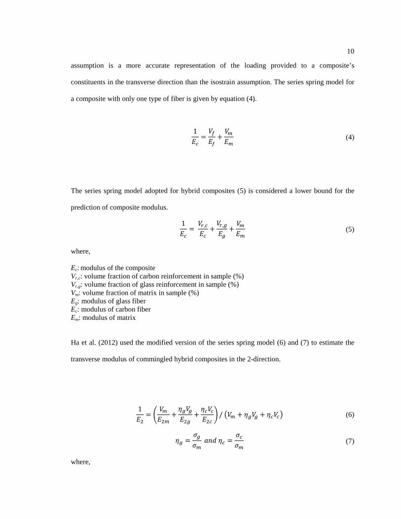
rims in the rotor, and obtained a compromise of material properties. Figure 1-3 shows a

photograph of their hybrid winding process. In the photograph a wide band of fibers is shown,

and the fibers alternate between carbon and glass. The fibers are lying in a solid band that appears

to have negligible gaps between fibers. This is desired during winding because it provides a high

quality part with low void volume and higher properties than a part produced with gaps between

the fibers.

Figure 1-3: Simultaneous filament winding of carbon and glass fibers (Ha et al., 2012)

Banerjee and Sankar (2012) performed a finite element analysis of transverse mechanical

properties of commingled fiber hybrid composites. The results agreed well with their version of

the modified Halpin-Tsai equations. The single fiber Halpin-Tsai equations are given by (8) and

(9).

𝐸2𝐸𝑚

=1 + 𝜉𝜂𝑉𝑓1 − 𝜂𝑉𝑓

(8)

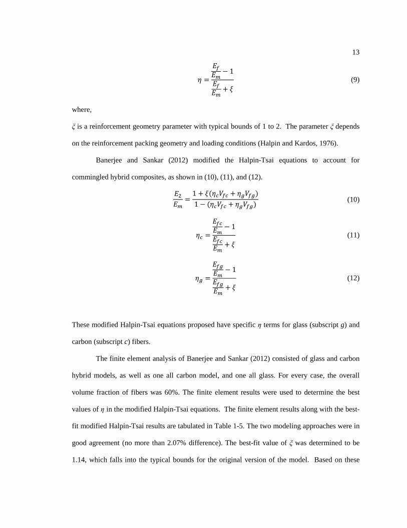
13

𝜂 =

𝐸𝑓𝐸𝑚

− 1

𝐸𝑓𝐸𝑚

+ 𝜉 (9)

where,

ξ is a reinforcement geometry parameter with typical bounds of 1 to 2. The parameter ξ depends

on the reinforcement packing geometry and loading conditions (Halpin and Kardos, 1976).

Banerjee and Sankar (2012) modified the Halpin-Tsai equations to account for

commingled hybrid composites, as shown in (10), (11), and (12).

𝐸2𝐸𝑚

=1 + 𝜉(𝜂𝑐𝑉𝑓𝑐 + 𝜂𝑔𝑉𝑓𝑔)1 − (𝜂𝑐𝑉𝑓𝑐 + 𝜂𝑔𝑉𝑓𝑔)

(10)

𝜂𝑐 =

𝐸𝑓𝑐𝐸𝑚

− 1

𝐸𝑓𝑐𝐸𝑚

+ 𝜉 (11)

𝜂𝑔 =

𝐸𝑓𝑔𝐸𝑚

− 1

𝐸𝑓𝑔𝐸𝑚

+ 𝜉 (12)

These modified Halpin-Tsai equations proposed have specific η terms for glass (subscript g) and

carbon (subscript c) fibers.

The finite element analysis of Banerjee and Sankar (2012) consisted of glass and carbon

hybrid models, as well as one all carbon model, and one all glass. For every case, the overall

volume fraction of fibers was 60%. The finite element results were used to determine the best

values of η in the modified Halpin-Tsai equations. The finite element results along with the best-

fit modified Halpin-Tsai results are tabulated in Table 1-5. The two modeling approaches were in

good agreement (no more than 2.07% difference). The best-fit value of ξ was determined to be

1.14, which falls into the typical bounds for the original version of the model. Based on these

14

results, Banerjee and Sankar concluded that the modified version of the Halpin-Tsai equations

could be used to predict hybrid composite transverse moduli.

Table 1-5: Comparison of FEA and Halpin-Tsai results for a glass/carbon hybrid composite

(Banerjee and Sankar, 2012)

E2

Composite Vr,c (%) Vr,g (%) FEA (GPa) Halpin-Tsai (GPa) Difference (%) Carbon/Epoxy 60 0 8.77 8.59 2.07

Carbon and Glass Epoxy

Hybrids

54 6 9.05 8.88 1.84 42 18 9.66 9.52 1.47 30 30 10.33 10.22 1.08 18 42 11.05 11 0.5 6 54 11.82 11.86 -0.37

Glass/Epoxy 0 60 12.21 12.33 -1.02

Experimental transverse properties of hybrid composites have not been reported to-date,

as a search of the literature shows. Nevertheless, transverse properties for carbon and glass fibers

have been found, such as in Table 1-6. Table 1-6 displays the extreme difference between carbon

and glass fiber moduli in the transverse direction.

15

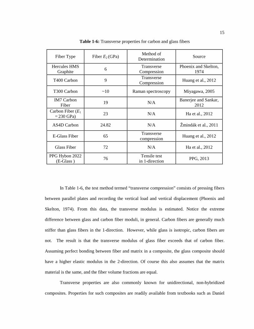
Table 1-6: Transverse properties for carbon and glass fibers

Fiber Type Fiber E2 (GPa) Method of Determination Source

Hercules HMS Graphite 6 Transverse

Compression Phoenix and Skelton,

1974

T400 Carbon 9 Transverse Compression Huang et al., 2012

T300 Carbon ~10 Raman spectroscopy Miyagawa, 2005

IM7 Carbon Fiber 19 N/A Banerjee and Sankar,

2012 Carbon Fiber (E1

= 230 GPa) 23 N/A Ha et al., 2012

AS4D Carbon 24.82 N/A Žmindák et al., 2011

E-Glass Fiber 65 Transverse compression Huang et al., 2012

Glass Fiber 72 N/A Ha et al., 2012

PPG Hybon 2022 (E-Glass ) 76 Tensile test

in 1-direction PPG, 2013

In Table 1-6, the test method termed “transverse compression” consists of pressing fibers

between parallel plates and recording the vertical load and vertical displacement (Phoenix and

Skelton, 1974). From this data, the transverse modulus is estimated. Notice the extreme

difference between glass and carbon fiber moduli, in general. Carbon fibers are generally much

stiffer than glass fibers in the 1-direction. However, while glass is isotropic, carbon fibers are

not. The result is that the transverse modulus of glass fiber exceeds that of carbon fiber.

Assuming perfect bonding between fiber and matrix in a composite, the glass composite should

have a higher elastic modulus in the 2-direction. Of course this also assumes that the matrix

material is the same, and the fiber volume fractions are equal.

Transverse properties are also commonly known for unidirectional, non-hybridized

composites. Properties for such composites are readily available from textbooks such as Daniel

16

and Ishai (2006). Table 1-7 has transverse modulus and tensile strength properties for carbon and

glass-based composites.

Table 1-7: Transverse properties for non-hybridized unidirectional composites

Composite Test Method E2(GPa) F2T(MPa) Vr (%)

E-Glass/Epoxy1 Tension 10.4 39 55 S-Glass/Epoxy1 Tension 11.0 49 50

Carbon/Epoxy (AS4/3501-6)1 Tension 10.3 57 63 Carbon/Epoxy (IM7/977-3)1 Tension 9.9 62 65

Carbon/Epoxy (IM6G/3501-6)1 Tension 9.0 46 66 E-Glass/DER 3833 Flexure 15.3 67.2 66

T800/RF0164 Flexure 8.53 48.4 64.3 T700/RF0074 Flexure 8.2 35.5 66 T700/RF0334 Flexure 8.52 31.5 66* T700/RF0314 Flexure 9.4 48.3 67

KS161-154/Epoxy5 Flexure 17.0 92.9 69.2 KS161-154/Epoxy5 Tension 18.3 40.7 69.2 AS4D/EPON 8622 Flexure 9.09 46.7 70 AS4C/EPON 94053 Flexure 8.9 77.3 70

AS4C/DER 3833 Flexure 10.0 71.7 70 1Daniel and Ishai (2006) 2 Henry (2011)

3Gabrys (1996)

4Sharma (2006) 5Deng et al. (1999) *estimated value

17

Chapter 2

Specimen Fabrication

2.1 Materials

The glass fiber chosen for this investigation is PPG Hybon 2022, Product Code 13053-

34098, E-Glass Roving of 1100 tex. This fiber is a single end E-Glass roving containing boron

with a silane sizing of 0.55 percent by weight. PPG specifies that it is for filament winding and

weaving or knitting. It is specifically compatible with epoxy resin systems. This fiber is designed

for applications requiring maximum wet out and wet out consistency (PPG, 2013). Based on

private correspondence with Bruce Parson of PPG Industries, the density of Hybon 2022 was

reported to be within 2.54-2.60 g/cc. The density used for glass fiber was taken to be 2.6172 g/cc,

from a helium pycnometry measurement of a study aimed at accurately determining the actual

density of E-glass fibers (Strait and Rude, 1998).

Hexcel HexTow AS4D-GP-12K carbon fiber tow was selected to be the carbon fiber for

this investigation. This product is a continuous, high strength, high strain, PAN based fiber with

12,000 filaments in a tow (Hexcel, 2013). Filament winding is one of Hexcel’s suggested uses of

this tow. The transverse modulus of this fiber is not reported by Hexcel. The extended properties

of fibers mentioned above are summarized in Table 2-1.

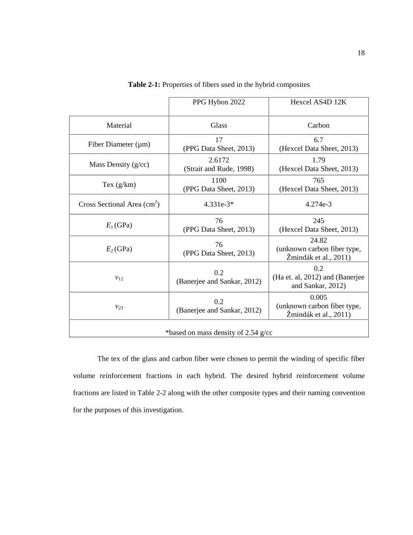
18

Table 2-1: Properties of fibers used in the hybrid composites

PPG Hybon 2022 Hexcel AS4D 12K

Material Glass Carbon

Fiber Diameter (µm) 17 (PPG Data Sheet, 2013)

6.7 (Hexcel Data Sheet, 2013)

Mass Density (g/cc) 2.6172 (Strait and Rude, 1998)

1.79 (Hexcel Data Sheet, 2013)

Tex (g/km) 1100 (PPG Data Sheet, 2013)

765 (Hexcel Data Sheet, 2013)

Cross Sectional Area (cm2) 4.331e-3* 4.274e-3

E1 (GPa) 76 (PPG Data Sheet, 2013)

245 (Hexcel Data Sheet, 2013)

E2 (GPa) 76 (PPG Data Sheet, 2013)

24.82 (unknown carbon fiber type,

Žmindák et al., 2011)

v12 0.2

(Banerjee and Sankar, 2012)

0.2 (Ha et. al, 2012) and (Banerjee

and Sankar, 2012)

v23 0.2

(Banerjee and Sankar, 2012)

0.005 (unknown carbon fiber type,

Žmindák et al., 2011)

*based on mass density of 2.54 g/cc

The tex of the glass and carbon fiber were chosen to permit the winding of specific fiber

volume reinforcement fractions in each hybrid. The desired hybrid reinforcement volume

fractions are listed in Table 2-2 along with the other composite types and their naming convention

for the purposes of this investigation.

19

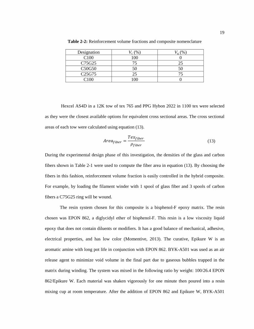
Table 2-2: Reinforcement volume fractions and composite nomenclature

Designation Vc (%) Vg (%) C100 100 0

C75G25 75 25 C50G50 50 50 C25G75 25 75

C100 100 0

Hexcel AS4D in a 12K tow of tex 765 and PPG Hybon 2022 in 1100 tex were selected

as they were the closest available options for equivalent cross sectional areas. The cross sectional

areas of each tow were calculated using equation (13).

𝐴𝑟𝑒𝑎𝑓𝑖𝑏𝑒𝑟 =𝑇𝑒𝑥𝑓𝑖𝑏𝑒𝑟

𝜌𝑓𝑖𝑏𝑒𝑟 (13)

During the experimental design phase of this investigation, the densities of the glass and carbon

fibers shown in Table 2-1 were used to compute the fiber area in equation (13). By choosing the

fibers in this fashion, reinforcement volume fraction is easily controlled in the hybrid composite.

For example, by loading the filament winder with 1 spool of glass fiber and 3 spools of carbon

fibers a C75G25 ring will be wound.

The resin system chosen for this composite is a bisphenol-F epoxy matrix. The resin

chosen was EPON 862, a diglycidyl ether of bisphenol-F. This resin is a low viscosity liquid

epoxy that does not contain diluents or modifiers. It has a good balance of mechanical, adhesive,

electrical properties, and has low color (Momentive, 2013). The curative, Epikure W is an

aromatic amine with long pot life in conjunction with EPON 862. BYK-A501 was used as an air

release agent to minimize void volume in the final part due to gaseous bubbles trapped in the

matrix during winding. The system was mixed in the following ratio by weight: 100/26.4 EPON

862/Epikure W. Each material was shaken vigorously for one minute then poured into a resin

mixing cup at room temperature. After the addition of EPON 862 and Epikure W, BYK-A501

20

was added at 0.5% weight of the previous components. All components were then stirred using a

wooden tongue depressor in a circular stirring fashion for approximately two minutes.

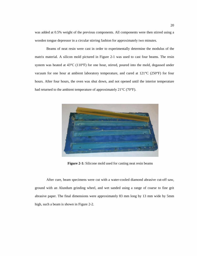
Beams of neat resin were cast in order to experimentally determine the modulus of the

matrix material. A silicon mold pictured in Figure 2-1 was used to cast four beams. The resin

system was heated at 43°C (110°F) for one hour, stirred, poured into the mold, degassed under

vacuum for one hour at ambient laboratory temperature, and cured at 121°C (250°F) for four

hours. After four hours, the oven was shut down, and not opened until the interior temperature

had returned to the ambient temperature of approximately 21°C (70°F).

Figure 2-1: Silicone mold used for casting neat resin beams

After cure, beam specimens were cut with a water-cooled diamond abrasive cut-off saw,

ground with an Alundum grinding wheel, and wet sanded using a range of coarse to fine grit

abrasive paper. The final dimensions were approximately 83 mm long by 13 mm wide by 5mm

high, such a beam is shown in Figure 2-2.

21

Figure 2-2: Neat resin specimen prepared for experimentation

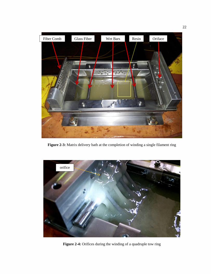
2.2 Matrix Delivery

The matrix was delivered to all fibers using an unheated stainless steel bath. The bath is

pictured in Figure 2-3. The fibers entered the bath dry, passed under three stainless steel bars that

were submerged in the matrix, picked up the resin, exited the bath, passed through the orifices

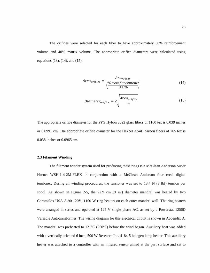
where excess resin is squeezed off, and continue to the part saturated in resin. Figure 2-4 shows

the back flow from the orifices for four tows.

22

Figure 2-3: Matrix delivery bath at the completion of winding a single filament ring

Figure 2-4: Orifices during the winding of a quadruple tow ring

Fiber Comb Glass Fiber Wet Bars Resin Oriface

orifice

23

The orifices were selected for each fiber to have approximately 60% reinforcement

volume and 40% matrix volume. The appropriate orifice diameters were calculated using

equations (13), (14), and (15).

𝐴𝑟𝑒𝑎𝑜𝑟𝑖𝑓𝑖𝑐𝑒 =

𝐴𝑟𝑒𝑎𝑓𝑖𝑏𝑒𝑟

% 𝑟𝑒𝑖𝑛𝑓𝑜𝑟𝑐𝑒𝑚𝑒𝑛𝑡100%

(14)

𝐷𝑖𝑎𝑚𝑒𝑡𝑒𝑟𝑜𝑟𝑖𝑓𝑖𝑐𝑒 = 2

𝐴𝑟𝑒𝑎𝑜𝑟𝑖𝑓𝑖𝑐𝑒𝜋

(15)

The appropriate orifice diameter for the PPG Hybon 2022 glass fibers of 1100 tex is 0.039 inches

or 0.0991 cm. The appropriate orifice diameter for the Hexcel AS4D carbon fibers of 765 tex is

0.038 inches or 0.0965 cm.

2.3 Filament Winding

The filament winder system used for producing these rings is a McClean Anderson Super

Hornet WSH-1-4-2M-FLEX in conjunction with a McClean Anderson four creel digital

tensioner. During all winding procedures, the tensioner was set to 13.4 N (3 lbf) tension per

spool. As shown in Figure 2-5, the 22.9 cm (9 in.) diameter mandrel was heated by two

Chromalox USA A-90 120V, 1100 W ring heaters on each outer mandrel wall. The ring heaters

were arranged in series and operated at 125 V single phase AC, as set by a Powerstat 1256D

Variable Autotransformer. The wiring diagram for this electrical circuit is shown in Appendix A.

The mandrel was preheated to 121°C (250°F) before the wind began. Auxiliary heat was added

with a vertically oriented 6 inch, 500 W Research Inc. 4184-5 halogen lamp heater. This auxiliary

heater was attached to a controller with an infrared sensor aimed at the part surface and set to

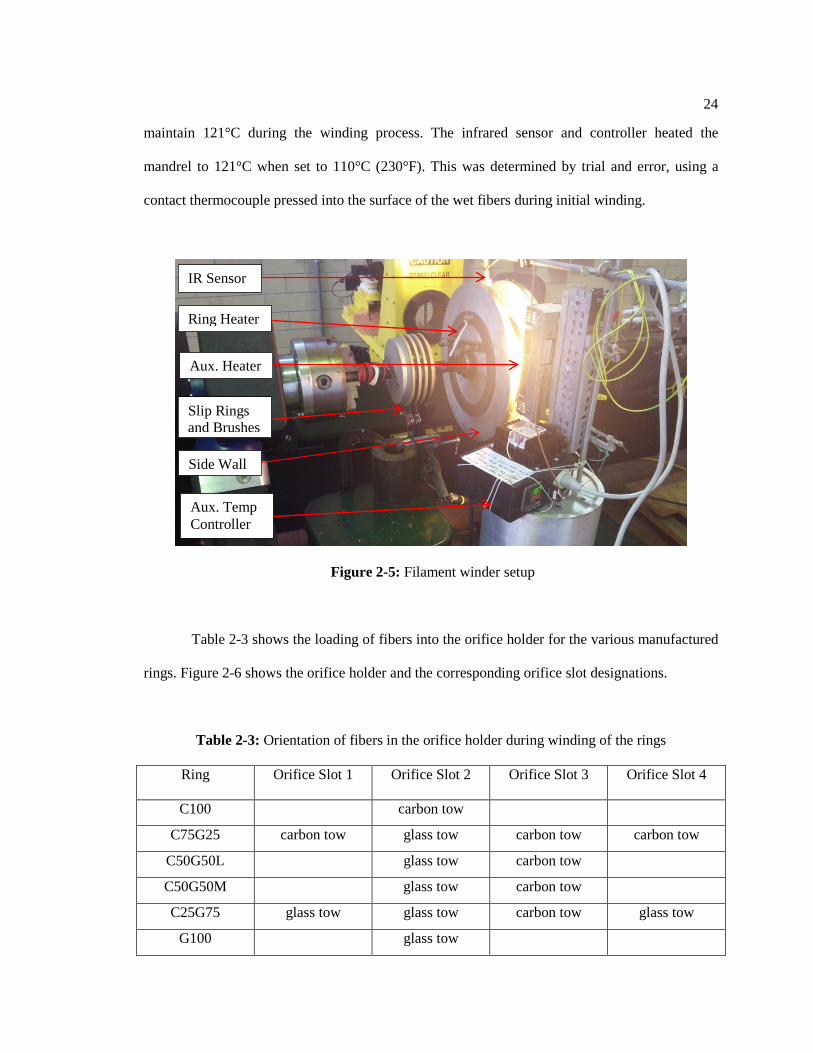
24

maintain 121°C during the winding process. The infrared sensor and controller heated the

mandrel to 121°C when set to 110°C (230°F). This was determined by trial and error, using a

contact thermocouple pressed into the surface of the wet fibers during initial winding.

Figure 2-5: Filament winder setup

Table 2-3 shows the loading of fibers into the orifice holder for the various manufactured

rings. Figure 2-6 shows the orifice holder and the corresponding orifice slot designations.

Table 2-3: Orientation of fibers in the orifice holder during winding of the rings

Ring Orifice Slot 1 Orifice Slot 2 Orifice Slot 3 Orifice Slot 4

C100 carbon tow

C75G25 carbon tow glass tow carbon tow carbon tow

C50G50L glass tow carbon tow

C50G50M glass tow carbon tow

C25G75 glass tow glass tow carbon tow glass tow

G100 glass tow

Ring Heater

Slip Rings and Brushes

IR Sensor

Aux. Heater

Aux. Temp Controller

Side Wall

25

Figure 2-6: Orifice slot designations in orifice holder

After the wind was completed, the ring was allowed to gel for 90 minutes at 121°C. The

part was transferred to a forced air oven for the final cure at 121°C. After four hours, the oven

was shut down, and was not opened until the temperature inside had returned to the ambient

temperature of approximately 21°C (70°F).

Three categories of rings were wound: single tow, double tow, and quadruple tow. Single

tow rings were wound for the two cases of C100 and G100 (100% glass and 100% carbon

reinforcement volume fraction), non-hybrid rings. Double tow rings were wound for the C50G50

cases. Quadruple tow hybrids were wound for the C25G75 and C75G25 rings. Pictured in Figure

2-7 is a quadruple tow hybrid ring during the winding process. In Figure 2-7, the fibers are

orifice #1 orifice #2 orifice #3 orifice #4

26

consolidated into one band as they were deposited onto the part surface. This consolidation is

achieved by the use of a payout eye. The payout eye is featured in Figure 2-8.

Figure 2-7: Winding of a quadruple tow ring

Figure 2-8: Four tows entering (lower right) and leaving (upper left) the payout eye

27

Table 2-4 contains the parameters used during the winding of each type of ring. The

properties were controlled as tightly as possible, and no fiber breaks occurred during the winding

of any of the tested rings.

Table 2-4: Winding parameters based on number of tows per ring

Fiber Bandwidth

(cm)

Effective Wind

Angle (°)*

Mandrel

Speed (RPM)

Spool Tension

(N)

Single Tow 0.229 ~0.18 8.75 13.4

Double Tow 0.457 ~0.36 8.75 13.4

Quadruple Tow 0.914 ~0.73 8.75 13.4

*Angle measured relative to the hoop direction

2.4 Images of Rings and Beam Specimens

Figures 2-9 to 2-14 show the cross section of each hoop wound ring. All cases of

composites tested are pictured here. These images were taken after specimens had been extracted

from the rings. None of the external surfaces have been ground or sanded on these rings. The

uneven thickness of the rings can be attributed to inaccuracies during the programing of the

winder. A low thickness indicates that the winding program was not reaching that area as much as

a section of higher thickness, due to the pattern length coordinates of the program.

28

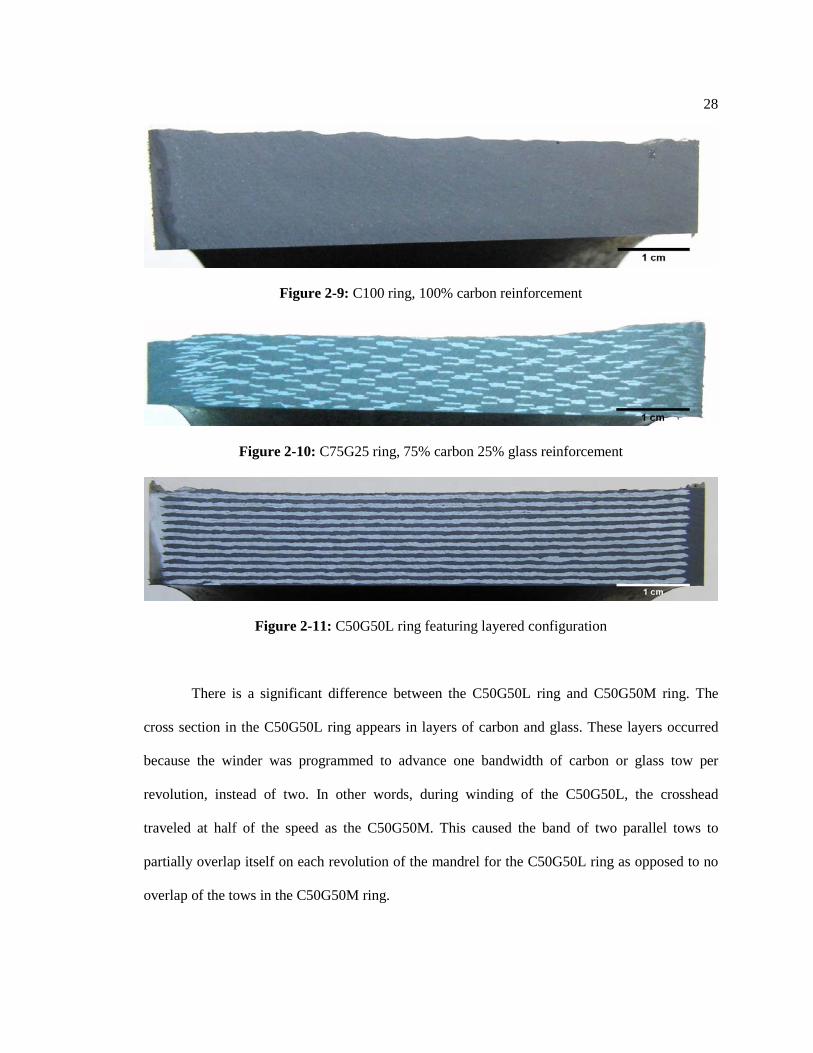
Figure 2-9: C100 ring, 100% carbon reinforcement

Figure 2-10: C75G25 ring, 75% carbon 25% glass reinforcement

Figure 2-11: C50G50L ring featuring layered configuration

There is a significant difference between the C50G50L ring and C50G50M ring. The

cross section in the C50G50L ring appears in layers of carbon and glass. These layers occurred

because the winder was programmed to advance one bandwidth of carbon or glass tow per

revolution, instead of two. In other words, during winding of the C50G50L, the crosshead

traveled at half of the speed as the C50G50M. This caused the band of two parallel tows to

partially overlap itself on each revolution of the mandrel for the C50G50L ring as opposed to no

overlap of the tows in the C50G50M ring.

29

Figure 2-12: C50G50M ring showing mixed configuration

Figure 2-13: C25G75 ring, slight moisture absorption in lower left hand corner

Figure 2-14: G100 ring

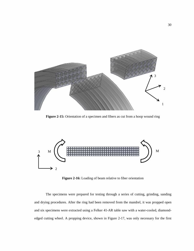
2.5 Specimen Preparation

The specimens fabricated for this investigation were cut from hoop wound rings in an

orientation that would allow measurement of the transverse properties of the nearly unidirectional

hybrid composites by means of a beam test. Figure 2-15 shows a specimen as it was cut from a

hoop wound ring. The moments were applied to the beam as shown in Figure 2-16. The

transverse modulus and strength of the material were therefore measured along the axial direction

of the ring.

30

Figure 2-15: Orientation of a specimen and fibers as cut from a hoop wound ring

Figure 2-16: Loading of beam relative to fiber orientation

The specimens were prepared for testing through a series of cutting, grinding, sanding

and drying procedures. After the ring had been removed from the mandrel, it was propped open

and six specimens were extracted using a Felker 41-AR table saw with a water-cooled, diamond-

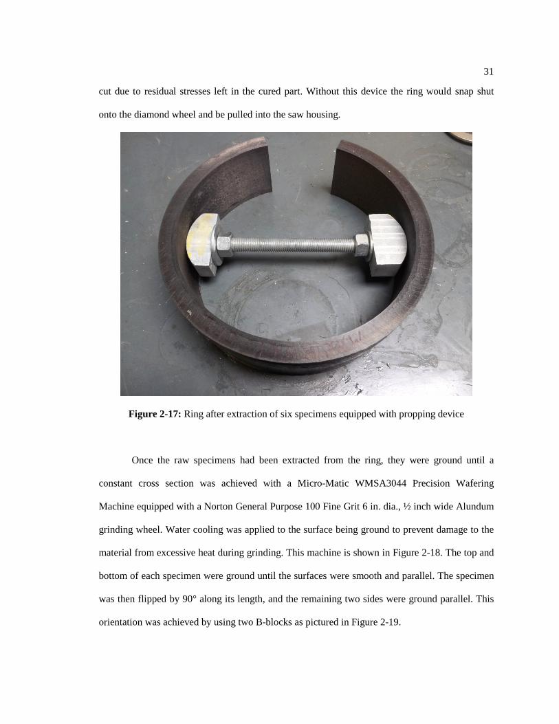
edged cutting wheel. A propping device, shown in Figure 2-17, was only necessary for the first

1

2

3

2

3

M M

31

cut due to residual stresses left in the cured part. Without this device the ring would snap shut

onto the diamond wheel and be pulled into the saw housing.

Figure 2-17: Ring after extraction of six specimens equipped with propping device

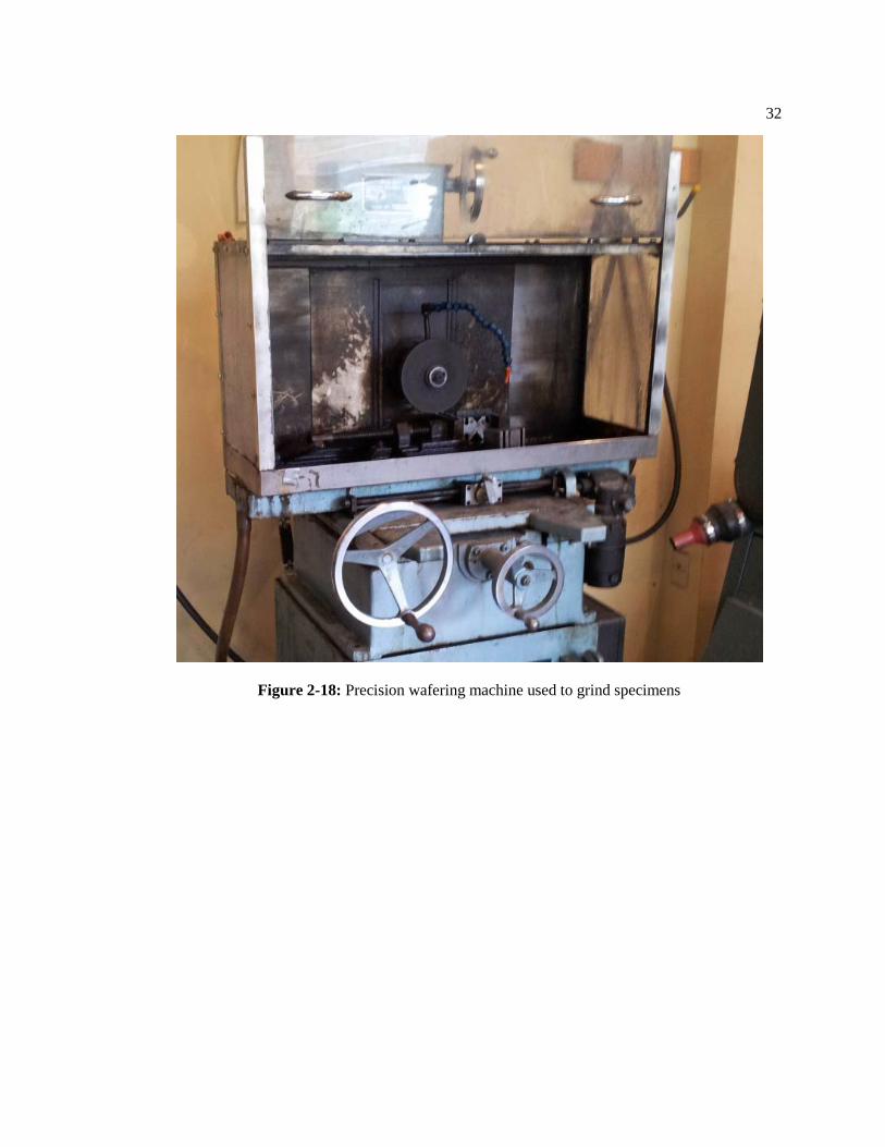
Once the raw specimens had been extracted from the ring, they were ground until a

constant cross section was achieved with a Micro-Matic WMSA3044 Precision Wafering

Machine equipped with a Norton General Purpose 100 Fine Grit 6 in. dia., ½ inch wide Alundum

grinding wheel. Water cooling was applied to the surface being ground to prevent damage to the

material from excessive heat during grinding. This machine is shown in Figure 2-18. The top and

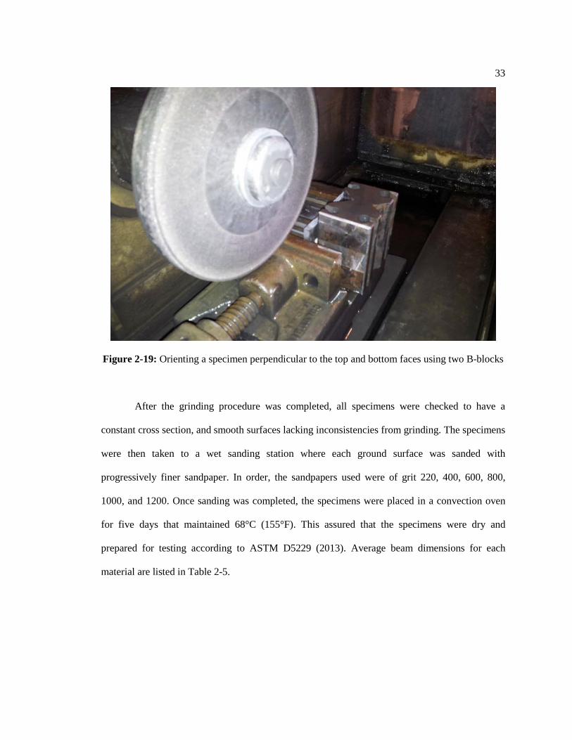
bottom of each specimen were ground until the surfaces were smooth and parallel. The specimen

was then flipped by 90° along its length, and the remaining two sides were ground parallel. This

orientation was achieved by using two B-blocks as pictured in Figure 2-19.

32

Figure 2-18: Precision wafering machine used to grind specimens

33

Figure 2-19: Orienting a specimen perpendicular to the top and bottom faces using two B-blocks

After the grinding procedure was completed, all specimens were checked to have a

constant cross section, and smooth surfaces lacking inconsistencies from grinding. The specimens

were then taken to a wet sanding station where each ground surface was sanded with

progressively finer sandpaper. In order, the sandpapers used were of grit 220, 400, 600, 800,

1000, and 1200. Once sanding was completed, the specimens were placed in a convection oven

for five days that maintained 68°C (155°F). This assured that the specimens were dry and

prepared for testing according to ASTM D5229 (2013). Average beam dimensions for each

material are listed in Table 2-5.

34

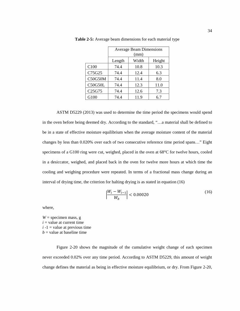
Table 2-5: Average beam dimensions for each material type

Average Beam Dimensions (mm)

Length Width Height

C100 74.4 10.8 10.3 C75G25 74.4 12.4 6.3 C50G50M 74.4 11.4 8.0 C50G50L 74.4 12.3 11.0 C25G75 74.4 12.6 7.3 G100 74.4 11.9 6.7

ASTM D5229 (2013) was used to determine the time period the specimens would spend

in the oven before being deemed dry. According to the standard, “…a material shall be defined to

be in a state of effective moisture equilibrium when the average moisture content of the material

changes by less than 0.020% over each of two consecutive reference time period spans…” Eight

specimens of a G100 ring were cut, weighed, placed in the oven at 68°C for twelve hours, cooled

in a desiccator, weighed, and placed back in the oven for twelve more hours at which time the

cooling and weighing procedure were repeated. In terms of a fractional mass change during an

interval of drying time, the criterion for halting drying is as stated in equation (16)

𝑊𝑖 −𝑊𝑖−1

𝑊𝑏 < 0.00020 (16)

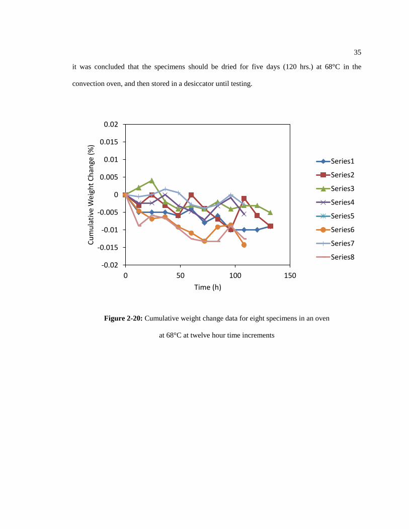
where, W = specimen mass, g i = value at current time i -1 = value at previous time b = value at baseline time Figure 2-20 shows the magnitude of the cumulative weight change of each specimen

never exceeded 0.02% over any time period. According to ASTM D5229, this amount of weight

change defines the material as being in effective moisture equilibrium, or dry. From Figure 2-20,

35

it was concluded that the specimens should be dried for five days (120 hrs.) at 68°C in the

convection oven, and then stored in a desiccator until testing.

Figure 2-20: Cumulative weight change data for eight specimens in an oven

at 68°C at twelve hour time increments

-0.02

-0.015

-0.01

-0.005

0

0.005

0.01

0.015

0.02

0 50 100 150

Cum

ulat

ive

Wei

ght C

hang

e (%

)

Time (h)

Series1

Series2

Series3

Series4

Series5

Series6

Series7

Series8

36

Chapter 3

Test Methods

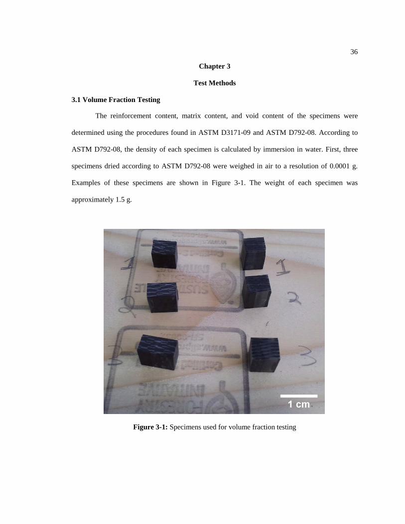
3.1 Volume Fraction Testing

The reinforcement content, matrix content, and void content of the specimens were

determined using the procedures found in ASTM D3171-09 and ASTM D792-08. According to

ASTM D792-08, the density of each specimen is calculated by immersion in water. First, three

specimens dried according to ASTM D792-08 were weighed in air to a resolution of 0.0001 g.

Examples of these specimens are shown in Figure 3-1. The weight of each specimen was

approximately 1.5 g.

Figure 3-1: Specimens used for volume fraction testing

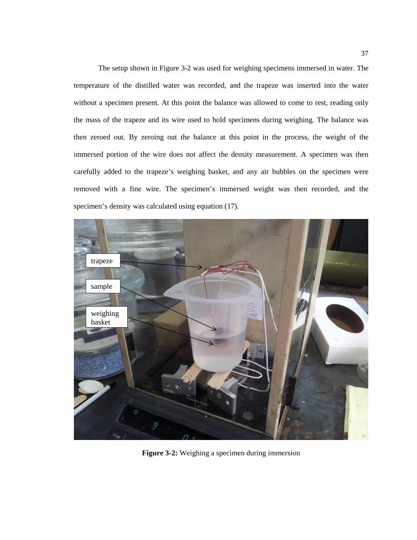
37

The setup shown in Figure 3-2 was used for weighing specimens immersed in water. The

temperature of the distilled water was recorded, and the trapeze was inserted into the water

without a specimen present. At this point the balance was allowed to come to rest, reading only

the mass of the trapeze and its wire used to hold specimens during weighing. The balance was

then zeroed out. By zeroing out the balance at this point in the process, the weight of the

immersed portion of the wire does not affect the density measurement. A specimen was then

carefully added to the trapeze’s weighing basket, and any air bubbles on the specimen were

removed with a fine wire. The specimen’s immersed weight was then recorded, and the

specimen’s density was calculated using equation (17).

Figure 3-2: Weighing a specimen during immersion

trapeze

sample

weighing basket

38

𝜌specimen =𝑚dry

𝑚dry − 𝑚immersed𝜌water @ temp

(17)

where,

mdry: mass of the dry specimen mimmersed: mass of the specimen during immersion ρwater @ temp: density of water at the measured temperature ρspecimen: density of the specimen

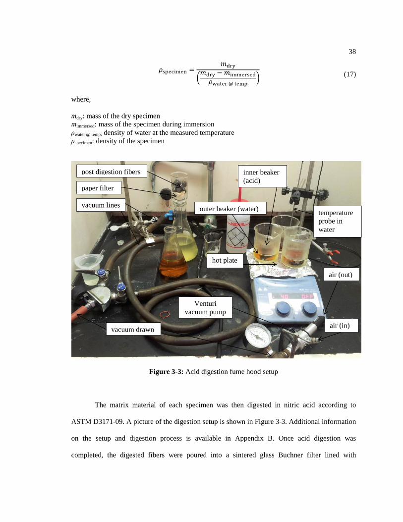
Figure 3-3: Acid digestion fume hood setup

The matrix material of each specimen was then digested in nitric acid according to

ASTM D3171-09. A picture of the digestion setup is shown in Figure 3-3. Additional information

on the setup and digestion process is available in Appendix B. Once acid digestion was

completed, the digested fibers were poured into a sintered glass Buchner filter lined with

post digestion fibers

paper filter

vacuum lines outer beaker (water)

inner beaker (acid)

hot plate

air (in)

air (out)

Venturi vacuum pump

vacuum drawn

temperature probe in water

39

Whatman 1006-150 filter paper of diameter 150 mm. The acid was then pulled through the filter

under vacuum of approximately 60 kPa. This vacuum was achieved by attaching an air supply of

414 kPa (60 psig) to the Venturi vacuum pump. The filter was then transferred to another vacuum

beaker where it washed three times with 40 mL of distilled water and washed once with 40 mL of

acetone to assist with drying. Finally, the filter was transferred to an oven where it was dried for

one hour at 100°C (212°F), cooled in a desiccator, and then immediately weighed. The following

equations from ASTM D3171-09 were used to determine reinforcement content by volume (18),

matrix content by volume (19), and void content by volume (20).

𝑉𝑟 =

𝑀𝑓

𝑀𝑖

𝜌𝑐𝜌𝑟∙ 100% (18)

𝑉𝑚 =

𝑀𝑖 −𝑀𝑓

𝑀𝑖

𝜌𝑐𝜌𝑚

∙ 100% (19)

𝑉𝑣 = 100− (𝑉𝑟 + 𝑉𝑚)

(20)

where,

Vr: volume fraction of reinforcement (%) Vm: volume fraction of matrix (%) Vv: void volume fraction (%) Mf: mass of fibers Mi: initial specimen mass ρc: specimen density, specimen densities are listed in Table 4-2 ρr: reinforcement density, reinforcement densities are listed in Table 2-1 ρm : matrix density, experimental matrix density is listed in Table 4-2 In the case of the hybrid specimens, the fiber volume fraction required a modified

equation for reinforcement content, and combustion testing was used to verify fiber content

proportions used with that modified version of the equation. The modified version of equation

(18) is shown below, (21), solved for the volume fraction of carbon in a hybrid specimen.

Equation (22) is used to determine the mass of carbon fiber in a hybrid specimen of known total

mass:

40

𝑉𝑟,𝑐 =

𝑀𝑓,𝑐

𝑀𝑖

𝜌𝑐𝜌𝑟,𝑐

∙ 100% (21)

𝑀𝑓,𝑐 = 𝑀𝑓𝑁𝑐𝑇𝑐

(𝑁𝑐𝑇𝑐 + 𝑁𝑔𝑇𝑔) (22)

where,

Mf,c: mass of carbon fibers present (g) Vr,c: volume fraction of carbon reinforcement in sample (%) Nc/g: number of tows of carbon or glass Tc/g: tex of carbon or glass tow (g/m) The modified version of equation (18) is shown below (23) solved for the volume fraction of

glass in a hybrid specimen. Equation (24) is used to determine the mass of glass fiber in a hybrid

specimen of known total mass.

𝑉𝑟,𝑔 =

𝑀𝑓,𝑔

𝑀𝑖

𝜌𝑔𝜌𝑟,𝑔

∙ 100% (23)

𝑀𝑓,𝑔 = 𝑀𝑓

𝑁𝑔𝑇𝑔(𝑁𝑐𝑇𝑐 + 𝑁𝑔𝑇𝑔)

(24)

As an example, in a C25G75 ring, one tow of carbon fiber (Nc = 1) and three tows of

glass fiber (Ng = 3) are used to calculate the mass of carbon in a hybrid specimen. As a

verification test, the digested hybrid specimens of C50G50L and C50G50M were combusted

according to ASTM D3171-09 at 800°C and compared to the results of equations (22) and (24).

The results and comparisons from three specimens of C50G50M and three specimens of

C50G50L are tabulated in Table 3-1, where the percent difference between the methods was

calculated according to equation (25)

41

Table 3-1: Comparison of mass fraction results from combustion testing and

equations (22) and (24)

Carbon Mass (g)

Glass Mass (g)

Calculated using (22) and (24) 0.4101 0.5898 Combustion Testing 0.4060 0.5939 % Difference -1.0 0.7

𝐷𝑖𝑓𝑓𝑒𝑟𝑒𝑛𝑐𝑒 (%) =

(𝐶𝑜𝑚𝑏𝑢𝑠𝑡𝑖𝑜𝑛 − 𝐶𝑎𝑙𝑐𝑢𝑙𝑎𝑡𝑒𝑑)𝐶𝑎𝑙𝑐𝑢𝑙𝑎𝑡𝑒𝑑

∙ 100%

(25)

The amount of error shown in Table 3-1 was determined to be acceptable, and the mass

fractions of carbon and glass fibers were calculated using equations (22) and (24) for the

constituent content calculations of hybrid specimens.

3.2 Four Point Flexure Testing

Four point flexure testing following ASTM D6272 (2013) was used to test the specimens

mechanically to failure. This test method was chosen because it provides a constant moment

across the middle span of the composite. The positions of the rollers are shown in Figure 3-4. One

exception to the standard was the use of an L/5 shear arm as opposed to an L/4 shear arm. This

change was done to allow sufficient clearance between the top rollers and the extensometer

located on the bottom of the beam. For all tests, the values of L, 3L/5, and L/5, were set to 54.61

mm, 32.77 mm, and 10.92 mm, respectively.

42

Figure 3-4: Four point flexure setup labeled with spans

The tests were conducted on a Tinius Olsen Electomatic 267kN (60,000 lb) screw-driven

load frame. Strain was measured on the tensile face of the specimen with an Epsilon Technology

Corp. 3442-0050- 010-LHT strain-gage based extensometer of gage length 9.525 mm (0.375 in.).

The lowest load range of 10.675 kN (2400 lb) was selected for the tests since failure typically

occurred at approximately 1.33 kN (300 lb). The load and extension were recorded using a

National Instruments SCB-68 digital acquisition board. The extensometer was attached to a

Vishay Measurements Group 2120A Strain Gage Conditioner. Before each series of tests, the

extensometer was calibrated over at least twice the range of predicted extension using a

micrometer attached to an aluminum base for accuracy. The test setup is shown in Figure 3-5.

L/5

L

3L/5

43

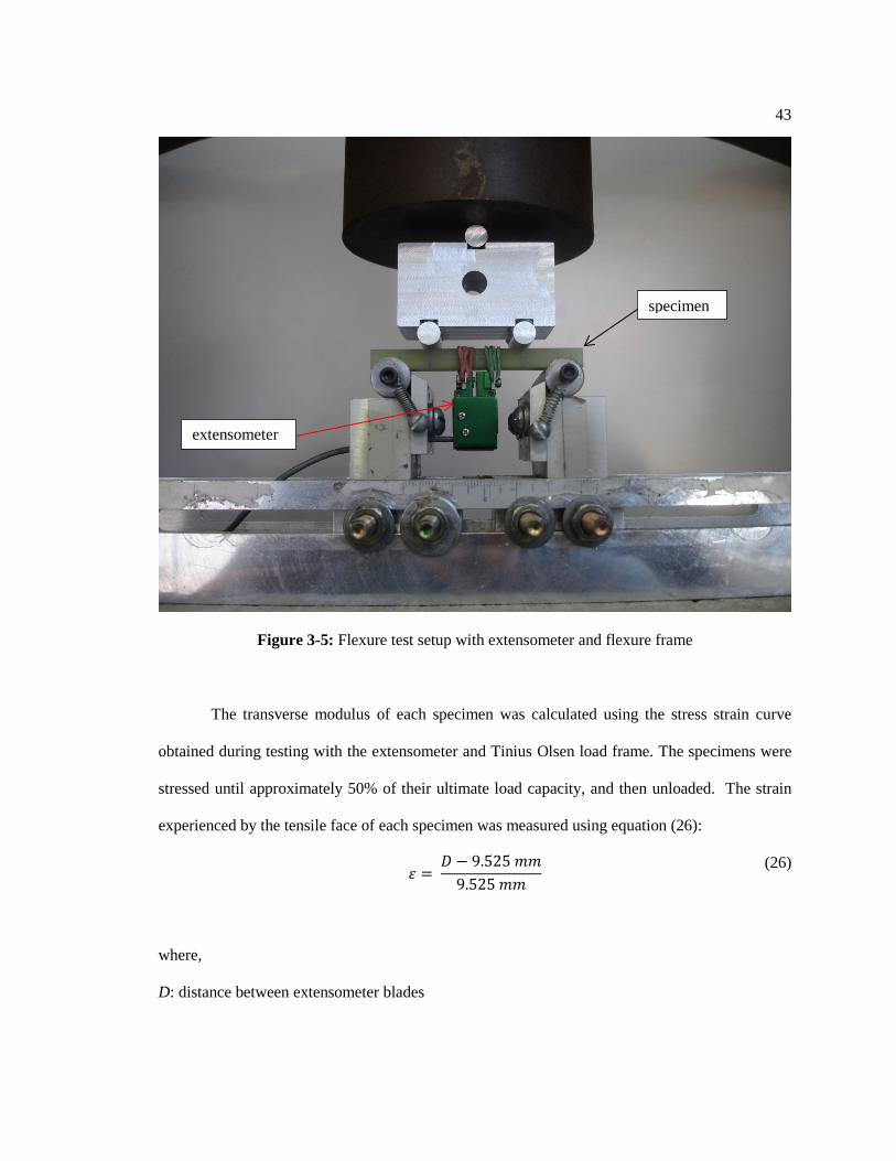
Figure 3-5: Flexure test setup with extensometer and flexure frame

The transverse modulus of each specimen was calculated using the stress strain curve

obtained during testing with the extensometer and Tinius Olsen load frame. The specimens were

stressed until approximately 50% of their ultimate load capacity, and then unloaded. The strain

experienced by the tensile face of each specimen was measured using equation (26):

𝜀 =

𝐷 − 9.525 𝑚𝑚9.525 𝑚𝑚

(26)

where,

D: distance between extensometer blades

extensometer

specimen

44

The stress in each specimen was determined using equation (27) for four point flexure in an L/5

load span:

𝜎 = 3𝑃𝐿5𝑏ℎ2

(27)

where,

P: applied load L: width of outer support span b: width of specimen h: height of specimen Knowing the stress from equation (27), and the strain from the extensometer, equation (28) was

used to determine the transverse modulus of each specimen:

𝐸2 = 𝜎50% − 𝜎25%𝜀50% − 𝜀25%

(28)

where,

σx%: stress at x% of the estimated load capacity of the specimen εx%: strain at the corresponding x% stress The extensometer was detached during failure testing to prevent damage to the device during

fracture of the specimen.

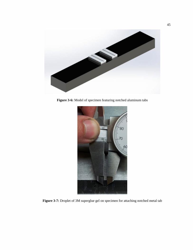
During initial testing, slippage of the extensometer knife edges in direct contact with the

specimen was detected. Therefore, v-notched aluminum tabs of approximate size 10mm × 5mm ×

2mm were attached to the specimens using 3M brand superglue gel (Figure 3-6). The droplet of

glue was of minimal size, not to exceed 0.254 cm (0.1 in.) in diameter as pictured in Figure 3-7.

The blades of the extensomer were firmly positioned inside the v-notches of the tabs. To aid in

the positioning of the aluminum tabs and rollers during testing, a laser etched polycarbonate sheet

was used to mark each specimen with reference lines as pictured in Figure 3-8. Two notched tabs

were then quickly applied and aligned with the extensometer slots perpendicular to the length of

the specimen as shown in Figure 3-9.

45

Figure 3-6: Model of specimen featuring notched aluminum tabs

Figure 3-7: Droplet of 3M superglue gel on specimen for attaching notched metal tab

46

Figure 3-8: Laser etched polycarbonate sheet being used to mark specimen

Figure 3-9: Alignment of notched tabs using aluminum alignment blocks

The alignment procedure shown in Figure 3-9 was used to ensure the extensometer

measurement to be parallel to the length of the specimen. The aluminum block which directly

contacts the v-notched tabs was CNC machined to be an exact replica to 0.00254 cm (0.001”) of

the extensometer used during testing. The use of this block minimizes the chance of damage to

the extensometer during handling and prevents undesired outward slippage of the notched tabs

during the application of vertical load. A force of approximately 5 N was applied vertically

downward to block #2 for five seconds to set the notched tabs into place. Block #1 was held in

firm contact with the specimen as shown in Figure 3-6 during the entire process. Block #2’s rear

block #1

block #2

47

face was parallel to block #1’s front face as shown in Figure 3-9 while the vertical load was

applied. In turn, this block also helps assure that the initial separation of the notched tabs and

extensometer knife edges is virtually the same for all specimens. Starting the extensometer from

nearly the same position on each specimen is intended to increase precision among data collected.

The potential additional reinforcement of the notched tabs and adhesive was considered

during the testing process, so a control experiment was run without the tabs. In the control

experiment, Vishay Micro-Measurements CEA-06-125UN-120 strain gages were attached to the

top and bottom of a G100 specimen. Based on these measurements and assumptions of pure

bending and a material having unequal elastic moduli in tension and compression, the following

analysis was carried out to determine the two moduli (Henry, 2011).

In a material with unequal tensile and compressive moduli, the strain varies linearly

through the depth of the beam and the stress varies bilinearly, as pictured in Figure 3-10. The

neutral axis position is denoted zna. The following derivation of stresses at the top and bottom of

the beam was provided by Henry (2011).

Figure 3-10: Assumed stress and strain distributions in a bimodular beam in pure bending

(Henry, 2011)

Relating ε, z, d, εT, and εC using similar triangles leads to equation (29)

ε = 0 σ = 0

48

𝜀 = 𝜀𝑇 − (𝜀𝑇 − 𝜀𝐶)

𝑑𝑧 (29)

where,

ε: strain z: vertical distance defined in Figure 3-7 d: beam depth as defined in Figure 3-7 εT: maximum tensile strain as defined in Figure 3-7 εC: maximum compressive strain as defined in Figure 3-7

Evaluating equation (29) with ε = 0 to find an expression for the neutral axis position, z = zNA,

yields equation (30).

𝑧𝑁𝐴 =

𝑑𝜀𝑇𝜀𝑇 − 𝜀𝐶

(30)

In equation (30) the only unknown is zNA since εT and εC are measured during the testing

procedure and d is the specimen thickness. The force resultants of the two triangular stress

distributions must balance each other for axial equilibrium. The force balance yields equation

(31).

12𝜎𝑡𝑧𝑁𝐴 =

12𝜎𝑐(𝑑 − 𝑧𝑁𝐴) (31)

Equation (31) can be rearranged into equation (32).

𝜎𝑐𝜎𝑡

= 𝑧𝑁𝐴

𝑑 − 𝑧𝑁𝐴 (32)

The moment due to the triangular stress distributions must equal the applied moment shown in

Figure 3-11.

49

Figure 3-11: Moment balance in a bimodular material (Henry, 2011)

The resultant forces are described by equations (33a) and (33b),

𝐹𝑐 = 12

(𝑑 − 𝑧𝑁𝐴)𝑏𝜎𝑐 (33a)

𝐹𝑡 = 12𝑧𝑁𝐴𝑏𝜎𝑡 (33b)

where b is the specimen width. The moment applied in a four-point bending test as shown in

Figure 3-1 is PL/10, where P is the total applied load on the beam. The moment balance is

described by equation (34).

𝑀 =𝑃𝐿10

=23𝐹𝑐(𝑑 − 𝑧𝑁𝐴) +

23𝐹𝑇(𝑧𝑁𝐴) (34)

Substituting equations (33a) and (33b) into equation (34) yields a second relationship between σT

and σc shown as equation (35).

3𝑃𝐿10𝑏

= (𝑑 − 𝑧𝑁𝐴)2𝜎𝑐 + 𝑧𝑁𝐴2 𝜎𝑇 (35)

Using equation (32), equation (35) may be solved for σT.

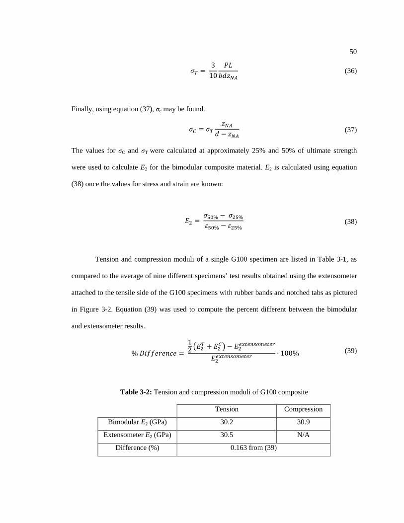
50

𝜎𝑇 = 3

10𝑃𝐿

𝑏𝑑𝑧𝑁𝐴 (36)

Finally, using equation (37), σc may be found.

𝜎𝐶 = 𝜎𝑇𝑧𝑁𝐴

𝑑 − 𝑧𝑁𝐴 (37)

The values for σC and σT were calculated at approximately 25% and 50% of ultimate strength

were used to calculate E2 for the bimodular composite material. E2 is calculated using equation

(38) once the values for stress and strain are known:

𝐸2 = 𝜎50% − 𝜎25%𝜀50% − 𝜀25%

(38)

Tension and compression moduli of a single G100 specimen are listed in Table 3-1, as

compared to the average of nine different specimens’ test results obtained using the extensometer

attached to the tensile side of the G100 specimens with rubber bands and notched tabs as pictured

in Figure 3-2. Equation (39) was used to compute the percent different between the bimodular

and extensometer results.

% 𝐷𝑖𝑓𝑓𝑒𝑟𝑒𝑛𝑐𝑒 =

12 𝐸2

𝑇 + 𝐸2𝐶 − 𝐸2𝑒𝑥𝑡𝑒𝑛𝑠𝑜𝑚𝑒𝑡𝑒𝑟

𝐸2𝑒𝑥𝑡𝑒𝑛𝑠𝑜𝑚𝑒𝑡𝑒𝑟 ∙ 100% (39)

Table 3-2: Tension and compression moduli of G100 composite

Tension Compression

Bimodular E2 (GPa) 30.2 30.9

Extensometer E2 (GPa) 30.5 N/A

Difference (%) 0.163 from (39)

51

The stress strain curve obtained using the extensometer and notched tabs on a G100

specimen is shown in Figure 3-12. The stress strain curves obtained using the strain gages and

bimodular material calculations are compared to the extensometer in Figure 3-13. From this data

and the results from Table 3-2, it was concluded that using the extensometer with notched tabs

bonded to the tensile side of the specimen is an accurate test method.

Figure 3-12: Stress strain curve of a G100 beam obtained using extensometer

0

10

20

30

40

50

60

0 0.0005 0.001 0.0015 0.002

Stre

ss (M

Pa)

Strain (ε)

Approximate 50% Load

Approximate 25% Load

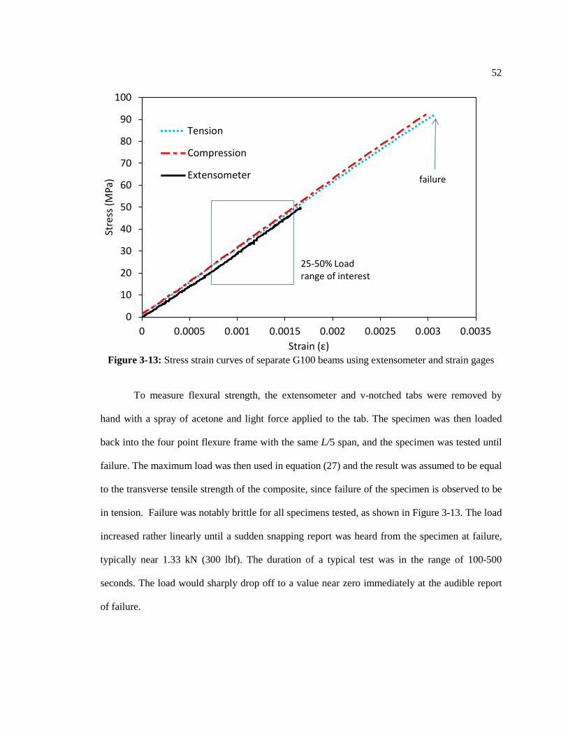
52

Figure 3-13: Stress strain curves of separate G100 beams using extensometer and strain gages

To measure flexural strength, the extensometer and v-notched tabs were removed by

hand with a spray of acetone and light force applied to the tab. The specimen was then loaded

back into the four point flexure frame with the same L/5 span, and the specimen was tested until

failure. The maximum load was then used in equation (27) and the result was assumed to be equal

to the transverse tensile strength of the composite, since failure of the specimen is observed to be

in tension. Failure was notably brittle for all specimens tested, as shown in Figure 3-13. The load

increased rather linearly until a sudden snapping report was heard from the specimen at failure,

typically near 1.33 kN (300 lbf). The duration of a typical test was in the range of 100-500

seconds. The load would sharply drop off to a value near zero immediately at the audible report

of failure.

0

10

20

30

40

50

60

70

80

90

100

0 0.0005 0.001 0.0015 0.002 0.0025 0.003 0.0035

Stre

ss (M

Pa)

Strain (ε)

Tension

Compression

Extensometer

25-50% Load range of interest

failure

53

Chapter 4

Results

4.1 Volume Fraction Data

Table 4-1 shows the average density monotonically increasing with increasing glass

reinforcement content as expected. For each specimen this data represents the average of three

individual samples. The standard deviations are all under one hundredth of a gram per cubic

centimeter.

Table 4-1: Experimentally determined densities of specimens and matrix material

Specimen Average ρ (g/cc) Standard Deviation

(g/cc) CV (%)

C100 1.5611 0.00587 0.376 C75G25 1.7349 0.00740 0.426

C50G50M 1.8816 0.00773 0.411 C50G50L 1.8699 0.00679 0.363 C25G75 1.9980 0.00921 0.461

G100 2.2541 7.54E-5 0.003 Neat Resin 1.1963 0.00251 0.210

The average volume fraction results of three specimens of each composite type are

summarized in Table 4-2. Additional statistics supporting Table 4-2 are provided in Tables 4-3

and 4-4. Appendix C contains volume fraction results from individual specimens. Originally,

reinforcement volume fraction was intended to be 60%, but it was actually closer to 70%,

presumably due to drip-off during winding. In the case of the G100 ring, the volume fraction was

considerably higher than any of the other rings.

54

Table 4-2: Summary of constituent content of rings by volume fraction percentage

Specimen Type Vr (%) Vc (%) Vg (%) Vm (%) Vv (%)

C100 68.8 68.8 0 27.5 3.72 C75G25 71.2 53.6 17.6 26.3 2.47

C50G50L 70.1 35.3 34.8 27.4 2.51 C50G50M 69.8 35.2 34.6 28.9 1.28 C25G75 69.3 17.6 51.8 27.4 3.25

G100 76.1 0 76.1 21.9 2.00

The standard deviations of reinforcement volume fraction never exceeded one percent.

The highest CV was 1.3 % for the C75G25 samples. Notice the similar reinforcement content

between C50G50L and C50G50M specimens.

Table 4-3: Reinforcement volume fraction statistics

Specimen Type Vr (%) Standard Deviation (%)

CV (%)

C100 68.8 0.25 0.37

C75G25 71.2 0.95 1.3

C50G50L 70.1 0.11 0.16

C50G50M 69.8 0.51 0.73

C25G75 69.3 0.32 0.46

G100 76.1 0.067 0.088

Void volume fraction was determined to be acceptable for all specimens. The highest

void volume fraction was found to be in the C100 specimens and C25G75 specimens. The lowest

void volume fraction was found to be in the C50G50M specimens.

55

Table 4-4: Void volume fraction statistics

Specimen Type

Vv (%) Standard Deviation

CV (%)

C100 3.72 0.37 9.7

C75G25 2.47 0.75 30

C50G50L 2.51 0.52 21

C50G50M 1.28 0.22 17

C25G75 3.25 0.73 23

G100 2.00 0.081 4.1

4.2 Beam Test Results

In Figures 4-1 to 4-6, specimens that were cut from rings, ground, sanded, dried, and

tested to failure are pictured. In all cases, failure was due to a crack that began at the tensile side

of the beam and extended almost entirely through the depth of the beam. The cracks are indicated

with arrows in Figures 4-1 to 4-6 and are most evident in Figures 4-2 and 4-3. After polishing it

was difficult to discern the different regions of carbon and E-glass with the naked eye.

Figure 4-1: C100 specimen after testing to failure

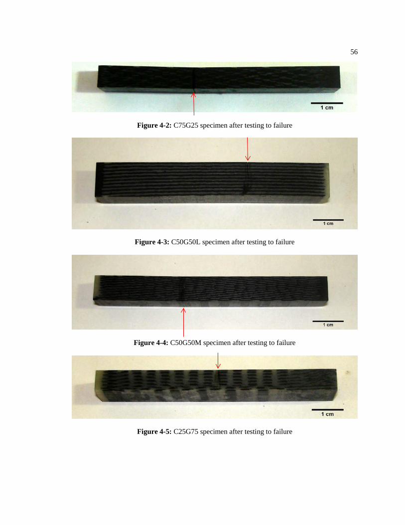
56

Figure 4-2: C75G25 specimen after testing to failure

Figure 4-3: C50G50L specimen after testing to failure

Figure 4-4: C50G50M specimen after testing to failure

Figure 4-5: C25G75 specimen after testing to failure

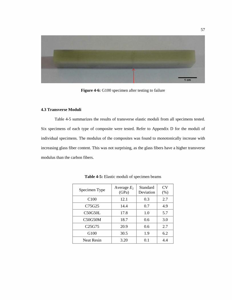
57

Figure 4-6: G100 specimen after testing to failure

4.3 Transverse Moduli

Table 4-5 summarizes the results of transverse elastic moduli from all specimens tested.

Six specimens of each type of composite were tested. Refer to Appendix D for the moduli of

individual specimens. The modulus of the composites was found to monotonically increase with

increasing glass fiber content. This was not surprising, as the glass fibers have a higher transverse

modulus than the carbon fibers.

Table 4-5: Elastic moduli of specimen beams

Specimen Type Average E2 (GPa)

Standard Deviation

CV (%)

C100 12.1 0.3 2.7 C75G25 14.4 0.7 4.9

C50G50L 17.8 1.0 5.7 C50G50M 18.7 0.6 3.0 C25G75 20.9 0.6 2.7

G100 30.5 1.9 6.2 Neat Resin 3.20 0.1 4.4

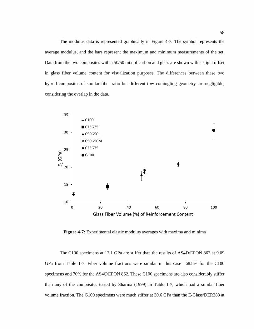
58

The modulus data is represented graphically in Figure 4-7. The symbol represents the

average modulus, and the bars represent the maximum and minimum measurements of the set.

Data from the two composites with a 50/50 mix of carbon and glass are shown with a slight offset

in glass fiber volume content for visualization purposes. The differences between these two

hybrid composites of similar fiber ratio but different tow comingling geometry are negligible,

considering the overlap in the data.

Figure 4-7: Experimental elastic modulus averages with maxima and minima

The C100 specimens at 12.1 GPa are stiffer than the results of AS4D/EPON 862 at 9.09

GPa from Table 1-7. Fiber volume fractions were similar in this case—68.8% for the C100

specimens and 70% for the AS4C/EPON 862. These C100 specimens are also considerably stiffer

than any of the composites tested by Sharma (1999) in Table 1-7, which had a similar fiber

volume fraction. The G100 specimens were much stiffer at 30.6 GPa than the E-Glass/DER383 at

10

15

20

25

30

35

0 20 40 60 80 100

E 2 (G

Pa)

Glass Fiber Volume (%) of Reinforcement Content

C100

C75G25

C50G50L

C50G50M

C25G75

G100

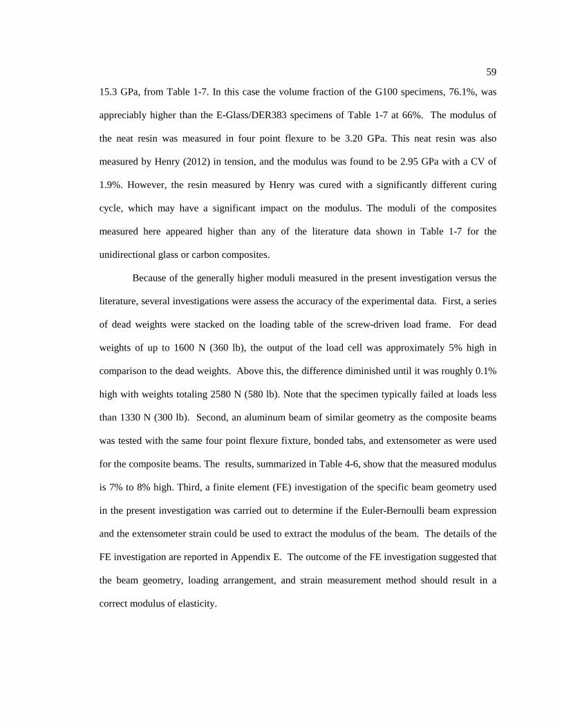
59

15.3 GPa, from Table 1-7. In this case the volume fraction of the G100 specimens, 76.1%, was

appreciably higher than the E-Glass/DER383 specimens of Table 1-7 at 66%. The modulus of

the neat resin was measured in four point flexure to be 3.20 GPa. This neat resin was also

measured by Henry (2012) in tension, and the modulus was found to be 2.95 GPa with a CV of

1.9%. However, the resin measured by Henry was cured with a significantly different curing

cycle, which may have a significant impact on the modulus. The moduli of the composites

measured here appeared higher than any of the literature data shown in Table 1-7 for the

unidirectional glass or carbon composites.

Because of the generally higher moduli measured in the present investigation versus the

literature, several investigations were assess the accuracy of the experimental data. First, a series

of dead weights were stacked on the loading table of the screw-driven load frame. For dead

weights of up to 1600 N (360 lb), the output of the load cell was approximately 5% high in

comparison to the dead weights. Above this, the difference diminished until it was roughly 0.1%

high with weights totaling 2580 N (580 lb). Note that the specimen typically failed at loads less

than 1330 N (300 lb). Second, an aluminum beam of similar geometry as the composite beams

was tested with the same four point flexure fixture, bonded tabs, and extensometer as were used

for the composite beams. The results, summarized in Table 4-6, show that the measured modulus

is 7% to 8% high. Third, a finite element (FE) investigation of the specific beam geometry used

in the present investigation was carried out to determine if the Euler-Bernoulli beam expression

and the extensometer strain could be used to extract the modulus of the beam. The details of the

FE investigation are reported in Appendix E. The outcome of the FE investigation suggested that

the beam geometry, loading arrangement, and strain measurement method should result in a

correct modulus of elasticity.

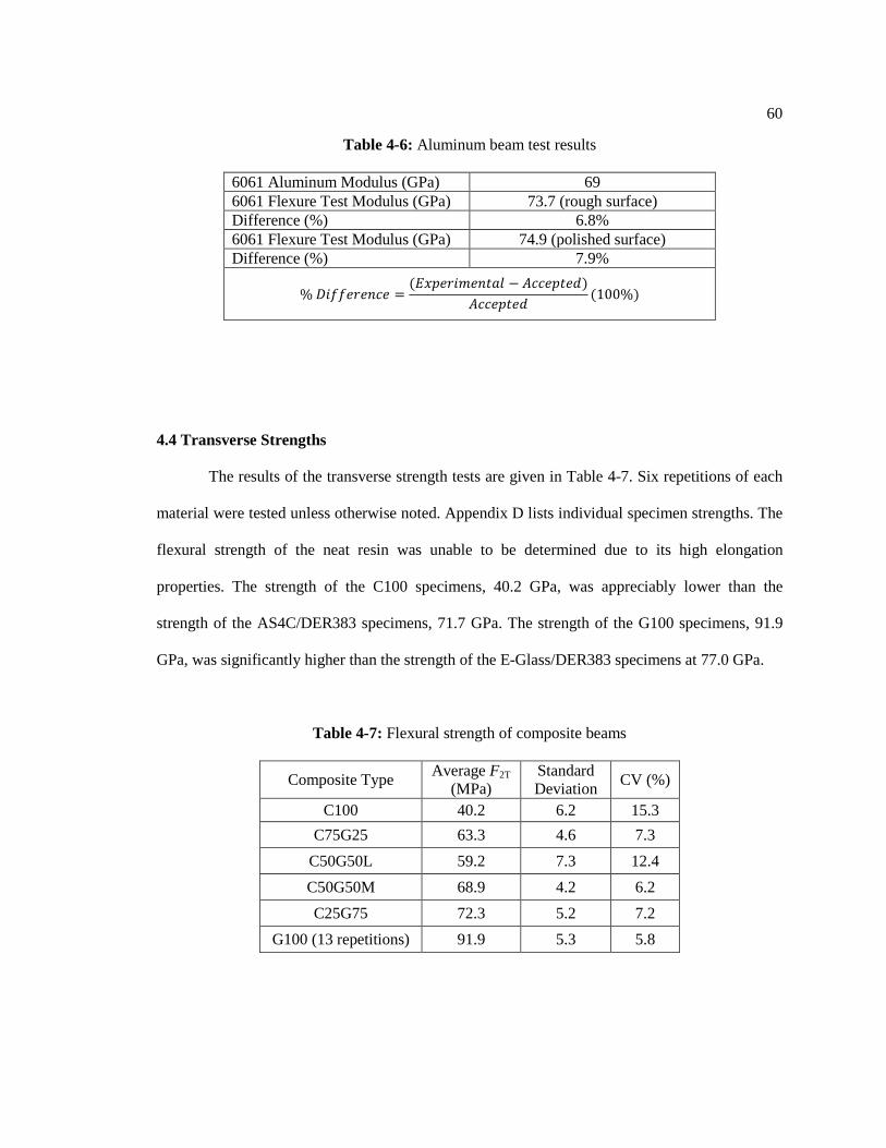
60

Table 4-6: Aluminum beam test results

6061 Aluminum Modulus (GPa) 69 6061 Flexure Test Modulus (GPa) 73.7 (rough surface) Difference (%) 6.8% 6061 Flexure Test Modulus (GPa) 74.9 (polished surface) Difference (%) 7.9%

% 𝐷𝑖𝑓𝑓𝑒𝑟𝑒𝑛𝑐𝑒 =(𝐸𝑥𝑝𝑒𝑟𝑖𝑚𝑒𝑛𝑡𝑎𝑙 − 𝐴𝑐𝑐𝑒𝑝𝑡𝑒𝑑)

𝐴𝑐𝑐𝑒𝑝𝑡𝑒𝑑(100%)

4.4 Transverse Strengths

The results of the transverse strength tests are given in Table 4-7. Six repetitions of each

material were tested unless otherwise noted. Appendix D lists individual specimen strengths. The

flexural strength of the neat resin was unable to be determined due to its high elongation

properties. The strength of the C100 specimens, 40.2 GPa, was appreciably lower than the

strength of the AS4C/DER383 specimens, 71.7 GPa. The strength of the G100 specimens, 91.9

GPa, was significantly higher than the strength of the E-Glass/DER383 specimens at 77.0 GPa.

Table 4-7: Flexural strength of composite beams

Composite Type Average F2T (MPa)

Standard Deviation CV (%)

C100 40.2 6.2 15.3 C75G25 63.3 4.6 7.3

C50G50L 59.2 7.3 12.4 C50G50M 68.9 4.2 6.2 C25G75 72.3 5.2 7.2

G100 (13 repetitions) 91.9 5.3 5.8

61

The flexural strengths and elastic moduli of the composite beams were found to

monotonically increase with increasing glass fiber content. It is important to remember the overall

reinforcement volume fractions of each composite type. The G100 beams appear to have

performed exceptionally, but they have the highest average reinforcement volume fraction at

76.1%. This abnormally high volume fraction increases the modulus and possibly the strength as

well. Deng et. al. (1999) measured the flexural strength of KS161-454 glass fibers in epoxy to be

92.9 MPa with 69.2% fiber volume fraction. Deng et al. (1999) also compared strengths in

tension and flexure. The flexure strengths were approximately twice as high as the tension

strengths. The results from Table 4-7 are plotted in Figure 4-8. The symbol represents the average

strength, and the bounds of error bars represent the maximum and minimum measurements of the

set. The two groups of data with the 50/50 mix of carbon and glass are shown with slightly offset

glass fiber volume contents for visualization purposes. The strength difference between the two

50/50 mixes of fibers is considered insignificant, given the scatter in the data.

Figure 4-8: Experimental failure strength data with maxima and minima

30

40

50

60

70

80

90

100

110

0 20 40 60 80 100

F 2T (

MPa

)

Glass Fiber Volume (%) of Reinforcement Content

C100

C75G25

C50G50L

C50G50M

C25G75

G100

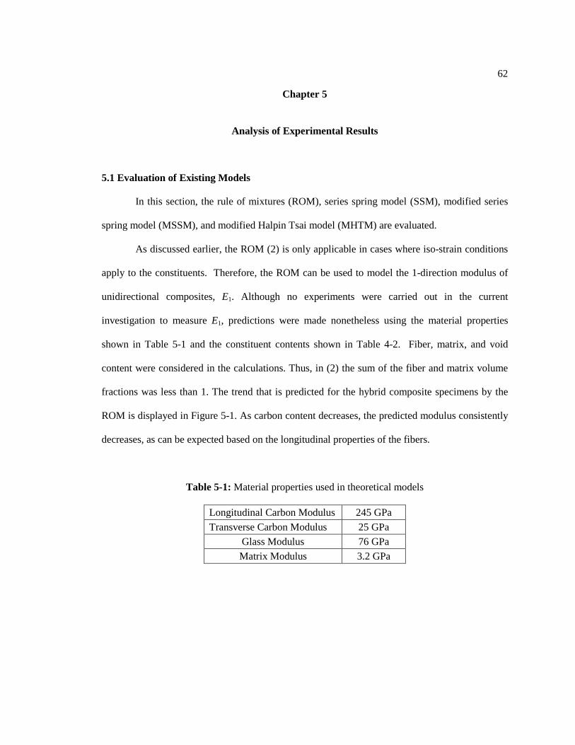
62

Chapter 5

Analysis of Experimental Results

5.1 Evaluation of Existing Models

In this section, the rule of mixtures (ROM), series spring model (SSM), modified series

spring model (MSSM), and modified Halpin Tsai model (MHTM) are evaluated.

As discussed earlier, the ROM (2) is only applicable in cases where iso-strain conditions

apply to the constituents. Therefore, the ROM can be used to model the 1-direction modulus of

unidirectional composites, E1. Although no experiments were carried out in the current

investigation to measure E1, predictions were made nonetheless using the material properties

shown in Table 5-1 and the constituent contents shown in Table 4-2. Fiber, matrix, and void

content were considered in the calculations. Thus, in (2) the sum of the fiber and matrix volume

fractions was less than 1. The trend that is predicted for the hybrid composite specimens by the

ROM is displayed in Figure 5-1. As carbon content decreases, the predicted modulus consistently

decreases, as can be expected based on the longitudinal properties of the fibers.

Table 5-1: Material properties used in theoretical models

Longitudinal Carbon Modulus 245 GPa Transverse Carbon Modulus 25 GPa

Glass Modulus 76 GPa Matrix Modulus 3.2 GPa

63

Figure 5-1: ROM for modulus of composite hybrids in the 1-direction

For the transverse modulus, the experimental data were compared to the SSM, MSSM,

and MHTM. The correlation between experimental data and models was measured with the

coefficient of determination (Wikipedia, 2013), R2 given by (40-43),

𝑦 =1𝑛𝑦𝑖

𝑛

𝑖=1

(40)

𝑆𝑆𝑟𝑒𝑠 = (𝑦𝑖 − 𝑓𝑖)2𝑛

𝑖=1

(41)

𝑆𝑆𝑡𝑜𝑡 = (𝑦𝑖 − 𝑦)2𝑛

𝑖=1

(42)

𝑅2 ≡ 1 −𝑆𝑆𝑟𝑒𝑠𝑆𝑆𝑡𝑜𝑡

(43)

where,

0

20

40

60

80

100

120

140

160

180

0 25 50 75 100

E 1 (G

Pa)

Glass Fiber Volume (%) of Reinforcement Content

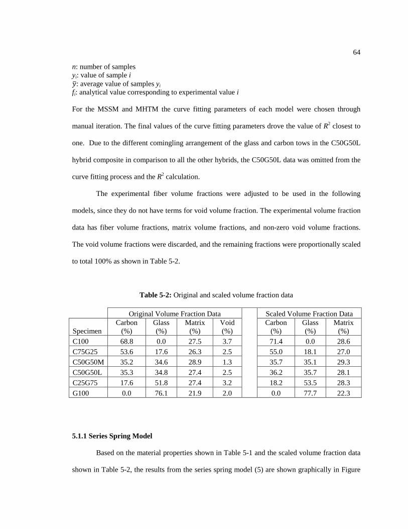
64

n: number of samples yi: value of sample i 𝑦: average value of samples yi fi: analytical value corresponding to experimental value i

For the MSSM and MHTM the curve fitting parameters of each model were chosen through

manual iteration. The final values of the curve fitting parameters drove the value of R2 closest to

one. Due to the different comingling arrangement of the glass and carbon tows in the C50G50L

hybrid composite in comparison to all the other hybrids, the C50G50L data was omitted from the

curve fitting process and the R2 calculation.

The experimental fiber volume fractions were adjusted to be used in the following

models, since they do not have terms for void volume fraction. The experimental volume fraction

data has fiber volume fractions, matrix volume fractions, and non-zero void volume fractions.

The void volume fractions were discarded, and the remaining fractions were proportionally scaled

to total 100% as shown in Table 5-2.

Table 5-2: Original and scaled volume fraction data

Original Volume Fraction Data Scaled Volume Fraction Data

Specimen Carbon

(%) Glass (%)

Matrix (%)

Void (%)

Carbon (%)

Glass (%)

Matrix (%)

C100 68.8 0.0 27.5 3.7 71.4 0.0 28.6 C75G25 53.6 17.6 26.3 2.5 55.0 18.1 27.0 C50G50M 35.2 34.6 28.9 1.3 35.7 35.1 29.3 C50G50L 35.3 34.8 27.4 2.5 36.2 35.7 28.1 C25G75 17.6 51.8 27.4 3.2 18.2 53.5 28.3 G100 0.0 76.1 21.9 2.0 0.0 77.7 22.3

5.1.1 Series Spring Model

Based on the material properties shown in Table 5-1 and the scaled volume fraction data

shown in Table 5-2, the results from the series spring model (5) are shown graphically in Figure

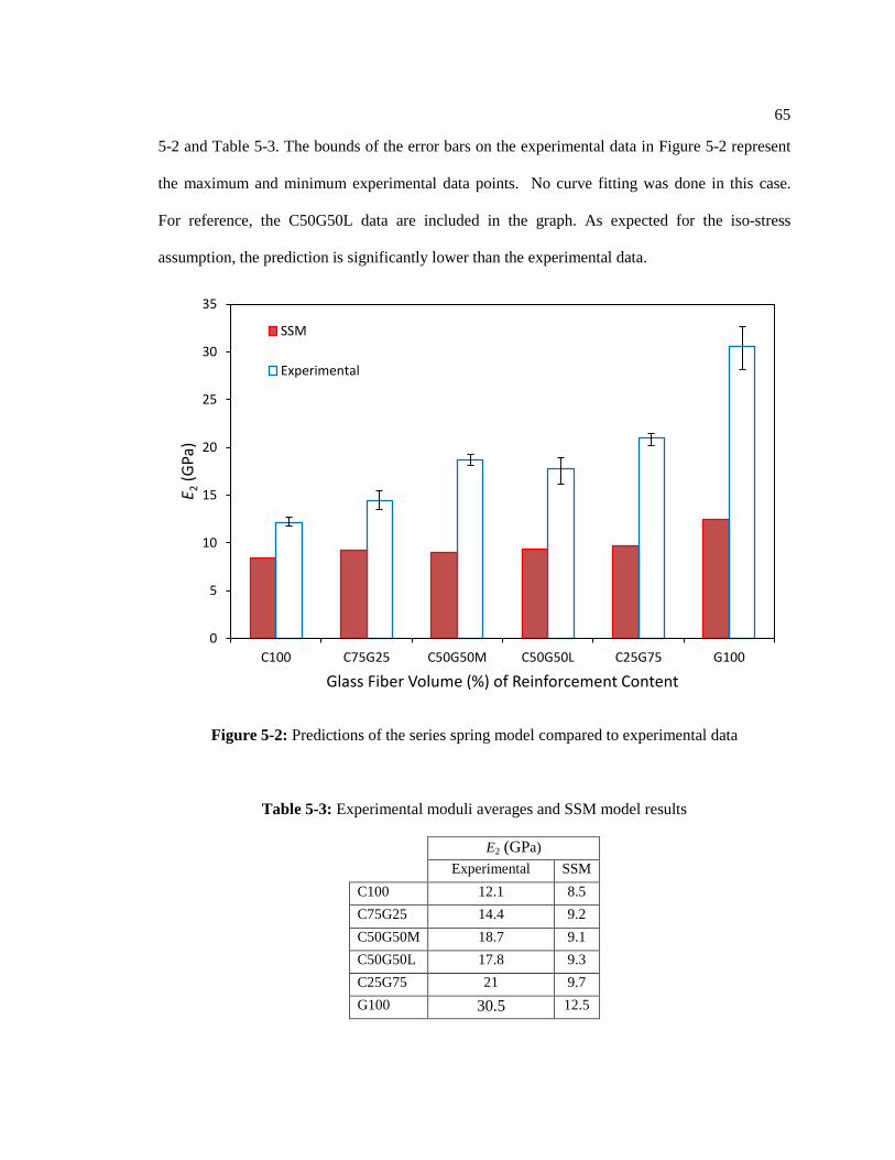
65

5-2 and Table 5-3. The bounds of the error bars on the experimental data in Figure 5-2 represent

the maximum and minimum experimental data points. No curve fitting was done in this case.

For reference, the C50G50L data are included in the graph. As expected for the iso-stress

assumption, the prediction is significantly lower than the experimental data.

Figure 5-2: Predictions of the series spring model compared to experimental data

Table 5-3: Experimental moduli averages and SSM model results

E2 (GPa) Experimental SSM C100 12.1 8.5 C75G25 14.4 9.2 C50G50M 18.7 9.1 C50G50L 17.8 9.3 C25G75 21 9.7 G100 30.5 12.5

0

5

10

15

20

25

30

35

C100 C75G25 C50G50M C50G50L C25G75 G100

E 2 (G

Pa)

Glass Fiber Volume (%) of Reinforcement Content

SSM

Experimental

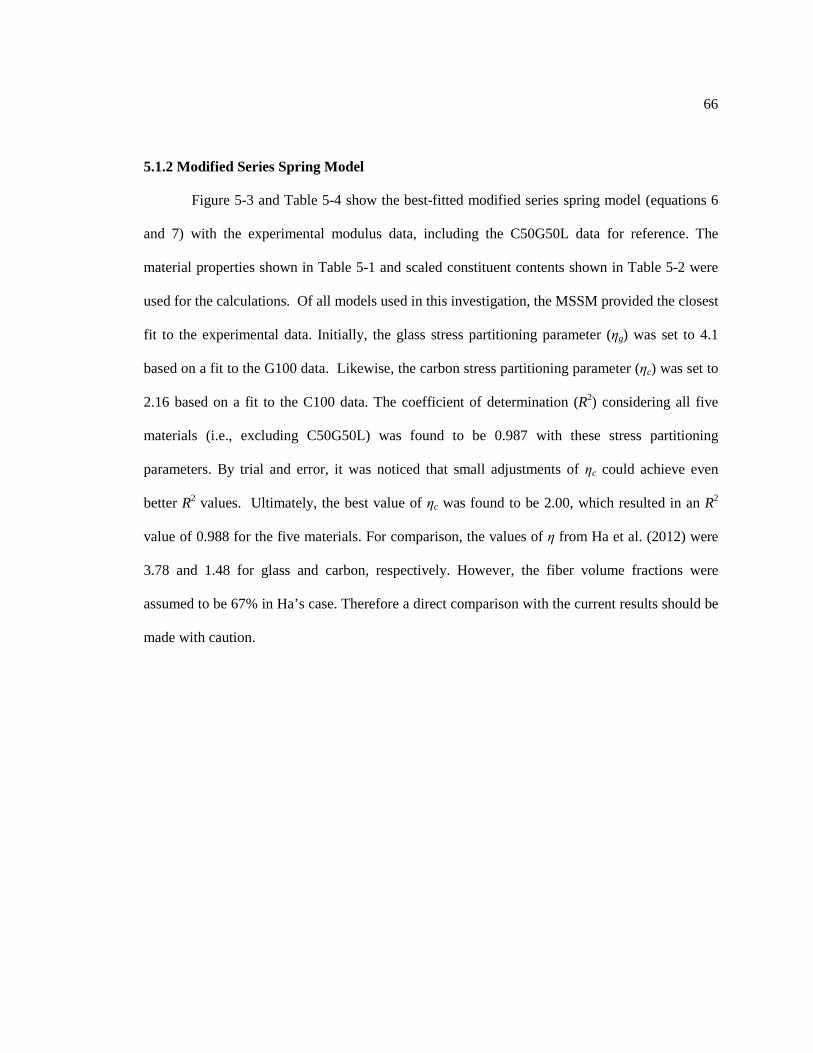
66

5.1.2 Modified Series Spring Model

Figure 5-3 and Table 5-4 show the best-fitted modified series spring model (equations 6

and 7) with the experimental modulus data, including the C50G50L data for reference. The

material properties shown in Table 5-1 and scaled constituent contents shown in Table 5-2 were

used for the calculations. Of all models used in this investigation, the MSSM provided the closest

fit to the experimental data. Initially, the glass stress partitioning parameter (ηg) was set to 4.1

based on a fit to the G100 data. Likewise, the carbon stress partitioning parameter (ηc) was set to

2.16 based on a fit to the C100 data. The coefficient of determination (R2) considering all five

materials (i.e., excluding C50G50L) was found to be 0.987 with these stress partitioning

parameters. By trial and error, it was noticed that small adjustments of ηc could achieve even

better R2 values. Ultimately, the best value of ηc was found to be 2.00, which resulted in an R2

value of 0.988 for the five materials. For comparison, the values of η from Ha et al. (2012) were

3.78 and 1.48 for glass and carbon, respectively. However, the fiber volume fractions were

assumed to be 67% in Ha’s case. Therefore a direct comparison with the current results should be

made with caution.

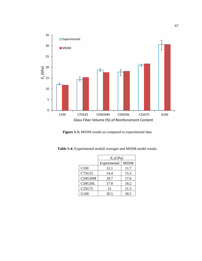
67

Figure 5-3: MSSM results as compared to experimental data

Table 5-4: Experimental moduli averages and MSSM model results

E2 (GPa)

Experimental MSSM

C100 12.1 11.7 C75G25 14.4 15.3 C50G50M 18.7 17.6 C50G50L 17.8 18.2 C25G75 21 21.5 G100 30.5 30.5

0

5

10

15

20

25

30

35

C100 C75G25 C50G50M C50G50L C25G75 G100

E 2 (G

Pa)

Glass Fiber Volume (%) of Reinforcement Content

Experimental

MSSM

68

5.1.3 Modified Halpin Tsai

The best-fitted MHTM (10), (11), (12) resulted in the comparison shown in Figure 5-4

and Table 5-5. Once again, the C50G50L hybrid is shown only for reference, as it was not used

in the model fitting procedure. Also, material properties were taken from Table 5-1 and the

scaled constituent contents from Table 5-2. The model was outside of the experimental scatter for

three cases. The R2 for these results is 0.952, and the best-fit value of ξ is 3.45. The correlation

was significantly better than the SSM, but worse than the MSSM. The value of ξ typically lies

within 1 and 2 for the unmodified Halpin Tsai model, as mentioned in the literature review.

Figure 5-4: MHTM results as compared to experimental data

0

5

10

15

20

25

30

35

C100 C75G25 C50G50M C50G50L C25G75 G100

E 2 (G

Pa)

Glass Fiber Volume (%) of Reinforcement Content

Experimental

MHTM

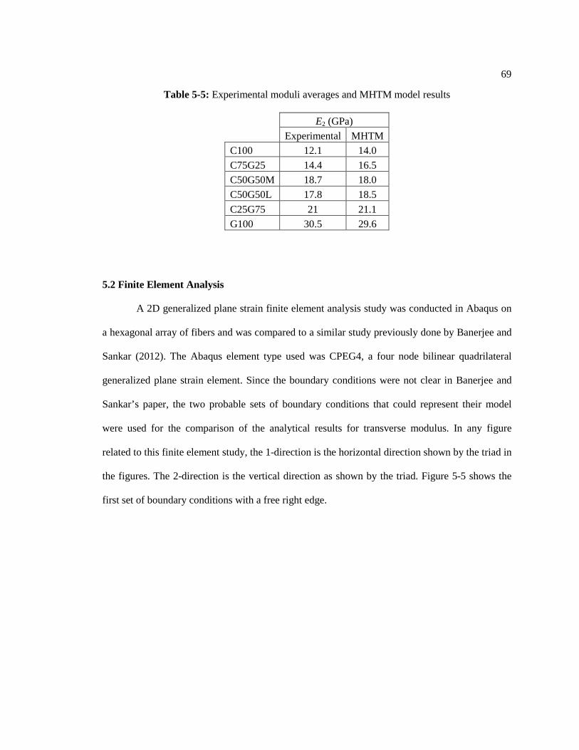
69

Table 5-5: Experimental moduli averages and MHTM model results

E2 (GPa)

Experimental MHTM

C100 12.1 14.0 C75G25 14.4 16.5 C50G50M 18.7 18.0 C50G50L 17.8 18.5 C25G75 21 21.1 G100 30.5 29.6

5.2 Finite Element Analysis

A 2D generalized plane strain finite element analysis study was conducted in Abaqus on

a hexagonal array of fibers and was compared to a similar study previously done by Banerjee and

Sankar (2012). The Abaqus element type used was CPEG4, a four node bilinear quadrilateral

generalized plane strain element. Since the boundary conditions were not clear in Banerjee and

Sankar’s paper, the two probable sets of boundary conditions that could represent their model

were used for the comparison of the analytical results for transverse modulus. In any figure

related to this finite element study, the 1-direction is the horizontal direction shown by the triad in

the figures. The 2-direction is the vertical direction as shown by the triad. Figure 5-5 shows the

first set of boundary conditions with a free right edge.

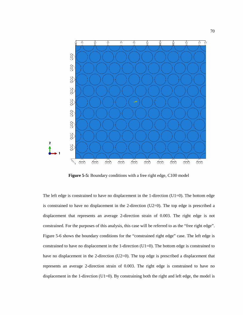
70

Figure 5-5: Boundary conditions with a free right edge, C100 model

The left edge is constrained to have no displacement in the 1-direction (U1=0). The bottom edge

is constrained to have no displacement in the 2-direction (U2=0). The top edge is prescribed a

displacement that represents an average 2-direction strain of 0.003. The right edge is not

constrained. For the purposes of this analysis, this case will be referred to as the “free right edge”.

Figure 5-6 shows the boundary conditions for the “constrained right edge” case. The left edge is

constrained to have no displacement in the 1-direction (U1=0). The bottom edge is constrained to

have no displacement in the 2-direction (U2=0). The top edge is prescribed a displacement that

represents an average 2-direction strain of 0.003. The right edge is constrained to have no

displacement in the 1-direction (U1=0). By constraining both the right and left edge, the model is

71

not permitted to displace in the 1-direction. This causes the model to appear stiffer than the free

right edge case when calculating the modulus.

Figure 5-6: Boundary conditions with a constrained right edge, G100 model

A sensitivity analysis was conducted based on model mesh size and the calculated

transverse modulus from each study. The modulus was calculated from the model output as

shown in equation (44).

𝐸2 =

1𝜀2𝐹𝑡𝑜𝑡𝑎𝑙𝐴𝑡𝑜𝑡𝑎𝑙

(44)

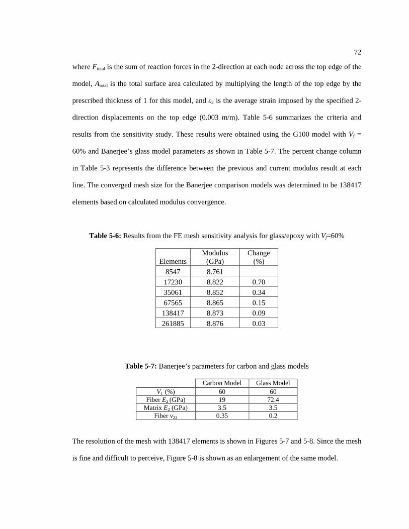
72

where Ftotal is the sum of reaction forces in the 2-direction at each node across the top edge of the

model, Atotal is the total surface area calculated by multiplying the length of the top edge by the

prescribed thickness of 1 for this model, and ε2 is the average strain imposed by the specified 2-

direction displacements on the top edge (0.003 m/m). Table 5-6 summarizes the criteria and

results from the sensitivity study. These results were obtained using the G100 model with Vf =

60% and Banerjee’s glass model parameters as shown in Table 5-7. The percent change column

in Table 5-3 represents the difference between the previous and current modulus result at each

line. The converged mesh size for the Banerjee comparison models was determined to be 138417

elements based on calculated modulus convergence.

Table 5-6: Results from the FE mesh sensitivity analysis for glass/epoxy with Vf=60%

Elements Modulus

(GPa) Change

(%) 8547 8.761

17230 8.822 0.70 35061 8.852 0.34 67565 8.865 0.15 138417 8.873 0.09 261885 8.876 0.03

Table 5-7: Banerjee’s parameters for carbon and glass models

Carbon Model Glass Model Vf (%) 60 60

Fiber E2 (GPa) 19 72.4 Matrix E2 (GPa) 3.5 3.5

Fiber v23 0.35 0.2

The resolution of the mesh with 138417 elements is shown in Figures 5-7 and 5-8. Since the mesh

is fine and difficult to perceive, Figure 5-8 is shown as an enlargement of the same model.

73

Figure 5-7: Full view of the G100 model with 138417 elements

Figure 5-8: A selected section of the G100 model with 138417 elements

fiber boundary

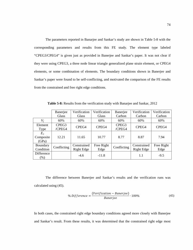
74

The parameters reported in Banarjee and Sankar’s study are shown in Table 5-8 with the

corresponding parameters and results from this FE study. The element type labeled

“CPEG3/CPEG4” is given just as provided in Banerjee and Sankar’s paper. It was not clear if

they were using CPEG3, a three node linear triangle generalized plane strain element, or CPEG4

elements, or some combination of elements. The boundary conditions shown in Banerjee and

Sankar’s paper were found to be self-conflicting, and motivated the comparison of the FE results

from the constrained and free right edge conditions.

Table 5-8: Results from the verification study with Banarjee and Sankar, 2012

The difference between Banerjee and Sankar’s results and the verification runs was

calculated using (45).

% 𝐷𝑖𝑓𝑓𝑒𝑟𝑒𝑛𝑐𝑒 =

(𝑉𝑒𝑟𝑖𝑓𝑖𝑐𝑎𝑡𝑖𝑜𝑛 − 𝐵𝑎𝑛𝑒𝑟𝑗𝑒𝑒)𝐵𝑎𝑛𝑒𝑟𝑗𝑒𝑒

∙ 100% (45)

In both cases, the constrained right edge boundary conditions agreed more closely with Banerjee

and Sankar’s result. From these results, it was determined that the constrained right edge most

Banerjee Glass

Verification Glass

Verification Glass

Banerjee Carbon

Verification Carbon

Verification Carbon

Vf 60% 60% 60% 60% 60% 60% Element

Type CPEG3 /CPEG4 CPEG4 CPEG4 CPEG3

/CPEG4 CPEG4 CPEG4

E2 Composite

(GPa) 12.21 11.65 10.77 8.77 8.87 7.94

Boundary Condition Conflicting Constrained

Right Edge Free Right

Edge Conflicting Constrained Right Edge

Free Right Edge

Difference (%) -4.6 -11.8 1.1 -9.5

75

closely agreed with the results from Banerjee and Sankar’s paper. However, it is known that

constraining both lateral edges causes the modulus according to (44) to be too high. Based on this

consideration, the free right edge condition was chosen for the FE studies conducted and

compared to the current experimental specimen results.

Two FE studies were done to evaluate the experimental results. The parameters for each

model are listed in Table 5-9. The stress field in the 2-direction for the G100 model is shown in

Figure 5-9. The mesh in Figure 5-9 is too fine to see at the scale shown, so Figure 5-10 is

provided which shows a small portion of the same mesh which was used to evaluate stress

partitioning parameters (η = σf/σm). The portion shown in Figure 5-10 is highlighted by a

rectangle in Figure 5-9.

Table 5-9: Parameters used in FE studies for comparison to experimental results

C100 Model

G100 Model

Element Type CPEG4 CPEG4 Elements 105411 143553 Specimen Vr (%) 68.8 76.1 FEA Vr (%) 68.3 76.2 Fiber E2 (GPa) 24.82 76 Matrix E (GPa) 3.2 3.2 Fiber νT 0.005 0.2 Matrix νT 0.35* 0.35* Strain ε 0.003 0.003

*value from Banerjee and Sankar (2012)

76

Figure 5-9: Stress field showing stress components in the 2-direction (Y-direction) for the G100

model, rectangle over portion of model shown in Figure 5-10

77

Figure 5-10: Symmetric portion of the G100 model used to compute stress partitioning

parameters based on stress in the direction of loading (2- or Y-direction)

The following parameters were calculated from the results of each study: the transverse

elastic modulus of the composite, the stress partitioning parameter based on stress in the 2-

direction (η = σf/σm), and the overall average stress in the 2-direction. The stress partitioning

parameter was computed by taking the average stress in the 2-direction from all of the integration

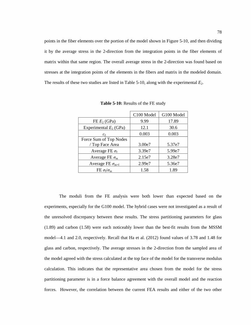
78

points in the fiber elements over the portion of the model shown in Figure 5-10, and then dividing

it by the average stress in the 2-direction from the integration points in the fiber elements of

matrix within that same region. The overall average stress in the 2-direction was found based on

stresses at the integration points of the elements in the fibers and matrix in the modeled domain.

The results of these two studies are listed in Table 5-10, along with the experimental E2.

Table 5-10: Results of the FE study

C100 Model G100 Model

FE E2 (GPa) 9.99 17.89 Experimental E2 (GPa) 12.1 30.6

ε2 0.003 0.003 Force Sum of Top Nodes

/ Top Face Area 3.00e7 5.37e7 Average FE σf 3.39e7 5.99e7 Average FE σm 2.15e7 3.28e7

Average FE σm+f 2.99e7 5.36e7 FE σf/σm 1.58 1.89

The moduli from the FE analysis were both lower than expected based on the

experiments, especially for the G100 model. The hybrid cases were not investigated as a result of

the unresolved discrepancy between these results. The stress partitioning parameters for glass

(1.89) and carbon (1.58) were each noticeably lower than the best-fit results from the MSSM

model—4.1 and 2.0, respectively. Recall that Ha et al. (2012) found values of 3.78 and 1.48 for

glass and carbon, respectively. The average stresses in the 2-direction from the sampled area of

the model agreed with the stress calculated at the top face of the model for the transverse modulus

calculation. This indicates that the representative area chosen from the model for the stress

partitioning parameter is in a force balance agreement with the overall model and the reaction

forces. However, the correlation between the current FEA results and either of the two other

79

results in the literature was not close at all. Further investigation is needed to resolve these

discrepancies.

5.3 Summary of Models

The MSSM and the MHTM semi-empirical models were able to be calibrated well to the

experimental transverse modulus data by adjusting their curve fitting parameters. It was not

uncommon to find the MSSM or MHTM model “predictions” within the scatter of the

experimental data. Mathematically, the MSSM had the best correlation with a R2 value of 0.988,

followed by the MHTM with a R2 value of 0.952. These results are summarized graphically in

Figure 5-11, where the error bars on the experimental data bars represent the maxima and minima

of the experimental set. The SSM and the FE analysis were both low in terms of modulus, and did

not show agreement with even the non-hybrid composites.

An inspection of the microstructure of the C50G50L sample lends to the possible use of

the ROM for a prediction of material properties. The ROM (2) is based on the isostrain principle,

and since the glass/epoxy and carbon/epoxy regions in this specimen appeared in layers, the

isostrain principle could appropriate for modeling the behavior of this specimen. A version of the

ROM equation (2) in the form of (46) was used to calculate a transverse modulus based on the

glass/epoxy and carbon/epoxy layer properties in Table 4-5:

𝐸2𝑠 = 𝑉𝑐/𝑒𝐸2𝑐/𝑒 + 𝑉𝑔/𝑒𝐸2𝑐/𝑒 (46)

where,

E2s: transverse elastic modulus of composite Vc/e: volume fraction of carbon epoxy composite Vg/e: volume fraction of glass epoxy composite E2c/e: transverse modulus of carbon epoxy composite E2g/e: transverse modulus of glass composite

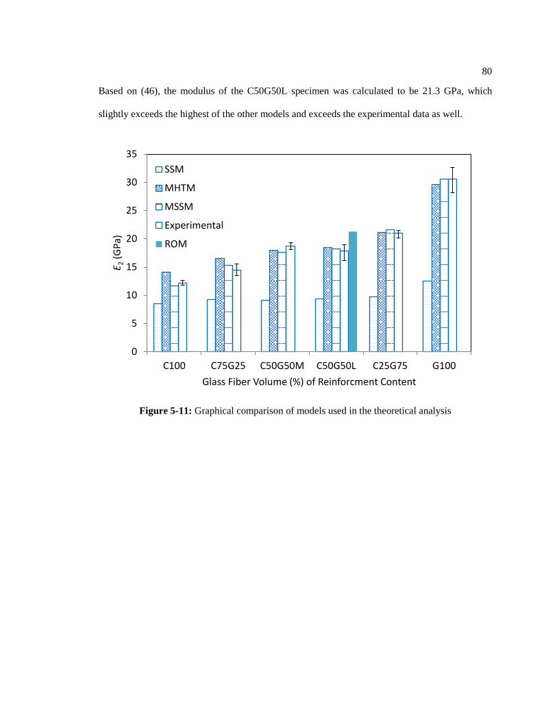
80

Based on (46), the modulus of the C50G50L specimen was calculated to be 21.3 GPa, which

slightly exceeds the highest of the other models and exceeds the experimental data as well.

Figure 5-11: Graphical comparison of models used in the theoretical analysis

0

5

10

15

20

25

30

35

C100 C75G25 C50G50M C50G50L C25G75 G100

E 2 (G

Pa)

Glass Fiber Volume (%) of Reinforcment Content

SSM

MHTM

MSSM

Experimental

ROM

81

Chapter 6

Conclusions and Recommendations

6.1 Conclusions

Previous investigations have provided extensive experimental and analytical information

on unidirectionally reinforced hybrid fiber composites. However, for the transverse direction,

only analytical models have been found. No experimental data are available, to-date. In addition,

little data is available for the transverse properties of carbon fibers, which are known to be

anisotropic. The lack of modulus and strength data for the transverse direction of hybrid

composites was the motivation for the current experimental investigation of commingled E-

glass/carbon/epoxy composites.

In this investigation, the transverse modulus of elasticity and tension-controlled flexural

strength of hybrid composites with commingled E-glass and carbon fibers were experimentally

evaluated using flexural tests. Six types of composite rings were hoop wound on a filament

winder, four of which were hybrid varieties. The strength and elastic modulus were found to

monotonically increase with increasing glass fiber content. For two different geometric

arrangements of comingled glass and fiber tows in a 50/50 proportion, little difference was seen

in the modulus or strength. The experimental modulus data were able to be modeled well with the

modified series spring model and the modified Halpin-Tsai model. Poor correlation was found

with the series spring model, which was not unexpected since this model is considered a lower-

bound. Although the FE results agreed within 1.1-4.6% with independently produced results in

the literature, they did not agree well with the experimental data measured in this investigation.

The FE results exhibited 17-42% lower transverse modulus than was experimentally determined,

and the FE analysis was therefore not applied to the hybrid composite cases.

82

The experimental modulus results appeared to be suspiciously high. Therefore, a several

checks on the experimental apparatus and procedure were done. These results suggest that the

load cell signal may be of the order of 5% high, and the beam geometry is suitable for use with

Euler-Bernoulli beam theory. The only factor that was not investigated thoroughly was the effect

of the bonded v-notched tabs on the measured strain.

6.2 Recommendations for Future Work

Future work should be conducted in this area of study to diversify the limited amount of

results available in the literature. The first category of experiments to be conducted is fiber type.

Different types of fibers should be used in a similar study, starting with other commonly used

fibers with significantly different properties, such as high modulus carbon fibers, S-Glass fibers,

and even other fiber types such as aramids. Within these experiments of fiber type, the fiber

content should be varied with higher resolution than in this study. In this study only three fiber

content hybridizations were studied, C25G75, C50G50, and C75G25. Ideally, twice this

resolution would be collected with six evenly spaced hybrids. Once the extremities, and ideally,

entire spectrum of fiber types have been tested, the next category of experiments that should be

explored is overall reinforcement content. The previous studies of specific fiber types should be

expanded upon, by repeating the same combinations of fiber types and hybridization fractions,

but with varying overall reinforcement content relative to matrix content. Tensile and

compression tests perpendicular to the fibers could be conducted to supplement the flexural data

obtained in the present investigation. A wider mandrel could be used in future winds so that

longer specimens may be extracted. In the present investigation, the beam lengths were limited to

the width of the mandrel (~75 mm), which limited the selection of available test methods.

Strain should be measured with strain gages rather than an extensometer with knife edges

resting in bonded metal tabs. The effect of the tabs on the measured strains was thought to be

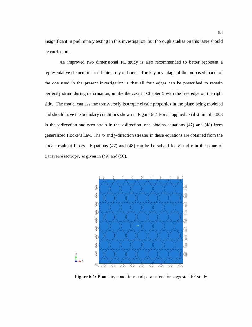
83

insignificant in preliminary testing in this investigation, but thorough studies on this issue should

be carried out.

An improved two dimensional FE study is also recommended to better represent a

representative element in an infinite array of fibers. The key advantage of the proposed model of

the one used in the present investigation is that all four edges can be prescribed to remain

perfectly strain during deformation, unlike the case in Chapter 5 with the free edge on the right

side. The model can assume transversely isotropic elastic properties in the plane being modeled

and should have the boundary conditions shown in Figure 6-2. For an applied axial strain of 0.003

in the y-direction and zero strain in the x-direction, one obtains equations (47) and (48) from

generalized Hooke’s Law. The x- and y-direction stresses in these equations are obtained from the

nodal resultant forces. Equations (47) and (48) can be be solved for E and v in the plane of

transverse isotropy, as given in (49) and (50).

Figure 6-1: Boundary conditions and parameters for suggested FE study

84

𝜀𝑥 = 0 = 𝜎𝑥𝐸−𝜎𝑦𝑣𝐸

(47)

𝜀𝑦 = 0.003 = 𝜎𝑦𝐸−𝜎𝑥𝑣𝐸

(48)

𝑣 =

𝜎𝑥𝜎𝑦

(49)

𝐸 =

𝜎𝑦 −𝜎𝑥2𝜎𝑦

0.003

(50)

85

References

Altenbach, H., Altenbach, J., and Kissing, W., 2004. Mechanics of Composite Structural

Elements. New York: Springer-Verlag.

ASTM International. 2013. D5229/D5229M – 12 Standard Test Method for Moisture Absorption

Properties and Equilibrium Conditioning of Polymer Matrix Composite Materials. West

Conshohocken, PA.

ASTM International. 2013. D6272 – 10 Standard Test Method for Flexural Properties of

Unreinforced and Reinforced Plastics and Electrical Insulating Matrials by Four-Point Bending.

West Conshohocken, PA.

Bakis, C., Nanni, A., Terosky, J., and Koehler, S., 2001, “Self-monitoring, Pseudo-ductile,

Hybrid FRP Reinforcement Rods for Concrete Applications,” Composites Science and

Technology, 61:815-823

Banerjee, S., and Sankar, B., “Mechanical Properties of Hybrid Composites Using Finite Element

Method Based Micromechanics,” Proc. 27th Annual Technical Conference of the American

Society for Composites, DEStech, Lancaster, Pa., 2012 (CD ROM).

Bunsell, A., and Harris, B., 1974. “Hybrid Carbon and Glass Fibre Composites,” Composites,

5(4):157-164.

86

Deng, A., Ye, L., and Mai, Y., 1999. “Influence of Fibre Cross-sectional Aspect Ratio on

Mechanical Properties of Glass Fibre/Epoxy Composites I. Tensile and Flexure Behaviour.”

Composites Science and Technology. 59:1331-1339

Daniel, I., and Ishai, O. 2006. Engineering Mechanics of Composite Materials. New York:

Oxford University Press.

Fu, S., Hu, X., and Yue, C., 1998. “A New Model for the Transverse Modulus of Unidirectional

Fiber Composites,” Journal of Materials Science, 33:4953-4960.

Gabrys, C., 1996. “Design, Fabrication and Testing of Advanced Composite Energy Storage

Flywheels.” Ph.D. Dissertation. The Pennsylvania State University, University Park, PA.

Genta, G. 1985. Kinetic Energy Storage. London: Butterworth & Co. Ltd.

Ha, S., Yang, H., and Kim, D., 1999. “Optimal Design of a Hybrid Composite Flywheel with a

Permanent Magnet Rotor,” Journal of Composite Materials, 33(16):1544–1575.

Ha, S., Kim, S., Nasir, S., and Han, S., 2012. “Design Optimization and Fabrication of a Hybrid

Composite Flywheel Rotor,” Composite Structures, 94:3290-3299.

Halpin, J., and Kardos, J., 1976. “The Halpin-Tsai Equations: A Review,” Polymer Engineering

and Science, 16(5):344-352.

87

Hamed, A., Hamdan, M., Sahari, B., and Sapuan, S., 2008. “Experimental Characterization of

Filament Wound Glass/Epoxy and Carbon/Epoxy Composite Materials,” ARPN Journal of

Engineering and Applied Sciences, 3(4):76-87.

Hayashi T., 1972. “On the Improvement of Mechanical Properties of Composites by Hybrid

Composition,” Proc. 8th International Reinforced Plastics Conference, paper 22. Brighton (UK):

British Plastics Federation, 149-52.

Henry, T., 2012. “Static and Dynamic Characterization of Composite Materials for Future

Driveshaft Systems.” Master of Science Thesis. The Pennsylvania State University.

Hexcel HexTow AS4D Data Sheet. 2013. Hexcel Corporation.

Huang, J., Qunhua, L., Yang, Q., Huijun, L., Wei, Y., 2012. “Measurement and Research of the

Transverse Mechanical Properties of High Performance Fibers.” Key Engineering Materials,

492:384-387.

Ko, Y.-F., Ju, J. W., 2013. “Effective Transverse Elastic Moduli of Three-Phase Hybrid Fiber-

Reinforced Composites with Randomly Located and Interacting Aligned Circular Fibers of

Distinct Elastic Properties and Sizes,” Acta Mechanica, 224:157-182.

Marom, G., Fischer, S., Tuler, F., and Wagner, H., 1978. “Hybrid Effects in Composites:

Conditions for Positive or Negative Effects Versus Rule-of-Mixtures Behaviour,” Journal of

Materials Science, 13:1419-1426.

88

Miyagawa, H., Sato, C., Mase, T., Drown, E., Drzal, L., and Ikegami, K., 2005. “Transverse

Elastic Modulus of Carbon Fibers Measured by Raman Spectroscopy,” Materials Science and

Engineering A, 412:88-92.

Momentive Technical Data Sheet EPON Resin 862. Momentive Specialty Chemicals Inc. HCD-

3950. Rev 6/5/2013.

Owens Corning Composite Solutions Reinforcement Guide. 2011. Owens Corning.

Phoenix, S., and Skelton, J., 1974. “Transverse Compressive Moduli and Yield Behavior of Some

Orthotropic, High-Modulus Filaments.” Textile Research Journal, 44:934-940

PPG Industries Fiber Glass Americas, 2013., Private communication with Bruce Parson of PPG

Industries Fiber Glass Americas. May 29.

PPG Technical Data Sheet Hybon 2022 Roving. 2013. PPG Fiber Glass.

PPG Fiber Glass HS2 & HS4 High Strength Fiber Glass Data Sheet. 2013. PPG Fiber Glass.

Ranganathan, S., and Mantena, P., 2003. “Axial Loading and Buckling Response Characteristics

of Pultruded Hybrid Glass-Graphite/Epoxy Composite Beams.” Journal of Reinforced Plastics

and Composites, 22(7):671-679

Sharma, A., and Bakis, C., 2006. “C-Shape Specimen for Tensile Radial Strength of Thick,

Filament-wound Rings.” Journal of Composite Materials, 40(2):97-117

89

Short, D., and Summerscales, J., 1980. “Hybrids – a Review.” Composites, 33-38

Strait, L., and Rude, T., 1998. “Measurement of Fiber Density by Helium Pycnometry,” Applied

Research Laboratory. Technical Memorandum.

Toray T1000G Technical Data Sheet. 2013. Toray Carbon Fibers America, Inc.

Tsai, S., and Hahn, H., 1980. Introduction to Composite Materials. CRC Press.

Wikipedia. 2013. “Coefficient of Determination,” June 27.

http://en.wikipedia.org/wiki/Coefficient_of_determination

Žmindák, M., Riecky, D., and Dudinský, M., 2011. “Finite Element Analysis of Viscoelastic

Composite Solids.” Modelling of Mechanical and Mechatronic Systems. The 4th International

Conference. 576-585

90

Appendix A

Electrical Setup of Mandrel Heater

The wiring schematic of the ring heaters on the mandrel is given in Figure A-1.

Figure A-1: Wiring schematic of ring heater circuit

The use of slip rings with the winder requires the proper positioning of the brushes as

shown in Figure A-2. The brushes are attached to a stool with a heavy iron cylinder and slid

inward until proper contact is achieved between the curvature of the brushes and slip rings. It is

important that the base for the brushes be weighted heavily; otherwise the motion of the slip rings

will cause the brush stand to topple over. In turn, the brushes will contact during the toppling

incident, cause a short circuit, blow the fuse in the knife switch box, and possibly cause other

damage.

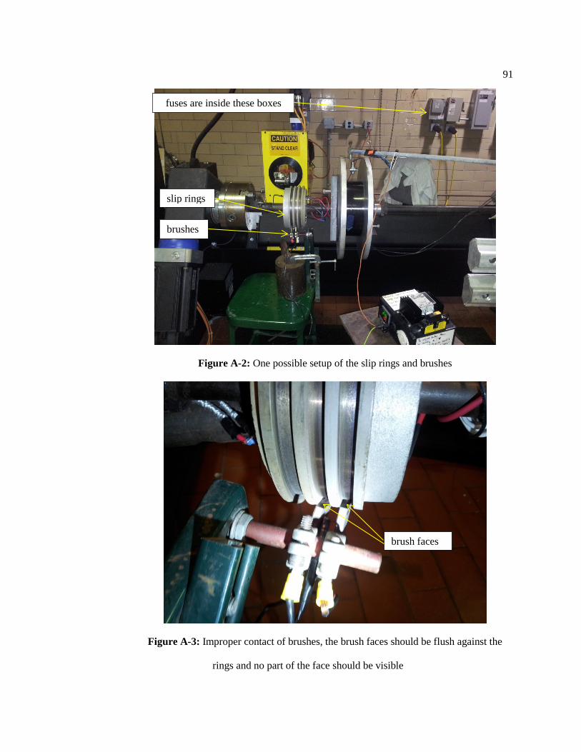
91

Figure A-2: One possible setup of the slip rings and brushes

Figure A-3: Improper contact of brushes, the brush faces should be flush against the

rings and no part of the face should be visible

slip rings

brushes

fuses are inside these boxes

brush faces

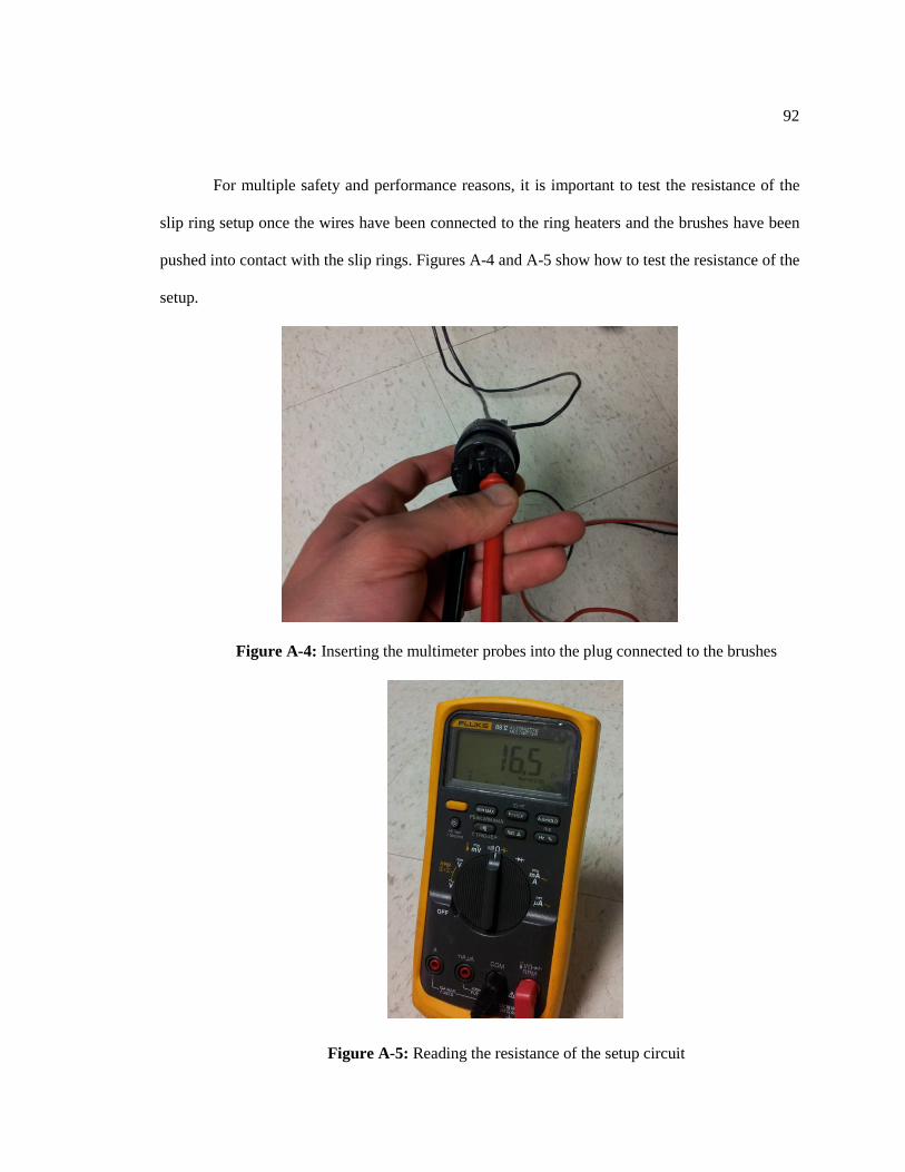
92

For multiple safety and performance reasons, it is important to test the resistance of the

slip ring setup once the wires have been connected to the ring heaters and the brushes have been

pushed into contact with the slip rings. Figures A-4 and A-5 show how to test the resistance of the

setup.

Figure A-4: Inserting the multimeter probes into the plug connected to the brushes

Figure A-5: Reading the resistance of the setup circuit

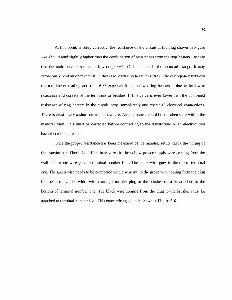
93

At this point, if setup correctly, the resistance of the circuit at the plug shown in Figure

A-4 should read slightly higher than the combination of resistances from the ring heaters. Be sure

that the multimeter is set to the low range ~600 Ω. If it is set in the automatic range, it may

erroneously read an open circuit. In this case, each ring heater was 8 Ω. The discrepancy between

the multimeter reading and the 16 Ω expected from the two ring heaters is due to lead wire

resistance and contact of the terminals or brushes. If this value is ever lower than the combined

resistance of ring heaters in the circuit, stop immediately and check all electrical connections.

There is most likely a short circuit somewhere. Another cause could be a broken wire within the

mandrel shaft. This must be corrected before connecting to the transformer or an electrocution

hazard could be present.

Once the proper resistance has been measured of the mandrel setup, check the wiring of

the transformer. There should be three wires in the yellow power supply wire coming from the

wall. The white wire goes to terminal number four. The black wire goes to the top of terminal

one. The green wire needs to be connected with a wire nut to the green wire coming from the plug

for the brushes. The white wire coming from the plug to the brushes must be attached to the

bottom of terminal number one. The black wire coming from the plug to the brushes must be

attached to terminal number five. This exact wiring setup is shown in Figure A-6.

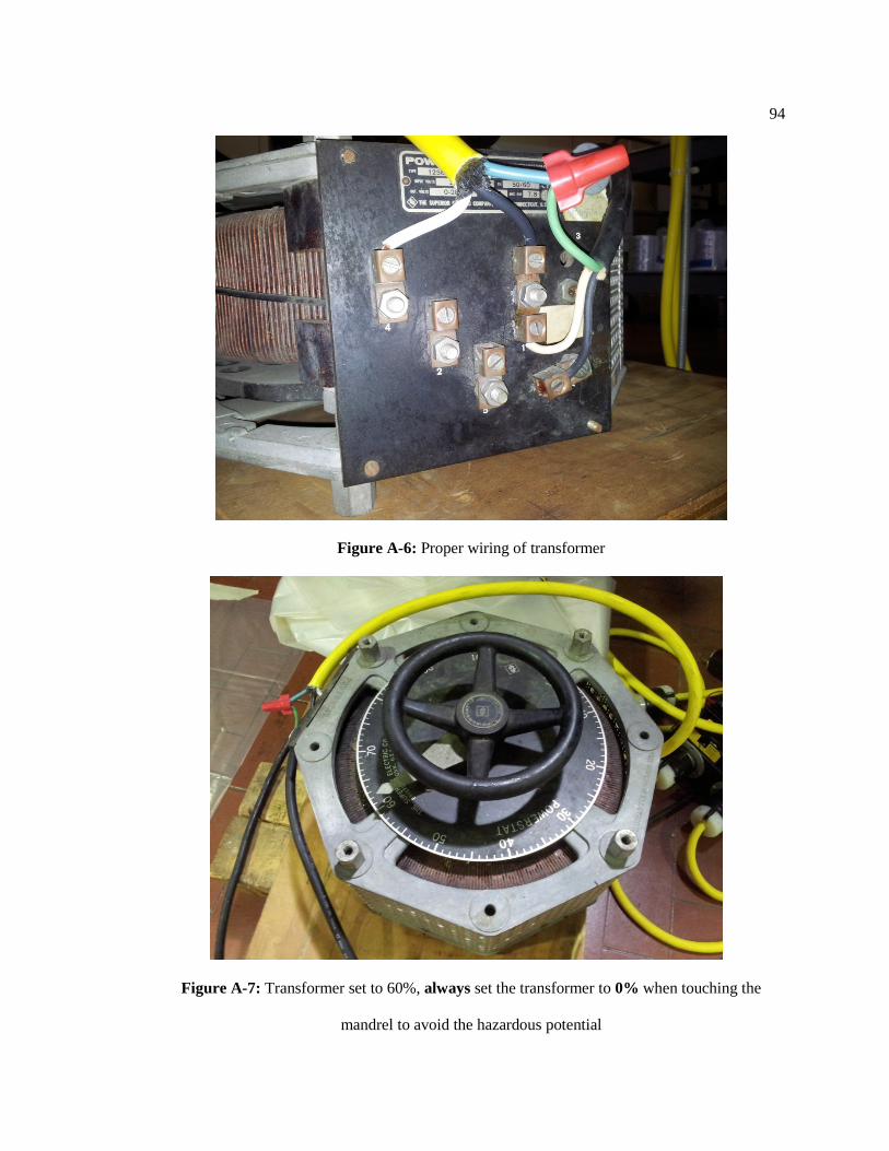
94

Figure A-6: Proper wiring of transformer

Figure A-7: Transformer set to 60%, always set the transformer to 0% when touching the

mandrel to avoid the hazardous potential

95

If the resistance of the mandrel tests correctly and the transformer wiring is verified, plug

the brushes into the output plug of the transformer. Once the wiring of the transformer and circuit

resistance has been checked, verify that the transformer is set to 0%. Finally, turn on the wall

power supply by engaging the knife edge boxes shown in Figure A-2.

96

Appendix B

Acid Digestion Setup and Safety Measures

Acid digestion is a process which can be very dangerous and result in serious injury if the

proper safety precautions are not in place. Before ever handling acid or working under the fume

hood, be sure to wear chemically resistant goggles, an approved chemical laboratory coat, and

gloves that are resistant to chemicals. Review all safety precautions before working with the acid,

and if the acid comes into contact with any personal safety equipment be sure to deal with it

appropriately before proceeding with the experiment.

In Figure B-1, the main vacuum line is attached to a splitter with two shutoff valves.

When filtering and washing the digested products, the acid and digested particles must be kept

separate from acetone and water. Vacuum is first pulled on the specimen using vacuum beaker #1

while it still contains acid. At this point only valve #1 is open. Once all of the acid has been

removed from the specimen in beaker #1, valve #1 should be closed. The filter may then be

transferred to vacuum beaker #2. Once the filter has been transferred to vacuum beaker #2, the

valve for vacuum beaker #2 may be opened. At this point the fibers should be washed with water,

and once with acetone as a final step to assist in drying.

• Never add acetone to acid

• Never add acid to acetone

• Never add water to acid

• Only add acid to water slowly if required

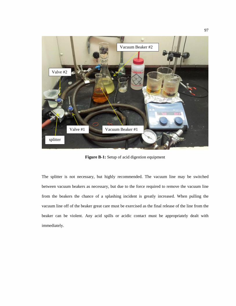
97

Figure B-1: Setup of acid digestion equipment

The splitter is not necessary, but highly recommended. The vacuum line may be switched

between vacuum beakers as necessary, but due to the force required to remove the vacuum line

from the beakers the chance of a splashing incident is greatly increased. When pulling the

vacuum line off of the beaker great care must be exercised as the final release of the line from the

beaker can be violent. Any acid spills or acidic contact must be appropriately dealt with

immediately.

Valve #1

Valve #2

Vacuum Beaker #1

Vacuum Beaker #2

splitter

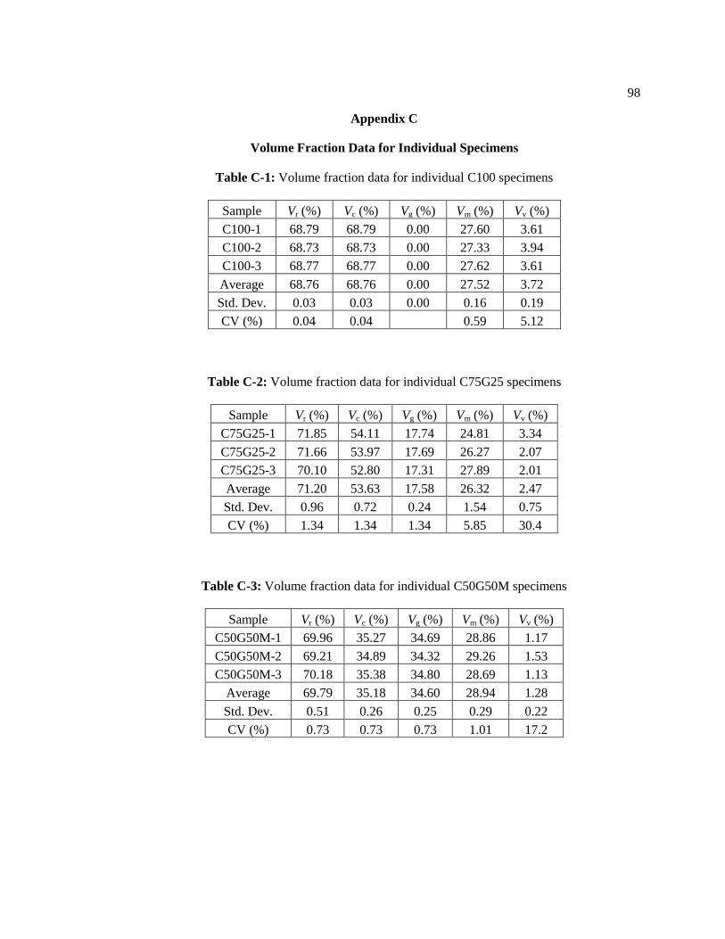
98

Appendix C

Volume Fraction Data for Individual Specimens

Table C-1: Volume fraction data for individual C100 specimens

Sample Vr (%) Vc (%) Vg (%) Vm (%) Vv (%) C100-1 68.79 68.79 0.00 27.60 3.61 C100-2 68.73 68.73 0.00 27.33 3.94 C100-3 68.77 68.77 0.00 27.62 3.61 Average 68.76 68.76 0.00 27.52 3.72 Std. Dev. 0.03 0.03 0.00 0.16 0.19 CV (%) 0.04 0.04

0.59 5.12

Table C-2: Volume fraction data for individual C75G25 specimens

Sample Vr (%) Vc (%) Vg (%) Vm (%) Vv (%) C75G25-1 71.85 54.11 17.74 24.81 3.34 C75G25-2 71.66 53.97 17.69 26.27 2.07 C75G25-3 70.10 52.80 17.31 27.89 2.01 Average 71.20 53.63 17.58 26.32 2.47 Std. Dev. 0.96 0.72 0.24 1.54 0.75 CV (%) 1.34 1.34 1.34 5.85 30.4

Table C-3: Volume fraction data for individual C50G50M specimens

Sample Vr (%) Vc (%) Vg (%) Vm (%) Vv (%) C50G50M-1 69.96 35.27 34.69 28.86 1.17 C50G50M-2 69.21 34.89 34.32 29.26 1.53 C50G50M-3 70.18 35.38 34.80 28.69 1.13

Average 69.79 35.18 34.60 28.94 1.28 Std. Dev. 0.51 0.26 0.25 0.29 0.22 CV (%) 0.73 0.73 0.73 1.01 17.2

99

Table C-4: Volume fraction data for individual C50G50L specimens

Sample Vr (%) Vc (%) Vg (%) Vm (%) Vv (%) C50G50L-1 70.20 35.39 34.81 27.82 1.97 C50G50L-2 69.98 35.28 34.70 27.48 2.55 C50G50L-3 70.12 35.35 34.77 26.86 3.02

Average 70.10 35.34 34.76 27.39 2.51 Std. Dev. 0.11 0.06 0.06 0.49 0.52 CV (%) 0.16 0.16 0.16 1.79 20.8

Table C-5: Volume fraction data for individual C25G75 specimens

Sample Vr (%) Vc (%) Vg (%) Vm (%) Vv (%) C25G75-1 69.03 17.48 51.56 28.12 2.85 C25G75-2 69.67 17.64 52.03 27.53 2.80 C25G75-3 69.43 17.57 51.85 26.48 4.09 Average 69.38 17.56 51.82 27.37 3.25 Std. Dev. 0.32 0.08 0.24 0.83 0.73 CV (%) 0.46 0.46 0.46 3.02 22.5

Table C-6: Volume fraction data for individual G100 specimens

Sample Vr (%) Vc (%) Vg (%) Vm (%) Vv (%) G100-1 76.21 0.00 76.21 21.69 2.10 G100-2 76.11 0.00 76.11 21.93 1.96 G100-3 76.09 0.00 76.09 21.97 1.95 Average 76.13 0.00 76.13 21.86 2.00 Std. Dev. 0.07 0.00 0.07 0.15 0.08 CV (%) 0.09 0.09 0.68 4.05

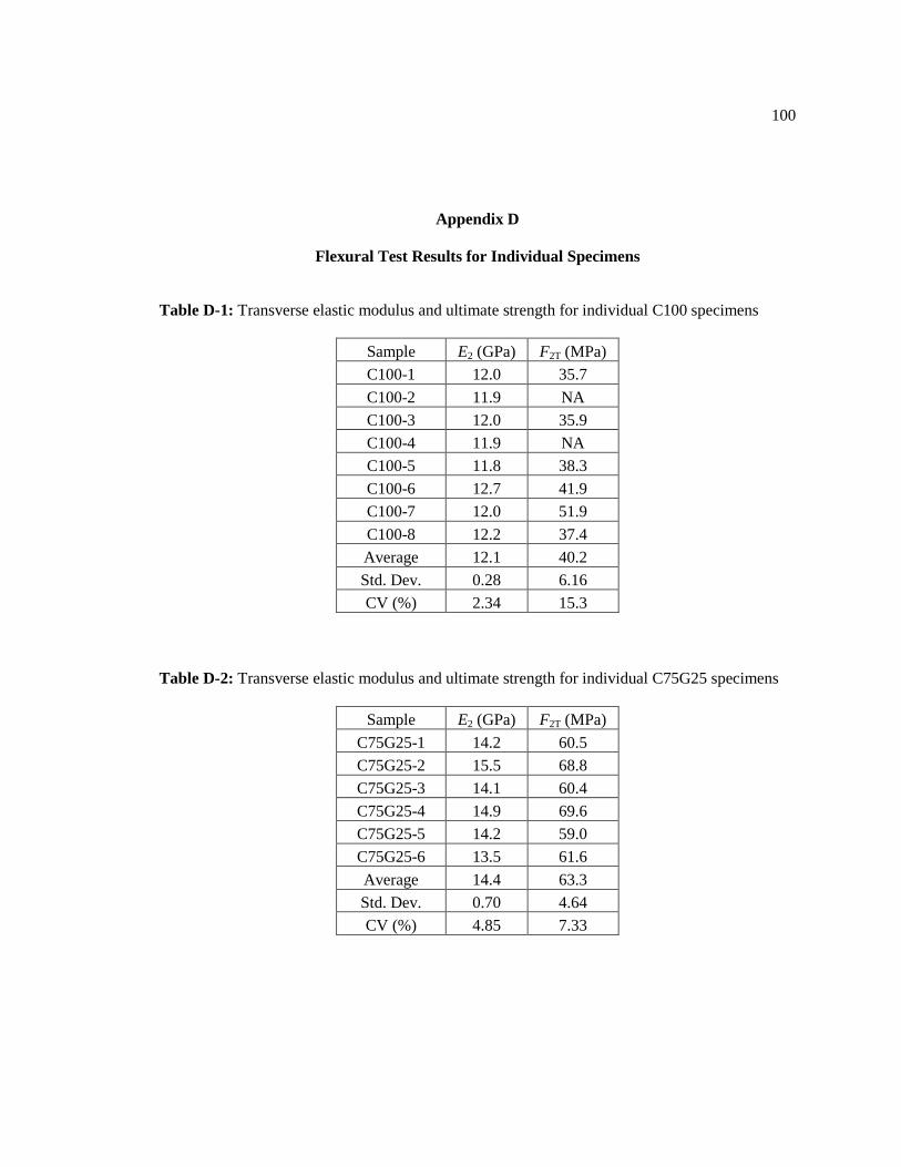
100

Appendix D

Flexural Test Results for Individual Specimens

Table D-1: Transverse elastic modulus and ultimate strength for individual C100 specimens

Sample E2 (GPa) F2T (MPa) C100-1 12.0 35.7 C100-2 11.9 NA C100-3 12.0 35.9 C100-4 11.9 NA C100-5 11.8 38.3 C100-6 12.7 41.9 C100-7 12.0 51.9 C100-8 12.2 37.4 Average 12.1 40.2 Std. Dev. 0.28 6.16 CV (%) 2.34 15.3

Table D-2: Transverse elastic modulus and ultimate strength for individual C75G25 specimens

Sample E2 (GPa) F2T (MPa) C75G25-1 14.2 60.5 C75G25-2 15.5 68.8 C75G25-3 14.1 60.4 C75G25-4 14.9 69.6 C75G25-5 14.2 59.0 C75G25-6 13.5 61.6 Average 14.4 63.3 Std. Dev. 0.70 4.64 CV (%) 4.85 7.33

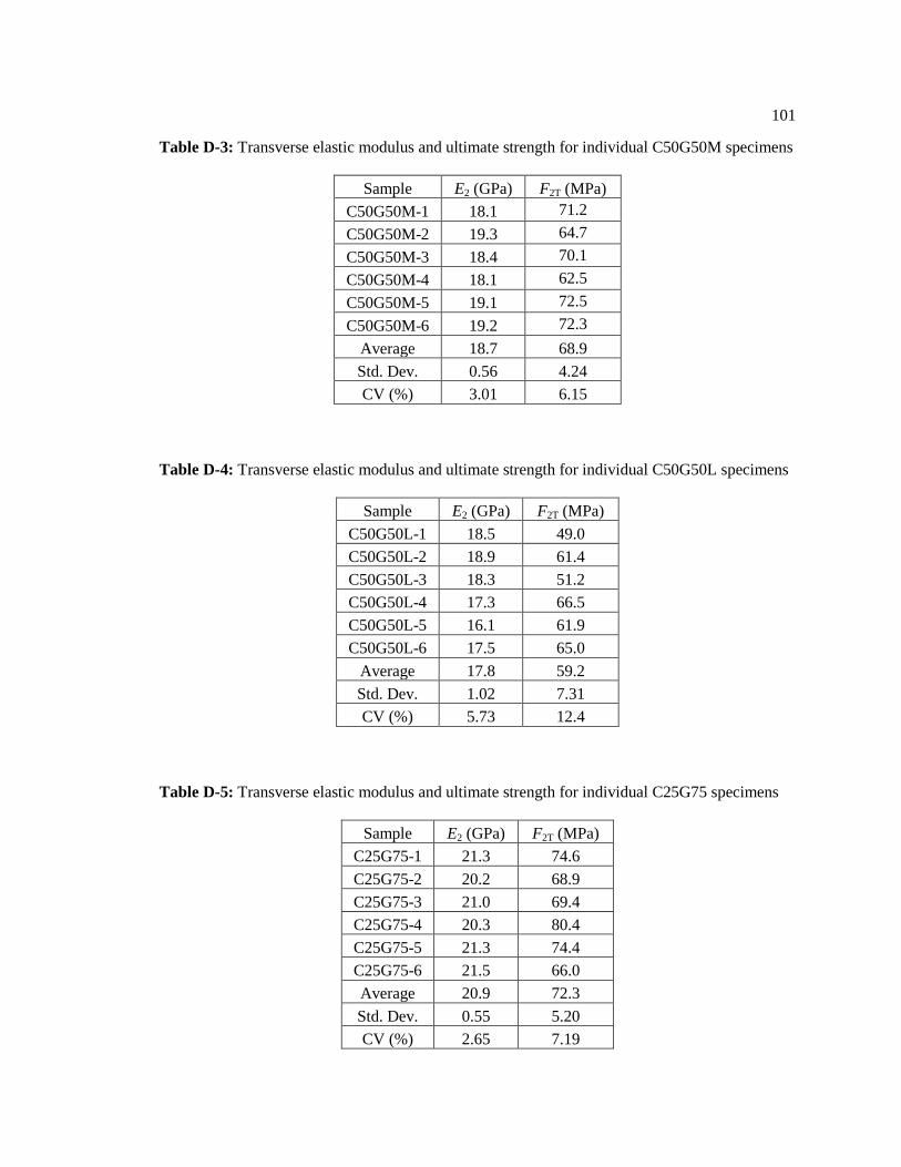
101

Table D-3: Transverse elastic modulus and ultimate strength for individual C50G50M specimens

Sample E2 (GPa) F2T (MPa) C50G50M-1 18.1 71.2 C50G50M-2 19.3 64.7 C50G50M-3 18.4 70.1 C50G50M-4 18.1 62.5 C50G50M-5 19.1 72.5 C50G50M-6 19.2 72.3

Average 18.7 68.9 Std. Dev. 0.56 4.24 CV (%) 3.01 6.15

Table D-4: Transverse elastic modulus and ultimate strength for individual C50G50L specimens

Sample E2 (GPa) F2T (MPa) C50G50L-1 18.5 49.0 C50G50L-2 18.9 61.4 C50G50L-3 18.3 51.2 C50G50L-4 17.3 66.5 C50G50L-5 16.1 61.9 C50G50L-6 17.5 65.0

Average 17.8 59.2 Std. Dev. 1.02 7.31 CV (%) 5.73 12.4

Table D-5: Transverse elastic modulus and ultimate strength for individual C25G75 specimens

Sample E2 (GPa) F2T (MPa) C25G75-1 21.3 74.6 C25G75-2 20.2 68.9 C25G75-3 21.0 69.4 C25G75-4 20.3 80.4 C25G75-5 21.3 74.4 C25G75-6 21.5 66.0 Average 20.9 72.3 Std. Dev. 0.55 5.20 CV (%) 2.65 7.19

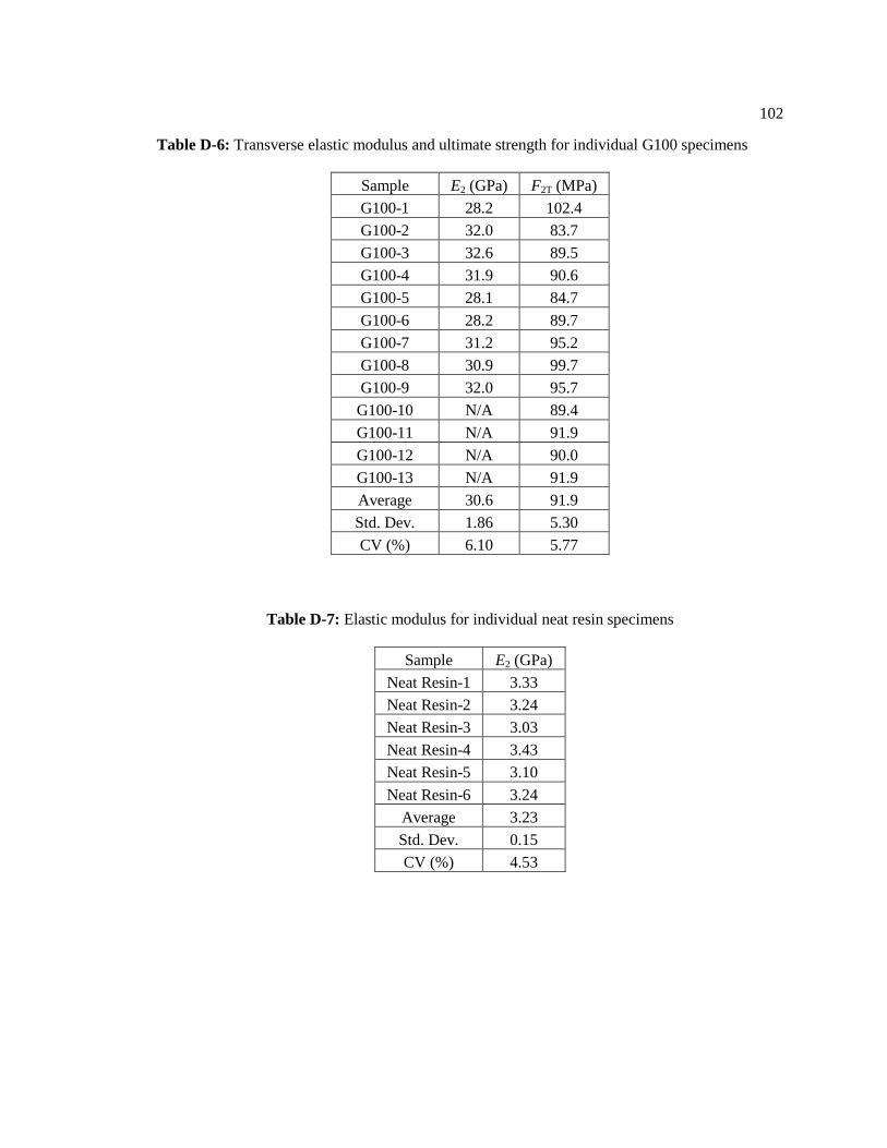
102

Table D-6: Transverse elastic modulus and ultimate strength for individual G100 specimens

Sample E2 (GPa) F2T (MPa) G100-1 28.2 102.4 G100-2 32.0 83.7 G100-3 32.6 89.5 G100-4 31.9 90.6 G100-5 28.1 84.7 G100-6 28.2 89.7 G100-7 31.2 95.2 G100-8 30.9 99.7 G100-9 32.0 95.7

G100-10 N/A 89.4 G100-11 N/A 91.9 G100-12 N/A 90.0 G100-13 N/A 91.9 Average 30.6 91.9 Std. Dev. 1.86 5.30 CV (%) 6.10 5.77

Table D-7: Elastic modulus for individual neat resin specimens

Sample E2 (GPa) Neat Resin-1 3.33 Neat Resin-2 3.24 Neat Resin-3 3.03 Neat Resin-4 3.43 Neat Resin-5 3.10 Neat Resin-6 3.24

Average 3.23 Std. Dev. 0.15 CV (%) 4.53

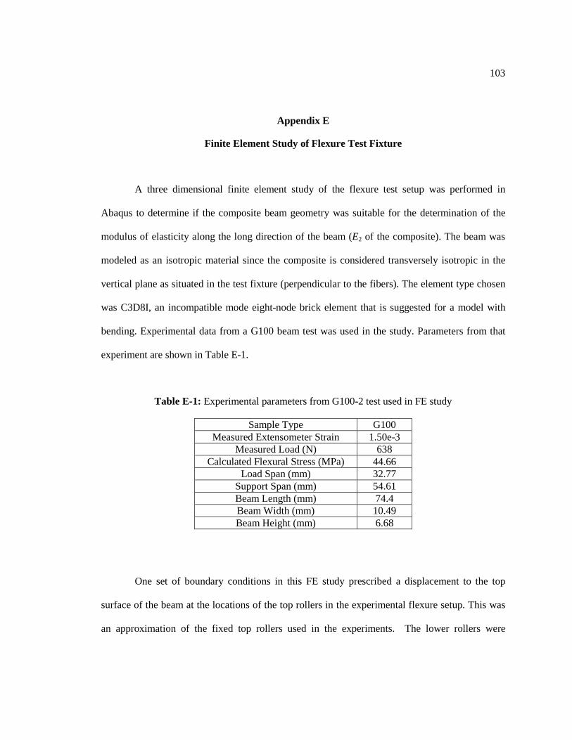
103

Appendix E

Finite Element Study of Flexure Test Fixture

A three dimensional finite element study of the flexure test setup was performed in

Abaqus to determine if the composite beam geometry was suitable for the determination of the

modulus of elasticity along the long direction of the beam (E2 of the composite). The beam was

modeled as an isotropic material since the composite is considered transversely isotropic in the

vertical plane as situated in the test fixture (perpendicular to the fibers). The element type chosen

was C3D8I, an incompatible mode eight-node brick element that is suggested for a model with

bending. Experimental data from a G100 beam test was used in the study. Parameters from that

experiment are shown in Table E-1.

Table E-1: Experimental parameters from G100-2 test used in FE study

Sample Type G100 Measured Extensometer Strain 1.50e-3

Measured Load (N) 638 Calculated Flexural Stress (MPa) 44.66

Load Span (mm) 32.77 Support Span (mm) 54.61 Beam Length (mm) 74.4 Beam Width (mm) 10.49 Beam Height (mm) 6.68

One set of boundary conditions in this FE study prescribed a displacement to the top

surface of the beam at the locations of the top rollers in the experimental flexure setup. This was

an approximation of the fixed top rollers used in the experiments. The lower rollers were

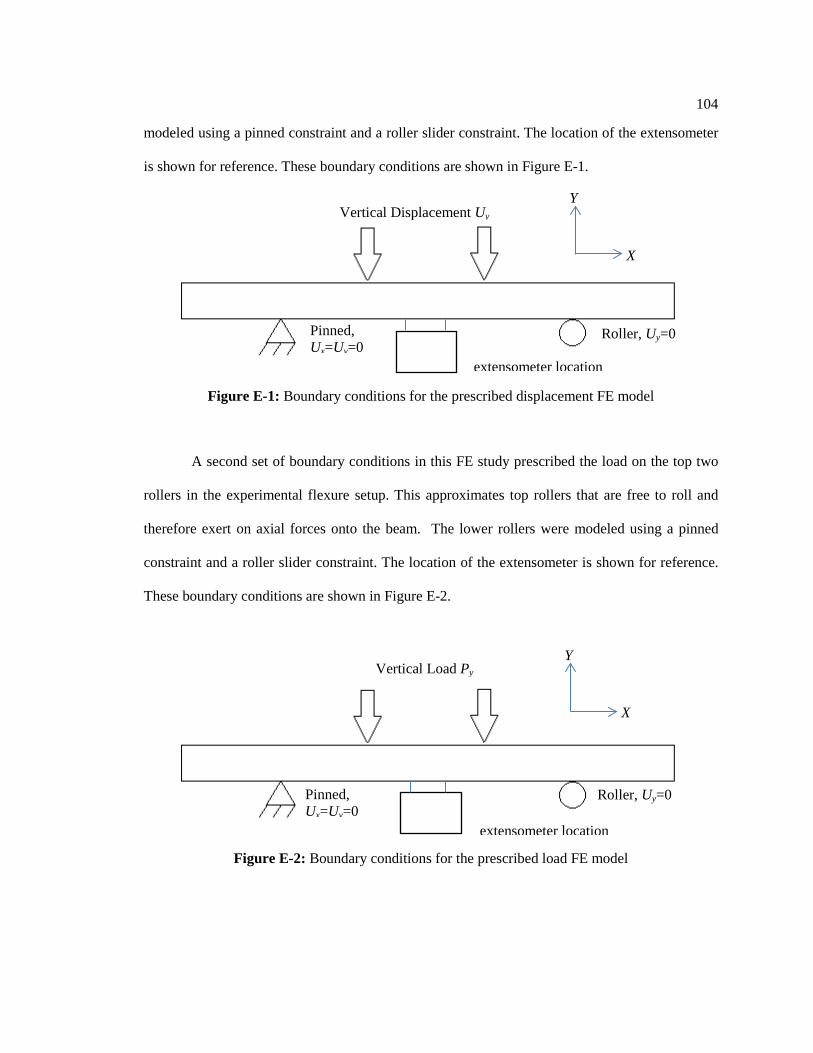
104

modeled using a pinned constraint and a roller slider constraint. The location of the extensometer

is shown for reference. These boundary conditions are shown in Figure E-1.

Figure E-1: Boundary conditions for the prescribed displacement FE model

A second set of boundary conditions in this FE study prescribed the load on the top two

rollers in the experimental flexure setup. This approximates top rollers that are free to roll and

therefore exert on axial forces onto the beam. The lower rollers were modeled using a pinned

constraint and a roller slider constraint. The location of the extensometer is shown for reference.

These boundary conditions are shown in Figure E-2.

Figure E-2: Boundary conditions for the prescribed load FE model

Vertical Displacement Uy

X

Y

Pinned, Ux=Uy=0

Roller, Uy=0

Vertical Load Py

Pinned, Ux=Uy=0

Roller, Uy=0

Y

X

extensometer location

extensometer location

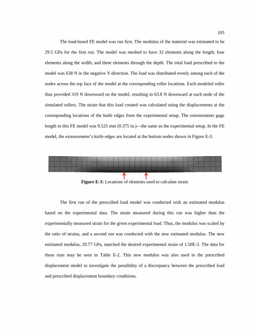
105

The load-based FE model was run first. The modulus of the material was estimated to be

29.5 GPa for the first run. The model was meshed to have 32 elements along the length, four

elements along the width, and three elements through the depth. The total load prescribed to the

model was 638 N in the negative Y-direction. The load was distributed evenly among each of the

nodes across the top face of the model at the corresponding roller locations. Each modeled roller

thus provided 319 N downward on the model, resulting in 63.8 N downward at each node of the

simulated rollers. The strain that this load created was calculated using the displacements at the

corresponding locations of the knife edges from the experimental setup. The extensometer gage

length in this FE model was 9.525 mm (0.375 in.)—the same as the experimental setup. In the FE

model, the extensometer’s knife edges are located at the bottom nodes shown in Figure E-3.

Figure E-3: Locations of elements used to calculate strain

The first run of the prescribed load model was conducted with an estimated modulus

based on the experimental data. The strain measured during this run was higher than the

experimentally measured strain for the given experimental load. Thus, the modulus was scaled by

the ratio of strains, and a second run was conducted with the new estimated modulus. The new

estimated modulus, 29.77 GPa, matched the desired experimental strain of 1.50E-3. The data for

these runs may be seen in Table E-2. This new modulus was also used in the prescribed

displacement model to investigate the possibility of a discrepancy between the prescribed load

and prescribed displacement boundary conditions.

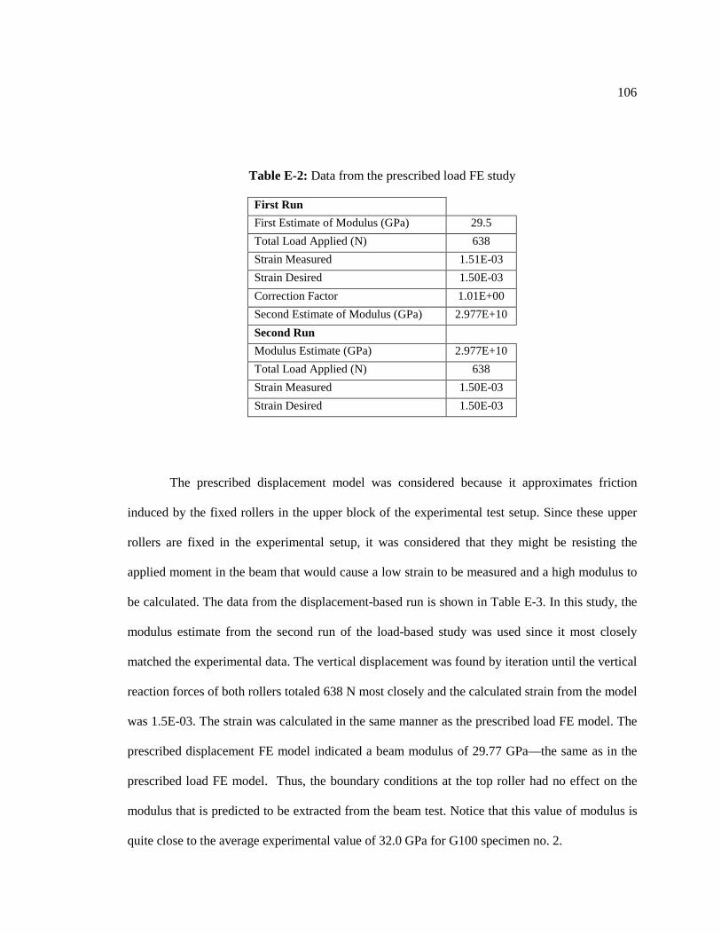
106

Table E-2: Data from the prescribed load FE study

First Run First Estimate of Modulus (GPa) 29.5 Total Load Applied (N) 638 Strain Measured 1.51E-03 Strain Desired 1.50E-03 Correction Factor 1.01E+00 Second Estimate of Modulus (GPa) 2.977E+10 Second Run Modulus Estimate (GPa) 2.977E+10 Total Load Applied (N) 638 Strain Measured 1.50E-03 Strain Desired 1.50E-03

The prescribed displacement model was considered because it approximates friction

induced by the fixed rollers in the upper block of the experimental test setup. Since these upper

rollers are fixed in the experimental setup, it was considered that they might be resisting the

applied moment in the beam that would cause a low strain to be measured and a high modulus to

be calculated. The data from the displacement-based run is shown in Table E-3. In this study, the

modulus estimate from the second run of the load-based study was used since it most closely

matched the experimental data. The vertical displacement was found by iteration until the vertical

reaction forces of both rollers totaled 638 N most closely and the calculated strain from the model

was 1.5E-03. The strain was calculated in the same manner as the prescribed load FE model. The

prescribed displacement FE model indicated a beam modulus of 29.77 GPa—the same as in the

prescribed load FE model. Thus, the boundary conditions at the top roller had no effect on the

modulus that is predicted to be extracted from the beam test. Notice that this value of modulus is

quite close to the average experimental value of 32.0 GPa for G100 specimen no. 2.

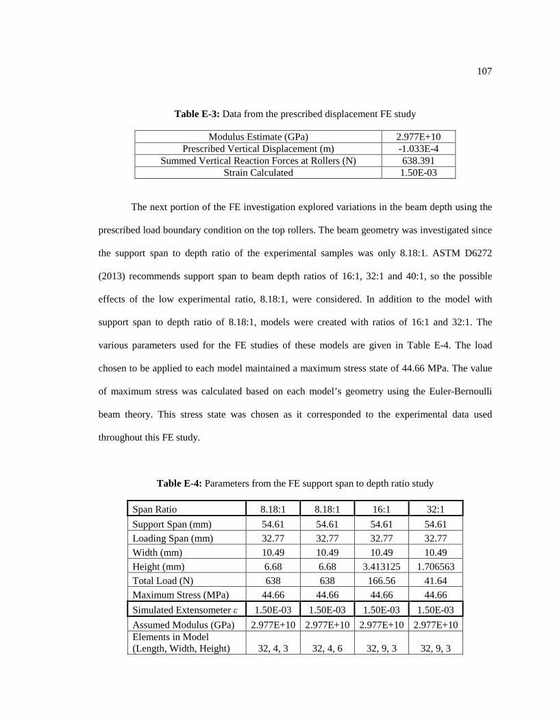
107

Table E-3: Data from the prescribed displacement FE study

Modulus Estimate (GPa) 2.977E+10 Prescribed Vertical Displacement (m) -1.033E-4

Summed Vertical Reaction Forces at Rollers (N) 638.391 Strain Calculated 1.50E-03

The next portion of the FE investigation explored variations in the beam depth using the

prescribed load boundary condition on the top rollers. The beam geometry was investigated since

the support span to depth ratio of the experimental samples was only 8.18:1. ASTM D6272

(2013) recommends support span to beam depth ratios of 16:1, 32:1 and 40:1, so the possible

effects of the low experimental ratio, 8.18:1, were considered. In addition to the model with

support span to depth ratio of 8.18:1, models were created with ratios of 16:1 and 32:1. The

various parameters used for the FE studies of these models are given in Table E-4. The load

chosen to be applied to each model maintained a maximum stress state of 44.66 MPa. The value

of maximum stress was calculated based on each model’s geometry using the Euler-Bernoulli

beam theory. This stress state was chosen as it corresponded to the experimental data used

throughout this FE study.

Table E-4: Parameters from the FE support span to depth ratio study

Span Ratio 8.18:1 8.18:1 16:1 32:1 Support Span (mm) 54.61 54.61 54.61 54.61 Loading Span (mm) 32.77 32.77 32.77 32.77 Width (mm) 10.49 10.49 10.49 10.49 Height (mm) 6.68 6.68 3.413125 1.706563 Total Load (N) 638 638 166.56 41.64 Maximum Stress (MPa) 44.66 44.66 44.66 44.66 Simulated Extensometer ε 1.50E-03 1.50E-03 1.50E-03 1.50E-03 Assumed Modulus (GPa) 2.977E+10 2.977E+10 2.977E+10 2.977E+10 Elements in Model (Length, Width, Height) 32, 4, 3 32, 4, 6 32, 9, 3 32, 9, 3

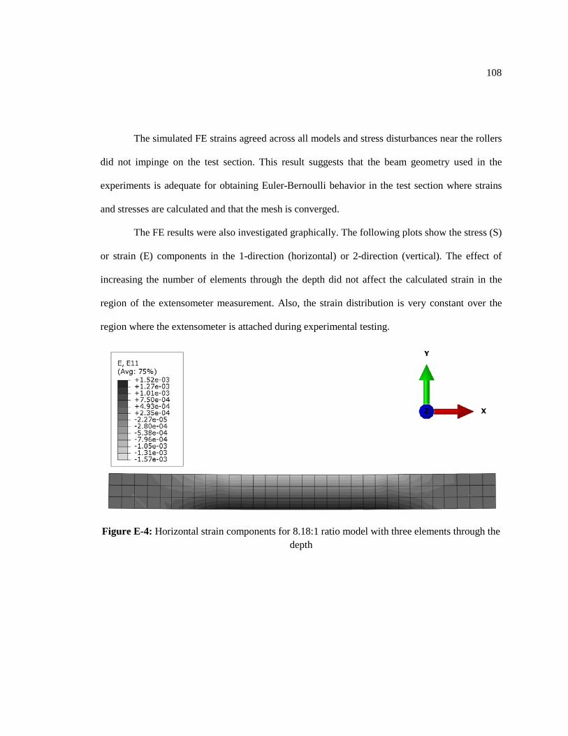
108

The simulated FE strains agreed across all models and stress disturbances near the rollers

did not impinge on the test section. This result suggests that the beam geometry used in the

experiments is adequate for obtaining Euler-Bernoulli behavior in the test section where strains

and stresses are calculated and that the mesh is converged.

The FE results were also investigated graphically. The following plots show the stress (S)

or strain (E) components in the 1-direction (horizontal) or 2-direction (vertical). The effect of

increasing the number of elements through the depth did not affect the calculated strain in the

region of the extensometer measurement. Also, the strain distribution is very constant over the

region where the extensometer is attached during experimental testing.

Figure E-4: Horizontal strain components for 8.18:1 ratio model with three elements through the depth

109

Figure E-5: Horizontal strain components for 8.18:1 ratio model with six elements through the depth

Figure E-6: Vertical strain components for 8.18:1 ratio model with three elements through the depth

110

Figure E-7: Vertical strain components for 8.18:1 ratio model with six elements through the depth

Figure E-8: Horizontal stress components for 8.18:1 ratio model with three elements through the depth

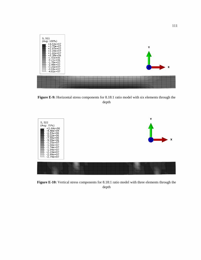
111

Figure E-9: Horizontal stress components for 8.18:1 ratio model with six elements through the depth

Figure E-10: Vertical stress components for 8.18:1 ratio model with three elements through the depth

112

Figure E-11: Vertical stress components for 8.18:1 ratio model with six elements through the depth

Figure E-12: Horizontal strain components for 32:1 ratio model with three elements through the depth

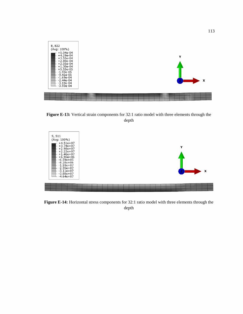
113

Figure E-13: Vertical strain components for 32:1 ratio model with three elements through the depth

Figure E-14: Horizontal stress components for 32:1 ratio model with three elements through the depth

114

Figure E-15: Vertical stress components for 32:1 ratio model with three elements through the depth

Based on the graphical and numerical results from the support span ratio FE study, it was

claimed that the experimental ratio of 8.18:1 was not causing an inflation of the composite

moduli. The region where the extensometer was attached during experimental testing did not

display sensitivity to the different geometries investigated here.

115

Appendix F

Nontechnical Abstract

Fiber reinforced composite materials exhibit excellent material properties along the fiber

direction but are much weaker and less stiff perpendicular to the axis of the fibers. This

phenomenon creates important design considerations when using composites for engineering

applications. This investigation explored the material properties of glass and carbon hybridized

composites perpendicular to the axis of the fibers. Experimental data for these properties did not

previously exist. The composites created for experimental testing were hoop wound rings, where

the continuous fibers run in the circumferential direction throughout the hoop. Four types of

hybridized rings were tested, including the following distributions of glass and carbon fibers

respectively: 25%/75%, 50%/50%, 75%/25%. Two non-hybridized rings were also created for

comparison to the hybrids with 100% carbon and 100% glass fiber reinforcement contents. The

strength and stiffness of each hybrid was tested in flexure by extracting small beams from the

rings. The strength and stiffness of all ring specimens was lowest with the 100% carbon ring, and

highest with the 100% glass ring. The hybrids followed these bounds, and the strength and

stiffness were found to increase in each composite as more glass fiber was present, relative to

carbon fiber. The experimental data were compared to existing analytical models, and some

models were found to correlate well with the use of curve fitting parameters. The experimental

data were also compared to the results from finite element analyses, but the agreement was not

acceptable.