tree-based methods
TRANSCRIPT

Tree-based Methods
• Here we describe tree-based methods for regression andclassification.
• These involve stratifying or segmenting the predictor spaceinto a number of simple regions.
• Since the set of splitting rules used to segment thepredictor space can be summarized in a tree, these types ofapproaches are known as decision-tree methods.
1 / 51

Pros and Cons
• Tree-based methods are simple and useful forinterpretation.
• However they typically are not competitive with the bestsupervised learning approaches in terms of predictionaccuracy.
• Hence we also discuss bagging, random forests, andboosting. These methods grow multiple trees which arethen combined to yield a single consensus prediction.
• Combining a large number of trees can often result indramatic improvements in prediction accuracy, at theexpense of some loss interpretation.
2 / 51

The Basics of Decision Trees
• Decision trees can be applied to both regression andclassification problems.
• We first consider regression problems, and then move on toclassification.
3 / 51

Baseball salary data: how would you stratify it?Salary is color-coded from low (blue, green) to high (yellow,red)
●
●
●
●
●
●
●
●
●
●
●
●
●
●
●
●
●
●
●●
●●
●
●
●
●
●
●
●
●
●
●●
●
●
●
●
●
●
●
●●
●
●
●
●
●
●●
●
●
●
●
●
●
●
●
●●
●
●
●
●
●
●
●
●
●
●
●
●
●
●
●
●●
●
●
●
●
●
●
●
●
●
●
●
●
●
●
●
●
●
●
●
●
●
●
●
●
●
●
●
●●
●
●●
●
●
●
●●
●
●
●
●
●
●
●
●
●
●
●
●
●
●
●
●
●
●
●
●
●
●
●
●
●
●
●
●
●
●
●
●
●
●
●
●
●●
●
●
●
●
●
●
●
●
●
●
●
●
●
●
●
●
●
●●
●
●
●
●
●
●
●
●
●
●
●
●
●
●
●
●
●
●
●●
●
●●
●
●
●
●
●
●
●
●
●
●
●
●
●
●
●
●
●
●
●
●
●
●
●
●
●
●
●
●
●
●
●
●
●
●●
●
●
●
●
●
●
●
●
●
●
●
●
●
●●
●
●
●
●
●
●
●
●
●
●
●
●
●
●
●
●
●
●
●
●
5 10 15 20
050
100
150
200
Years
Hits
4 / 51

Decision tree for these data
|Years < 4.5
Hits < 117.5
5.11
6.00 6.74
5 / 51

Details of previous figure
• For the Hitters data, a regression tree for predicting the logsalary of a baseball player, based on the number of years that hehas played in the major leagues and the number of hits that hemade in the previous year.
• At a given internal node, the label (of the form Xj < tk)indicates the left-hand branch emanating from that split, andthe right-hand branch corresponds to Xj ≥ tk. For instance, thesplit at the top of the tree results in two large branches. Theleft-hand branch corresponds to Years<4.5, and the right-handbranch corresponds to Years>=4.5.
• The tree has two internal nodes and three terminal nodes, orleaves. The number in each leaf is the mean of the response forthe observations that fall there.
6 / 51

Results
• Overall, the tree stratifies or segments the players intothree regions of predictor space: R1 ={X | Years< 4.5},R2 ={X | Years>=4.5, Hits<117.5}, and R3 ={X |Years>=4.5, Hits>=117.5}.
Years
Hits
1
117.5
238
1 4.5 24
R1
R3
R2
7 / 51

Terminology for Trees
• In keeping with the tree analogy, the regions R1, R2, andR3 are known as terminal nodes
• Decision trees are typically drawn upside down, in thesense that the leaves are at the bottom of the tree.
• The points along the tree where the predictor space is splitare referred to as internal nodes
• In the hitters tree, the two internal nodes are indicated bythe text Years<4.5 and Hits<117.5.
8 / 51

Interpretation of Results
• Years is the most important factor in determining Salary,and players with less experience earn lower salaries thanmore experienced players.
• Given that a player is less experienced, the number of Hitsthat he made in the previous year seems to play little rolein his Salary.
• But among players who have been in the major leagues forfive or more years, the number of Hits made in theprevious year does affect Salary, and players who mademore Hits last year tend to have higher salaries.
• Surely an over-simplification, but compared to a regressionmodel, it is easy to display, interpret and explain
9 / 51

Details of the tree-building process
1. We divide the predictor space — that is, the set of possiblevalues for X1, X2, . . . , Xp — into J distinct andnon-overlapping regions, R1, R2, . . . , RJ .
2. For every observation that falls into the region Rj , wemake the same prediction, which is simply the mean of theresponse values for the training observations in Rj .
10 / 51

More details of the tree-building process
• In theory, the regions could have any shape. However, wechoose to divide the predictor space into high-dimensionalrectangles, or boxes, for simplicity and for ease ofinterpretation of the resulting predictive model.
• The goal is to find boxes R1, . . . , RJ that minimize theRSS, given by
J∑j=1
∑i∈Rj
(yi − yRj)2,
where yRjis the mean response for the training
observations within the jth box.
11 / 51

More details of the tree-building process
• Unfortunately, it is computationally infeasible to considerevery possible partition of the feature space into J boxes.
• For this reason, we take a top-down, greedy approach thatis known as recursive binary splitting.
• The approach is top-down because it begins at the top ofthe tree and then successively splits the predictor space;each split is indicated via two new branches further downon the tree.
• It is greedy because at each step of the tree-buildingprocess, the best split is made at that particular step,rather than looking ahead and picking a split that will leadto a better tree in some future step.
12 / 51

Details— Continued
• We first select the predictor Xj and the cutpoint s suchthat splitting the predictor space into the regions{X|Xj < s} and {X|Xj ≥ s} leads to the greatest possiblereduction in RSS.
• Next, we repeat the process, looking for the best predictorand best cutpoint in order to split the data further so as tominimize the RSS within each of the resulting regions.
• However, this time, instead of splitting the entire predictorspace, we split one of the two previously identified regions.We now have three regions.
• Again, we look to split one of these three regions further,so as to minimize the RSS. The process continues until astopping criterion is reached; for instance, we may continueuntil no region contains more than five observations.
13 / 51

Predictions
• We predict the response for a given test observation usingthe mean of the training observations in the region towhich that test observation belongs.
• A five-region example of this approach is shown in the nextslide.
14 / 51

|
t1
t2
t3
t4
R1
R1
R2
R2
R3
R3
R4
R4
R5
R5
X1
X1X1
X2
X2
X2
X1 ≤ t1
X2 ≤ t2 X1 ≤ t3
X2 ≤ t4
15 / 51

Details of previous figure
Top Left: A partition of two-dimensional feature space thatcould not result from recursive binary splitting.
Top Right: The output of recursive binary splitting on atwo-dimensional example.
Bottom Left: A tree corresponding to the partition in the topright panel.
Bottom Right: A perspective plot of the prediction surfacecorresponding to that tree.
16 / 51

Pruning a tree
• The process described above may produce good predictionson the training set, but is likely to overfit the data, leadingto poor test set performance.Why?
• A smaller tree with fewer splits (that is, fewer regionsR1, . . . , RJ) might lead to lower variance and betterinterpretation at the cost of a little bias.
• One possible alternative to the process described above isto grow the tree only so long as the decrease in the RSSdue to each split exceeds some (high) threshold.
• This strategy will result in smaller trees, but is tooshort-sighted: a seemingly worthless split early on in thetree might be followed by a very good split — that is, asplit that leads to a large reduction in RSS later on.
17 / 51

Pruning a tree— continued
• A better strategy is to grow a very large tree T0, and thenprune it back in order to obtain a subtree
• Cost complexity pruning — also known as weakest linkpruning — is used to do this
• we consider a sequence of trees indexed by a nonnegativetuning parameter α. For each value of α there correspondsa subtree T ⊂ T0 such that
|T |∑m=1
∑i: xi∈Rm
(yi − yRm)2 + α|T |
is as small as possible. Here |T | indicates the number ofterminal nodes of the tree T , Rm is the rectangle (i.e. thesubset of predictor space) corresponding to the mthterminal node, and yRm is the mean of the trainingobservations in Rm.
18 / 51

Choosing the best subtree
• The tuning parameter α controls a trade-off between thesubtree’s complexity and its fit to the training data.
• We select an optimal value α using cross-validation.
• We then return to the full data set and obtain the subtreecorresponding to α.
19 / 51

Summary: tree algorithm
1. Use recursive binary splitting to grow a large tree on thetraining data, stopping only when each terminal node hasfewer than some minimum number of observations.
2. Apply cost complexity pruning to the large tree in order toobtain a sequence of best subtrees, as a function of α.
3. Use K-fold cross-validation to choose α. For eachk = 1, . . . ,K:
3.1 Repeat Steps 1 and 2 on the K−1K th fraction of the training
data, excluding the kth fold.3.2 Evaluate the mean squared prediction error on the data in
the left-out kth fold, as a function of α.
Average the results, and pick α to minimize the averageerror.
4. Return the subtree from Step 2 that corresponds to thechosen value of α.
20 / 51

Baseball example continued
• First, we randomly divided the data set in half, yielding132 observations in the training set and 131 observations inthe test set.
• We then built a large regression tree on the training dataand varied α in in order to create subtrees with differentnumbers of terminal nodes.
• Finally, we performed six-fold cross-validation in order toestimate the cross-validated MSE of the trees as a functionof α.
21 / 51

Baseball example continued|
Years < 4.5
RBI < 60.5
Putouts < 82
Years < 3.5
Years < 3.5
Hits < 117.5
Walks < 43.5
Runs < 47.5
Walks < 52.5
RBI < 80.5
Years < 6.5
5.487
4.622 5.183
5.394 6.189
6.015 5.5716.407 6.549
6.459 7.0077.289
22 / 51

Baseball example continued
2 4 6 8 10
0.0
0.2
0.4
0.6
0.8
1.0
Tree Size
Me
an
Sq
ua
red
Err
or
Training
Cross−Validation
Test
23 / 51

Classification Trees
• Very similar to a regression tree, except that it is used topredict a qualitative response rather than a quantitativeone.
• For a classification tree, we predict that each observationbelongs to the most commonly occurring class of trainingobservations in the region to which it belongs.
24 / 51

Details of classification trees
• Just as in the regression setting, we use recursive binarysplitting to grow a classification tree.
• In the classification setting, RSS cannot be used as acriterion for making the binary splits
• A natural alternative to RSS is the classification error rate.this is simply the fraction of the training observations inthat region that do not belong to the most common class:
E = 1−maxk
(pmk).
Here pmk represents the proportion of training observationsin the mth region that are from the kth class.
• However classification error is not sufficiently sensitive fortree-growing, and in practice two other measures arepreferable.
25 / 51

Gini index and Deviance• The Gini index is defined by
G =
K∑k=1
pmk(1− pmk),
a measure of total variance across the K classes. The Giniindex takes on a small value if all of the pmk’s are close tozero or one.
• For this reason the Gini index is referred to as a measure ofnode purity — a small value indicates that a node containspredominantly observations from a single class.
• An alternative to the Gini index is cross-entropy, given by
D = −K∑k=1
pmk log pmk.
• It turns out that the Gini index and the cross-entropy arevery similar numerically.
26 / 51

Example: heart data
• These data contain a binary outcome HD for 303 patientswho presented with chest pain.
• An outcome value of Yes indicates the presence of heartdisease based on an angiographic test, while No means noheart disease.
• There are 13 predictors including Age, Sex, Chol (acholesterol measurement), and other heart and lungfunction measurements.
• Cross-validation yields a tree with six terminal nodes. Seenext figure.
27 / 51

|Thal:a
Ca < 0.5
MaxHR < 161.5
RestBP < 157
Chol < 244MaxHR < 156
MaxHR < 145.5
ChestPain:bc
Chol < 244 Sex < 0.5
Ca < 0.5
Slope < 1.5
Age < 52 Thal:b
ChestPain:a
Oldpeak < 1.1
RestECG < 1
No YesNo
NoYes
No
No No No Yes
Yes No No
No Yes
Yes Yes
Yes
5 10 15
0.0
0.1
0.2
0.3
0.4
0.5
0.6
Tree Size
Err
or
TrainingCross−ValidationTest
|Thal:a
Ca < 0.5
MaxHR < 161.5 ChestPain:bc
Ca < 0.5
No No
No Yes
Yes Yes
28 / 51

Trees Versus Linear Models
−2 −1 0 1 2
−2
−1
01
2
X1
X2
−2 −1 0 1 2
−2
−1
01
2
X1
X2
−2 −1 0 1 2
−2
−1
01
2
X1
X2
−2 −1 0 1 2
−2
−1
01
2
X1
X2
Top Row: True linear boundary; Bottom row: true non-linearboundary.
Left column: linear model; Right column: tree-based model
29 / 51

Advantages and Disadvantages of Trees
s Trees are very easy to explain to people. In fact, they areeven easier to explain than linear regression!
s Some people believe that decision trees more closely mirrorhuman decision-making than do the regression andclassification approaches seen in previous chapters.
s Trees can be displayed graphically, and are easilyinterpreted even by a non-expert (especially if they aresmall).
s Trees can easily handle qualitative predictors without theneed to create dummy variables.
t Unfortunately, trees generally do not have the same level ofpredictive accuracy as some of the other regression andclassification approaches seen in this book.
However, by aggregating many decision trees, the predictiveperformance of trees can be substantially improved. Weintroduce these concepts next.
30 / 51

Bagging
• Bootstrap aggregation, or bagging, is a general-purposeprocedure for reducing the variance of a statistical learningmethod; we introduce it here because it is particularlyuseful and frequently used in the context of decision trees.
• Recall that given a set of n independent observationsZ1, . . . , Zn, each with variance σ2, the variance of the meanZ of the observations is given by σ2/n.
• In other words, averaging a set of observations reducesvariance. Of course, this is not practical because wegenerally do not have access to multiple training sets.
31 / 51

Bagging— continued
• Instead, we can bootstrap, by taking repeated samplesfrom the (single) training data set.
• In this approach we generate B different bootstrappedtraining data sets. We then train our method on the bthbootstrapped training set in order to get f∗b(x), theprediction at a point x. We then average all the predictionsto obtain
fbag(x) =1
B
B∑b=1
f∗b(x).
This is called bagging.
32 / 51

Bagging classification trees
• The above prescription applied to regression trees
• For classification trees: for each test observation, we recordthe class predicted by each of the B trees, and take amajority vote: the overall prediction is the most commonlyoccurring class among the B predictions.
33 / 51

Bagging the heart data
0 50 100 150 200 250 300
0.10
0.15
0.20
0.25
0.30
Number of Trees
Err
or
Test: BaggingTest: RandomForestOOB: BaggingOOB: RandomForest
34 / 51

Details of previous figure
Bagging and random forest results for the Heart data.
• The test error (black and orange) is shown as a function ofB, the number of bootstrapped training sets used.
• Random forests were applied with m =√p.
• The dashed line indicates the test error resulting from asingle classification tree.
• The green and blue traces show the OOB error, which inthis case is considerably lower
35 / 51

Out-of-Bag Error Estimation
• It turns out that there is a very straightforward way toestimate the test error of a bagged model.
• Recall that the key to bagging is that trees are repeatedlyfit to bootstrapped subsets of the observations. One canshow that on average, each bagged tree makes use ofaround two-thirds of the observations.
• The remaining one-third of the observations not used to fita given bagged tree are referred to as the out-of-bag (OOB)observations.
• We can predict the response for the ith observation usingeach of the trees in which that observation was OOB. Thiswill yield around B/3 predictions for the ith observation,which we average.
• This estimate is essentially the LOO cross-validation errorfor bagging, if B is large.
36 / 51

Random Forests
• Random forests provide an improvement over bagged treesby way of a small tweak that decorrelates the trees. Thisreduces the variance when we average the trees.
• As in bagging, we build a number of decision trees onbootstrapped training samples.
• But when building these decision trees, each time a split ina tree is considered, a random selection of m predictors ischosen as split candidates from the full set of p predictors.The split is allowed to use only one of those m predictors.
• A fresh selection of m predictors is taken at each split, andtypically we choose m ≈ √p — that is, the number ofpredictors considered at each split is approximately equalto the square root of the total number of predictors (4 outof the 13 for the Heart data).
37 / 51

Example: gene expression data
• We applied random forests to a high-dimensional biologicaldata set consisting of expression measurements of 4,718genes measured on tissue samples from 349 patients.
• There are around 20,000 genes in humans, and individualgenes have different levels of activity, or expression, inparticular cells, tissues, and biological conditions.
• Each of the patient samples has a qualitative label with 15different levels: either normal or one of 14 different types ofcancer.
• We use random forests to predict cancer type based on the500 genes that have the largest variance in the training set.
• We randomly divided the observations into a training and atest set, and applied random forests to the training set forthree different values of the number of splitting variables m.
38 / 51

Results: gene expression data
0 100 200 300 400 500
0.2
0.3
0.4
0.5
Number of Trees
Test C
lassific
ation E
rror
m=p
m=p/2
m= p
39 / 51

Details of previous figure
• Results from random forests for the fifteen-class geneexpression data set with p = 500 predictors.
• The test error is displayed as a function of the number oftrees. Each colored line corresponds to a different value ofm, the number of predictors available for splitting at eachinterior tree node.
• Random forests (m < p) lead to a slight improvement overbagging (m = p). A single classification tree has an errorrate of 45.7%.
40 / 51

Boosting
• Like bagging, boosting is a general approach that can beapplied to many statistical learning methods for regressionor classification. We only discuss boosting for decisiontrees.
• Recall that bagging involves creating multiple copies of theoriginal training data set using the bootstrap, fitting aseparate decision tree to each copy, and then combining allof the trees in order to create a single predictive model.
• Notably, each tree is built on a bootstrap data set,independent of the other trees.
• Boosting works in a similar way, except that the trees aregrown sequentially: each tree is grown using informationfrom previously grown trees.
41 / 51

Boosting algorithm for regression trees
1. Set f(x) = 0 and ri = yi for all i in the training set.
2. For b = 1, 2, . . . , B, repeat:
2.1 Fit a tree f b with d splits (d+ 1 terminal nodes) to thetraining data (X, r).
2.2 Update f by adding in a shrunken version of the new tree:
f(x)← f(x) + λf b(x).
2.3 Update the residuals,
ri ← ri − λf b(xi).
3. Output the boosted model,
f(x) =
B∑b=1
λf b(x).
42 / 51

What is the idea behind this procedure?
• Unlike fitting a single large decision tree to the data, whichamounts to fitting the data hard and potentially overfitting,the boosting approach instead learns slowly.
• Given the current model, we fit a decision tree to theresiduals from the model. We then add this new decisiontree into the fitted function in order to update theresiduals.
• Each of these trees can be rather small, with just a fewterminal nodes, determined by the parameter d in thealgorithm.
• By fitting small trees to the residuals, we slowly improve fin areas where it does not perform well. The shrinkageparameter λ slows the process down even further, allowingmore and different shaped trees to attack the residuals.
43 / 51

Boosting for classification
• Boosting for classification is similar in spirit to boosting forregression, but is a bit more complex. We will not go intodetail here, nor do we in the text book.
• Students can learn about the details in Elements ofStatistical Learning, chapter 10.
• The R package gbm (gradient boosted models) handles avariety of regression and classification problems.
44 / 51

Gene expression data continued
0 1000 2000 3000 4000 5000
0.0
50.1
00.1
50.2
00.2
5
Number of Trees
Test C
lassific
ation E
rror
Boosting: depth=1
Boosting: depth=2
RandomForest: m= p
45 / 51
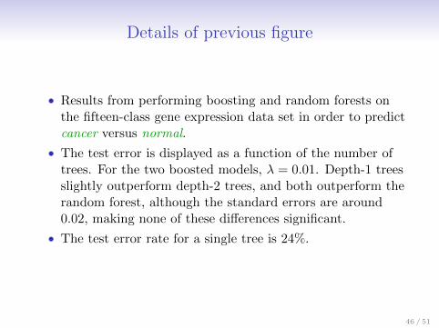
Details of previous figure
• Results from performing boosting and random forests onthe fifteen-class gene expression data set in order to predictcancer versus normal.
• The test error is displayed as a function of the number oftrees. For the two boosted models, λ = 0.01. Depth-1 treesslightly outperform depth-2 trees, and both outperform therandom forest, although the standard errors are around0.02, making none of these differences significant.
• The test error rate for a single tree is 24%.
46 / 51

Tuning parameters for boosting
1. The number of trees B. Unlike bagging and random forests,boosting can overfit if B is too large, although thisoverfitting tends to occur slowly if at all. We usecross-validation to select B.
2. The shrinkage parameter λ, a small positive number. Thiscontrols the rate at which boosting learns. Typical valuesare 0.01 or 0.001, and the right choice can depend on theproblem. Very small λ can require using a very large valueof B in order to achieve good performance.
3. The number of splits d in each tree, which controls thecomplexity of the boosted ensemble. Often d = 1 workswell, in which case each tree is a stump, consisting of asingle split and resulting in an additive model. Moregenerally d is the interaction depth, and controls theinteraction order of the boosted model, since d splits caninvolve at most d variables.
47 / 51

Another regression example
0 200 400 600 800 1000
0.32
0.34
0.36
0.38
0.40
0.42
0.44
California Housing Data
Number of Trees
Tes
t Ave
rage
Abs
olut
e E
rror
RF m=2RF m=6GBM depth=4GBM depth=6
from Elements of Statistical Learning, chapter 15.
48 / 51

Another classification example
0 500 1000 1500 2000 2500
0.04
00.
045
0.05
00.
055
0.06
00.
065
0.07
0
Spam Data
Number of Trees
Tes
t Err
orBaggingRandom ForestGradient Boosting (5 Node)
from Elements of Statistical Learning, chapter 15.
49 / 51

Variable importance measure• For bagged/RF regression trees, we record the total
amount that the RSS is decreased due to splits over a givenpredictor, averaged over all B trees. A large value indicatesan important predictor.
• Similarly, for bagged/RF classification trees, we add up thetotal amount that the Gini index is decreased by splits overa given predictor, averaged over all B trees.
Thal
Ca
ChestPain
Oldpeak
MaxHR
RestBP
Age
Chol
Slope
Sex
ExAng
RestECG
Fbs
0 20 40 60 80 100
Variable Importance
Variable importance plotfor the Heart data
50 / 51

Summary
• Decision trees are simple and interpretable models forregression and classification
• However they are often not competitive with othermethods in terms of prediction accuracy
• Bagging, random forests and boosting are good methodsfor improving the prediction accuracy of trees. They workby growing many trees on the training data and thencombining the predictions of the resulting ensemble of trees.
• The latter two methods— random forests and boosting—are among the state-of-the-art methods for supervisedlearning. However their results can be difficult to interpret.
51 / 51