tree encoding in the itu-t g.711.1 speech coder · tree encoding in the itu -t g.711.1 spee ch...

2010/11/28

Tree Encoding in the ITU-T

G.711.1 Speech Coder

Abdul Hannan Khan

Department of Electrical Computer and Software Engineering

McGill University

Montreal, Canada

November, 2010

A thesis submitted to McGill University in partial fulfillment of the requirements for

the degree of Master of Engineering

© 2010 Abdul Hannan Khan

Tree Encoding in the ITU-T G.711.1 Speech

Coder

2010

i

ABSTRACT

This thesis examines further enhancement to ITU-T G.711.1 speech coder.

The original G.711 coder is effectively a low band �-law quantizer. The G.711.1

extension adds noise feed-back and lower band enhancement layer apart from the

higher-band. To further improve the core lower-band coding performance the use of

both vector quantization and delayed decision multi-path tree encoder in the above

coder at the low band portion is studied. The delayed decision multi-path tree

encoding is implemented by the (�, �) – algorithm. The new quantizer takes into

account past history, and hence, the error propagation due to noise feed-back, and

codes multiple samples under �-law. The final bitstream is compatible with the

G.711.1 decoder and, hence, with the original G.711 decoder. An evaluation method,

ITU-T P.862 perceptual evaluation of speech quality (PESQ), is used to evaluate the

performance. Both the vector quantizer and tree encoder have better performance

than the original core layer encoder in terms of perceptual quality, though they are

limited by the increased computational complexity. Future studies are suggested.


Coder

2010

ii

SOMMAIRE

Cette thèse étudie en détail les améliorations apportées au codeur de la

parole ITU-T G.711.1. Le codeur original G.711 est en fait un quantificateur�-law. Le

prolongement large-bande G.711.1 utilise le façonnage du bruit ainsi qu’une couche

d’amélioration de la bande-basse en plus de la bande-haute. Afin d’améliorer le

codage de la bande-basse principale, nous étudions l’utilisation de quantification

vectorielle et la décision à retardement. Le codeur arboriforme avec décision à

retardée est réalisé par l’algorithme(�, �). Le nouveau quantificateur considère

l’information passée et par conséquent, il considère également la propagation de

l’erreur engendrée par le façonnage du bruit. Il code plusieurs échantillons par �-

law. Le flot binaire final est compatible avec le décodeur du prolongement large-

bande G.711.1 et donc naturellement avec le décodeur du G.711 original. Une

méthode d’évaluation, ITU-T P.862 (PESQ) est utilisée pour évaluer la performance.

Les résultats montrent que la quantification vectorielle et le codeur arboriforme

sont perceptuellement plus performants que le codeur original de la bande

principale. Nous notons tout de même qu’ils sont numériquement plus complexes à

réaliser. Des études supplémentaires sont suggérées.


Coder

2010

iii

ACKNOWLEDGEMENTS

I would like to thank Dr. Peter Kabal for his continued guidance, supervision,

friendliness and wise counsel throughout the course of this study. I’m grateful to my

family, especially my parents, for their continuous encouragement and support. Also

I thank Mr. Mohamed Konate for translating the abstract of this thesis into French.

Finally, I would like to thank McGill University and its staff for all the resources

provided that were used during the period of this study.


Coder

2010

iv

TABLE OF CONTENTS

Abstract......................................................................................................................................................... i

Sommaire ................................................................................................................................................... ii

Acknowledgements ............................................................................................................................... iii

Table of Contents ................................................................................................................................... iv

List of Figures .......................................................................................................................................... vi

List of Tables ........................................................................................................................................... vii

Chapter 1 Introduction ......................................................................................................................... 1

Chapter 2 ITU-T G.711.1....................................................................................................................... 7

2.1.1 Core Layer ............................................................................................................................ 10

2.1.2 �-law Quantizer ................................................................................................................. 10

2.1.3 Noise Feedback .................................................................................................................. 12

2.1.4 Dead-Zone Quantizer ....................................................................................................... 17

Chapter 3 CELP and Vector Quantization in ADPCM .............................................................. 20

3.1 DPCM .............................................................................................................................................. 21

3.2 ADPCM ........................................................................................................................................... 22

3.3 CELP ............................................................................................................................................... 23

3.4 Vector Quantization in ADPCM ............................................................................................ 25

Chapter 4 Delayed Decision Coding ............................................................................................... 29


Coder

2010

v

4.1 Tree Encoding ............................................................................................................................. 30

4.1.1 Single Path Tree Encoding ............................................................................................. 30

4.1.2 Multi-Path Tree Encoding: The (�, �)—Algorithm ............................................. 32

4.2 Cumulative Error ....................................................................................................................... 36

4.3 Modification to G.711.1 Core Layer .................................................................................... 37

Chapter 5 Computer Simulation ..................................................................................................... 40

5.1 Sub Optimal Approach to Reduce Complexity ............................................................... 40

5.2 Initialization of The System .................................................................................................. 44

5.3 Simulation Inputs ...................................................................................................................... 45

5.4 Performance ................................................................................................................................ 45

5.4.1 Perceptual Evaluation of Speech Quality ................................................................. 45

5.4.2 Comparison with G.711.1 ............................................................................................... 46

5.4.3 Performance as a Function of � .................................................................................. 49

5.4.4 Performance as a Function of � ................................................................................... 51

Chapter 6 Conclusion .......................................................................................................................... 54

References ............................................................................................................................................... 56


Coder

2010

vi

LIST OF FIGURES

Figure 2-1 – Block diagram of G.711.1 encoder .......................................................................... 9

Figure 2-2 – Lower-band encoder .................................................................................................. 10

Figure 2-3 – Noise shaping ................................................................................................................ 12

Figure 2-4 – Quantization noise without noise feedback (left) and with noise

feedback (right) [4] .............................................................................................................................. 16


feedback (right) [2] .............................................................................................................................. 19

Figure 3-1 – DPCM Coding; encoder on the left, decoder on the right ............................. 21

Figure 3-2 – ADPCM encoder block diagram ............................................................................. 22

Figure 3-3 – CELP Encoder................................................................................................................ 24

Figure 3-4 – Rearranged ADPCM encoder structure to show noise feedback .............. 25

Figure 3-5 – VQ in ADPCM encoder with noise feedback ...................................................... 26

Figure 3-6 – VQ in ADPCM encoder with noise feedback – form 1 .................................... 28

Figure 3-7 – VQ in ADPCM encoder with noise feedback – form 2 .................................... 28

Figure 4-1 – Single path tree encoding ......................................................................................... 32

Figure 4-2 – Multi-path tree encoding .......................................................................................... 33

Figure 4-3 – G.711.1 core layer with codebook VQ ................................................................. 38

Figure 4-4 – G.711.1 core layer with codebook VQ - rearranged ....................................... 38

Figure 5-1 – PESQ score of tree encoding as a function of M, with L=6 at -40 dB. For

the first point M=1 and L=1. The performance of G.711.1 core layer is provided for

comparison. ............................................................................................................................................. 50


Coder

2010

vii

Figure 5-2 – PESQ score of tree encoding as a function of L, with M=6 at -40 dB. For

the first point L=1 and M=1. The performance of G.711.1 core layer is provided for

comparison. ............................................................................................................................................. 52

LIST OF TABLES

Table 5-1 – Multiplication and addition operations per sample of different G.711.1

encoders ................................................................................................................................................... 43

Table 5-2 – Comparison of different G.711.1 encoders using PESQ ................................. 47


Coder

2010

1

Chapter 1 INTRODUCTION

Speech coding is the process by which an analog speech signal, continuous in

both time and amplitude, is digitized, i.e. converted to a speech signal discrete in

both time and amplitude. The signal in the process is compressed, hence, taking

fewer resources for storage and/or transmission. Speech coding has some

differences with audio coding. More established models are available for speech as

compared to other audio signals. Psychoacoustics also plays its role in speech

coding. Speech is coded and transmitted such that only information relevant to the

human auditory system is transmitted. Higher quality at a lower bit rate can be

further achieved by making use of signal redundancy and masking the distortions

created by coding such that they become imperceptible. Even a narrow band

(< 4,000Hz) signal is enough for intelligibility. It needs to be clarified that

intelligibility is different from pleasantness. Understanding of the content, speaker

identity, timbre and tone are all vital for the former. Pleasantness is about whether

the degraded speech signal is subjectively irritating or not.


Coder

2010

2

The immediate advantage of speech coding comes in the form of reduced data

storage capacity required. High quality speech can now be stored on a physical

media without consumption of a lot of memory space. Once speech is coded it can be

transmitted as data, utilizing the same public switched loop circuits. Voice and data

signals can be sent on the same channel. Digital speech signals allow better security.

They can be encrypted and/or scrambled with greater efficiency. High quality at low

bit rates have made it possible to meet growing demands of wireless

communication. Today high quality speech coding is available at 8kbps, although

this thesis deals with a speech coder working at 64 kbps or more.

There are different parameters of speech coder performance. The aim of a

speech coder is to improve the speech quality while reducing the bit rate,

communication delay and complexity. The five-point scale on which speech quality

is mostly evaluated is known as the mean-opinion score (MOS) scale. It is a

subjective test and is averaged over a large set of data, speakers and listeners. Scores

of 3.5 or higher are generally considered to have good levels of intelligibility.

Another similar scale based on comparison of the original and degenerated signal is

the perceptual evaluation of sound quality (PESQ). PESQ is an objective measure of

sound quality. Hence, the requirement of having a large set of listeners is eliminated

while the scale is similar. There will always be a slight communication delay as

speech coders have to process data, and they often work in blocks of samples. The

constraint on communication delay is application dependent. Even in real time

communication it varies from 1 to 500��; higher delays are permissible in video


Coder

2010

3

telephony. Complexity is measured in terms of number of arithmetic operations

performed and memory requirements. Higher complexity often results in higher

communication delays and in higher power consumption. With advancements in

chip design technology higher complexity speech coders can now be implemented

with acceptable delays and power consumption.

Generally speech coders are divided into three classes; waveform coders,

source coders and hybrid coders. Waveform coders are the simplest to implement,

from a complexity point of view. They are largely independent of the input signal

and try to reconstruct a signal whose waveform is as close to the input. For a time

domain coding approach the simplest coder involves sampling and quantizing the

input signal. One coder who works on this principle is the pulse code modulation

(PCM) coder. Logarithmic quantization is used to provide same quality of

reconstruction at a reduced bit rate. Such a coder has a bit rate of 64kbps. Another

example of a waveform coder is the differential pulse code modulation (DPCM)

coder. The difference between the input signal and the predicted signal is coded.

This reduces the number of bits required for coding. A typical bit rate for such a

coder is 32kbps. In frequency domain waveform coding, a signal is divided up into

different bands and each is coded and transmitted individually. Examples of such

frequency domain waveform coding are sub-band coding (SBC) and adaptive

transform coding (ATC). These coding techniques are a bit more complex than time

domain coding techniques because of the filtering required to split the input signal

into sub-bands.


Coder

2010

4

Sources coders are typically the lower bit rate coders. Source coders try to

model the source of the input signal. The parameters of the source model are then

transmitted. A time-varying filter is used to model the vocal tract. The excitation

signal depends on whether the input is voiced or unvoiced speech. In the case of the

former a train of pulses is used while for the latter white noise is used. The period of

the pulses is the same as the pitch period of the voiced speech. Filter coefficients,

gain factors, voiced/unvoiced speech decision and pitch period are the parameters

transmitted. There is usually a loss of naturalness in the reconstructed speech from

a source coder. The reconstructed speech has a synthetic feel but this may be

acceptable where low bit rate is preferred over naturalness of speech. Linear

predictive coding (LPC) coder is an example of such a source coder. It operates

around 2.4kbps.

Hybrid coders, as the name suggests, tend to find a compromise between

waveform coders and sources coders, both in terms of how they code the signal and

the bit rate. One of the most important hybrid coders is the code excited linear

predictive (CELP) coder. It is an analysis-by-synthesis coder. It employs linear

prediction and then quantizes the residual signal. The parameters of the linear

prediction filter and the quantized residual signal are transmitted. The residual

signal is used to excite the synthesis filter in the receiver. The quantization of the

residual signal is such that to minimize the error and match the input signal as

closely as possible. Operating between 4.8 and 16 kbps, these coders produce good

quality reconstructed speech.


Coder

2010

5

This thesis presents work done on a speech coder. ITU-T standard G.711.1 is

a wideband embedded extension to G.711 PCM encoded speech [2]. The extension

was approved in March 2008. The G.711.1 wideband extension adds noise feedback

and a lower-band enhancement layer, as well as a high band encoding layer. The

noise feedback tries to perceptually mask the quantization noise introduced by the

PCM quantizer. The perceptual filter is based on the linear prediction filter. What the

enhancement layer does is that it allows more bits to be used for encoding, hence,

increasing the number of quantization levels. This reduces the quantization noise at

the expense of more bits. The higher band encoding is based on modified discrete

cosine transform (MDCT) and uses an interleave conjugate-structure vector

quantizer (CSVQ). This thesis will be talking about the lower-band.

This research studies the effect on G.711.1 speech coder by incorporating

vector quantization (VQ) and delayed decision multi-path tree encoding. While

G.711.1 is concerned with both low and high bands, this thesis concerns only with

the low band. The delayed decision multi-path tree encoding is implemented by the

(�, �)–algorithm as suggested in [3]. � is the maximum number of tree paths

available after quantizing a block of input samples and � is the maximum depth of

the tree. � also dictates the delay after which an input block is coded. Because the

noise feedback filter has memory, a decision made at a certain instance has effect on

decisions made in the future. The new quantizer takes into account past history (or

future values, depending on how you look at it ), and hence, the error propagation

due to noise feedback is taken into consideration as well when making the final


Coder

2010

6

decision on the code. One major advantage is that the final bit-stream is compatible

with the G.711.1 decoder.

The working of the G711.1 speech coder is studied in Chapter 2. The lower-

band quantizer and the noise feedback filter are discussed in detail as these are

common to the new coder; the delayed decision multi-path tree encoding is

implemented in the lower-band. Chapter 3 deals with CELP and adaptive differential

pulse code modulation (ADPCM), as it is from there that the idea of using vector

quantization in G.711.1 originated. Chapter 4 describes delayed decision coding,

multi-path tree encoding to be precise, in detail. Simulation results are provided in

Chapter 5. With Chapter 6 this thesis is concluded.


Coder

2010

7

Chapter 2 ITU-T G.711.1

ITU-T G.711.1’s predecessor, G.711, uses PCM with logarithmic quantization.

With a logarithmic scale, 12 bits of resolution can be achieved by using only 8 bits

per sample. Two such scales exist, �-law and �-law. Except for slight differences in

quantization levels both are essentially the same. In this thesis �-law has been used

and all further mention should be taken as such unless stated otherwise. These

algorithms provide good quality speech coding at very low complexity while saving

33% bandwidth as compared to linear quantization. These properties found them

use in digital telephony and have not been replaced. In 2008 ITU-T recommended a

wideband extension to G.711, ITU-T G.711.1 wideband embedded extension for PCM

[2]. The new coder has an embedded structure and is backward compatible with

existing G.711 coders.

The conventional G.711 log companded PCM encoder has bandwidth of 300—3400

Hz at 64 kbps, and takes input sampled at 8kHz. In G.711.1 all these values have

been increased. For input sampled at 16kHz it has a bandwidth of 50—7000Hz at

80 and 96kbps, while for signal sampled at 8kHz it has a bandwidth of 0—4000Hz


Coder

2010

8

at 64 and 80kbps. Different bit rates are available because of the embedded

structure. The new standard has three layers:

• Core layer (Layer 0): always present at 64kbps

• Lower-band enhancement layer (Layer 1): optional with addition of 16kbps

• Higher-band layer (Layer 2): optional with addition of 16kbps

The core layer, at 64 kbps, is compatible with G.711 decoder. Different combination

of these three layers gives rise to four different encoding modes.

• R1: only core layer at a sampling rate of 8kHz and bit rate of 64kbps

• R2a: core layer and lower-band enhancement layer at a sampling rate

of8kHz and bit rate of 80kbps

• R2b: core layer and higher-band layer at a sampling rate of 16kHz and bit

rate of 80kbps

• R3: all three layers at a sampling rate of 16kHz and bit rate of 96kbps

Figure 2-1 gives a higher level look at the G.711.1 encoder. The wideband input

signal sampled at 16kHz is split by a 32-tap quadrature mirror filterbank (QMF).

The lower-band encoding produces two streams; the G.711 compatible core layer

and the lower-band enhancement layer. MDCT is applied to the higher-band signal

and the frequency domain coefficients are encoded by a CSVQ. The final bitstream is

a multiplexed version of all three. In the case of 8 kHz sampled input signal the QMF

is by-passed and the signal fed directly to the lower-band encoders. It is to be noted


Coder

2010

9

that these input signals have been pre-processed by a high-pass filter with a cut-off

frequency of 50Hz.

2.1 LOWER-BAND ENCODING

In the lower-band, G.711.1 not only adds noise feedback with perceptual

noise shaping to the log companded PCM encoder of G.711, but also an optional

enhancement layer to refine the quantization. A local Layer 0 decoder has been

added to the design. The locally decoded signal is used for the calculation of the

perceptual filter, which then filters the difference between the input signal and the

decoded signal. This perceptually shaped noise is then added to the input signal. The

resulting signal is quantized by the Layer 0 quantizer and the Layer 0 bitstream is

obtained. A refinement signal is sent to the Layer 1 quantizer which generates the

Analysis

QMF

Lower-band

signal Lower-band

embedded PCM

encoders

Core layer

bitstream

Wideband

input signal

MDCT Higher-band

MDCT encoder

MUX

Lower-band enhancement

layer bitstream

Higher-band

signal

Higher-band

MDCT

coefficients

Higher-band

bitstream

Figure 2-1 – Block diagram of G.711.1 encoder

Multiplexed

bitstream


Coder

2010

10

Layer 1 bitstream. The lower-band encoder is show in Figure 2-2. Another addition

to the PCM encoder is the concept of dead-zone in which very low energy signals are

brought down to the zero level. Essentially it increases the size of the zero

quantization region for such signals.

2.1.1 CORE LAYER

The core layer can be considered as G.711 with two upgrades. These are,

namely, noise feedback and dead-zone quantizer. In the following sub-sections �-law

encoding process, noise feedback and the dead-zone quantizer are further discussed.

2.1.2 �-LAW QUANTIZER

In the �-law quantizer a 16-bit sample is coded by a log companded PCM encoder

with 8 bits [2]. The bits in the code are allocated as follows:

• One bit for the sign

�(�)

��

��

��

Perceptual

filter

calculation

Lower-band

signal

Difference signal

Layer 0

bitstream

Locally decoded signal

Figure 2-2 – Lower-band encoder

Refinement

signal Layer 1

bitstream


Coder

2010

11

• Three exponent bits to specify compander segment

• Four mantisa bits to indicate the position within the compander segmet

The coding process takes place sample-by-sample, frame-by-frame. Each frame

has 40 samples. The input is 16-bit, 2� compliment in the range 32,768 to −32,768. If

(") is the input sample, the sign given by:

�(") = $0x80if (") ≥ 00if (") < 0

where 0x represents a hexagonal number. The Layer 0, )��("), is 8-bit index and is

calculated as:

*(") = +log/0 (")12 − 7

3(") = +2�4(5) ∙ (")2 ⊗ 0x07

�(") = +2�(4(5)89) ∙ (")2 − 16

:(") = ; 24(5) ∙ (29(�(") + 16) + 4) − 132if�(") = 0x80– (24(5) ∙ (29(�(") + 16) + 4) − 132if�(") = 0 )��(") = (�(") + 2>*(") + �("))⊕ 0x7F

where A∙B denotes rounding towards minus infinity, ⊗ represents AND bit-operator

and ⊕ represents XOR bit-operator. In the above equations * is the exponent, 3 is

the quantization residual, � is the mantissa, : is the locally decoded signal and )��

constitutes the Layer 0 bitstream. Instead of transmitting the quantized values, their

respective indices in the �-law coding table are transmitted to the decoder. A copy of


Coder

2010

12

these tables is also available at the decoder and the codes are respectively decoded.

It should be noted that * and 3 form the refinement signal that is sent to the Layer 1

quantizer.

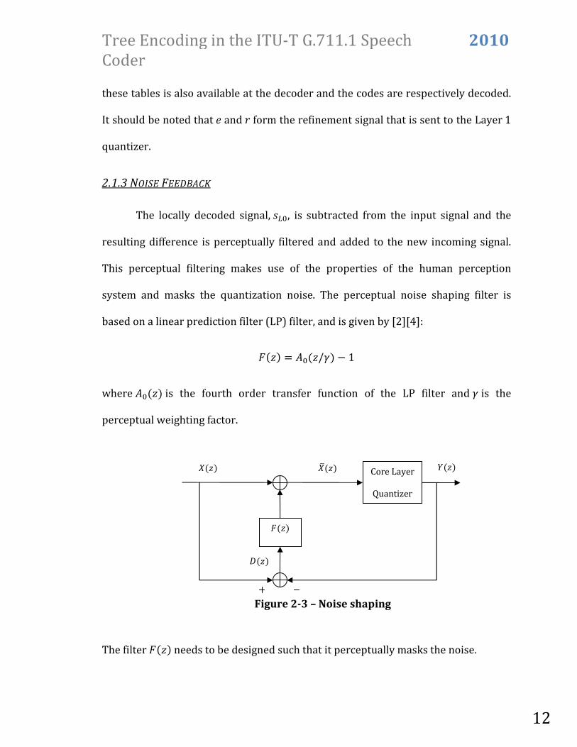
2.1.3 NOISE FEEDBACK

The locally decoded signal, ��, is subtracted from the input signal and the

resulting difference is perceptually filtered and added to the new incoming signal.

This perceptual filtering makes use of the properties of the human perception

system and masks the quantization noise. The perceptual noise shaping filter is

based on a linear prediction filter (LP) filter, and is given by [2][4]:

�(�) = ��(�/D) − 1

where ��(�) is the fourth order transfer function of the LP filter and D is the

perceptual weighting factor.

The filter �(�) needs to be designed such that it perceptually masks the noise.

�(�)

Core Layer

Quantizer

E(�)

F(�) FG(�) H(�)

Figure 2-3 – Noise shaping


Coder

2010

13

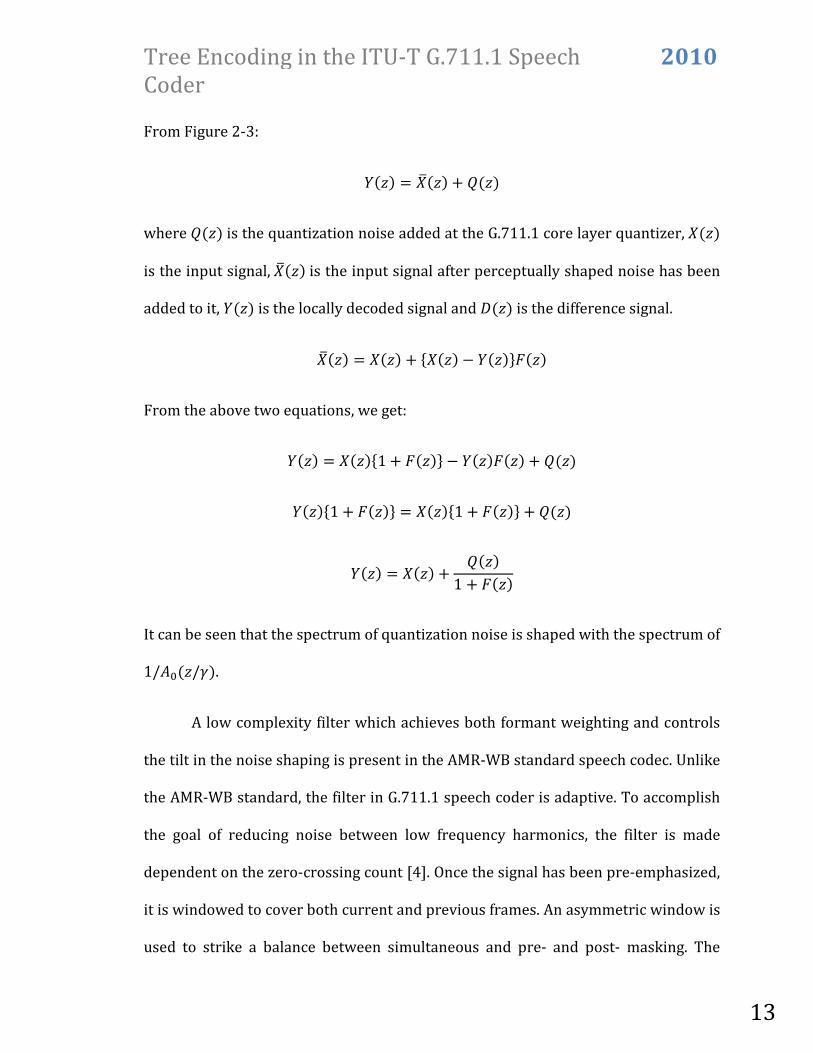
From Figure 2-3:

H(�) = FG(�) + �(�)

where �(�) is the quantization noise added at the G.711.1 core layer quantizer, F(�)

is the input signal, FG(�) is the input signal after perceptually shaped noise has been

added to it, H(�) is the locally decoded signal and E(�) is the difference signal.

FG(�) = F(�) + IF(�) − H(�)J�(�)

From the above two equations, we get:

H(�) = F(�)I1 + �(�)J − H(�)�(�) + �(�)

H(�)I1 + �(�)J = F(�)I1 + �(�)J + �(�)

H(�) = F(�) + �(�)1 + �(�)

It can be seen that the spectrum of quantization noise is shaped with the spectrum of

1/��(�/D).

A low complexity filter which achieves both formant weighting and controls

the tilt in the noise shaping is present in the AMR-WB standard speech codec. Unlike

the AMR-WB standard, the filter in G.711.1 speech coder is adaptive. To accomplish

the goal of reducing noise between low frequency harmonics, the filter is made

dependent on the zero-crossing count [4]. Once the signal has been pre-emphasized,

it is windowed to cover both current and previous frames. An asymmetric window is

used to strike a balance between simultaneous and pre- and post- masking. The


Coder

2010

14

Levinson-Durbin algorithm is then used to calculate the perceptual shaping filter

from the autocorrelation function of the resulting signal. Details of the

implementation can be found in [2]. The outcome LP analysis is a filter with the

transfer function:

��(�) = 1 + K�� + K/��/ + K9��9 + K>��>

After the weighing factor is included, it becomes:

��(�/D) = 1 +LDMKM��M>MN�

The noise feedback filter, hence, looks like:

�(�) = LDMKM��M>MN�

Usually a value of 0.92 is chosen for the weighting factor D. It is to be noted that this

filter is updated after each frame. At the encoder, noise shaping is only applied to

Layer 0. For Layer 1 the noise shaping filter is present at the decoder end. This is to

ensure that the shape of the quantization noise is the same when both layers are

used as that when only Layer 0 is in operation. As the noise shaping filter is based on

the past signals, there is no need to transmit it to the decoder, hence, bandwidth is

saved. It can be calculated at the decoder end from the past decoded signal. Details

of why the Layer 1 noise shaping filter should be at the decoder end are presented in

[4]. They are not listed here as this thesis is primarily concerned with Layer 0.


Coder

2010

15

There are two special cases where the noise feedback filter is attenuated. The

first case is when very low energy signals are received. The decision to attenuate the

filter in such a case based on the normalization factor, O, calculated as:

O = 30 − Alog/(3��(0))B where 3��(0) is the first autocorrelation coefficient of the pre-emphasized signal

from the calculation of the perceptual filter. Because of the limited dynamic range of

the G.711.1 quantizer, when a low level signal is received, the perceptual filter will

be unable to mask the noise [2]. In this case, when noise cannot be masked, it is best

to make it less annoying. A predefined filter is used.

When:

O ≥ 16

the filter becomes:

�(�) = L2�(M8P��Q)>MN� KM��M

This prevents the noise feedback filter from increasing the noise instead of masking

it. The second case occurs when signals with energy in higher frequency are

received, especially near 4kHz. The noise-shaping feedback might become unstable.

This would affect multiple incoming frames before it settles down [2]. Again the

filter is attenuated in this case. The first reflection coefficient, R�, computed in the

Levinson-Durbin algorithm is used to determine this condition.


Coder

2010

16

When:

R� S 0.9844

the weighting factor becomes:

D = 0.92T

where T is defined as:

T = 16 ∙ �1.047 � R��

The affect of noise shaping can be seen in Figure 2-4 [4]:


feedback (right) [4]

The noise-feedback filter masks the noise in the speech spectrum, as shown. In the

figure on the left hand side it can be seen that the noise on the low frequency end is

below the speech spectrum and, hence, inaudible. But in the higher frequency end

noise has more energy than the signal and can be heard. With noise shaping, this


Coder

2010

17

audible noise in the high frequency range is now masked beneath the speech

spectrum. Properties of the human perception system are utilized here. Even though

the overall noise energy is higher after filtering, it is inaudible due to masking. Once

the difference signal has been filtered, it is added to the new incoming signal.

(") = (") +LDMKM ∙ U(" − V)>MN�

The resulting signal is then quantized and the indices transmitted as the Layer 0

bitstream. The difference signal is based on the previous locally decoded signal. It

can also be viewed as filter memory.

2.1.4 DEAD-ZONE QUANTIZER

The second major addition is the dead-zone quantizer. Like the attenuation in

the noise feedback filter, it targets very low energy signals. The lowest quantization

steps in a �-law quantizer are 0 and ±7. Very low level signals, like those of faint

ambient noise, can often find themselves high enough to be quantized to the ±7

level. This increases the noise in the coded signal. In this case the output of the

quantizer is brought down to the zero level. This is done to further perceptually

improve the quality of the signal. The dead-zone quantizer is triggered when:

O ≥ 16

and

−7 ≤ (") ≤ +7


Coder

2010

18

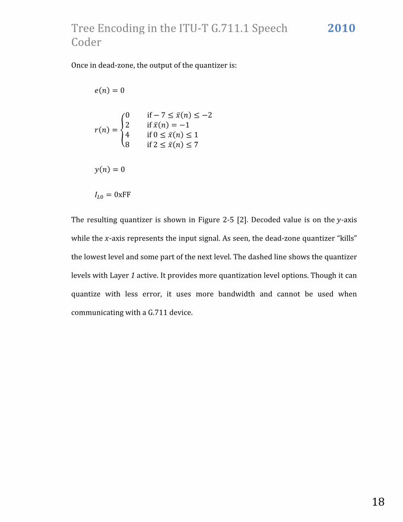
Once in dead-zone, the output of the quantizer is:

*(") = 0

3(") = Y0if − 7 ≤ (") ≤ −22if (") = −14if0 ≤ (") ≤ 18if2 ≤ (") ≤ 7 :(") = 0

)�� = 0xFF

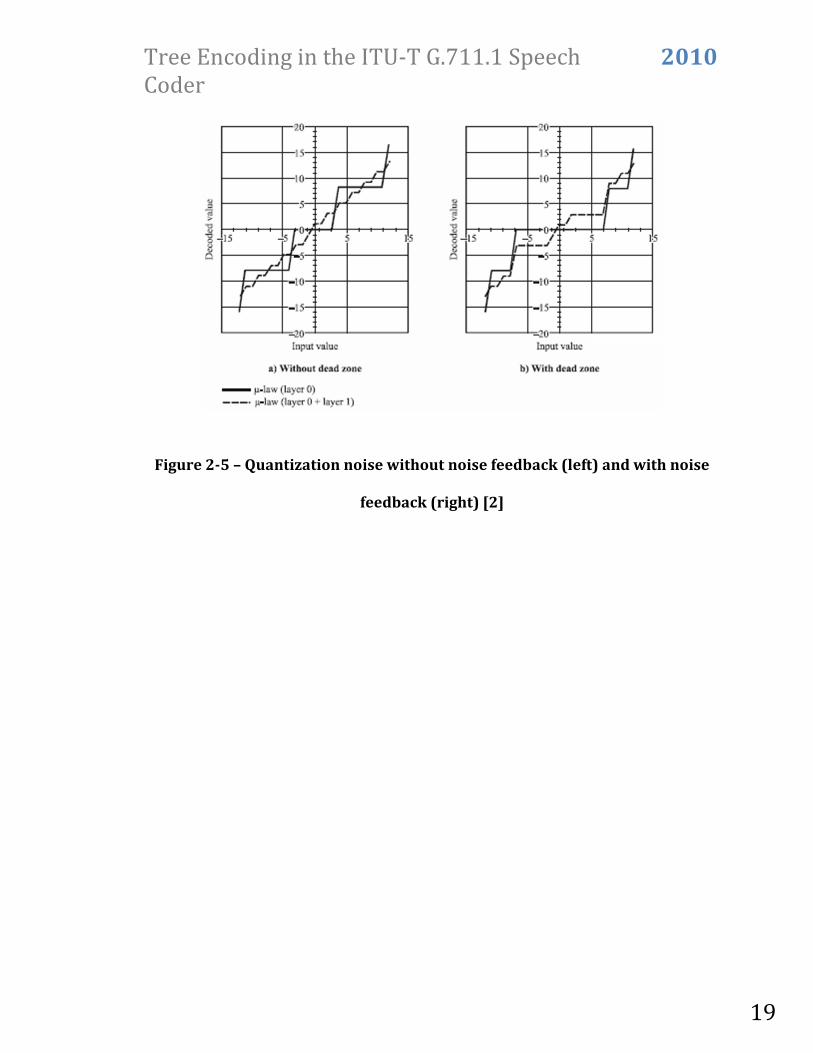
The resulting quantizer is shown in Figure 2-5 [2]. Decoded value is on the :-axis

while the -axis represents the input signal. As seen, the dead-zone quantizer “kills”

the lowest level and some part of the next level. The dashed line shows the quantizer

levels with Layer 1 active. It provides more quantization level options. Though it can

quantize with less error, it uses more bandwidth and cannot be used when

communicating with a G.711 device.


Coder

2010

19


feedback (right) [2]


Coder

2010

20

Chapter 3 CELP AND VECTOR QUANTIZATION IN

ADPCM

G.711.1, being a log companded PCM coder with modifications, falls in the

category of waveform coding. Another similar coder working at a lower bit rate is

the DPCM coder. Instead of quantizing the input signal, the DPCM coder takes the

difference from a prediction based on the past values and quantizes and codes that.

With this the noise ends up being shaped by the synthesis filter. This is solved in

ADPCM where feedback is utilized to counteract this noise shaping. In this chapter a

basic overview of DPCM and ADPCM coder is provided. Then we go on to discuss

CELP coding, a hybrid coder making use of linear prediction and quantizing the

residue. Instead of sample-by-sample quantization like the other two coders, CELP

employs vector quantization. In the last subsection the structure of the ADPCM is

rearranged into a noise feedback version and vector quantization is introduced. It

can be seen that such a setting is similar to that of CELP [5].


Coder

2010

21

3.1 DPCM

A DPCM system involves a prediction filter and a quantizer at the coder end

and an analysis filter at the decoder end. A high level DPCM block diagram is shown

in Figure 3-1.

Based on the past values of the input signal, the prediction filter Z(�) creates

an approximation of ("). Usually it is a multi-coefficient filter based on the input

signal. It can be computed by solving for the linear predictor coefficients which

minimize the mean square error. The difference signal U(") is then quantized and

passed on to the receiver. In an actual scenario indices of the quantization are

transmitted and the reconstructed takes place at the decoder end. For simplicity this

step is skipped and the quantizer is shown to transmit the reconstructed signal.

Analyzing the encoder side it can be seen that:

�(�) = 1 − Z(�)

where �(�) is the analysis filter. The inverse of this, the synthesis filter, is found at

the decoder end. Analyzing the decoder:

Z(�)

(") Q

U(")

[(")

U(")

Z(�)

U(") \(")

Figure 3-1 – DPCM Coding; encoder on the left, decoder on the right


Coder

2010

22

F](�) = 1�(�) E(�)

F](�) = F(�)�(�) − �(�)�(�)

F](�) = F(�) − �(�)�(�)

where �(�) is the quantization noise given by:

�(�) = E(�) − E(�)

This shaping of noise by the synthesis filter is undesirable. The solution of this

comes in the form of ADPCM.

3.2 ADPCM

A feedback structure is employed to adapt to the input signal. The decoder is

the same as before, but the encoder is modified, as shown in Figure 3-2.

Q

U(") U(")

Z(�)

(")

\(") [(")

Figure 3-2 – ADPCM encoder block diagram


Coder

2010

23

The encoder now has a locally decoded signal. Looking at the different

relationships between the signals, it can be seen that:

F](�) = E(�) + F_(�)

F](�) = E(�) − �(�) + F_(�) F](�) = F(�) − F_(�) − �(�) + F_(�)

F](�) = F(�) − �(�)

By the addition of the feedback, the noise shaping by the synthesis filter has been

removed. The coding process only adds quantization noise, which is white in nature.

3.3 CELP

Unlike ADPCM, CELP employs a vector quantizer codebook. As stated earlier,

CELP is an analysis-by-synthesis coder. Entries from the codebook are used to

synthesize the output at the encoder and compared with the input signal. The entry

that gives the best match is selected. The same synthesis filter is used here as in

ADPCM. The quantization error is weighted and filtered to give a better perceptual

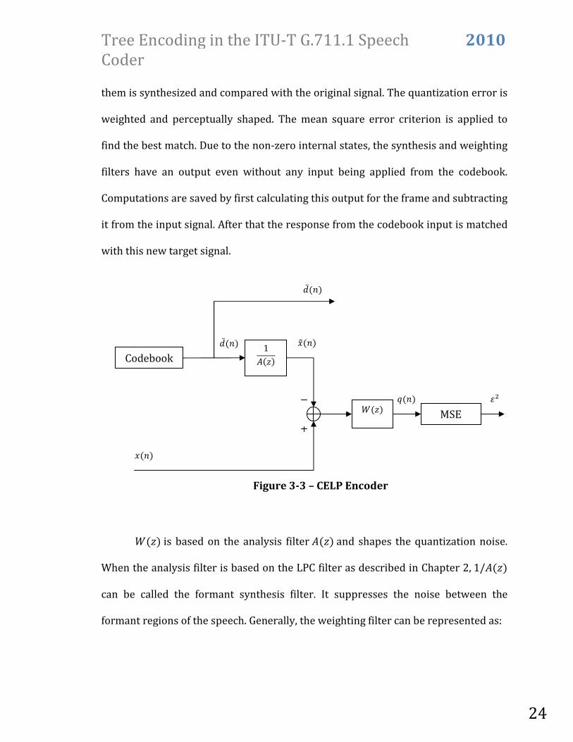
result. A higher level block diagram of a CELP encoder is shown in Figure 3-3. The

decoder is again the same.

`(�) is the weighing filter. The codebook keeps a set of possible quantization

values for the difference signals for an entire frame. A reconstructed signal from


Coder

2010

24

them is synthesized and compared with the original signal. The quantization error is

weighted and perceptually shaped. The mean square error criterion is applied to

find the best match. Due to the non-zero internal states, the synthesis and weighting

filters have an output even without any input being applied from the codebook.

Computations are saved by first calculating this output for the frame and subtracting

it from the input signal. After that the response from the codebook input is matched

with this new target signal.

`(�) is based on the analysis filter �(�) and shapes the quantization noise.

When the analysis filter is based on the LPC filter as described in Chapter 2, 1/�(�)

can be called the formant synthesis filter. It suppresses the noise between the

formant regions of the speech. Generally, the weighting filter can be represented as:

Codebook 1�(�)

`(�) MSE

(")

U(")

U(") \(")

a(") b/

Figure 3-3 – CELP Encoder


Coder

2010

25

`(�) = �(D��)�(D/�)

where D� and D/ are parameters used to control the shape of the filter.

3.4 VECTOR QUANTIZATION IN ADPCM

A CELP coder essentially takes a predicted value, takes the difference from

the original input, quantizes the difference, perceptually shapes the quantization

noise and makes the decision based on mean square error criterion. It uses the same

synthesis filter as ADPCM. ADPCM itself does some noise shaping; it reshaped the

quantization noise in DPCM back to white. If the ADPCM structure is further

tweaked, the noise shaping property will be further clear. An equivalent structure of

the encoder to that of Figure 3-2 is shown in Figure 3-4.

The presence of Z(�) in the noise feedback path cancels the noise shaping

effect of DPCM. If we replace it by a general noise feedback filter, c(�), the noise can

be shaped as desired.

(") Q

U(")

[(")

U(")

Z(�)

Z(�) a(")

Figure 3-4 – Rearranged ADPCM encoder structure to show noise feedback


Coder

2010

26

F](�) = F(�) − 1 − Z(�)1 − c(�)�(�)

It would be advantageous if this is made use of and the noise is masked perceptually,

a property present in CELP coding. It can be seen that the only major difference left

between ADPCM and CELP is the mechanism of quantizing the samples; one is

sample-by-sample while the other is vector quantization. Replacing the sample-by-

sample quantizer in ADPCM by a codebook based VQ, the new structure of ADPCM

looks like Figure 3-5.

The encoder can now quantize multiple samples at a time. The codebook

consists of all possible quantizer outputs. These outputs are predetermined

approximations of the difference signal under the quantization law being

implemented. The outputs are compared with U("). The quantization error, a("), is

fed into the noise feedback loop. The codebook vector with the least error as

calculated by the mean square error block (MSE) is chosen and transmitted. Further

(")

U(")

[(")

U(")

Z(�) c(�)

a(")

Codebook

MSE

b/

Figure 3-5 – VQ in ADPCM encoder with noise feedback


Coder

2010

27

modifying the structure, we get the arrangements as shown in Figure 3-6 and Figure

3-7.

Form 1 is a rearrangement of structure in Figure 3-5. In form 2 the analysis

and noise feedback filters are merged. It can be seen that this is similar to the CELP

encoder in Figure 3-3. ADPCM, a waveform coder with a scalar quantization (SQ),

has been modified to have noise feedback and vector quantization, just like CELP, a

hybrid coder. A similar modification can be performed with the G.711.1 core layer.

The benefit is that noise feedback is already present in the new standard; all that

needs doing is replacing the quantizer with a similar codebook based vector

quantizer which follows the �-law so that it is compatible with other G.711 devices.

It should be noted that these modifications have been done at the encoder side and

nothing needs to be done with the decoder as it has remained the same throughout.

This goes along with the aim to keep the bitstream G.711 compatible.


Coder

2010

28

Codebook

�(�)1 − c(�) MSE

U(")

a(")

(")

1�(�) U(")

\(")

Codebook

11 − c(�) MSE

U(")

a(") b/

U(")

(") �(�)

Figure 3-6 – VQ in ADPCM encoder with noise feedback – form 1

Figure 3-7 – VQ in ADPCM encoder with noise feedback – form 2


Coder

2010

29

Chapter 4 DELAYED DECISION CODING

A vector quantizer takes a batch of input samples and quantizer them at the

same time. The aim is the minimization of propagating effect of pervious decision

over the whole batch. This approach is better than sample-by-sample quantization

as it has a better view of the incoming samples. It is slightly rigid in the sense that it

can only make the best possible decision based on the current batch of input

samples and is blind to the future inputs and the effects the decision now would

have on them. Also when noise feedback is included the effect of pervious decision

can propagate further, even increase, due to filter memory. As mentioned earlier the

CELP filters already have a zero input response. This is beyond the control of the

quantizer as its scope is limited to the current set of input samples. In a CELP coder

an entire 5ms frame (40 samples) is processed at the same time by the vector

quantizer. Due to the large set of samples the effect of this propagating error is not

that profound. A �-law quantizer already has 256 quantization levels. To replace it

by a vector quantizer, multiple samples have to be quantized at the same time. The

vector quantizer codebook tremendously increases in size even when one more

sample is added (65,536 codebook entries for two samples). To keep the complexity


Coder

2010

30

low, only two samples are quantized at the same time. Hence, the propagation of

error due to noise feedback and filter memory will have a much greater effect. To

counter that delayed decision coding is suggested. A coding technique which waits

for further samples to arrive, evaluate the effect of different decisions on these

future samples and then makes the best possible decision. If a vector quantizer can

be viewed as jumping from frame to frame, delayed decision coding can be viewed

as sliding across the frames.

4.1 TREE ENCODING

One such delayed decision coding method is tree encoding. A tree is

populated with different possible decisions when new samples are received.

Cumulative errors over the branches are taken into consideration. Once a decision

has been made, the tree is pruned to keep the complexity under control and to

remove the branches which will not be further expanded. Examples of tree encoding

can be found in [3], [6] and [7].

4.1.1 SINGLE PATH TREE ENCODING

Single path tree encoding is much simpler than multi-path tree encoding. It is

being mentioned over here to describe some tree encoding terms which are

common in both. Three important terms are associated with tree encoding:

• Nodes

• Branches

• Leaves


Coder

2010

31

A node is a time instant which has a quantizer output associated to it. For a single

path tree encoder a tree is only left with one node once a decision has been made.

The quantizer output associated with it is the best possible approximation of the

input samples based on the error criterion. Whenever new samples are received and

decision has to be made, the tree is expanded from this node. For case of a two

sample �-law vector quantizer, 65,536 branches stem from it. At the end of each

branch is a leaf. The leaf holds the possible quantizer values which could be selected

for this time instance. Once the best possible match has been selected, the selected

leaf becomes the node for the next round and the rest of the leaves are discarded.

Therefore, only one path is kept. The tree is continuously populated and pruned, and

in the end one single path is left which defines the code. There is no delay in the

coding of the samples. The code can be transmitted as soon as the decision is made.

This type of coding can be seen in CELP. If a vector quantizer is replaced by a scalar

version, it can also be seen in PCM encoders.


Coder

2010

32

4.1.2 MULTI-PATH TREE ENCODING: THE (�, �)—ALGORITHM

In a single path tree encoder only one node is available each time the tree is

branched out. There is no delay in making the decision as the code can be

transmitted almost instantaneously. If an artificial delay is added and the decision is

reserved till its effect on further decisions can be evaluated, multi-path tree

encoding is realized. The tree is branched from multiple nodes and, therefore, many

more leaves are available to choose from. The (�, �)—Algorithm is used to

implement the multi-path tree encoder. This algorithm is similar to the one

implemented in [3].

0

1

2d − 1

Node

V − 1 V V + 1 V + 2 V + 3 V − 2

Branch

Leaf

Figure 4-1 – Single path tree encoding


Coder

2010

33

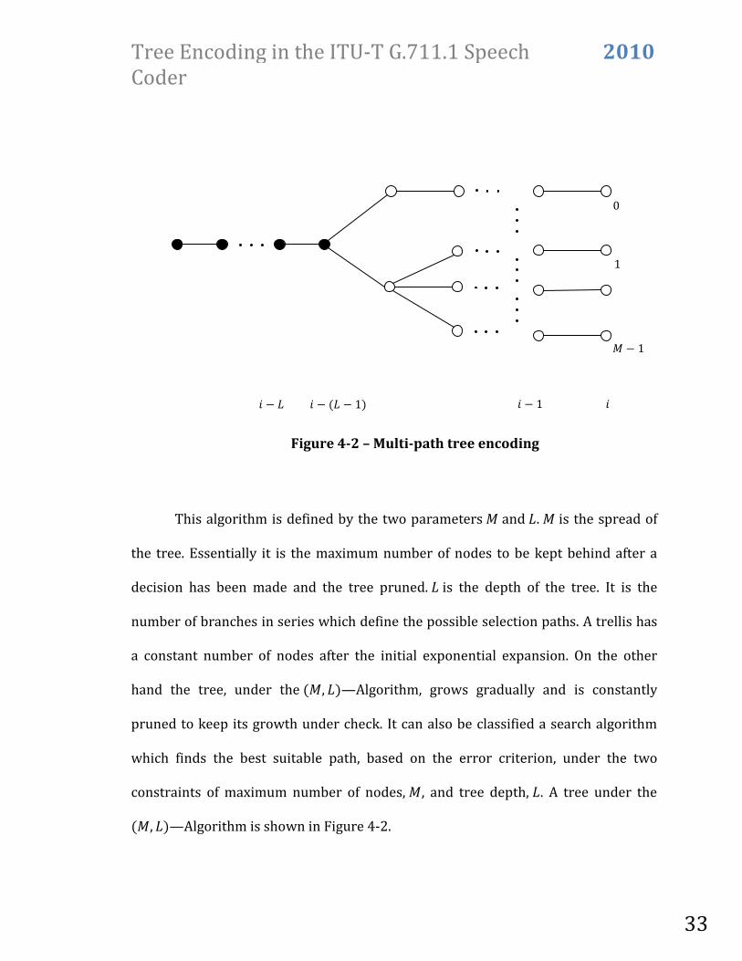
This algorithm is defined by the two parameters � and �. � is the spread of

the tree. Essentially it is the maximum number of nodes to be kept behind after a

decision has been made and the tree pruned. � is the depth of the tree. It is the

number of branches in series which define the possible selection paths. A trellis has

a constant number of nodes after the initial exponential expansion. On the other

hand the tree, under the (�, �)—Algorithm, grows gradually and is constantly

pruned to keep its growth under check. It can also be classified a search algorithm

which finds the best suitable path, based on the error criterion, under the two

constraints of maximum number of nodes, �, and tree depth, �. A tree under the

(�, �)—Algorithm is shown in Figure 4-2.

0

1

� − 1

V V − 1 V − (� − 1) V − �

Figure 4-2 – Multi-path tree encoding


Coder

2010

34

After the Vef input block has been processed, a maximum of � nodes are kept.

There is an equal number of paths present as each node signifies one path. If traced

backwards it can be seen that all these paths converge back to a node at time

V − (� − 1). Hence, when the Vef input block has been processed, the decision has

been made on the 0V − (� − 1)1ef node. The code for that block is transmitted.

Therefore, an artificial delay of � − 1 is created.

At the next instance when (V + 1)ge block is input, each of the � nodes is

populated with 2d number of nodes. For a �-law vector quantizer working on two

samples the code book has 65,536 entires. Hence, � is 16. At the end of each branch

is a leaf, which has a possible quantizer value associated with it. As compared to the

single path tree encoder, � times more output choices are available. The nodes are

populated with the same set of codebook entries, but because each branch originates

from a different node, which has a different quantizer value associated with it, all the

new leaves are different and unique. Each path has its own error associated with it,

and the filter states on each path are different as well. To ensure this uniqueness it

has to be made sure that when the tree is pruned after a decision making instance,

each of the � paths that are left behind is different. Some tree encoding

implementations might require that the branch numbers be transmitted [3], but in

this case the bitstream needs to be G.711.1 compliant. Hence, the indexes of the

quantizer decisions are sent. Therefore, the fact that there are different branches

which have the same branch number because all the nodes have been expanded

from the same codebook does not interfere with the coding process.


Coder

2010

35

Once the nodes have been populated, the leaf with the best quantization

output associated with it according to the cumulative error criterion, to be described

later, is chosen. Once this selection, at time V + 1, is done, the branch is traced back

to the time V − (� − 2) and the node which leads to this selected leaf at time V + 1 is

chosen as the best code for the 0V − (� − 2)1ef input block. The codebook index for

the quantization value associated with this node is, hence, transmitted. After this,

the tree is pruned and a maximum of � paths are selected and kept behind. The path

linking the leaf which was selected to have the best quantization output associated

with it at the time V + 1 and the optimal node for the time instance V − (� − 2) is

always included. It has to be ensured that all of the paths have to converge to the

newly selected optimal node for the time instance V − (� − 2). This is to maintain the

continuity of the optimal path. The � paths which are kept behind are based on the

cumulative error. This encoding process continues as further blocks are input.

There is an upper bound on the number of branches that can be kept behind.

The maximum number of nodes in a tree, for a depth of � are 2d(��). Therefore,

� ≤ 2d(��) There are two special cases of multi-path tree encoding. The first one is when � = 1.

In this case � = 1 as well and single path tree encoding is realized. When � is at its

upper bound, all possible paths are considered. Even though this is the optimal

approach, it increases the complexity drastically. Hence, the value of � is kept less

than 2d(��). Even though this is not optimal, enough paths are considered to


Coder

2010

36

provide a near optimal solution while keeping the complexity low. The other special

case is when � = 1. In this case only one node is kept back after the decision has

been made. There is no point in keeping � larger than 1 because there is only one

single path. Increasing the tree depth would only add delays without any benefits.

Hence, when either � or � is 1, the other is as well.

4.2 CUMULATIVE ERROR

The error measure decides how the tree is populated and in turn pruned.

Hence, it plays a vital role in tree encoding. The benefit of a tree encoder is that it

looks at future values and sees how a decision made now will have an effect on them.

To make use of this property it is only wise to use an error measure which looks at

long term distortions. Therefore, the cumulative error over the whole path is chosen

to be the error measure. To be more specific, the cumulative sum of the mean square

error of all nodes in the path is considered. At the time instant V + 1 decision is made

for the code for the input block at time instant V − (� − 2). It is chosen such that:

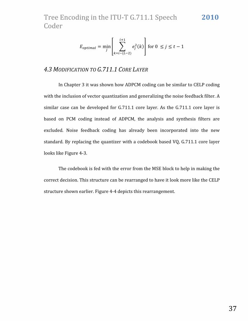
hije = minm nL*m/(R)M8�oN� p for0 ≤ r ≤ s − 1

where hije is the cumulative error of the chosen path, *m/(R) is the mean square

error at a node at the ref branch at time instance R and s is the number of paths

available at time V + 1. As all the paths originate from the already chosen node at

time V − (� − 1), the cumulative error till that point is common to all paths. This can

eliminated and the equation for the optimal cumulative error is modified to:


Coder

2010

37

hijeMdtu = minm n L *m/(R)M8�oNM�(��/) p for0 ≤ r ≤ s − 1

4.3 MODIFICATION TO G.711.1 CORE LAYER

In Chapter 3 it was shown how ADPCM coding can be similar to CELP coding

with the inclusion of vector quantization and generalizing the noise feedback filter. A

similar case can be developed for G.711.1 core layer. As the G.711.1 core layer is

based on PCM coding instead of ADPCM, the analysis and synthesis filters are

excluded. Noise feedback coding has already been incorporated into the new

standard. By replacing the quantizer with a codebook based VQ, G.711.1 core layer

looks like Figure 4-3.

The codebook is fed with the error from the MSE block to help in making the

correct decision. This structure can be rearranged to have it look more like the CELP

structure shown earlier. Figure 4-4 depicts this rearrangement.


Coder

2010

38

Again it is seen that it has a similar structure, only the analysis and synthesis

filters are missing as G.711.1 works on the original input signal without making any

prediction. G.711.1 already has the weighting filter built into it as the noise feedback

Codebook

11 − c(�) MSE

a(") b/

(")

:(")

:(")

(") a(")

Codebook

MSE

b/

(")

:(")

c(�)

Figure 4-3 – G.711.1 core layer with codebook VQ

Figure 4-4 – G.711.1 core layer with codebook VQ - rearranged


Coder

2010

39

filter. It is based on the human perception system and shapes the noise accordingly.

Therefore, there is no need to modify that. Tree encoding was chosen because a

vector quantizer does not care about the effect its decisions have on the future input

values due to the filter memories. In a �-law codebook vector quantizer only a few

samples can be quantized at the same time due to complexity concerns as an

increase of one more in the block size increases the codebook size 256 times its

previous size. Therefore, the block size has to be kept small. With a smaller block

size there are more decision instances, hence, there are more instances when the

quantizer is ignorant of the effect its decision would have on the incoming samples.

To overcome this short coming, delayed decision coding, tree encoding to be more

precise, has been introduced. Once implemented the G.711. core layer looks like the

tree in Figure 4-2 with each new leaf having a modified G.711.1 core layer encoder

like that of Figure 4-3 (or Figure 4-4 as they are both the same) on it, with the

difference that each leaf only has one codebook entry associated with it and the

error is not fed to the codebook. The (�, �)—Algorithm is then employed.


Coder

2010

40

Chapter 5 COMPUTER SIMULATION

Until now the theories behind the system have been discussed, and the structure

of the modification to be performed. In this chapter the computer simulation of the

encoder will be explained. The simulation was performed on a Dell Studio Desktop, a

Quad-core Core 2 Quad 2.8 GHz, 8GB RAM computer running Windows Vista 64-bit

edition. The programming has been done in MatLab. In the initial sub-sections the

sub optimization of the codebook to reduce the complexity of the encoder, the

initialization of the system and the simulation inputs are discussed. Later on a

performance evaluation method, perceptual evaluation of speech quality (PESQ) [9],

[10], is described and the simulation results provided. The performance of both

vector quantized G.711.1 core layer and tree encoded G.711.1 core layer is compared

with that of the G.711.1 core layer as in the ITU-T standard. Later on performance of

the tree encoder as � and � are varied is provided for further insight.

5.1 SUB OPTIMAL APPROACH TO REDUCE COMPLEXITY

Complexity is a very important parameter of a speech encoder. It is directly

related to the size of the codebook. A �-law encoder has 256 levels, for each input


Coder

2010

41

sample. Hence, for each additional sample in the input block, the codebook size

increases 256 times. To keep the codebook from having an enormous size the size of

the input block has been restricted to 2. This means the codebook has 65,536

entries. This is still a very large size as compared to a typical CELP codebook (1024

entries). To cut down on it, a sub optimal approach is proposed. For each input block

instead of looking at the entire codebook to find the optimal match, the search is

performed in the local neighbourhood of the input samples. For this purpose the

input block is first quantized by a scalar �-law quantizer, without the addition of

noise feedback. This is done by using tables to cut down on the processing time.

Once quantized, the neighbouring quantization intervals are chosen as the sub

optimized codebook for the population of the tree. The neighbourhood need not be

large as a �-law quantizer has pretty large quantization intervals. The neighbour

hood is chosen to be ±2 samples of each input sample. That makes 5 choices for each

input sample, including itself. With a block size of 2 the sub optimized codebook has

a size of 25.

In the G.711.1 core layer there are two major operations. There is one

quantization operation and one filtering operation. With a vector quantizer there is

one quantization operation but the number of filtering operations is increased to the

size of the sub optimized codebook, which is 25, as each entry has to be filtered. In a

tree encoder there is still only one quantization operation but the number of

filtering operations is now �-times the size of the sub optimized codebook, because

all the � paths that have been kept behind have to be branched. It should also be


Coder

2010

42

noted that even though the complexity of each filtering operation in a vector

quantizer and tree encoder is twice that of G.711.1 core layer, because 2 samples are

being coded, the per sample complexity of each filtering operation is still the same.

The filtering operation is the main resource consuming activity. In G.711.1 each

filtering operation, per sample, has 4 multiplication operations and 3 addition

operations. The vector quantizer has 25 times that many. For a tree encoder that

figure is further increased by �-times. Also in vector quantization and tree encoding

after each filtering operation mean square error is calculated. Each mean square

error calculation for two samples requires 2 multiplication operations and 3

addition operations.

For a typical value of � = 3, the increase in complexity for tree encoding is

substantial. G.711.1 has considerable processing power which it requires for the

lower-band enhancement layer and the higher-band layer. When working at 64 kbps

only the core layer is present. All the processing power available for the other two

layers does not get utilized. As tree encoding only works with the core layer, in this

certain scenario it can be turned on to make use of the already present processing

power, which would otherwise remain unused.


Coder

2010

43

Encoder Multiplication operations Addition operations

G.711.1 Core Layer, 64 kbps 4 3

G.711.1 Core Layer with VQ, 64 kbps

25 × 4 + 25 × 1 25 × 3 + 25 × 3/2

G.711.1 Core Layer with Tree

Encoding, 64 kbps

� × (25 × 4 + 25 × 1) � × (25 × 3 + 25 × 32)

Table 5-1 – Multiplication and addition operations per sample of different

G.711.1 encoders


Coder

2010

44

5.2 INITIALIZATION OF THE SYSTEM

The initial state of the system is very important and affects the performance.

A good many variables define this initial state. These include filter memories,

feedback filter coefficients and initial multi-path tree.

The filter memories and feedback filter coefficients are all set to zero for ease. In

the simulated implementation the multi-path tree is represented by a three

dimensional tree. The rows represent different nodes at a certain time instance

while the columns hold different variables associated with that node. The third

dimension represents the different time instances. The variables associated with

each node are:

• Quantized value of first sample

• Quantized value of second sample

• Cumulative error till that node

• Row number of previous node in the path

• Noise feedback filter memory

Each node needs to know its predecessor so that the optimal path can be traced

back. Each decision has its own effect on the future values by altering the noise

feedback filter memory. Therefore, it is vital to keep track of it. All of these variables

are initialized to zero. This means at the initialization the tree is essentially a single

path and branches out to � nodes for the last decision making instance.


Coder

2010

45

5.3 SIMULATION INPUTS

As input to the system four speech sentences were used. They were recited by

two different speakers, one male and one female. The sentences are:

• The empty flask stood on the tin tray.

• A speedy man can beat this track mark.

• It is easy to tell the depth of a well.

• These days a chicken leg is a rare dish.

Each speaker recited two consecutive sentences. The male speaker recited the

first two sentences while the female speaker recited the last two. All of these

samples are combined into one input signal, sampled at 8Rw�.

5.4 PERFORMANCE

Performance results are listed in this sub-section. The performance has been

evaluated using the performance evaluation method PESQ. A brief explanation of

this is method is provided in the following sub-section.

5.4.1 PERCEPTUAL EVALUATION OF SPEECH QUALITY

The standard ITU-T P.862 [10] is an objective method to assess the end-to-

end speech quality of a narrow band speech coder. To evaluate the coder, the

original input signal to the encoder and the output from the decoder is compared.

The result is a prediction of the perceived quality. The amplitude of both the signals

is adjusted and brought to a standard level. The degraded signal (output from the


Coder

2010

46

decoder) is then time aligned with the original signal. Delays during both silence

periods and speech periods can be handled by the algorithm. After that both the

original signal and the time aligned degraded signal are transformed into an internal

representation. The transformation is such that to match the auditory system of the

humans. The transformation has different steps which include Bark spectrum

calculation, frequency equalization, equalization of gain variation and loudness

mapping. Once both the signals have been transformed by this perceptual model, the

difference is passed through a cognitive model. The output is similar to that of MOS

scores. The output range of the score is −0.5 to 4.5. The output score is based on the

two parameters that are calculated by the cognitive model [9], [10].

Zhx�xyz3* = 4.5 − Ug − 0.0309Utg where Ug is the symmetric disturbance and Utg is the asymmetric disturbance as

calculated by the cognitive model.

5.4.2 COMPARISON WITH G.711.1

According to the theory, both the quantizer modified with codebook based

VQ and delayed decision coding implemented by the (�, �)—algorithm should

perform better than the original G.711.1 core layer quantizer. To evaluate this

comparison has been made at two different signal power levels. In the first scenario

the signal is fed in without any attenuation. The quantizers are not saturated and use

as many of the quantization levels available as possible. In the second scenario the

power of the signal is attenuated by −40U{ to force the quantizer to use fewer


Coder

2010

47

quantization levels. This is done to evaluate the performance of the encoders at

lower xc| and increased quantization noise. The PESQ scores for the three cases

under the two scenarios are listed in table 5-2. Scores for G.711.1 core layer with

lower-band enhancement layer switched on are provided as well.

Encoder Signal without attenuation Signal at −40U{ attenuation

G.711.1 Core Layer, 64 kbps 4.252 2.263

G.711.1 Core Layer with VQ, 64 kbps 4.306 2.616

G.711.1 Core Layer with Tree

Encoding (� = 3, � = 3), 64

kbps

4.314 2.625

G.711.1 Core Layer with

Lower-band Enhancement

Layer, 80 kbps

4.421 3.310

Table 5-2 – Comparison of different G.711.1 encoders using PESQ

At 64 kbps, as expected, the tree encoder provides the best result, with the

vector quantizer being better than the G.711.1 core layer. This holds true for both

the signals, with and without attenuation. With the luxury of coding more than one

sample at the same time, both the VQ and the tree encoder are able to make better

decisions. The tree encoder is further able to improve by looking at future values.

With the availability of more data rate ( 80 kbps), the lower-band

enhancement layer can be switched on. As seen in Figure 2-5, the lower-band

enhancement layer increases the number of quantization levels available. The finer

quantization allows it to produce results with less quantization noise. This provides


Coder

2010

48

an increase in performance (Table 5-2), but at the cost of increased data rate. This

performance increase is more noticeable in the case of the attenuated signal. In this

scenario, when a reduced number of quantization levels are used, the enhancement

layer reaps the full benefit of its increased quantization levels. Tree encoding does

take a step towards reaching this performance level, but at the original data rate

requirement of 64 kbps. Another advantage of tree encoding is that while the lower-

band enhancement layer is not compatible with the legacy G.711 decoders, G.711.1

core layer with tree encoding is. Hence, increase in performance at the same data

rate without the replacement of the already installed G.711 decoders can be

achieved.

In a subjective test, for the signal without attenuation, at 64 kbps, the

difference between the signals encoded with the different encoders is barely

noticeable. Though, it can be said with certainty that the subjective quality of the

signals encoded with the modified encoders is not less than that of the signal

encoded with the original G.711.1 core layer encoder. For the attenuated signal, the

modified encoders provide a better result. The speech is less broken, especially in

the case of the tree encoder, as it has access to the future values while making the

decision. As was the case with the PESQ scores, with the addition of the lower-band

enhancement layer, at 80 kbps, the increase in subjective quality is even more still.

Even though tree encoding does not reach this quality, it does have two advantages

over the use of the lower-band enhancement layer. The increase in quality due to


Coder

2010

49

tree encoding can be availed without any increase in data rate and with the already

installed G.711 decoders.

5.4.3 PERFORMANCE AS A FUNCTION OF �

As stated earlier, � defines the spread of the tree. More precisely it is the

maximum number of nodes kept at the end of each decision making instance where

the optimal output decision is made for a delayed input block. It was shown that � is

upper bounded, and depends on the size of the codebook and on the depth of the

tree, or the artificial delay. Increase in �, within this upper bound, means more

nodes are kept back after each decision making instance. Hence, more leaves are

available when a new input signal is received, depending on the size of the sub

optimal codebook.

The performance of the system as a function of � for a signal attenuation of

−40U{ is plotted in Figure 5-1. Performance of G.711.1 core layer is provided for

reference. The value of � is kept constant at 6 except for the case when � = 1. In

that case, � is equal to 1 as well, as described in an earlier section. The performance

increases as the tree encoder is turned on, but it saturates very quickly. Subjectively

there is not much difference between the different tree encoded signals as such a

small difference cannot be detected.


Coder

2010

50

Figure 5-1 – PESQ score of tree encoding as a function of M, with L=6 at -40 dB.

For the first point M=1 and L=1. The performance of G.711.1 core layer is

provided for comparison.

In the case of a �-law quantizer, where the quantizer has a large range and

large quantization intervals, there will be a lot of codewords which do not give

satisfactory error results when used to approximate the input block. With a smaller

� these tend to get eliminated very quickly. Only the good approximations are kept.

The benefit can be seen by the sudden increase in the performance of the encoder as

compared to the original G.711.1 core layer encoder.

The saturation of the performance is because when � increases many of the

codewords with bad performance are kept. The tree encoder keeps on ignoring

them because they do not give good results. The cumulative errors on these paths

2.2

2.25

2.3

2.35

2.4

2.45

2.5

2.55

2.6

2.65

0 2 4 6 8 10 12 14 16

PE

SQ

Sco

re

M

Tree encoder

G.711.1


Coder

2010

51

keep on increasing. Even certain good approximations down the path cannot reduce

the accumulated sum. Even though these are kept due to a large value of � they are

not chosen because there are other options available with better cumulative errors.

Hence, the optimal path is more or less the same. Therefore, high performance can

be achieved without taking � to its upper bound. Once saturated, any increase in �

only results in increase of encoder complexity.

5.4.4 PERFORMANCE AS A FUNCTION OF �

The parameter � defines the depth of the tree. More specifically it defines

how many blocks of input data would be looked at before making the decision.

Hence, it also defines the artificial delay that is created. The purpose of � is that the

quantization error be averaged out over a larger number of samples. Once � S 1,

multi-path tree encoding is realized. It also defines the upper bound on �, hence, the

spread of the tree. This bound increases drastically with an increasing � and, hence,

soon loses its significance.


Coder

2010

52

Figure 5-2 – PESQ score of tree encoding as a function of L, with M=6 at -40 dB.

For the first point L=1 and M=1. The performance of G.711.1 core layer is

provided for comparison.

Figure 5-2 shows the perceptual performance of the tree encoder as a

function of �, at a signal attenuation of −40U{. The PESQ score of G.711.1 core layer

is provided as reference. For the case of � = 1, � is also equal to unity. As was the

case with � it is seen that there is a sudden increase in performance as the tree

encoder is kicked in and then the performance saturates out. In the beginning the

benefit is because the encoder can look at more values and it can take into

consideration the effect on future values. After a limit the quantization error cannot

be averaged out further more. Also, the noise feedback filter has a filter memory of 4

and the block size is 2. With a small � the effect on future samples due to filter

memory is taken care of. Once � gets large the benefit tends to decrease because the

2.2

2.25

2.3

2.35

2.4

2.45

2.5

2.55

2.6

2.65

0 2 4 6 8 10 12 14 16 18 20

PE

SQ

Sco

re

L

Tree encoder

G.711.1


Coder

2010

53

major effect of filter memory is only short term. Also, the large quantization

intervals of �-law quantizer do not provide enough room in terms of selection of

different codewords. A further increase in the tree depth only results in an increase

of encoder complexity without any performance increase.


Coder

2010

54

Chapter 6 CONCLUSION

The use of delayed decision coding in ITU-T G.711.1 wideband extension

standard has been studied in this thesis. The thesis started off by describing the core

layer of the standard in Chapter 2. In Chapter 3 the similarities between vector

quantized ADPCM and CELP coding were discussed. Similar structures for both were

derived and a similar modification of inclusion of vector quantizer in G.711.1 core

layer quantizer was proposed. To counter the effect of error propagation due to

filter memory delayed decision coding was introduced in Chapter 4. The (�, �)—

algorithm used to implement the tree encoder was described in detail. It was

followed by Chapter 5 which contained the computer simulation and performance

results.

The simulation results show that tree encoding gives better results than the

G.711.1 core layer. The performance increase is limited by the �-law quantizer as the

quantizer has a large range and large quantization intervals which restrict the

increase in performance that can be achieved by a tree encoder. Also, due to the

large number of quantization levels the codebook size is huge, limiting the block


Coder

2010

55

size. Furthermore, the codebook had to be sub optimized to keep the complexity

under check.

Further studies for this system are recommended. With the increase in hardware

capability a larger codebook can be used instead of the sub optimized version. If sub

optimization is the case then it can be improved by a better technique. One

technique could be adaptive sub optimization where the selection of the

neighbourhood of the input sample is different when in a different location of the

quantizer range. The �-law quantizer has larger quantization intervals when the

signal is large and smaller ones for low level signals. This could be put to use to have

a larger neighbourhood in the case of low intensity signals and smaller

neighbourhood for large amplitude signals. Larger input block sizes could be

considered.


Coder

2010

56

REFERENCES

[1] J.-H. Chen, “Novel Codec Structures for Noise Feedback Coding of Speech”, Proc.

IEEE Int. Conf. Acoustics, Speech, Signal Processing, pp. I-681—I-684, May 2006.

[2] ITU-T Recommendation G.711.1, Wideband embedded extension for G.711 pulse

code modulation, March 2008.

[3] C. C. Chu, Tree Encoding of Speech Signals at Low Bit Rates, M.Eng. Thesis, Dept.

Electrical & Computer Engineering, McGill University, March 1986 (available on-line

at www-mmsp.ece.mcgill.ca/Theses).

[4] J. Lapierre, R. Lefebvre, B. Bessette, V. Malenovsky and R. Salami, “Noise Shapping

In An ITU-T G.711-Interoperable Embedded Codec”, 16th European Signal Processing

Conference (EUSIPCO 2008), Lausanne, Switzerland, August 25-29, 2008.

[5] P. Kabal, The Equivalence of ADPCM and CELP Coding, Technical Report, Dept.

Electrical & Computer Engineering, McGill University, April 2010 (available on-line

at www-mmsp.ece.mcgill.ca)


Coder

2010

57

[6] V. Iyengar, A Low Delay 16 kbit/sec Coder for Speech Signals, M.Eng. Thesis,

Electrical & Computer Engineering, McGill University, Aug. 1987 (available on-line at

www-mmsp.ece.mcgill.ca/MMSP/Theses).

[7] V. Iyengar and P. Kabal, “A Low Delay 16 kbits/sec Speech Coder”, Proc., IEEE Int.

Conf. Acoust., Speech, Signal Processing (New York, NY), pp. 243–246, April 1988.

[8] J. B. Anderson, J. B. Bodie, “Tree Encoding of Speech”, IEEE Transactions on

Information Theory, Vol. IT-21, No. 4, July 1975.

[9] A. W. Rix, J. G. Beerends, M. P. Hollier and A. P. Hekstra, “Perceptual Evaluation of

Speech Quality (PESQ)-A New Method for Speech Quality Assessment of Telephone

Networks and Codes”, Proc. IEEE International Conference on Acoustic, Speech and

Signal Processing, Salk Lake City, USA, 2001, pp. 749-752.

[10] ITU-T P.862, Perceptual evaluation of speech quality (PESQ): An objective method

for end-to-end speech quality assessment of narrow-band telephone networks and

speech codes, February 2001.

[11] J.-L. Garcia, C. Marro and B. Kövesi, “A PCM Coding Noise Reduction for ITU-T

G.711.1”, INTERSPEECH-2008, pp. 57-60.

[12] N. S. Jayant and P.Noll, Digital Coding of Waveforms, Prentice-Hall, 1984

(ISBN978-0-13-211913-9).

[13] Y. Hiwasaki, S. Sasaki, H. Ohmuro, T. Mori, J. Seong, M. S. Lee, B. Kövesi, S. Ragot,

J.-L. Garcia, C. Marro, L. Miao, J. Xu, V. Malenovsky, J. Lapierre and R. Lefebvre,


Coder

2010

58

“G.711.1: A Wideband Extension to ITU-T G.711”, European Signal Processing Conf.

(Lausanne, Switzerland), 4 pp. Aug. 2008

[14] J. Thyssen and J.-H. Chen, "Efficient VQ techniques and general noise shaping in

noise feedback coding", INTERSPEECH-2006, paper 1254-Mon1FoP.5.

[15] S. Sasaki, T. Mori, Y. Hiwasaki and H. Ohmuro, Global Standard for Wideband

Speech Coding: ITU-T G.711.1 (G.711 wideband extension), NTT Technical Review.

tree encoding in the itu-t g.711.1 speech coder · tree encoding in the itu -t g.711.1 spee ch...

Documents