trees - university of nebraska–lincolncse.unl.edu/~cbourke/lecture-trees.pdf · { enumerating...
TRANSCRIPT
Trees
Trees, Binary Search Trees, Heaps & Applications
Dr. Chris BourkeDepartment of Computer Science & Engineering
University of Nebraska—LincolnLincoln, NE 68588, USA
[email protected]://cse.unl.edu/~cbourke
2015/01/31 21:05:31
Abstract
These are lecture notes used in CSCE 156 (Computer Science II), CSCE 235 (Dis-crete Structures) and CSCE 310 (Data Structures & Algorithms) at the University ofNebraska—Lincoln.
This work is licensed under a Creative CommonsAttribution-ShareAlike 4.0 International License
1
Contents
I Trees 4
1 Introduction 4
2 Definitions & Terminology 5
3 Tree Traversal 7
3.1 Preorder Traversal . . . . . . . . . . . . . . . . . . . . . . . . . . . . . . . . 7
3.2 Inorder Traversal . . . . . . . . . . . . . . . . . . . . . . . . . . . . . . . . . 7
3.3 Postorder Traversal . . . . . . . . . . . . . . . . . . . . . . . . . . . . . . . . 7
3.4 Breadth-First Search Traversal . . . . . . . . . . . . . . . . . . . . . . . . . . 8
3.5 Implementations & Data Structures . . . . . . . . . . . . . . . . . . . . . . . 8
3.5.1 Preorder Implementations . . . . . . . . . . . . . . . . . . . . . . . . 8
3.5.2 Inorder Implementation . . . . . . . . . . . . . . . . . . . . . . . . . 9
3.5.3 Postorder Implementation . . . . . . . . . . . . . . . . . . . . . . . . 10
3.5.4 BFS Implementation . . . . . . . . . . . . . . . . . . . . . . . . . . . 12
3.5.5 Tree Walk Implementations . . . . . . . . . . . . . . . . . . . . . . . 12
3.6 Operations . . . . . . . . . . . . . . . . . . . . . . . . . . . . . . . . . . . . . 12
4 Binary Search Trees 14
4.1 Basic Operations . . . . . . . . . . . . . . . . . . . . . . . . . . . . . . . . . 15
5 Balanced Binary Search Trees 17
5.1 2-3 Trees . . . . . . . . . . . . . . . . . . . . . . . . . . . . . . . . . . . . . . 17
5.2 AVL Trees . . . . . . . . . . . . . . . . . . . . . . . . . . . . . . . . . . . . . 17
5.3 Red-Black Trees . . . . . . . . . . . . . . . . . . . . . . . . . . . . . . . . . . 19
6 Optimal Binary Search Trees 19
7 Heaps 19
7.1 Operations . . . . . . . . . . . . . . . . . . . . . . . . . . . . . . . . . . . . . 20
7.2 Implementations . . . . . . . . . . . . . . . . . . . . . . . . . . . . . . . . . 21
7.2.1 Finding the first available open spot in a Tree-based Heap . . . . . . 21
2
7.3 Heap Sort . . . . . . . . . . . . . . . . . . . . . . . . . . . . . . . . . . . . . 25
8 Java Collections Framework 26
9 Applications 26
9.1 Huffman Coding . . . . . . . . . . . . . . . . . . . . . . . . . . . . . . . . . 26
9.1.1 Example . . . . . . . . . . . . . . . . . . . . . . . . . . . . . . . . . . 28
A Stack-based Traversal Simulations 29
A.1 Preorder . . . . . . . . . . . . . . . . . . . . . . . . . . . . . . . . . . . . . . 29
A.2 Inorder . . . . . . . . . . . . . . . . . . . . . . . . . . . . . . . . . . . . . . . 30
A.3 Postorder . . . . . . . . . . . . . . . . . . . . . . . . . . . . . . . . . . . . . 31
List of Algorithms
1 Recursive Preorder Tree Traversal . . . . . . . . . . . . . . . . . . . . . . . . 8
2 Stack-based Preorder Tree Traversal . . . . . . . . . . . . . . . . . . . . . . . 9
3 Stack-based Inorder Tree Traversal . . . . . . . . . . . . . . . . . . . . . . . . 10
4 Stack-based Postorder Tree Traversal . . . . . . . . . . . . . . . . . . . . . . . 11
5 Queue-based BFS Tree Traversal . . . . . . . . . . . . . . . . . . . . . . . . . 12
6 Tree Walk based Tree Traversal . . . . . . . . . . . . . . . . . . . . . . . . . . 13
7 Search algorithm for a binary search tree . . . . . . . . . . . . . . . . . . . . . 16
8 Find Next Open Spot - Numerical Technique . . . . . . . . . . . . . . . . . . 23
9 Find Next Open Spot - Walk Technique . . . . . . . . . . . . . . . . . . . . . 24
10 Heap Sort . . . . . . . . . . . . . . . . . . . . . . . . . . . . . . . . . . . . . . 25
11 Huffman Coding . . . . . . . . . . . . . . . . . . . . . . . . . . . . . . . . . . 28
Code Samples
List of Figures
1 A Binary Tree . . . . . . . . . . . . . . . . . . . . . . . . . . . . . . . . . . . 6
2 A Binary Search Tree . . . . . . . . . . . . . . . . . . . . . . . . . . . . . . . 15
3 Binary Search Tree Operations . . . . . . . . . . . . . . . . . . . . . . . . . 18
3
4 A min-heap . . . . . . . . . . . . . . . . . . . . . . . . . . . . . . . . . . . . 19
5 Huffman Tree . . . . . . . . . . . . . . . . . . . . . . . . . . . . . . . . . . . 29
Part I
Trees
Lecture Outlines
CSCE 156
• Basic definitions
• Tree Traversals
CSCE 235
• Review of basic definitions
• Huffman Coding
CSCE 310
• Heaps, Heap Sort
• Balanced BSTs: 2-3 Trees, AVL, Red-Black
1 Introduction
Motivation: we want a data structure to store elements that offers efficient, arbitrary retrieval(search), insertion, and deletion.
• Array-based Lists
– O(n) insertion and deletion
– Fast index-based retrieval
– Efficient binary search if sorted
• Linked Lists
– Efficient, O(1) insert/delete for head/tail
4
– Inefficient, O(n) arbitrary search/insert/delete
– Efficient binary search not possible without random access
• Stacks and queues are efficient, but are restricted access data structures
• Possible alternative: Trees
• Trees have the potential to provide O(log n) efficiency for all operations
2 Definitions & Terminology
• A tree is an acyclic graph
• For our purposes: a tree is a collection of nodes (that can hold keys, data, etc.) thatare connected by edges
• Trees are also oriented : each node has a parent and children
• A node with no parents is the root of the tree, all child nodes are oriented downward
• Nodes not immediately connected can have an ancestor, descendant or cousin relation-ship
• A node with no children is a leaf
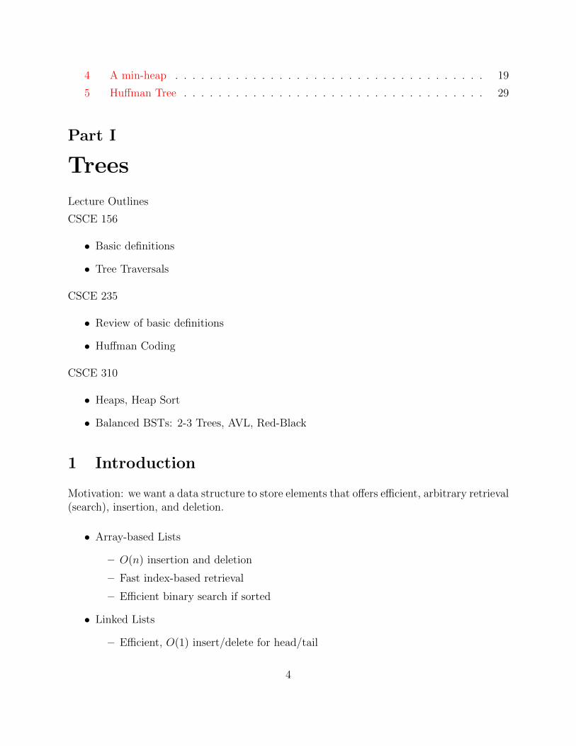
• A tree such that all nodes have at most two children is called a binary tree
• A binary tree is also oriented horizontally: each node may have a left and/or a rightchild
• Example: see Figure 1
• A path in a tree is a sequence nodes connected by edges
• The length of a path in a tree is the number of edges in the path (which equals thenumber of nodes in the path minus one)
• A path is simple if it does not traverse nodes more than once (this is the default typeof path)
• The depth of a node u is the length of the (unique) path from the root to u
• The depth of the root is 0
• The depth of a tree is the maximal depth of any node in the tree (sometimes the termheight is used)
5
• All nodes of the same depth are considered to be at the same level
• A binary tree is complete (also called full or perfect) if all nodes are present at all levels0 up to its depth d
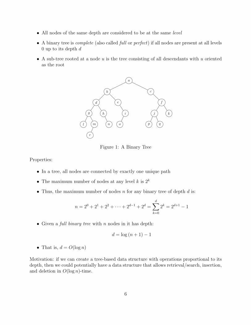
• A sub-tree rooted at a node u is the tree consisting of all descendants with u orientedas the root
a
b
d
g
l m
r
h
n
e
i
o
c
f
j
p q
k
Figure 1: A Binary Tree
Properties:
• In a tree, all nodes are connected by exactly one unique path
• The maximum number of nodes at any level k is 2k
• Thus, the maximum number of nodes n for any binary tree of depth d is:
n = 20 + 21 + 22 + · · ·+ 2d−1 + 2d =d∑
k=0
2k = 2d+1 − 1
• Given a full binary tree with n nodes in it has depth:
d = log (n+ 1)− 1
• That is, d = O(log n)
Motivation: if we can create a tree-based data structure with operations proportional to itsdepth, then we could potentially have a data structure that allows retrieval/search, insertion,and deletion in O(log n)-time.
6
3 Tree Traversal
• Given a tree, we need a way to enumerate elements in a tree
• Many algorithms exist to iterate over the elements in a tree
• We’ll look at several variations on a depth-first-search
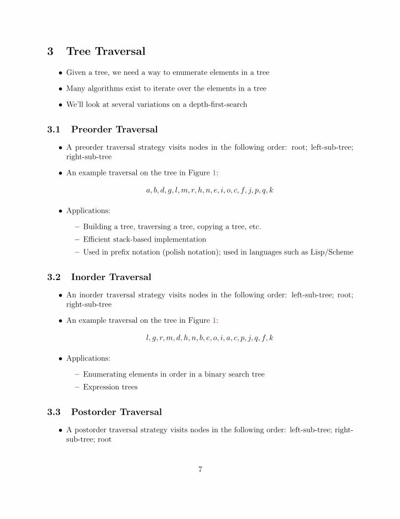
3.1 Preorder Traversal
• A preorder traversal strategy visits nodes in the following order: root; left-sub-tree;right-sub-tree
• An example traversal on the tree in Figure 1:
a, b, d, g, l,m, r, h, n, e, i, o, c, f, j, p, q, k
• Applications:
– Building a tree, traversing a tree, copying a tree, etc.
– Efficient stack-based implementation
– Used in prefix notation (polish notation); used in languages such as Lisp/Scheme
3.2 Inorder Traversal
• An inorder traversal strategy visits nodes in the following order: left-sub-tree; root;right-sub-tree
• An example traversal on the tree in Figure 1:
l, g, r,m, d, h, n, b, e, o, i, a, c, p, j, q, f, k
• Applications:
– Enumerating elements in order in a binary search tree
– Expression trees
3.3 Postorder Traversal
• A postorder traversal strategy visits nodes in the following order: left-sub-tree; right-sub-tree; root
7
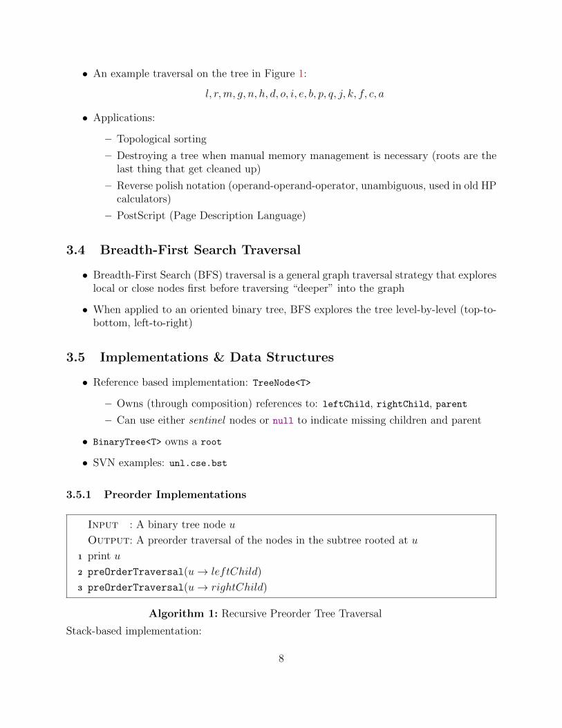
• An example traversal on the tree in Figure 1:
l, r,m, g, n, h, d, o, i, e, b, p, q, j, k, f, c, a
• Applications:
– Topological sorting
– Destroying a tree when manual memory management is necessary (roots are thelast thing that get cleaned up)
– Reverse polish notation (operand-operand-operator, unambiguous, used in old HPcalculators)
– PostScript (Page Description Language)
3.4 Breadth-First Search Traversal
• Breadth-First Search (BFS) traversal is a general graph traversal strategy that exploreslocal or close nodes first before traversing “deeper” into the graph
• When applied to an oriented binary tree, BFS explores the tree level-by-level (top-to-bottom, left-to-right)
3.5 Implementations & Data Structures
• Reference based implementation: TreeNode<T>
– Owns (through composition) references to: leftChild, rightChild, parent
– Can use either sentinel nodes or null to indicate missing children and parent
• BinaryTree<T> owns a root
• SVN examples: unl.cse.bst
3.5.1 Preorder Implementations
Input : A binary tree node u
Output: A preorder traversal of the nodes in the subtree rooted at u
1 print u
2 preOrderTraversal(u→ leftChild)
3 preOrderTraversal(u→ rightChild)
Algorithm 1: Recursive Preorder Tree Traversal
Stack-based implementation:
8
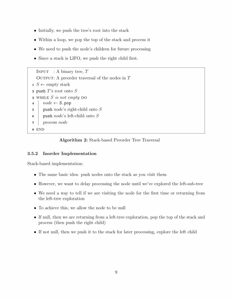
• Initially, we push the tree’s root into the stack
• Within a loop, we pop the top of the stack and process it
• We need to push the node’s children for future processing
• Since a stack is LIFO, we push the right child first.
Input : A binary tree, T
Output: A preorder traversal of the nodes in T
1 S ← empty stack
2 push T ’s root onto S
3 while S is not empty do4 node← S.pop
5 push node’s right-child onto S
6 push node’s left-child onto S
7 process node
8 end
Algorithm 2: Stack-based Preorder Tree Traversal
3.5.2 Inorder Implementation
Stack-based implementation:
• The same basic idea: push nodes onto the stack as you visit them
• However, we want to delay processing the node until we’ve explored the left-sub-tree
• We need a way to tell if we are visiting the node for the first time or returning fromthe left-tree exploration
• To achieve this, we allow the node to be null
• If null, then we are returning from a left-tree exploration, pop the top of the stack andprocess (then push the right child)
• If not null, then we push it to the stack for later processing, explore the left child
9
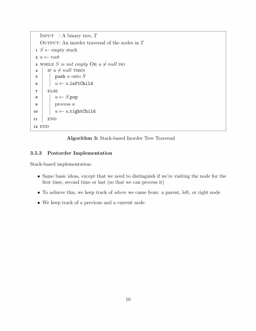
Input : A binary tree, T
Output: An inorder traversal of the nodes in T
1 S ← empty stack
2 u← root
3 while S is not empty Or u 6= null do4 if u 6= null then5 push u onto S
6 u← u.leftChild
7 else8 u← S.pop
9 process u
10 u← u.rightChild
11 end
12 end
Algorithm 3: Stack-based Inorder Tree Traversal
3.5.3 Postorder Implementation
Stack-based implementation:
• Same basic ideas, except that we need to distinguish if we’re visiting the node for thefirst time, second time or last (so that we can process it)
• To achieve this, we keep track of where we came from: a parent, left, or right node
• We keep track of a previous and a current node
10
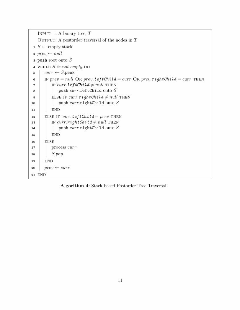
Input : A binary tree, T
Output: A postorder traversal of the nodes in T
1 S ← empty stack
2 prev ← null
3 push root onto S
4 while S is not empty do5 curr ← S.peek
6 if prev = null Or prev.leftChild = curr Or prev.rightChild = curr then7 if curr.leftChild 6= null then8 push curr.leftChild onto S
9 else if curr.rightChild 6= null then10 push curr.rightChild onto S
11 end
12 else if curr.leftChild = prev then13 if curr.rightChild 6= null then14 push curr.rightChild onto S
15 end
16 else17 process curr
18 S.pop
19 end
20 prev ← curr
21 end
Algorithm 4: Stack-based Postorder Tree Traversal
11
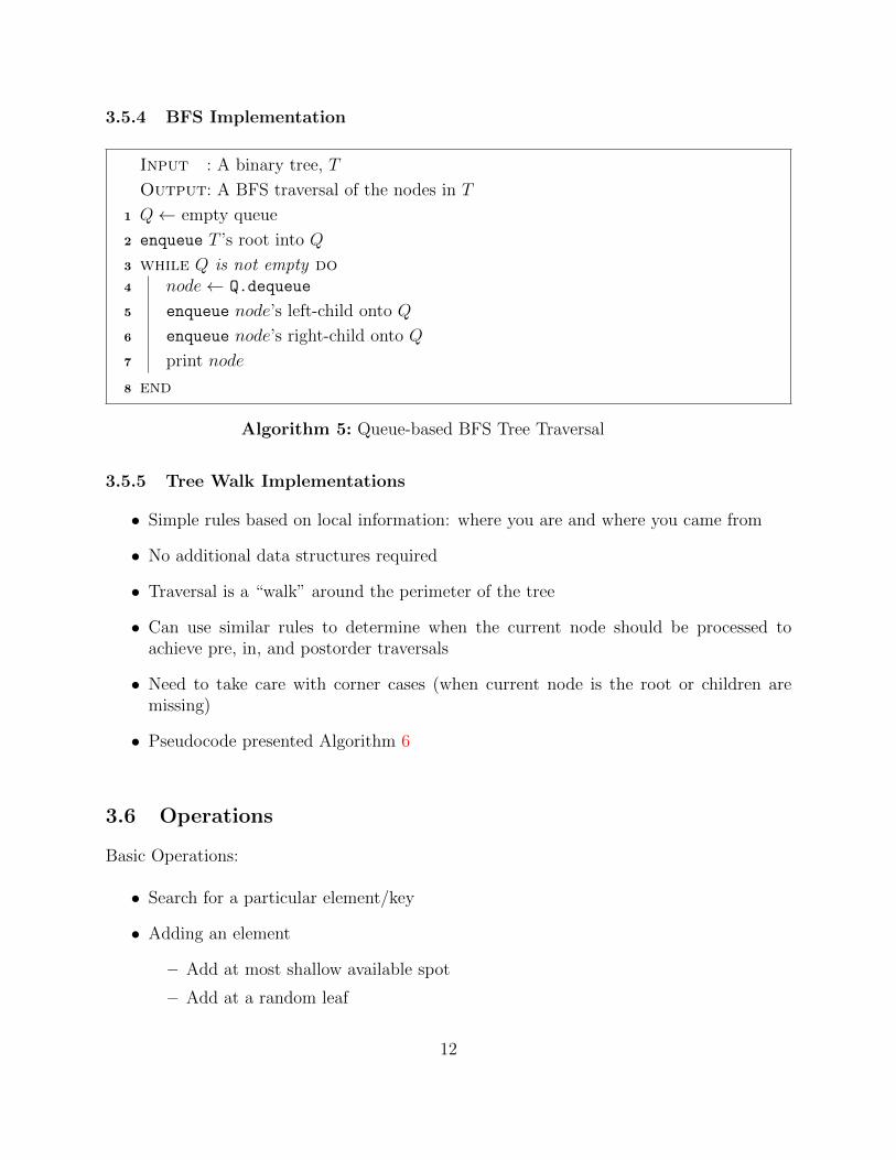
3.5.4 BFS Implementation
Input : A binary tree, T
Output: A BFS traversal of the nodes in T
1 Q← empty queue
2 enqueue T ’s root into Q
3 while Q is not empty do4 node← Q.dequeue
5 enqueue node’s left-child onto Q
6 enqueue node’s right-child onto Q
7 print node
8 end
Algorithm 5: Queue-based BFS Tree Traversal
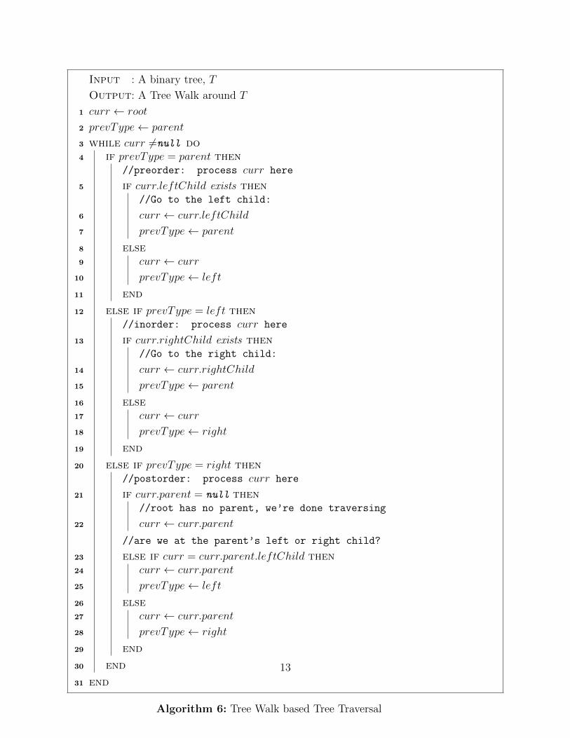
3.5.5 Tree Walk Implementations
• Simple rules based on local information: where you are and where you came from
• No additional data structures required
• Traversal is a “walk” around the perimeter of the tree
• Can use similar rules to determine when the current node should be processed toachieve pre, in, and postorder traversals
• Need to take care with corner cases (when current node is the root or children aremissing)
• Pseudocode presented Algorithm 6
3.6 Operations
Basic Operations:
• Search for a particular element/key
• Adding an element
– Add at most shallow available spot
– Add at a random leaf
12
Input : A binary tree, T
Output: A Tree Walk around T
1 curr ← root
2 prevType← parent
3 while curr 6=null do4 if prevType = parent then
//preorder: process curr here
5 if curr.leftChild exists then//Go to the left child:
6 curr ← curr.leftChild
7 prevType← parent
8 else9 curr ← curr
10 prevType← left
11 end
12 else if prevType = left then//inorder: process curr here
13 if curr.rightChild exists then//Go to the right child:
14 curr ← curr.rightChild
15 prevType← parent
16 else17 curr ← curr
18 prevType← right
19 end
20 else if prevType = right then//postorder: process curr here
21 if curr.parent = null then//root has no parent, we’re done traversing
22 curr ← curr.parent
//are we at the parent’s left or right child?
23 else if curr = curr.parent.leftChild then24 curr ← curr.parent
25 prevType← left
26 else27 curr ← curr.parent
28 prevType← right
29 end
30 end
31 end
Algorithm 6: Tree Walk based Tree Traversal
13
– Add internally, shift nodes down by some criteria
• Removing elements
– Removing leaves
– Removing elements with one child
– Removing elements with two children
Other Operations:
• Compute the total number of nodes in a tree
• Compute the total number of leaves in a tree
• Given an item or node, compute its depth
• Compute the depth of a tree
4 Binary Search Trees
Regular binary search trees have little structure to their elements; search, insert, deleteoperations are still linear with respect to the number of tree nodes, O(n). We want a datastructure with operations proportional to its depth, O(d). To this end, we add structure andorder to tree nodes.
• Each node has an associated key
• Binary Search Tree Property: For every node u with key uk in T
1. Every node in the left-sub-tree of u has keys less than uk
2. Every node in the right-sub-tree of u has keys greater than uk
• Duplicate keys can be handled, but you must be consistent and not guaranteed to becontiguous
• Alternatively: do not allow duplicate keys or define a key scheme that ensures a totalorder
• Inductive property: all sub-trees are also binary search trees
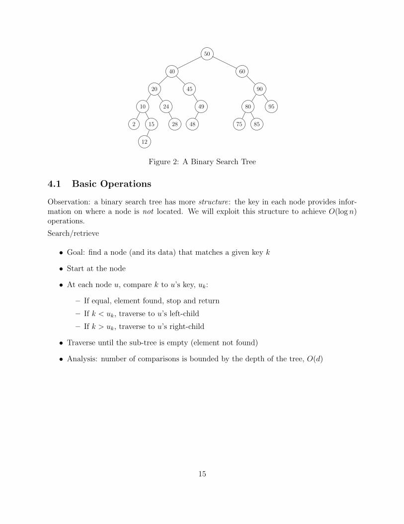
• A full example can be found in Figure 2
14
50
40
20
10
2 15
12
24
28
45
49
48
60
90
80
75 85
95
Figure 2: A Binary Search Tree
4.1 Basic Operations
Observation: a binary search tree has more structure: the key in each node provides infor-mation on where a node is not located. We will exploit this structure to achieve O(log n)operations.
Search/retrieve
• Goal: find a node (and its data) that matches a given key k
• Start at the node
• At each node u, compare k to u’s key, uk:
– If equal, element found, stop and return
– If k < uk, traverse to u’s left-child
– If k > uk, traverse to u’s right-child
• Traverse until the sub-tree is empty (element not found)
• Analysis: number of comparisons is bounded by the depth of the tree, O(d)
15
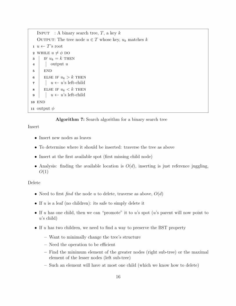
Input : A binary search tree, T , a key k
Output: The tree node u ∈ T whose key, uk matches k
1 u← T ’s root
2 while u 6= φ do3 if uk = k then4 output u
5 end
6 else if uk > k then7 u← u’s left-child
8 else if uk < k then9 u← u’s left-child
10 end
11 output φ
Algorithm 7: Search algorithm for a binary search tree
Insert
• Insert new nodes as leaves
• To determine where it should be inserted: traverse the tree as above
• Insert at the first available spot (first missing child node)
• Analysis: finding the available location is O(d), inserting is just reference juggling,O(1)
Delete
• Need to first find the node u to delete, traverse as above, O(d)
• If u is a leaf (no children): its safe to simply delete it
• If u has one child, then we can “promote” it to u’s spot (u’s parent will now point tou’s child)
• If u has two children, we need to find a way to preserve the BST property
– Want to minimally change the tree’s structure
– Need the operation to be efficient
– Find the minimum element of the greater nodes (right sub-tree) or the maximalelement of the lesser nodes (left sub-tree)
– Such an element will have at most one child (which we know how to delete)
16
– Delete it and store off the key/data
– Replace us key/data with the contents of the minimum/maximum element
• Analysis:
– Search/Find: O(d)
– Finding the min/max: O(d)
– Swapping: O(1)
– In total: O(d)
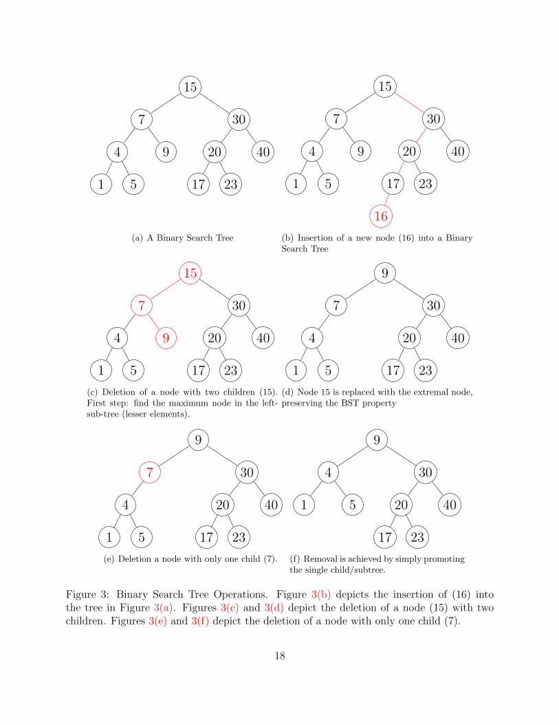
• Examples illustrated in Figure 3
5 Balanced Binary Search Trees
Motivation:
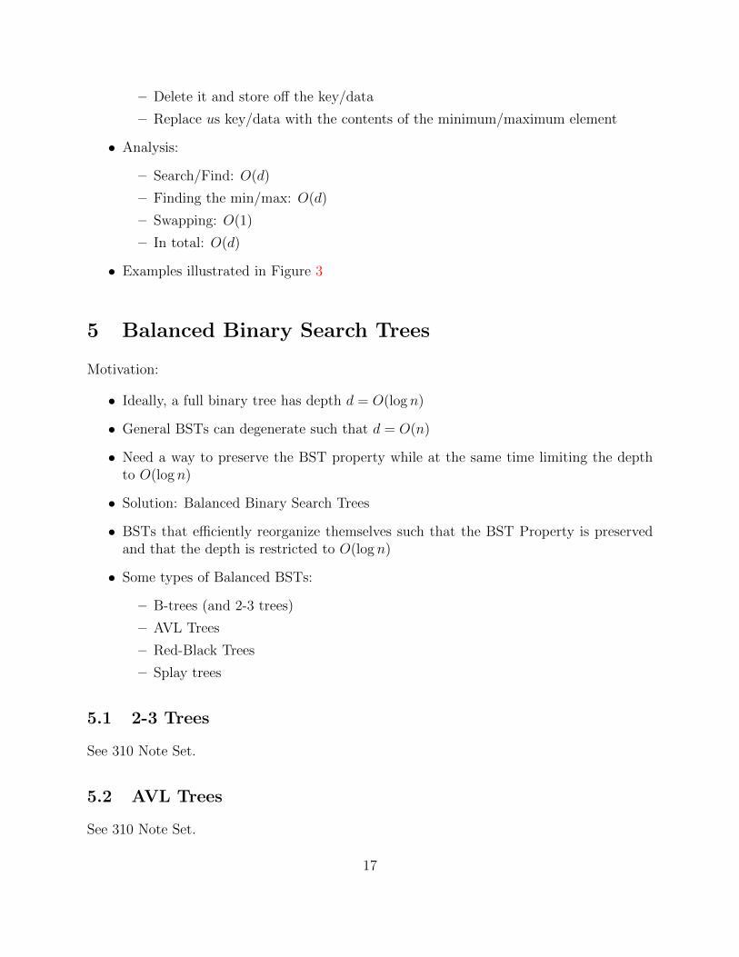
• Ideally, a full binary tree has depth d = O(log n)
• General BSTs can degenerate such that d = O(n)
• Need a way to preserve the BST property while at the same time limiting the depthto O(log n)
• Solution: Balanced Binary Search Trees
• BSTs that efficiently reorganize themselves such that the BST Property is preservedand that the depth is restricted to O(log n)
• Some types of Balanced BSTs:
– B-trees (and 2-3 trees)
– AVL Trees
– Red-Black Trees
– Splay trees
5.1 2-3 Trees
See 310 Note Set.
5.2 AVL Trees
See 310 Note Set.
17
15
7
4
1 5
9
30
20
17 23
40
(a) A Binary Search Tree
15
7
4
1 5
9
30
20
17
16
23
40
(b) Insertion of a new node (16) into a BinarySearch Tree
15
7
4
1 5
9
30
20
17 23
40
(c) Deletion of a node with two children (15).First step: find the maximum node in the left-sub-tree (lesser elements).
9
7
4
1 5
30
20
17 23
40
(d) Node 15 is replaced with the extremal node,preserving the BST property
9
7
4
1 5
30
20
17 23
40
(e) Deletion a node with only one child (7).
9
4
1 5
30
20
17 23
40
(f) Removal is achieved by simply promotingthe single child/subtree.
Figure 3: Binary Search Tree Operations. Figure 3(b) depicts the insertion of (16) intothe tree in Figure 3(a). Figures 3(c) and 3(d) depict the deletion of a node (15) with twochildren. Figures 3(e) and 3(f) depict the deletion of a node with only one child (7).
18
5.3 Red-Black Trees
See 310 Note Set.
6 Optimal Binary Search Trees
See 310 Note Set.
7 Heaps
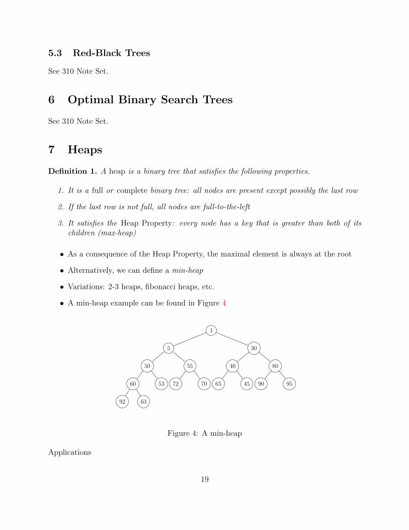
Definition 1. A heap is a binary tree that satisfies the following properties.
1. It is a full or complete binary tree: all nodes are present except possibly the last row
2. If the last row is not full, all nodes are full-to-the-left
3. It satisfies the Heap Property: every node has a key that is greater than both of itschildren (max-heap)
• As a consequence of the Heap Property, the maximal element is always at the root
• Alternatively, we can define a min-heap
• Variations: 2-3 heaps, fibonacci heaps, etc.
• A min-heap example can be found in Figure 4
1
5
50
60
92 63
53
55
72 70
30
40
65 45
80
90 95
Figure 4: A min-heap
Applications
19
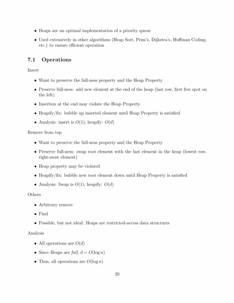
• Heaps are an optimal implementation of a priority queue
• Used extensively in other algorithms (Heap Sort, Prim’s, Dijkstra’s, Huffman Coding,etc.) to ensure efficient operation
7.1 Operations
Insert
• Want to preserve the full-ness property and the Heap Property
• Preserve full-ness: add new element at the end of the heap (last row, first free spot onthe left)
• Insertion at the end may violate the Heap Property
• Heapify/fix: bubble up inserted element until Heap Property is satisfied
• Analysis: insert is O(1); heapify: O(d)
Remove from top
• Want to preserve the full-ness property and the Heap Property
• Preserve full-ness: swap root element with the last element in the heap (lowest row,right-most element)
• Heap property may be violated
• Heapify/fix: bubble new root element down until Heap Property is satisfied
• Analysis: Swap is O(1); heapify: O(d)
Others
• Arbitrary remove
• Find
• Possible, but not ideal: Heaps are restricted-access data structures
Analysis
• All operations are O(d)
• Since Heaps are full, d = O(log n)
• Thus, all operations are O(log n)
20
7.2 Implementations
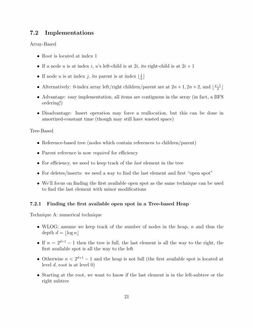
Array-Based
• Root is located at index 1
• If a node u is at index i, u’s left-child is at 2i, its right-child is at 2i+ 1
• If node u is at index j, its parent is at index b j2c
• Alternatively: 0-index array left/right children/parent are at 2n+ 1, 2n+ 2, and b j−12c
• Advantage: easy implementation, all items are contiguous in the array (in fact, a BFSordering!)
• Disadvantage: Insert operation may force a reallocation, but this can be done inamortized-constant time (though may still have wasted space)
Tree-Based
• Reference-based tree (nodes which contain references to children/parent)
• Parent reference is now required for efficiency
• For efficiency, we need to keep track of the last element in the tree
• For deletes/inserts: we need a way to find the last element and first “open spot”
• We’ll focus on finding the first available open spot as the same technique can be usedto find the last element with minor modifications
7.2.1 Finding the first available open spot in a Tree-based Heap
Technique A: numerical technique
• WLOG: assume we keep track of the number of nodes in the heap, n and thus thedepth d = blog nc
• If n = 2d+1 − 1 then the tree is full, the last element is all the way to the right, thefirst available spot is all the way to the left
• Otherwise n < 2d+1 − 1 and the heap is not full (the first available spot is located atlevel d, root is at level 0)
• Starting at the root, we want to know if the last element is in the left-subtree or theright subtree
21
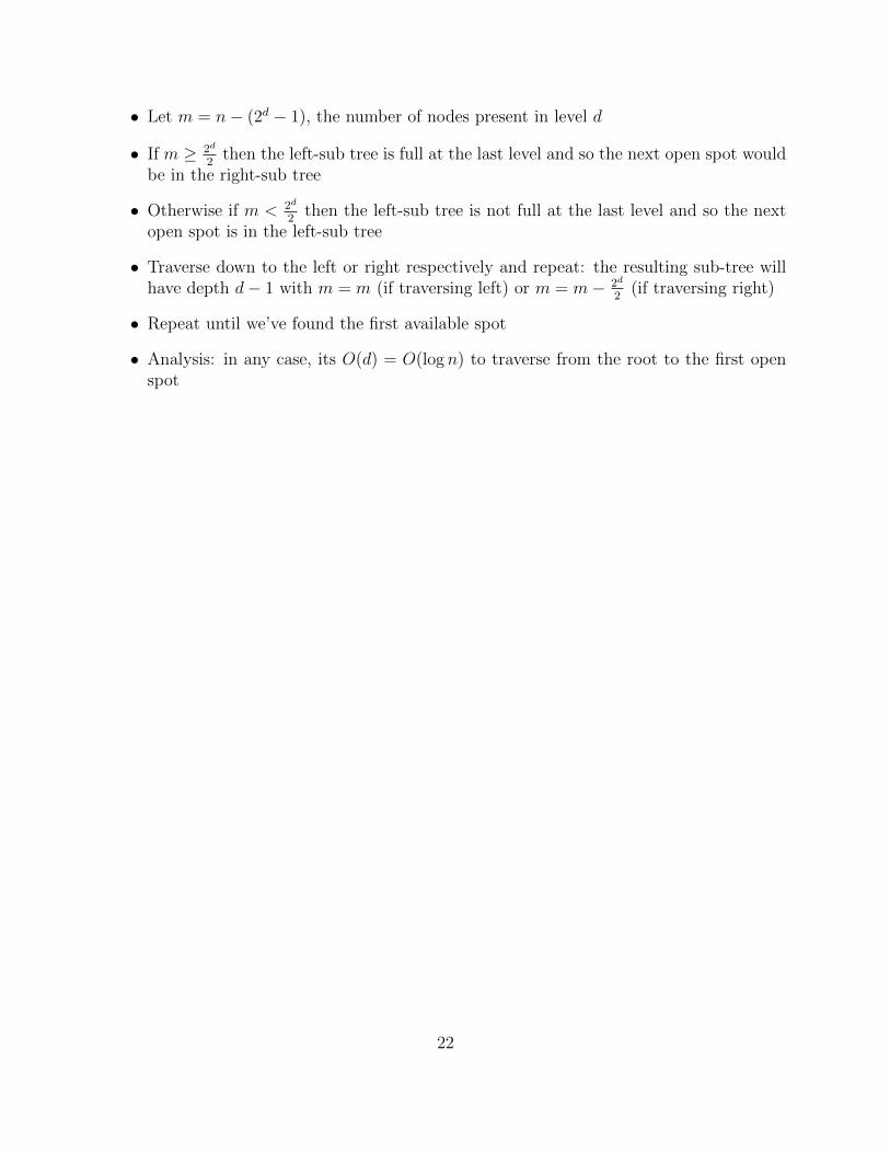
• Let m = n− (2d − 1), the number of nodes present in level d
• If m ≥ 2d
2then the left-sub tree is full at the last level and so the next open spot would
be in the right-sub tree
• Otherwise if m < 2d
2then the left-sub tree is not full at the last level and so the next
open spot is in the left-sub tree
• Traverse down to the left or right respectively and repeat: the resulting sub-tree willhave depth d− 1 with m = m (if traversing left) or m = m− 2d
2(if traversing right)
• Repeat until we’ve found the first available spot
• Analysis: in any case, its O(d) = O(log n) to traverse from the root to the first openspot
22
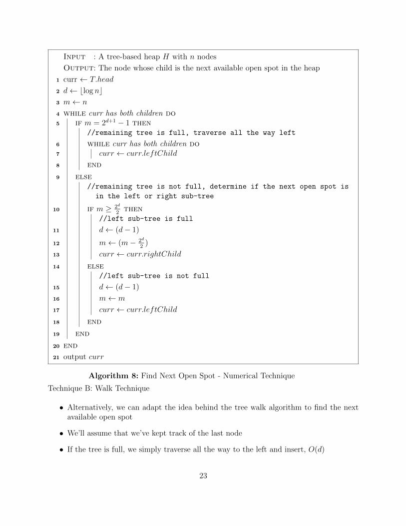
Input : A tree-based heap H with n nodes
Output: The node whose child is the next available open spot in the heap
1 curr ← T.head
2 d← blog nc3 m← n
4 while curr has both children do5 if m = 2d+1 − 1 then
//remaining tree is full, traverse all the way left
6 while curr has both children do7 curr ← curr.leftChild
8 end
9 else//remaining tree is not full, determine if the next open spot is
in the left or right sub-tree
10 if m ≥ 2d
2then
//left sub-tree is full
11 d← (d− 1)
12 m← (m− 2d
2)
13 curr ← curr.rightChild
14 else//left sub-tree is not full
15 d← (d− 1)
16 m← m
17 curr ← curr.leftChild
18 end
19 end
20 end
21 output curr
Algorithm 8: Find Next Open Spot - Numerical Technique
Technique B: Walk Technique
• Alternatively, we can adapt the idea behind the tree walk algorithm to find the nextavailable open spot
• We’ll assume that we’ve kept track of the last node
• If the tree is full, we simply traverse all the way to the left and insert, O(d)
23
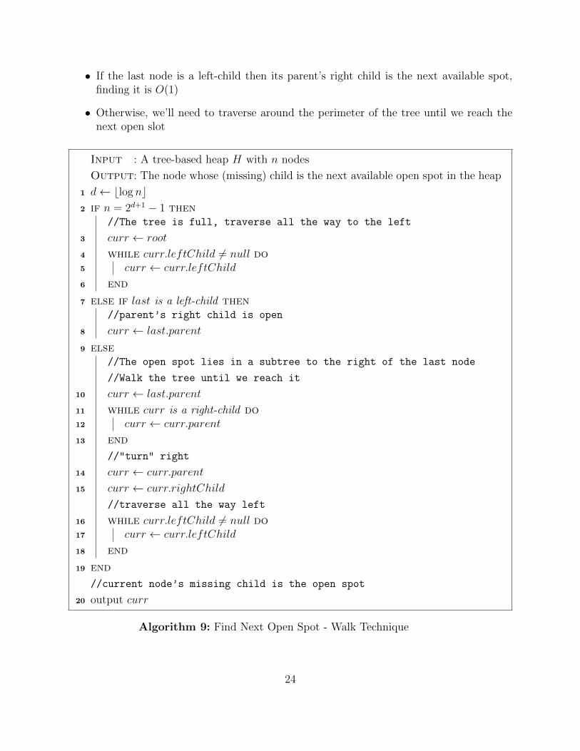
• If the last node is a left-child then its parent’s right child is the next available spot,finding it is O(1)
• Otherwise, we’ll need to traverse around the perimeter of the tree until we reach thenext open slot
Input : A tree-based heap H with n nodes
Output: The node whose (missing) child is the next available open spot in the heap
1 d← blog nc2 if n = 2d+1 − 1 then
//The tree is full, traverse all the way to the left
3 curr ← root
4 while curr.leftChild 6= null do5 curr ← curr.leftChild
6 end
7 else if last is a left-child then//parent’s right child is open
8 curr ← last.parent
9 else//The open spot lies in a subtree to the right of the last node
//Walk the tree until we reach it
10 curr ← last.parent
11 while curr is a right-child do12 curr ← curr.parent
13 end
//"turn" right
14 curr ← curr.parent
15 curr ← curr.rightChild
//traverse all the way left
16 while curr.leftChild 6= null do17 curr ← curr.leftChild
18 end
19 end
//current node’s missing child is the open spot
20 output curr
Algorithm 9: Find Next Open Spot - Walk Technique
24
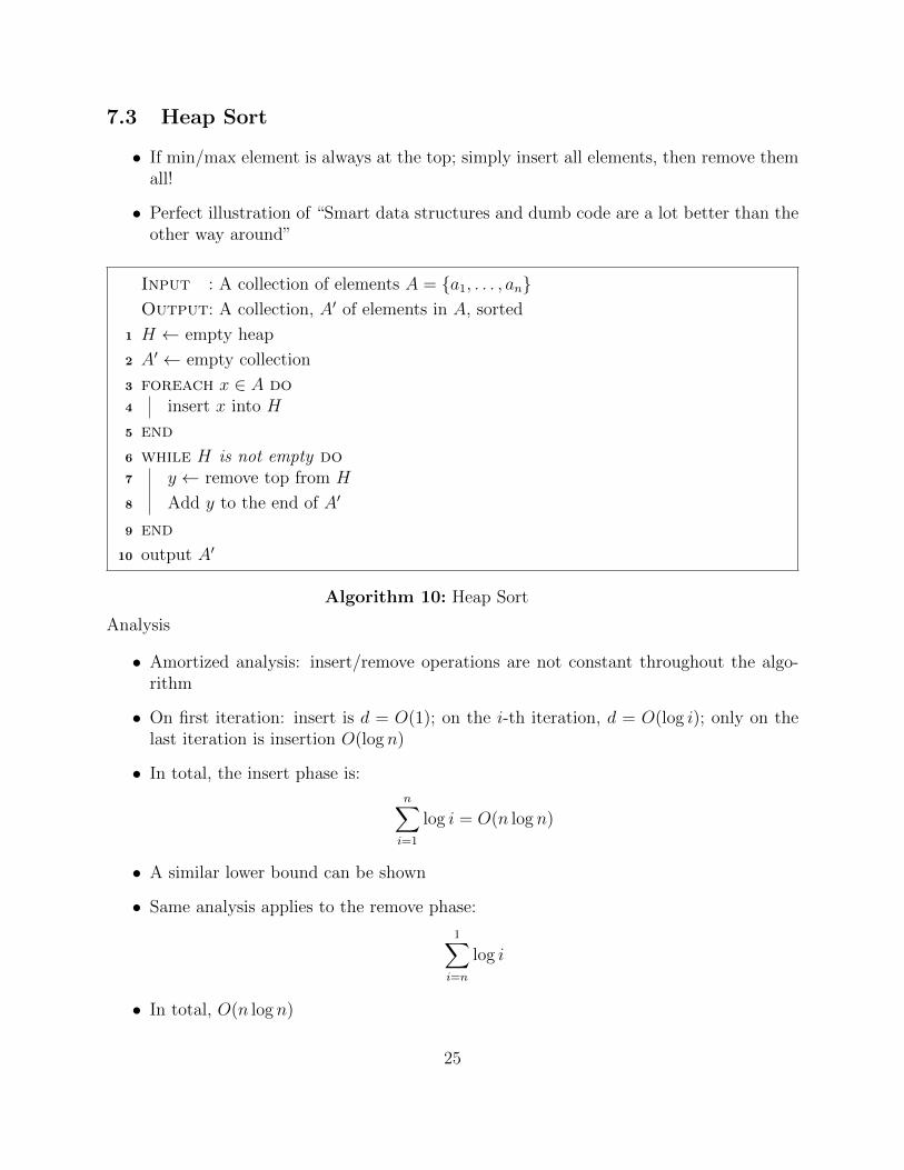
7.3 Heap Sort
• If min/max element is always at the top; simply insert all elements, then remove themall!
• Perfect illustration of “Smart data structures and dumb code are a lot better than theother way around”
Input : A collection of elements A = {a1, . . . , an}Output: A collection, A′ of elements in A, sorted
1 H ← empty heap
2 A′ ← empty collection
3 foreach x ∈ A do4 insert x into H
5 end
6 while H is not empty do7 y ← remove top from H
8 Add y to the end of A′
9 end
10 output A′
Algorithm 10: Heap Sort
Analysis
• Amortized analysis: insert/remove operations are not constant throughout the algo-rithm
• On first iteration: insert is d = O(1); on the i-th iteration, d = O(log i); only on thelast iteration is insertion O(log n)
• In total, the insert phase is:
n∑i=1
log i = O(n log n)
• A similar lower bound can be shown
• Same analysis applies to the remove phase:
1∑i=n
log i
• In total, O(n log n)
25
8 Java Collections Framework
Java has support for several data structures supported by underlying tree structures.
• java.util.PriorityQueue<E> is a binary-heap based priority queue
– Priority (keys) based on either natural ordering or a provided Comparator
– Guaranteed O(log n) time for insert (offer) and get top (poll)
– Supports O(n) arbitrary remove(Object) and search (contains) methods
• java.util.TreeSet<E>
– Implements the SortedSet interface; makes use of a Comparator
– Backed by TreeMap, a red-black tree balanced binary tree implementation
– Guaranteed O(log n) time for add, remove, contains operations
– Default iterator is an in-order traversal
9 Applications
9.1 Huffman Coding
Overview
• Coding Theory is the study and theory of codes—schemes for transmitting data
• Coding theory involves efficiently padding out data with redundant information toincrease reliability (detect or even correct errors) over a noisy channel
• Coding theory also involves compressing data to save space
– MP3s (uses a form of Huffman coding, but is information lossy)
– jpegs, mpegs, even DVDs
– pack (straight Huffman coding)
– zip, gzip (uses a Ziv-Lempel and Huffman compression algorithm)
Basics
• Let Σ be a fixed alphabet of size n
• A coding is a mapping of this alphabet to a collection of binary codewords,
Σ→ {0, 1}∗
26
• A block encoding is a fixed length encoding scheme where all codewords have the samelength (example: ASCII); requires dlog2 ne length codes
• Not all symbols have the same frequency, alternative: variable length encoding
• Intuitively: assign shorter codewords to more frequent symbols, longer to less frequentsymbols
• Reduction in the overall average codeword length
• Variable length encodings must be unambiguous
• Solution: prefix free codes : a code in which no whole codeword is the prefix of another(other than itself of course).
• Examples:
– {0, 01, 101, 010} is not a prefix free code.
– {10, 010, 110, 0110} is a prefix free code.
• A simple way of building a prefix free code is to associate codewords with the leavesof a binary tree (not necessarily full).
• Each edge corresponds to a bit, 0 if it is to the left sub-child and 1 to the right sub-child.
• Since no simple path from the root to any leaf can continue to another leaf, then weare guaranteed a prefix free coding.
• Using this idea along with a greedy encoding forms the basis of Huffman Coding
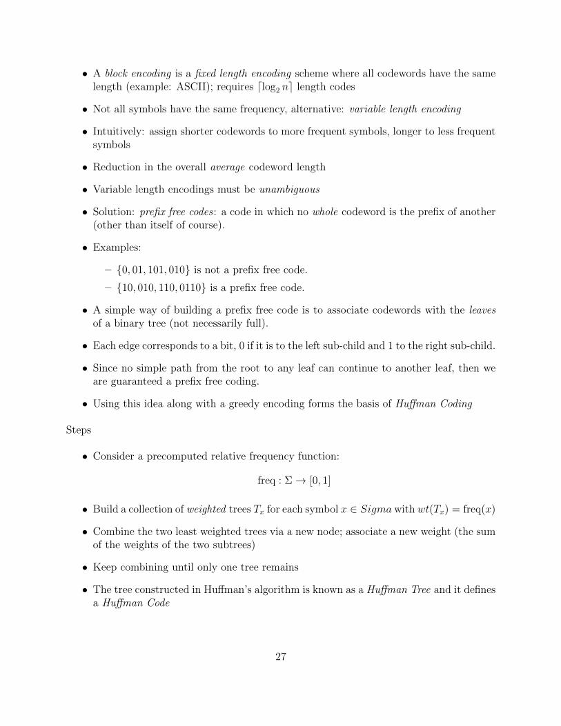
Steps
• Consider a precomputed relative frequency function:
freq : Σ→ [0, 1]
• Build a collection of weighted trees Tx for each symbol x ∈ Sigma with wt(Tx) = freq(x)
• Combine the two least weighted trees via a new node; associate a new weight (the sumof the weights of the two subtrees)
• Keep combining until only one tree remains
• The tree constructed in Huffman’s algorithm is known as a Huffman Tree and it definesa Huffman Code
27
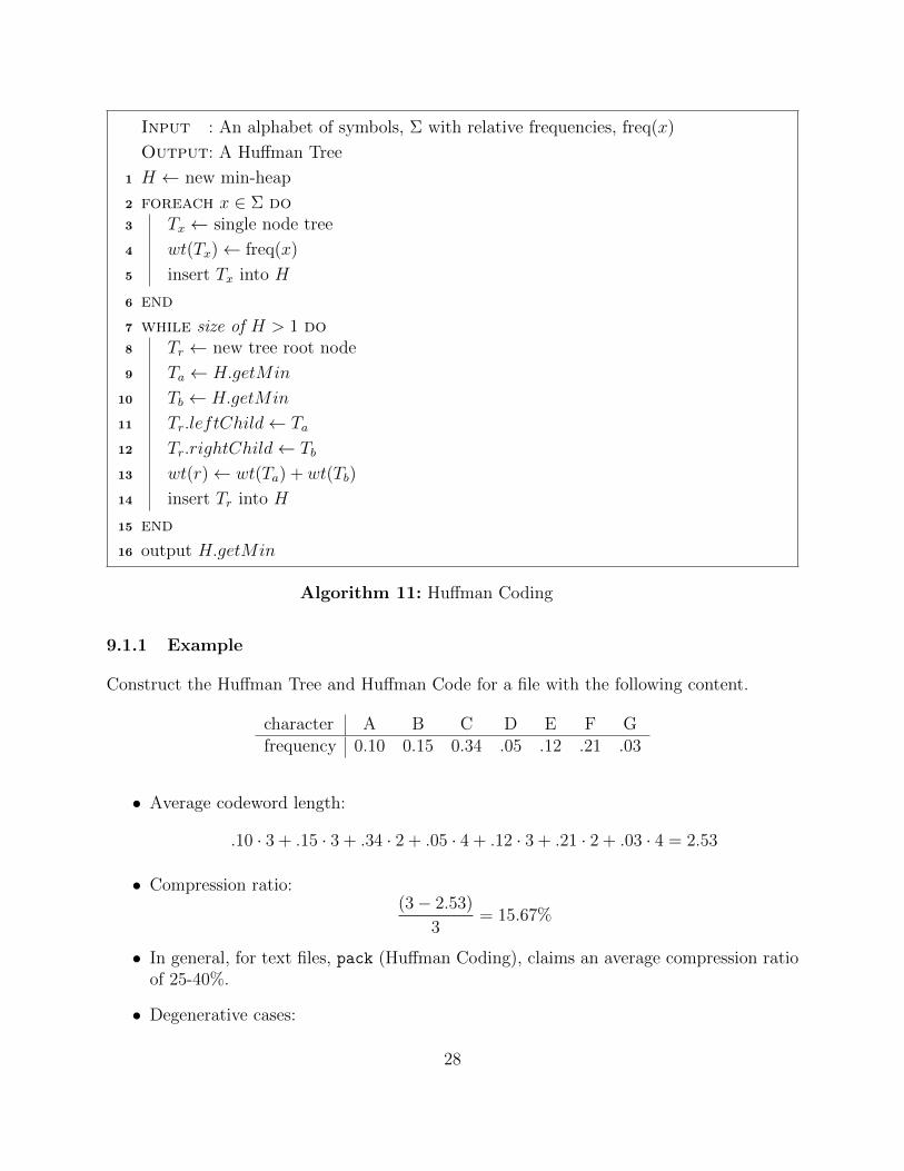
Input : An alphabet of symbols, Σ with relative frequencies, freq(x)
Output: A Huffman Tree
1 H ← new min-heap
2 foreach x ∈ Σ do3 Tx ← single node tree
4 wt(Tx)← freq(x)
5 insert Tx into H
6 end
7 while size of H > 1 do8 Tr ← new tree root node
9 Ta ← H.getMin
10 Tb ← H.getMin
11 Tr.leftChild← Ta
12 Tr.rightChild← Tb
13 wt(r)← wt(Ta) + wt(Tb)
14 insert Tr into H
15 end
16 output H.getMin
Algorithm 11: Huffman Coding
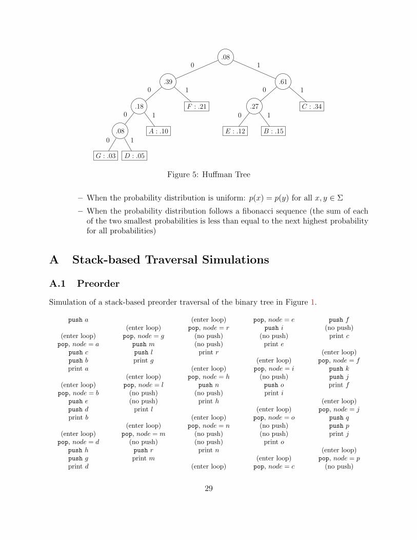
9.1.1 Example
Construct the Huffman Tree and Huffman Code for a file with the following content.
character A B C D E F Gfrequency 0.10 0.15 0.34 .05 .12 .21 .03
• Average codeword length:
.10 · 3 + .15 · 3 + .34 · 2 + .05 · 4 + .12 · 3 + .21 · 2 + .03 · 4 = 2.53
• Compression ratio:(3− 2.53)
3= 15.67%
• In general, for text files, pack (Huffman Coding), claims an average compression ratioof 25-40%.
• Degenerative cases:
28
.08
.39
.18
.08
G : .03
0
D : .05
1
0
A : .10
1
0
F : .21
1
0
.61
.27
E : .12
0
B : .15
1
0
C : .34
1
1
Figure 5: Huffman Tree
– When the probability distribution is uniform: p(x) = p(y) for all x, y ∈ Σ
– When the probability distribution follows a fibonacci sequence (the sum of eachof the two smallest probabilities is less than equal to the next highest probabilityfor all probabilities)
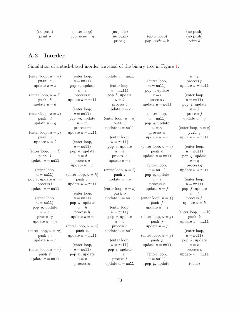
A Stack-based Traversal Simulations
A.1 Preorder
Simulation of a stack-based preorder traversal of the binary tree in Figure 1.
push a
(enter loop)pop, node = a
push cpush bprint a
(enter loop)pop, node = b
push epush dprint b
(enter loop)pop, node = d
push hpush gprint d
(enter loop)pop, node = g
push mpush lprint g
(enter loop)pop, node = l
(no push)(no push)
print l
(enter loop)pop, node = m
(no push)push rprint m
(enter loop)pop, node = r
(no push)(no push)
print r
(enter loop)pop, node = h
push n(no push)
print h
(enter loop)pop, node = n
(no push)(no push)
print n
(enter loop)
pop, node = epush i
(no push)print e
(enter loop)pop, node = i
(no push)push oprint i
(enter loop)pop, node = o
(no push)(no push)
print o
(enter loop)pop, node = c
push f(no push)
print c
(enter loop)pop, node = f
push kpush jprint f
(enter loop)pop, node = j
push qpush pprint j
(enter loop)pop, node = p
(no push)
29
(no push)print p
(enter loop)pop, node = q
(no push)(no push)
print q(enter loop)pop, node = k
(no push)(no push)
print k
A.2 Inorder
Simulation of a stack-based inorder traversal of the binary tree in Figure 1.
(enter loop, u = a)push a
update u = b
(enter loop, u = b)push b
update u = d
(enter loop, u = d)push d
update u = g
(enter loop, u = g)push g
update u = l
(enter loop, u = l)push l
update u = null
(enter loop,u = null)
pop l, update u = lprocess l
update u = null
(enter loop,u = null)
pop g, updateu = g
process gupdate u = m
(enter loop, u = m)push m
update u = r
(enter loop, u = r)push r
update u = null
(enter loop,u = null)
pop r, updateu = r
process rupdate u = null
(enter loop,u = null)
pop m, updateu = m
process mupdate u = null
(enter loop,u = null)
pop d, updateu = d
process dupdate u = h
(enter loop, u = h)push h
update u = null
(enter loop,u = null)
pop h, updateu = h
process hupdate u = n
(enter loop, u = n)push n
update u = null
(enter loop,u = null)
pop n, updateu = n
process n
update u = null
(enter loop,u = null)
pop b, updateu = b
process bupdate u = e
(enter loop, u = e)push e
update u = null
(enter loop,u = null)
pop e, updateu = e
process eupdate u = i
(enter loop, u = i)push i
update u = o
(enter loop, u = o)push o
update u = null
(enter loop,u = null)
pop o, updateu = o
process oupdate u = null
(enter loop,u = null)
pop i, updateu = i
process iupdate u = null
(enter loop,u = null)
pop i, updateu = i
process iupdate u = null
(enter loop,u = null)
pop a, updateu = a
process aupdate u = c
(enter loop, u = c)push c
update u = null
(enter loop,u = null)
pop c, updateu = c
process cupdate u = f
(enter loop, u = f)push f
update u = j
(enter loop, u = j)push j
update u = p
(enter loop, u = p)push p
update u = null
(enter loop,u = null)
pop p, update
u = pprocess p
update u = null
(enter loop,u = null)
pop j, updateu = j
process jupdate u = q
(enter loop, u = q)push q
update u = null
(enter loop,u = null)
pop q, updateu = q
process qupdate u = null
(enter loop,u = null)
pop f , updateu = f
process fupdate u = k
(enter loop, u = k)push k
update u = null
(enter loop,u = null)
pop k, updateu = k
process kupdate u = null
(done)
30
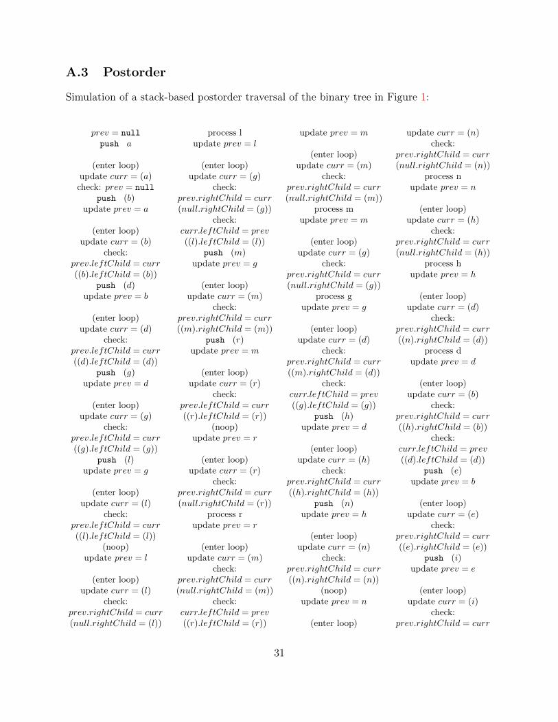
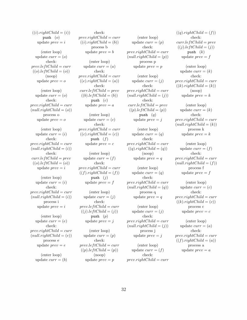
A.3 Postorder
Simulation of a stack-based postorder traversal of the binary tree in Figure 1:
prev = null
push a
(enter loop)update curr = (a)check: prev = null
push (b)update prev = a
(enter loop)update curr = (b)
check:prev.leftChild = curr((b).leftChild = (b))
push (d)update prev = b
(enter loop)update curr = (d)
check:prev.leftChild = curr((d).leftChild = (d))
push (g)update prev = d
(enter loop)update curr = (g)
check:prev.leftChild = curr((g).leftChild = (g))
push (l)update prev = g
(enter loop)update curr = (l)
check:prev.leftChild = curr((l).leftChild = (l))
(noop)update prev = l
(enter loop)update curr = (l)
check:prev.rightChild = curr(null.rightChild = (l))
process lupdate prev = l
(enter loop)update curr = (g)
check:prev.rightChild = curr(null.rightChild = (g))
check:curr.leftChild = prev((l).leftChild = (l))
push (m)update prev = g
(enter loop)update curr = (m)
check:prev.rightChild = curr((m).rightChild = (m))
push (r)update prev = m
(enter loop)update curr = (r)
check:prev.leftChild = curr((r).leftChild = (r))
(noop)update prev = r
(enter loop)update curr = (r)
check:prev.rightChild = curr(null.rightChild = (r))
process rupdate prev = r
(enter loop)update curr = (m)
check:prev.rightChild = curr(null.rightChild = (m))
check:curr.leftChild = prev((r).leftChild = (r))
update prev = m
(enter loop)update curr = (m)
check:prev.rightChild = curr(null.rightChild = (m))
process mupdate prev = m
(enter loop)update curr = (g)
check:prev.rightChild = curr(null.rightChild = (g))
process gupdate prev = g
(enter loop)update curr = (d)
check:prev.rightChild = curr((m).rightChild = (d))
check:curr.leftChild = prev((g).leftChild = (g))
push (h)update prev = d
(enter loop)update curr = (h)
check:prev.rightChild = curr((h).rightChild = (h))
push (n)update prev = h
(enter loop)update curr = (n)
check:prev.rightChild = curr((n).rightChild = (n))
(noop)update prev = n
(enter loop)
update curr = (n)check:
prev.rightChild = curr(null.rightChild = (n))
process nupdate prev = n
(enter loop)update curr = (h)
check:prev.rightChild = curr(null.rightChild = (h))
process hupdate prev = h
(enter loop)update curr = (d)
check:prev.rightChild = curr((n).rightChild = (d))
process dupdate prev = d
(enter loop)update curr = (b)
check:prev.rightChild = curr((h).rightChild = (b))
check:curr.leftChild = prev((d).leftChild = (d))
push (e)update prev = b
(enter loop)update curr = (e)
check:prev.rightChild = curr((e).rightChild = (e))
push (i)update prev = e
(enter loop)update curr = (i)
check:prev.rightChild = curr
31
((i).rightChild = (i))push (o)
update prev = i
(enter loop)update curr = (o)
check:prev.leftChild = curr((o).leftChild = (o))
(noop)update prev = o
(enter loop)update curr = (o)
check:prev.rightChild = curr(null.rightChild = (o))
process oupdate prev = o
(enter loop)update curr = (i)
check:prev.rightChild = curr(null.rightChild = (i))
check:curr.leftChild = prev((o).leftChild = (o))
update prev = i
(enter loop)update curr = (i)
check:prev.rightChild = curr(null.rightChild = (i))
process iupdate prev = i
(enter loop)update curr = (e)
check:prev.rightChild = curr(null.rightChild = (e))
process eupdate prev = e
(enter loop)update curr = (b)
check:prev.rightChild = curr((i).rightChild = (b))
process bupdate prev = b
(enter loop)update curr = (a)
check:prev.rightChild = curr((e).rightChild = (a))
check:curr.leftChild = prev((b).leftChild = (b))
push (c)update prev = a
(enter loop)update curr = (c)
check:prev.rightChild = curr((c).rightChild = (c))
push (f)update prev = c
(enter loop)update curr = (f)
check:prev.rightChild = curr((f).rightChild = (f))
push (j)update prev = f
(enter loop)update curr = (j)
check:prev.leftChild = curr((j).leftChild = (j))
push (p)update prev = j
(enter loop)update curr = (p)
check:prev.leftChild = curr((p).leftChild = (p))
(noop)update prev = p
(enter loop)update curr = (p)
check:prev.rightChild = curr(null.rightChild = (p))
process pupdate prev = p
(enter loop)update curr = (j)
check:prev.rightChild = curr(null.rightChild = (j))
check:curr.leftChild = prev((p).leftChild = (p))
push (q)update prev = j
(enter loop)update curr = (q)
check:prev.rightChild = curr((q).rightChild = (q))
(noop)update prev = q
(enter loop)update curr = (q)
check:prev.rightChild = curr(null.rightChild = (q))
process qupdate prev = q
(enter loop)update curr = (j)
check:prev.rightChild = curr(null.rightChild = (j))
process jupdate prev = j
(enter loop)update curr = (f)
check:prev.rightChild = curr
((q).rightChild = (f))check:
curr.leftChild = prev((j).leftChild = (j))
push (k)update prev = f
(enter loop)update curr = (k)
check:prev.rightChild = curr((k).rightChild = (k))
(noop)update prev = k
(enter loop)update curr = (k)
check:prev.rightChild = curr(null.rightChild = (k))
process kupdate prev = k
(enter loop)update curr = (f)
check:prev.rightChild = curr(null.rightChild = (f))
process fupdate prev = f
(enter loop)update curr = (c)
check:prev.rightChild = curr((k).rightChild = (c))
process cupdate prev = c
(enter loop)update curr = (a)
check:prev.rightChild = curr((f).rightChild = (a))
process aupdate prev = a
32