1

Trends in Rainfall and Runoff in the Blue Nile Basin: 1964-2003

Zelalem K. Tesemma1, Yasir A. Mohamed

2, 3, Tammo S. Steenhuis

1,4

1 Integrated Watershed Management and Hydrology Master’s Program, Cornell University, Bahir Dar,

Ethiopia.

2 International Water Management Institute, IWMI-NBEA, PO Box 5689, Addis Ababa, Ethiopia.

3 UNESCO-IHE Institute for Water Education, P.O. Box 3015, 2601DA Delft, Netherlands.

4 Biological and Environmental Engineering, Cornell University, Ithaca, NY 14853, USA.

Abstract

Most Nile water originates in Ethiopia but there is no agreement on how land degradation or climate

change affects the future flow in downstream countries. The objective of this paper is to improve

understanding of future conditions by analyzing historical trends. During the period 1963 to 2003, average

monthly basin wide precipitation and monthly discharge data were collected and analyzed statistically for

two stations in the upper 30% of Blue Nile Basin and one station at the Sudan-Ethiopia border. A rainfall

runoff model examined the causes for observed trends. The results show that while there was no significant

trend in the seasonal and annual basin-wide average rainfall, significant increases in discharge during the

long rainy season (June to September) at all three stations were observed. In the upper Blue Nile the short

rainy season flow (March to May), increased while the dry season flow (October to February) stayed the

same. At the Sudan border the dry season flow decreased significantly with no change in the short rainy

season flow. The difference in response was likely due to weir construction in the nineties at the Lake

Tana outlet that affected significantly the upper Blue Nile discharge but only affected less than 10% of the

discharge at the Sudan border. The rainfall runoff model reproduced the observed trends, assuming that an

additional ten percent of the hillsides were eroded in the 40 year time span and generated overland flow

instead of interflow and base flow. Models concerning future trends in the Nile cannot assume that the

landscape runoff processes will remain static.

Key words: Climate change, Watershed hydrology, Model, Rainfall-Runoff models, Blue Nile.

2

Introduction

The Nile basin is one of the most water-limited

basins in the world. Without the Nile major

portions of Sudan and Egypt would run out of

water. There is a growing anxiety about climate-

induced changes of the river’s discharge,

especially because Ethiopia, which generates

85% of the annual Main Nile flow (Sutcliffe and

Parks, 1999), is actively planning major

hydropower and irrigation development. To

develop appropriate adaptation strategies to relay

these concerns, long-term trends in stream flow

should be investigated (Conway, 2000; Conway

and Hulme, 1993 1996; Yilma and Demarce,

1995; Kim et al., 2008), which requires a better

understanding of the basin’s hydrology and

embedded long-term variability

The literature shows an increasing number of

climate change studies in the Nile basin (e.g.,

Conway and Hulme 1993, 1993; Conway, 2000;

Elshamy et al., 2009; Strzepek et al., 1996; Kim

et al., 2008). Impact of climate change on Blue

Nile discharge was highly variable in these

studies. One of the reasons is that the Global

Circulation Models cannot even agree on the

sign(s) of change (Elshamy et al., 2009).

Therefore, predicting future scenarios by

studying past trends of rainfall and discharge can

be an effective method. (Yilma and Demarce,

1995;; Kim, 2008; Conway, 2000) especially if

these trends can be related to changes in land use

and rainfall.

Previous studies employed simple linear

regressions over time to detect trends in annual

runoff and rainfall series without removing the

seasonal effects or trying to predict seasonal

differences in discharge (Conway, 2000;

Sutcliffe and Parks, 1999). The objective of this

research is therefore to improve on these

predictions by using both the Mann-Kendall and

Sen’s T test to detect trends in both seasonal and

annual runoff and rainfall and then using a semi-

distributed rainfall runoff model to both confirm

that the rainfall runoff relationship is changing

over to forty year period and to find the

underlying physical conditions that explains the

observed runoff trends.

The Blue Nile Basin

The Upper Blue Nile River (named Abbay in

Ethiopia) starts at Lake Tana and ends at the

Ethiopia-Sudan border. The topography of the

Blue Nile is composed of highlands, hills,

valleys and occasional rock peaks. Most of the

streams feeding the Blue Nile are perennial. The

average annual rainfall varies between 1200 and

3

1800 mm/yr (Figure 1 a), ranging from an

average of about 1000 mm/year near the

Ethiopia/Sudan border,to1400 mm/yr in the

upper part of the basin, and in excess of 1800

mm/yr in the south within Dedessa subbasin

(Conway 2000; Sutcliffe and Parks, 1999).

Locally the climatic seasons are defined as: dry

season (Bega) from October to the end of

February; short rain period (Belg) from March to

May; and long rainy period (Kiremt) from June

to September, with the greatest rainfall occurring

in July and August. The year to year variation in

monthly rainfall is most pronounced in the dry

season, with the lowest annual variation

occurring in the rainy season. Interannual

variability of rainfall in the basin is 10% (Table

1).

Table 1: The seasonal Mann-Kendall and Sen’s T tests statistics for Upper Blue Nile basin hydroclimatology record from1963 to 2003.

UB Station Seasons Mean1 CV2 (%)

z Test3 T test4 Slope5 (106 m3 / yr)

Change6 (Billion m3)

Change7 (%)

Rainfall

( mm)

Areal rainfall Annual 1286 10 -0.5 -0.5 Dry 151 36 -0.6 -1.1

Short rainy 218 26 0.6 0.5 Long rainy 916 10 -0.2 -0.7

Runoff

( ( Billion m3)

Bahir Dar Annual 3.8 36 2.0 3.3 Dry 2.0 33 0.6 0.9 Short rainy 0.3 100 3.2 2.4 2.1 0.08 33 Long rainy 1.5 45 2.7 2.6 9.8 0.39 26 Kessie Annual 16.0 31 2.2 3.8 109.0 4.36 27 Dry 3.2 30 0.8 1.0 Short rainy 0.6 60 3.2 3.2 7.2 0.288 51 Long rainy 12.2 35 3.6 2.7 83.7 3.35 27 El Diem Annual 46.9 20 0.5 0.3 Dry 11.0 32 -2.5 -2.4 -28.3 -1.13 -10 Short rainy 1.3 34 0.8 0.7 Long rainy 34.6 19 3.0 2.0 87.7 3.52 10

Note: Bold figures are significant at 5% significance level. Dry season (Oct-Feb); Short rainy season (March-May); Long rainy season (June – September) 1= Mean of the seasonal total runoff/rainfall (1964-2003). 2= coefficient of variation (1964-2003). 3=the Mann-Kendall test statistics. 4=Sen’s T test statistics. 5=Sen’s slope estimator. 6=calculated as slope times years of record (40 years). 7=calculated as change over the respective mean seasonal runoff

4

The long-term (1912-2003) mean annual

discharge of Blue Nile entering Sudan and

measured at Roseires/El Diem is 48.9 *109 m3/yr

which is about 60% of the flow of Main Nile

(Sutcliffe and Parks, 1999), with flows of

3.9*109 m3/yr at Bahir Dar (1959-2003) and 16.3

*109 m3/yr at Kessie (1953-2003) respectively

(Figure 1b). The distribution of seasonal

discharge varies considerably (Figure 1c). The

average discharge at El Diem is smallest in April

and greatest in August, about 35 times the April

flow. The annual variability of stream flow

varies

by less than 20% (Conway and Hulme, 1993;

Conway, 2000; Yilma and Demarce, 1995).

Most of the soil types covering the Blue Nile

basin are volcanic vertisols or latosols (Conway,

1997). There is uncertainty about how forest

cover has changed over the last 50 years. Some

report a decrease (USBR, 1964; Mohammed,

2007) while Bewket (2002) showed that green

cover has increased since 1950 over the 364 km2

Chemoga watershed in the upper Blue Nile

basin.

Input for statistical analysis and rainfall

runoff modeling

Input Data

Monthly data were collected for statistical

analysis, and modeling required 10-day data.

Monthly rainfall data for statistical analysis were

downloaded from Global Historical Climatology

Network (NOAA, 2009) and the 10-day rainfall

data for the selected stations (shown in Figure 2)

were obtained from the National Meteorological

Services Agency of Ethiopia. Monthly stream

5

flow data were obtained from the Hydrology

Department of the Ministry of Water Resources

of Ethiopia, and Ministry of Irrigation and Water

Resources of Sudan and the Global Hydro

Climate Data Network operated by

UNESCO/IHP available at

http://dss.ucar.edu/datasets/ds553.2/data/. From

the data available, three stream flow gages

(Figure 2) were selected that had more than 25

years data, which is sufficiently long to yield

statistically valid trends (Burn and Elnur, 2002).

Of these, the gaging station at El Deim at the

Sudanese Ethiopian border had the longest and

most reliable record, extending from 1912 to

present (Conway, 2000; Sutcliffe and Parks,

1999). The Kessie hydrometric station is located

near the bridge where the main road to Addis

Ababa from Bahir Dar crosses the Abbay (Blue

Nile) river, with discharge data recorded since

1953. Except for the last few years during the

bridge construction, the data is fair to good

(Conway, 2000). The third station is downstream

of the outlet of Lake Tana in Bahir Dar. The

construction in 1996 of the Chara-Chara weir for

generating hydropower has affected the

discharge by storing water in Lake Tana during

the wet season and releasing it during dry season.

Data validation and completion

After the raw rainfall and discharge data were

collected, a thorough checking and validation

was performed. First the data were visually

screened, and mistyped numbers and misplaced

decimal digits were fixed. Outliers were

identified by comparison with upper and a lower

boundary limits. Values outside the limits were

further validated by comparing the data plots of

neighboring stations. The confirmed suspect

values were removed and replaced by values

derived by a relation curve with neighboring

station(s). Missing data of the rainfall were fitted

using best fit regression with neighboring

stations.

Methodology

Both statistical analysis and a semi-distributed

rainfall runoff model were used to assess trends

in the discharge in the Blue Nile basin. The

statistical analysis of trends in climate and

hydrologic variables uses the Mann-Kendall test

(Zhang et al, 2001; Huth and Pokorna, 2004;

Harry et al, 1999). To gain more confidence in

our results, a categorically different and less

common technique, Sen’s T test, was employed

as well (KarabÖrk, 2007). Both tests are non-

parametric approaches and do not require any

assumptions about the distribution of the

variables.

6

Mann-Kendall test

The Mann-Kendall (Mann, 1945; Kendall, 1975)

test is a rank-based method that has been applied

widely to identify trends in hydroclimatic

variables (see e.g., Kahya and Kalayci, 2004; Xu

et al., 2003; Partal and Kalya, 2006; Yue and

Hashimoto, 2003). Following Burn et al. (2004),

we have corrected the data for

serial correlation through a modified version of

the Trend Free Pre-Whitening (TFPW) approach

developed by Zhang et al. (2001) and Yue et al.

(2002). The TFPW approach attempts to separate

the serial correlation that arises from a linear

trend from the original time series. This involves

estimating a monotonic trend for the series,

removing this trend prior to Pre-Whitening the

series and finally adding the monotonic trend

back to the Pre-Whitened data series to remove

the serial correlation.

Sen’s T test

The test statistic “T” is computed under the null

hypothesis of no trend, the distribution of T tends

toward normality with mean Zero and unit

variance (Sen, 1968a, b). The detailed

computational procedure of the test statistic is

given in Van Belle and Hughes, (1984).

All the trend results in this paper have been

evaluated at the 5% level of significance to

ensure an effective exploration of the trend

characteristics within the study area. The 5-

percent level of significance indicates that a 5-

percent chance for error exists in concluding that

a trend is statistically significant when in fact no

trend exists.

Rainfall-Runoff modeling

Statistical tests examine rainfall and discharge

separately. Rainfall runoff models can establish,

if the relationship between rainfall and discharge

has changed over time and may indicate the

underlying physical mechanisms if a change has

occurred.

The runoff model used here is a semi distributed

rainfall-runoff model (validated by Steenhuis et

al., 2009 for the Blue Nile Basin) in which

various portions of the watershed become

hydrologically active after the dry season when a

threshold moisture content is exceeded. In the

model, the permeable hillslope contribute rapid

subsurface flow (called interflow) and base

flow.. For each of the three regions, a

Thornthwaite Mather-type water balance is

calculated. Surface runoff is generated when the

soil is saturated and assumed to be at outlet

7

within the time step. The percolation is

calculated as any rainfall when the hillside soil is

at field capacity. Zero and first order reservoirs

determine the amount of water reaching the

outlet. Equations are given in Steenhuis et al.

(2009) and reproduced in the auxiliary material

in Appendix A.

Two types of input data are needed: climate and

landscape. Climate input data consisted of 10-

day rainfall amounts that were obtained by

averaging the 10-daily rainfall of the selected 10

rainfall gauging stations using the Thiessien

polygon method (Kim et al., 2008). The potential

evaporation was set according to Steenhuis et al

(2009) at values of 3.5 mm/day for the long rainy

season (June to September) and 5 mm/day for

the dry season (October to May). These values

were selected based on the long-term average of

available potential evaporation data over the

basin. As landscape input parameters for the

model, the relative areas of the three regions are

needed as well as the amount of water (available

for evaporation) between wilting point and the

threshold moisture content. In addition, the

interflow and baseflow rate constants were part

of the input data set. The landscape parameter

values cannot be determined a priori and need to

be obtained by calibration.

Calibration was performed by manually

changing the parameter values in small steps

around the values found earlier by Steenhuis et al

(2009) for the Blue Nile basin. The model was

calibrated for two three-year periods 34 years

apart: 1964-1966 and 1998- 2000. Validation

was done in the subsequent three years for each

period: 1967-1969 and 2001-2003. To test if the

parameter values had changed over the 34 year

period, the calibrated parameters set for the early

period was compared with the observed flow for

the later period. Similarly the calibrated data for

the latter period was run for the early period.

Results and Discussion

Trend analysis results

The annual areal rainfall over the basin (CV =

10%) is less variable (column 4 in Table 1) than

the stream flow at all the stations. The opposite

is true for the dry (October to February) and

short rainy season (March to May) while the

long rainy season(June to September)

precipitation is less variable than the rainfall

Precipitation: Both the Mann-Kendall and Sen’s

T indicate that there was no significant trend

level in the basin wide annual, dry season, short

and long rainy season rainfall at 5% significant

level for the Blue Nile basin for the period from

8

1963-2004 (column 5 & 6 of Table 1) Our results

are in agreement with Conway (2000) who did

not find either a tendency towards wet or dry

condition.

Discharge: The trends in stream flow computed

by the Mann-Kendall test and Sen’s T test are

similar (Table 1). The agreement of the two

different tests shows that the results are robust

and both indicate that there was no significant

trend in the observed annual runoff at El Diem at

the Sudan border. This is consistent with the

observation at that point that the basin-wide

annual rainfall remained the same and potential

evaporation from year to year usually does not

vary. The annual discharge, therefore, which is

the difference between rainfall and evaporation -

a unique function of rainfall and potential

evaporation- should stay the same for a given

annual rainfall amount. Somewhat surprising is

the fact that the annual discharge at Kessie (with

1/3 the discharge at El Diem) and Bahir Dar

increased significantly by about 25 percent over

the 40 year period.

Despite the difference in annual trends, all three

stations show significant increasing discharges

over time during the long wet season. As a

percentage of the 40-year seasonal mean, these

increments were 26% at Bahir Dar, 27% at

Kessie and 10% at El Diem. Discharge during

the short rainy season stream increased

significantly at 33% at Bahir Dar and 51% at

Kessie, while the trend was not significant at El

Diem in the period from 1963 to 2003 (Table 1).

The possible reason for this phenomena could be

analysis of low values may retrieve drastic

results and effect of the Chara-Chara weir after

1996. Finally, the dry season stream flow

showed no significant trends at Bahir Dar and

Kessie but a significant decreasing trend at El

Diem by 10% (Table 1). Despite differences in

rainfall pattern, the analysis clearly shows

differences in runoff pattern over the 40 year

period. For the two upper Nile stations, Kessie

and Bahir Dar the increased annual discharge is a

consequence of the increased discharge during

the two rainy periods while the dry season flow

is not affected. For El Deim, where the annual

flow remained constant over the 40 years, the

increase in discharge during the wet season is

canceled by a decrease of flow during the dry

period. The results at Kessie and Bahir Dar

(especially during low flow conditions) are

affected by installation of the Chara Chara weir

at the outlet of Lake Tana during the last 7 years

of the record analyzed, which increased flow

during the dry season to provide water for the

hydropower plant at the Nile Falls. It also

decreased the flow during the rainy season but,

9

despite that, the discharge during the rainy

period still increased according to our analysis.

Our results for the Upper Blue Nile agree in part

with those of Bewket and Sterk (2005) in the

Chemoga watershed, which is not affected by

Chara-Chara weir where during the wet season

the discharge increased with time but decreased

during the dry season, giving creditability to the

assumed effect of the Chara Chara weir on

increasing the low flows.

Rainfall Runoff simulation

Rainfall-Runoff modeling can establish if the

relationship between rainfall and runoff are exist.

In addition, underlying hydrological mechanisms

for altered discharge can be identified (Mishra et

al., 2004). Since the flow at Bahir Dar and

Kessie is most affected by the Chara-Chara weir,

we used the gauge at El Diem to establish the

relationship. Calibration of the parameters was

based on the assumption the subsurface flow

parameters (interflow and baseflow) remain the

same over time, as does the storage of the

landscape components. Thus the only calibration

parameter to characterize the flow in the 1960’s

and at the end of the 1990’s is the amount of

degraded soils that produce surface runoff in the

1990’s and around 2000. The calibrated

parameter values are shown in Table 2. For the

1964-1969 the observed and predicted values

correspond most closely when the hillside

(recharging the interflow and groundwater) made

up 70% of the landscape and with a soil water

storage of 250 mm (between wilting point and

field capacity). Surface runoff was produced

from the exposed surface or bedrock making up

10% of the landscape and saturated areas

comprising 20% of the area (Table 2, Figure 3).

After the dry season, the exposed bedrock

needed to fill up a storage of 25 mm before it

became hydrologically active, whereas the

saturated areas required 200 mm. Parameter

calibration for the period from 1998 to 2000

showed that increasing exposed bedrock

coverage to 20% and decreasing the hillslopes by

10% to 60% gave the best fit while all other

parameters could be kept the same (Table 2,

Figure 3). The Nash-Sutcliffe model efficiencies

were remarkably high for such a simple model:

0.92 and 0.91 for the calibration periods and 0.87

and 0.86 for the validation periods, respectively

for the first and second time periods, (Table 3,

a). Similarly, good correlation coefficient r2, and

small Root Mean Square Errors were obtained

for selected set of calibration an validation

parameters (Table 3, a). The high runoff Nash-

Sutcliffe efficiencies are an indication that

although simple, the model effectively captured

the hydrological processes in which various

portions of the watershed become hydrologically

10

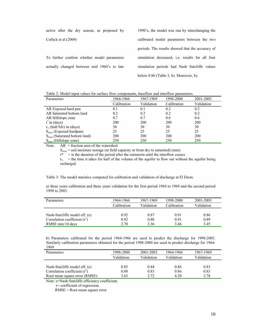
active after the dry season, as proposed by

Collick et al (2009)

To further confirm whether model parameters

actually changed between mid 1960’s to late

1990’s, the model was run by interchanging the

calibrated model parameters between the two

periods. The results showed that the accuracy of

simulation decreased, i.e. results for all four

simulation periods had Nash Sutcliffe values

below 0.86 (Table 3, b). Moreover, by

Table 2: Model input values for surface flow components, baseflow and interflow parameters.

Parameters 1964-1966 1967-1969 1998-2000 2001-2003 Calibration Validation Calibration Validation

AR Exposed hard pan 0.1 0.1 0.2 0.2 AR Saturated bottom land 0.2 0.2 0.2 0.2 AR Hillslope zone 0.7 0.7 0.6 0.6 t* in (days) 200 200 200 200 t½ (half life) in (days) 30 30 30 30 Smax (Exposed hardpan) 25 25 25 25 Smax (Saturated bottom land) 200 200 200 200 Smax (Hillslope zone) 250 250 250 250 Note: AR = fraction area of the watershed

Smax = soil moisture storage (at field capacity or from dry to saturated) (mm). t* = is the duration of the period after the rainstorm until the interflow ceases t½ = the time it takes for half of the volume of the aquifer to flow out without the aquifer being recharged.

Table 3: The model statistics computed for calibration and validation of discharge at El Diem. a) three years calibration and three years validation for the first period 1964 to 1969 and the second period 1998 to 2003. Parameters 1964-1966 1967-1969 1998-2000 2001-2003

Calibration Validation Calibration Validation Nash-Sutcliffe model eff. (e) 0.92 0.87 0.91 0.86 Correlation coefficient (r2) 0.92 0.88 0.91 0.89 RMSE mm/10 days 2.70 3.36 3.46 3.45

b) Parameters calibrated for the period 1964-1966 are used to predict the discharge for 1998-2003. Similarly calibration parameters obtained for the period 1998-2000 are used to predict discharge for 1964-1969 Parameters 1998-2000 2001-2003 1964-1966 1967-1969

Validation Validation Validation Validation Nash-Sutcliffe model eff. (e) 0.85 0.84 0.86 0.83 Correlation coefficient (r2) 0.88 0.83 0.86 0.83 Root mean square error (RMSE) 3.63 3.72 4.20 3.78 Note: e=Nash-Sutcliffe efficiency coefficient. r= coefficient of regression, RMSE = Root mean square error

11

comparing observed versus predicted discharge

in Figure 4 it becomes obvious that the calibrated

dataset of 1998-2000 period predicted earlier

runoff and greater peaks than observed for the

period of 1964-1969 (Figures 4a and 4b).

Similarly, the calibrated data set for the 1960’s

12

predicted later runoff and lower peaks than

observed around 2000 (Figures 4c and 4d). The

subsurface flow routines of the simple model are

not sufficiently sensitive to predict

the observed differences in base flow during the

dry season. Despite that this model is based on a

conceptual framework, it can be seen as

arithmetical relationship that relate the spatially

averaged ten-day rainfall to the ten-day

watershed discharge. This relationship between

rainfall and watershed discharge clearly changes

over the 40 year period (Figures 3 and 4)

13

indicating that the runoff mechanisms are

shifting due to landscape characteristics since the

precipitation did not vary. However but cannot

indicate what the reason is. The conceptual

framework is needed to find the underlying cause

for the observed shift in runoff pattern.

The conceptual framework leads to following

explanation for the alteration in the runoff

pattern: Soil erosion during the period from the

early 1960’s to 2000, although occurring over

the whole watershed, was more severe in certain

areas that caused the bedrock to be exposed. The

hillsides that were eroded in this period no

longer stored rainfall and released it later as

interflow as they had in the 1960’s but instead

produced surface runoff in 2000. This in turn

caused a greater portion of the watershed to

become hydrologically active at an earlier stage,

releasing more of the rainfall sooner resulting in

earlier flows and greater peak flow. These

simulation results are in line with the statistical

result at the El Diem site which shows increasing

trends of runoff during long or short rainy

seasons but decreasing dry season runoff, while

annual flow has no significant change (see Table

1).

Conclusions

Trends of precipitation and discharge over a 40

year period in Blue Nile basin have been

investigated. The results show the precipitation

did not change over the entire basin. Discharge

analysis for Bahir Dar and Kessie representing

the upper part of Blue Nile and El Diem at the

border between Sudan and Ethiopia shows that

annual discharge increased for the upper Blue

Nile only. Discharge during the long rainy

season increased at all three stations. Discharge

during the short rainy season increased due to the

influence of the Chara-Chara weir at the outlet of

Lake Tana.

A simple rainfall runoff model calibrated for the

beginning and end of the 40 year period showed

that the peak in the runoff occurred earlier at the

end of this period than the beginning. This could

be explained by erosion of hillside lands that

stored some of the water before it became eroded

and contributing areas of direct runoff. Further

research is needed if other factors than the

suggested changes could explain the statistical

and simulation results.

Acknowledgements

We extend sincere thanks to the Hydrology

Department of the Ministry of Water Resources

of Ethiopia and Sudan and the National

14

Meteorological Services Agency of Ethiopia for

kindly providing us with the stream flow and

rainfall data used for the study. We also would

like to thank Dr. Amy S. Collick for providing

materials and valuable comments. Financial

support was provided by IWMI project entitled:

‘Nile Basin Focal Project (NBFP).

References

Bewket, W. 2002. Land covers dynamics since the 1950s in Chemoga watershed, Blue Nile Basin, Ethiopia Mountain Research and Development 22(3): 263-269. Bewket, W. and Sterk, G. 2005. Dynamics in land covers and its effect on streamflow in the Chemoga watershed, Blue Nile basin, Ethiopia. Journal of Hydrol. Process. 19, 445-458.

Burn, D. H., Cunderlik, J. M. and Pietroniro, A. 2004. Hydrological trends and variability in the Liard River basin. Hydrological sciences Journal 49(1), 53-67.

Burn, D. H. and Elnur, M. A. 2002. Detection of hydrologic trend and variability. Journal of Hydrology 255, 107-122. Collick A. S., Easton Z. M., Asgaharie T., Biruk, B. Tilahun SAdgo E., Awulachew S. B. Zeleke G. and Steenhuis T. S. 2009. A simple semi-distributed water balance model FOr the Ethiopian Highlands. Hydrological processes. In press. Conway, D. and Hulme, M. 1993. Recent fluctuations in precipitation and runoff over the Nile sub-basins and their impact on main Nile discharge. Climatic Change 25, 127–151. Conway, D. and Hulme, M. 1996. The impacts of climate variability and future climate change in the Nile basin on water resources in Egypt. Water Resour. Dev. 12, 277–296. Conway, D. 1997. A water balance model of the Upper Blue Nile in Ethiopia. Hydrol. Sci. J. 42(2), 265–286. Conway, D. 2000. The climate and hydrology of the Upper Blue Nile River. The Geogr. J. 166, 49–62. Elshamy, M. E., Seierstad, I. A. and Sorteberg, A. 2009. Impacts of climate change on Blue Nile

flows using bias-corrected GCM scenarios. J. of Hydrol. Earth Syst. Sci., 13, 551–565. Harry, F., Lins and Slack, J. R. 1999. Streamflow trends in the United States. Geographical research letters vol. 26, No. 2, pages 227-230. Hirsch, R. M. and Slack, J. R. 1984. Non-parametric trend test for seasonal data with serial dependence. Water Resources Res. 20(6), 727-732. Hirsch, R. M., Slack, J. R. and Smith, R. A. 1982. Techniques of trend analysis for monthly water quality data, Water Resource Res.18 (1), 107-121. Huth, R. and Pokorna, L. 2004. Parametric versus non-parametric estimates of climatic trends. Theoretical and Applied Climatology 77, 107-112. Karabörk, M.C. 2007 Trends in drought patterns of Turkey. J. of Environmental Engineering and Science 6: 45-52. Kahya, E. and Kalayci, S. 2004. Trend analysis of streamflow in Turkey. J. of Hydrology 289: 128-144. Kendall, M. G. 1975. Rank correlation Methods, Charles Griffin, London. Kim, U., Kaluarachchi, J. J. and Smakhtin, V. U. 2008. Climate Change Impacts on Hydrology and Water Resources of the Upper Blue Nile River Basin, Ethiopia. Colombo, Sri Lanka: International Water Management Institute (IWMI) Research Report 126. 27 p. ISBN 978-92-9090-696-4. Mann, H.B., 1945. Nonparametric tests against trend, Econometrica, 13, 245-259. McHugh O.V. 2006. Integrated water resources assessment and management in a drought-prone watershed in the Ethiopian highlands. PhD dissertation, Department of Biological and

15

Environmental Engineering. Cornell University Ithaca NY. Mishra, A., Hata, T. and Abdelhadi, A. W. 2004. Models for Recession Flows in the Upper Blue Nile River. Hydrological Processes 18:2773-2786. Mohammed, A. 2007. Hydrological responses to land cover changes (Modelling Case study in Blue Nile basin, Ethiopia). M.Sc thesis, International Institute for Geo-information Science and Earth Observation. Enschede, the Netherlands. NOAA. 2009. Global Historical Climatology Network. ftp://ftp.ncdc.noaa.gov/pub/data/ghcn/v2/, last accessed September, 2009) Partal, T. and Kalya, E. 2006. Trend analysis in Turkish precipitation data. Hydrological Process 20, 2011-2026. Sen, P. K. 1968a. On a class of aligned rank order tests in two-way layouts. Annual Mathematics Statistic 39: 1115-1124. Sen, P. K. 1968b. Estimates of the regression coefficient based on Kendall’s tau. Journal of the American Statistical Association 39: 1379-1389. Steenhuis, T.S, A.S. Collick, Z. M. Easton, E. S. Leggesse, H. K. Bayabil, E. D. White, S.B. Awulachew, Enyew Adgo, A.A. Ahmed. 2009. Predicting discharge and sediment for the Abay (Blue Nile) with a simple model Hydroloical Processes 23: 3728-3737 Strzepek, K. M., Yates, D. N. and El Quosy D.E., 1996. Vulnerability assessment of water

resources in Egypt to climate change in the Nile Basin. Climate research 6, 89-95.3(2):98-108. Sutcliffe, J. V. and Parks, Y. P. 1999. The hydrology of the Nile, IAHS Special publication No.5 IAHS press, Institute of Hydrology, Wallingford, oxford shine. USBR (United State Bureau of Reclamation), 1964. Land and Water Resource of the Blue Nile Basin. Main report. United State Dept. Interior Bureau of Reclamation, Washington DC, USA. Van Belle, G., and Hughes, J. P., 1984. Nonparametric tests for trend in water quality. Water Resources Res. 20(1), 127-136. Yilma, S. and Demarce G. R. 1995. Rainfall variability in the Ethiopian and Eritrean highlands and its links with the southern oscillation index. Journal of Biogeography 22, 945-952. Yue, S. and Hashino, M. 2003. Long term trends of annual and monthly precipitation in Japan. Journal of the American Water Resources Association. 39, 587-596. Yue, S., Pilon, P., Phinney, B. and Cavadias, G. 2002. The influence of autocorrelation on the ability to detect trend in hydrological series. Hydrological Processes 16, 1807–1829. Xu, Z. X., Takeuchi, K. and Ishidaira, H. 2003. Monotonic trend and step changes in Japanese precipitation. Journal of Hydrology, 279, 144-150. Zhang, X., Harvey, K. D., Hogg, W. D. and Yuzyk, T.R. 2001. Trends in Canadian streamflow. Water Resources Res. 37(4), 987-998.

Auxiliary Material

APPENDIX A Rainfall runoff model

The landscape is divided into two parts, the well

drained hillslopes, and the relatively flatter areas

that become easily saturated during the rainfall

season. The hillslopes are further divided into

two parts that either are degraded or have highly

permeable soils above a restricted layer at some

depth. The degraded areas have the hardpan

exposed at the soil surface. In these areas that

have restricted infiltration, a small amount of

water can be stored before saturation excess

16

surface runoff occurs. On the highly permeable

portion of the hillslopes most of the water is

transported through subsurface as rapid

subsurface flow (e.g., interflow over a restrictive

layer) or base flow (percolated from the soil

profile to deeper soil and rock layers, McHugh,

2006). The flatter areas that drain the

surrounding hillslopes become runoff source

areas when saturated (Fig. A1 shows a schematic

representation of a simplified hillslope). Three

separate water balances are calculated. The water

balance for the each of the three areas can be

written as

[ ] tPREPttStS ercass ∆−−−+∆−= )()(

(A1)

Where P is rainfall (LT-1), Ea the actual

evapotranspiration (LT-1), Ss(t) is storage water

in the soil profile at time t (L) above the

restrictive layer, Ss(t-∆t) is previous time step

water storage (L), R is saturation excess runoff

(LT-1), Perc is percolation to the subsoil (LT-1)

and ∆t is the time step (10 days in our case).

Percolation occurs on the non degraded

hillslopes when the soil storage is more than

field capacity. Surface runoff on the saturated

bottom lands and degraded hill slopes occurs

when they are saturated is equal the amount

rainfall minus the water that is needed to fill up

the soil to saturation.

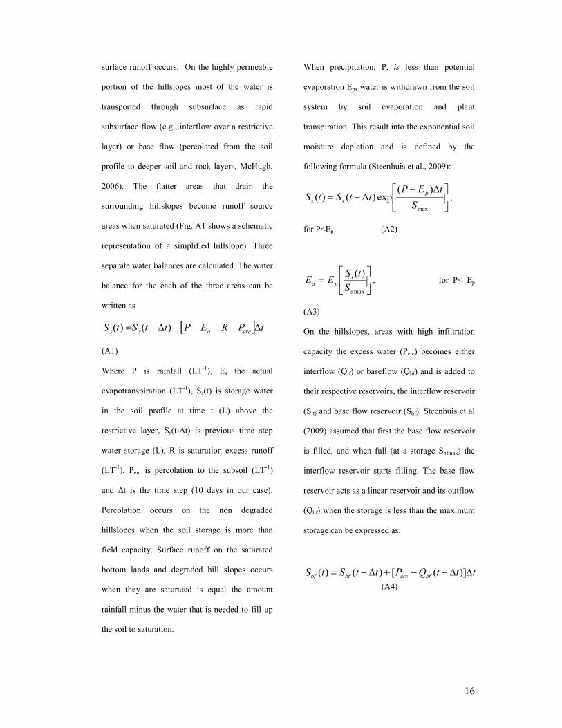
When precipitation, P, is less than potential

evaporation Ep, water is withdrawn from the soil

system by soil evaporation and plant

transpiration. This result into the exponential soil

moisture depletion and is defined by the

following formula (Steenhuis et al., 2009):

∆−∆−=

max

)(exp)()(

S

tEPttStS

p

ss ,

for P<Ep (A2)

=

max

)(

s

spaS

tSEE , for P< Ep

(A3)

On the hillslopes, areas with high infiltration

capacity the excess water (Perc) becomes either

interflow (Qif) or baseflow (Qbf) and is added to

their respective reservoirs, the interflow reservoir

(Sif) and base flow reservoir (Sbf). Steenhuis et al

(2009) assumed that first the base flow reservoir

is filled, and when full (at a storage Sbfmax) the

interflow reservoir starts filling. The base flow

reservoir acts as a linear reservoir and its outflow

(Qbf) when the storage is less than the maximum

storage can be expressed as:

tttQPttStS bfercbfbf ∆∆−−+∆−= )]([)()( (A4)

17

[ ]t

ttStQ

bf

bf ∆

∆−−=

]exp[1)()(

α

(A5)

Figure A1: Schematic for saturation excess overland flow, infiltration, interflow and baseflow for a characteristic hill slopes in the Blue Nile Basin (after Steenhuis et al., 2009)

where α is the reservoir coefficient (L-1) and is

equal to 0.69/t½. When baseflow storage (Sbf) is

full, the baseflow can be calculated by setting

Sbf(t)=Sbfmax in equation (A5). Equation (A4)

reduces so that the water entering the reservoir is

equal to what flows out calculated with equation

(A5). After the base flow reservoir filled, the

remaining percolation water fills up the interflow

flow reservoir started from the hillslopes by

gravity under these circumstances the flow

decreases linearly (i.e., a zero order reservoir)

after a recharge event. The total interflow at time

t can be obtained by superimposing the fluxes for

the individual events,

∑≤

=

−−=*

12

*

**

1)(2)(

ττ

τ ττ

ττtPtQ ercif , τ ≤ τ*

(A6)

where τ* is the duration of the period after the

rainstorm until the interflow ceases, Qif(t) is the

interflow at a time t, ����∗ �� � is the effective

percolation on day t-τ. The effective percolation

is defined as the total percolation minus the

amount needed for refilling the baseflow aquifer.

Refer to Steenhuis et al, (2009) for more details

on the model development. References are in the

main text