triangular spectral element simulation of two-dimensional ... · triangular spectral element...
TRANSCRIPT

Geophys. J. Int. (2006) 166, 679–698 doi: 10.1111/j.1365-246X.2006.03006.x
GJI
Sei
smol
ogy
Triangular Spectral Element simulation of two-dimensional elasticwave propagation using unstructured triangular grids
E. D. Mercerat,1,∗ J. P. Vilotte1 and F. J. Sanchez-Sesma2
1Laboratoire de Sismologie, Institut de Physique du Globe de Paris, France. E-mail: [email protected] de Ingenierıa, UNAM, Mexico
Accepted 2006 March 14. Received 2006 March 13; in original form 2005 July 11
S U M M A R YA Triangular Spectral Element Method (TSEM) is presented to simulate elastic wave prop-agation using an unstructured triangulation of the physical domain. TSEM makes use of avariational formulation of elastodynamics based on unstructured straight-sided triangles thatallow enhanced flexibility when dealing with complex geometries and velocity structures. Thedisplacement field is expanded into a high-order polynomial spectral approximation over eachtriangular subdomain. Continuity between the subdomains of the triangulation is enforced us-ing a multidimensional Lagrangian interpolation built on a set of Fekete points of the triangle.High-order accuracy is achieved by resorting to an analytical computation of the associatedinternal product and bilinear forms leading to a non-diagonal mass matrix formulation. There-fore, the time stepping involves the solution of a sparse linear algebraic system even in theexplicit case. In this paper the accuracy and the geometrical flexibility of the TSEM is explored.Comparison with classical spectral elements on quadrangular grids shows similar results interms of accuracy and stability even for long simulations. Surface and interface waves areshown to be accurately modelled even in the case of complex topography with the TSEM.Numerical results are presented for 2-D canonical examples as well as more specific problems,such as 2-D elastic wave scattering by a cylinder embedded in an homogeneous half-space.They all illustrate the enhanced geometrical flexibility of the TSEM. This clearly suggeststhe need of further investigations in computational seismology specifically targeted towardsefficient implementations of the TSEM both in the time and the frequency domain.
Key words: elastic waves, numerical simulation, spectral element method, triangular un-structured grids.
1 I N T RO D U C T I O N
Many problems in geophysics need to infer the physical and chem-
ical parameter distributions of the Earth’s interior from informa-
tion provided by seismic wave propagation through complex me-
dia. Moreover, numerical simulations of earthquake-induced wave
propagation within heterogeneous geological structures have im-
portant implications in terms of earthquake risk assessment and of
strong motion predictions. Continuous improvements during the last
decades, both in terms of acquisition techniques and seismic network
density, lead today the possibility of exploiting new information
provided by high-resolution multicomponent seismograms, over a
wide range of frequencies. The development of new seismic inter-
pretation methods, which take advantage of these high-resolution
∗Presently at: Laego-INERIS, Laboratoire Environnement Geomecanique
et Ouvrages, Ecole des Mines de Nancy, France.
observations, requires accurate numerical modelling tools for the
simulation of the complete waveform field in heterogeneous geo-
logical media with complex geometries.
Recent developments towards high-order numerical modelling of
seismic wave propagation (Seriani et al. 1992; Maggio et al. 1996;
Faccioli et al. 1997; Komatitsch & Vilotte 1998; Komatitsch et al.1999; Komatitsch & Tromp 1999; Komatitsch et al. 2000, 2001;
Chaljub et al. 2003; Capdeville et al. 2003; Komatitsch et al. 2004)
have been based on spectral element techniques (Patera 1984; Maday
& Patera 1989; Bernardi & Maday 1992). There are several reasons
for using spectral elements in computational seismology. First, by
means of piecewise continuous geometrical maps, spectral elements
have higher geometrical flexibility than spectral or pseudo-spectral
methods, which are mainly confined to smooth problems defined
on simple domains that can be mapped onto the nd-cube (where
nd is the space dimension), while retaining the spatial exponential
convergence for locally smooth solutions with quasi-optimal disper-
sion errors. Second, like low-order finite elements, spectral elements
are based on the weak form of elastodynamics that involve only
C© 2006 The Authors 679Journal compilation C© 2006 RAS
680 E. D. Mercerat, J. P. Vilotte and F. J. Sanchez-Sesma
first-order spatial derivatives. The weak formulation has the nice
property to handle naturally both interface continuity and free-
boundary conditions, allowing very accurate resolution of evanes-
cent interface and surface waves that are of major interest in seismol-
ogy. Finally, spectral elements are much easier to implement than
global spectral methods on today’s generation parallel computers,
which involve non-uniform distributed access to the memory.
Previous work with spectral element method (SEM) in computa-
tional seismology typically used explicit time stepping and quadri-
lateral elements, with a clever choice of the polynomial basis for the
function expansion based on the Legendre family of Jacobi polyno-
mials, and with a set of non-uniform collocation points defined as the
Gauss–Lobatto–Legendre (GLL) cardinal points with the associated
quadrature. Moreover, quadrangles allow the use of a tensor prod-
uct to construct the Lobatto–Legendre cardinal interpolation basis
(Bernardi & Maday 1992; Deville et al. 2002) in such a way that the
mass matrix remains diagonal with a time-step restriction scaling
as O(N−2), where N is the order of the polynomial basis, while the
derivatives can be calculated using an efficient sum-factorization
technique (Orszag 1980) at a cost of only O(E N α) with α = 3 and
α = 4 for 2-D and 3-D problems, respectively, and E the number
of elements. Apart from that, this method inherits the nice property
of the associated GLL quadrature allowing for the exact integra-
tion of polynomial functions of order 2N − 1, with only N + 1
points. Finally, straightforward C0 continuity of the kinematic field
can be insure while using conforming quadrangle meshes thanks
to the local conforming maps and the cardinal Lobatto–Legendre
interpolation basis.
The need for geometric flexibility is especially important in com-
putational seismology when dealing with complex wave phenom-
ena, such as the scattering by rough topographies of the Earth and
sea bottom surfaces, or the seismic response of sedimentary basins
with complex structures and fault geometries. Today, such flexibil-
ity is hardly achieved when using quadrangles for several reasons.
First, when using non-conforming grids, continuity between mis-
matched elements must be enforced in a variational sense by re-
sorting to the so-called mortar method (Bernardi et al. 1994; Ben
Belgacem 1999), which adds both programming complexity and
operation costs. Second, when resorting to unstructured meshes,
that is meshes referenced using only one index, very few robust
grid-generation software based on hexahedra are available today
and all of them have difficulties to handle rapid multiscale mesh
refinements and de-refinements. Third, the stability of explicit nu-
merical schemes can be strongly affected when using quadrangles
that are highly skewed, leading to non-uniform resolution and severe
time-step restrictions. Higher geometrical flexibility is, therefore, a
strong motivation for exploring the use of triangular elements and
unstructured meshes, an extension that has been investigated by
hp-finite element methods in these last decades using multivariate
Lagrangian interpolation (Chen & Babuska 1995).
Extension of SEMs to unstructured triangular meshes hinges upon
the application of more complex polynomial basis specifically tai-
lored to accurately approximate smooth functions defined on the
nd-simplex. Drawing on ideas from Orszag’s work on spherical har-
monics (Orszag 1974), and on orthogonal polynomial basis initially
derived by Proriol (1957) and Koorwinder (1975), Dubiner (1991)
first overcame these difficulties and obtained a tensor-product-like
spectral method for triangles based on Jacobi polynomials. In the
construction of such orthogonal polynomial basis, Dubiner makes
use of a non-rotational collapsed coordinate system, induced by the
mapping of each triangular region to a rectangle, and of the gen-
eralization of the direct tensor products by the so-called warped
tensor product. Dubiner’s basis has been extended to incompress-
ible Navier–Stokes equations in 3-D by Sherwin & Karniadakis
(1995a,b); Karniadakis & Sherwin (1999), and to geophysical fluid
dynamics problems by Wingate & Boyd (1996).
One possible approach relies on a modal hierarchical approx-
imation that has been extensively investigated by Sherwin &
Karniadakis (1995a,b, 1996); Karniadakis & Sherwin (1999). This
approach makes use of an almost orthogonal approximation basis,
based on the modification of the original Dubiner’s basis, which
separate interior and boundary contributions, in order to insure C0
continuity between the triangular subdomains. This so-called mod-
ified Dubiner’s basis (Dubiner 1991), and its interior-orthogonal
variant (Wingate & Boyd 1996), makes use of a triangular polyno-
mial truncation in modes {xnym, m + n ≤ N}, where N is the global
polynomial order of the expansion, together with an efficient warped
tensor product and a Gauss-type quadrature formula defined on a
squared-grid of points. This allows the backward transform to be
still computed in O(E N 4) in 3-D, and the forward transformation in
O(E Nq ), where Nq is the order of the quadrature. All the computa-
tions are done in the modal space. However in practice, as noted in
Hesthaven & Teng (2000), the quadrature formula is oversampled,
it uses more grid points than required by the order of the polyno-
mial basis. Even though the added complexity in the expression of
the modified basis allows for C0 continuity between the triangular
elements, such a construction still depends on the orientation of
the local coordinate system of the contributing elements. Moreover,
the partial orthogonality of the basis destroys much of the spar-
sity of the SEM matrices and leads to a non-diagonal mass matrix
(Warburton et al. 1999).
We investigate a second approach based on a nodal approxima-
tion (Taylor et al. 2000; Warburton et al. 2000; Hesthaven & Teng
2000; Bos et al. 2001). As in classical SEM, resorting to multivari-
ate Lagrange polynomial interpolation allows straightforward C0
continuity between triangular elements. It is worth noting here that
a modal expansion can always be represented as a Lagrange poly-
nomial expansion of equivalent order, defined on an appropriate set
of points, a fact efficiently used in classical SEM on the nd-cube.
The central part is however the identification of an appropriate set
of nodal points on the nd-simplex that ensures good behaviour of
the interpolating polynomials. While, in contrast to the nd-cube,
the identification of an optimal set of nodal points remains an open
problem in the general case, significant progress has been recently
made (Chen & Babuska 1995, 1996; Taylor & Wingate 2000; War-
burton et al. 2000; Hesthaven & Teng 2000; Heinrichs 2005; Blyth
& Pozrikidis 2005), that allows for the construction of well-behaved
high-order approximations of smooth functions defined on the nd-
simplex. Unfortunately, these approximations have no underlying
tensor-product construction. The computational complexity, for ex-
ample, the spatial derivatives computation, scales asymptotically as
O(E N 2nd ), which becomes prohibitive for large N . However, for
small values of N as used in classical SEM, for example, N ≤ 8, the
formulation can still be efficient.
Another important issue is the structure of the associated weight
matrix. Classical SEM applications in computational seismology
are generally explicit and make efficient use of the discrete orthog-
onality of the Lagrangian basis on the nd-cube with respect to the
inherited GLL discrete inner product. In the case of the Triangu-
lar Spectral Element Method (TSEM), such an interesting property
can only be preserved by resorting to a quadrature formula using the
same grid of nodal points than the one used to define the Lagrangian
interpolation basis at the cost of a low-order quadrature. This ac-
curacy loss in the weight matrix has been shown (Komatitsch et al.
C© 2006 The Authors, GJI, 166, 679–698
Journal compilation C© 2006 RAS

Triangular Spectral Element Method on unstructured grids 681
2001) to produce unacceptable dispersion errors in the simulation
of elastic wave propagation.
Here, we explore the use of the unstructured triangle based SEM
introduced in Taylor & Wingate (2000) and Warburton et al. (2000),
relying on the use of the Dubiner’s polynomials (Koorwinder 1975;
Dubiner 1991) and multivariate Lagrangian interpolation based on
Fekete points (Taylor & Wingate 2000; Hesthaven & Teng 2000),
for 2-D seismological applications in time domain with special at-
tention to dispersion errors. It is worth mentioning similar type
of studies that have been recently conducted independently by
Pasquetti & Rapetti (2004) in the context of Helmholtz equations,
and Giraldo & Warburton (2005) in geophysical fluid dynamics.
The organization of the paper is as follows. After introducing the
elastodynamic problem and its variational formulation in Section 2,
Section 3 presents the geometrical and functional discretization of
the problem within the context of triangular spectral elements, and
some of the actual issues of the TSEM formulation are reviewed.
The TSEM is first explored in Section 4 by solving canonical ex-
amples of 2-D elastic wave propagation allowing for comparisons
with analytical solutions and classical SEM solutions. Finally more
realistic 2-D numerical examples, such as the scattering by an elastic
cylinder in a homogeneous half-space, and the elastic wave propa-
gation in a layered medium are provided in Section 5 to illustrate
the enhanced geometrical flexibility of the TSEM. The paper ends
up with a discussion of further research directions.
2 T H E E L A S T O DY N A M I C P RO B L E M
Let us consider an elastic medium occupying an open domain Ω ⊂Rnd bounded by a smooth boundary ∂Ω with Ω = Ω ∪ ∂Ω, and
a time interval of interest I = [0, T ] ⊂ R+. The displacement
field is denoted by u : Ω × I → Rnd , and the velocity field by
v(x, t) = u(x, t) where the dot symbol indicates a differentiation
with respect to time.
The Euler–Lagrange equations of elastodynamics may be written
as
ρ∂2u
∂t2= div[σ] + f , (1)
with the initial conditions
u(x, 0) = u0(x) and v(x, 0) = v0(x), (2)
and, for sake of simplicity, let us consider only the following free-
surface boundary condition
σ(x, t)·n(x) = 0 on ∂�, (3)
where ρ(x) denotes the reference mass density. The symmetric
Cauchy stress tensor is denoted by σ : Ω × I → S ⊂ Rnd ×nd where
S is the subspace of symmetric second-order tensors of dimension
nd(nd + 1)/2. For linear elastic medium,
σ = C : ε = C : ∇u, (4)
where the linearized elastic stiffness tensor C(x) is symmetric, with
minor and major symmetries, and positive definite restricted to S.
The infinitesimal strain tensor is denoted ε ∈ S and is defined as,
ε[u].= ∇su = 1
2[∇u + (∇u)T ]. (5)
Although the method can be applied to general anisotropic media, in
the present work only linear isotropic elasticity will be considered,
Ci jkl = λ δi jδkl + μ (δikδ jl + δilδ jk), (6)
with λ and μ the Lame constants of the medium.
Finally, in the following f is either a collocated force,
f (x, t) = Fδ(x − xs)G(t − t0), (7)
where F ∈ Rnd is the vector of the force amplitude components; or
a generalized body force, that is, it can be expressed as f = div[m],
where m ∈ S is the symmetric second-order moment tensor, with
classically
m(x, t) = −Mδ(x − xs)G(t − t0), (8)
where M ∈ S, δ(·) is the Dirac delta function, and G(·) the source
time function.
A variational formulation of the elastodynamic problem can be
obtained by introducing the space of admissible kinematic fields
(displacement or velocity) fields, as
St := {u(x, t):Ω × I → Rnd | u ∈ H 1(Ω)nd , ∀t ∈ I}, (9)
where H 1(Ω)nd denotes the space of vector fields defined on Ω that
are square integrable and have square integrable first-order partial
derivatives in space, over the domain Ω. Considering the associated
space of kinematic field variations at each time t, δS := {w(x):Ω →Rnd | w ∈ H 1(Ω)nd }, the variational formulation leads to search for
u ∈ S t such that ∀w ∈ δS and ∀t ∈ I(w, ρ
∂2u
∂t2
)= (w, f ) − A(w, u), (10)
with the initial conditions
(w, u(x, 0)) = (w, u0) and (w,v(x, 0)) = (w,v0), (11)
and where the inner products refer to standard L2 and energy inner
products:
(w, u) =∫Ω
w·u dΩ, A(w, u) =∫Ω
∇w:C :∇u dΩ.
3 D I S C R E T I Z AT I O N O F T H E
E L A S T O DY N A M I C P RO B L E M
In the following, for sake of simplicity, we shall restrict the presen-
tation to the 2-D case even though generalization to 3-D is straight-
forward.
3.1 Geometrical discretization
The original physical domain Ω is approximated by a decomposition
into ne non-overlapping polygonal subdomains Ωe as
Ω ≈ Ωh =
ne⋃e=1
Ωe and Ωe ∩ Ωe′ = φ if e = e′. (12)
While classical SEM are based on a quadrangular domain decom-
position, we shall assume here a domain decomposition based on
simple straight-sided subdomains Ωe allowing for a conforming un-
structured triangulation Ih of Ω. It is worth noting here that such
a triangulation is consistent with most of the modelling tools used
in subsurface geophysics and allows to handle complex geological
structures.
Straight-sided triangular subdomains Ωe ∈ Ih(Ω) can be linearly
transformed, see Fig. 1, into the reference simplex,
T 2 = {(r, s) ∈ � | r + s ≤ 0}, (13)
where � = × , with = [−1, 1], is the unit quadrangle. The
C© 2006 The Authors, GJI, 166, 679–698
Journal compilation C© 2006 RAS

682 E. D. Mercerat, J. P. Vilotte and F. J. Sanchez-Sesma
Figure 1. Affine transformation Fe from an arbitrary straight-sided trian-
gular element Ωe to the reference simplex T 2.
locally compatible invertible map Fe:Ωe → T 2, is an affine map
defined as
x(r, s) = F−1e (r, s) = − (r + s)
2v1 + (1 + r )
2v2 + (1 + s)
2v3, (14)
where v1, v2, v3 are the position vectors of the three vertices of
Ωe. It is worth noting here that such a map yields to a constant
Jacobian Je = | ∂(xy)
∂(rs)| over each subdomain, an essential feature for
the remaining.
The variational formulation of the elastodynamic can be restated
by simply replacing Ω with Ih(Ω), together with the inner products:
(w, u) =ne∑
e=1
∫Ωe
we·ue dΩ,
A(w, u) =ne∑
e=1
Ae(we, ue) =ne∑
e=1
∫Ωe
∇we:C :∇ue dΩ, (15)
where ue and we denotes the restriction of u and w, respectively, to
Ωe, that is ue: = u|Ωe: Ωe × I → Rnd .
3.2 Piecewise polynomial approximation
Associated with the triangulation Ih , let us consider a piecewise
polynomial approximation of the kinematic fields with the finite
dimensional subspaces
Sht ⊂ St = {
uh ∈ St , and uh |Ωe◦ Fe ∈ PN (T 2)
}, (16)
δSh ⊂ δS = {wh ∈ δS, andwh |Ωe
◦ Fe ∈ PN (T 2)}, (17)
where PN (T 2) denotes the space of polynomials of degree less or
equal to N and defined on the reference simplex T 2, that is,
PN (T 2) = {rnsm ; n, m ≥ 0, n + m ≤ N }. (18)
An appropriate starting point in developing the multidimensional
expansion is to construct a system of orthogonal polynomials, with
respect to the L2 inner product, on the reference simplex T 2. Interest
in orthogonal polynomials originates from the fact that they naturally
define a complete basis and allow for a straightforward computation
of their derivatives.
In classical SEM this is readily achieved by resorting to a tensor
product construction of one-dimensional Jacobi polynomials pα,βn
of degree n, depending of two real parameters α and β with α, β >
−1 (Abramowitz & Stegun 1972). These are the only polynomial
eigenvalue solutions of a singular Sturm–Liouville problem over
, allowing for spectral accuracy as shown by Gottlieb & Orszag
(1977). Such a tensor product construction is rooted in the bounded
definition of the reference domain � = × in a Cartesian co-
ordinate system. However, the reference simplex domain T 2 does
not naturally inherit that property since the bounds of the Cartesian
coordinates (r , s) are dependent on each other.
To develop a suitable tensorial type basis for unstructured trian-
gular regions, a new coordinate system is introduced where local
coordinates have independent bounds. This can be achieved while
using the so-called collapsed coordinate system Karniadakis &
Sherwin (1999), a non-rotational coordinate system resulting from
the singular mapping,
η = 2(1 + r )
(1 − s)− 1, (19)
ζ = s, (20)
with like in classical SEM,
T 2 = {(η, ζ ) | (η, ζ ) ∈ �}. (21)
Such a mapping introduces a non-physical singularity at (−1, 1)
much like cylindrical or spherical coordinate systems.
3.2.1 Spectral expansion
Drawing on ideas from Orszag’s work on spherical harmonics
(Orszag 1974), Dubiner (1991) first constructed an orthogonal poly-
nomial basis in two dimensions that takes advantage of the orthog-
onality of Jacobi polynomials and which was further extended to
3-D by Sherwin & Karniadakis (1995a), Karniadakis & Sherwin
(1999). Dubiner’s basis has been shown to be related to the poly-
nomial solution of a separable Sturm–Liouville eigenvalue problem
defined on T 2 achieving spectral accuracy (Owens 1998). Dubiner’s
orthogonal basis is given by
�nm(r (η), s(ζ )) = p0,0n (η)
(1 − ζ
2
)n
p2n+1,0m (ζ ), (22)
where (η, ζ ) are the collapsed coordinates, and by definition pα,β
k is
the kth-order Jacobi polynomial defined on and orthogonal with
respect to L2w inner product,⟨
pα,β
k , pα,β
l
⟩w =∫
w(x)pα,β
k pα,β
l dx = δkl hα,β
k , (23)
with
w(x) = (1 − x)α(1 + x)β, (24)
hα,β
k = 2α+β+1
2k + α + β + 1
�(k + α + 1)�(k + β + 1)
k! �(k + α + β + 1), (25)
where �(·) denotes the Gamma function (Abramowitz & Stegun
1972).
The basis may be cast as the product of two polynomials in the
(η, ζ ) coordinates
�nm(r, s) = �1n(η)�2
nm(ζ ), (26)
where �1n(η) = p0,0
n (η) is the Legendre polynomial of degree n,
and �2nm(ζ ) = ( 1−ζ
2)n p2n+1,0
m (ζ ) a polynomial introduced to main-
tain the orthogonality of the triangular basis. The Jacobi polyno-
mial pα,0k has zeros that are declustered away from ζ = −1 for
increasing α, an important feature for maintaining the linear in-
dependence of the expansion and for well-conditioning numerical
systems (Karniadakis & Sherwin 1999). Such factorization of 2-D
functions, as the product of a principal function �1n and a tensorial
function �2nm different for each principal function, is referred by
Dubiner as a warped tensor product and results from the decom-
position of the commutative algebra over T 2 into two independent
C© 2006 The Authors, GJI, 166, 679–698
Journal compilation C© 2006 RAS
Triangular Spectral Element Method on unstructured grids 683
linear subspaces. The warped product construction is an extension
of the classical direct tensor product that retains the numerical ef-
ficiency of the sum-factorization process. The set of polynomials
�nm defined a complete orthogonal polynomial basis with respect
to the uniform Legendre inner product thanks to the factor ( 1−ζ
2)n ,
〈�pq , �kl〉T 2 =∫ 1
−1
∫ −s
−1
�pq (r, s) �kl (r, s) dr ds
= γpqδpkδql , (27)
with the normalization constant,
γpq = 2
(2p + 1)
1
(p + q + 1). (28)
Let us consider PN (T 2) = span{�nm}(n,m)∈M , where M = {(n, m) ;
0 ≤ n, m ≤ N , n + m ≤ N}. The cardinality of this set is N =(N + 1)(N + 2)/2, and the truncated spectral expansion PN u at
degree N of any function u ∈ L2(T 2) is given by
PN u(r, s) =N∑
n=0
N−n∑m=0
unm �nm(r, s), (29)
where {unm}(n,m)∈M denotes the modal coefficients of the spectral ex-
pansion of u in the Dubiner’s basis. Taking into account the orthog-
onality relationship, yields to the relations unm = 1γnm
〈u , �nm〉T 2 ,
and 〈u − PN u , �〉T 2 = 0, ∀� ∈ PN (T 2) which simply express
that PN u is the orthogonal projection of u onto PN (T 2) with respect
to the Legendre inner product.
3.2.2 Lagrangian interpolation
The orthogonality of the previous Dubiner’s basis is attractive, but
the impact of using such spectral expansion is that all modes are
needed to evaluate PN u pointwise. Moreover, for the actual reso-
lution of the elastodynamic problem such an expansion has to be
tesselated while maintaining a C0 continuity between subdomains of
the triangulationIh and boundary conditions must be approximated.
This is not easily handled using the modal spectral expansion, and re-
quires splitting into interior and boundary modal contributions with
the penalty that the modified expansion basis becomes only semi-
orthogonal and leads to higher computational complexity (Sherwin
& Karniadakis 1995a; Wingate & Boyd 1996).
Another possible way is to resort, like in classical SEM, to a La-
grangian interpolation approximation (Bos et al. 2001; Taylor et al.2000; Taylor & Wingate 2000; Warburton et al. 2000; Hesthaven &
Teng 2000) based on a set of nodes defined inside and on the edges
of the reference simplex. Function continuity is easily enforced
by equating coincident nodal values at the nodes shared between
subdomains.
The actual construction of a multivariate Lagrangian interpola-
tion relies on the introduction of a complete polynomial basis. Let
IN u ∈ PN (T 2) be the multivariate Lagrangian interpolation poly-
nomial of u(r, s) ∈ L2(T 2), defined by a set of N nodes that we
shall discuss later, then using the complete Dubiner’s polynomial
basis of eq. (22), we can write
IN u(r, s) =N∑
n=0
N−n∑m=0
unm�nm (r, s) . (30)
Using the interpolation condition,
IN u(rk, sk) = u(rk, sk) 1 ≤ k ≤ N , (31)
leads to the inverse discrete spectral transform (Karniadakis &
Sherwin 1999)
u(rk, sk) =N∑
n=0
N−n∑m=0
�nm(rk, sk)unm
=N∑
n=0
N−n∑m=0
Vknmunm =N∑j=1
Vkj u j , (32)
where in the last term an ordering of the modal coefficients u j and the
polynomial basis has been introduced for sake of simplicity, using
a one-to-one relation j : = j(n, m). The generalized Vandermonde
matrix V is defined by the elements Vkj = � j (rk , sk). The associated
discrete spectral transform which determines the modal coefficients
from the prescribed function values u(rk , sk), is therefore given as,
ul =N∑
k=1
V −1lk u(rk, sk). (33)
Defining the cardinal Lagrangian function basis {�i }Ni=1 of PN (T 2),
which satisfies � i (rj, sj) = δ i j, yields the canonical form of the
interpolation polynomial
IN u(r, s): =N∑j=1
u(r j , s j )� j (r, s). (34)
Combining eqs (30) and (34), and using eq. (33) leads to the genuine
form of the multivariate Lagrangian interpolation functions as
�i (r, s) =N∑j=1
V −Ti j � j (r, s), with V −T
ik = 1
γk〈�i , �k〉T 2 . (35)
Taking into account the completeness property of the Dubiner’s
basis, any function of L2(T 2) can be decomposed into the formal
series
u(r, s): =∞∑
k=1
uk�k(r, s). (36)
Inserting the spectral expansion of eq. (36) in the right-hand side of
the discrete spectral transform (33) yields
uk =N∑l=1
V −1kl
∞∑j=1
u j Vl j =∞∑j=1
u j
N∑l=1
V −1kl Vl j
= uk +∞∑
j=N+1
u j
N∑l=1
V −1kl Vl j , (37)
and, therefore
IN u(r, s) = PN u(r, s) + RN u(r, s), (38)
where RN u is given by
RN u(r, s) =N∑
k=0
( ∞∑j=N+1
u j
N∑l=1
V −1kl Vl j
)�k(r, s). (39)
The aliasing error RN u ∈ PN (T 2) due to the interpolation is a
low-order contribution that depends on the high-order terms of the
spectral expansion of u. The interpolation error can be cast as
‖u − IN u‖2T 2 = ‖u − PN u‖2
T 2 + ‖RN u‖2T 2 . (40)
For any function u ∈ L2(T 2), the error norm ‖u − IN u‖T 2 is an
upper bound of the truncation error ‖u − PN u‖T 2 and inherits
the spectral decay of Dubiner’s expansion modes uk with respect
to k.
C© 2006 The Authors, GJI, 166, 679–698
Journal compilation C© 2006 RAS
684 E. D. Mercerat, J. P. Vilotte and F. J. Sanchez-Sesma
3.2.3 Interpolation points and inner products
Actually the interpolation error may be important and a critical issue,
besides the smoothness of the interpolated function, is the choice
of a suitable distribution of nodal points {(rk, sk)}Nk=1 in T 2. For
classical SEM, interpolation in the reference quadrangle � resorts
to the tensor-product construction of a Lagrangian interpolation
basis of PN () defined by N + 1 GLL nodes in . This yields
close to optimal interpolation properties, with points defined on the
boundary of , a key feature for ensuring C0 continuity between
subdomains and to approximate essential boundary conditions. Ex-
tension to non-tensor-product domains, like the nd-simplex, still
involves extensive search for optimal sets of interpolation points
(Bos 1983, 1991; Chen & Babuska 1995, 1996; Hesthaven 1998;
Taylor & Wingate 2000; Taylor et al. 2000; Heinrichs 2005; Blyth
& Pozrikidis 2006), minimizing the constant LN appearing in the
Lebesgue inequality |u − IN u| ≤ (1 + LN )|u − PN u| which pro-
vides a bound of the interpolation error. At this stage, a natu-
ral choice is the Fekete nodal set (Taylor et al. 2000). They can
be computed numerically by maximizing the determinant of the
Vandermonde matrix V , independently of the choice of the ambient
polynomial basis. For quadrangles, Fekete points (Bos 1991; Bos
et al. 2001) are unique and they are given by the tensor-product of
GLL points. For triangles, when the Vandermonde matrix is not sin-
gular, the Fekete points have been conjectured (Bos 1991) to have a
maximum number of points on the boundary of the reference sim-
plex. These boundary points were shown (Bos 1991; Taylor et al.2000) to be GLL points. This allows to enforce C0 continuity and
to use mixed conforming meshes combining triangles and quadran-
gles (Komatitsch et al. 2001). Fekete points have to be computed
numerically (Bos 1983, 1991; Chen & Babuska 1995; Taylor &
Wingate 2000; Taylor et al. 2000) and are known up to degree N =19. They are not actually optimal points, for example, they do not
minimize the Lebesgue constant, but exhibit a good behaviour, for
example, L N ≤ N and L N ∝ √N (Taylor et al. 2000). Moreover,
the Lagrangian functions built on Fekete points are maximum at
these points.
The numerical quadrature associated with the set of interpola-
tion points plays an essential role for collocated spectral methods.
In classical SEM, the set of interpolation points and the associated
numerical quadrature are built by a tensor-product construction of
the GLL points defined on , which allow to exactly integrate poly-
nomials of P2N−1 over using N + 1 interpolation points. Together
with the tensor-product construction, this allows to define an uni-
formly equivalent discrete inner product and a discrete orthogonality
structure, an essential property that optimize the spectral transforms
and lead to the popular collocated form of the SEM with a diago-
nal mass matrix. Today it is yet unclear, despite some interesting
progress (Taylor et al. 2005; Heinrichs 2005; Blyth & Pozrikidis
2005), how to define Gauss–Lobatto type of quadratures for non-
tensor-product domains in order to extend collocated SEM with a
diagonal mass matrix to triangles.
A Newton–Cotes quadrature formula can be associated with the
N Fekete points {(rk, sk)}Nk=1. Let � k be the Lagrangian polynomials
of degree N associated with the Fekete points, then the associated
quadrature weights are given by
ωk =N∑
α=1
ωα�k(rα, sα) =∫T 2
�k(r, s) dΩ
=∫T 2
(N∑j=1
V −Tk j � j (r, s)
)�1(r, s) dΩ = γ1 V −T
k1 , (41)
where the orthogonality of the Dubiner’s basis has been used and
�1 is the uniformly constant polynomial �1(r , s) = 1, with γ 1 =γ 00 = 2 from eq. (28). By construction, the N Fekete points and the
associated weights {ωk}Nk=1 give a formula which exactly integrates
a polynomial of PN (T 2), a minimal result.
In terms of the modal coefficients of the Dubiner’s expansion, the
L2 inner product yields
〈IN u, IN v〉T 2 =∫T 2
IN u(r, s) IN v(r, s) dΩ
=∫T 2
(N∑j=1
u j � j (r, s)
) (N∑
i=1
vi �i (r, s)
)dΩ
=N∑
i=1
ui γi vi = u−
T Γ v−, (42)
where Γ is the diagonal matrix that denotes the Dubiner’s metric,
Γi j = γ iδ i j .
In terms of the Lagrangian basis built on the Fekete points, and
denoting ui = u(ri, si) the function evaluation at the Fekete points,
the L2 inner product yields
〈IN u, IN v〉T 2 =⟨
N∑j=1
u j � j (r, s) ,
N∑i=1
vi �i (r, s)
⟩T 2
=N∑j=1
N∑i=1
u j
(N∑l=1
V −Tjl γl V
−1li
)vi
= u−
T Wv−, (43)
where u−
denotes the vector that gather all the Fekete point values of
u, for example, u−
= {u1, . . . , uN }. Finally, the matrix W denotes
the inner product metric, for example, W =V−T ΓV−1.
Taking into account eqs (41) and (43), the quadrature weights can
also be written as
ωk = 〈�k, �1〉T 2 =N∑l=1
Wkl , (44)
and the discrete inner product associated with the Newton–Cotes
quadrature formula yields
〈IN u , IN v〉N =N∑
α=1
ωα uα vα =N∑
α=1
uα
(N∑
β=1
Wαβ
)vα
= u−
T W v−, (45)
where W is the lumped diagonal matrix associated with W .
This collocated form used in Komatitsch et al. (2001) is how-
ever a minimal result since, using the Newton–Cotes quadrature,
such a form is only exact if the integrand belongs to PN . This lack
of accuracy of the Newton–Cotes quadrature associated with the
Fekete points can have dramatic effect when using a diagonal mass
formulation with the loss of the spectral convergence (Pasquetti
& Rapetti 2004). It is worth noting here that improved multivari-
ate quadrature points have been recently proposed by Taylor et al.(2005) to increase the strength of the numerical quadrature. However
the new quadrature points do not coincide with the Fekete points,
defined for interpolation and C0 continuity, and therefore, do not
provide for an extension of the collocated spectral element formula-
tion to triangles but open interesting perspectives for more general
curved triangulations and non-uniform material properties within a
triangle.
C© 2006 The Authors, GJI, 166, 679–698
Journal compilation C© 2006 RAS

Triangular Spectral Element Method on unstructured grids 685
3.2.4 Spectral element discretization
Within the framework of an unstructured triangulation Ih(Ω) based
on straight-sided triangles, the scalar product can be written as
(wh, ρuh) =ne∑
e=1
∫Ωe
ρewhe ·uhe dΩ, (46)
where uhe := uh |Ωe denotes the restriction of the discrete approxi-
mation uh to the element Ωe, with uhe ◦ Fe ∈ PN (T 2).
Assuming piecewise constant material density ρe within the tri-
angulation,∫Ωe
ρewhe ·uhe dΩ = ρe J e
∫T 2
whe (r, s)·uhe (r, s) dT 2
= ρe J e2∑
k=1
⟨w
hek , uhe
k
⟩T 2
=2∑
k=1
wk−
heT Me uk−
he , (47)
where uk−
he denotes the vector that gather the values of uhek at the
N Fekete points and Me = ρe J eW is an N × N matrix. Denoting
u−
he := (u1−
he , u2−
he ), one gets∫Ωe
ρewhe ·uhe dΩ = w−
he T Me u−
he , (48)
where Me denotes the element mass matrix with Me = I2⊗Me, and
I 2 is the 2 × 2 identity matrix. This induces a vector space norm that
plays the role of the usual unweighted L2 norm. It is worth noting
here that in contrast with classical SEM, the element mass matrix is
only block diagonal but it is exactly computed.
On the other hand, the bilinear form
A(wh, uh) =ne∑
e=1
∫Ωe
∇whe :Ce:∇uhe dΩ, (49)
requires the evaluation of Cartesian derivatives. In the reference
simplex, derivatives can be readily computed making use of the
Dubiner’s orthogonal basis as
∂r uhek (ri , si ) =
N∑j=1
uek j∂r� j (ri , si )
=N∑l=1
uhek (rl , sl )
N∑j=1
V −1jl ∂r� j (ri , si ), (50)
denoting Drij = ∂ r� j (ri, si), then
∂r uk−
he = Dr V−1uk−
he . (51)
Making use of the affine geometrical mapping F e, the Cartesian
derivatives can be readily computed
Dl = (Dr r,l + Ds s,l ) V−1, (52)
where r ,l , and s ,l refers to the geometrical derivatives constants
within each Ωe. Assuming piecewise constant stiffnesses Ceijkl within
the triangulation, the bilinear form is written as
A(wh, uh) =ne∑
e=1
J end∑
i jkl=1
wi−
he T(D
jTCe
i jkl W Dl)
uk−
he . (53)
The external force term (wh, f h), in the case of a collocated force
(7), follows from eq. (46), while in the case of a generalized body
force (8) it follows from eq. (53).
Finally the construction of Sht and δSh is completed by impos-
ing C0 continuity between the subdomains of Ih . One of the ma-
jor advantages of the multidimensional Lagrangian basis (35) built
on Fekete points, is that function continuity is easily enforced by
equating nodal values of the functions uk−
he shared on the boundary
of adjacent subdomains. The associated global numbering results
from numbering only once nodes that are counted twice or more
times when lying on a vertex or an edge of adjacent subdomains.
Let us denote N , the number of global degrees of freedom, that is,
the number of distinct nodes of Ih , and U−
h ∈ RndN , the vector form
associated with the global numbering. Using the preceding results,
the discrete variational form of the elastodynamics problem leads
to a system of ordinary algebraic differential equations which can
be written in standard form as follows,
M∂2
∂t2U−
h = Fext − Fint(U−
h), (54)
where M denotes the (ndN ) × (ndN ) global mass matrix, and
Fext, Fint the source and internal force vectors, respectively. The
global mass matrix and vector forces are assembled from the ele-
ment contributions as
M = Anee=1M
e , Fext = Anee=1 F
−ext,e , Fint = Ane
e=1 F−
int,e, (55)
where Anee=1 denotes the classical assembling operator, the action of
which is the summation of the entries of coincident nodal values,
and
F−
ext,e = (F1−
ext,e , F2−
ext,e), F
−int,e = (
F1−
int,e, F2−
int,e), (56)
where Fi−
int,e and Fi−
ext,e are element N -vectors. The internal forces
result from the variation of the bilinear form (53) and are written as
Fi−
int,e = J end∑
jkl=1
(D
jTCe
i jkl W Dl)
uk−
he . (57)
3.3 Time discretization
The semi-discrete momentum equation is simply enforced at time
t n+1 using a classical Newmark stepping scheme (Hughes 1987;
Zienkewicz & Taylor 1989),
M Ahn+1−
= Fextn+1 − Fint
(U h
n+1−
), (58)
U hn+1−
= U hn
−+ �tVh
n−
+ �t2
[(1
2− β
)Ah
n−
+ β Ahn+1−
], (59)
Vhn+1−
= Vhn
−+ �t
[(1 − γ )Ah
n−
+ γ Ahn+1−
], (60)
where U hn+1−
, Vhn+1−
and Ahn+1−
denotes the global displacement, ve-
locity and acceleration fields at time t n+1, respectively. The only
member of the classical Newmark family that preserves exactly
conservation of total angular momentum is the explicit central dif-
ference method obtained for β = 0 and γ = 1/2. This scheme is used
hereafter for all the numerical simulations. Such an explicit scheme
is second-order conditionally stable (Hughes 1987). The Courant
condition to be satisfied for time steps is
�t
[Vp
�x
]max
≤ ch < 1, (61)
C© 2006 The Authors, GJI, 166, 679–698
Journal compilation C© 2006 RAS
686 E. D. Mercerat, J. P. Vilotte and F. J. Sanchez-Sesma
where �t the time step, Vp is the P wave velocity and �x is the min-
imum distance between interpolation points. The stability value ch
depends on the mesh geometry. Experience has shown that a value
of ch = 0.5 is good enough to keep the simulations on unstructured
meshes stable. In contrast with classical SEM, the resolution phase
requires now solving the linear system of eq. (58) since the ana-
lytical mass matrix M is no more diagonal. Although this matrix
is very sparse (≈1 per cent of non-zero entries), it may have full
bandwidth depending on mesh connectivity. Since the goal of this
study was only to explore the accuracy and the flexibility of unstruc-
tured TSEM, no attempt was made here to optimize the conditioning
of the global mass matrix. For the iterative resolution of the linear
system, a simple preconditioned conjugate gradient method with
a Jacobi pre-conditioner was used. In all the numerical examples
presented in this work, 5 to 10 iterations of the conjugate gradi-
ent algorithm were found satisfactory, for example, with a relative
residual error of 10−4, even for long time evolutions. Clearly more
evolved approaches remain yet to be explored in the context of elas-
todynamics, such as the overlapping Schwarz method proposed by
Fisher (1997) that may allow less stringent stability criteria for the
time stepping.
4 N U M E R I C A L E X A M P L E S
4.1 Bi-periodic elastic wave propagation in an
homogeneous medium
4.1.1 A comparison with classical SEM
A simple example of 2-D elastic wave propagation in homogeneous
medium is first considered to investigate the long term stability and
accuracy of the unstructured TSEM and to compare with classical
SEM based upon structured quadrangular elements. The dimen-
sions of the problem are shown in Fig. 2, with P wave velocity Vp =3200 m s−1, S wave velocity Vs = 1847.5 m s−1 S and a mass den-
sity of 2200 kg m−3. The source is an explosive point source located
exactly at the centre of the domain with a Ricker time wavelet of
16 Hz central frequency (f 0). The computational domain is subdi-
vided in a structured grid of 40 by 40 quadrangular elements of 50 m
side, which are subdivided using the diagonal of each element to cre-
ate a mesh of triangular elements as shown in Fig. 2. A polynomial
order of 5 is used for the interpolation, and therefore, both global
grids, for example, the Gauss–Lobatto grid for quadrangular ele-
ments and the Fekete grid for triangular elements, have the same
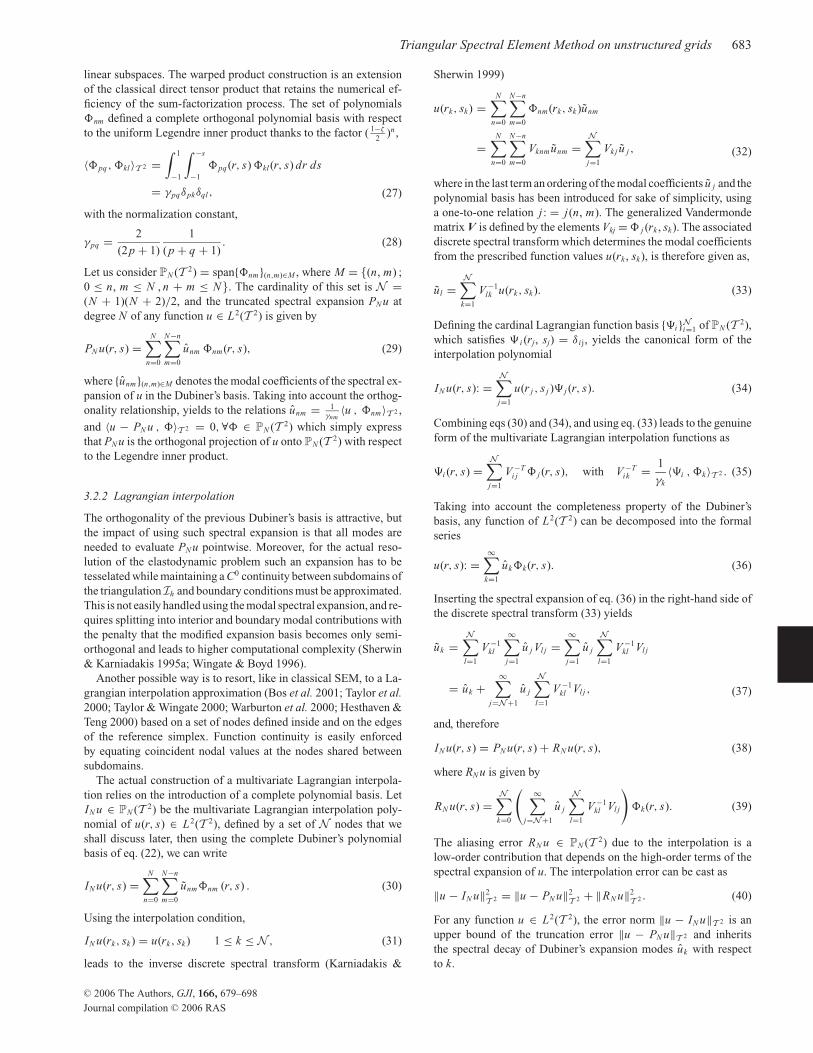
Figure 2. (Left) Schema of the homogeneous domain with bi-periodic
boundary conditions. Source and receiver locations are shown. (Right) De-
tail of structured meshes. Global interpolation points with polynomial order
of 5. Fekete points (•) used in this study, Gauss–Lobatto–Legendre points
(×) used in classical SEM. Note that both set of points coincide at element’s
edges.
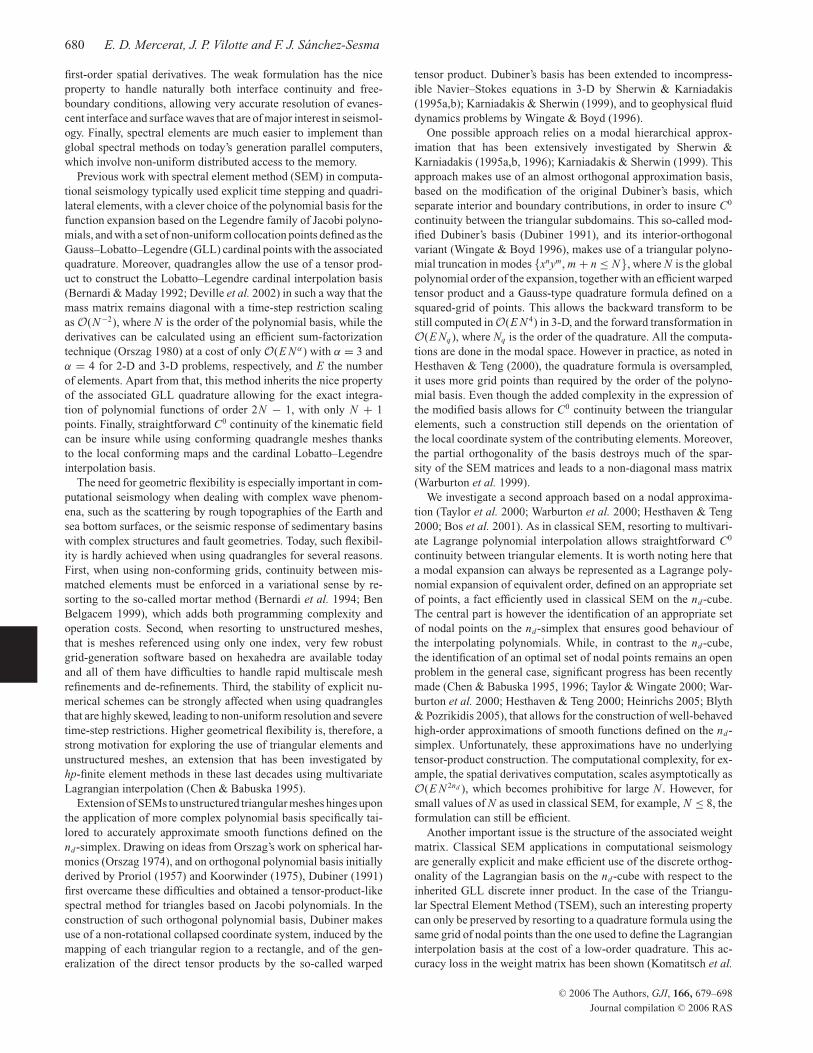
0 0.5 1 1.5 2time (s)
AnalytiqueResiduals*5 triangular elementsResiduals*5 quadrangular elements
AnalyticalResiduals*5 triangular elementsResiduals*5 quadrangular elements
Figure 3. Horizontal component of the displacement field at receiver 1.
Residuals between analytical and numerical solutions are amplified by a
factor of 5. The vertical component is exactly similar (not shown).
number of 40401 interpolation points. In Fig. 2 both set of interpo-
lation points are shown to coincide at the element edges. The number
of points per minimum wavelength λmin = Vs/ f max with f max = 2.5
f 0 is between 4 and 5, which is the accuracy lower limit when using
classical SEM (Seriani et al. 1992; Komatitsch & Vilotte 1998).
Bi-periodic boundary conditions are imposed to propagate waves
several times through the grid and a time step �t = 0.5 ms is used,
corresponding to a Courant number of 0.3. Simulations have been
performed on the triangular mesh and on the quadrangular mesh,
both up to 2 s total time (4000 time steps). Comparison of the hori-
zontal displacement predicted by the TSEM and the classical SEM
for the horizontal component at receiver 1 can be seen in Fig. 3.
Comparison with the analytical solution shows that both methods
perform well even for waves travelling several times through the
computational mesh, for example arrivals later than 0.5 s.
4.1.2 Unstructured triangulation
The main advantage of triangular elements is to resort to unstruc-
tured meshes for the discretization of complex geometries. In this
section we assess the performance of the TSEM when using an un-
structured mesh built with the help of the mesh generator Triangleof Shewchuk (1996). It is worth noting here that for homogeneous
media, this mesh generator does not seem to be optimal, for ex-
ample, it does not generate equilateral triangles within an homoge-
neous medium for bi-periodic boundary conditions. The numerical
example of the previous section is repeated here but now using a
unstructured mesh shown in Fig. 4. This mesh is composed of 3202
triangles and 40426 global grid points, when using polynomial or-
der of degree 5 for the interpolation within each triangular element
(quite similar to the 3200 elements and 40 401 global grid points
used in the structured case). Bi-periodic boundary conditions are
again imposed. Keeping the same source and time parameters as in
the structured case, leads to 5 points per minimum wavelength and a
Courant number of about 0.3. A snapshot of the displacement field
at t = 0.5 s is shown Fig. 4 where no S wave is observed even in the
case of such an unstructured mesh.
As in the previous example, the horizontal component of the
displacement field calculated by the TSEM using the unstructured
mesh is shown in Fig. 5 against the analytical solution. The result
is quite accurate and it compares well with both structured mesh
simulations shown in Fig. 3.
In a second test, both the consistent and the lumped mass TSEM
are compared when using the unstructured triangular mesh. The re-
sults are shown in Fig. 6 where only the first P arrivals are compared
to the analytical solution. The consistent TSEM formulation clearly
exhibits much better accuracy than the lumped mass formulation. A
C© 2006 The Authors, GJI, 166, 679–698
Journal compilation C© 2006 RAS
Triangular Spectral Element Method on unstructured grids 687
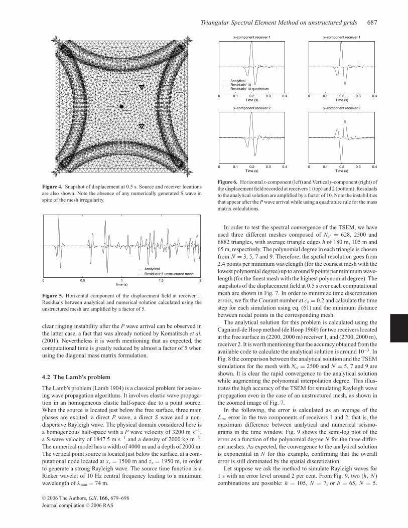
Figure 4. Snapshot of displacement at 0.5 s. Source and receiver locations
are also shown. Note the absence of any numerically generated S wave in
spite of the mesh irregularity.
0 0.5 1 1.5 2time (s)
AnalytiqueResiduals*5 unstructured mesh
Analytical
Residuals*5 unstructured mesh
Figure 5. Horizontal component of the displacement field at receiver 1.
Residuals between analytical and numerical solution calculated using the
unstructured mesh are amplified by a factor of 5.
clear ringing instability after the P wave arrival can be observed in
the latter case, a fact that was already noticed by Komatitsch et al.(2001). Nevertheless it is worth mentioning that as expected, the
computational time is greatly reduced by almost a factor of 5 when
using the diagonal mass matrix formulation.
4.2 The Lamb’s problem
The Lamb’s problem (Lamb 1904) is a classical problem for assess-
ing wave propagation algorithms. It involves elastic wave propaga-
tion in an homogeneous elastic half-space due to a point source.
When the source is located just below the free surface, three main
phases are excited: a direct P wave, a direct S wave and a non-
dispersive Rayleigh wave. The physical domain considered here is
a homogeneous half-space with a P wave velocity of 3200 m s−1,
a S wave velocity of 1847.5 m s−1 and a density of 2000 kg m−3.
The numerical model has a width of 4000 m and a depth of 2000 m.
The vertical point source is located just below the surface, at a com-
putational node located at xs = 1500 m and zs = 1950 m, in order
to generate a strong Rayleigh wave. The source time function is a
Ricker wavelet of 10 Hz central frequency leading to a minimum
wavelength of λmin = 74 m.
0 0.1 0.2 0.3 0.4
x–component receiver 1
Time (s)
AnalyticalResiduals*10Residuals*10 quadrature
0 0.1 0.2 0.3 0.4
y–component receiver 1
Time (s)
0 0.1 0.2 0.3 0.4
x–component receiver 2
Time (s)0 0.1 0.2 0.3 0.4
y–component receiver 2
Time (s)
Figure 6. Horizontal x-component (left) and Vertical y-component (right) of
the displacement field recorded at receivers 1 (top) and 2 (bottom). Residuals
to the analytical solution are amplified by a factor of 10. Note the instabilities
that appear after the P wave arrival while using a quadrature rule for the mass
matrix calculations.
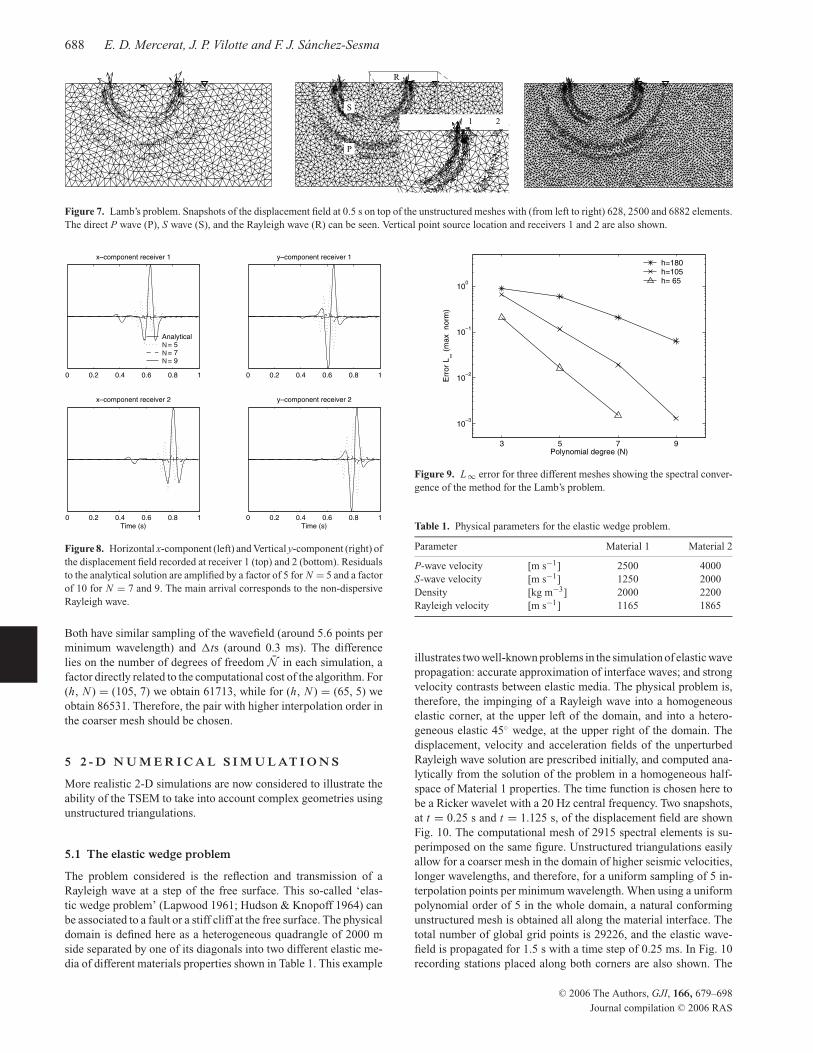
In order to test the spectral convergence of the TSEM, we have
used three different meshes composed of Nel = 628, 2500 and
6882 triangles, with average triangle edges h of 180 m, 105 m and
65 m, respectively. The polynomial degree in each triangle is chosen
from N = 3, 5, 7 and 9. Therefore, the spatial resolution goes from
2.4 points per minimum wavelength (for the coarsest mesh with the
lowest polynomial degree) up to around 9 points per minimum wave-
length (for the finest mesh with the highest polynomial degree). The
snapshots of the displacement field at 0.5 s over each computational
mesh are shown in Fig. 7. In order to minimize time discretization
errors, we fix the Courant number at ch = 0.2 and calculate the time
step for each simulation using eq. (61) and the minimum distance
between nodal points in the corresponding mesh.
The analytical solution for this problem is calculated using the
Cagniard-de Hoop method (de Hoop 1960) for two receivers located
at the free surface in (2200, 2000 m) receiver 1, and (2700, 2000 m),
receiver 2. It is worth mentioning that the accuracy obtained from the
available code to calculate the analytical solution is around 10−3. In
Fig. 8 the comparison between the analytical solution and the TSEM
simulations for the mesh with Nel = 2500 and N = 5, 7 and 9 are
shown. It is clear the rapid convergence to the analytical solution
while augmenting the polynomial interpolation degree. This illus-
trates the high accuracy of the TSEM for simulating Rayleigh wave
propagation even in the case of an unstructured mesh, as shown in
the zoomed image of Fig. 7.
In the following, the error is calculated as an average of the
L ∞ error in the two components of receivers 1 and 2, that is, the
maximum difference between analytical and numerical seismo-
grams in the time window. Fig. 9 shows the semi-log plot of the
error as a function of the polynomial degree N for the three differ-
ent meshes. As expected, the convergence to the analytical solution
is exponential in N for this example, confirming that the overall
error is still dominated by the spatial discretization.
Let suppose we ask the method to simulate Rayleigh waves for
1 s with an error level around 2 per cent. From Fig. 9, two (h, N )
combinations are possible: h = 105, N = 7, or h = 65, N = 5.
C© 2006 The Authors, GJI, 166, 679–698
Journal compilation C© 2006 RAS
688 E. D. Mercerat, J. P. Vilotte and F. J. Sanchez-Sesma
P
S
R
1 2
Figure 7. Lamb’s problem. Snapshots of the displacement field at 0.5 s on top of the unstructured meshes with (from left to right) 628, 2500 and 6882 elements.
The direct P wave (P), S wave (S), and the Rayleigh wave (R) can be seen. Vertical point source location and receivers 1 and 2 are also shown.
0 0.2 0.4 0.6 0.8 1
x–component receiver 1
Analyticalp = 5p = 7p = 9
0 0.2 0.4 0.6 0.8 1
y–component receiver 1
0 0.2 0.4 0.6 0.8 1
x–component receiver 2
Time (s)0 0.2 0.4 0.6 0.8 1
y–component receiver 2
Time (s)
N
NN
Figure 8. Horizontal x-component (left) and Vertical y-component (right) of
the displacement field recorded at receiver 1 (top) and 2 (bottom). Residuals
to the analytical solution are amplified by a factor of 5 for N = 5 and a factor
of 10 for N = 7 and 9. The main arrival corresponds to the non-dispersive
Rayleigh wave.
Both have similar sampling of the wavefield (around 5.6 points per
minimum wavelength) and �ts (around 0.3 ms). The difference
lies on the number of degrees of freedom N in each simulation, a
factor directly related to the computational cost of the algorithm. For
(h, N ) = (105, 7) we obtain 61713, while for (h, N ) = (65, 5) we
obtain 86531. Therefore, the pair with higher interpolation order in
the coarser mesh should be chosen.
5 2 - D N U M E R I C A L S I M U L AT I O N S
More realistic 2-D simulations are now considered to illustrate the
ability of the TSEM to take into account complex geometries using
unstructured triangulations.
5.1 The elastic wedge problem
The problem considered is the reflection and transmission of a
Rayleigh wave at a step of the free surface. This so-called ‘elas-
tic wedge problem’ (Lapwood 1961; Hudson & Knopoff 1964) can
be associated to a fault or a stiff cliff at the free surface. The physical
domain is defined here as a heterogeneous quadrangle of 2000 m
side separated by one of its diagonals into two different elastic me-
dia of different materials properties shown in Table 1. This example
3 5 7 9
10–3
10–2
10–1
100
Polynomial degree (N)E
rro
r L
∞ (
ma
xn
orm
)
h=180h=105h= 65
Figure 9. L ∞ error for three different meshes showing the spectral conver-
gence of the method for the Lamb’s problem.
Table 1. Physical parameters for the elastic wedge problem.
Parameter Material 1 Material 2
P-wave velocity [m s−1] 2500 4000
S-wave velocity [m s−1] 1250 2000
Density [kg m−3] 2000 2200
Rayleigh velocity [m s−1] 1165 1865
illustrates two well-known problems in the simulation of elastic wave
propagation: accurate approximation of interface waves; and strong
velocity contrasts between elastic media. The physical problem is,
therefore, the impinging of a Rayleigh wave into a homogeneous
elastic corner, at the upper left of the domain, and into a hetero-
geneous elastic 45◦ wedge, at the upper right of the domain. The
displacement, velocity and acceleration fields of the unperturbed
Rayleigh wave solution are prescribed initially, and computed ana-
lytically from the solution of the problem in a homogeneous half-
space of Material 1 properties. The time function is chosen here to
be a Ricker wavelet with a 20 Hz central frequency. Two snapshots,
at t = 0.25 s and t = 1.125 s, of the displacement field are shown
Fig. 10. The computational mesh of 2915 spectral elements is su-
perimposed on the same figure. Unstructured triangulations easily
allow for a coarser mesh in the domain of higher seismic velocities,
longer wavelengths, and therefore, for a uniform sampling of 5 in-
terpolation points per minimum wavelength. When using a uniform
polynomial order of 5 in the whole domain, a natural conforming
unstructured mesh is obtained all along the material interface. The
total number of global grid points is 29226, and the elastic wave-
field is propagated for 1.5 s with a time step of 0.25 ms. In Fig. 10
recording stations placed along both corners are also shown. The
C© 2006 The Authors, GJI, 166, 679–698
Journal compilation C© 2006 RAS
Triangular Spectral Element Method on unstructured grids 689
Rayleigh wave
Receivers Receivers5175
101
1 25
50
Rt
Rr
P
Rr
Rt
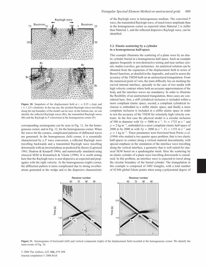
Figure 10. Snapshots of the displacement field at t = 0.25 s (top) and
t = 1.125 s (bottom). In the top one, the incident Rayleigh waves travelling
along the top boundary of the model can be seen. In the bottom one, we can
identify the reflected Rayleigh waves (Rr), the transmitted Rayleigh waves
(Rt) and the Rayleigh to P conversion at the homogeneous corner (P).
corresponding seismograms can be seen in Fig. 11, for the homo-
geneous corner, and in Fig. 12, for the heterogeneous corner. When
the waves hit the corners, complicated patterns of diffracted waves
are generated. In the homogeneous (left) corner, it is essentially
characterized by a P wave conversion, a reflected Rayleigh wave
travelling backwards and a transmitted Rayleigh wave travelling
downwards with an inverted phase as predicted by theory (Lapwood
1961; Hudson & Knopoff 1964), and numerically simulated using
classical SEM in Komatitsch & Vilotte (1998). It is worth noting
here that the Rayleigh wave is non-dispersive as expected and prop-
agates with the right velocity. At the heterogeneous (right) corner,
the diffraction pattern is more complicated due to strong reverber-
ations generated at the wedge and to the dispersive characteristic
0
0.5
1.0
1.5
60 70 80 900
0.5
1.0
1.5
60 70 80 90
Tim
e[s
]
Tim
e[s
]
Receiver number Receiver number
Rt RtRr RrP
Figure 11. Seismograms of horizontal (left) and vertical component (right) of the displacement field recorded at the homogeneous corner. We identify the
main events of Fig. 10.
of the Rayleigh wave in heterogeneous medium. The converted Pwave, the transmitted Rayleigh wave, of much lower amplitude than
in the homogeneous corner as expected when Material 2 is stiffer
than Material 1, and the reflected dispersive Rayleigh wave, can be
identified.
5.2 Elastic scattering by a cylinder
in a homogeneous half-space
This example illustrates the scattering of a plane wave by an elas-
tic cylinder buried in a homogeneous half-space. Such an example
appears frequently in non-destructive testing and near surface seis-
mic studies (cavities, gas inclusions). An analytical solution can be
obtained from the expansion of the displacement field in series of
Bessel functions, as detailed in the Appendix, and used to assess the
accuracy of the TSEM built on an unstructured triangulation. From
the numerical point of view, the main difficulty lies on meshing the
curved internal interface, specially in the case of two media with
high velocity contrast where both an accurate approximation of the
body and the interface waves are mandatory. In order to illustrate
the flexibility of an unstructured triangulation, three cases are con-
sidered here: first, a stiff cylindrical inclusion is included within a
more compliant elastic space; second, a compliant cylindrical in-
clusion is embedded in a stiffer elastic space; and finally a more
compliant inclusion is included in a stiffer elastic space in order
to test the accuracy of the TSEM for extremely high velocity con-
trasts. In the first case the physical model is a circular inclusion
of 500 m diameter with Vp = 3000 m s−1, Vs = 1732 m s−1 and
ρ = 2 kg m−3, embedded in a more compliant elastic half-space of
2000 m by 2000 m with Vp = 2000 m s−1, Vs = 1155 m s−1 and
ρ = 1 kg m−3. These parameters were borrowed from Priolo et al.(1994) who studied a two quarter space problem, that is two elastic
half-spaces in contact along a vertical material discontinuity, with
special emphasis in the simulation of the interface wave travelling
along the vertical interface, a geometry that is well suited for clas-
sical SEM based on a quadrangular mesh. Here the scattering by
an elastic cylinder of a plane wave travelling downwards is consid-
ered. In this problem, an interface wave is expected to travel along
the circular boundary of the buried cylinder. The triangulation in
this example is composed of 3402 triangles, with a total number
of 42 846 global Fekete points when using a polynomial degree of
C© 2006 The Authors, GJI, 166, 679–698
Journal compilation C© 2006 RAS
690 E. D. Mercerat, J. P. Vilotte and F. J. Sanchez-Sesma
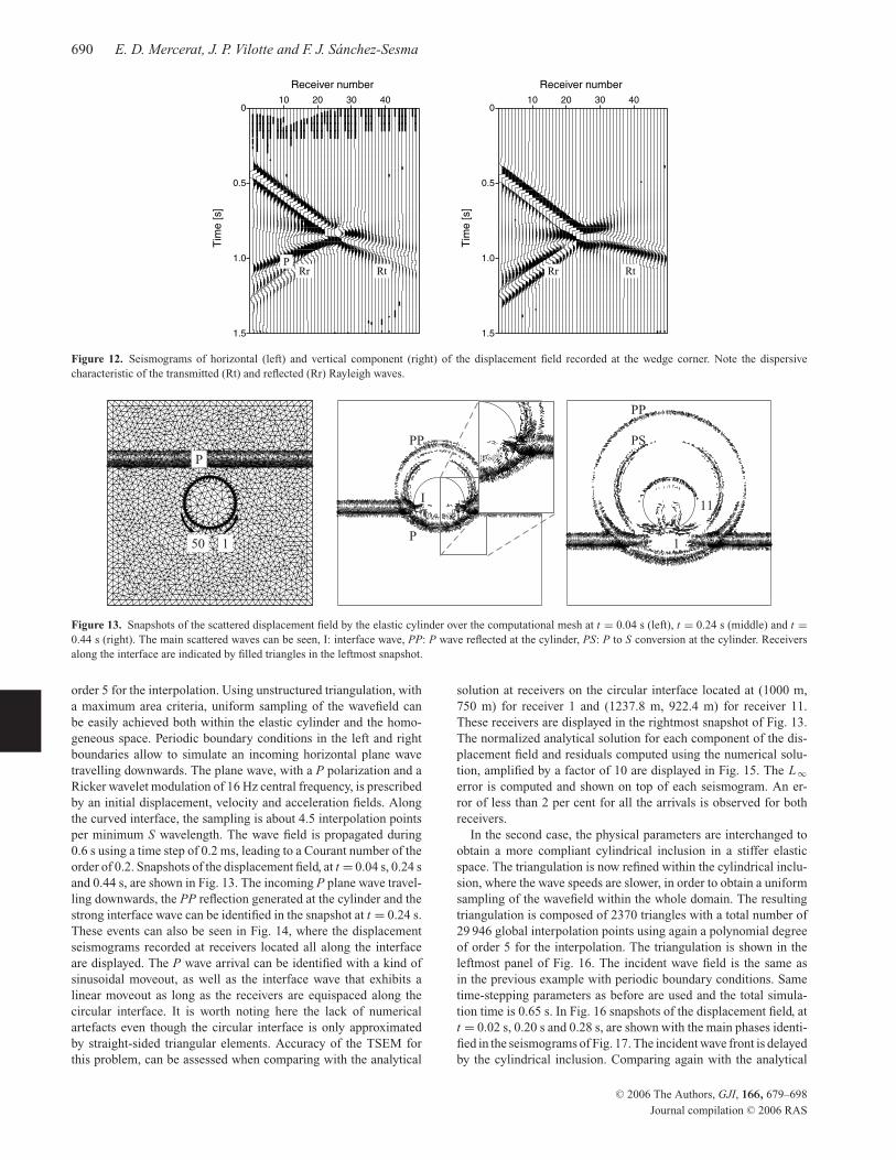
0
0.5
1.0
1.5
10 20 30 400
0.5
1.0
1.5
10 20 30 40
Tim
e[s
]
Tim
e[s
]
Receiver number Receiver number
Rt RtRr RrP
Figure 12. Seismograms of horizontal (left) and vertical component (right) of the displacement field recorded at the wedge corner. Note the dispersive
characteristic of the transmitted (Rt) and reflected (Rr) Rayleigh waves.
P
I
P
PP
PP
PS
150 1
11
Figure 13. Snapshots of the scattered displacement field by the elastic cylinder over the computational mesh at t = 0.04 s (left), t = 0.24 s (middle) and t =0.44 s (right). The main scattered waves can be seen, I: interface wave, PP: P wave reflected at the cylinder, PS: P to S conversion at the cylinder. Receivers
along the interface are indicated by filled triangles in the leftmost snapshot.
order 5 for the interpolation. Using unstructured triangulation, with
a maximum area criteria, uniform sampling of the wavefield can
be easily achieved both within the elastic cylinder and the homo-
geneous space. Periodic boundary conditions in the left and right
boundaries allow to simulate an incoming horizontal plane wave
travelling downwards. The plane wave, with a P polarization and a
Ricker wavelet modulation of 16 Hz central frequency, is prescribed
by an initial displacement, velocity and acceleration fields. Along
the curved interface, the sampling is about 4.5 interpolation points
per minimum S wavelength. The wave field is propagated during
0.6 s using a time step of 0.2 ms, leading to a Courant number of the
order of 0.2. Snapshots of the displacement field, at t = 0.04 s, 0.24 s
and 0.44 s, are shown in Fig. 13. The incoming P plane wave travel-
ling downwards, the PP reflection generated at the cylinder and the
strong interface wave can be identified in the snapshot at t = 0.24 s.
These events can also be seen in Fig. 14, where the displacement
seismograms recorded at receivers located all along the interface
are displayed. The P wave arrival can be identified with a kind of
sinusoidal moveout, as well as the interface wave that exhibits a
linear moveout as long as the receivers are equispaced along the
circular interface. It is worth noting here the lack of numerical
artefacts even though the circular interface is only approximated
by straight-sided triangular elements. Accuracy of the TSEM for
this problem, can be assessed when comparing with the analytical
solution at receivers on the circular interface located at (1000 m,
750 m) for receiver 1 and (1237.8 m, 922.4 m) for receiver 11.
These receivers are displayed in the rightmost snapshot of Fig. 13.
The normalized analytical solution for each component of the dis-
placement field and residuals computed using the numerical solu-
tion, amplified by a factor of 10 are displayed in Fig. 15. The L ∞error is computed and shown on top of each seismogram. An er-
ror of less than 2 per cent for all the arrivals is observed for both
receivers.
In the second case, the physical parameters are interchanged to
obtain a more compliant cylindrical inclusion in a stiffer elastic
space. The triangulation is now refined within the cylindrical inclu-
sion, where the wave speeds are slower, in order to obtain a uniform
sampling of the wavefield within the whole domain. The resulting
triangulation is composed of 2370 triangles with a total number of
29 946 global interpolation points using again a polynomial degree
of order 5 for the interpolation. The triangulation is shown in the
leftmost panel of Fig. 16. The incident wave field is the same as
in the previous example with periodic boundary conditions. Same
time-stepping parameters as before are used and the total simula-
tion time is 0.65 s. In Fig. 16 snapshots of the displacement field, at
t = 0.02 s, 0.20 s and 0.28 s, are shown with the main phases identi-
fied in the seismograms of Fig. 17. The incident wave front is delayed
by the cylindrical inclusion. Comparing again with the analytical
C© 2006 The Authors, GJI, 166, 679–698
Journal compilation C© 2006 RAS

Triangular Spectral Element Method on unstructured grids 691
0
0.2
0.4T
ime (
s)
10 20 30 40 50Receiver number
0
0.2
0.4
Tim
e (
s)
10 20 30 40 50Receiver number
P
I
P
I
Figure 14. Seismograms of horizontal (left) and vertical component (right) of the displacement field recorded at the receivers located all along the circular
interface (stiff inclusion). P: direct P wave arrival, St: Stoneley wave travelling along the circular interface.
0 0.2 0.4 0.6
x–comp rec 1 L∞ = 0.0013995
Time [s]
AnalyticalResiduals*10
0 0.2 0.4 0.6
z–comp rec 1 L∞ = 0.015648
Time [s]0 0.2 0.4 0.6
x–comp rec 11 L∞ = 0.012856
Time [s]0 0.2 0.4 0.6
z–comp rec 11 L = 0.011436
Time [s]
Figure 15. Horizontal x-component and vertical z-component of the displacement field recorded at receivers 1 and 11 (stiff inclusion). Residuals are amplified
by a factor of 10. As expected, there is no energy in the horizontal component of receiver 1 placed on the cylinder axis. The arrival around 0.3 s at receiver 11
corresponds to the interface wave.
Figure 16. Snapshots of the scattered displacement field by the elastic cylinder over the computational mesh at t = 0.02 s (left), t = 0.20 s (middle) and t =0.28 s (right). The main scattered waves can be seen, I: interface wave, PP: P wave reflected at the cylinder, PS: P to S conversion at the cylinder. Receivers
along the interface are indicated by filled triangles in the leftmost snapshot.
solution at the same receivers used for the first case, Fig. 18, en-
sures an error of less than 2 per cent between the analytical and
numerical solutions.
In the third case, a much higher velocity contrast between the com-
pliant cylindrical inclusion and the surrounding space is created by
using Vp = 4000 m s−1, Vs = 2310 m s−1 and ρ = 2 kg m−3 for the
elastic space and Vp = 1400 m s−1, Vs = 600 m s−1 and ρ = 1 kg m−3
for the inclusion. The incident wavefield is the same as in the previ-
ous examples with periodic boundary conditions. In order to keep
a similar Courant number of 0.2, the time step must be reduced to
0.112 ms for this simulation due to the strong mesh refinement in the
cylindrical inclusion. In Fig. 19 snapshots of the displacement field,
at t = 0.0 s, 0.2 s and 0.3 s, are shown with the main phases identi-
fied in the seismograms of Fig. 20. It is interesting to note in Fig. 21
similar error levels as in the previous case (less than 2 per cent),
showing the robustness of the method to deal with such strong
velocity contrast within the elastic medium.
5.3 Elastic half-space with free-surface
and interface topographies
The flexibility of an unstructured triangulation for wave propagation
simulation can be illustrated when considering wave propagation in
a layered 2-D elastic domain with arbitrary topography of the free
C© 2006 The Authors, GJI, 166, 679–698
Journal compilation C© 2006 RAS
692 E. D. Mercerat, J. P. Vilotte and F. J. Sanchez-Sesma
0
0.2
0.4
0.6
Tim
e (
s)
10 20 30 40 50Receiver number
0
0.2
0.4
0.6
Tim
e (
s)
10 20 30 40 50Receiver number
I I
Figure 17. Seismograms of horizontal (left) and vertical component (right) of the displacement field recorded at the receivers located all along the circular
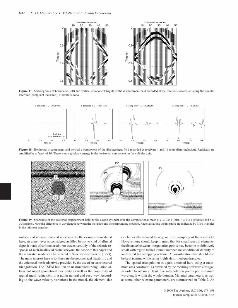
interface (compliant inclusion). I: interface wave.
0 0.2 0.4 0.6
x–comp rec 1 L∞ = 0.001301
Time [s]
AnalyticalResiduals*10
0 0.2 0.4 0.6
z–comp rec 1 L∞ = 0.017576
Time [s]0 0.2 0.4 0.6
x–comp rec 11 L∞ = 0.013969
Time [s]0 0.2 0.4 0.6
z–comp rec 11 L∞ = 0.017051
Time [s]
Figure 18. Horizontal x-component and vertical z-component of the displacement field recorded at receivers 1 and 11 (compliant inclusion). Residuals are
amplified by a factor of 10. There is no significant energy in the horizontal component on the cylinder axis.
Figure 19. Snapshots of the scattered displacement field by the elastic cylinder over the computational mesh at t = 0.0 s (left), t = 0.2 s (middle) and t =0.3 s (right). Note the difference in wavelength between the inclusion and the surrounding medium. Receivers along the interface are indicated by filled triangles
in the leftmost snapshot.
surface and internal material interfaces. In the example considered
here, an upper layer is considered as filled by some kind of alluvial
deposit made of soft materials. An extensive study of the seismic re-
sponse of such an alluvial basin is beyond the scope of this paper and
the interested reader can be referred to Sanchez-Sesma et al. (1993).
The main interest here is to illustrate the geometrical flexibility and
the enhanced mesh adaptivity provided by the use of an unstructured
triangulation. The TSEM built on an unstructured triangulation al-
lows enhanced geometrical flexibility as well as the possibility of
spatial mesh refinement in a rather natural and easy way. Accord-
ing to the wave velocity variations in the model, the element size
can be locally reduced to keep uniform sampling of the wavefield.
However, one should keep in mind that for small spectral elements,
the distance between interpolation points may become prohibitively
small with regard to the Courant number and conditional stability of
an explicit time-stepping scheme. A consideration that should also
be kept in mind while using highly deformed quadrangles.
The spatial triangulation is again obtained here using a maxi-
mum area constraint, as provided by the meshing software Triangle,
in order to obtain at least five interpolation points per minimum
wavelength within the whole domain. Material parameters, as well
as some other relevant parameters, are summarized in Table 2. An
C© 2006 The Authors, GJI, 166, 679–698
Journal compilation C© 2006 RAS
Triangular Spectral Element Method on unstructured grids 693
0
0.2
0.4
0.6
Tim
e (
s)
10 20 30 40 50Receiver number
0
0.2
0.4
0.6
Tim
e (
s)
10 20 30 40 50Receiver number
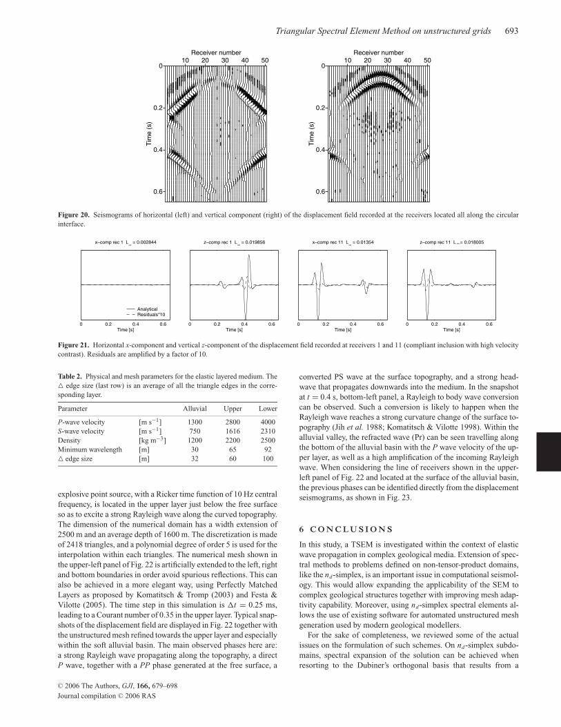
Figure 20. Seismograms of horizontal (left) and vertical component (right) of the displacement field recorded at the receivers located all along the circular
interface.
0 0.2 0.4 0.6
x–comp rec 1 L∞ = 0.002844
Time [s]
AnalyticalResiduals*10
0 0.2 0.4 0.6
z–comp rec 1 L∞ = 0.019856
Time [s]0 0.2 0.4 0.6
x–comp rec 11 L∞ = 0.01354
Time [s]0 0.2 0.4 0.6
z–comp rec 11 L = 0.018005
Time [s]
∞
Figure 21. Horizontal x-component and vertical z-component of the displacement field recorded at receivers 1 and 11 (compliant inclusion with high velocity
contrast). Residuals are amplified by a factor of 10.
Table 2. Physical and mesh parameters for the elastic layered medium. The
� edge size (last row) is an average of all the triangle edges in the corre-
sponding layer.
Parameter Alluvial Upper Lower
P-wave velocity [m s−1] 1300 2800 4000
S-wave velocity [m s−1] 750 1616 2310
Density [kg m−3] 1200 2200 2500
Minimum wavelength [m] 30 65 92
� edge size [m] 32 60 100
explosive point source, with a Ricker time function of 10 Hz central
frequency, is located in the upper layer just below the free surface
so as to excite a strong Rayleigh wave along the curved topography.
The dimension of the numerical domain has a width extension of
2500 m and an average depth of 1600 m. The discretization is made
of 2418 triangles, and a polynomial degree of order 5 is used for the
interpolation within each triangles. The numerical mesh shown in
the upper-left panel of Fig. 22 is artificially extended to the left, right
and bottom boundaries in order avoid spurious reflections. This can
also be achieved in a more elegant way, using Perfectly Matched
Layers as proposed by Komatitsch & Tromp (2003) and Festa &
Vilotte (2005). The time step in this simulation is �t = 0.25 ms,
leading to a Courant number of 0.35 in the upper layer. Typical snap-
shots of the displacement field are displayed in Fig. 22 together with
the unstructured mesh refined towards the upper layer and especially
within the soft alluvial basin. The main observed phases here are:
a strong Rayleigh wave propagating along the topography, a direct
P wave, together with a PP phase generated at the free surface, a
converted PS wave at the surface topography, and a strong head-
wave that propagates downwards into the medium. In the snapshot
at t = 0.4 s, bottom-left panel, a Rayleigh to body wave conversion
can be observed. Such a conversion is likely to happen when the
Rayleigh wave reaches a strong curvature change of the surface to-
pography (Jih et al. 1988; Komatitsch & Vilotte 1998). Within the
alluvial valley, the refracted wave (Pr) can be seen travelling along
the bottom of the alluvial basin with the P wave velocity of the up-
per layer, as well as a high amplification of the incoming Rayleigh
wave. When considering the line of receivers shown in the upper-
left panel of Fig. 22 and located at the surface of the alluvial basin,
the previous phases can be identified directly from the displacement
seismograms, as shown in Fig. 23.
6 C O N C L U S I O N S
In this study, a TSEM is investigated within the context of elastic
wave propagation in complex geological media. Extension of spec-
tral methods to problems defined on non-tensor-product domains,
like the nd-simplex, is an important issue in computational seismol-
ogy. This would allow expanding the applicability of the SEM to
complex geological structures together with improving mesh adap-
tivity capability. Moreover, using nd-simplex spectral elements al-
lows the use of existing software for automated unstructured mesh
generation used by modern geological modellers.
For the sake of completeness, we reviewed some of the actual
issues on the formulation of such schemes. On nd-simplex subdo-
mains, spectral expansion of the solution can be achieved when
resorting to the Dubiner’s orthogonal basis that results from a
C© 2006 The Authors, GJI, 166, 679–698
Journal compilation C© 2006 RAS

694 E. D. Mercerat, J. P. Vilotte and F. J. Sanchez-Sesma
1 100Receivers
P
PS
R
RtoS
PP
Pr
Figure 22. Snapshot of the displacement field in the layered elastic half-space at 0.2 s, 0.3 s, 0.4 s, 0.5 s (from top left to bottom right). Some main wave fronts
are identified: P direct P wave (P), converted P to S at the free surface (PS), Rayleigh wave (R), Rayleigh to S wave conversion (RtoS), refracted P wave (Pr).
The numerical mesh, the source and the receiver line location can be seen in the top-left snapshot.
0
0.2
0.4
0.6
0.8
10 30 50 70 900
0.2
0.4
0.6
0.8
10 30 50 70 90
Tim
e[s
]
Tim
e[s
]
rebmunrevieceRrebmunrevieceR
P
Pr
R
RtoP
PtoR
Figure 23. Seismograms of the horizontal (left) and vertical component (right) of the displacement field recorded at the top of the alluvial valley. Some main
events are identified: direct P wave (P), refracted P wave at the bottom of the alluvial valley (Pr), Rayleigh wave (R), Rayleigh to body wave conversion (RtoP)
and P to Rayleigh conversion (PtoR) at the valley’s tip.
warped tensor product of Jacobi polynomials associated with a local
collapsed coordinate system. Such a construction can be seen as a
generalization of the classical tensor product construction in use
with classical SEM built on tensor product domains. This orthogo-
nal polynomial basis can be shown to be the solution of a Sturm–
Liouville eigenvalue problem defined on the reference simplex, and
therefore, to achieve spectral accuracy. Based on this orthogonal
basis, a TSEM can be constructed by resorting, as in classical SEM,
to a multivariate Lagrangian interpolation designed to enforce in
a natural way the C0 continuity requirement between subdomains
of the triangulation. Today, even though no optimal set of points
is known for interpolation on a non-tensor product-domain, such a
multivariate Lagrangian interpolation can be built based on the set
of Fekete points that are shown to endow good interpolation prop-
erties and to maximize the number of points on the boundary of the
subdomains. In these boundaries, Fekete points turn out to coincide
with the classical GLL points used in classical SEM. However, in
contrast with the GLL set of points defined on tensor product do-
mains, Fekete points do not define an optimal quadrature formula in
the sense that the associated Newton–Cotes quadrature formula only
C© 2006 The Authors, GJI, 166, 679–698
Journal compilation C© 2006 RAS
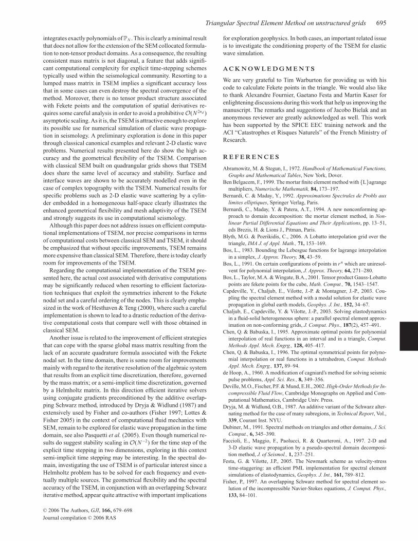
Triangular Spectral Element Method on unstructured grids 695
integrates exactly polynomials of PN . This is clearly a minimal result
that does not allow for the extension of the SEM collocated formula-
tion to non-tensor product domains. As a consequence, the resulting
consistent mass matrix is not diagonal, a feature that adds signifi-
cant computational complexity for explicit time-stepping schemes
typically used within the seismological community. Resorting to a
lumped mass matrix in TSEM implies a significant accuracy loss
that in some cases can even destroy the spectral convergence of the
method. Moreover, there is no tensor product structure associated
with Fekete points and the computation of spatial derivatives re-
quires some careful analysis in order to avoid a prohibitive O(N 2nd )
asymptotic scaling. As it is, the TSEM is attractive enough to explore
its possible use for numerical simulation of elastic wave propaga-
tion in seismology. A preliminary exploration is done in this paper
through classical canonical examples and relevant 2-D elastic wave
problems. Numerical results presented here do show the high ac-
curacy and the geometrical flexibility of the TSEM. Comparison
with classical SEM built on quadrangular grids shows that TSEM
does share the same level of accuracy and stability. Surface and
interface waves are shown to be accurately modelled even in the
case of complex topography with the TSEM. Numerical results for
specific problems such as 2-D elastic wave scattering by a cylin-
der embedded in a homogeneous half-space clearly illustrates the
enhanced geometrical flexibility and mesh adaptivity of the TSEM
and strongly suggests its use in computational seismology.
Although this paper does not address issues on efficient computa-
tional implementations of TSEM, nor precise comparisons in terms
of computational costs between classical SEM and TSEM, it should
be emphasized that without specific improvements, TSEM remains
more expensive than classical SEM. Therefore, there is today clearly
room for improvements of the TSEM.
Regarding the computational implementation of the TSEM pre-
sented here, the actual cost associated with derivative computations
may be significantly reduced when resorting to efficient factoriza-
tion techniques that exploit the symmetries inherent to the Fekete
nodal set and a careful ordering of the nodes. This is clearly empha-
sized in the work of Hesthaven & Teng (2000), where such a careful
implementation is shown to lead to a drastic reduction of the deriva-
tive computational costs that compare well with those obtained in
classical SEM.
Another issue is related to the improvement of efficient strategies
that can cope with the sparse global mass matrix resulting from the
lack of an accurate quadrature formula associated with the Fekete
nodal set. In the time domain, there is some room for improvements
mainly with regard to the iterative resolution of the algebraic system
that results from an explicit time discretization, therefore, governed
by the mass matrix; or a semi-implicit time discretization, governed
by a Helmholtz matrix. In this direction efficient iterative solvers
using conjugate gradients preconditioned by the additive overlap-
ping Schwarz method, introduced by Dryja & Widlund (1987) and
extensively used by Fisher and co-authors (Fisher 1997; Lottes &
Fisher 2005) in the context of computational fluid mechanics with
SEM, remain to be explored for elastic wave propagation in the time
domain, see also Pasquetti et al. (2005). Even though numerical re-
sults do suggest stability scaling in O(N−2) for the time step of the
explicit time stepping in two dimensions, exploring in this context
semi-implicit time stepping may be interesting. In the spectral do-
main, investigating the use of TSEM is of particular interest since a
Helmholtz problem has to be solved for each frequency and even-
tually multiple sources. The geometrical flexibility and the spectral
accuracy of the TSEM, in conjunction with an overlapping Schwarz
iterative method, appear quite attractive with important implications
for exploration geophysics. In both cases, an important related issue
is to investigate the conditioning property of the TSEM for elastic
wave simulation.
A C K N O W L E D G M E N T S
We are very grateful to Tim Warburton for providing us with his
code to calculate Fekete points in the triangle. We would also like
to thank Alexandre Fournier, Gaetano Festa and Martin Kaser for
enlightening discussions during this work that help us improving the
manuscript. The remarks and suggestions of Jacobo Bielak and an
anonymous reviewer are greatly acknowledged as well. This work
has been supported by the SPICE EEC training network and the
ACI “Catastrophes et Risques Naturels” of the French Ministry of
Research.
R E F E R E N C E S
Abramowitz, M. & Stegun, I., 1972. Handbook of Mathematical Functions,Graphs and Mathematical Tables, New York, Dover.
Ben Belgacem, F., 1999. The mortar finite element method with {L}agrange
multipliers, Numerische Mathematik, 84, 173–197.
Bernardi, C. & Maday, Y., 1992. Approximations Spectrales de Probls auxlimites elliptiques, Springer Verlag, Paris.
Bernardi, C., Maday, Y. & Patera, A.T., 1994. A new nonconforming ap-
proach to domain decomposition: the mortar element method, in Non-linear Partial Differential Equations and Their Applications, pp. 13–51,
eds Brezis, H. & Lions J., Pitman, Paris.
Blyth, M.G. & Pozrikidis, C., 2006. A Lobatto interpolation grid over the
triangle, IMA J. of Appl. Math., 71, 153–169.
Bos, L., 1983. Bounding the Lebesgue functions for lagrange interpolation
in a simplex, J. Approx. Theory, 38, 43–59.
Bos, L., 1991. On certain configurations of points in rn which are uniresol-
vent for polynomial interpolation, J. Approx. Theory, 64, 271–280.
Bos, L., Taylor, M.A. & Wingate, B.A., 2001. Tensor product Gauss-Lobatto
points are fekete points for the cube, Math. Comput., 70, 1543–1547.
Capdeville, Y., Chaljub, E., Vilotte, J.-P. & Montagner, J.-P., 2003. Cou-
pling the spectral element method with a modal solution for elastic wave
propagation in global earth models, Geophys. J. Int., 152, 34–67.
Chaljub, E., Capdeville, Y. & Vilotte, J.-P., 2003. Solving elastodynamics
in a fluid-solid heterogeneous sphere: a parallel spectral element approx-
imation on non-conforming grids, J. Comput. Phys., 187(2), 457–491.
Chen, Q. & Babuska, I., 1995. Approximate optimal points for polynomial
interpolation of real functions in an interval and in a triangle, Comput.Methods Appl. Mech. Engrg., 128, 405–417.
Chen, Q. & Babuska, I., 1996. The optimal symmetrical points for polyno-
mial interpolation or real functions in a tetrahedron, Comput. MethodsAppl. Mech. Engrg., 137, 89–94.
de Hoop, A., 1960. A modification of cagniard’s method for solving seismic
pulse problems, Appl. Sci. Res., 8, 349–356.
Deville, M.O., Fischer, P.F. & Mund, E.H., 2002. High-Order Methods for In-compressible Fluid Flow, Cambridge Monographs on Applied and Com-
putational Mathematics, Cambridge Univ. Press.
Dryja, M. & Widlund, O.B., 1987. An additive variant of the Schwarz alter-
nating method for the case of many subregions, in Technical Report, Vol.,
339, Courant Inst. NYU.
Dubiner, M., 1991. Spectral methods on triangles and other domains, J. Sci.Comput., 6, 345–390.
Faccioli, E., Maggio, F., Paolucci, R. & Quarteroni, A., 1997. 2-D and
3-D elastic wave propagation by a pseudo-spectral domain decomposi-
tion method, J. of Seismol., 1, 237–251.
Festa, G. & Vilotte, J.P., 2005. The Newmark scheme as velocity-stress
time-staggering: an efficient PML implementation for spectral element
simulations of elastodynamics, Geophys. J. Int., 161, 789–812.
Fisher, P., 1997. An overlapping Schwarz method for spectral element so-
lution of the incompressible Navier-Stokes equations, J. Comput. Phys.,133, 84–101.
C© 2006 The Authors, GJI, 166, 679–698
Journal compilation C© 2006 RAS
696 E. D. Mercerat, J. P. Vilotte and F. J. Sanchez-Sesma
Giraldo, F.X. & Warburton, T., 2005. A nodal triangle based spectral element
method for the shallow water equations on the sphere, J. Comput. Phys.,207, 129–150.
Gottlieb, D. & Orszag, S.A., 1977. Numerical Analysis of Spectral Methods:Theory and Applications, SIAM-CMBS.
Heinrichs, W., 2005. Improved Lebesgue constants in the triangle, J. Comput.Phys., 207, 625–638.
Hesthaven, J.S., 1998. From electrostatics to almost optimal nodal sets for
polynomial interpolation in a simplex, SIAM J. Num. Anal., 35(2), 655–
676.
Hesthaven, J.S. & Teng, C.H., 2000. Stable spectral methods on tetrahedral
elements, SIAM J. Sci. Comput., 21(6), 2352–2380.
Hudson, J.A. & Knopoff, L., 1964. Transmission and reflection of a surface
wave at a corner, part2: Rayleigh waves (theoretical), J. geophys. Res., 69,281–289.
Hughes, T., 1987. The Finite Element Method, Linear Static and DynamicFinite Element Analysis, Prentice Hall International, Englewood Cliffs,
New Jersey.
Jih, R., McLaughlin, K. & Der, Z., 1988. Free-boundary conditions of ar-
bitrary polygonal topography in a two-dimensional explicit elastic finite-
difference scheme, Geophysics, 53(8), 1045–1055.
Jing, C. & Truell, R., 1956. Scattering of a plan longitudinal wave by a
spherical obstacle in an isotropically elastic solid, J. Appl. Phys., 27, 1086–
1097.
Karniadakis, G. & Sherwin, S., 1999. Spectral/hp Element Methods for Con-tinuum Fluid Dynamics, Cambridge University Press, Cambridge.
Komatitsch, D. & Tromp, J., 1999. Introduction to the spectral-element met-
hod for 3-D seismic wave propagation, Geophys. J. Int., 139, 806–822.
Komatitsch, D. & Tromp, J., 2003. A Perfectly Matched Layer absorbing
boundary condition for the second-order seismic wave equation, Geophys.J. Int., 154, 146–153.
Komatitsch, D. & Vilotte, J.P., 1998. The spectral-element method: an ef-
ficient tool to simulate the seismic response of 2-D and 3-D geological
structures, Bull. seism. Soc. Am., 88(2), 368–392.
Komatitsch, D., Vilotte, J.P., Vai, R., Castillo-Covarrubias, J.M. & Sanchez-
Sesma, F.J., 1999. The Spectral Element method for elastic wave equa-
tions: application to 2-D and 3-D seismic problems, Int. J. Numer. Meth.Engng., 45, 1139–1164.
Komatitsch, D., Barnes, C. & Tromp, J., 2000. Wave propagation near a fluid-
solid interface: a spectral element approach, Geophysics, 65(2), 623–631.
Komatitsch, D., Martin, R., Tromp, J., Taylor, M.A. & Wingate, B.A., 2001.
Wave propagation in 2-D elastic media using a spectral element method
with triangles and quadrangles, J. Comput. Acoust., 9(2), 703–718.
Komatitsch, D., Liu, Q., Tromp, J., Suss, P., Stidham, C. & Shaw, J.H., 2004.
Simulations of strong ground motion in the Los Angeles Basin based upon
the spectral-element method, Bull. seism. Soc. Am., 99, 187–206.
Koorwinder, T., 1975. Two-variable analogues of the classical orthogonal
polynomials, in Theory and applications of special functions, pp. 435–
495, ed, Askey, R.A., Academic Press.
Lamb, H., 1904. On the propagation of tremors over the surface of an elastic
solid, Phil. Trans. R. Soc. Lond, Ser., A., 203, 1–42.
Lapwood, E.R., 1961. The transition of a Rayleigh pulse round a corner,
Geophys. J., 4, 174–196.
Liu, Y., Wu, R.-S. & Ying, C.F., 2000. Scattering of elastic waves by an
elastic or viscoelastic cylinder, Geophys. J. Int., 142(2), 439–460.
Lottes, J.W. & Fisher, P., 2005. Hybrid multigrid/Schwarz algorithm for the
spectral element method, J. Sci. Comput., 24, 45–78.
Maday, Y. & Patera, A.T., 1989. Spectral element methods for the incom-
pressible Navier-Stokes equations, in State of the Art Survey in Compu-tational Mechanics, pp. 71–143, eds Noor, A. & Oden, J., ASME, New
York.
Maggio, F., Quarteroni, A. & Tagliani, A., 1996. Spectral domain decom-
position methods for the solution of elastic wave equations, Geophysics,61(4), 1160–1174.
Orszag, S., 1974. Fourier series on spheres, Mon. Weather Rev., 102(1),
56–75.
Orszag, S., 1980. Spectral methods for problems in complex geometries, J.Comput. Phys., 37, 70–92.
Owens, R.G., 1998. Spectral approximation on the triangle, Proc. R. Soc.Lond., A., 454, 857–872.
Pao, Y. & Mow, C., 1973. Diffraction of Elastic Waves and Dynamic StressConcentrations, Crane Russak, New York.
Pasquetti, R. & Rapetti, F., 2004. Spectral element methods on triangles and
quadrilaterals: comparisons and applications, J. Comput. Phys., 198(1),
349–362.
Pasquetti, R., Pavarino, L.F., Rapetti, F. & Zampieri, E., 2005. Overlapping
Schwarz preconditioners for Fekete spectral elements, in Proc. of the 16thDDM Conf., New York.
Patera, A.T., 1984. A spectral element method for fluid dynamics: laminar
flow in a channel expansion, J. Comput. Phys., 54, 468–488.
Priolo, E., Carcione, J. & Seriani, G., 1994. Numerical simulation of interface
waves by high-order spectral modeling techniques, J. Acoust. Soc. Am.,95(2), 681–693.
Proriol, J., 1957. Sur une famille de polynomes a deux variables orthogonaux
dans un triangle, C. R. Acad. Sci. Paris, 245, 2459–2461.
Sanchez-Sesma, F.J., Ramos-Martinez, J. & Campillo, M., 1993. An indirect
boundary element method applied to simulate the seismic response of
alluvial valleys for incident p, s and Rayleigh waves, Earthquake Eng.Struct. Dyn., 22, 279–295.
Seriani, G., Priolo, E., Carcione, J. & Padovani, E., 1992. High-order spectral
element mehtod for elastic wave modeling, in Expanded abstracts of theSEG, 62nd Int. Mtng of the SEG, New Orleans.
Sherwin, S. & Karniadakis, G., 1995a. A new triangular and tetrahedral basis
for high-order finite element methods, Int. J. Numer. Meth. Engng., 38(2),
3775–3802.
Sherwin, S. & Karniadakis, G., 1995b. A triangular spectral element method;
applications to the incompressible Navier-Stokes equations, Comput.Methods Appl. Mech. Engrg., 123, 189–229.
Sherwin, S. & Karniadakis, G., 1996. Tetrahedral hp finite elements: Algo-
rithms and flow simulations, J. Comput. Phys., 124, 14–45.
Shewchuk, J., 1996. Triangle: Engineering a 2-D quality mesh generator and
Delaunay triangulator, in Applied Computational Geometry: Towards Ge-ometric Engineering, Vol., 1148, pp. 203–222, eds Lin, M.C. & Manocha,
D., Springer-Verlag, Berlin.
Taylor, M.A. & Wingate, B.A., 2000. A generalized diagonal mass ma-
trix spectral element method for non-quadrilateral elements, Appl. Num.Math., 33, 259–265.
Taylor, M.A., Wingate, B.A. & Vincent, R.E., 2000. An algorithm for com-
puting Fekete points in a triangle, SIAM J. Num. Anal., 38(5), 1707–1720.
Taylor, M.A., Wingate, B.A. & Bos, L.P., 2005. A cardinal function algorithm
for computing multivariate quadrature points, SIAM J. Num. Anal., under
review.
Warburton, T., Sherwin, S. & Karniadakis, G., 1999. Basis functions for
triangular and quadrilateral high-order elements, SIAM J. Sci. Comput.,20(5), 1671–1695.
Warburton, T., Pavarino, L. & Hesthaven, J.S., 2000. A pseudo-spectral
scheme for the incompressible Navier-Stokes equations using unstruc-
tured nodal elements, J. Comput. Phys., 164, 1–21.
Wingate, B.A. & Boyd, J.P., 1996. Triangular spectral element methods for
geophysical fluid dynamics applications, in Proc. 3rd Int. Conf. Spectraland High Order Methods, Houston, USA.
Zienkewicz, O. & Taylor, R., 1989. The Finite Element Method: V.2, Solidand fluid mechanics, 4th edn, McGraw-Hill, London.
A P P E N D I X A : A N A LY T I C A L
S O L U T I O N F O R T H E I N C I D E N C E O F
P L A N E P WAV E S U P O N A N E L A S T I C
C Y L I N D R I C A L I N C L U S I O N
This solution is well known after the classical work by Jing &
Truell (1956). It was summarized later by Pao & Mow (1973) and can
be obtained after the expansion of potentials in polar coordinates.
Recently Liu et al. (2000) presented the treatment for viscoelas-
tic materials and choose to give explicitly the coefficients of the
C© 2006 The Authors, GJI, 166, 679–698
Journal compilation C© 2006 RAS

Triangular Spectral Element Method on unstructured grids 697
Figure A1. Incoming plane P wave upon the elastic cylindrical inclusion.
expansions. Here, we give the coefficients for the displacements
and the relevant stress components as in Pao & Mow (1973) with
slight modifications to account for our particular example.
With reference to Fig. (A1) consider the incoming plane wave
u(0)z = exp(− iqez) exp(i ωt), u(0)
x = 0, with qe the P wavenumber in
the region e. It can be shown that the corresponding scalar potential
is simply �(0) = iqe
exp(−iqez) exp(iωt), which can be expanded
using Neumann’s expansion in a series of Bessel functions which
are series of solutions of the elastic equation. In what follows we
neglect the stationary term exp(i ωt). In order to consider the waves
scattered out and refracted within the cylinder, we use the potentials
� for P waves and � for S waves, both in the exterior region e and
within the interior region c:
�e =∞∑
n=0
B(0)n Jn(qer ) cos(nθ ) +
∞∑n=0
Bn H (2)n (qer ) cos(nθ ), (A1)
�e =∞∑
n=1
Cn H (2)n (ker ) sin(−nθ ), (A2)
�c =∞∑
n=0
Dn Jn(qcr ) cos(nθ ), (A3)
�c =∞∑
n=1
En Jn(kcr ) sin(−nθ ), (A4)
where B(0)n = (i/qe)(− i)nεn , with εn = 1 for n = 0 and εn = 2 for
n ≥ 1 (Neumann’s factor) are the coefficients of the incoming
P wave, the P and S wavenumbers are q (e,r ) = ω/V p(e,r ), k (e,r ) =ω/V s(e,r ), respectively, and Jn are the Bessel functions of the first
kind, Yn the Bessel functions of the second kind, and H (2)n = Jn −
iYn the Hankel functions of the second kind (Abramowitz & Stegun
1972).
These potentials give the displacement fields in cylindrical coor-
dinates by means of
ur = ∂�
∂r+ 1
r
∂�
∂θ, (A5)
uθ = 1
r
∂�
∂θ− ∂�
∂r. (A6)
Substituting the potentials (A2) and (A4) in these equations, and
using the notation of Pao & Mow (1973), we obtain
uer = 1
r
[ ∞∑n=0
(B(0)
n E (1)71 (qer, n)+
+ Bn E (2)71 (qer, n) + Cn E (2)
72 (ker, n))
cos(nθ )
], (A7)
ucr = 1
r
[ ∞∑n=0
(Dn E (1)
71 (qcr, n) + En E (1)72 (kcr, n)
)cos(nθ )
],
(A8)
ueθ = 1
r
[ ∞∑n=1
(B(0)
n E (1)81 (qer, n)
+ Bn E (2)81 (qer, n) + Cn E (2)
82 (ker, n))
sin(−nθ )
], (A9)
ucθ = 1
r
[ ∞∑n=1
(Dn E (1)
81 (qcr, n) + En E (1)82 (kcr, n)
)sin(−nθ )
],
(A10)
where
E (i)71 (z, n) = E (i)
82 (z, n) = nC(i)n (z) − zC(i)
n+1(z), (A11)
E (i)72 (z, n) = E (i)
81 (z, n) = nC(i)n (z), (A12)
and the functions C(i)n are
C(i)n (z) =
{Jn(z) i = 1,
H (2)n (z) i = 2.
The needed coefficients Bn, Cn, Dn, En for both the exterior and
the interior expansions are obtained from the fulfilment of bound-
ary conditions of continuity of displacements and tractions at the
interface r = a. The relevant stress components for the cylinder are
given in terms of the potentials as
σrr = λ ∇2� + 2μ
[∂2�
∂r 2+ ∂
∂r
(1
r
∂�
∂θ
)], (A13)
σrθ = μ
[2
(1
r
∂2�
∂r∂θ− 1
r 2
∂�
∂θ
)+ 1
r 2
∂2�
∂θ 2− r
∂
∂r
(1
r
∂�
∂r
)].
(A14)
After substitution of potentials (A2) and (A4), and using again
Pao & Mow (1973) notation, we obtain
σ err = 2μe
r 2
[ ∞∑n=0
(B(0)
n E (1)11 (qer, n)+
+ Bn E (2)11 (qer, n) + Cn E (2)
12 (ker, n))
cos(nθ )
], (A15)
σ crr = 2μc
r 2
[ ∞∑n=0
(Dn E (1)
11 (qcr, n) + En E (1)12 (kcr, n)
)cos(nθ )
],
(A16)
C© 2006 The Authors, GJI, 166, 679–698
Journal compilation C© 2006 RAS

698 E. D. Mercerat, J. P. Vilotte and F. J. Sanchez-Sesma
σ erθ = 2μe
r 2
[ ∞∑n=1
(B(0)
n E (1)41 (qer, n)
+ Bn E (2)41 (qer, n) + Cn E (2)
42 (ker, n))
sin(−nθ )
], (A17)
σ crθ = 2μc
r 2
[ ∞∑n=1
(Dn E (1)
41 (qcr, n) + En E (1)42 (kcr, n)
)sin(−nθ )
],
(A18)
where
E (i)11 (z, n) =
[(n2 − n −
(Vp
Vs
)2 z2
2
)C(i)
n (z) + zC(i)n+1(z)
], (A19)
E (i)12 (z, n) = [
(n2 − n)C(i)n (z) − nzC(i)
n+1(z)], (A20)
E (i)41 (z, n) = E (i)
12 (z, n), (A21)
E (i)42 (z, n) =
[(n2 − n − z2
2
)C(i)
n (z) + zC(i)n+1(z)
]. (A22)
It is convenient to express the continuity conditions at the cylinder
interface as
uer = uc
r ,
σ err = σ c
rr
ueθ = uc
θ
σ erθ = σ c
rθ
⎫⎪⎪⎪⎬⎪⎪⎪⎭ at r = a. (A23)
This leads to a linear system of order 4 for each n (for n = 0 the
order is 2, which means there are only P waves for n = 0) to retrieve
the expansion coefficients Bn, Cn, Dn and En. After solving the
system, and using (A7) and (A9), we obtain the displacement field
in cylindrical coordinates which can be transformed to the original
Cartesian axis via
ux = ur sin θ + uθ cos θ, (A24)
uz = ur cos θ − uθ sin θ. (A25)
We find that adding up to 80 terms in the sums (A7) and (A9)
are sufficiently enough for our purposes. The final synthetic seis-
mograms are obtained after convolution with a Ricker wavelet spec-
trum and Fourier transforming back to the time domain using the
FFT.
C© 2006 The Authors, GJI, 166, 679–698
Journal compilation C© 2006 RAS