MMAACCRROO--LLIINNKKAAGGEESS,, OOIILL PPRRIICCEESS AANNDD DDEEFFLLAATTIIOONN WWOORRKKSSHHOOPP JJAANNUUAARRYY 66––99,, 22000099

TROLL and DYNARE Basics for Solving GIMF

Dirk Muir (IMF), Susanna Mursula (IMF), and Sébastien Villemont (Banque de France)

TROLL and DYNARE Basics for Solving GIMF

Dirk Muir

International Monetary Fund

Susanna Mursula

International Monetary Fund

S�ebastien Villemot

Banque de France

IMF Research Department Macro Modelling Workshop - January 7th, 2009

Introduction

GIMF can be solved under two di�erent platforms:

1. TROLL (with FAME).

2. DYNARE in MatLab.

The TROLL Platform

Strengths of the TROLL platform:

1. Easy user interface.

2. Links easily with powerful database software such as FAME.

3. Excellent for deterministic simulations of models.

The TROLL Platform (cont'd)

More strengths of the platform:

1. Flexible coding of the model { implicit functions can be used for equations.

{ endogenous variables can be declared in the equations, or as a separate

list.

{ removes the need to understand the ordering of the model as it is coded.

{ the only requirement (usually) is that number of equations and endoge-

nous variables are equal.

The TROLL Platform (cont'd)

2. Can easily simulate forward-looking models { a variety of techniques and

mathematical algorithms are available.

=) No need to explicitly linearize the model.

3. Large tool box available (from the modelling group of the IMF and TROLL)

of TROLL macros for calibrating and simulating larger, more complex,

macroeconomic DSGE models, such as GIMF (and others such as the GEM).

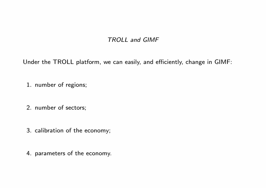
TROLL and GIMF

Under the TROLL platform, we can easily, and e�ciently, change in GIMF:

1. number of regions;

2. number of sectors;

3. calibration of the economy;

4. parameters of the economy.

Structure of a Model Run

All contained in driver.inp:

1. Create the model, and an initial, functional, steady state.

2. Calibrate the model.

3. Simulate the model, using user-speci�ed shocks.

Create the Model

� Model code = a TROLL macro, gimf1.src

{ Written so that you can specify which sectors you want included in (orexcluded from) the resulting model.

{ Flexible number of regions, with names of the user's choosing.

{ each dynamic model equation is paired with an equivalent representationfor the steady-state model.

� Once model code is generated, for speci�c sectors and regions, we simulatean initial "vanilla" steady state, with a symmetric (and simpli�ed) calibrationof all the exogenous variables and parameters.

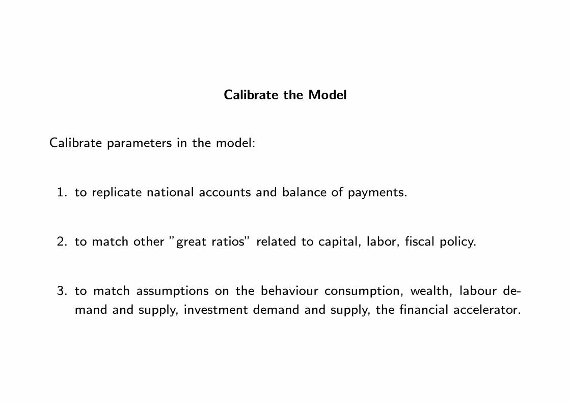
Calibrate the Model

Calibrate parameters in the model:

1. to replicate national accounts and balance of payments.

2. to match other "great ratios" related to capital, labor, �scal policy.

3. to match assumptions on the behaviour consumption, wealth, labour de-

mand and supply, investment demand and supply, the �nancial accelerator.

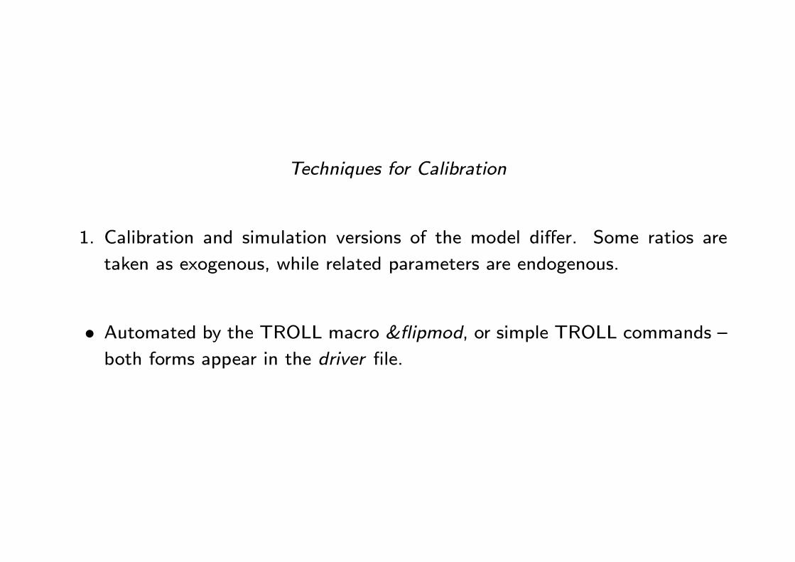
Techniques for Calibration

1. Calibration and simulation versions of the model di�er. Some ratios are

taken as exogenous, while related parameters are endogenous.

� Automated by the TROLL macro & ipmod, or simple TROLL commands {both forms appear in the driver �le.

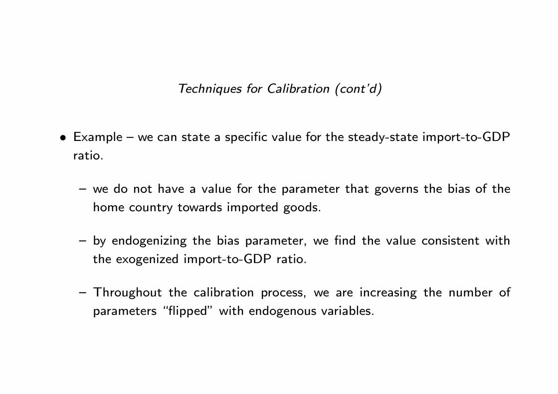
Techniques for Calibration (cont'd)

� Example { we can state a speci�c value for the steady-state import-to-GDPratio.

{ we do not have a value for the parameter that governs the bias of the

home country towards imported goods.

{ by endogenizing the bias parameter, we �nd the value consistent with

the exogenized import-to-GDP ratio.

{ Throughout the calibration process, we are increasing the number of

parameters \ ipped" with endogenous variables.

More Techniques for Calibration

2. It is hard to simulate the model with a new value for the parameter. We

need to gradually move the parameter from its old value to a new value.

� Example { The intertemporal elasticity of substitution of consumption is 0.2;we want a value of 0.5. The model will not simulate at the new value.

{ But, it will simulate at 0.25 easily.

More Techniques for Calibration (cont'd)

� Calibrating the intertemporal elasticity of substitution of consumption.

{ Solution? - Simulate the model at 0.25, save the answer; simulate again

at 0.30; save the answer; simulate repeatedly at 0.05 increments until

the intertemporal elasticity of substitution of consumption is at 0.5.

� This process is called the DAC (divide-and-conquer) algorithm. This processis automated by the TROLL macro &dac, which is used throughout the

driver �le.

Simulate the Model

Based on code found in the TROLL macro &runshocks.

1. Specify the shock in the �le that generates &runshocks.

{ Not just restricted to single impulse responses. Can do a combination

of shocks, both temporary and permanent.

2. Some minimal format requirements in &runshocks ensure that the shock

can be simulated using one of the methods contained in the TROLL macro

&simshock.

Simulation Methods

� Three di�erent simulation routines contained in the TROLL macro&simshocks.

� User should be aware of them, but the macro does not require any userintervention.

Non-linear Simulation

� Based on the native TROLL simulation methods using a Newton-Raphsonalgorithm, and stacked time.

� Can be improved using the DAC (divide-and-conquer) algorithm - run the

shock in increments.

{ after each increment, save the simulation results, and use then as the

starting point for the next increment.

Linear Simulation

Two methods:

1. Numeric linearization around a local steady state - good for temporary and

permanent shocks.

{ The non-linear model is simulated. However, the shocks to be simulated

are divided by a numeric factor to linearize the model.

{ The model solution (relative to the steady-state) is then multiplied up

by the same factor, and shown stacked on the steady-state solution.

Linear Simulation (cont'd)

2. First-order Taylor expansion of the model around a steady-state - good for

temporary shocks.

{ Same linearization technique as in DYNARE. Has been tested with the

GEM, not yet with GIMF.

Simulation Output

Postscript �les, generated by FAME:

� reportss.ps { Reports of the steady-state model simulation.

� Graphs of all the output of the dynamic model simulation.

{ all together { fullpack.ps, for each country.

{ sets of numbered graphs (18 per country).

The DYNARE Platform

Free add-in for MatLab { many canned routines and capabilities. It is especiallygood for:

1. estimation (maximum likelihood, Bayesian).

2. stochastic simulation and impulse responses.

3. monetary policy work - determine optimal simple rules; optimal rules; Taylorfrontiers.

4. welfare analysis.

More on the DYNARE Platform

1. Easy to use { comprehensive instruction manual.

2. Can integrate easily with MatLab capabilities { such as making good graph-

ics of simulation results.

3. Can use non-linear models.

4. Provides checking of model stability { ensures that Blanchard-Kahn condi-

tions hold.

DYNARE and Model Simulation

� DYNARE can linearize or log-linearize nonlinear models around a steady-state.

{ either as a �rst-order or second-order Taylor approximation.

� can use a prespeci�ed numeric steady-state, or it can use the nonlinearmodel to determine the numeric steady state.

� there is also code, compatible with DYNARE, in development, that allowsfor the easy coding of symmetric multi-region models.

A Typical DYNARE File

DYNARE �les are self-contained, with sections describing, in order:

1. the list of endogenous variables (VAR).

2. the lists of exogenous variables (VAREXO), and parameters (PARAME-

TERS).

{ followed by their values { sometimes this section is placed after the model

code.

A Typical DYNARE File (cont'd)

3. MODEL: model code.

{ can be written in fully nonlinear form, including implicit functions.

4. INITVAL: initial values for the model { can be a complete steady state, or

just starting values.

Model-Use Commands

Commands that use / simulate the model include (roughly in order of execution):

1. STEADY : computes the numeric steady state.

2. CHECK : linearizes the model around the steady state, and checks the Blan-

chard Kahn conditions for stability.

Model-Use Commands (cont'd)

3. Any other task you wish to do - estimation, stochastic simulation (for im-

pulse responses), optimal rules, taylor frontiers, etc.

{ Usually consists of set-up (i.e.standard errors of shocks; distributions

of parameters to be estimated; priors), followed by the main command

(ESTIMATE, STOC SIMUL, OSR).

Using Advanced Modelling Files in DYNARE

DYNARE can be used to code up complex models { i.e. multi-region, not fully

calibrated, as in the driver �le for TROLL.

� Uses the work of S�ebastien Villemot of the Banque de France.

� An example is GIMF.

GIMF as an Advanced DYNARE �le

1. Model code can be written, exploiting the MatLab programming language,

in terms of equations for a single region.

{ Using looping structures, similar to those in TROLL, the code can be

replicated for as many regions as desired.

2. Parameters can be recalibrated using the DAC algorithm during the STEADY

command, with the HOMOTOPY option.

Further Reading, Listening and Learning

There are a number of resources for TROLL and DYNARE available online:

1. douglaslaxton.org - especially the TROLL online training, which explains

Newton methods, and how they are exploited for the divide and conquer

(DAC) strategy and algorithm.

2. www.dynare.org { download (portal to downloading versions of DYNARE);

documentation (includes the excellent user's guide; the DYNARE manual).

� more material will follow as a result of this workshop, over the next month.