tropical cyclone wind retrievals from the advanced

Tropical Cyclone Wind Retrievals from the Advanced Microwave Sounding Unit:Application to Surface Wind Analysis

KOTARO BESSHO

Japan Meteorological Agency/Meteorological Research Institute, Tsukuba City, Ibaraki, Japan

MARK DEMARIA

Office of Research and Applications, NOAA/NESDIS, Fort Collins, Colorado

JOHN A. KNAFF

Cooperative Institute for Research in the Atmosphere, Colorado State University, Fort Collins, Colorado

(Manuscript received 27 December 2004, in final form 4 August 2005)

ABSTRACT

Horizontal winds at 850 hPa from tropical cyclones retrieved using the nonlinear balance equation, wherethe mass field was determined from Advanced Microwave Sounding Unit (AMSU) temperature soundings,are compared with the surface wind fields derived from NASA’s Quick Scatterometer (QuikSCAT) andHurricane Research Division H*Wind analyses. It was found that the AMSU-derived wind speeds at 850hPa have linear relations with the surface wind speeds from QuikSCAT or H*Wind. There are alsocharacteristic biases of wind direction between AMSU and QuikSCAT or H*Wind. Using this informationto adjust the speed and correct for the directional bias, a new algorithm was developed for estimation of thetropical cyclone surface wind field from the AMSU-derived 850-hPa winds. The algorithm was evaluated intwo independent cases from Hurricanes Floyd (1999) and Michelle (2001), which were observed simulta-neously by AMSU, QuikSCAT, and H*Wind. In this evaluation the AMSU adjustment algorithm for windspeed worked well. Results also showed that the bias correction algorithm for wind direction has room forimprovement.

1. Introduction

Tropical cyclone (TC) wind observations are ob-tained in a variety of ways. In situ surface observationsinclude those from surface stations, buoys, and ships,and upper-air observations include those from radio-sondes, aircraft reconnaissance, and global positioningsystem (GPS) dropsondes. Winds can also be measuredusing remote sensing such as Doppler radar, microwavescatterometers, and microwave radiometers. Micro-wave scatterometers provide the well-known sea sur-face wind observations from the SeaWinds scatterom-eter on the National Aeronautics and Space Adminis-tration (NASA) Quick Scatterometer (QuikSCAT)

satellite. Microwave radiometers on satellites, such asthe Special Sensor Microwave Imager (SSM/I) on De-fense Meteorological Satellite Program (DMSP), theTropical Rainfall Measuring Mission (TRMM) Micro-wave Imager (TMI), and the Advanced MicrowaveScanning Radiometer Earth Observing System (EOS)(AMSR-E) on Aqua, can only observe wind speed overthe ocean. Wind speed and direction above the surfacecan be retrieved from sequential images from geosta-tionary satellites using feature-tracking methods. Thetraditional method for estimating the TC maximumwind is the Dvorak technique (Dvorak 1975, 1984).

Satellite microwave soundings are also used for esti-mation of TC winds. The first studies of TC surfacewind speed estimation using microwave soundings areby Kidder et al. (1978, 1980). They describe a statisticalmethod to estimate surface wind speed from the 55.45-GHz channel of the Scanning Microwave Spectrometeron Nimbus-6. In these papers, outer surface wind

Corresponding author address: Kotaro Bessho, Japan Meteoro-logical Agency/Meteorological Research Institute, Tsukuba City,Ibaraki 305-0052, Japan.E-mail: [email protected]

MARCH 2006 B E S S H O E T A L . 399

© 2006 American Meteorological Society

JAM2352

speeds were calculated by assuming gradient balanceand using a regression between central pressure and the55.45-GHz temperature anomaly, from which the tem-perature and size of the hurricane warm core can beestimated. Their works were followed by articles fromVelden and Smith (1983), Velden (1989), and Velden etal. (1991) who expanded the use of high-resolution datafrom the Microwave Sounding Unit (MSU) on NationalOceanic and Atmospheric Administration (NOAA)polar-orbiting satellites. Merrill (1995) provided a newalgorithm to more accurately estimate the TC upper-tropospheric warm anomaly from 55-GHz microwaveobservations.

Recently, new microwave sounding systems were in-cluded on NOAA-15, -16, and -17. The Advanced Mi-crowave Sounding Unit (AMSU) is a successor of theMSU, and its applicability to TC analysis was shown byKidder et al. (2000) and Knaff et al. (2000). The besthorizontal resolution of AMSU is 48 km, which is 2times that of MSU. AMSU has also a finer verticalresolution with 15 channels for atmospheric tempera-ture sounding. Using this new instrument, there are sev-eral techniques to estimate wind speed in TCs. A recentextended version of the work of Kidder et al. (1978) isdescribed by Brueske and Velden (2003). They calcu-lated minimum sea level pressure from the brightnesstemperature of the AMSU 54.96-GHz channel with themaximum likelihood regression algorithm developedby Merrill (1995).

Demuth et al. (2004, hereinafter D04) chose an al-ternate approach to the problem of TC intensity esti-mation from AMSU. They calculated 15 physical esti-mators from atmospheric temperature, geopotentialheight, surface pressure, and the gradient wind aroundTCs retrieved from AMSU brightness temperatures.These estimators are the input to a multiple regressionanalysis for TC intensity and wind structure. The Na-tional Hurricane Center (NHC) best track was usedfor the ground truth values of intensity (maximum1-min-sustained surface winds and minimum sea levelpressure), and the wind structure was measured bythe radii of 34-, 50-, and 64-kt winds in four quadrantsrelative to the TC center (1 kt � 0.5144 m s�1). Spencerand Braswell (2001) used a somewhat similar statisticalapproach to estimate the TC maximum wind from sev-eral AMSU channels.

In the studies described above, single TC parameters,such as maximum surface wind speed, central pressure,or wind radii, were estimated. In some cases, subsets ofthe wind field are estimated such as the gradient windas a function of radius in D04, but none of the AMSUTC retrieval methods described above recovers the en-tire wind field. In this paper a new method to estimate

the two-dimensional TC surface wind field is described.The method uses the nonlinear balance equation(Charney 1955) to estimate the three-dimensional windfields from the AMSU-retrieved mass field. The non-linear balance winds at the lowest reliable level (850hPa) are then used to estimate the surface wind. Insection 2 the three-dimensional wind retrieval is brieflydescribed. The datasets used in this study are describedin section 3. In section 4 the wind fields at 850 hPa arecompared with surface wind fields from QuikSCATand H*Wind analyses from the NOAA Hurricane Re-search Division (HRD) of the Atlantic Oceanographyand Meteorology Laboratory (AOML) (Powell et al.1998). Based upon this comparison, an algorithm toconvert the 850-hPa AMSU winds to surface winds isdeveloped. In section 5 this simple algorithm is vali-dated in two cases that were simultaneously observedby AMSU, QuikSCAT, and H*Wind. The results arediscussed and summarized in sections 6 and 7.

The algorithm described in this paper can be used toestimate the horizontal distribution of sea surface windin and around TCs from AMSU brightness temperaturedata. The estimated wind fields have potential applica-tion to the improvement of TC warnings and the ini-tialization of numerical TC prediction models.

2. Three-dimensional AMSU wind retrieval

The AMSU wind retrieval is a generalization of thegradient wind retrieval described by D04. The tempera-ture on an evenly spaced latitude–longitude grid from50 to 920 hPa is determined in the same way as in D04.A statistical retrieval is applied to the AMSU-A radi-ances to determine the temperature profile and the ver-tically integrated cloud liquid water (CLW), which arethen interpolated from the instrument “footprint” lo-cations to a 0.2° latitude � 0.2° longitude grid centeredon the storm. Empirical corrections are applied to thetemperature retrievals to help to account for artificialcooling resulting from attenuation by liquid water andscattering by ice (D04; Linstid 2000). Cases are re-stricted to those in which the storm center was within700 km of the center of the AMSU swath, ensuring thatthere is adequate data coverage over the 12° � 12°analysis domain. Using a National Centers for Environ-mental Prediction (NCEP) global analysis as a lowerboundary condition for surface pressure at the domainboundaries, the hydrostatic equation is integrated up-ward to 50 hPa using the AMSU temperatures to givethe geopotential height as a function of pressure at thelateral boundaries. Virtual temperature effects are ne-glected in all of the hydrostatic integrations. Under theassumption that 50 hPa is above the storm circulation,

400 J O U R N A L O F A P P L I E D M E T E O R O L O G Y A N D C L I M A T O L O G Y VOLUME 45

a smoothness condition is applied to give the geopoten-tial height over the entire domain at 50 hPa. The hy-drostatic equation is then integrated downward to givethe three-dimensional height field. In D04 this heightfield is azimuthally averaged relative to the storm cen-ter and the gradient wind equation is used to determinethe wind at each pressure level as a function of radius.

For the three-dimensional winds the gradient windequation is replaced by the nonlinear balance equation(Charney 1955). On a midlatitude beta plane this equa-tion can be written as

uxux � 2�xuy � �y�y � �� f � �y� � �u � �2� � 0,

�1�

where u and � are the nondivergent horizontal windcomponents, f and are the Coriolis parameter and itsnorthward gradient, respectively, evaluated at the do-main center, is the geopotential, �2 is the horizontalLaplacian operator, and subscripts x and y representeastward and northward derivatives. The properties ofthe nonlinear balance equation are discussed in detailby Paegle and Paegle (1976) and Kasahara (1982). Animportant property of (1) is that it is an elliptic equationprovided that

f 2 � 2�2� � 2�u � 0. �2�

A number of iterative methods have been developed tosolve (1) for the nondivergent wind field given the geo-potential field (e.g., Kasahara 1982; Iversen and Nor-deng 1982). However, it was found that these conven-tional solution methods did not converge for some ofthe stronger TC cases, primarily because of violationsof (2) over small regions near the storm center. For thisreason, a least squares method was used to solve (1).

For the least squares solution, (1) is first written infinite-difference form. Then, the residual of the finite-difference form of (1) at each grid point is defined asRij. The mean square residual is defined as

L � �i�2

I�1

�j�2

J�1

Rij2. �3�

The summation is over all of the points in the analysisdomain except the lateral boundaries. At the bound-aries, u and � are determined from the NCEP analyses.At all interior points, u and � are determined by mini-mizing (3). The minimization is performed using a gra-dient-descent method, where the gradient of L withrespect to u and � at each analysis point is calculated bytaking the derivative of (3) after substitution of thefinite-difference form of (1). The gradient-descent al-gorithm converges much more slowly than the more

standard iterative solutions but is much more robust,especially for the stronger TCs. The method provides uand � at each pressure level from 50 hPa to the surface.

Because the AMSU radiances are attenuated in areaswith large amounts of liquid water, the temperatureretrievals are less reliable in the low levels near thestorm center. A method to partially correct for thisproblem is included in the temperature retrieval algo-rithm as described by D04. However, the wind retriev-als are still considered less reliable below 850 hPa, sothe AMSU winds at 850 hPa will be used in the remain-der of the paper.

3. Data

a. AMSU

This study utilizes the AMSU brightness temperaturedata from NOAA-15 and -16, which are archived in aCooperative Institute for Research in the Atmosphere(CIRA) database for TCs from 1999 to 2002. The caseswere restricted to those of hurricane strength (maxi-mum surface winds of at least 33 m s�1). The data col-lection process is the same as that described in D04, inwhich the AMSU observations around all TCs beingforecast by NHC were saved at 6-h intervals. If newdata were available at a 6-h period and the storm centerwas within 700 km of center of the AMSU swath, thecase was saved in the archive. This procedure resultedin about one case per storm per satellite per day.

b. QuikSCAT

QuikSCAT sea surface wind data archived on a filetransfer protocol (FTP) site of Remote Sensing Systems(RSS) were collected for comparison with the AMSUwind data. The SeaWinds instrument on QuikSCATlaunched in June 1999 is a Ku-band (i.e., a frequencynear 14 GHz) radar. It works as a scatterometer totransmit a radar pulse down to the sea surface and mea-sures the power that is scattered back. The power of thebackscattered radiation is proportional to the oceansurface roughness, which is correlated with the near-surface wind speed and direction. QuikSCAT can easilydetect a TC as a closed circulation in the surface windson the ocean (Katsaros et al. 2001).

In the RSS database, sea surface wind was retrievedfrom QuikSCAT with a geophysical model functioncalled Ku-2001 (Wentz et al. 2001). The wind speed anddirection at a height of 10 m are retrieved from mea-surements of the power of the backscattered radiation.The wind QuikSCAT data correspond to surface windswith a time averaging period of 8–10 min.


c. H*Wind

As will be shown in detail later, both the AMSU andQuikSCAT winds have limitations. To provide “groundtruth,” H*Wind surface wind field analyses were ob-tained from the HRD ftp site. H*Wind was developedto integrate many kinds of wind data such as in situsurface observations, aircraft reconnaissance, GPSdropsonde, and remote sensing observations, into aconsistent surface wind field (Powell et al. 1998). Alldata are quality controlled and processed to conform toa common framework for height (10 m), exposure (ma-rine or open terrain over land), and averaging period(maximum 1-min-sustained wind speed) using resultsfrom micrometeorology and wind engineering (Powellet al. 1996; Powell and Houston 1996). H*Wind analy-ses are provided on an FTP server for research pur-poses, and to NHC hurricane specialists for forecastapplications on a regular 3- or 6-h schedule consistentwith NHC’s warning and forecast cycle. The spatialresolution of H*Wind analyses used in this study varybetween 2.8 and 8.4 km.

The surface wind data synthesized into H*Wind in-clude data from ships, buoys, coastal platforms, andsurface aviation reports. Aircraft reconnaissance dataare adjusted to the surface with a planetary boundarylayer model (Powell 1980). Remote sensing observa-tions in H*Wind can include surface wind speed esti-mates from microwave imagers such as SSM/I and TMIon polar-orbiting satellites, surface wind estimates fromscatterometers on European Remote Sensing Satellite(ERS) and QuikSCAT, low-level cloud drift windsfrom Geostationary Operational Environmental Satel-lites (GOES), and, if available, step-frequency micro-wave radiometer measurements of surface winds fromNOAA WP-3D aircraft. In this paper the H*Windanalyses are used for a comparison with AMSU andQuikSCAT wind estimates. To maintain independenceamong the three types of wind estimates, the H*Windanalyses that did not include QuikSCAT observationswere used in this study.

d. AMSU–QuikSCAT comparison cases

Fifty-seven cases were chosen for comparison of theAMSU and QuikSCAT wind fields. The time differ-ences for the matching cases were less than 1.5 h. Thecases in which there were landmasses such as continentsor large islands in the analysis region were excluded.Footprints in which the QuikSCAT rain flags weremarked for strong rain attenuation were also excludedfrom comparison. Using a Barnes analysis (Barnes1964), the QuikSCAT winds were interpolated to the12° latitude � 12° longitude AMSU analysis grid. The

comparison was then restricted to only those grid pointswithin 500 km of the TC center.

e. AMSU–H*Wind comparison cases

For comparison of the AMSU 850-hPa wind fieldwith the H*Wind surface wind field, 16 cases werefound in which the time difference was less than 3 h.Similar to the comparisons between AMSU andQuikSCAT, cases in which continents or large islandswere located in analysis region were excluded. H*Windhas large (8° latitude � 8° longitude) or small (4° lati-tude � 4° longitude) analysis domains. In this study theH*Wind data in the larger analysis domain were used.Similar to the QuikSCAT data, the H*Wind analyseswere interpolated to the AMSU retrieval grid pointsusing a Barnes analysis, and the comparisons were re-stricted to grid points within 500 km of the storm cen-ter. H*Wind speeds were converted from 1- to 10-minaverages by dividing by 1.1 (Powell et al. 1996).

f. AMSU–QuikSCAT–H*Wind comparison cases

Out of the 57 AMSU cases with matching QuikSCATdata and the 16 cases with matching H*Wind data,there are two cases for which all three wind fields areavailable. These cases were set aside for independentvalidation of the algorithm to convert the AMSU 850-hPa winds to surface values. Thus, all of the analysisdescribed in the next section includes 55 QuikSCATcases and 14 H*Wind cases.

Table 1 shows statistics of wind parameters and cen-tral pressure in the comparison cases. Statistics of maxi-mum wind and central pressure can be calculated fromall comparison cases, but wind radii of 34, 50, and 64 ktfor four directions (northeast, southeast, southwest,northwest) can be averaged only from the cases inwhich those wind speed thresholds are archived. Fromthe upper table, the maximum wind speeds in each setof comparison cases have about the same average value( 30 m s�1). However, from the lower table, theAMSU–H*Wind comparison cases have 1.5–2 timesthe wind radii of AMSU–QuikSCAT comparison cases.

Figure 1 shows the locations of TCs in the comparisoncases. This figure shows that TCs in AMSU–QuikSCATcomparison cases were distributed over all western At-lantic Ocean and eastern Pacific Ocean basins exceptfor the Caribbean Sea and Gulf of Mexico. On theother hand, TCs in the AMSU–H*Wind comparisoncases are restricted to the far western side of the At-lantic basin because they all include aircraft reconnais-sance data. According to Table 1, the average centralpressure for the AMSU–H*Wind cases is 983 hPa ascompared with 992 hPa for the AMSU–QuikSCAT


cases. The storms in H*Wind cases tend to be moremature than in QuikSCAT cases. The uneven spatialdistribution of the TCs in H*Wind cases probably ex-plains the wind radii difference between the AMSU–H*Wind and AMSU–QuikSCAT comparison casesmentioned above.

4. Comparison of AMSU 850-hPa winds withQuikSCAT and H*Wind

Figure 2 shows scatterplots of wind speed and direc-tion from the 850-hPa AMSU winds and the Quik-SCAT surface wind field (Fig. 2a) and the H*Windsurface wind field (Fig. 2b) for the matching cases. TheQuikSCAT comparison includes 84 576 grid pointsfrom the 55 cases, and the H*Wind comparison includes

22 217 grid points from the 14 matching cases. Statisticsof the comparisons are summarized in Table 2.

Figure 2a shows that the QuikSCAT surface windspeed reached almost 60 m s�1 but the AMSU windspeed only reaches about 40 m s�1. The new RSS Quik-SCAT retrieval is supposed to measure surface windsabove 30 m s�1 (Wentz et al. 2001). Figure 2a showsthat some estimates are considerably higher than 30m s�1. The maximum wind speed differences are be-cause of many factors, such as the very different way inwhich the winds are estimated, geophysical noise result-ing from rain attenuation and ice scattering, and thetemporal variability of wind speed. However, the big-gest reason for the difference is considered to be thehorizontal resolution difference between AMSU andQuikSCAT. According to Quilfen et al. (1998), the

FIG. 1. Locations of TCs in the comparison cases. Filled circles are locations in the comparison cases forAMSU and QuikSCAT and open squares are those for AMSU and H*Wind.

TABLE 1. Statistics of the TC wind parameters and central pressures in the comparison cases. The upper table shows the maximumwind speed and central pressure statistics, and the lower table shows the average radii of 34-, 50-, and 64-kt winds for the four quadrants(northeast, southeast, southwest, northwest) relative to the storm center.

Avg Max Min Std dev

AMSU–QuikSCAT (55 cases)Max wind speed (m s�1) 28 72 13 14Central pressure (hPa) 992 1010 921 19

AMSU–H*Wind (14 cases)Max wind speed (m s�1) 35 59 10 15Central pressure (hPa) 983 1013 924 25

Northeast Southeast Southwest Northwest

AMSU–QuikSCAT (45 cases)34-kt wind radii (km) 173 151 125 14650-kt wind radii (km) 75 56 51 6364-kt wind radii (km) 24 22 17 22

AMSU–H*Wind (13 cases)34-kt wind radii (km) 269 221 177 20950-kt wind radii (km) 158 100 89 10864-kt wind radii (km) 63 37 33 50


fine-horizontal-resolution data of the scatterometerdata (ERS in their case) enable the detection of fairlyhigher wind speeds in TCs. The finest AMSU horizon-tal resolution is 48 km, while QuikSCAT has a resolu-tion of 25 km. Thus, QuikSCAT can better resolve theinner-core region of TCs, which is consistent with Fig.2a in the high-wind regime. Except for the grid points inwhich the QuikSCAT wind speed is much higher thanAMSU, most of the points are spread evenly aroundthe dotted line in Fig. 2a where the AMSU wind speedis equal to the QuikSCAT wind speed. As shown in

TABLE 2. Statistics of the comparisons of AMSU wind speedand direction at 850 hPa with QuikSCAT or H*Wind; MAD:mean absolute difference; COR: correlation coefficient betweenAMSU and QuikSCAT, or H*Wind.

Bias MAD COR

QuikSCATWind speed (m s�1) �1.49 4.10 0.609Wind direction (°) 14.8 42.7 0.519

H*WindWind speed (m s�1) �0.59 4.91 0.533Wind direction (°) 13.4 38.1 0.621

FIG. 2. Scatter diagrams of (a) AMSU wind at 850 hPa vs QuikSCAT surface wind, and (b) AMSU wind at 850hPa vs H*Wind surface wind. The diagrams on the left side are for wind speed, and the diagrams on the right sideare for wind direction.


Table 2, the AMSU wind speed bias relative to Quik-SCAT is �1.5 m s�1, and the mean absolute difference(MAD) is almost 4 m s�1. The correlation coefficientbetween the AMSU and QuikSCAT wind speeds is0.609.

Similar results are found in the comparison of AMSUwinds with H*Wind surface winds as shown in Fig. 2b.The maximum wind speed of H*Wind is almost 60m s�1, but the maximum AMSU wind speed is onlyabout 40 m s�1. This speed difference is also related todiffering horizontal resolution. As mentioned previ-ously, the resolution of the H*Wind analyses rangedfrom 2.8 to 8.3 km in the 14 comparison cases, whichwas necessary to resolve the aircraft data. The bias ofthe AMSU wind speed relative to H*Wind is �0.6m s�1 in Table 2. The MAD of the wind speed is about5 m s�1, which is larger than the MAD between AMSUand QuikSCAT, and the correlation coefficient ofAMSU and H*Wind wind speed is 0.533, which issmaller than that of AMSU versus QuikSCAT.

The statistics of wind direction differences are com-plicated by the fact that 0° and 360° have the samemeaning. Recently, “circular statistics” were developed(Fisher 1993; Jammalamadaka and SenGupta 2001) tohandle this problem. Statistical parameters such as themean absolute difference, standard deviation, bias, andcorrelation coefficient for wind direction in this paperwere calculated by circular statistics.

As shown in Fig. 2a and Table 2, the MAD of winddirection between AMSU and QuikSCAT is about 40°and the bias is 14.8°. The directional bias was defined asAMSU minus QuikSCAT, which indicates that theAMSU wind direction is larger than the mean Quik-SCAT wind direction. Assuming cyclonic flow, theQuikSCAT surface wind direction turns inward towardthe hurricane center by about 15° from the direction ofthe AMSU wind at 850 hPa. This result is consistentwith previous studies of TC wind structure. For ex-ample, Frank (1977) found mean inflow angles within200–700 km of northwest Pacific TCs to be 23°–25° atthe surface and 3°–8° at 850 hPa. Thus, the surfacewinds turned inward about 19° relative to the 850-hPawinds, which is similar to the bias of AMSU wind di-rection relative to the QuikSCAT wind direction.

Similar results are found in the comparison of AMSUand H*Wind wind directions, as shown in Table 2. TheMAD is about 40° and the bias is consistent with theexpected inflow angles at 850 hPa and the surface. Thelarge mean absolute differences and biases can be seenin the scatterplots of wind directions in Fig. 2b. Thecorrelation coefficient between AMSU and H*Windwind directions is better than that for the comparison ofAMSU with QuikSCAT. This improved correlation is

probably because of the fact that the QuikSCAT winddirections also sometimes have substantial errors.

As briefly described in section 2, empirical adjust-ments are applied to help to correct the AMSU tem-perature soundings for attenuation by liquid water andscattering by ice. Although these corrections improvethe retrievals as described by D04, there are still errorsresulting from these effects, especially in regions ofdeep convection near the storm centers. To further in-vestigate this issue, the AMSU wind retrievals will bestratified as a function of convective activity. For thispurpose, the AMSU-retrieved CLW will be used as aproxy for convection.

Before stratifying the AMSU wind comparisons, theAMSU-retrieved CLW is compared with GOES infra-red brightness temperatures (TB) to provide somephysical insight into the accuracy of the CLW values.For this purpose the GOES channel-4 (10.7 �m) TB forthe 55 AMSU–QuikSCAT comparison cases were ob-tained from an archive at CIRA. Because the GOESdata are available at time intervals that are usually nolonger than 0.5 h, the GOES data are very close in timeto the AMSU data. The AMSU CLW values andGOES TB were azimuthally averaged at 20-km radialintervals from the TC centers. This procedure resultedin 984 points with TB colder than 273 K. If TB werewarmer than 273 K, the point was regarded as a near-surface sea or land temperature and was not included inthe comparison.

Figure 3 shows a scatterplot of the azimuthally aver-aged TB versus CLW, where an exponential regressioncurve is shown by a solid line. The determination coef-ficient of this curve is 0.426. As shown by Negri andAdler (1993), a TB value of 235 K is often used as a

FIG. 3. Scatter diagram of tangentially averaged TB vs azimuth-ally averaged CLW. The solid line shows exponential regressioncurve and the formula in the diagram shows its equation.


threshold for the identification of convective areas.From the regression curve in Fig. 3, a CLW value of0.44 mm corresponds to a TB value of 235 K. Thus,CLW � 0.44 mm will be used as a threshold for sepa-rating convective and nonconvective points in theAMSU analysis domain. Generally, CLW in convectiveclouds is larger than that in stratiform clouds and CLWhas larger values in more developed convective clouds.If CLW � 1.32 mm, the region is regarded as being“highly” convective. From the regression curve in Fig.3, a CLW value of 1.32 mm corresponds to a TB valueof 200 K.

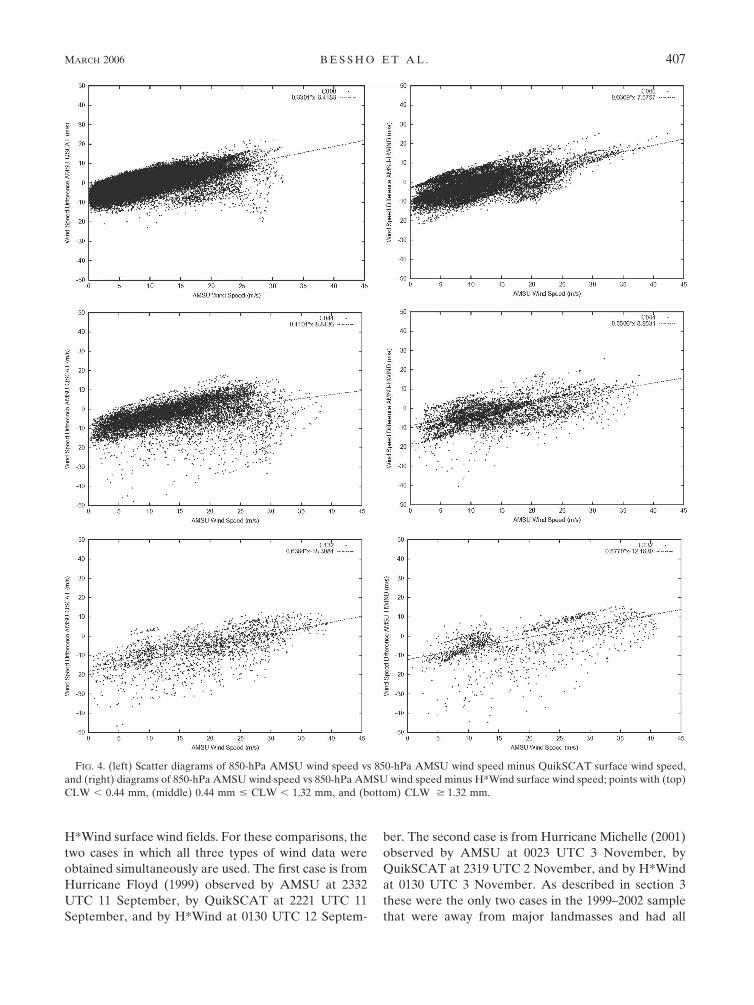
Figure 4 (left column) shows scatter diagrams of theAMSU–QuikSCAT wind differences versus AMSUwind speeds, stratified into nonconvective, convective,and highly convective regions. In each scatterplot leastsquares linear regressions are shown by dotted lines.Rain-flagged QuikSCAT data were detected by micro-wave brightness temperature observations from SSM/Iand TMI (Wentz et al. 2001). On the other hand, con-vective and highly convective region were estimatedfrom the value of AMSU CLW. As already mentionedabove, QuikSCAT data with strong rain flags were ex-cluded in this analysis, but there are still convective andhighly convective regions because of the difference ofthese two estimation methods. The correlation coeffi-cients, the slopes, and intercepts of the regression linesfor each scatterplot in Fig. 4 are shown in Table 3. Forall three stratifications on the left side of Fig. 4 there isa positive correlation between the AMSU winds andthe AMSU–QuikSCAT difference. The y intercept forthe highly convective region is the largest (�18 m s�1),which indicates the largest bias of the AMSU windspeeds relative to the QuikSCAT speeds for the lowAMSU wind speed cases. The y intercepts for the non-convective and convective regions are also negative butare considerably smaller in magnitude than for thehighly convective cases. The threshold values of AMSUwind speed between negative and positive AMSU–QuikSCAT differences also increases with each CLWstratification. For high values of AMSU wind speed inFig. 4 the AMSU values are on average higher than theQuikSCAT winds, which is expected because Quik-SCAT measures at the surface but AMSU is at 850 hPa.

Results similar to those described above are found incomparisons between AMSU wind speed at 850 hPaand the AMSU–H*Wind differences as shown in theFig. 4 (right column) and Table 3. In the comparisonswith H*Wind the correlation coefficients in all CLWcategories are above 0.60. The linear regressions havealmost the same slopes ( 0.60), and intercepts rangefrom �7.6 to �12.2 m s�1. In the highly convective ar-

eas, the intercept in the AMSU–H*Wind difference isless than that for the AMSU–QuikSCAT difference.

Figure 5 shows the dependency of the wind directiondifference between AMSU wind and QuikSCAT onAMSU wind speed. The mean and standard deviationof the wind direction differences in 5 m s�1 AMSUwind speed intervals are also shown in Fig. 5. For lowAMSU wind speeds (�10 m s�1), the wind directiondifferences vary widely from �180° to �180°. ForAMSU wind speeds greater than 10 m s�1, the standarddeviations of wind directional differences decrease andconverge to near zero. The averaged differences ofwind direction range from 12° to 25°. As described pre-viously, a positive difference means that the AMSUwind at 850 hPa turns less inward toward the TC centerthan does the QuikSCAT surface wind. To adjust theAMSU wind direction at 850 hPa to the surface wind,the direction must be turned inward slightly.

The same trend is found for the dependence of theAMSU–H*Wind direction difference on the AMSUwind speed, except for a small negative bias at the low-est AMSU wind speeds in Fig. 5 and Table 3.

From these comparisons described above, theAMSU winds have some systematic differences fromthe QuikSCAT and H*Wind winds. The wind speeddifferences between the AMSU wind at 850 hPa andthe surface winds are proportional to the AMSU windspeed itself. The wind direction differences of AMSUand the two surface wind datasets also have biases thatdepend on the AMSU wind speed. Using these rela-tionships, the TC surface wind distribution retrievedfrom the 850-hPa AMSU winds can be converted tosurface wind. The surface wind speed is retrieved fromthe AMSU wind speed at 850 hPa with a regressionmodel. The surface wind direction is obtained from theAMSU wind direction at 850 hPa minus the bias as afunction of the AMSU wind speed. Two sets of AMSUsurface wind adjustment relationships were derived.The adjustments derived from the AMSU–QuikSCATcomparison are called QCOM (Table 4) and the adjust-ments from H*Wind are called HCOM (Table 5). Inthe relationships shown in Tables 4 and 5, WSsurfmeans surface wind speed, and WSamsu means AMSUwind speed at 850 hPa; WD (°) is the abbreviation forwind direction, and subscripts are the same as for WS(m s�1). Validations of these relationships applied tothe AMSU 850-hPa winds to provide surface winds aredescribed in the next section for two independent cases.

5. Validations of retrieval methods of surface wind

To validate the QCOM and HCOM adjustments,these methods are applied to AMSU wind fields at 850hPa and compared with corresponding QuikSCAT and


H*Wind surface wind fields. For these comparisons, thetwo cases in which all three types of wind data wereobtained simultaneously are used. The first case is fromHurricane Floyd (1999) observed by AMSU at 2332UTC 11 September, by QuikSCAT at 2221 UTC 11September, and by H*Wind at 0130 UTC 12 Septem-

ber. The second case is from Hurricane Michelle (2001)observed by AMSU at 0023 UTC 3 November, byQuikSCAT at 2319 UTC 2 November, and by H*Windat 0130 UTC 3 November. As described in section 3these were the only two cases in the 1999–2002 samplethat were away from major landmasses and had all

FIG. 4. (left) Scatter diagrams of 850-hPa AMSU wind speed vs 850-hPa AMSU wind speed minus QuikSCAT surface wind speed,and (right) diagrams of 850-hPa AMSU wind speed vs 850-hPa AMSU wind speed minus H*Wind surface wind speed; points with (top)CLW � 0.44 mm, (middle) 0.44 mm � CLW � 1.32 mm, and (bottom) CLW � 1.32 mm.


three data types available. These two cases were with-held from the development of the QCOM and HCOMrelationships to provide an independent sample. As athird wind estimate, NCEP global model surface analy-ses are also used to assess the quality of the QCOM and

HCOM adjustments. NCEP analyses for the validationare at 0000 UTC 12 September for Floyd and 0000 UTC3 November for Michelle. The purpose of including theNCEP winds is to determine if the AMSU algorithmhas any advantage over what is possible from the as-similation of operational data sources. The AMSU sur-face wind fields could also have been compared with insitu wind data such as buoys. However, these data arevery sparse, and the H*Wind analyses already includethem when available.

Figure 6 shows the wind fields for Floyd from AMSUat 850 hPa (Fig. 6a), QuikSCAT (Fig. 6b), H*Wind(Fig. 6c), and NCEP (Fig. 6d). The CLW field esti-mated from AMSU is also shown in Fig. 7. The 850-hPaAMSU wind field in Fig. 6a does not include the modi-fication by QCOM or HCOM (hereinafter NOMO).The wind speed distribution of AMSU above 12 m s�1

is similar to the wind speed distribution of QuikSCAT(Fig. 6b). The high-speed region is asymmetric and islocated in the direction from north to southeast of thehurricane center, similar to a rainband. The distribution

FIG. 5. Scatter diagrams of 850-hPa AMSU wind speed vs 850-hPa AMSU wind directions (top left) minus QuikSCAT surface winddirection and (top right) minus H*Wind surface wind direction. (bottom) Histograms of the total grid numbers, the mean wind directiondifferences, and bars of standard deviation of the wind direction differences in 5 m s�1 intervals of 850-hPa AMSU wind speeds:comparison with (bottom left) QuikSCAT and (bottom right) H*Wind.

TABLE 3. Statistics of the comparisons of AMSU wind speed at850 hPa with the wind speed difference between AMSU at 850hPa and QuikSCAT or H*Wind surface winds, stratified by cloudliquid water amount.

No. ofdata Slope Intercept COR

QuikSCATCLW � 0.44 mm 72 166 0.63 �6.42 0.7090.44 mm � CLW

� 1.32 mm10 466 0.41 �8.84 0.439

1.32 mm � CLW 1964 0.64 �18.31 0.624H*Wind

CLW � 0.44 mm 16 265 0.67 �7.58 0.6950.44 mm � CLW

� 1.32 mm4618 0.55 �8.95 0.627

1.32 mm � CLW 1334 0.58 �12.16 0.612


of CLW roughly corresponds to the distributions ofwind speed above 12 m s�1 (Fig. 7). The AMSU windspeed distribution above 18 m s�1 is wider along thedirection from north to south than that of QuikSCATwinds. It can also be seen that the AMSU wind speeddistribution above 18 m s�1 is narrower in the east–westdirection than that of QuikSCAT. The AMSU windspeed field has some patches of weak speed below 2m s�1 located on the west side of the strong wind speedarea already mentioned. The H*Wind wind speed dis-tribution in Fig. 6c is different from those of AMSUor QuikSCAT. The wind speed distribution of H*Windis almost symmetric, and there is no band-type highwind speed area in the distribution. Thus, neither theAMSU nor QuikSCAT retrievals are able to capturethe intense inner core of the storm because of the hori-zontal resolution limitations described previously. TheNCEP surface wind analysis also shows an asymmetric

distribution, which is similar to those of AMSU andQuikSCAT (Fig. 6d).

The AMSU wind direction near the hurricane centerhas a structure similar to that for QuikSCAT, H*Wind,and NCEP, with a general counterclockwise rotation.However, in the outer region of the hurricane centerthe AMSU wind direction distribution shows remark-able differences from those of QuikSCAT, H*Wind,and NCEP, which still show counterclockwise circula-tions away from the storm center. Especially in theweak wind speed regions of AMSU there are somesmall vortices, which are widely different from an idealdistribution of wind direction in TCs. The small vorticesare likely artifacts of the AMSU retrieval techniquebecause of the problems of liquid water attenuation orice scattering.

The wind fields from the four data types for the Hur-ricane Michelle case (not shown) are fairly similar tothe results for Floyd. Generally, the two satellite windfields show similar structures, where the high windspeed region is located on the periphery of the hurri-cane center with speeds lower than in the H*Windanalyses, and the speed gradually decreases away fromthe storm center. Wind directions show counterclock-wise circulation near the storm center. The NCEP sur-face wind field for the Michelle case is different fromother three wind fields. The center of rotation ofMichelle in the NCEP wind field is located on north-eastern side of those of other three wind fields. TheAMSU wind speed distribution shows several weakspeed patches below 6 m s�1 away from the hurricanecenter, with small vortices similar to those in the Floydcase. These features were not seen in the QuikSCAT,H*Wind, or NCEP wind fields.

Figure 8 shows the surface wind field retrieved fromthe AMSU wind at 850 hPa using the QCOM (Fig. 8a)and HCOM (Fig. 8b) adjustments for the Floyd case.When QCOM is compared with the QuikSCAT surfaceimage (Fig. 6b), it is easily seen that the wind speeddistribution of QCOM more closely resembles thatof QuikSCAT than the original AMSU wind field(NOMO). It has also similar characters with the NCEPwind field. In QCOM, the wind speed area above 12m s�1 spreads in the east–west direction, but the strong-est wind region above 24 m s�1 is shortened in thenorth–south direction. The weak wind speed patchesaway from the hurricane center in NOMO have almostdisappeared in QCOM. Similar tendencies are alsofound in HCOM, but the strongest wind region near thecenter has shrunk excessively. The asymmetric windspeed distribution of QCOM and HCOM are still con-siderably different from the very symmetric H*Winddistribution.

TABLE 4. QCOM: surface wind retrieval method derived fromcomparison with QuikSCAT.

WSWSsurf � [(1 � 0.63)

� WSamsu] � 6.42(CLW � 0.44 mm)

WSsurf � [(1 � 0.41)� WSamsu] � 8.84

(0.44 � CLW � 1.32 mm)

WSsurf � [(1 � 0.64)� WSamsu] � 18.31

(1.32 � CLW mm)

WDWDsurf � WDamsu � 12.60 (WSamsu � 5 m s�1)WDsurf � WDamsu � 12.30 (5 � WSamsu � 10 m s�1)WDsurf � WDamsu � 15.02 (10 � WSamsu � 15 m s�1)WDsurf � WDamsu � 18.30 (15 � WSamsu � 20 m s�1)WDsurf � WDamsu � 22.35 (20 � WSamsu � 25 m s�1)WDsurf � WDamsu � 23.81 (25 � WSamsu � 30 m s�1)WDsurf � WDamsu � 25.08 (30 � WSamsu � 35 m s�1)WDsurf � WDamsu � 21.08 (35 � WSamsu)

TABLE 5. HCOM: same as Table 4, but for H*Wind.

WSWSsurf � [(1 � 0.67)

� WSamsu] � 7.58(CLW � 0.44 mm)

WSsurf � [(1 � 0.55)� WSamsu] � 8.95

(0.44 � CLW � 1.32 mm)

WSsurf � [(1 � 0.58)� WSamsu] � 12.16

(1.32 � CLW mm)

WDWDsurf � WDamsu � 2.78 (WSamsu � 5 m s�1)WDsurf � WDamsu � 8.62 (5 � WSamsu � 10 m s�1)WDsurf � WDamsu � 15.34 (10 � WSamsu � 15 m s�1)WDsurf � WDamsu � 16.98 (15 � WSamsu � 20 m s�1)WDsurf � WDamsu � 19.45 (20 � WSamsu � 25 m s�1)WDsurf � WDamsu � 20.92 (25 � WSamsu � 30 m s�1)WDsurf � WDamsu � 17.29 (30 � WSamsu � 35 m s�1)WDsurf � WDamsu � 18.67 (35 � WSamsu � 40 m s�1)WDsurf � WDamsu � 8.28 (40 � WSamsu m s�1)


FIG. 6. (a) The 850-hPa AMSU wind distribution, (b) QuikSCAT surface wind distribution, (c) H*Wind surfacewind distribution, and (d) surface wind distribution of NCEP global model analyses for Hurricane Floyd (1999).The contour interval for wind speed is 2 m s�1. The wind direction is indicated by the white arrows, and the arrowlength is proportional to the wind speed.


Fig 6 live 4/C

Wind direction differences away from the hurricanecenter of QCOM or HCOM become smaller than thatof NOMO as compared with the QuikSCAT, H*Wind,or NCEP surface winds. However, the small vortices,corresponding to weak wind speed regions located onthe west side of the periphery of the center, still exist inQCOM and HCOM.

The QCOM and HCOM surface winds for theMichelle case were also compared with the QuikSCAT,H*Wind, NCEP, or NOMO wind fields (not shown),and the results were similar to the Floyd case. Thestrong wind speed distribution in QCOM is more simi-lar to that of QuikSCAT and H*Wind than NOMO.The NCEP surface wind field for the Michelle case didnot resemble the QCOM field. The weak wind regionson periphery of the center were reduced in QCOM, butthe small vortices seen in NOMO still exist. HCOMshows the same features as QCOM except for the maxi-mum wind speed, which is lower than that of QCOM.

Table 6 shows statistical results for comparisons ofthe three kinds of AMSU wind retrievals (NOMO,QCOM, and HCOM) and the surface winds of Quik-SCAT for the combined sample from Hurricanes Floyd

and Michelle. Statistics of the comparisons of the sur-face wind of NCEP with the surface wind of QuikSCATfor the cases of Hurricanes Floyd and Michelle are alsoshown as reference. This table shows that the QCOMadjustment improves the AMSU wind speed retrievalrelative to the NOMO case. The NOMO correlationcoefficient and MAD are 0.589 and 5.48 m s�1, respec-tively. For QCOM, the correlation coefficient increasesto 0.776 and the MAD is reduced to 3.40 m s�1. Thewind speed improvements for the HCOM adjustmentsare similar to (but not quite as good as) those forQCOM, with a correlation coefficient and MAD of0.753 and 3.58 m s�1, respectively. The NCEP windspeed MAD from QuikSCAT is comparable to thatfrom NOMO and a little larger than those for QCOMand HCOM.

The improvements in the AMSU wind direction forthe QCOM or HCOM adjustments are not as good asthose for wind speed. The MAD for NOMO in Table 6is 34.4°, which reduces only slightly to 33.6° and 33.0°for QCOM and HCOM, respectively. The correlationcoefficients for QCOM and HCOM are a little smallerthan that for NOMO. The NCEP wind directions showsbetter results than do those of QCOM and HCOM,especially for the MAD and the correlation coeffi-cients. The differences between the results of threekinds of AMSU winds (NOMO, QCOM, and HCOM)and NCEP surface winds are probably because of thespurious vortices away from the storm center in theAMSU analyses. These results indicate that the simplealgorithm to modify the AMSU wind direction by sub-tracting the bias as a function of AMSU wind speed hassome limitations.

The results from comparisons between the H*Windsurface wind and three AMSU wind fields (NOMO,QCOM, and HCOM) are shown in Table 7. The statis-tical results from comparisons between the H*Windand NCEP surface winds are also shown. The resultsgenerally are similar to those for the comparison withQuikSCAT in that the QCOM and HCOM proceduresimprove the wind speed error more than the wind di-rection error. However, the correlation coefficients aresmaller and the MADs are larger in the comparisonswith H*Wind than in those with QuikSCAT. This deg-radation in the comparison is primarily because of thefact that the H*Wind analyses resolve the inner core ofthe storm, but the AMSU and QuikSCAT analyses donot. Similar to the comparison with QuikSCAT, NCEPshows comparable results to QCOM and HCOM in theMAD for wind speed, and better results than QCOMand HCOM in the MAD and the correlation coeffi-cients for wind direction. Because of the aircraft data inH*Wind, the comparisons with AMSU and NCEP are

FIG. 7. AMSU cloud liquid water distribution for HurricaneFloyd (1999). The contour interval for CLW is 2 mm.


Fig 7 live 4/C

measures of the accuracies of these two methods. Thisresult indicates that in the vicinity of TCs, the AMSUretrievals have comparable accuracy to global data as-similation systems.

Table 8 shows the results from comparisons betweenthe NCEP surface wind and the three AMSU windfields (NOMO, QCOM, and HCOM). Almost the sameresults are found in this table as previously mentionedin the discussion of Tables 6 and 7. QCOM and HCOMimprove the correlation coefficients for wind speed, butthe values of the coefficients are lower than other twovalidations with QuikSCAT and H*Wind. The winddirection retrieval algorithm in QCOM and HCOMagain do not show much improvement. In these statis-tics, the bias of wind direction in QCOM and HCOMshows the same (but negative) magnitude as that inNOMO.

6. Discussion

One purpose of this paper is a comparison of thewind field retrieved from AMSU temperature data us-

ing the nonlinear balance equation at 850 hPa with sur-face wind fields obtained from QuikSCAT or H*Wind.The second objective is to use the results of the com-

TABLE 6. Statistics of the comparisons of the three kinds ofAMSU wind with the surface wind of QuikSCAT for the cases ofHurricanes Floyd (1999) and Michelle (2001). Statistics of thecomparisons of NCEP surface wind with QuikSCAT are alsoshown for reference.

No. ofdata Bias MAD COR

850-hPa wind (NOMO)Wind speed (m s�1) 2514 �1.94 5.48 0.589Wind direction (°) 2514 11.8 34.4 0.803

QCOMWind speed (m s�1) 2514 �0.49 3.40 0.776Wind direction (°) 2514 �4.4 33.6 0.794

HCOMWind speed (m s�1) 2514 �1.11 3.58 0.753Wind direction (°) 2514 �0.9 33.0 0.792

NCEPWind speed (m s�1) 2514 �1.94 3.83 0.593Wind direction (°) 2514 2.3 17.8 0.919

FIG. 8. Surface wind distributions estimated by (a) QCOM and (b) HCOM. Contours and arrows are the same as in Fig. 6.


Fig 8 live 4/C

parison to develop an adjustment procedure for reduc-ing the AMSU 850-hPa winds to the surface, and thento evaluate the adjustment procedure on independentcases.

The estimation of surface wind speed using the ad-justment procedure showed positive results. The corre-lation coefficients increased and the wind speed errorsdecreased after the adjustments were applied, whenAMSU wind fields were compared with those fromQuikSCAT, H*Wind, or NCEP. Franklin et al. (2003)show the mean vertical profile of wind speed in hurri-canes obtained from GPS dropwindsonde from the sur-face to 700 hPa. Their results confirmed recent opera-tional procedures to estimate surface winds from flight-level winds. In their study, they proposed that reductionfactors be multiplied by aircraft wind speeds at 850 or700 hPa to estimate the surface wind speed. The surfaceadjustments using the regression equations in this paperhave some similarities with those described by Franklinet al. (2003). However, according to Kepert (2001) andKepert and Wang (2001), the use of universal constantsfor adjustment factors to reduce the surface wind speedis incorrect. In this paper, the adjustment factors are afunction of CLW. The reduction factors used by Frank-

lin et al. (2003) are below 1.0, which means that thesurface wind speeds are always less than those at 850 or700 hPa. This type of procedure would not work wellfor adjusting the AMSU data to the surface because theadjustment procedure also corrects for a speed bias thatis function of the AMSU wind speed. As seen in thewind speed formulas in Tables 4 and 5, the AMSUadjustment procedure acts to increase (decrease) theAMSU wind speeds at 850 hPa when the AMSU speedsare lower (higher) than a certain wind speed value toestimate of surface wind speed.

Powell and Black (1990) showed that low-level at-mospheric stability has a strong influence on surfacewind speeds in TCs. They found different reductionfactors from the flight-level wind speed to the surface instable, unstable, and neutral conditions. However, theQuikSCAT surface wind speeds are retrieved assumingneutral stratification. In this paper, atmospheric strati-fication is not considered in the development of theAMSU adjustment procedure from wind speeds at 850hPa to the surface. As a next step, this issue should beconsidered to refine the AMSU wind speed adjustmentprocedure using the sea surface temperature and thelow-level atmospheric temperature.

There are some problems in the wind direction esti-mated by AMSU. As seen in Fig. 6a, the AMSU windfield at 850 hPa has several small vortices away fromthe storm center, which is not realistic in a TC, andwere not seen in the corresponding QuikSCAT,H*Wind, or NCEP analyses. It can be seen in the com-parison of Fig. 6a and 7 that these small vortices arelocated on the periphery of areas of higher CLW, ornear land. Thus, they are likely results from errors inthe AMSU temperature retrieval algorithm in these ar-eas. Further work is needed to remove these “contami-nation” effects from AMSU brightness temperaturedata, so that the nonlinear balance equation will pro-duce more realistic flow around a TC without thesesmall vortices being created.

Another problem is the bias-removing algorithm foradjusting the AMSU wind directions to the surface. Inthe validation for Hurricanes Floyd and Michelle it wasfound that wind directions in the strong wind speedregions were improved by the QCOM and HCOM pro-cedures. However, in the weak speed areas, such as inthe vicinity of the small vortices, the wind directions inQCOM and HCOM do not correspond to the surfacewind directions of the QuikSCAT, H*Wind, or NCEPanalyses. The correlation coefficient and MAD of winddirection for QCOM and HCOM with QuikSCAT,H*Wind, or NCEP do not show any significant im-provements relative to the unadjusted AMSU wind di-rections. This lack of improvement indicates that the

TABLE 7. Same as Table 6, but for H*Wind.


850-hPa wind (NOMO)Wind speed (m s�1) 2916 �0.10 5.97 0.461Wind direction (°) 2916 15.7 29.5 0.784

QCOMWind speed (m s�1) 2916 1.36 4.63 0.612Wind direction (°) 2916 �0.7 28.5 0.781

HCOMWind speed (m s�1) 2916 0.70 4.25 0.594Wind direction (°) 2916 2.7 28.0 0.783

NCEPWind speed (m s�1) 2916 �0.42 4.36 0.454Wind direction (°) 2916 11.8 19.0 0.921

TABLE 8. Same as Table 6, but for NCEP.


850-hPa wind (NOMO)Wind speed (m s�1) 3404 0.10 5.24 0.453Wind direction (°) 3404 7.8 35.6 0.630

QCOMWind speed (m s�1) 3404 1.66 3.89 0.545Wind direction (°) 3404 �8.5 37.4 0.626

HCOMWind speed (m s�1) 3404 1.21 3.19 0.542Wind direction (°) 3404 �5.2 36.6 0.628


bias-removing method is of limited usefulness for re-ducing the AMSU directions to the surface. The adjust-ment does, however, provide a better estimate of theinflow angle of the surface wind relative to the 850-hPawind in an area-averaged sense.

Further improvements in the estimation of surfacewind direction from the 850-hPa AMSU wind directionwill require an analysis of the relation between the winddirection difference and additional physical parameterssuch as vertical wind shear, direction of TC motion,convective activity around the TCs, and so on. It willalso be necessary to derive a regression model betweenwind direction and wind speed, or CLW using circularstatistics.

Although the AMSU surface wind algorithm still hassome problems, especially for the wind direction, theresults show that the wind speeds compare well withQuikSCAT. The QuikSCAT winds also sometimeshave large errors in the wind direction estimates, espe-cially near the center and the edges of the wind swath.Even with these errors, QuikSCAT has proved to bevery useful for TC analysis, especially away from theinner core. Thus, the AMSU surface winds should havesimilar utility.

In future studies, the problems above mentioned willbe further investigated. The effectiveness and impact ofthe AMSU surface wind will be investigated, particu-larly in the periphery and center region of TCs. In ad-dition, the accuracy of the AMSU surface winds in dif-ferent parts of the storm will be studied (e.g., in theinner core versus the outer part of the storm). It may bepossible to combine the AMSU winds in the areaswhere they are most accurate with parameters derivedfrom other instruments or numerical model fields.

Zhu et al. (2002) showed that a hurricane bogus vor-tex derived from three-dimensional AMSU observa-tions can have a large impact on the numerical TC pre-diction. Their algorithm for making a vortex fromAMSU data is similar to the method described here forthe 850-hPa AMSU winds. However, Zhu et al. (2002)do not include a surface wind field estimate. Applyingour method to generate a bogus vortex for numericalTC prediction model initialization may help to furtherimprove the forecast results of Zhu et al. (2002).

AMSUs are now on board the current series ofNOAA operational polar-orbiting satellites and thedata are available in real time on operational centers. Ifthe surface wind retrieval algorithm in this paper workssuitably, diagnosing the wind field of TCs from AMSUwill be practical in routine TC analysis and predictionmodels in the near future. Similar to QuikSCAT, itshould be especially useful for TCs in most ocean basinsthat do not have routine aircraft reconnaissance.

7. Summary

AMSU-retrieved wind fields at 850 hPa were com-pared with the surface wind fields from QuikSCAT andH*Wind. From these comparisons, it was found that theAMSU wind speed at 850 hPa has a linear relationshipwith the surface wind speed of QuikSCAT or H*Wind.The characteristic bias of wind direction also appearedbetween AMSU and QuikSCAT or H*Wind. Applyingregression models for adjusting AMSU wind speedsand the bias-removing method for AMSU wind direc-tions, an algorithm was developed to estimate the sur-face wind field from the AMSU wind at 850 hPa. Thisalgorithm was simple but robust, especially for windspeed.

The algorithm was validated in two independentcases from Hurricanes Floyd and Michelle, which weresimultaneously observed by AMSU, QuikSCAT, andH*Wind. In this validation the regression model forwind speeds showed positive results. On the otherhand, the bias-removing method for wind direction hasroom for improvement.

Acknowledgments. The authors thank Julie Demuthfor her helpful discussions. Kotaro Bessho’s contribu-tion was performed during a visit to CIRA/CSU as anaffiliated scientist supported by the Ministry of Educa-tion, Culture, Sports, Science and Technology of theJapanese Government. The views, opinions, and find-ings in this report are those of the authors and shouldnot be construed as an official NOAA and/or U.S. gov-ernment position, policy, or decision.

REFERENCES

Barnes, S. L., 1964: A technique for maximizing details in numeri-cal weather map analysis. J. Appl. Meteor., 3, 396–409.

Brueske, K. F., and C. S. Velden, 2003: Satellite-based tropicalcyclone intensity estimation using the NOAA-KLM seriesAdvanced Microwave Sounding Unit (AMSU). Mon. Wea.Rev., 131, 687–697.

Charney, J., 1955: The use of the primitive equations of motion innumerical prediction. Tellus, 7, 22–26.

Demuth, J. L., M. DeMaria, J. A. Knaff, and T. H. Vonder Haar,2004: Evaluation of Advanced Microwave Sounding Unittropical-cyclone intensity and size estimation algorithms. J.Appl. Meteor., 43, 282–296.

Dvorak, V. F., 1975: Tropical cyclone intensity analysis and fore-casting from satellite imagery. Mon. Wea. Rev., 103, 420–430.

——, 1984: Tropical cyclone intensity analysis using satellite data.NOAA Tech. Rep. NESDIS 11, 47 pp.

Fisher, N. I., 1993: Statistical Analysis of Circular Data. Cam-bridge University Press, 296 pp.

Frank, W. M., 1977: The structure and energetics of the tropicalcyclone. I. Storm structure. Mon. Wea. Rev., 105, 1119–1135.

Franklin, J. L., M. L. Black, and K. Valde, 2003: GPS dropwind-


sonde wind profiles in hurricanes and their operational im-plications. Wea. Forecasting, 18, 32–44.

Iversen, T., and T. E. Nordeng, 1982: A convergent method forsolving the balance equation. Mon. Wea. Rev., 110, 1347–1353.

Jammalamadaka, S. R., and A. SenGupta, 2001: Topics in Circu-lar Statistics. World Scientific, 336 pp.

Kasahara, A., 1982: Significance of non-elliptic regions in balanceflows of the tropical atmosphere. Mon. Wea. Rev., 110, 1956–1967.

Katsaros, K. B., E. B. Forde, P. Chang, and W. T. Liu, 2001: Quik-SCAT’s SeaWinds facilitates early identification of tropicaldepressions in 1999 hurricane season. Geophys. Res. Lett., 28,1043–1046.

Kepert, J., 2001: The dynamics of boundary layer jets within thetropical cyclone core. Part I: Linear theory. J. Atmos. Sci., 58,2469–2484.

——, and Y. Wang, 2001: The dynamics of boundary layer jetswithin the tropical cyclone core. Part II: Nonlinear enhance-ment. J. Atmos. Sci., 58, 2485–2501.

Kidder, S. Q., W. M. Gray, and T. H. Vonder Haar, 1978: Esti-mating tropical cyclone central pressure and outer windsfrom satellite microwave data. Mon. Wea. Rev., 106, 1458–1464.

——, ——, and ——, 1980: Tropical cyclone outer surface windsderived from satellite microwave sounder data. Mon. Wea.Rev., 108, 144–152.

——, M. D. Goldberg, R. M. Zehr, M. DeMaria, J. F. W. Purdom,C. S. Velden, N. C. Grody, and S. J. Kusselson, 2000: Satelliteanalysis of tropical cyclones using the Advanced MicrowaveSounding Unit (AMSU). Bull. Amer. Meteor. Soc., 81, 1241–1259.

Knaff, J. A., R. M. Zehr, M. D. Goldberg, and S. Q. Kidder, 2000:An example of temperature structure differences in two cy-clone systems derived from the Advanced Microwave Sound-ing Unit. Wea. Forecasting, 15, 476–483.

Linstid, B., 2000: An algorithm for the correction of corruptedAMSU temperature data in tropical cyclones. M.S. thesis,Department of Mathematics, Colorado State University,24 pp.

Merrill, R. T., 1995: Simulations of physical retrieval of tropicalcyclone thermal structure using 55-GHz band passive micro-wave observations from polar-orbiting satellites. J. Appl. Me-teor., 34, 773–787.

Negri, A. J., and R. F. Adler, 1993: An intercomparison of three

satellite infrared rainfall techniques over Japan and sur-rounding waters. J. Appl. Meteor., 32, 357–373.

Paegle, J., and J. N. Paegle, 1976: On geopotential data and ellip-ticity of the balance equation: A data study. Mon. Wea. Rev.,104, 1279–1288.

Powell, M. D., 1980: Evaluations of diagnostic marine boundary-layer models applied to hurricanes. Mon. Wea. Rev., 108,757–766.

——, and P. G. Black, 1990: The relationship of hurricane recon-naissance flight-level wind measurements to wind measuredby NOAA’s oceanic platforms. J. Wind Eng. Ind. Aerodyn.,36, 381–392.

——, and S. H. Houston, 1996: Hurricane Andrew’s landfall insouth Florida. Part II: Surface wind fields and potential real-time applications. Wea. Forecasting, 11, 329–349.

——, ——, and T. A. Reinhold, 1996: Hurricane Andrew’s land-fall in South Florida. Part I: Standardizing measurements fordocumentation of surface wind fields. Wea. Forecasting, 11,304–328.

——, ——, L. R. Amat, and N. Morisseau-Leroy, 1998: The HRDreal-time hurricane wind analysis system. J. Wind Eng. Ind.Aerodyn., 77–78, 53–64.

Quilfen, Y., B. Chapron, T. Elfouhaily, K. Katsaros, and J. Tour-nadre, 1998: Observation of tropical cyclones by high-resolu-ion scatterometry. J. Geophys. Res., 103 (C4), 7767–7786.

Spencer, R. W., and W. D. Braswell, 2001: Atlantic tropical cy-clone monitoring with AMSU-A: Estimation of maximumsustained wind speeds. Mon. Wea. Rev., 129, 1518–1532.

Velden, C. S., 1989: Observational analyses of North Atlantictropical cyclones from NOAA polar-orbiting satellite micro-wave data. J. Appl. Meteor., 28, 59–70.

——, and W. L. Smith, 1983: Monitoring tropical cyclone evolu-tion with NOAA satellite microwave observations. J. ClimateAppl. Meteor., 22, 714–724.

——, B. M. Goodman, and R. T. Merrill, 1991: Western NorthPacific tropical cyclone intensity estimation from NOAA po-lar-orbiting satellite microwave data. Mon. Wea. Rev., 119,159–168.

Wentz, F. J., D. K. Smith, C. A. Mears, and C. L. Gentemann,2001: Advanced algorithms for QuikScat and SeaWinds/AMSR. Proc. Int. Geoscience and Remote Sensing Symp.2001 (IGARSS ’01), Vol. 3, Sydney, Australia, IEEE, 1079–1081.

Zhu, T., D. L. Zhang, and F. Weng, 2002: Impact of the AdvancedMicrowave Sounding Unit measurements on hurricane pre-diction. Mon. Wea. Rev., 130, 2416–2432.


tropical cyclone wind retrievals from the advanced

Documents