tropical rainfall measuring mission trmm precipitation radar algorithm instruction ... ·...
TRANSCRIPT

Tropical Rainfall Measuring Mission (TRMM)
Precipitation Radar Algorithm
Instruction Manual For Version 6
TRMM Precipitation Radar Team
Japan Aerospace Exploration Agency (JAXA)
National Aeronautics and Space Administration (NASA)
Jan 11th, 2005

- i -
Tropical Rainfall Measuring Mission Precipitation Radar Algorithm Instruction Manual
For Version 6
Table of Contents
0. INTRODUCTION .................................................................................... 1
0-1. TRMM precipitation radar system description ......................................................1
0-2. TRMM precipitation radar algorithms ...................................................................2
0-3. Altitude change of the satellite and modification of algorithms...........................3
0-4. On this instruction manual of TRMM PR...............................................................3
0-5. References ...................................................................................................................4
1. LEVEL 1 .................................................................................................. 10
1-1. 1B21: PR received power, 1C21: PR radar reflectivity........................................10 1-1. 1. Algorithm Overview.............................................................................................................. 10 1-1. 2. File Format ............................................................................................................................ 11 1-1. 3. Changes in 1B21 after the satellite boost in August 2001 .................................................... 29 1-1. 4. Major changes in 1B21 algorithm for product version 6 ...................................................... 30 1-1. 5. Comments on PR Level 1 products ....................................................................................... 30 1-1. 6. Planned Improvements .......................................................................................................... 35 1-1. 7. References ............................................................................................................................. 35
1-2. DID access routine ...................................................................................................36 1-2. 1. Objectives.............................................................................................................................. 36 1-2. 2. Method used .......................................................................................................................... 36 1-2. 3. Flowchart............................................................................................................................... 36 1-2. 4. Some details of the algorithm................................................................................................ 37 1-2. 5. Input data............................................................................................................................... 37 1-2. 6. Output data ............................................................................................................................ 38 1-2. 7. Output file specifications....................................................................................................... 38 1-2. 8. Interfaces with other algorithms............................................................................................ 39 1-2. 9. Special notes (caveats) ......................................................................................................... 40 1-2.10. References ........................................................................................................................... 40
ii
1-3. Main-lobe clutter rejection routine ........................................................................41 1-3. 1. Objectives of main-lobe clutter rejection routine.................................................................. 41 1-3. 2. Method used .......................................................................................................................... 41 1-3. 3. Flowchart............................................................................................................................... 41 1-3. 4. Outline of the algorithm ........................................................................................................ 42 1-3. 5. Input data............................................................................................................................... 43 1-3. 6. Output data ............................................................................................................................ 44 1-3. 7. Output file specifications....................................................................................................... 45 1-3. 8. Interfaces with other algorithms............................................................................................ 46 1-3. 9. Special notes (caveats) .......................................................................................................... 46 1-3.10. References............................................................................................................................ 46
1-4. Redefinition of the Minimum Echo Flag................................................................47 1-4. 1. Introduction ........................................................................................................................... 47 1-4. 2. Sidelobe removal algorithm .................................................................................................. 47 1-4. 3. Redefinition of minEchoFlag ................................................................................................ 48 Appendix. Detail information of the metadata ................................................................................. 49
2. LEVEL 2 .................................................................................................... 58
2-1. 2A-21: Surface Cross Section..................................................................................58 1. Objectives and functions of the algorithm.................................................................................... 58 2. Command line arguments: ............................................................................................................ 61 3. Definitions of Output Variables.................................................................................................... 61 4. Description of the Processing Procedure:..................................................................................... 64 5. Interfaces to other algorithms: ...................................................................................................... 64 6. Comments and Issues: .................................................................................................................. 64 7. Description of Temporal Intermediate File .................................................................................. 66 8. The Cross-track Hybrid Surface Reference Method..................................................................... 67 9. Revised Angle Bin Definitions..................................................................................................... 69 10. References .................................................................................................................................. 70

iii
2-2. 2A23...........................................................................................................................71 2-2.1. Objectives of 2A23................................................................................................................. 71 2-2.2. Main changes from the previous version................................................................................ 71 2-2.3. Method used in 2A23 ............................................................................................................ 72 2-2.4. Processing Flow..................................................................................................................... 73 2-2.5. Input data ............................................................................................................................... 74 2-2.6. Output data ............................................................................................................................ 75 2-2.7. Output file specifications....................................................................................................... 75 2-2.8. Interfaces with other algorithms ............................................................................................ 82 2-2.9. Special notes.......................................................................................................................... 83 2-2.10. References ........................................................................................................................... 84 Appendix. Some details of 2A23 ..................................................................................................... 85
2-3. 2A25...........................................................................................................................91 2-3. 1. Objectives.............................................................................................................................. 91 2-3. 2. Changes from V5 to V6......................................................................................................... 91 2-3. 3. Algorithm Overview.............................................................................................................. 92 2-3. 4. More Detailed Description of the Algorithm ........................................................................ 92 2-3. 5. Input data............................................................................................................................... 95 2-3. 6. Output data ............................................................................................................................ 96 2-3. 7. Interfaces with other algorithms............................................................................................ 97 2-3. 8. Caveats .................................................................................................................................. 98 2-3. 9. References ........................................................................................................................... 100 2-3.10. Detailed description of output variables............................................................................. 101 Appendix 1. Output data structure defined in the toolkit ............................................................... 124 Appendix 2. Parameters defined in “param_general_6.61.dat”...................................................... 126 Appendix 3. Parameters defined in “param_error_6.61.dat”.......................................................... 128 Appendix 4. Parameters defined in “param_strat_1.dat”................................................................ 129 Appendix 5. Parameters defined in “param_conv_1.dat”............................................................... 131 Appendix 6. Parameters defined in “param_other_1.dat” .............................................................. 133

iv
3. LEVEL 3 .................................................................................................. 135
3-1. 3A-25: Space Time Statistics of Level 2 PR Products.........................................135 1. Objective of the algorithm.......................................................................................................... 135 2. Output Variables......................................................................................................................... 136 3. Processing Procedure:................................................................................................................. 151 4. Comments and Issues: ................................................................................................................ 151 5. Changed Variables in Version 6 ................................................................................................. 155
3-2. 3A-26: Estimation of Space-Time Rain Rate Statistics Using a Multiple Thresholding Technique..................................................................................................157
1. Objective of the algorithm ......................................................................................................... 157 2. Description of the Method.......................................................................................................... 157 3. Relationship of 3a-26 outputs to those of 3a-25 ........................................................................ 160 4. Relationship between 3a-26 and the fractional areas above particular thresholds .................... 162 5. Reliability estimates ................................................................................................................... 165 6. Definition of the latitude-longitude boxes ................................................................................. 166 7. Notes on the processing procedure............................................................................................. 166 8. Input Parameters (initialized in 3a-26)....................................................................................... 168 9. Output Variables ........................................................................................................................ 169 10. Processing Procedure ............................................................................................................... 171 11. Comments and Issues ............................................................................................................... 171 12. References ................................................................................................................................ 173
PR TEAM MEMBERS............................................................................... 174
PR Team Leader:.............................................................................................................174
1B21, 1C21 Algorithm Developers:................................................................................174
2A21, 3A25, 3A26 Algorithm Developer: ......................................................................175
2A23 Algorithm Developer: ............................................................................................175
2A25 Algorithm Developer: ............................................................................................175

- 1 -
0. Introduction
This instruction manual of TRMM PR algorithm is for PR version 6 algorithms and products that were released to the public on 1 June 2004. The major changes of PR standard algorithms after the release of PR products on 1 November 1999 are involved. They are summarized in Table 0-1. 0-1. TRMM precipitation radar system description
The TRMM precipitation radar (PR) is the first spaceborne rain radar and the only instrument on TRMM that can directly observe vertical distributions of rain. The frequency of TRMM PR is 13.8 GHz. The PR can achieve quantitative rainfall estimation over land as well as ocean. The PR can also provide rain height information which is useful for the radiometer-based rain rate retrieval algorithms. The footprint size of PR is small enough to allow for the study of inhomogeneous rainfall effects upon the comparatively coarse footprints of the low frequency microwave radiometer channels.
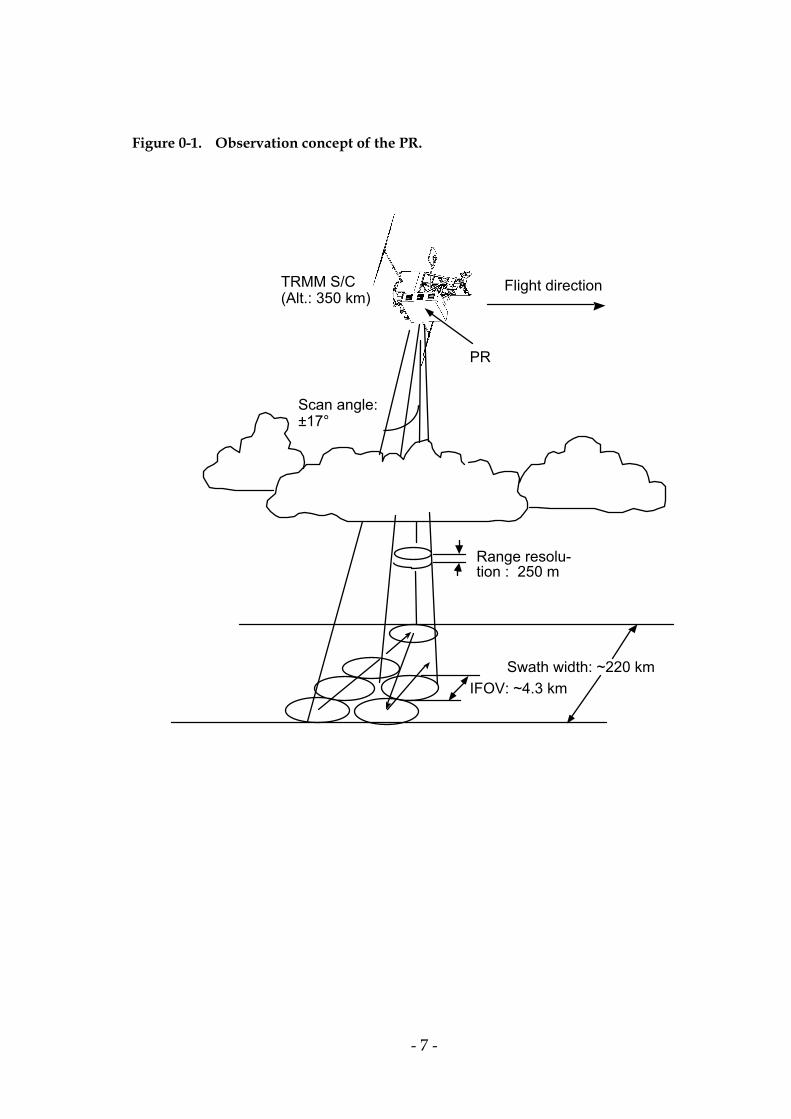
Major design and performance parameters of the PR are shown in Table 0-2 [Kozu et al.,2001]. Observation geometry of PR is shown in Fig 0-1. During the normal observation mode, PR antenna beam scans in the cross-track direction over ±17° to results 220 km swath width from end to end. The antenna beam width of the PR is 0.71° and there are 49 observation angle bins within the scanning angle of ±17°. The horizontal resolution (footprint size) is 4.3 km at nadir and about 5 km at the scan edge when TRMM takes the nominal altitude of 350 km. The range resolution of TRMM PR is 250 m which is equal to the vertical resolution at nadir.
The radar echo sampling is performed over the range gates between the sea surface and the altitude of 15 km for each observation angle bin. For nadir incidence, the “mirror image” is also collected up to the altitude of 5 km. In addition, “oversample ” echo data are partially collected for surface return echoes (for scan angle within ±9.94°) and for rain echoes (for scan angles within ±3.55° up to the height of 7.5 km). These oversampled data will be used for precise measurements of surface return echo level and melting layer structure.
The minimum detectable Z (corresponding to the noise-equivalent received power) improved from 23.3 dBZ (based upon the specifications requirement) to 20.8 dBZ as determined from the pre-launch ground test and from the orbit test. This is mainly due to the increased transmit power and the decrease of the receiver noise figure.

- 2 -
Actually the rain echo power is measured from the subtraction of the system noise power from the total receiver power (rain echo power + system noise power). The accuracy of rain echo power can be characterized by the effective signal-to-noise ratio (S/N), that is the ratio of mean to standard deviation of rain echo power. By considering these facts, the actual minimum detectable Z can be considered to be about 16-18 dBZ after the detailed statistical calculation.The effective signal-to-noise ratio (S/N) of 3 dB is obtained when Z -factor is 17 dBZ. 0-2. TRMM precipitation radar algorithms
The TRMM PR standard algorithms are developed by the TRMM science team. They are classified into Level 1 (1B21, 1C21), Level 2 (2A21, 2A23, 2A25) and Level 3 (3A25, 3A26). Level 1 and Level 2 products are data in the IFOV. Level 3 data give the monthly statistical values of rain parameters mainly in 5° x 5° grid boxes required by the TRMM mission. The characteristics of TRMM PR algorithms are summarized in Table 0-3 where numbers and the names of the algorithms, contact persons, products, and brief descriptions of algorithms are shown. Also the mutual relation of the algorithms are shown in Fig. 0-2.
The algorithm 1B21 produces engineering values of radar received power (signal + noise) and noise levels. It decides whether there exists rain or not in the IFOV. It also estimates the effective storm height from the minimum detectable power value. Algorithm 1C21 gives the radar reflectivity factor, Z, including rain attenuation effects.
The algorithm 2A21 computes the spatial and temporal statistics of the surface scattering coefficient σ0 over ocean or land when no rain is present in the IFOV. Then, when it rains in the IFOV, it estimates the path attenuation of the surface scattering coefficient σ0 by rain using no rain surface scattering coefficient σ0 as a reference [Meneghini, 2000]. The algorithm 2A23 tests whether a bright band exists in rain echoes and determines the bright band height when it exists [Awaka, 1997] .The rain type is classified into the stratiform type, convective type and others by the 2A23. It also detects shallow isolated rain whose height is below the melting level height (zero degree Celsius). The algorithm 2A25 retrieves profiles of the radar reflectivity factor, Z, with rain attenuation correction and rain rate for each radar beam by the combination of Hitschfeld-Bordan and surface reference methods[Iguchi,2000].

- 3 -
As the 13.8 GHz frequency band selected for the TRMM PR is fairly heavily attenuated by rain, the compensation of this rain attenuation becomes the major subject in the rain retrieval algorithms.
Algorithm 3A25 gives the space-time averages of accumulations of 1C21, 2A21, 2A23 and 2A25 products. The most important output products are monthly averaged rain rates over 0.5° x 0.5° and 5° x 5° grid boxes. It also outputs the monthly averaged bright band height over 0.5° x 0.5° and 5° x 5°grid boxes. Algorithm 3A26 gives monthly averaged rain rates over the 5° x 5° grid boxes using the multiple threshold method. 0-3. Altitude change of the satellite and modification of algorithms
The TRMM satellite changed its altitude from 350 km to 402.5 km in August 2001 in order to save the fuel for altitude maintenance. Major impacts of the attitude change (hereafter boost) on the PR are 1) degradation of sensitivity by about 1.2 dB and 2) occurrence of mismatch between transmission and reception angles for one pulse among 32 onboard averaging pulses. The correction algorithm for the latter was added in 1B21 algorithm (please see Chapter 1 for detail). Other than the 1B21, algorithms were not changed according to the altitude change of the satellite. 0-4. On this instruction manual of TRMM PR
The file content description for level 2 and 3 algorithms can be found in the Interface Control Specification (ICS) between the Tropical Rainfall Measuring Mission Science Data and Information System (TSDIS) and the TSDIS Science User (TSU) Volume 4: File Specification for TSDIS Products-Level 2 and 3 File Specifications. It is available at: http://tsdis02.nascom.nasa.gov/
PR team would like to express its sincere gratitude to Ms. Hiraki of JAXA for her help with editing this manual.

- 4 -
0-5. References J. Awaka, T. Iguchi, H, Kumagai and K. Okamoto [1997], “Rain type classification algorithm for TRMM precipitation radar,” Proceedings of the IEEE 1997 International Geoscience and Remote Sensing Symposium, August 3-8, Singapore, pp. 1636-1638. R. Meneghini, T. Iguchi, T. Kozu, L. Liao, K. Okamoto, J. A. Jones and J. Kwiatkowski [2000], “Use of the surface reference technique for path attenuation estimates from the TRMM precipitation radar,” J. Appl. Meteor., 39, 2053-2070. K. Okamoto, T. Iguchi, T. Kozu, H. Kumagai, J. Awaka, and R. Meneghini [1998], “Early results from the precipitation radar on the Tropical Rainfall Measuring Mission,” Proc. CLIMPARA’98, April 27-29, Ottawa, pp. 45-52. T. Iguchi, T. Kozu, R. Meneghini, J. Awaka, and K. Okamoto [2000], Rain-profiling algorithm for the TRMM precipitation radar, J. Appl. Meteor., 39, 2038-2052. T. Kozu, T. Kawanishi, H. Kuroiwa, M. Kojima, K. Oikawa, H. Kumagai, K. Okamoto, M. Okumura, H. Nakatuka, and K. Nishikawa[2001], “Development of Precipitation Radar Onboard the Tropical Rainfall Measuring Mission (TRMM) Satellite,” Proceedings of the IEEE 2001 trans. Geoscience and Remote Sensing, 39, 102-116.
- 5 -
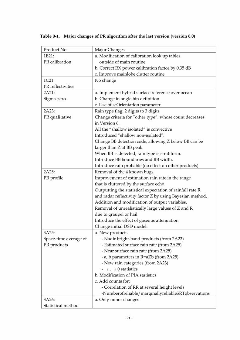
Table 0-1. Major changes of PR algorithm after the last version (version 6.0)
Product No Major Changes 1B21: PR calibration
a. Modification of calibration look up tables outside of main routine b. Correct RX power calibration factor by 0.35 dB c. Improve mainlobe clutter routine
1C21: PR reflectivities
No change
2A21: Sigma-zero
a. Implement hybrid surface reference over ocean b. Change in angle bin definition c. Use of scOrientation parameter
2A23: PR qualitative
Rain type flag: 2 digits to 3 digits Change criteria for “other type”, whose count decreases in Version 6. All the “shallow isolated” is convective Introduced “shallow non-isolated”. Change BB detection code, allowing Z below BB can be larger than Z at BB peak. When BB is detected, rain type is stratiform. Introduce BB boundaries and BB width. Introduce rain probable (no effect on other products)
2A25: PR profile
Removal of the 4 known bugs. Improvement of estimation rain rate in the range that is cluttered by the surface echo. Outputting the statistical expectation of rainfall rate R and radar reflectivity factor Z by using Bayesian method. Addition and modification of output variables. Removal of unrealistically large values of Z and R due to graupel or hail Introduce the effect of gaseous attenuation. Change initial DSD model.
3A25: Space-time average of PR products
a. New products: - Nadir bright-band products (from 2A23) - Estimated surface rain rate (from 2A25) - Near surface rain rate (from 2A25) - a, b parameters in R=aZb (from 2A25) - New rain categories (from 2A23) - ε, ε0 statistics b. Modification of PIA statistics c. Add counts for: - Correlation of RR at several height levels -Numberofreliable/marginallyreliableSRTobservations
3A26: Statistical method
a. Only minor changes

- 6 -
Table 0-2. Major parameters of TRMM PR
Item Specification Frequency Sensitivity Swath width Observable range Horizontal resolution Vertical resolution Antenna Type Beam width Aperture Scan angle Transmitter/receiver Type Peak power Pulse width PRF Dynamic range Number of indep. samples Data rate Mass Power
13.796, 13.802 GHz ≤ ≈ 0.7 mm/h (S/N /pulse ≈ 0 dB) 220 km (from end to end) Surface to 15 km altitude 4.3 km (nadir) 0.25 km (nadir) 128-element WG Planar array 0.71° x 0.71° 2.0 m x 2.0 m ± 17° (Cross track scan) SSPA & LNA (128 channels.) ≥ 500 W (at antenna input) 1.6 µs x 2 ch. (Transmitted pulse) 2776 Hz ≥ 70 dB 64 93.2 kbps 465 kg 250 W
- 7 -
Figure 0-1. Observation concept of the PR.
Scan angle: ±17°
Range resolu-tion : 250 m
IFOV: ~4.3 kmSwath width: ~220 km
TRMM S/C (Alt.: 350 km)
PR
Flight direction
- 8 -
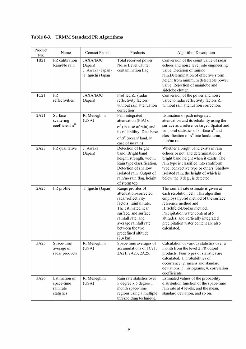
Table 0-3. TRMM Standard PR Algorithms
Product No. Name Contact Person Products Algorithm Description
1B21 PR calibration Rain/No rain
JAXA/EOC (Japan) J. Awaka (Japan)T. Iguchi (Japan)
Total received power, Noise Level Clutter contamination flag.
Conversion of the count value of radar echoes and noise level into engineering value. Decision of rain/no rain.Determination of effective storm height from minimum detectable power value. Rejection of mainlobe and sidelobe clutter.
1C21 PR reflectivities
JAXA/EOC (Japan)
Profiled Zm (radar reflectivity factors without rain attenuation correction).
Conversion of the power and noise value to radar reflectivity factors Zm without rain attenuation correction.
2A21 Surface scattering coefficient σ0
R. Meneghini (USA)
Path integrated attenuation (PIA) of σ0 (in case of rain) and its reliablility. Data base of σ0 (ocean/ land, in case of no rain)
Estimation of path integrated attenuation and its reliability using the surface as a reference target. Spatial and temporal statistics of surface σ0 and classification of σ0 into land/ocean, rain/no rain.
2A23 PR qualitative J. Awaka (Japan)
Detection of bright band, Bright band height, strength, width, Rain type classification, Detection of shallow isolated rain. Output of rain/no rain flag, height of storm top.
Whether a bright band exists in rain echoes or not, and determination of bright band height when it exists. The rain type is classified into stratiform type, convective type or others. Shallow isolated rain, the height of which is below the 0 deg., is detected.
2A25 PR profile T. Iguchi (Japan) Range profiles of attenuation-corrected radar reflectivity factors, rainfall rate. The estimated near surface, and surface rainfall rate, and average rainfall rate between the two predefined altitude (2,4 km).
The rainfall rate estimate is given at each resolution cell. This algorithm employs hybrid method of the surface reference method and Hitschfeld-Bordan method. Precipitation water content at 5 altitudes, and vertically integrated precipitation water content are also calculated.
3A25 Space-time average of radar products
R. Meneghini (USA)
Space-time averages of accumulations of 1C21, 2A21, 2A23, 2A25.
Calculation of various statistics over a month from the level 2 PR output products. Four types of statistics are calculated. 1. probabilities of occurrence, 2. means and standard deviations, 3. histograms, 4. correlation coefficients.
3A26 Estimation of space-time rain rate statistics
R. Meneghini (USA)
Rain rate statistics over 5 degree x 5 degree 1 month space-time regions using a multiple thresholding technique.
Estimated values of the probability distribution function of the space-time rain rate at 4 levels, and the mean, standard deviation, and so on.

- 9 -
Figure 0-2. TRMM Precipitation Radar Algorithm Flow.
TRMM PrecipitationRadar StandardAlgorithm Flow
Level 0Unprocessed Instrument Data
1B21Calibrated Received Power
1C21Radar Reflectivity(Z-factor)
2A253-D Rain Profile(Z, Rain Rate)
2A21
Rain Attenuation
Surface Sigma-02A23PR Qualitative(Rain Type, BB)
3A25Monthly Statisticsof PR Products
3A26Space-Time Averagesusing Threshold Method

- 10 -
1. Level 1 1-1. 1B21: PR received power, 1C21: PR radar reflectivity 1-1. 1. Algorithm Overview The 1B21 calculates the received power at the PR receiver input point from the Level-0 count value which is linearly proportional to the logarithm of the PR receiver output power in most received power levels. To convert the count value to the input power of the receiver, internal calibration data is used. The relationship between the count value and the input power is determined by the system model and the temperature in the PR. This relationship is periodically measured using an internal calibration loop for the IF unit and the later receiver stages. To make an absolute calibration, an Active Radar Calibrator (ARC) is placed at Kansai Branch of NICT and the overall system gain of the PR is being measured nearly every 2 months. Based on the data from the internal and external calibrations, the PR received power is obtained. Note that the calculation assumes that the signal follows the Rayleigh fading, so if the fading characteristics of a scatter are different, a small bias error may occur (within 1 or 2 dB). The other ancillary data in 1B21 include: - Locations of Earth surface and surface clutter (range bin number). Those are useful to identify whether the echo is rain or surface. - System noise level: Four range bins data per angle bin. This is the reference noise floor which is used to extract echo power from the "total" received power in 1B21 (echo + noise). - Oversample data: In order to improve the accuracy of surface echo measurement, and to obtain a better vertical rain profile, 125-m intervals data are available at near-nadir angle bins for rainoversample (up to 7.5 km) and ±10 deg. scan angles for surfaceoversample. - Minimum echo flag: A measure of the existence of rain within a beam. There are multiple confidence levels and users may select up to what confidence level they treat as rain. - Bin storm height: The maximum height at which an echo exists for a specific angle bin. - Land/ocean flag and Topographic height

- 11 -
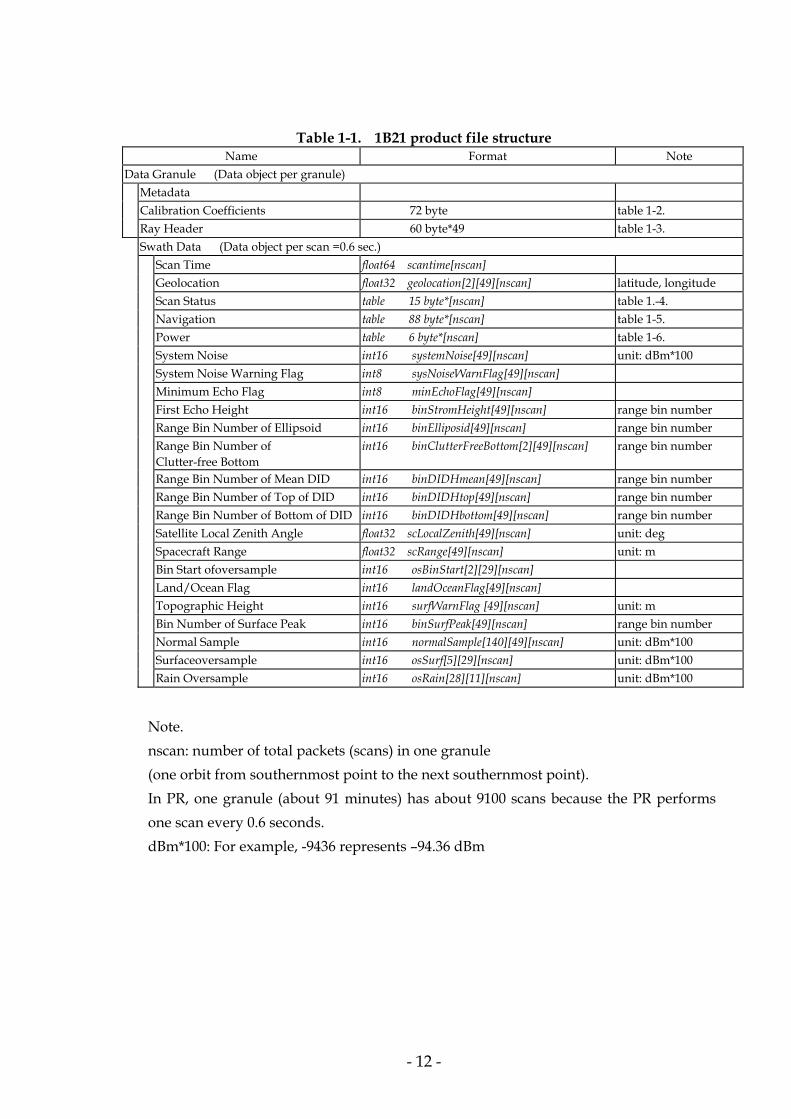
The 1C21 calculates the effective radar reflectivity factor at 13.8 GHz (Zm) without any correction of propagation loss (due to rain or any other atmospheric gas). Therefore, the Zm value can be calculated just by applying a radar equation for volume scatter with PR system parameters. The noise-equivalent Zm is about 21 dBZ. Through the subtraction of the system noise, the Zm value as small as 16 or 18 dBZ are still usable although the data quality is marginal. In 1C21, all echoes stored in 1B21 are converted to "dBZ" unit. This is not relevant for "non-rain" echo; however, this policy is adopted so that the 1B21 and 1C21 product format should be as close as possible except for the following points: - Radar quantity is Zm in dBZ unit instead of received power (dBm). - Data at echo-free range bins judged in 1B21 are replaced with a dummy value. 1-1. 2. File Format 1-1.2.1. 1B21 PRODUCT FILE The main output of the Tropical Rainfall Measurement Mission (TRMM) /Precipitation Radar (PR) Level-1B product, 1B21 is “PR received power.” The file name convention at JAXA EOC is as follows: T1PRYYYYMMDDnnnnn_1B21F00vv.01 PR1B21.YYYYMMDD.nnnnn YYYYMMDD: Observation Date, nnnnn: granule ID, vv: product version number The PR1B21 product is written in Hierarchical Data Format (HDF). HDF was developed by the U.S. National Center for Supercomputing Applications (NCSA). HDF manuals and software tools are available via anonymous ftp at ftp.ncsa. uiuc.edu. The file structure of 1B21 products is shown in Table 1-1.
- 12 -
Table 1-1. 1B21 product file structure Name Format Note Data Granule (Data object per granule) Metadata Calibration Coefficients 72 byte table 1-2. Ray Header 60 byte*49 table 1-3. Swath Data (Data object per scan =0.6 sec.) Scan Time float64 scantime[nscan] Geolocation float32 geolocation[2][49][nscan] latitude, longitude Scan Status table 15 byte*[nscan] table 1.-4. Navigation table 88 byte*[nscan] table 1-5. Power table 6 byte*[nscan] table 1-6. System Noise int16 systemNoise[49][nscan] unit: dBm*100 System Noise Warning Flag int8 sysNoiseWarnFlag[49][nscan] Minimum Echo Flag int8 minEchoFlag[49][nscan] First Echo Height int16 binStromHeight[49][nscan] range bin number Range Bin Number of Ellipsoid int16 binElliposid[49][nscan] range bin number Range Bin Number of
Clutter-free Bottom int16 binClutterFreeBottom[2][49][nscan] range bin number
Range Bin Number of Mean DID int16 binDIDHmean[49][nscan] range bin number Range Bin Number of Top of DID int16 binDIDHtop[49][nscan] range bin number Range Bin Number of Bottom of DID int16 binDIDHbottom[49][nscan] range bin number Satellite Local Zenith Angle float32 scLocalZenith[49][nscan] unit: deg Spacecraft Range float32 scRange[49][nscan] unit: m Bin Start ofoversample int16 osBinStart[2][29][nscan] Land/Ocean Flag int16 landOceanFlag[49][nscan] Topographic Height int16 surfWarnFlag [49][nscan] unit: m Bin Number of Surface Peak int16 binSurfPeak[49][nscan] range bin number Normal Sample int16 normalSample[140][49][nscan] unit: dBm*100 Surfaceoversample int16 osSurf[5][29][nscan] unit: dBm*100 Rain Oversample int16 osRain[28][11][nscan] unit: dBm*100
Note. nscan: number of total packets (scans) in one granule (one orbit from southernmost point to the next southernmost point). In PR, one granule (about 91 minutes) has about 9100 scans because the PR performs one scan every 0.6 seconds. dBm*100: For example, -9436 represents –94.36 dBm

- 13 -
1. Metadata (CoreMetadata.0, ArchiveMetadata.0) Metadata are defined as the inventory information of the TRMM data. EOSDIS 1 has divided the metadata elements into two types: core metadata (EOSDIS Core System (ECS) metadata; CoreMetadata.0) and product-specific metadata (ArchiveMetadata.0). Core metadata are common to most Earth Observing System (EOS2) data products. Product-specific metadata include the specific information of each product. The detailed information is provided in the Appendix. 2. Calibration Coefficients (PR_CAL_COEF) Calibration coefficients consist of several parameters describing the PR electronic performance. They are controlled by JAXA based on the results of PR calibration data analysis. These coefficients are applied in 1B21 (PR received power) calculations.
Table 1-2. Calibration coefficients
Name Format Note
Transmitter gain correction factor float32 transCoef Receiver gain correction factor float32 receptCoef LOGAMP Input/Output characteristics float32 fcifIOchar[16]
The power level at the IF unit corresponding to the count value is calculated by a look-up table which represents input to output characteristics of the IF unit measured by internal calibrations. PR received power is then calculated from this power level and the receiver gain at RF stage.
1 EOSDIS: EOS Data and Information System (NASA) 2 EOS: Earth Observing System (NASA)

- 14 -
3. Ray Header (RAY_HEADER) The Ray Header contains information that is constant in the granule, such as the parameters used in the radar equation, the parameters in the minimum echo test, and the sample start range bin number. These parameters are provided for each angle bin.
Table 1-3. Ray Header
Notes:
a) The Precipitation Radar (PR) has 400 internal (logical) range bins (A/D sample
points) and records “normal sample data (normalSample)” every other range bin from “Ray Start (RayStart)” in order to sample radar echoes from 0-km (the reference ellipsoid surface) to 15-km height.
Name Format Note Ray Start int16 rayStart[49] range bin number of
starting normal sample, see Note (a)
Ray Size int16 raySize[49] number of normal samples in 1 angle see Note (a)
Scan Angle float32 angle[49] unit deg, see Note (b) Starting Bin Distance float32 startBinDist[49] distance (m) between
the satellite and the starting bin sample. unit m, see Note (c)
Rain Threshold #1 float32 rainThres1[49] see Note (d) Rain Threshold #2 float32 rainThres2[49] see Note (d) Transmitter Antenna Gain float32 transAntenna[49] unit: dB Receiver Antenna Gain float32 recvAntenna[49] unit: dB One-way 3dB Along-track Beam Width
float32 onewayAlongTrack[49] unit: rad, see Note (e)
One-way 3dB Cross-track Beam Width
float32 onewayCrossTrack[49] unit: rad, see Note (e)
Equivalent Wavelength float32 eqvWavelength[49] unit: m, see Note (f) Radar Constant float32 radarConst[49] unit: dB, see Note (g) PR Internal Delayed Time float32 prIntrDelay[49] set to 0 Range Bin Size float32 rangeBinSize[49] unit: m, see Note (a), (h) Logarithmic Averaging Offset float32 logAveOffset[49] unit: dB, see Note (i) Main Lobe Clutter Edge int8 mainlobeEdge[49] see Note (j) Side Lobe Clutter Range int8 sidelobeRange[3][49] see Note (k)

- 15 -
The number of recorded samples at an angle bin depends on the scan angle and is defined by “Ray Size (RaySize).” The N-th normal sample data can be converted to the internal logical range bin number as follows;
Logical range bin number at N-th normal sample
= RayStart + )1(2 −× N b) Scan Angle (angle) is defined as the cross-track angle at the radar electric
coordinates which are rotated by 4 degrees about the Y-axis (Pitch) of spacecraft coordinates.*3 The angle is positive when the antenna beam is rotated counter clockwise (CCW) from the nadir about the +X axis of the radar electric coordinates.
c) Starting Bin Distance is determined by the sampling timing of the PR. The
distance between the satellite and the center of the N-th normal sample bin is calculated as follows:
Distance = “Starting Bin Distance (startBinDist)” + “Range Bin Size (rangeBinSize)” )1( −× N
This distance is defined as the center of a radar resolution volume which extends ± 125 m . d) Rain Thresholds (rainThres1 and rainThres2) are used in the minimum echo
test. e) Beam widths, both along track beam width and cross track beam width
(onewayAlongTrack and onewayAcrossTrack), are recorded based on the fact that the PR main beam is assumed to have a two-dimensional Gausian beam pattern.
f) “Euivalent Wavelength (eqvWavelength)” = 2c f1 + f2( ) where c is the speed of light, and f1 and f2 are PR’s two frequencies.
3 If there is no attitude error, +X (or sometimes –X, see Spacecraft Orientation in Scan Status) is along the spacecraft flight direction, +Z is along the local nadir, and +Y is defined so that the coordinates become a right-hand Cartesian system.

- 16 -
g) Radar Constant (radarConst) is defined as follows, and is used in the radar
equation:
= −18
10
23
0 10ln22
K10logC π
( ) ( )2/ +−= ε1εK
ε : the relative dielectric constant of water K 2 = 0.9255
K 2 is the calculated value at 13.8 GHz and 0 degree C based on Ray (1972).*
4 With this constant, users can convert from PR receiving
powers to rain reflectivity. (See the 1C products.) h) Range Bin Size (rangeBinSize) is the PR range resolution and is the width at
which pulse electric power decreases 6dB (-6 dB width). i) Logarithmic Averaging Offset (logAveOffset) is the offset value between the
logarithmic average and the power-linear average. The PR outputs the data of 1 range bin which is the average of 64 LOGAMP outputs. “Received power” in the PR1B21 output is corrected for the bias error caused by the logarithmic average and is thus equal to normal average power.
j) Main Lobe Clutter Edge (mainlobeEdge) is a parameter previously used as the
lowest range bin for the minimum echo test. This is the absolute value of the difference in range bin number between the surface peak and the edge of the clutter from the main lobe.
k) Absolute value of the difference in Range bin numbers between the bin
number of the surface peak and the possible clutter position. A maximum of three range bins can be allocated as "possible" clutter locations. “Zero” indicates no clutter.
Note: Items j) and k) are not useful for detailed examination of radar echo range profile, especially over land. Please refer to 14 (“Range Bin Number of Clutter-free Bottom”), 23 “Bin Number of Surface Peak” and so on.
4 Ray, P.S., 1972: Broadband complex refractive indices of ice and water. Appl.Opt., Vol.11, No.8, 1836-1844.
- 17 -
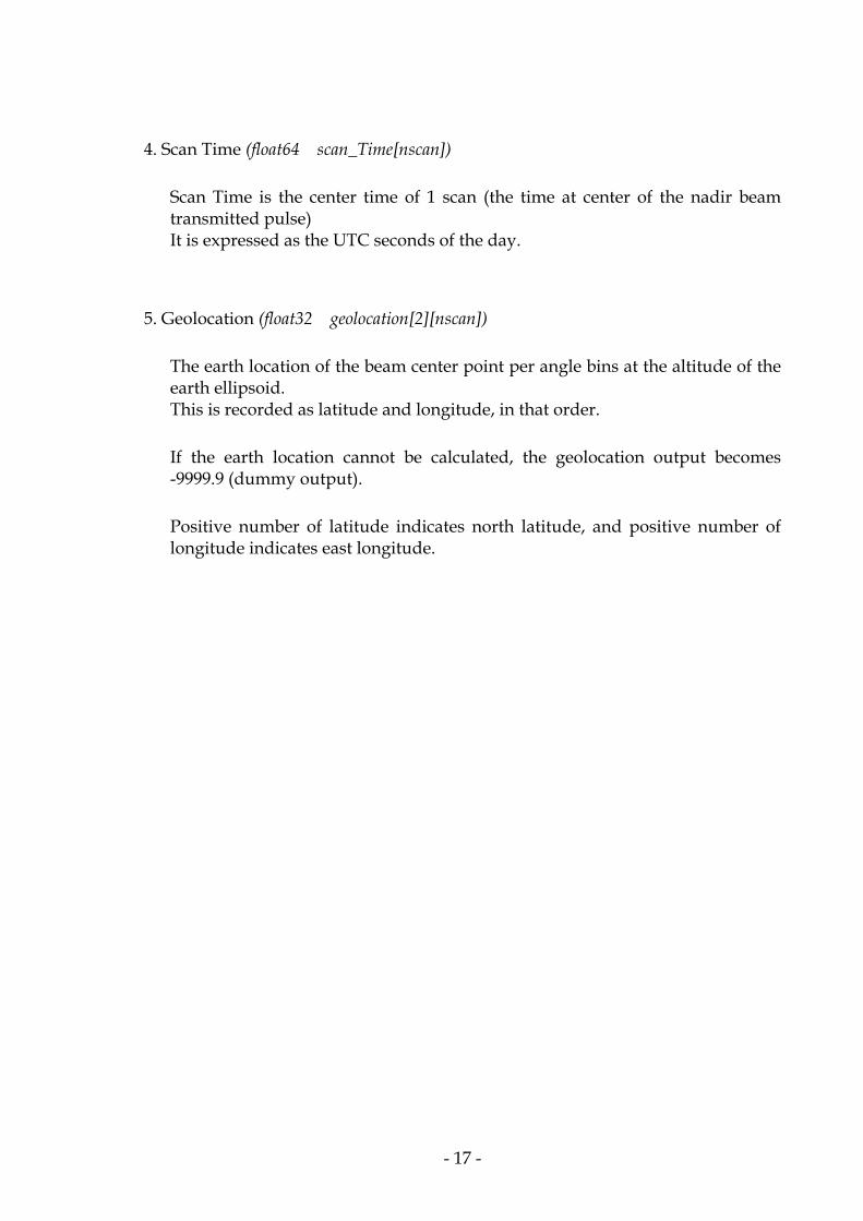
4. Scan Time (float64 scan_Time[nscan])
Scan Time is the center time of 1 scan (the time at center of the nadir beam transmitted pulse) It is expressed as the UTC seconds of the day.
5. Geolocation (float32 geolocation[2][nscan])
The earth location of the beam center point per angle bins at the altitude of the earth ellipsoid. This is recorded as latitude and longitude, in that order.
If the earth location cannot be calculated, the geolocation output becomes -9999.9 (dummy output).
Positive number of latitude indicates north latitude, and positive number of longitude indicates east longitude.

- 18 -
6. Scan Status (pr_scan_status[nscan]) The status of each scan, that is, quality flags of spacecraft and instrument, are stored.
Table 1-4. Scan Status Name Format Note
Missing int8 missing The values are: 0: normal 1: missing (missing packet and calibration mode) 2: No-rain
Validity 8-bit validity The summary of operation mode. If all items are normal, zero is recorded. Bit meaning if bit=1 <bit1>: Non-routine spacecraft orientation (2 or 3 or 4) <2>: Non-routine ACS mode (other than 4) <3>: Non-routine yaw update status (0 or 1) <4>: PR operation mode (other than 1) <5>: Non-routine QAC (QAC bit 2, 6 or 7 is not zero)
QAC 8-bit qac Quality information regarding demodulation status at Level-0 processing (quality accounting capsule) <bit1>: RS header error <2>: Data unit length code wrong <3>: RS frame error <4>: CRC frame error <5>: Data unit sequence count error <6>: Detected frame error during generation of this data unit <7>: Data unit contains fill data
Geolocation Quality
8-bit geoQuality Bit meaning if bit =1 <0>: latitude limit error <1>: geolocation discontinuity <2>: attitude change rate limit error <3>: attitude limit error <4>: maneuver <5>: using the predictive orbit data <6>: geolocation calculation error If geolocation quality is not zero, the geolocation accuracy is not assured.
Data Quality 8-bit dataQuality Total summary of scan data. If this is not zero, the data is not processed in 1C. Bit meaning if bit =1 <0>=1: Missing (No data) <5>=1: Bad Geolocation Quality <6>=1: Bad Validity
Spacecraft Orientation
int8 scOrient The information in spacecraft Attitude Control System. Value 0 and 1 is normal. Value Meaning 0:+x forward 1:-x forward 2:-y forward 3:CERES calibration

- 19 -
4:Unknown orientation ACS mode int8 acsMode The mode of spacecraft Attitude Control System.
Value: Meaning 0: stand-by 1: Sun acquire 2: Earth acquire 3: Yaw acquire 4: Normal 5: Yaw maneuver 6: Delta-H (Thruster) 7: Delta-V (Thruster) 8: CERES Calibration
Yaw Update Status
int8 yawUpdateS The information in spacecraft Attitude control system. Value: Meaning 0: inaccurate 1: indeterminate 2: accurate
PR Mode int8 prMode
Value: Meaning 0: other mode 1: Observation mode
PR status #1 8-bit prStatus1 Bit meaning if bit =1 <0>: LOGAMP noise limit error <1>: Noise level limit error <2>: Out of PR dynamic range <3>: Not reach surface position <7>: FCIF mode change (see 1.27)
PR status #2 8-bit prStatus2 Bit meaning if bit =1 <0> Warning for clutter because of strong
nadir surface echo. (see 1.28) Fractional Orbit Number
float32 fracOrbitN The fractional part of the orbit at scan time. (Scan time - Orbit Start Time) / (Orbit End time - Orbit Start Time)
Notes:
MSB LSB · bit number 7 6 5 4 3 2 1 0
a) PR Status #1 in Scan Status
The flags listed here indicate warnings of PR conditions (noise level, echo power and echo position, and mode change). In data processing, users should be cautions with the following as a scan with non-zero status includes questionable range bins or angle bins.
<1> Noise level limit error: The meaning of this warning is the same as
10 ”System Noise Warning Flag”. <2> Surface echo is so strong that it exceeds the PR receiver dynamic
range. If this bit is ON, surface echo level may be questionable. <3> If Surface echo is out of range window, Bin Surface Peak and
related data become uncertain.

- 20 -
b) PR Status #2 in Scan Status In some cases, antenna sidelobes are directed to nadir receive surface echo positions. When the main beam is off nadir, the timing of such nadir-surface clutter can contaminate the rain echo. In “PR STATUS2,” a warning flag is set ON (1) when the nadir surface echo (at the nadir angle bin #25) exceeds a predetermined threshold. When the flag is ON, please be careful about the echoes at all angle bins around the same logical range bin number as the Bin-surface-peak at nadir (angle bin number 25).
7. Navigation (pr_navigation) This is the output of NASA’s geolocation toolkit. This is recorded each angle.
Table 1-5. Navigation Name Format Note
X component of spacecraft position float32 scPosX unit: m Y component of spacecraft position float32 scPosY unit: m Z component of spacecraft position float32 scPosZ unit: m X component of spacecraft velocity float32 scVelX unit: m/s Y component of spacecraft velocity float32 scVelY unit: m/s Z component of spacecraft velocity float32 scVelZ unit: m/s Spacecraft geodetic latitude float32 scLat Spacecraft geodetic longitude float32 scLon Spacecraft geodetic altitude float32 scAlt unit: m Roll of spacecraft attitude float32 scAttRoll unit: deg Pitch of spacecraft attitude float32 scAttPitch unit: deg Yaw of spacecraft attitude float32 scAttYaw unit: deg Sensor Orientation Matrix #1 float32 att1 Sensor Orientation Matrix #2 float32 att2 Sensor Orientation Matrix #3 float32 att3 Sensor Orientation Matrix #4 float32 att4 Sensor Orientation Matrix #5 float32 att5 Sensor Orientation Matrix #6 float32 att6 Sensor Orientation Matrix #7 float32 att7 Sensor Orientation Matrix #8 float32 att8 Sensor Orientation Matrix #9 float32 att9 Greenwich Hour Angle float32 greenHourAng unit: deg
Notes : a) spacecraft position: The position (in meter) in Geocentric Inertial
Coordinates at the Scan time. These coordinates will be True of Date, as interpolated from the data in NASA flight dynamics facility ephemeris files.
b) sensor orientation matrix: The rotation matrix from the instrument coordinate frame to geocentric inertial coordinate.

- 21 -
8. Power (powers) Power is recorded for each scan and consists of the calibrated PR transmitter power and the transmitter pulse width.
Table 1-6. Power Name Format Note PR transmitter power int16 radarTransPower unit: dBm*100 PR transmitter pulse width float32 transPulseWidth unit: sec
Note: dBm*100: For example, -9436 represents –94.36 dBm 9. System Noise (int16 systemNoise[49][nscan]) System Noise is recorded in each angle bin. This is the value estimated by averaging four noise samples. Unit is dBm*100. The system noise consists of external noise and PR internal noise, and is recorded as the total equivalent noise power at the PR antenna output. If data is missing, the dummy value (-32734) is recorded. 10. System Noise Warning Flag (int8 sysNoiseWarnFlag[49][nscan]) If the system noise level exceeds the noise level limit, the flag is set to 1. This will occur when (1) a radio interference is received, (2) system noise increases anomalously, or (3) noise level exceeds the limit due to the statistical variation of the noise. In cases (1) and (2), data should be used carefully. In case (3), this flag may be neglected. Received power levels in all range bins will increase in cases (1) and (2) as much as the increase of the system noise. PR may receive radio interference in the following areas. N3.1 E 101.7 (in Malaysia) N33.8 W118.2 (around Los Angeles) S34.8 W68.4 (around Santiago) N10.5 W66.9 (in Chili) N4.7 E36.9 (around Ethiopia – Kenya border) S32.8 W63.4 (around Amazon) etc.

- 22 -
11. Minimum Echo Flag (int8 minEchoFlag[49][nscan]) This value shows the esistence of the rain echo at each angle bin. Six values are used in the Minumun Echo Flag: 0, 10, 20, 11, 12, and 13.
0: No rain. (Echoes are very weak.) 10: Rain possible but may be noise. (Some weak echoes above noise
exist in clutter free ranges.) 20: Rain certain. (Some strong echoes above noise exist in clutter
free ranges.) 11: Rain possible but may be noise or surface clutter. (Some weak
echoes exist in possibly cluttered ranges.) 12: Rain possible but may be clutter. (Some strong echoes exist in
possibly cluttered ranges.) 13: Rain possible but probably sidelobe clutter. (Some strong echoes
above noise exist but they are most likely caused by sidelobe clutter, see section 1-4.)
Please be careful using the Minimum Echo Flag except when it is 0 or 20. 12. First Echo Height (int16 binStormHeight[2][49][nscan]) The First Echo Height (storm height) is represented by the logical range bin number (1 to 400, 125-m interval). Two types of First Echo Height are estimated, depending on whether the minimum echo flag = 10 or 20. (If the first echo is detected below the clutter-free bottom, the two types depend on whether the flag = 11 or 12.) 13. Range Bin Number of Ellipsoid (int16 binEllipsoid[49][nscan])
Ellipsoid Height is represented by the logical range bin number (1 to 400). This is calculated by the following equation.
binEllipsoid[j] = RayStart + (scRange – startBinDist)/rangebinSize x 2 (scRange: see 19. spacecraft range)

- 23 -
14. Range Bin Number of Clutter-free Bottom
(int16 binClutterFreeBottom[2][49][nscan]) This is the bottom range-bin number (logical range bin number) in clutter-free range bins estimated by the algorithm provided by Dr. Awaka (Hokkaido Tokai Univ., Japan).
binClutterFreeBottom [0][49]: clutter free certain, binClutterFreeBottom [1][49]: clutter free probable.
15. Range Bin Number of Mean DID (int16 binDIDHmean[49][nscan]) binDIDHmean represents the range bin number corresponding to the mean height of all DID data samples available in a 5× 5km area that overlaps most with the footprint. 16. Range Bin Number of Top of DID (int16 binDIDHtop[49][nscan]) binDIDHtop[][0] represents the range bin number corresponding to the highest value (top) of all DID data samples in a 5× 5km box, and binDIDHtop[][1], the range bin number corresponding to the highest value in a 11× 11km box. 17. Range Bin Number of Bottom of DID (int16 binDIDHbottom[49][nscan]) The definition is the same as that of binDIDHtop[49][2] except that the value represents the lowest value (bottom) of all DID samples in a 5× 5km or 11× 11km box. 18. Satellite Local Zenith Angle (float32 scLocalZenith[49][nscan]) The angle between the local zenith (on the Earth ellipsoid) and the beam center line.

- 24 -
19. Spacecraft Range (float32 scRange[49][nscan])
The distance between the spacecraft and the center of the footprint of the beam on the Earth ellipsoid.
20. Bin start ofoversample (int16 osBinStart[49][nscan]) The first byte indicates that logical range bin number of starting theoversample. The second byte indicates the status of the onboard surface tracker (0, normal; 1, Lock off). Oversample only applies to 29 angles (angle 11 to 39). 21. Land/Ocean Flag (int16 landOcenFlag[49][nscan]) The land or ocean information from the Digital Terrain Elevation Dataset (DTED) Intermittent Dataset (DID) provided by NASA/JPL. 0 = water (ocean or inland water) 1 = land 2 = coast (not water nor land) 3 = water (surface peak is not correctly detected because of high attenuation) 4 = land /coast (surface peak is not correctly detected because of high attenuation) In the product version 6, two categolies are added in the landOceanFlag. The new flags appear when the land (or ocean) surface position is not correctly detected because of high attenuation relating to heavy rainfall. This is determined by the Clutter routine in 1B21. The landOceanFlag is 3 when the surface peak is not detected correctly over ocean. In this case, binSurfPeak is set at binEllipsoid. If the phenomena happened over land or coast, landOceanFlag is 4 and the binSurfPeak is recalculated using data between the binClutterFreeBottom and binClutterFreeBottom+8 (bins) toward the Earth.

- 25 -
22. Topographic Height (int16 surfWarnFlag[49][nscan]) The topographic mean height (m) of all DID samples in a 5× 5km. 23. Bin Number of Surface Peak (int16 binSurfPeak[49][nscan]) The bin surface peak indicates the logical range bin number of the peak surface echo. The algorithm to detect the surface peak is provided by Dr. Kozu, CRL (presently at Shimane Univ.). If the surface is not detected, Bin Surface Peak is set to a value of -9999. Note that the echo peak may appear either in the normal sample data or in the oversample data. 24. Normal Sample (PR received power) (int16 normalSample[140][49][nscan]) The normal sampled PR received powers are recorded (unit: dBm*100). The data is stored in the array of 49 angles ∗ 140 elements. Since each angle has a different number of samples, the elements after the end of sample are filled with a value of -32767. If a scan is missing, the elements are filled with the value -32734. Logical range bin number comparable with binSurfPeak, binEllipsoid, etc. is calculated with rayStart in RAY_HEADER (see 3. Ray Header, Note a ). 25. Surface Oversample (int16 osSurf[5][29][nscan]) The PR records theoversampled data in five range bins around the surface peak detected on board (not Bin Surface Peak) in a total of 29 angle bins (nadir± 14 angles, angle bins 11 to 39) to examine the surface peak precisely (unit: dBm*100). If the surface tracker status is lock-off, the data position is unknown. To use the oversample data, fill the five data starting at “Bin Start of Over_Surface (osBinStart)” in every other logical range bin, then merge with the interleaving normal sample data.

- 26 -
26. Rain Oversample (int16 osRain[28][11][nscan]) The PR records the oversampled data at 28 range bins in a total of 11 angle bins (nadir± 5 angles: angle bins 20 to 30) to record the detailed vertical profile of the rain (unit: dBm*100). The 125m interval dataset in heights from 0 km to 7.5 km can be generated by interleaving the Normal Samples with the Surfaceoversamples and rain oversamples. The data are merged in the same way as the Surface Oversample. The osBinStart expresses the start angle bin of rain oversample for the rain oversample angle bins and the surfaceoversample follows the rain oversample continuously. Therfore, the logical range bin number of the Surfaceoversample and Rain Oversample is as follows: Angle bin 11 – 19, 31-39 : Logical range bin number at Nth surface oversample = osBinStart +2(N-1) Angle bin 20-30: Logical range bin number at Nth rain oversample = osBinStart+2(N-1): Logical range bin number at Nth surface oversample= osBinStart+56+2(N-1) 1-1.2.2. 1C21 PRODUCT FILE The main output of the PR Level-1C, 1C21, is the radar “reflectivity factor.” The file format is exactly the same as that of 1B21 except for the replacement of the received power by the radar reflectivity factor and noise (no echo range bin) by a dummy value.

- 27 -
Table 1-7. 1C21 products file structure Name Format Note
Data Granule (Data object per granule)
Metadata
Calibration Coefficients 72 byte table 1-2.
Ray Header 60 byte*49 table 1-3.
Swath Data (Data object per scan =0.6 sec.)
Scan Time float64 scantime[nscan]
Geolocation float32 geolocation[2][49][nscan] latitude, longitude
Scan Status table 15 byte*[nscan] table 1.-4.
Navigation table 88 byte*[nscan] table 1-5.
Power table 6 byte*[nscan] table 1-6.
System Noise int16 systemNoise[49][nscan] dBm*100
System Noise Warning Flag int8 sysNoiseWarnFlag[49][nscan]
Minimum Echo Flag int8 minEchoFlag[49][nscan]
First Echo Height int16 binStromHeight[49][nscan] range bin number
Range Bin Number of Ellipsoid int16 binElliposid[49][nscan] range bin number
Range Bin Number of Clutter-free
Bottom
int16 binClutterFreeBottom[2][49][nscan] range bin number
Range Bin Number of Mean DID int16 binDIDHmean[49][nscan] range bin number
Range Bin Number of Top of DID int16 binDIDHtop[49][nscan] range bin number
Range Bin Number of Bottom of DID int16 binDIDHbottom[49][nscan] range bin number
Satellite Local Zenith Angle float32 scLocalZenith[49][nscan] deg
Spacecraft Range float32 scRange[49][nscan] m
Bin Start ofoversample int16 osBinStart[2][29][nscan]
Land/Ocean Flag int16 landOceanFlag[49][nscan]
Topographic Height int16 surfWarnFlag [49][nscan] m
Bin Number of Surface Peak int16 binSurfPeak[49][nscan] range bin number
Normal Sample int16 normalSample[140][49][nscan] dBZ*100
Surface Oversample int16 osSurf[5][29][nscan] dBZ*100
Rain Oversample int16 osRain[28][11][nscan] dBZ*100

- 28 -
Notes:For example, -9436 represents –94.36 dBZ The 1C21 product has the same format as 1B-21. In 1C-21, the normal sample, surfaceoversample and rain oversample contain radar reflectivity factors (dBZ, mm6/m3) which are converted from the PR received powers in the corresponding places in 1B21 output. The radar equation used is
Zmrange
1wavelength
pulseccrossalongGrGtPtln22K
Pr(range) 2210
23 ∗∗∗∗∗∗=
π
( ) ( )( ) e)20log(rangC101010logdBZm Pn/10Ps/10 +−−=
Ps: 1B21 received power Pn:1B21 noise level range:Distance
( ) ( ) ( ) 0Cwavelength20logpulsec10logcrossalong10logGrGtPtC +−×+×+++=
Pt: transmitter power (in power) pulse:transmitter pulse width (in power) Gt: transmit antenna gain (in ray header) Gr: receive antenna gain (in ray header) along:Along-track beam width (in ray header) cross:Cross-track beam width (in ray header) c:speed of light wavelength:wave length (in ray header) C0:Radar Constant (in ray header)
If received power is below the noise level, the reflectivity is filled with a dummy value of -32700. *Note that the radar reflectivity factors given in 1C-21 are apparent values and include rain or atomospheric attenuation.

- 29 -
1-1. 3. Changes in 1B21 after the satellite boost in August 2001 1. Outline of the boost The TRMM satellite changed its altitude from 350 km to 402.5 km in August 2001 in order to save the fuel for altitude maintenance. Major impacts of the attitude change (hereafter boost) on the PR are 1) degradation of sensitivity by about 1.2 dB and 2) occurrence of mismatch between transmission and reception angles for one pulse among 32 onboard averaging pulses. The latter causes unknown error of the PR’s data because the mismatch pulse is averaged with other 31- nominal pulses by onboard processor. In order to mitigate the mismatch error in PR data, level one algorithm (1B21) added mismatch correction routine. 2. The mismatch correction algorithm in 1B21 The basic idea of the mismatch correction algorithm is to retrieve the power of mismatch pulse received by PR based on the antenna pattern of mismatch pulse as mentioned previous section. In the current correction algorithm of mismatch in 1B21 algorithm assumes followings: 1) mismatch pulse power can be expressed as the average of power from current angle bin and one previous angle bin with 6 dB gain reduction, 2) the one previous angle bin data can be used without correction to avoid the accumulation of error to the following angle bins, though it contains mismatch error, and 3) the data of angle bin 1 (the first angle bin each scan) contains 31 normal pulse data and one noise data as mentioned in previous section. The correction algorithm is preferred to be expressed by simple equation and be applied for various occasions such as rain echo and surface echo. The equation of mismatch correction in 1B21 algorithm is expressed as where N is angle bin number (angle bin to be corrected), P(N) is observed power at a certain range bin of angle bin N in dBm (containing mismatch echo), P(N-1) is the one previous angle bin data of same distance from the PR used as the “reference”, and Pc(N) is corrected power in dBm. In this equation, since the obtained data is the result from averaging of 32 pulses, 32 times of P(N) stands for the total received power. The estimated correction error is less than 0.2 dB for rain echo and less than 0.3 dB
( ) ( )( ) ( )
3162101010log1032
10/110/
+
+⋅−⋅=
−NPNPNPNPc

- 30 -
for surface echo. 1-1. 4. Major changes in 1B21 algorithm for product version 6 1. Improvement of surface peak range bin number detection algorithm. This routine is for the cases that the surface echo is fully attenuated by strong rainfall. In this case, surface peak is searched again using the output from clutter routine by Dr. Awaka. For the case of ocean, binSurfPeak is replaced by binEllipsoid. 2. Refurbishment of calibration table Discontinuity between linear fitting part and parabolic fitting part should be corrected. Modification of calibration table in order to be applicable to the data around December 15, 1997, when the NASDA performed initial check out of PR by changing internal attenuation for various values. 3. Correction for a known error in the receiver calibration factor It should be about -1.0 dB instead of -0.65dB.(input for 1B21) 1-1. 5. Comments on PR Level 1 products 1. Calibration accuracy The TRMM Precipitation Radar (PR) has been working without any problem since the first turn-on of the PR power in the beginning of December 1997. The initial checkout of the PR was completed by NASDA and CRL at the end of January 1998. The overall calibration of the PR including the transmit and receiving antenna pattern measurements were made by using an ARC. It was concluded that the ARC calibration results are reasonable and consistent with the corresponding values calculated by using the PR system parameters. Also the ocean surface sigma-0 obtained by the PR has been found to be quite consistent with those observed from previous airborne and satelliteborne scatterometers.

- 31 -
2. Sensitivity The minimum detectable Zm (corresponding to the noise-equivalent received power) improved from 23.3 dBZ (based upon the specifications requirement) to 20.8 dBZ as determined from the pre-launch ground test and from the orbit test. This is mainly due to the increased transmit power and the decrease of the receiver noise figure. Actually the rain echo power is measured from the subtraction of the system noise power from the total receiver power (rain echo power + system noise power). The accuracy of rain echo power can be characterized by the effective signal-to-noise ratio (S/N), that is the ratio of mean to standard deviation of rain echo power. By considering these facts, the actual minimum detectable Zm can be considered to be about 16-18 dBZ after the detailed statistical calculation. The effective signal-to-noise ratio (S/N) of 3 dB is obtained when Zm is 17 dBZ. 3. Discrimination of rain from surface clutter It is generally very difficult to discriminate rain echo from surface clutter especially in mountainous regions. An algorithm has been implemented which analyzes the radar echo range profile very carefully to determine the boundary between rain and surface echoes. The result has been reflected into the surface location related variables described in Item 6. Even though, there is a very small possibility that a surface echo is treated as a rain echo (and in mountainous regions, clutter position when it rains can happen to become too high in a very rare occasion). Please be careful when you use the PR Level-2 data to study rain structure in mountainous regions. Strong echoes near the surface are likely surface clutter and should be excluded from rain analysis.

- 32 -
4. Surface clutter from the coupling between nadir-direction antenna sidelobe and strong surface radar cross-section (NRCS) It has been found that the echo strength from nadir direction is sometimes extremely strong, which exceeds the anticipated value in the PR design. This seems to occur wet and flat land areas rather than ocean. Even dry dessert regions, the NRCS seems very strong in some cases. In such cases antenna sidelobes directed to nadir receive surface echoes. When main beam is off-nadir, the timing of such nadir-surface clutter can contaminate the rain echo. In "PR STATUS2", a warning flag is set ON when the nadir surface echo (at the nadir angle bin, #25) exceeds a pre-determined threshold. When it is ON, please be careful about the echoes in all angle bins at the same range bin number as the Bin_surface_peak (binSurfPeak) at nadir (angel bin number 25). 5. Discrimination of rain echo from noise In order to help users utilization of the data, the 1B21 product contains the "Minimum Echo Flag" which indicates the existence of rain in the clutter free range or in the clutter range. Since thermal noise, rain echo and resulting thermal noise plus rain echo follow Rayleigh fading, the PR received echo is a result of the averaging 64 number of independent samples. The averaged value still has small fluctuations of about 0.7 dB to 1 dB, depending on signal-to-noise ratio. In order not to miss weak echo which is sometimes useful to study rain structure, etc, the threshold to set the flag = rain possible is currently about 90% value of the cumulative distribution of thermal noise. This means quite a large fraction of data having "rain possible" flag is only thermal noise. Since this rain/no-rain discrimination is sometimes affected by the surface clutter at especially mountainous area. In the clutter region, rain/no-rain discrimination often misidentifies clutter as rain.
Minimum Echo Flag includes clutter flag. There are five levels in the Minimum Echo Flag; 0, 10, 20, 11, and 12:
0 = no rain (Echoes are very weak), 10 = rain possible but maybe noise (Some weak echoes above noise exist in clutter free ranges), 20 = rain certain (Some strong echoes above noise exist in clutter free ranges),

- 33 -
11 = rain possible but maybe noise or surface clutter (Some weak echoes exist in possibly cluttered ranges), and rain possible but maybe clutter 12 = (Some strong echoes exist in possibly cluttered ranges).
Therefore please be careful in using the Minimum Echo Flag except 0 and 20.
6. Information concerning the surface location in 1B21 and 1C21. The following variables are newly added in 1B21 and 1C21 products. a. Range bin number of Ellipsoid (binEllipsoid) b. Range bin number of clutter free bottom (binClutterFreeBottom) c. Range bin number of mean DID (binDIDHmean) d. Range bin number of top of DID (binDIDHtop) e. Range bin number of bottom of DID (binDIDHbottom) As you can imagine from the name of each variable, those represent range bin numbers corresponding to the surface height from the Earth ellipsoid, which may be useful to analyze a range profile of PR received power or radar reflectivity factor. 7. Bin_surface_peak (binSurfPeak) and oversample data In PR 1B21, the data called Bin_surface_peak indicates the range bin number at which PR received power has the maximum within a range window centered at the range bin number determined from a Digital Elevation Model (DID). In most cases, the Bin_Surface_Peak gives the correct location corresponding to the location of actual surface. There may be small number of cases where Bin_surface_peak is wrong. One possibility a case in which DID is in error, and the other is a case in which rain echo is so strong so that surface echo is masked by the rain echo. We expect those cases are rare, but please keep in mind those may occur with a small probability.

- 34 -
The oversample data are recorded onboard based on the location of surface echo peak detected by an onboard surface tracking function. Since this tracker may be locked-off in mountainous regions, there are cases in whichoversample data are recorded outside the location of surface echo. In such cases the oversample data may not be useful because it may not be used for improving the accuracy of surface echo power or for detailed study of vertical storm structure. The difference between the location of surface echo estimated by the onboard tracker (Note 1) and Bin_surface_peak is a measure of the goodness of oversample data in terms of its covering region in the radar range profile.
Note 1: The surface echo location estimated onboard (Y) can be obtained from
"Bin_start_oversample(osbinStart)"data.
Let X be Bin_start_oversample, Y = X + 60 or + 61 (angle bins between 20 and 30) and Y = X + 4 or +5 (between 11 and 19 and between 31 to 39). We cannot judge either 60 or 61 (or 4 or 5) from 1B21 itself, however.
8. Interference from other radio services around 13-14 GHz There have been several cases where PR suffered from interferences from other radio services, mainly from satellite tracking and control stations using 13-14 GHz bands. The probability is very small, and the impact to TRMM mission appears to be negligible. In a typical interference case, the noise level increases a few to several decibels over entire range bins for a very short period (one or two scans). In such a case, PR sensitivity to detect weak echo is degraded accordingly.

- 35 -
1-1. 6. Planned Improvements Routine monitoring of PR performance and periodical ARC calibrations are being conducted. Depending on the drift of PR system parameters, the calibration factors and the look-up table may be updated in future. 1-1. 7. References T. Kozu, T. Kawanishi, K. Oshimura, M. Satake, H. Kumagai; TRMM precipitation radar: calibration and data collection strategies, Proc. IGARSS'94, 2215-2217, Pasadena, 1994. M. Satake, K. Oshimura, Y. Ishido, S. Kawase, T. Kozu: TRMM PR data processing and calibration to be performed by NASDA, Proc. IGARSS'95, 426-428, Florence, 1995. N. Takahashi and T. Iguchi; Estimation and correction of beam mismatch of the precipitation radar after an orbit boot of the Tropical Rainfall Measuring Mission satellite, IEEE Trans. Geo. and Remote Sens., 42, 2362-2369, 2004.

- 36 -
1-2. DID access routine 1-2. 1. Objectives A DID access routine is used in a Level-1 PR algorithm, 1B21. Main objectives of the DID access routine are:
(a) To output the elevation information over a 5 km * 5 km box and an 11 km * 11 km box using DID elevation data, with the center for the 5 km * 5 km box being the same as the center for the 11 km * 11 km box.
(b) To output the land/water information over a 5 km * 5 km box, which is the same as the 5 km * 5 km box for (a), using DID land/water data.
Note: DID stands for DTED (Digital Terrain Elevation Dataset) Intermediate Dataset.
1-2. 2. Method used
(a) Conversion of DID data having 1 km horizontal resolution to a 5 km * 5 km box and an 11 km * 11 km box.
1-2. 3. Flowchart
Opening of DID file
Clear cache memory when the memory is full
Access 49 angle bins of data at one time
Conversion to 5km * 5km box and 11km * 11km box data
Closing of DID file

- 37 -
1-2. 4. Some details of the algorithm
(a) Height_mean A mean of DID elevation over a 5 km * 5km box, Height_mean, is computed with the following weights:
0.014, 0.028, 0.034, 0.028, 0.014, 0.028, 0.055, 0.069, 0.055, 0.028, 0.034, 0.069, 0.088, 0.069, 0.034, 0.028, 0.055, 0.069, 0.055, 0.028, 0.014, 0.028, 0.034, 0.028, 0.014.
(b) Land/water flag
The original land/water information having 7 categories is summarized into the following information over the 5 km * 5 km box with 3 categories:
(1) water if the 5 km * 5 km box has the following categories of data only,
- deep ocean, - shallow ocean, - deep inland water, - shallow inland water.
(2) land if the 5 km * 5 km box has the following category only, - land.
(3) mixed if the 5 km * 5 km box includes - both land and water categories, or - at least one pixel is coast, or - at least one pixel is ephemeral inland water.
Computation of other quantities, such as maximum of DID elevation over the 5 km * 5 km box, is straightforward.
1-2. 5. Input data
(a) DID data set. (b) latitude/longitude

- 38 -
1-2. 6. Output data
(a) int Height_mean[49], /* Unit in m (5km * 5km) */ (b) int Height_max[49][2], /* Unit in m (5km * 5km and 11km * 11km) */ (c) int Height_min[49][2], /* Unit in m (5km * 5km and 11km * 11km) */ (d) int Hmedian[49], /* Unit in m (5km * 5km) */ (e) int Hstd[49], /* Unit in m (5km * 5km) */ (f) int LWflag[49], /* 0: water, 1: land, 2: mixed */
1-2. 7. Output file specifications
(a) int Height_mean[i]: Weighted sum of DID elevation over 5 km * 5 km box. Unit is in [m].
(b) int Height_max[i][0]: Maximum of DID elevation over 5 km * 5 km box.
Unit is in [m].
int Height_max[i][1]: Maximum of DID elevation over 11 km * 11 km box. Unit is in [m].
(c) int Height_min[i][0]: Minimum of DID elevation over 5 km * 5 km box.
Unit is in [m].
int Height_min[i][1]: Minimum of DID elevation over 11 km * 11 km box. Unit is in [m].
(d) int Hmedian[i]: Median of DID elevation over 5 km * 5 km box.
Unit is in [m].
(e) int Hstd[i]: Standard deviation of DID elevation over 5 km * 5 km box. Unit is in [m].
(f) int LWflag[i]: Land/water flag for 5 km * 5 km box.
LWflag[i] = 0: water, 1: land, 2: mixed.
where i runs from 0 to 48 (in C language).

- 39 -
1-2. 8. Interfaces with other algorithms 1B21 outputs some results of the DID access routine with the height being converted to the range bin number. 1B21 outputs the followings: ===== In C language =====
int16 binDIDHmean[i]: Range bin number for Height_mean[i],
int16 binDIDHtop[i][0]: Range bin number for the maximum of DID elevation over 5 km * 5 km box,
int16 binDIDHtop[i][1]: Range bin number for the maximum of DID
elevation over 11 km * 11 km box,
int16 binDIDHbottom[i][0]: Range bin number for the minimum of DID elevation over 5 km * 5 km box,
int16 binDIDHbottom[i][1]: Range bin number for the minimum of DID
elevation over 11 km * 11 km box,
int16 landOceanFlag[i]: Land/water flag for 5 km * 5 km box.
where i runs from 0 to 48 and the range bin numbers are those for 125m intervals.

- 40 -
===== In FORTRAN language =====
INTEGER*2 binDIDHmean(j): Range bin number for Height_mean(j),
INTEGER*2 binDIDHtop(1,j): Range bin number for the maximum of DID elevation over 5 km * 5 km box,
INTEGER*2 binDIDHtop(2,j): Range bin number for the maximum of DID elevation over 11 km * 11 km box,
INTEGER*2 binDIDHbottom(1,j): Range bin number for the minimum of DID elevation over 5 km * 5 km box,
INTEGER*2 binDIDHbottom(2,j): Range bin number for the minimum of DID elevation over 11 km * 11 km box,
INTEGER*2 landOceanFlag(j): Land/water flag for 5 km * 5 km box.
where j runs from 1 to 49 and the range bin numbers are those for 125m intervals.
1-2. 9. Special notes (caveats) None. 1-2.10. References None.
- 41 -
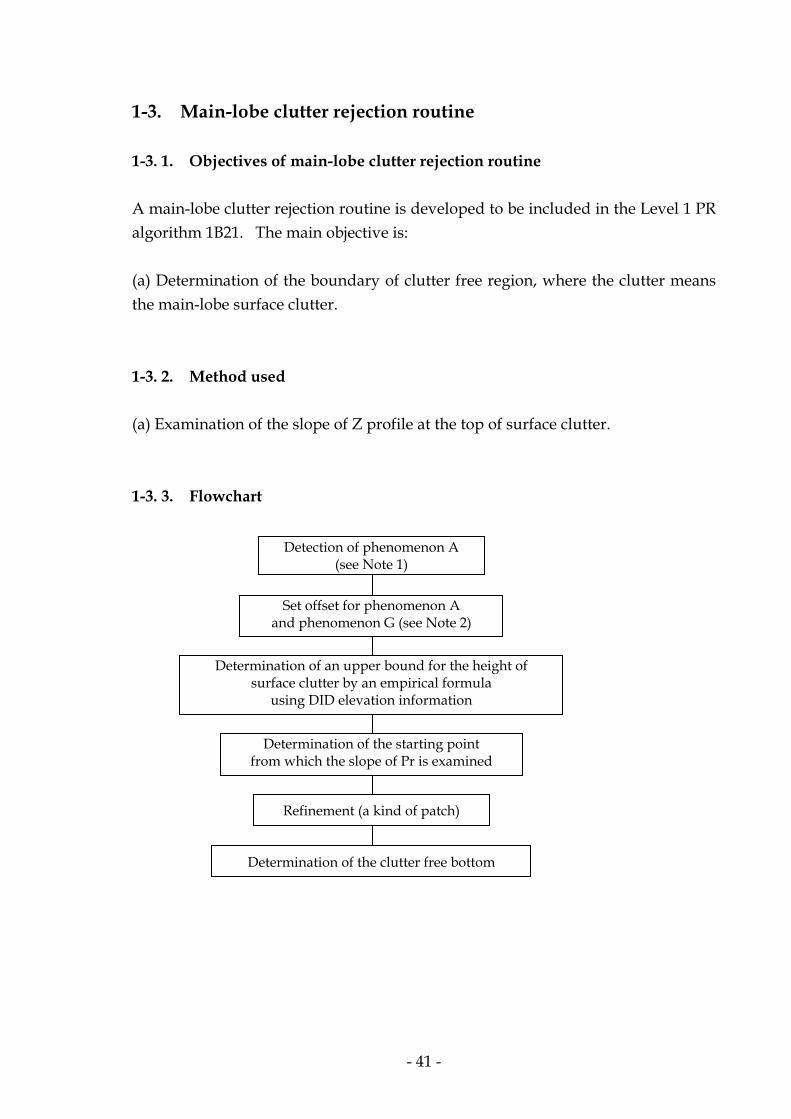
1-3. Main-lobe clutter rejection routine 1-3. 1. Objectives of main-lobe clutter rejection routine A main-lobe clutter rejection routine is developed to be included in the Level 1 PR algorithm 1B21. The main objective is: (a) Determination of the boundary of clutter free region, where the clutter means the main-lobe surface clutter. 1-3. 2. Method used (a) Examination of the slope of Z profile at the top of surface clutter. 1-3. 3. Flowchart
Detection of phenomenon A (see Note 1)
Set offset for phenomenon A and phenomenon G (see Note 2)
Determination of an upper bound for the height of surface clutter by an empirical formula
using DID elevation information
Determination of the starting point from which the slope of Pr is examined
Refinement (a kind of patch)
Determination of the clutter free bottom

- 42 -
Note 1: Description of phenomenon A and phenomenon G. Phenomenon A: Detected position of surface peak is too low from the actual position because of inaccurate DID elevation data, which indicates a too low height. This phenomenon was first observed in the data over the Andes area. Phenomenon G: Detected position of surface peak is too high from the actual position because of inaccurate DID elevation data, which indicates a too high height. This phenomenon was first observed in the data over the Guiana Highlands. Note 2: Detection of phenomenon G is already made before the clutter rejection routine is used in 1B21. 1-3. 4. Outline of the algorithm (a) Detection of phenomenon A: When the radar echo at and around binSurfPeak, which is detected by surface peak detection routine of 1B21, shows that the echo is eventually noise, there may exist the following three possibilities: (1) Phenomenon A occurs because of an inaccuracy of DID elevation data, (2) Strong attenuation makes the radar echo at and around binSurfPeak very small, indistinguishable from noise, (3) The radar echo at and around binSurfPeak is actually very small because of a specular reflection over a very flat surface when the antenna beam points away from the nadir direction. When the radar echo at and around binSurfPeak is very small to be indistinguishable from noise, a search is made upper-wards until an appreciable echo is detected. If the appreciable echo has a peak and has a large slope at the bottom part of the peak, which is typical to the surface clutter, it is judged that the phenomenon A occurs. (b) Offset: Since the clutter rejection code is written in such a way to consult the DID elevation, offset is needed when phenomenon A or G occurs.

- 43 -
(c) Upper bound for the height of surface clutter: Empirical upper bound for the height of surface clutter is obtained by using (i) nominal clutter offset for a flat surface, (ii) maximum height of DID elevation over an 11 km * 11 km box. (d) Starting position of the examination of slope: A point where the received power, Pr, is 10 dB larger than the noise level is used as the starting point from which the slope is examined. If the 10 dB up point is not found, the empirical upper bound obtained by (c) is used as the stating point. (e) Determination of the clutter free bottom: First, whether the stating point obtained by (d) belongs to a rain region or not is examined; if the echo above the starting point has appreciable value and slope is small, it is judged that the starting point belongs to a rain region. If the starting point belongs to a rain region, climb 'up' the surface peak until the slope becomes very large, which is typical to the surface clutter. On the contrary, if the starting point does not belong to a rain region, climb 'down' the surface peak as long as the slope is large. 1-3. 5. Input data
float normalSample_in[49][140], /* unit [dBm]; L1b21swathdata->normalSample */
float osSurf_in[29][5], /* unit [dBm]; L1b21swathdata->osSurf */
float osRain_in[11][28], /* unit [dBm]; L1b21swathdata->osRain */
int osBinStart[29][2], /* L1b21swathdata->osBinStart */
float systemNoise_in[49], /* unit [dBm]; L1b21swathdata->systemNoise */
float zenith[49], /* unit [deg]; L1b21swathdata->scLocalZenith */
float lat[49], /* unit [deg] */
float lon[49], /* unit [deg] */
float scRange[49], /* unit [m]; L1b21swathdata->scRange */
int rayStart[49], /* L1b21header->rayHdr[].rayStart */
int binEllips[49], /* L1b21header->binEllipsoid */

- 44 -
int binSurfP_in[49], /* L1b21swathdata->binSurfPeak */
int Height_mean_in[49], /* unit [m]; mean. of DID elev. (5 km box) */
int Height_max_in[49][2], /* unit [m]; Max. DID elev. [0]: 5 km, [1]: 11 km */
int Height_min_in[49][2], /* unit [m]; Min. DID elev. [0]: 5 km, [1]: 11 km */
int Hmedian_in[49], /* unit [m]; Median of DID elev. 5 km * 5 km */
int Hstd[49], /* unit [m]; RMS dev. 5km * 5km */
int LWflag[49], /* DID land/water/coast flag; 0:W, 1:L, 2:C */
1-3. 6. Output data
int binClutterFreeBottom[49][2], /* bin number with 125 m resol. */
/* (valid range: 1 - 400, and -99) */
int ist[49]. /* status for each bin. */
/* ist[i] = 0: normal, */
/* 1: missing data input and/or */
/* data corruption, */
/* 2: bug (please notify author), */
/* 3: DID elevation doubtful, */
/* 4: binSurfPeak doubtful */
/* maybe due to large ATT, */
/* 5: binSurfPeak doubtful */
/* but not so serious as ist=4. */

- 45 -
1-3. 7. Output file specifications The algorithm 1B21 outputs binClutterFreeBottom[49][2]: ==== In C language ====
int16 binClutterFreeBottom[49][2]:
binClutterFreeBottom[i][0]: range bin number (with 125 m interval) for clutter-free-bottom certain
binClutterFreeBottom[i][1]: range bin number (with 125 m interval) for clutter-free-bottom possible
where i stands for angle bin number running from 0 to 48, and
binClutterFreeBottom[i][0] <= binClutterFreeBottom[i][1]
==== In FORTRAN language ====
INTEGER*2 binClutterFreeBottom (2,49)
binClutterFreeBottom(1,j): range bin number (with 125 m interval) for clutter-free-bottom certain
binClutterFreeBottom(2,j): range bin number (with 125 m interval) for clutter-free-bottom possible
where j stands for angle bin number running from 1 to 49, and
binClutterFreeBottom(1,j) <= binClutterFreeBottom(2,j)

- 46 -
1-3. 8. Interfaces with other algorithms The clutter information, binClutterFreeBottom[49][2], is included in the output of 1B21 and 1C21 HDF files: binClutterFreeBottom[49][2] is used by Level 2 algorithms which need the main-lobe clutter information. 1-3. 9. Special notes (caveats) Since the DID elevation data contains a large error in some area, in particular in high mountain areas, the main-lobe clutter rejection routine has a chance of not being able to output the correct clutter free bottom. Though some improvements are achieved in the product-ver. 6, there still remains the chance of occurring bad clutter free bottom (the occurrence of bad clutter free bottom is estimated to be less than 1 %, but not zero). Tibet and Andes are the most suspicious regions where bad clutter free bottom would still occur. Main changes made in the product-ver. 6 are as follows: (a) Oversample data is used, (b) Added ist=4 and 5 to the output status flag so as to make the re-examination of binSurfPeak more accurately. 1-3.10. References None.
- 47 -
1-4. Redefinition of the Minimum Echo Flag 1-4. 1. Introduction After the TRMM satellite was launched, it was found that sidelobe echoes from the surface at nadir appeared in the radar received signal and that they sometimes were misidentified as rain echoes. In order to decrease the number of such misidentifications, the algorithm for defining the minEchoFlag was modified. A new algorithm was added to redefined the minEchoFlag by using the radar echo signals after removing some of the possible sidelobe echoes. The following section describes the algorithm to remove sidelobe echoes from the original radar echoes for this purpose. Note, however, that the modified radar echoes are used only for this purpose internally, i.e., to redefine the minEchoFlag in 1B21, and that the output data from 1B21 are original radar echoes. Note also that since the parameters for the removal of sidelobe surface echoes are chosen in a conservative way in order not to miss a real rain echo, some of the sidelobe echoes remain to be identified as rain echoes. 1-4. 2. Sidelobe removal algorithm The Precipitation Radar (PR) occasionally observes exceptionally large surface echoes at nadir. Since the PR sensitivity turned out to be better than the minimum requirement, a weak surface echo that is picked up by a sidelobe in the nadir direction appears occasionally in the echo region above the surface when the mainlobe is pointed offnadir. Such sidelobe surface echoes are sometimes identified as rain echoes if they are strong and appear in successive range bins. Since the sidelobe echoes are caused by the reflection of sidelobe signal at nadir, they appear only at the range equal to the nadir range to the surface regardless of the mainbeam direction. Although the magnitudes of the sidelobe echoes naturally correlate with the magnitude of the mainlobe echo at the nadir, the ratio fluctuates substantially from one scan to another. In fact, the sidelobe echoes at different angle bins in a single scan do not correlate very well, either. Therefore, it is not possible to estimate the magnitudes of the sidelobe echoes from the mainlobe nadir return power and to subtract them from the radar echoes at slant incidence angles to remove the sidelobe echoes.

- 48 -
The basic strategy of the sidelobe removing algorithm adopted is as follows:
(1) Find a peak echo around the range corresponding to the nadir surface range,
(2) If this peak value is higher than the signal threshold and if the signals at 500
m above and 500 m below the peak are lower than the threshold, this peak echo and adjacent range bin echoes are identified as sidelobe clutter echoes.
(3) The data identified as sidelobe clutter are replaced by the interpolated data.
However, there are exceptions:
(4) Near the center of swath, the sidelobe range bin is too close to the surface
and the bin 500 m below it is totally contaminated by the mainlobe clutter. In such an angle bin, only the comparison with the data above the expected sidelobe bin is made (in a rather conservative way to avoid missing a true rain echo).
(5) Except around the center of swath, the signal at the same height in the
adjacent (inward) angle bin is also compared with the threshold, and unless this signal is smaller than the threshold, the original peak is not identified as sidelobe echo. This procedure is included to avoid misidentifying the bright band echo as a sidelobe echo.
1-4. 3. Redefinition of minEchoFlag With the data modified in the way explained above, the new algorithm runs the minimum echo detection routine with the rain certain threshold in the same way as the standard routine. If the result is low (not rain certain) and if the original minEchoFlag=20 (rain certain), then the added routine replaces the minEchoFlag of 20 by 13. If the result is high (rain certain) and if the original minEchoFlag=20, then it keeps minEchoFlag as 20 but replaces the binStormHeight for rain certain by the range bin number at which the rain certain flag is first set with the modified data.

- 49 -
Appendix. Detail information of the metadata
ECS (EOSDIS Core System) Metadata Elements [Core Metadata]
Metadata Element
Defined Names of Parameter in the toolkit
0bject Name in the HDF TypeEstimated
size Description
1 Orbit Number TK_ORBIT _NUMBER Orbit Number int 17
The orbit number to be used in calculating the spatial extent of this data.
2 Beginning Date
TK_BEGIN _DATE *****.tkyear *****.tkmonth *****.tkday
Range Beginning Date
date 25
The date when the granule coverage began. Granule coverage defined as the orbit for Level-1 and Level-2 satellite data, as the hour of the granule for Level-1 and Level-2 ground validation data, as the day of the granule for rain gauge and disdrometer data, and as the pentad or month of the granule for Level-3 data.
3 Beginning Time
TK_BEGIN _TIME ***** .tkhour ***** .tkminute ***** .tksecond
Range Beginning Time
time 23 The time when the granule coverage began. See beginning date.
4 Ending Date
TK_END _DATE ***** .tkyear ***** .tkmonth ***** .tkday
Range Ending Date date 22 The date when the granule coverage
ended. See beginning date.
5 Ending Time
TK_END_TIME ***** .tkhour ***** .trminute ***** .tksecond
Range Ending Time time 20 The time when the granule coverage
ended. See beginning date.
6 Granule ID TK_GRANULE _lD
Granule Pointer char 48 ID of granule. Same as input file
name. (ex. 1B12.19990706.1039.1)
7 ID of ECS Data Object TK_DATA_ID Short Name char 66
The unique identifier of an ECS collection to which this granule belongs. (i.e. “Total Power, Noise”, “PR Reflectivity”)
8 Size MB ECS Data Object TK_FILE_SIZE Size MB ECS
Data Granule float 21 The size attribute will indicate the volume of data contained in the granule.
9 Longitude of Maximum Latitude
TK_LON_OF _MAX_LAT
Longitude OfMaximum Latitude
char 50
Longitude of the northernmost extent of the satellite orbit. Decimal degrees with 6 figures precision after the decimal point. Positive east, negative west. A point on the 180th meridian is assigned to the western hemisphere.
10 Spatial Coverage Type
TK_SPAT_COV _TYPE
Spatial Coverage Type char 33
This attribute denotes whether the locality/coverage requires horizontal, vertical or both spatial domain and coordinate system definitions. “both”
11 Ellipsoid Name
TK_ELLIPSOID _NAME Ellipsoid Name char 50 Name of the ellipsoid.
“World Geodetic System (WGS) 84”
12 Equatorial Radius TK_EQ_RADIUS Equatorial
Radius float 51 Equatorial radius of the earth ellipsoid (meters). “6378.137”
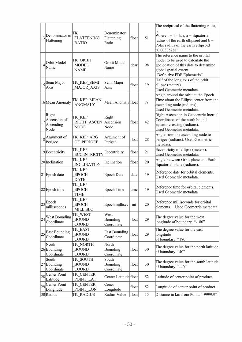
- 50 -
13 Denominator of Flattening
TK _FLATTENING _RATIO
Denominator Flattening Ratio
float 51
The reciprocal of the flattening ratio, f, Where f = 1 – b/a, a = Equatorial radius of the earth ellipsoid and b = Polar radius of the earth ellipsoid “0.00335281”
14 Orbit Model Name
TK_ORBIT _MODEL _NAME
Orbiit Model Name char 98
The reference name to the orbital model to be used to calculate the geolocation of this data to determine global spatial extent. “Definitive FDF Ephemeris”
15 Semi Major Axis
TK_KEP_SEMI _MAJOR_AXIS
Semi Major Axis float 19
Half of the long axis of the orbit ellipse (meters). Used Geometric metadata.
16 Mean Anomaly TK_KEP_MEAN_ANOMALY Mean Anomaly float l8
Angle around the orbit at the Epoch Time about the Ellipse center from the ascending node (radians). Used Geometric metadata.
17
Right Ascension of Ascending Node
TK_KEP _RIGHT_ASCEN_NODE
Right Ascension Node
float 42
Right Ascension in Geocentric Inertial Coordinates of the north bound equator crossing (radians). Used Geometric metadata.
18 Argument of Perigee
TK_KEP_ARG _OF_PERIGEE
Argument of Perigee float 28
Angle from the ascending node to perigee (radians). Used Geometric metadata.
19 Eccentricity TK_KEP _ECCENTRICITY Eccentricity float 21 Eccentricity of ellipse (meters).
Used Geometric metadata.
20 Inclination TK_KEP _INCLINAT10N Inclination float 20 Angle between Orbit plane and Earth
Equatorial plane (radians).
21 Epoch date TK_KEP _EPOCH _DATE
Epoch Date date 19 Reference date for orbital elements. Used Geometric metadata.
22 Epoch time TK_KEP _EPOCH _TIME
Epoch Time time 19 Reference time for orbital elements. Used Geometric metadata
23 Epoch milliseconds
TK_KEP _EPOCH _MILLISEC
Epoch millisec int 20 Reference milliseconds for orbital elements. Used Geometric metadata
24 West Bounding Coordinate
TK_WEST _BOUND _COORD
West Bounding Coordinate
float 29 The degree value for the west longitude of boundary. “-180”
25 East Bounding Coordinate
TK_EAST _BOUND _COORD
East Bounding Coordinate float 29
The degree value for the east longitude of boundary. “180”
26 North Bounding Coordinate
TK_NORTH _BOUND _COORD
North Bounding Coordinate
float 30 The degree value for the north latitude of boundary. “40”
27 South Bounding Coordinate
TK_SOUTH _BOUND _COORD
South Bounding Coordinate
float 30 The degree value for the south latitude of boundary. “-40”
28 Center Point Latitude
TK_CENTER _POINT_LAT Center Latitude float 52 Latitude of center point of product.
29 Center Point Longitude
TK_CENTER _POINT_LON
Cener Longitude float 52 Longitude of center point of product.
30 Radius TK_RADIUS Radius Value float 15 Distance in km from Point. “-9999.9”

- 51 -
3l Latitude Resolution
TK_LATITUDE _RES
Latitude Resolution float 27
The minimum difference between two adjacent latitude values expressed in Geographic Coordinate units of measure. “-9999.9''
32 Longitude Resolution
TK_LONGITUDE_RES
Longitude Resolution float 28
The minimum difference between two adjacent longitude values expressed inGeographic Coordinate units of measure. “-9999.9''
33 Geographic Coordinate Units
TK_GEO _COORD_UNITS
Geographic Coordinate Units
char 112 Units of measure used for the latitude and longitude resolution values. “Decimal Degrees"
34 Temporal Range Type
TK_TEMPOR _RNG_TYPE
Temporal Range Type char 50 This tells the system how temporal
coverage is specified for the granule
35 QA Parameter Name
TK_QA_PARAM_NAME
Qualiity Assurance Parameter Name
char 98 Science Quality Flag
36 QA Parameter Value
TK_QA_P^RAM_VALUE
Quality Assurance Parameter Value
char 99
A post processing indication of quality by the algorithm developer. The Quality Indicator takes the form of 4 possible ASCII strings: ''NOT BEING INVESTIGATED", “BEING INVESTIGATED''. “FAILED" or ”PASSED”.
37 Reprocessing Status
TK_REPRO _STAT
Reprocessing Actual char 40
This attribute identifies the intent of the product author to reprocess the data (i.e. data gaps, geolocation accuracy, scientist review quality flags). “NULL”
38 Browse Package Reference
TK_BROUSE _NAME Browse Pointer char 105
This attribute will contain a system-resolvable reference to an HDF package containing collocation of browse granules. “NULL”
39 Contact Name TK_CONTACT Science Contact char 93
The name of the algorithm developer related to this granule.The contact name supplied here must exist in the ECS contact database. “JAXA Earth Observation Center”.
40 Mean Motion TK_NUN _ORBITS Mean Motion float 50
Number of orbits per day, including fractions of orbits. Used Geometric metadata.
41 Orbit Adjust Flag
TK_ORBIT _ADJUST
Orbit Adjut Flag int 50
Orbit Adjust Flag. Values are as follows: 0 = no orbit adjust activity during this orbit. 1 = orbit adjustment control modes occurred during this orbit.
42 Attitude Mode Flag
TK_ATTITUDE _MODE
Attitude ModeFlag int 50
Attitude Mode flag. Values are as follows: 0 = forward mode (+X forward) throughout this orbit 1 = backward mode (-X forward) throughout this orbit 2 = yaw maneuver during this orbit.
43 Solar beta angle at beginning of granule
TK_BEGIN _SOLAR _BETA
Solar Beta Angle At Beginning Of Granule
float 50 Elevation of sun in the orbit plane at the orbit start (degrees)/ Used Geometric metadata.

- 52 -
44 Solar beta angleat end of granule
TK_END_SOLAR_BETA
Solar Beta Angle At End Of Grnule
float 50 Elevation of sun in the orbit plane at the orbit start (degrees). Used Geometric metadata.
45 Sensor Alignment
TK_SENSOR _ALGN
Sensor Alignment char 100
Euler Sequence (3 integers) and Euler angles for rotation from spacecraft coordinates to sensor coordinates in degrees. (These are to be provided by the science team) “0.0, 0.0, 0.0, 1.2, 3”
46 Sensor Alignment Channel Offsets
TK_SENSOR _ALGN_CHAN _OFFSET
Sensor Alignment Channel Offset
char50*
number of channels
Euler Sequence (3 integers) and Euler angles for rotation from sensor coordinates to Channel coordinate in degrees. (These are to be provided by the science team if needed, but they are not nominally used in TSDIS processing since geolocation is not done per channel) “0”
47 Scan Path Model
TK_SCAN_PATH_MODEL
Scan Path Model char 100
Parameters describing the scan path as used for pixel geolocation. For a (nominal) conical scan model the following parameters are used: Axis of Scan (±1, 2, or 3). Reference Axis for zero rotation angle (±1, 2, or 3), and Scan cone angular radius in degrees. Starting rotation angle relative to the scan axis in degrees. Total rotation angle spanned in degrees, Active scan duration time in seconds (between first and last pixel), and Time Offset between spacecraft time of the sensor data packet and the first pixel time, in seconds. “1.3, 90.0, -17.0, 34.0, 0.3, 0.0”
48 Scan Path Parameters Per Channel
TK_SCAN_PATH_PARAM
Scan Path Model Parameter
char 100
Parameters describing the scan path separately for each channel in degrees. (These are to be provided by the science team if needed, but they are not nominally used in TSDIS processing since geolocation is not done per channel) “0”
49 Ephemeris file descriptor
TK_EPHEM _FILE_NAME
Ephemeris File ID char 50
TSDIS granule ID for the ephemeris file. The format is EPHEM.YYMMDD.nn., where YY is year, MM is month, DD is day of the month, and nn is the version number.
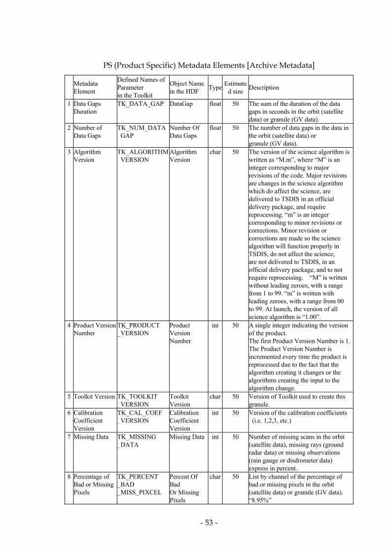
- 53 -
PS (Product Specific) Metadata Elements [Archive Metadata]
Metadata Element
Defined Names of Parameter in the Toolkit
Object Namein the HDF Type Estimate
d size Description
l Data Gaps Duration
TK_DATA_GAP DataGap float 50 The sum of the duration of the data gaps in seconds in the orbit (satellite data) or granule (GV data).
2 Number of Data Gaps
TK_NUM_DATA_GAP
Number Of Data Gaps
float 50 The number of data gaps in the data in the orbit (satellite data) or granule (GV data).
3 Algorithm Version
TK_ALGORITHM_VERSION
Algorithm Version
char 50 The version of the science algorithm is written as “M.m”, where “M” is an integer corresponding to major revisions of the code. Major revisions are changes in the science algorithm which do affect the science, are delivered to TSDIS in an official delivery package, and require reprocessing. “m” is an integer corresponding to minor revisions or corrections. Minor revision or corrections are made so the science algorithm will function properly in TSDIS, do not affect the science, are not delivered to TSDIS, in an official delivery package, and to not require reprocessing. “M” is written without leading zeroes, with a range from 1 to 99. “m” is written with leading zeroes, with a range from 00 to 99. At launch, the version of all science algorithm is “1.00”.
4 Product Version Number
TK_PRODUCT _VERSION
Product Version Number
int 50 A single integer indicating the version of the product. The first Product Version Number is 1. The Product Version Number is incremented every time the product is reprocessed due to the fact that the algorithm creating it changes or the algorithms creating the input to the algorithm change.
5 Toolkit Version TK_TOOLKIT _VERSION
Toolkit Version
char 50 Version of Toolkit used to create this granule.
6 Calibration Coefficient Version
TK_CAL_COEF _VERSION
Calibration Coefficient Version
int 50 Version of the calibration coefficients (i.e. 1,2,3, etc.)
7 Missing Data TK_MISSING _DATA
Missing Data int 50 Number of missing scans in the orbit (satellite data), missing rays (ground radar data) or missing observations (rain gauge or disdrometer data) express in percent.
8 Percentage of Bad or Missing Pixels
TK_PERCENT _BAD _MISS_PIXCEL
Percent Of Bad Or Missing Pixels
char 50 List by channel of the percentage of bad or missing pixels in the orbit (satellite data) or granule (GV data). “8.95%”

- 54 -
9 Maximum Valid Value of Channel
TK_MAX_VALID_CHANNEL
Maximum Valid Value of Channel
char 50 List by channel of the maximum valid value(value specified by the instrument scientist). 1B:”-110”, 1C:”20”
10 Minimum Valid Value of Channel
TK_MIN_VALID_CHANNEL
Minimum Valid Value of Channel
char 50 List by channel of the minimum valid value (value specified by the instrument scientist). 1B:“-20”,1C:“80”
11 Min Max Unit TK_MIN_MAX _UNITS
Min Max Unit char 50 Units of the Minimum and Maximum valid values. 1B: “dBm”, 1C: “dBZ”
12 Orbit Size TK_ORBIT_SIZE OrbitSize int 50 Numbers of scans in Orbit. If the granule is empty, Orbit Size = 0.
13 Radar Wave length
TK_RADAR _WAVELENGTH
Radar Wave length
float 50 Wavelength of the radar (meter). “0.02178”
14 Minimum Reflectivity Threshold
TK_MI_REF _THRESHOLD
Minimum Reflectivity Threshold
float 50 The threshold (dBZ) below which ground based radar reflectivity data is set to the missing value. “-9999.9”
15 Algorithm ID TK_ALGORITHM_ID
Algorithm ID char 50 Name of the algorithm (i.e. 1B21, 1C21)
16 Data Accuracy TK_DATA _ACCURACY
Data Accuracy
char 50 List by channel of the accuracy of the data.
17 Input IDs TK_INPUT _FILES
Input Files char 300 List of input granule IDs. “NULL”
18 Data of Generation of Input Files
TK_GEN_DATE_INPUT_FILES
Data Of Generation OfInput Files
char 50 List of the generation dates of the input files. For ingested files, this is the date TSDIS received the file.
19 Data Center Source Of Input Files
TK_DATA _CENTER_SRC
Data Center Source Of Input Files
char 50 List of the centers generating the input files. e.g., TSDIS NMC.
20 Generation Date
TK_GEN_DATE Generation Date
int 50 Date the dataset was generated.
21 Day/Night TK_DAY_NIGHT Day Night float 50 Percentage scans during the orbit in daytime mode. “-9999.9”
22 Solar Channel Gains
TK_SOLAR _GAIN
Solar ChannelGains
float 50 Channel 1 Mirror Side A Channel 1 Mirror Side B Channel 2 Mirror Side A Channel 2 Mirror Side B
23 SSM/I Adjustment Coefficients
TK_SSMI _ADJUST
SSMI Adjust Coef
float 30 List of the intercepts and slopes defining the following correction to the brightness temperatures for channel: deltaT={A_ch*(tb-250)/50}+B_ch The entries in the list are as follows: 10GHz Vertical adjustment intercept 10GHz Horizontal adjustment intercept19GHz Vertical adjustment intercept 19GHz Horizontal adjustment intercept21GHz Vertical adjustment intercept 37GHz Vertical adjustment intercept 37GHz Horizontal adjustment intercept85GHz Vertical adjustment intercept 85GHz Horizontal adjustment intercept10GHz Vertical adjustment slope 10GHz Horizontal adjustment slope 19GHz Vertical adjustment slope 19GHz Horizontal adjustment slope 21GHz Vertical adjustment slope 37GHz Vertical adjustment slope 37GHz Horizontal adjustment slope 85GHz Vertical adjustment slope

- 55 -
85GHz Horizontal adjustment slope
24 Orbit First Scan UTC Date
TK_FIRST_SCAN_UTC_DATE
Orbit First Scan UTC Date
date 50 Orbit First Scan UTC Date. Date is a 10 character string with the following characters: YYYY/MM/DD, where YYYY = year, MM = month number, DD = day of month and “/” is a literal. If the granule is empty, the value is ‘0/0/0’. In 2A-52, UTC date is stored as “/” is replaced by “-”. In 1B-11 and 2A-12, UTC date is stored in separate words for year, month and day of month.
25 Orbit First Scan UTC Time
TK_FIRST_SCAN_UTC_TIME
Orbit First Scan UTC Time
time 50 Orbit First Scan UTC Time. Time is an 8 character string with the following characters: HH:MM:SS, where HH = hour, MM = minute, SS = second, and “:” is a literal. If the granule is empty, the value is ‘0:0:0’. In 1B-11 and 2A-12, UTC time is stored in separate words for hour, minute, and second.
26 Orbit First Scan UTC Milliscconds
TK_FIRST_SCAN_UTC_MILLISEC
Orbit First Scan UTC Milliseconds
int 50 Orbit First Scan UTC Milliseconds. Milliseconds is a 3 character string with the following characters: MMM, where MMM = the number of milliseconds later than the last whole second.
27 Orbit First Scantime - Spacecraft clock
TK_FIRSTSCAN_SC_SECS
Obit First SCS ecs
int 50 The seconds field of the spacecraft clock time of the first scan in the orbit.
28 Orbit First Scantime - spacecraft Clock Subseconds
TK_FIRSTSCAN_SC_SUBSECS
Orbit First SC Subsecs
int 50 The subseconds field of the spacecraft clock time of the first scan in the orbit.
29 Orbit Last Scan UTC Date
TK_LAST_SCAN_UTC_DATE
Orbit Last Scan UTC Date
date 50 Orbit Last Scan UTC Date. See Orbit First Scan UTC Date.
30 Orbit Last Scan UTC Time
TK_LAST_SCAN_UTC_TIME
Orbit Last Scan UTC Time
time 50 Orbit Last Scan UTC Time. Decided by L1A file header. See Orbit First Scan UTC Time
31 Orbit Last Scan UTC Milliseconds
TK_LAST_SCAN_UTC_MILLISEC
Orbit Last Scan UTC milliseconds
int 50 Orbit Last Scan UTC Milliseconds. See Orbit Last Scan UTC Milliseconds
32 Orbit Last Scantime - Spacecraft clock
TK_LAST_SCAN_SC_SECS
Orbit Last SC Secs
int 50 The seconds field of the spacecraft clock time of the last scan in the orbit.
33 Orbit Last Scantime - Spacecraft clock Subseconds
TK_LAST_SCAN_SC_SUBSECS
Orbit Last SC Subsecs
int 50 The subseconds field of the spacecraft clock time of the last scan in the orbit.
34 UTCF Seconds TK_UTCF_SECONDS
UTCF Seconds
int 50 The second field of the UTCF for the granule.
35 UTCF Subseconds
TK_UTCF _SUBSECONDS
UTCF Subscconds
int 50 The subscconds field of the UTCF for the granule.

- 56 -
36 UTCF Flag TK_UTCF_FLAG UTC Fflag int 50 Flag that indicates the origin of the UTCF. 0 = UTCF was derived from the first ACS packet in the orbit. 1 = a corrected UTFC was used. “0”
37 Leap Second flag
TK_LEAP_SEC _FLAG
Leap Seconds Flag
Int 50 Flag that indicates if a leap second occurred within the granule. 0 = no; 1 = yes.
38 Radar site name
TK_RADAR _NAME
Radars Site Name
char 50 Name of the GV radar or radar site, whichever is applicable. “NULL”
39 Radar city TK_RADAR _CITY
Radar City char 50 Nearest city to the radar site. "NULL”.
40 Radar state TK_RADAR _STATE
Radar State char 50 State or province containing the radar site, if applicable. “NULL”
4l Radar country TK_RADAR _COUNTRY
Radar Country
char 50 Country containing the radar site. "NULL''
42 Number of VOSTK_NUM_VOS Number Of VOS
int 50 The number of volume scans in the granule. “-9999”
43 Radar Grid Origin Latitude
TK_RADAR _ORIGIN_LAT
Radar Grid Origin Latitude
int 50 Latitude (degrees) of the origin. "-9999.9''
44 Radar Grid origin Longitude
TK_RADAR _ORIGIN_LON
Radar Grid Origin Longitude
int 50 Longitude (degrees) of the origin. “-9999.9”
45 Radar Grid Origin Altitude
TK_RADAR _ORIGIN_ALT
Radar Grid Origin Altitude
int 50 Altitude (km) of the origin. “-9999.9”
46 Radar Grid Spacing x
TK_RADAR _SPACING_X
Radar Grid Spacing X
float 50 The zonal interval (km) between grid points. “-9999.9”
47 Radar Grid Spacing y
TK_RADAR _SPACING_Y
Radar Grid Spacing Y
float 50 The meridional interval (km) between grid points. “9999.9”
48 Radar Grid Spacing z
TK_RADAR _SPACING_Z
Radar Grid Spacing Z
float 50 The vertical interval (km) between grid points. “-9999.9”
49 Radar Grid Size x
TK_RADAR _GRID_SIZE_X
Radar Grid Size X
int 50 The number of grid points in the zonal grid direction. “-9999”
50 Radar Grid Size y
TK_RADAR _GRID_SIZE_Y
Radar Grid Size Y
int 50 The number of grid points in the meridional grid direction. "-9999”
5l Radar Grid Size z
TK_RADAR _GRID_SIZE_Z
Radar Grid Size Z
int 50 The number of grid points in the vertical grid direction. “-9999”
52 DZ Cal TK_GV_DZCAL DZ Cal float 50 Radar calibration offset (dBZ). “-9999.9”
53 GVL1C_Scale TK_GV_L1C _SCALE
GV L1C Scale
float 50 Scaling factor for 1C-51 mask (unitless) “-9999.9”
54 Alpha TK_GV_ALPHA Alpha float 50 Correction for gaseous two-way attenuation (dB/km). “-9999.9”
55 Runtime Options
TK_GV _RUNTIME_OPT
Runtime Options
char 100 Runtime options for algorithm including QC parameters used. “NULL”.

- 57 -
56 Anomaly Flag TK_ANOMALY
_FLAG Anomaly Flag char 100 This flag indicates if and why a
granule is empty. The possible values are: “EMPTY: GENERATED AFTER SOFTWARE ERROR” * “EMPTY: NO DATA DUE TO NO RAIN” “EMPTY: NO DATA RECORDED” “EMPTY: DATA RECORDED BUT STILL MISSING” “EMPTY: REASON UNKNOWN” * “NOT EMPTY: POSSIBLE PROBLEM” “NOT EMPTY” * It is expected that satellite data would use only the three values followed by an asterisk. GV data is expected to use all seven values.
57 Software Version
TK_SOFTWARE_VERSION
Software Version
int 50 Version of the Software
58 Database Version
TK_DATABASE_VERSION
Database Version
int 50 Version of PR Database in the PR L1 software
59 Total Quality Code
TK_TOTAL _QUALITV _CODE
Total QualityCode
char 50 Total quality of the PR L1 product. Range is ‘G’, ‘F’, or ‘P’.
60 Longitude on the Equator
TK_LON_ON _EQUATOR
Longitude On Equator
float 50 Longitude on the equator from the ascending node. Range is -180.000 to 179.999.
61 UTC Date on the Equator
TK_UTC_DATE _ON_EQUATOR
UTC Date On Equator
date 50 UTC date on the equator. See Orbit First Scan UTC Date.
62 UTC Time on the Equator
TK_UTC_TIME _ON_EQUATOR
UTC Time On Equator
time 50 UTC time on the equator. See Orbit First Scan UTC Time.
63 UTC milliseconds on the Equator
TK_UTC _MILLSEC_ON _EOUATOR
UTC Millisecs On Equator
int 50 UTC millisecond on the equator. See Orbit First Scan UTC Milliseconds.
64 Orbit center scan UTC date
TK_CENTER _SCAN _UTC_DATE
Center Scan UTC Date
date 50 UTC date at orbit center scan. See Orbit First Scan UTC Date.
65 Orbit center scan UTC time
TK_CENTER _SCAN _UTC_TIME
Center Scan UTC Time
time 50 UTC time at orbit center scan. See Orbit First Scan UTC Time.
66 Orbit Center scan UTC milliseconds
TK_CENTER _SCAN _UTC_MILLISEC
Center Scan UTC Millisec.
int 50 UTC milliseconds at orbit center scan. See Orbit First Scan UTC Milliseconds.
67 Orbit first scan latitude
TK_FIRST_SCAN_LAT
FirstScanLat float 50 Latitude of orbit first scan. Range is -40.000 to 40.000
68 Orbit first scan longitude
TK_FIRST_SCAN_LON
First Scan Lon
float 50 Latitude of orbit first scan. Range is -180.000 to 179.999.
69 Orbit last Scan latitude
TK_LAST_SCAN_LAT
Last Scan Lat float 50 Latitude of orbit last scan. Range is -40.000 to 40.000.
70 Orbit last scan longitude
TK_LAST_SCAN_LON
Last Scan Lon float 50 Longitude of orbit last scan. Range is -180.000 to 179.999.
71 Number of Rain Scans
TK_NUM_0F _RAIN_SCAN
Number Of Rain Scans
int 50 Number of rain scan whose Minimum Echo Flag is 1 or 2.
- 58 -
2. Level 2 2-1. 2A-21: Surface Cross Section 1. Objectives and functions of the algorithm
The primary objective is to compute the path-integrated attenuation (PIA) using the surface reference technique (SRT). The surface reference technique rests on the assumption that the difference between the measurements of the normalized surface cross section within and outside the rain provides a measure of the PIA. An estimate of the rain-free normalized radar surface cross section (σ0 or NRCS) is used as a reference value for computing the PIA. The algorithm selects the “best” of four types of reference estimates that may be computed. The estimates used are
Along-track Spatial Average. An average of the Ns most recent rain-free σ0 measurements in same angle bin and with the same surface type (currently Ns=8).
In the text below, this estimate is referred to as the spatial average.
Temporal Average. An average at each angle bin of the σ0 data at 1°×1° latitude-longitude cell computed over the month.
Global Average. A global mean σ0 classified by surface type and angle bin,
computed for a “typical” month.
Cross-track Hybrid. A reference data set that results from a quadratic fit of the along-track spatial average data over the 49 angles bins within the cross-track swath. This is explained below in more detail.
In addition to the sample mean of the NRCS as a function of angle bin (and in some cases location or surface type), the reference data sets also include the standard deviation of each of the sample means. This quantity is used to estimate the stability of the reference rain-free mean NRCS. In the spatial surface reference data set, the mean and standard deviation of the NRCS are calculated over a running window of Ns fields of view before rain is encountered (currently, Ns=8). These operations are performed separately for each of the 49+2 incidence angles of TRMM, corresponding to the cross-track scan from -17° to +17° with respect to nadir. The 2 additional angle bins (making the total 51 rather than 49) are used to take care of non-zero pitch/roll angles that can shift the incidence angle outside the normal range. For the temporal surface reference data set, the running mean and standard deviation are computed over a 1°×1° (latitude, longitude) grid. Within each 1°×1° cell, the data are further categorized into incidence angle categories (26). The number of observations in each category, Nt, is also recorded.

- 59 -
Note that in the temporal reference data set no distinction is made between the port and starboard incidence angles so that instead of 49 incidence angles, there are only 25+1, where the additional bin is used to store data from angles outside the normal range. As of version 6, a new method of estimating surface reference values is used for ocean scans. This hybrid method takes the spatial surface reference data set for the entire scan and computes a cross-track fit. The assumption is that the cross-track angular dependence of the surface cross section can be approximated by a quadratic. As implemented, this method applies only to scans that are entirely over ocean. Whenever this condition is met, and hybrid estimate can be computed, then it will be chosen in preference to the spatial and temporal estimate. See section 8 for more detail about the hybrid method. When rain is encountered, the mean and standard deviations of the reference σ0 values are retrieved from the spatial and temporal surface reference data sets. To determine which reference measurement is to be used, the algorithm checks whether Nt ≥ Ntmin and Ns ≥ Nsmin, where Ntmin and Nsmin are the minimum number of samples that are needed to be considered a valid reference estimate for the temporal and spatial reference data sets, respectively. (Currently, Ntmin=50 and Nsmin=8.) If neither condition is satisfied, no estimate of the PIA is made and the flags are set accordingly (see below). If only one condition is met, then the surface reference data that corresponds to this is used. If both conditions are satisfied, the surface reference data is taken from that set which has a smaller sample standard deviation. If a valid surface reference data set exists (i.e., either Nt ≥ Ntmin or Ns≥Nsmin or both) then the 2-way path attenuation (PIA) is estimated from the equation: PIA = σ 0(reference value) −σ 0(in rain) where σ0(in rain) is the value of the normalized radar surface cross section over the rain volume of interest and <σ0(reference_value)> is the mean value obtained from either the temporal or spatial reference data sets, the choice of which depends on the considerations discussed above. The hybrid estimate is computed after the entire scan has been processed as described above. If the hybrid estimate is computable (entire scan is over ocean, and spatial estimates exist for a sufficient number of angle bins, Nh≥Nhmin [currently, Nhmin =5]), then the hybrid estimate is substituted for the previously selected estimate. To obtain information as to the reliability of this PIA estimate we consider the ratio of the PIA, as derived in the above equation, to the standard deviation as calculated from the rain-free σ0 values and stored in the reference data set. Labeling this as std_dev(reference value), then the reliability factor of the PIA estimate is defined as:
reliabFactor =PIA
std_dev(reference value)

- 60 -
When this quantity is large, the reliability is considered high and conversely. This is the basic idea. Specific definitions of the reliability flag and reliability factors are given in the definitions of the output variables. Description of the HDF output variables for 2a-21 can be found in Volume 4 - levels 2 and 3 file specifications available at: <http://tsdis02.nascom.nasa.gov/tsdis/Documents/ICSVol4.pdf> Two comments should be made. i. The PIA is often defined as the one-way path attenuation rather than the 2-way
attenuation used here. Note also that the PIA(2-way) is related to the specific attenuation or attenuation coefficient k (dB/km) by the equation: PIA(2 - way) = 2 k(s) ds
0
rs∫
where the path integral is taken along the direction of the main beam and where the integration limits range from the radar to the surface. Since the attenuation from the radar to the storm top is negligible, the integral can also be thought of as going from the storm top to the surface.
ii. A case can be made for defining the reliability factor other than that given above. For
example, we can define reliability factors by:
Rel = PIA - std_dev(reference value)PIA
Re ′ l = PIA - std_dev(reference value) so that Rel=1 (or Rel’ = PIA) would correspond to a perfect estimate whereas increasingly smaller values of Rel (including negative values) would correspond to lower reliabilities. Since the numerator and denominator of the expressions for Rel and Rel’ can be computed from the output data, these quantities can be easily generated.

- 61 -
2. Command line arguments: 1B21.inputfile.HDF the 1B-21 HDF file 2A21.outputfile.HDF the 2A-21 HDF output file 2A21.int_tr.dat the read-only temporal intermediate file 2A21.int_tw.dat the write-only temporal intermediate file 2A21.int_s.dat the spatial intermediate file 2A21.diag the verification (diagnostic) file
Note that the verification file is created in the program and should not exist prior to execution.
3. Definitions of Output Variables
sigmaZero(49) [real*4] Normalized backscattering radar cross section of the surface (dB) (NRCS) for the 49 angles bins in the radar scan (unitless). rainFlag(49) [integer*2] Rain/no-rain flag (rain=1; no-rain=0) The rain possible category from 1B-21 is included in the no-rain category; only the rain-certain category is considered rain. incAngle(49) [real*4] Incidence angle with respect to nadir (in degrees); pitch/roll correction is included. pathAtten(49) [real*4] Estimated 2-way path-attenuation in (dB) where
pathAtten = 2 k(s)ds0
rs
∫
where k(s) is the attenuation coefficient in dB/km and integral runs from storm top to the surface. The path attenuation is often designated as the PIA, the path-integrated attenuation. reliabFlag(49) [integer*2] Reliability Flag for the PIA estimate, pathAtten, defined below. reliabFactor(49) [real*4] Reliability Factor for the PIA estimate, pathAtten, defined below.

- 62 -
3.1 Definition of reliabFlag reliabFlag = 10000*iv + 1000*iw + 100*ix + 10*iy + iz where iv is a rain/no-rain indicator iw is an indicator of the reliability of the PIA estimate ix indicates the type of surface reference used iy provides information about surface detection iz gives the background type iv = 1 (no rain along path) = 2 (rain along path) iw = 1 (PIA estimate is reliable) - see definitions below = 2 ( is marginally reliable) = 3 ( is unreliable) = 4 ( provides a lower bound to the path-attenuation) = 9 (no-rain case) ix = 1 (spatial surface reference is used to estimate PIA) = 2 (temporal “ “ “ PIA) = 3 (neither exists — i.e. insufficient number of data points) = 4 (unknown background type) = 5 (no-rain case & low SNR — do not update temporal or spatial SRs) = 6 (global surface reference) = 7 (cross-track-spatial hybrid surface reference) = 9 (no-rain case) iy = 1 (surface tracker locked - central angle bin) = 2 ( unlocked - central angle bin) = 3 (peak surface return at normally-sampled gate - outside central swath) = 4 ( not at normally-sampled gate - outside central swath) iz = 0 (ocean) = 1 (land) = 2 (coast) = 3 (unknown or of a category other than those above or ‘mixed’ type) Note: for missing data set reliabFlag = -9999

- 63 -
3.2 Definition of reliabFactor reliabFactor = pathAtten/std_dev(reference value) where PIA is the 2-way path-integrated attenuation (dB), and std_dev(reference value) is the standard deviation as calculated from the no-rain σ0 values. Both quantities are in dB. In versions 1-4 of the algorithm, the reliabFactor was defined as the difference: pathAtten - std_dev(reference value) rather than the ratio pathAtten/std_dev(reference value) The parameter iw (in reliabFlag) is determined from reliabFactor and the SNR of the surface return (in dB). As currently defined: iw = 1 (reliable) if ((reliabFactor ≥ 3) and (SNR(dB) > 3)) = 2 (marginally reliable) if ((reliabFactor ≥ 1) and (reliabFactor < 3) and (SNR(dB) > 3)) = 3 (unreliable) if either (reliabFactor < 1) or ((SNR(dB) ≤ 3).and.(reliabFactor < 3)) = 4 (lower bound) if ((reliabFactor ≥ 3) and (SNR(dB) ≤ 3)) [The iw = 4 case is defined because, while the attenuation estimate will be negatively biased because of a low signal-to-noise ratio, it may lead to the best rain estimate possible under the circumstances.] [SNR is the signal-to-noise ratio; expressed in dB this is given by the difference between the noise-corrected radar return power (dBm) and the radar noise power (dBm)] Note: for missing data, set reliabFactor = -9999.9 Note: pathAtten can assume both positive and negative values. Negative values have a negative reliabFactor, they are marked unreliable (iw=3). Before version 6, negative pathAtten were set to zero.

- 64 -
4. Description of the Processing Procedure:
At each angle bin, calculate the normalized radar surface cross section, σ0, and check whether rain is present. Also, find the (1°×1° × angle-bin) element into which the measurement falls. If rain is present, retrieve the mean and standard deviations from the temporal and spatial reference data sets (formed from previously measured data under rain-free conditions). If both temporal and spatial reference data sets satisfy certain conditions, check which sample mean has the lower variance. Using the sample mean associated with the smaller variance, compute an estimate of the path-integrated attenuation and an associated reliability factor. If neither the spatial nor temporal reference data satisfy these conditions, use the global reference. In version 6, check the following conditions: the entire scan is over ocean and the spatial reference exists in at least Nhmin (Nhmin =5) angles bins (out of a total of 49) within the scan; if these two conditions hold, then the hybrid reference data is used (section 8). If rain is absent, update the temporal statistics (mean and mean-square) of σ0 at the relevant (1°×1° × angle-bin) element. Also, update the spatial statistics of σ0. 5. Interfaces to other algorithms:
All input data for this algorithm is from 1B-21; the outputs are used by 2A-25, 3A-25 and 3A-26. 6. Comments and Issues:
a. A gaussian beam approximation is used to represent the TRMM antenna pattern. b. The radar return power used in computing σ0 is that for which a 2.5 dB correction has
been made. The factor accounts for the logarithmic averaging loss. Like the rain, the surface is treated as a Rayleigh target.
c. σ0 is being computed from that (single) gate where the return power is a (local)
maximum. d. The algorithm assumes that rain is present only if minEchoFlag = 2 (rain certain);
minEchoFlag = 1 (rain possible) and minEchoFlag = 0 (rain absent) are treated as no-rain cases. Note that the minEchoFlag variable is read from 1B-21.

- 65 -
e. Before version 6, images of path attenuation from 2A-21 sometimes showed a striated
or streaky pattern where the attenuation estimates at one or more angles are larger than the estimates at adjacent angles. This occurred more often at near-nadir angles where high values of the surface cross section are observed under rain-free conditions. Where it is used, the cross-track-spatial hybrid method appears to eliminate most of these streaky patterns.
f. The diagnostic file includes attenuation and reliability results from several alternative
methods:“standard” [version 5], cross-track, and hybrid, with 3 alternative reliabFactor formulas. Each entry is written on one line with the following fields: method - A text string identifying the method scan number angle bin number PIA reliabFactor reliabFlag The method ID values are: stdPIA Version-5 standard PIA (spatial or temporal) xTrack Cross-track method (ocean only) xtHyb1 Hybrid method, reliabFactor=A/chisqr xtHyb2 Hybrid method, reliabFactor=A/avg(sd) xtHyb3 Hybrid method, reliabFactor=A/rms(sd) In the reliabFactor formulas above, A is the Hybrid PIA, chisqr is the reduced Chi-square for the cross-track fit, sd is the standard deviation for the individual spatial average for the current angle bin, and rms(sd) is the root-mean-square of the sd’s over all angle bins for the current scan. The value written in the HDF file is xtHyb3. The “xTrack” method is another experimental cross-track method that uses non-rain angle bins in the current scan. It is computed only if the scan includes a mixture of rain and non-rain angle bins, all over ocean. This method was experimentally introduced in version 5. Because each line is labeled with the method ID, the diagnostic file can easily be divided into separate files for each method. Examples of this are shown in the following Unix commands: egrep 'stdPIA' 2A21.990913.10321.6.diag | cut -d: -f2 > stdpia egrep 'xTrack' 2A21.990913.10321.6.diag | cut -d: -f2 > xtrack egrep 'xtHyb1' 2A21.990913.10321.6.diag | cut -d: -f2 > xthy1 egrep 'xtHyb2' 2A21.990913.10321.6.diag | cut -d: -f2 > xthy2 egrep 'xtHyb3' 2A21.990913.10321.6.diag | cut -d: -f2 > xthy3

- 66 -
g. In previous versions of the algorithm (versions 1-4) the reliabFactor was defined
as the difference: pathAtten - std_dev(reference value). In version 5 and 6, reliabFactor is defined as the ratio: pathAtten/std_dev(reference value).
h. Prior to version 6, when the PIA < 0, pathAtten was set to 0.0. reliabFactor,
which in version 5 is proportional to PIA, was computed before pathAtten was set to 0, so it could be negative; pathAtten was never less than zero. In version 6, pathAtten is no longer set to zero. Negative values are possible, although they will always be marked unreliable in the reliabFlag.
7. Description of Temporal Intermediate File
Two temporal intermediate files are used to store (write-only file) and read (read-only file) the rain-free statistics of the normalized surface cross sections as a function of incidence angle (26 categories) and location (1°×1° latitude-longitude grid). For the first month of data (December, 1997), the read-only and write-only temporal intermediate files are initialized to zero. During the processing of data from this month, the rain-free statistics are continuously updated and stored in the write-only file. At the end of the month, the write-only file for December is used as the read-only file for January and the write-only file is re-initialized to zero. This means that for the data processed in January, the statistics compiled in December will be used for the temporal reference data set. At the end of the processing of the January data, the write-only file, used to store the statistics for January, is used as the read-only file for the month of February. In general, the write-only file from the previous month is used as the read-only file (i.e. the reference data set) for the present month and where the write-only file is re-initialized at the beginning of each month. At the beginning of the post-boost data processing, the temporal files are set to zero. In particular, for the first segment of post-boost data (Aug. 2001), the read-only intermediate files are zeroed out. For the next month, the read-only files are converted to the write-only file and used as the temporal reference data for Sept. 2001.

- 67 -
8. The Cross-track Hybrid Surface Reference Method
2A-21 v5 computes the Path Integrated Attenuation (PIA) for each angle bin using spatial and temporal averages, selecting the method that gives the largest reliability factor. Version 6 also implements two alternative “cross-track” methods for ocean scans. The results of these methods are written in the diagnostic file along with the v5 result. When appropriate, the “cross-track hybrid” PIA is chosen as the 2A-21 product. Both methods perform a cross-track quadratic fit of the reference surface cross sections. The xtrack method fits a quadratic using data from all rain-free angle bins in the current scan; the hybrid method fits a quadratic using data from the current along-track spatial average at each angle bin. If the rain region is extensive, the xtrack method may have few or no data points to fit; if enough data are available to fit, the points will always be near the rain observations because they are taken from the same scan. The hybrid method always (or almost always) has a full scan worth of data to fit. The 49 spatially-averaged data points have the same potential problems as the standard spatial average, namely, that in some cases the spatial average might be computed in a region remote from the current IFOV, so that the rain-free along-track spatial averages are computed over ocean areas that are far from the rain cell in questions. (By examining the reference data for an orbit of data processed in reverse order we find that the spatial averaged reference data can differ significantly particularly in coastal regions.) The spatial average for each angle bin is computed over the last 8 rain-free observations over the same background type (i.e., ocean, land, or coast). The standard deviation from the spatial average is used as a weight in the fitting procedure. The fitted function is a quadratic where the fitting routine is based on the LFIT routine from Numerical Recipes (Press, et. al., 1989). The spatial average at the ith angle bin is the average of the last 8 rain-free surface reflectivity values, σ0
NR, yi = σ NR
0 (θi) and, using “AS” to denote the along-track spatial reference, the standard deviation is SAS(θi) = var(σ NR
0 (θi)) The fit function is the quadratic yfit(θi) = a + bθi + cθi
2

- 68 -
We determine the parameters a, b, and c by minimizing
χ 2 =yi − yfit(θi)
SAS(θi)
2
i=1
49
∑
The (2-way) hybrid PIA is the difference between the Surface Reference value, yfit(θi), and the apparent (attenuated) surface cross section, σ0
i: Ai = yfit(θi) −σ i
0 At this point, it is unclear what reliability factor is appropriate for the cross-track hybrid PIA estimate. Currently, the program computes three candidate values and writes them to the diagnostic file. The reliability factor is a ratio of the PIA estimate to an estimate of the uncertainty. The difference between the candidate factors is the choice of uncertainty estimate. For the standard spatial average product, the uncertainty estimate is the standard deviation of the spatial average. (For the temporal average it is the standard deviation of the temporal average. The question of whether these choices are the most appropriate, and whether or not they represent the best criteria for selecting between spatial and temporal estimates is unresolved.) Three alternative reliability factors are described below; the third, based on the RMS of the spatial averages across the scan, is used in the HDF in version 6. The first hybrid reliability factor is based on the reduced chi-square for the fit,
χN−32 =
χ 2
N − 3
N is the number of angle bins, usually N=49. The reliability factor is
reliabFactor_1(i) =Ai
χN−32
Two alternate reliability factors are based on the sum of the standard deviations from with the along-track spatial reference, SAS, and on the RMS of SAS:
reliabFactor_2(i) =Ai
149
SAS(θ j )j=1
49
∑
and
reliabFactor_3(i) =Ai
rms(SAS)

- 69 -
Where
rms(SAS) =149
SAS2 (θ j )
j=1
49
∑
In version 6, reliabFactor_3 is the value included in the HDF product. 9. Revised Angle Bin Definitions
2A-21 defines two angle bins. The first, angle1, is computed from the absolute value of the incidence angle, and is used to categorize observations for the temporal Surface Reference Technique (SRT). It ranges from 1 to 26 (Fortran array convention). The other angle bin, angle2, depends on the signed incidence angle, and is used for the spatial SRT. It ranges from 1 to 51. The angle bins angle1 and angle2 are defined such that angle1−1− 0.5( )∆θ ≤ θ < angle1−1+ 0.5( )∆θ angle2 − 26 − 0.5( )∆θ ≤ θ < angle2 −1+ 0.5( )∆θ where θ is the incidence angle and ∆θ is the angle bin size. These relations can be expressed more simply by
angle1= intθ
∆θ+1+ 0.5
angle2 = int θ∆θ
+ 26 + 0.5
respectively. There was a problem with the implementation of this algorithm before version 6: ∆θ was defined as the cross-track beam width, which is read from the 1B-21 Ray Header. The beam positions (as opposed to the beam width) are uniformly spaced with equal steps of 0.75°. One effect of the old angle bin definition is that the angle bins were not uniformly populated. In general, each scan should have one beam position in each “angle2 bin” except for the extra edge bins (1 and 51). In fact, some bins were under-populated and some were over-populated because the angle bins did not correspond with the actual beam spacing. In version 6 of the 2A-21 algorithm, ∆θ has been set to a constant value of 0.75°.

- 70 -
10. References
Caylor I.J., G.M. Heymsfield, R. Meneghini, and L.S. Miller, 1997: Correction of sampling errors in ocean surface cross-sectional estimates from nadir-looking weather radar. J. Atmos. Oceanic Technol., 14, 203-210. Iguchi, T. and R. Meneghini, 1994: Intercomparisons of single-frequency methods for retrieving a vertical rain profile from airborne or spaceborne radar data. J. Atmos. Oceanic Technol., 11, 1507-1516. Kozu, T., 1995: A generalized surface echo radar equation for down-looking pencil beam radar. IEICE Trans. Commun., E78-B, 1245-1248. Marzoug, M. and P. Amayenc, 1994: A class of single- and dual-frequency algorithms for rain rate profiling from a spaceborne radar. Part I: Principle and tests from numerical simulations. J. Atmos. Oceanic Technol., 11, 1480-1506. Meneghini, R., T. Iguchi, T. Kozu, L. Liao, K. Okamoto, J.A. Jones, and J. Kwiatkowski, 2000: Use of the surface reference technique for path attenuation estimates from the TRMM Radar. J. Appl. Meteor., 39, 2053-2070. Meneghini, R. and K. Nakamura, 1990: Range profiling of the rain rate by an airborne weather radar. Remote Sens. Environ., 31, 193-209. Meneghini, R., J.A. Jones, T. Iguchi, K. Okamoto, and J. Kwiatkowski, 2004: A hybrid surface reference technique and its application to the TRMM Precipitation Radar, J. Atmos. Oceanic Technol., 21, 1645-1658.
- 71 -
2-2. 2A23 2-2.1. Objectives of 2A23 Main objectives of 2A23 are as follows:
(a) Detection of bright band (BB) and determination of the height of BB, the strength of BB, and the width (i.e. thickness) of BB when BB exists.
(b) Classification of rain type into the following three categories:
- stratiform, - convective, - other, where "other" means (ice) cloud only and/or maybe noise. (c) Detection of shallow isolated and shallow non-isolated. (d) Output of Rain/No-rain flag. (e) Computation of the estimated height of freezing level. (f) Output of the height of storm top. 2-2.2. Main changes from the previous version The current product version of 2A23 is V6 (version 6). Main changes are as follows:
(a) Rain type is expressed by 3-digits number, while in the previous versions by 2-digits number.
(b) Shallow non-isolated (type of rain) is newly detected in addition to the
V5-existing shallow isolated. (c) All the shallow isolated are classified as convective in V6, while in V5 most
of the shallow isolated are stratiform. In contrast to shallow isolated, the rain type of non-shallow isolated can be stratiform/convective/other depending on its intensity.

- 72 -
(d) Changed the criteria for other type, which makes a substantial decrease in
the number of other type of rain. (e) When rain is 'certain' and rain type is 'other', it most probably indicates that
there exists ice cloud only. (f) When BB is detected, rain type is stratiform. (In the previous versions,
however, rain type can be convective even though BB is detected in a very exceptional case.)
(g) Oversample data are used in the detection of BB, and oversample range bin
numbers are used for computing heights. (h) Upper and lower boundaries of BB, and the width of BB are added to the
output. (i) Improvement in BB detection is made. (j) Changed a convective threshold in H-method from 40 dBZ to 39 dBZ; the
effect of this change, however, is very small. (k) Rain probable is introduced. (Internal use in 2A23 only, and the type of
rain probable is other.)
2-2.3. Method used in 2A23 (a) Detection of bright band (BB): - Peak search by (1) using a spatial filter method [1], and (2) examining the slope in the upper part of BB profile. In the peak search, several conditions are imposed on the height profile of BB.
(b) Determination of the width of BB: - By detecting upper and lower boundaries of BB along the slant path, then computing the thickness (i.e. width) of BB.
(c) Rain type classification: - Vertical profile method (V-method)[1], - Horizontal pattern method (H-method)[2].
- 73 -
(d) Detection of shallow isolated and shallow non-isolated: - A simple examination of the height of storm top being much lower than the estimated height of freezing level. When an isolation condition is satisfied, the type is shallow isolated, otherwise shallow non-isolated. Here, the isolated condition means that the shallow area is isolated from the non- shallow area.
(e) Rain/No-rain flag: - Almost identical to minEchoFlag recorded in 1C21 HDF file. Difference occurs when rain probable is detected or, on rare occasion, when corrupted input data are detected.
(f) Estimated height of freezing level: - Temporal and spatial interpolation of a climatological surface temperature at the sea level, and a use of a constant lapse rate of temperature.
(g) Height of storm top: - A simple conversion from range bin number to the height above the sea level.
2-2.4. Processing Flow
(1) Open files.
(2) Read in 1C21 metadata, and copy the metadata to 2A23 HDF file.
(3) Read in a static data for the estimation of the height of freezing level (freezH).
(4) Read in scan header from 1C21 HDF file.
(5) Repeat reading in 1C21 scan data until the end of 1C21 HDF file, and do the following data processing for each scan: (a) Estimate freezH. (b) Compute the height of storm top (stormH). (c) Detect sidelobe clutter. (d) Detect BB. When BB is detected, compute the height of BB, the strength of
BB, upper and lower boundaries of BB, and the width of BB, and set the status flag on BB detection.
(e) Classify rain type by V-method. Reject sidelobe clutter during this processing.
(f) Detect shallow isolated and shallow non-isolated.

- 74 -
(g) Classify rain type by H-method. Reject sidelobe clutter during this processing.
(h) Unify rain types. (i) Set status flag. (j) Write output to 2A23 HDF file.
(6) Close files and end the processing. 2-2.5. Input data (a) From 1C21 HDF file:
(1) metadata (2) rayHdr[49].rayStart (scan header) (3) rayHdr[49].startBinDist (scan header) (4) scanStatus.missing (L1C_21_SWATHDATA) (5) scanStatus.dataQuality (L1C_21_SWATHDATA) (6) geolocation[49][2] (L1C_21_SWATHDATA) (7) minEchoFlag[49] (L1C_21_SWATHDATA) (8) binStormHeight[49][2] (L1C_21_SWATHDATA) (9) binEllipsoid[49] (L1C_21_SWATHDATA) (10) binClutterFreeBottom[49][2] (L1C_21_SWATHDATA) (11) binDIDHmean[49] (L1C_21_SWATHDATA) (12) scLocalZenith[49] (L1C_21_SWATHDATA) (13) scRange[49] (L1C_21_SWATHDATA) (14) osBinStart[29][2] (L1C_21_SWATHDATA) (15) landOceanFlag[49] (L1C_21_SWATHDATA) (16) binSurfPeak[49] (L1C_21_SWATHDATA) (17) normalSample[49][140] (L1C_21_SWATHDATA) (18) normalSample_scale[49][140] (L1C_21_SWATHDATA) (19) osSurf[29][5] (L1C_21_SWATHDATA) (20) osRain[11][28] (L1C_21_SWATHDATA)
(b) From sst-hou.grd file (for the estimation of freezH):
(1) sstdata[144][91][2]

- 75 -
2-2.6. Output data (1) metadata (2) scanTime ---- same as that of 1C21 (3) geolocation[49][2] ---- same as that of 1C21 (geolocation(2,49) in FORTRAN) (4) scanStatus (structure) ---- same as that of 1C21 (5) navigate (structure) ---- same as that of 1C21 (6) rainFlag[49] Rain/No-rain flag (1-byte integer) (7) rainType[49] Rain type (2-byte integer) (8) shallowRain[49] Shallow rain flag (1-byte integer) (9) status[49] Status (1-byte integer) (10) binBBpeak[49] Range bin number for BB (2-byte integer) (11) HBB[49] Height of BB [m] (2-byte integer) (12) BBintensity[49] Strength of BB [dBZ] (4-byte float) (13) freezH[49] Estimated height of freezing level [m] (2-byte integer) (14) stormH[49] Height of storm top [m] (2-byte integer) (15) BBboundary[49][2] Upper and lower boundaries of BB (2-byte integer) (BBboundary(2,49) in FORTRAN) (16) BBwidth[49] Width of BB [m] (2-byte integer) (17) BBstatus[49] Status flag for BB (1-byte integer) (18) spare[49] Spare (2-byte integer) 2-2.7. Output file specifications This section describes details of items (6)-(17) in the previous section. (a) int8 rainFlag[49]: = 0 : no rain 10 : rain possible 11 : rain possible 12 : rain possible 13 : rain possible 15 : rain probable 20 : rain certain -99 : data missing
- 76 -
Note: rainFlag is almost identical to minEchoFlag of 1C21 except for rain probable case and the following very exceptional case. The exception occurs if 2A23 detects data missing but 1C21 says the data is normal - this can happen when the input data is corrupted. In normal conditions, the rain certain case in rainFlag is identical to the rain certain case in minEchoFlag of 1C21. (b) int16 rainType[49]: In V6 of 2A23, the flag rainType[i] (i=0 to 48) indicates the unified rain type by 3-digits numbers. (Beware that, in V5 and earlier, rain type is expressed by 2-digits numbers. Also note that the variable type of rainType is changed from int8 in V5 to int16 in V6.) rainType[i] = 100: Stratiform. When R_type_V[i] = T_stra, (BB detected) and R_type_H[i] = T_stra; 110: Stratiform. When R_type_V[i] = T_stra, (BB detected) and R_type_H[i] = T_other; 120: Probably stratiform. (BB may exist but not detected) When R_type_V[i] = T_other, and R_type_H[i] = T_stra; 130: Maybe stratiform. When R_type_V[i] = T_stra, (BB detected) and R_type_H[i] = T_conv; 140: Maybe stratiform. (BB hardly expected) When R_type_V[i] = T_other, and R_type_H[i] = T_stra; 152: Maybe stratiform: When R_type_V[i] = T_other, R_type_H[i] = T_stra, and shallowRain[i] = 20 or 21; (Shallow non-isolated is detected)

- 77 -
160: Maybe stratiform, but rain hardly expected near surface. BB may exist but is not detected. When R_type_V[i] = T_other; and R_type_H[i] = T_stra; 170: Maybe stratiform, but rain hardly expected near surface. BB hardly expected. Maybe cloud only. Distinction between 170 and 300 is very small. When R_type_V[i] = T_other; and R_type_H[i] = T_stra; 200: Convective When R_type_V[i] = T_conv, and R_type_H[i] = T_conv; 210: Convective When R_type_V[i] = T_other, and R_type_H[i] = T_conv; 220: Convective When R_type_V[i] = T_conv, and R_type_H[i] = T_other; 230: this number is not used in V6. 240: Maybe convective. When R_type_V[i] = T_conv, and R_type_H[i] = T_stra; 251: Convective. When R_type_V[i] = T_conv, R_type_H[i] = T_conv, and shallowRain[i] = 10 or 11; (Shallow isolated is detected) 252: Convective. When R_type_V[i] = T_conv, R_type_H[i] = T_conv, and shallowRain[i] = 20 or 21; (Shallow non-isolated is detected)

- 78 -
261: Convective. When R_type_V[i] = T_conv, R_type_H[i] = T_conv; and shallowRain[i] = 10 or 11; (Shallow isolated is detected) 262: Convective. When R_type_V[i] = T_conv, R_type_H[i] = T_other; and shallowRain[i] = 20 or 21; (Shallow non-isolated is detected) 271: Convective. When R_type_V[i] = T_other, R_type_H[i] = T_conv; and shallowRain[i] = 10 or 11; (Shallow isolated is detected) 272: Convective. When R_type_V[i] = T_other, R_type_H[i] = T_conv; and shallowRain[i] = 20 or 21; (Shallow non-isolated is detected) 281: Convective. When R_type_V[i] = T_conv, R_type_H[i] = T_stra; and shallowRain[i] = 10 or 11; (Shallow isolated is detected) 282: Convective. When R_type_V[i] = T_conv, R_type_H[i] = T_stra; and shallowRain[i] = 20 or 21; (Shallow non-isolated is detected)

- 79 -
291: Convective: When R_type_V[i] = T_other; R_type_H[i] = T_stra; and shallowRain[i] = 10 or 11; (Shallow isolated is detected) 300: Other. When R_type_V[i] = T_other; and R_type_H[i] = T_other; This category includes very weak echo (possibly noise) and/or cloud. 312: Other. When R_type_V[i] = T_other, R_type_H[i] = T_other; and shallowRain[i] = 20 or 21; (Shallow non-isolated is detected) 313: Other. If sidelobe clutter were not rejected, the type would be 271 or 291. When R_type_V[i] = T_other, R_type_H[i] = T_other; where T_stra, T_conv, and T_other are three distinctive values specifying rain types. Three major rain categories, stratiform, convective, and other, can be obtained as follows: When rainType[i] > 0, rainType[i] / 100 =1: stratiform, 2: convective, 3: other. When it is "no rain" or "data missing", rainType[i] contains the following values: -88 : no rain -99 : data missing

- 80 -
(c) int8 shallowRain[49]: = 0 : no shallow isolated 10 : maybe shallow isolated 11 : shallow isolated (with confidence) 20 : maybe shallow non-isolated 21 : shallow non-isolated (with confidence) -88 : no rain -99 : data missing (d) int8 status[49]: Status flag for the processing of 2A23. This flag is meaningful when status >= 0, and indicates a confidence level of 2A23 as follows: 0 <= status < 10 : good, 10 <= status < 50 : maybe good, 50 <= status < 100 : result not so confident (warning), 100<= status : bad (untrustworthy because of possible data corruption). This flag also takes the following values: -88 : no rain -99 : data missing (e) int16 binBBpeak[49]: Range bin number for the height of bright band peak. > 0 : Range bin number corresponding to 125m intervals. This also indicates that the bright band is detected. = -1111 : No bright band = -8888 : No rain = -9999 : Data missing (f) int16 HBB[49]: Height of bright band. > 0 : Height of bright band expressed in [m] This also indicates that the bright band is detected. = -1111 : No bright band = -8888 : No rain = -9999 : Data missing HBB[i] (i=0 to 48) is computed by the following formula: HBB[i] = (L1c21_swath_data->scRange[i] - rangeBB)* cos(zenith[i]);
- 81 -
where rangeBB = (binBBpeak[i] - L1c21header->rayHdr[i].rayStart)*125 + L1c21header->rayHdr[i].startBinDist; (g) float32 BBintensity[49]: Bright band intensity in dBZ. > 0 : Peak value of Z in BB [dBZ] = -1111.0 : No bright band = -8888.0 : No rain = -9999.0 : Data missing (h) int16 freezH[49]: Height of freezing level estimated from the climatological surface temperature data (sst-hou data). > 0 : Estimated height of freezing level [m] = -5555 : When error occurred in the estimation of freezH = -9999 : Data missing (i) int16 stormH[49]: Height of storm top. > 0 : Height of storm top [m] (with high level of confidence) = -1111 : No stormH with high level of confidence = -8888 : No rain = -9999 : Data missing This height is computed only in the case of rain certain, i.e., minEchoFlag[i]=20. Hence, it is computed by stormH[i] = (L1c21_swath_data->scRange[i] - range)* cos(zenith[i]); where range = (binStormHeight[i][1] - L1c21header->rayHdr[i].rayStart)*125 + L1c21header->rayHdr[i].startBinDist; NOTE: Though 1C21 outputs the following two kinds of binStormHeight for each angle bin, binStormHeight[i][0]: possible value, binStormHeight[i][1]: certain value, 2A23 converts only the certain value of binStormHeight to stormH.

- 82 -
(j) int16 BBboundary[49][2]: Upper and lower boundaries of BB. This flag is meaningful when >0, and indicates BBboundary[i][0]: range bin number for upper boundary of BB (BBboundary(1,i) in FORTRAN), BBboundary[i][1]: range bin number for lower boundary of BB (BBboundary(2,i) in FORTRAN),
where range bin number specifies range with 125 m intervals. (k) int16 BBwidth[49]: Width of BB (meaningful when >0). At nadir (i=24 in C language), the width of BB [m] is computed simply byBBwidth[24] = (BBboundary[24][1]- BBboundary[24][0])*125; At other angles, the effect of oblique incidence is subtracted using an empirical formula (see item (4) in Appendix). In V6, BBwidth is trustworthy only at nadir direction. (l) int8 BBstatus[49]: This flag indicates the quality of BB detection, BB boundaries, and BB width in the following way: BBstatus[i] = BB_detection_status * 16 + BB_boundary_status * 4 + BB_width_status; where, each status on the right hand side takes the following values 1: poor, 2: fair, 3: good. BBstatus is meaningful when >0. 2-2.8. Interfaces with other algorithms (a) 2A23 uses 1C21 HDF file as an input file. (b) 2A23 output is used by 2A25, 2B31, 3A25, and 3A26.
- 83 -
2-2.9. Special notes (a) Bright band (BB) detection has angle bin dependence because of the smearing
of the shape of BB peak near the antenna scan edges. (b) When 2A23 misses strong BB, rain type may sometimes be mis-classified as
convective. This possibility would be high for low-altitude BB which exists near antenna scan edges.
(c) The height of BB shows a large variations mainly because of a relatively large
range resolution of 250m. (d) Bright band detection and rain type classification are carried out for
rain-certain case only. (e) Rain type is expressed by 3-digits number inV6, and the variable type of
rainFlag is changed from int8 to int16. (f) Rain type of all the shallow isolated is convective in V6, though the echo
intensity of most of the shallow isolated is weak (see [3] for details). Since most of shallow rain is masked by the surface clutter near antenna scan edges, the count of shallow isolated shows dependence on antenna scan angle. In V6, the count of convective rain also shows dependence on antenna scan angle because of the angle bin dependence of shallow isolated, which occupies about 40% of the population of convective rain.
(g) Effect of satellite boost from 350 km altitude to 400 km altitude on 2A23 is
small. When statistical analysis is made on 2A23 quantities (such as rain type count and BB count), only a small difference shows up between the statistics of 2A23 quantities before the boost of the TRMM satellite and those after the boost.
(h) V6 outputs freezH even when there is ‘no rain’. It should be noted, however,
that freezH is derived from climatological surface temperature, hence may not be reliable in particular over land.

- 84 -
2-2.10. References [1] Awaka, J., T. Iguchi, and K. Okamoto, "Early results on rain type classification
by the Tropical Rainfall Measuring Mission (TRMM) precipitation radar," Proc. 8th URSI Commission F Open Symp., Aveiro, Portugal, pp.143-146, 1998.
[2] Steiner, M., R.A. Houze, Jr., and S.E. Yuter, "Climatological characterization of
three-dimensional storm structure from operational radar and rain gauge data," J. Appl. Meteor., 34, pp.1978-2007, 1995.
[3] Schumacher, C. and R.A. Houze, Jr., “The TRMM Precipitation Radar's View of
Shallow, Isolated Rain," J. Appl. Meteor., 42, 1519-1524, 2003. [4] Fabry, F. and I. Zawadzki, “Long-term radar observations of the melting layer
of precipitation and their interpretation," J. Atmos. Sci., 52, 838-851, 1995. [5] Klaassen, W., “Radar observations and simulation of the melting layer of
precipitation," J. Atmospheric Sciences, 45, 3741-3753, 1988.

- 85 -
Appendix. Some details of 2A23 (1) freezH[i] (i=0, ..., 48) The height of freezing level, freezH[i], is computed as follows from a climatological surface temperature: freezH[i] = (sst_interp -273.15) / T_lapse * 1000. [m] where sst_interp is the interpolated surface temperature (interpolation with
respect to space and time), and T_lapse is the lapse rate of the temperature (= 6.0 [deg/km]). (2) BB detection
In the BB detection, several conditions are imposed on BB, whose height is designated by HBB. Major conditions for the existence of BB are as follows: (a) BB has a peak, (b) HBB must be close to freezH (within +/-2.5km) and lower than 6.5 km. (c) Z must have a large slope at height above HBB, (d) HBB must be close to each other, (e) When Z at HBB, Z_hbb, exceeds 40 dBZ, Z below HBB satisfies the condition Z - Z_hbb < 2dB. When Z_hbb < 40 dBZ, a kind of slope of Z below BB is smaller than a specified value. (f) When Z at HBB, Z_hbb, exceeds 40 dBZ, Z below HBB should not decrease rapidly. Note: The condition (e) allows Z below BB peak can be greater than Z_hbb. The condition (f) is to avoid a false peak due to a strong attenuation in the case of strong convective rain. The detection of BB is made with several steps: 1st step: The following two independent methods are applied:
(a): Candidates for BB peak are selected, on one vertical plane with 49
angle bin data, using a spatial filter technique[1]. Let the height of BB candidate as HBB. (This step examines three adjacent angle bins of data at one time because of the usage of spatial filter.)

- 86 -
(b): Candidates for BB peak are selected, on one vertical plane with 49
angle bin data, by detecting a large slope, which characterizes the upper part of BB profile. Stringent BB must have an upper slope being greater than 3 dB/0.25 km. If HBB by (a) and that by (b) are different, the one which is closest to the median of HBB is selected as HBB.
2nd step: Here computes the median of HBB, which are detected in the first step. Then it goes on to detect a local peak within the median of HBB +/- 750 m (in range), and to determine if this local peak is a BB peak or not by examining the slope of the upper part of BB profile. Note that in the 1st step (b), a large slope is detected first and then examines a local peak below the large slope, while in the 2nd step, a local peak is detected first and a test is made if the peak accompanies a large slope in its upper part. 3rd step: Similar to the 2nd step, but with a less stringent condition on the shape of BB profile. 4th step: Detection of BB which has a weak peak. 5th step: Detection of smeared BB. (3) Upper and lower boundaries of BB The lower boundary of BB is detected first. The lower boundary of BB is defined as the point where there is the largest change in the slope of Z in the region just below the BB peak (and of course the point is not far away from the BB peak).
The upper boundary of BB is determined by finding the following two points A and B:
Point A: where there is the largest change in the slope of Z in the upper region of BB peak.
Point B: where Z becomes smaller than Z at the lower boundary of BB for the first time when Z is examined upward in the upper part of BB starting from the BB peak.

- 87 -
When points A and B are the same, the upper boundary of BB is defined as the point A (which is the same as the point B in this case). When points A and B are different, the upper boundary of BB is defined as either A or B which is closest to the BB peak. Here, the definition of the lower boundary of BB is very close to that by Fabry and Zawadzki [4], and the definition of the upper boundary is the one which is somewhere in between the definition by Fabry and Zawadzki [4] and that by Klaassen [5].
(4) Width of BB
The width of BB in the nadir direction is computed as follows: BBwidth[24] = (BBboundary[24][1]- BBboundary[24][0])*125;
where BBwidth[24] is the width of BB in the nadir direction, and BBboundary[24][0] and BBboundary[24][1] are respectively range bin number for upper boundary of BB and that for lower boundary of BB (see section 2-2.7). At other antenna scan angles, the effect of oblique incidence is subtracted using the following empirical formula:
BBwidth[i]= (BBboundary[i][1]- BBboundary[i][0] – L sinTH[i] )*cosTH[i]*125; where the index i denotes the angle bin number, TH[i] is the local zenith angle, and L is given by L = (Lo F) / (cosTH[i])^2
and where Lo is the footprint diameter of antenna beam (which is about 4.3 km when the altitude of the TRMM satellite is 350 km), and F is an empirical correction factor (F = 0.5).
The above formula for BBwidth[i] sometimes gives unrealistically small value, or in some cases even negative value. To avoid such a difficulty, a lower bound for BBwidth[i] is set as follows:
If the above formula gives BBwidth[i] being smaller than 500*cosTH[i] meters (when normal sample data is used), the width of BB is computed by BBwidth[i] = 500*cosTH[i] [m] (for normal sample)

- 88 -
When oversample data is available, the lower bound for BBwidth[i] is given by BBwidth[i] = 250*cosTH[i] [m] (when oversample--- data is available)
(5) Shallow isolated and shallow non-isolated.
The following two conditions are imposed for the detection of shallow isolated: (a) Shallow condition: Storm top is much lower than the height of freezing level. (b) Isolated condition: Shallow isolated must be isolated from the other non-shallow rain areas.
When the first condition (a) is satisfied, it then goes on to test whether the isolation condition is satisfied or not by examining the horizontal pattern of rain types. Shallow non-isolated is the rain which satisfies the condition (a) only.
When shallow isolated is detected, shallowRain flag is set to 10 or 11 depending on the level of confidence. Similarly, when shallow non-isolated is detected, shallowRain flag is set to 20 or 21 depending on the level of confidence.
Hstorm < freezH - 1000 m (1.0 km)
shallowRain[i] = 10: maybe shallow isolated, 20: maybe shallow non-isolated,
Hstorm < freezH - 1500 m (1.5 km)
shallowRain[i] = 11: shallow isolated (with higher level of confidence),
21: shallow non-isolated (with higher level of confidence),
where freezH is the height of freezing level (see item (1) of this Appendix).
If shallow isolated or shallow non-isolated is detected over land, the judgment is always 'maybe shallow isolated’ or ‘maybe shallow non-isolated’ no matter how low the height of storm top is because freezH is not trustworthy over land.

- 89 -
(6) Rain type classification by V-method
The vertical profile method (V-method) classifies rain into three categories: stratiform, convective, and other. Outline of the V-method is as follows:
(a) When BB exists, rain is classified as stratiform, (b) When BB is not detected, and the maximum value of Z at a given angle bin exceeds 39 dBZ, rain type for this angle bin is classified as convective, (c) Other type is defined as not-stratiform and not-convective.
It should be noted in (c) that other type of rain by the V-method is defined as not convective and not stratiform: this means that
(i) there exists appreciable radar echo but it is not strong enough to be convective,
(ii) BB is not detected. Therefore the other type by the V-method consists of the following cases: (A) Cloud, (B) Actually stratiform, but BB detection fails, (C) Ambiguous because radar echo is not strong enough to be convective and BB does not exist, (D) Simply noise. (7) Rain type classification by H-method
The horizontal pattern method (H-method) also classifies rain into three categories: stratiform, convective, and other, but with the definitions of these being different from those of the V-method. The H-method is based on the University of Washington convective/stratiform separation method [2], which examines the horizontal pattern of Z at a given height; where Z has a 2 km horizontal resolution. In 2A23, the following modifications are made:
(a) Instead of examining a horizontal pattern of Z at a given height, a horizontal
pattern of Zmax is examined; here, Zmax is the maximum of Z along the range for each antenna scan angle below freezH (minus 1 km margin).
(b) Parameters are changed so that they may be suitable for the TRMM data with 4.3 km horizontal resolution. Choice of parameters was made before the launch of TRMM using a test GV data in such a way that a 4.3 km resolution data produces almost the same result as that with a 2 km resolution data.

- 90 -
(c) Other type of rain is introduced to handle noise.
In the H-method, detection of convective rain is made first. If one of the following condition is satisfied at a pixel, which correspond to the angle bin data being considered, it is judged that the pixel is a convective center:
(A) Zmax exceeds 39 dBZ, or (B) Zmax stands out against the background area.
Rain type for a convective center is convective, and rain type for the (four) pixels nearest to the convective center is also convective.
If rain type is not convective and if the rain echo is certain to exist, rain type is stratiform.
Rain type by the H-method is 'other' if the radar echo below freezH (with a margin) at a given angle bin is possibly noise.This means that the other type by the H-method includes the case of (i) noise, and (ii) cloud.
(8) Unification of rain type
Since the algorithm 2A23 includes two independent methods for classifying rain type, it would not be friendly to the users if 2A23 outputs the rain types by the two methods separately. To make the result user-friendly, 2A23 outputs the unified rain type (for details, see (b) of '2-2.7. Output file specifications'). The unified rain type is expressed by 3 digits: the first digit indicates the rain type (1: stratiform, 2: convective, 3: other), and the last two digits indicate sub categories. Note that the rain types by V-method and H-method can be reconstructed from the unified rain type by using a suitable table (in other words, the unification of rain type is made without loss of information).
- 91 -
2-3. 2A25 2-3. 1. Objectives The objectives of 2A25 are to correct for the rain attenuation in measured radar reflectivity and to estimate the instantaneous three-dimensional distribution of rain from the TRMM Precipitation Radar (PR) data. The estimated vertical profiles of attenuation-corrected radar reflectivity factor and rainfall rate are given at each resolution cell of the PR. The estimated rainfall rate at the actual surface height and the average rainfall rate between the two predefined altitudes (2 and 4 km) are also calculated for each beam position. 2-3. 2. Changes from V5 to V6 The major points of improvement in V6 are as follows: (1) The effects of attenuation due to cloud liquid water, water vapor, and molecular oxygen are considered in the attenuation correction algorithm (2) The attenuation between the nearSurfBin (the lowest range bin that is free from the mainlobe surface clutter) and the actual surface is estimated by assuming a given slope of dBZe and accounted for in the surface reference technique. (3) The estimates of Ze, R and several other parameters that varies with the adjustment parameter (ε) of α are calculated as the expected values with respect to the posterior probability distribution function p(ε). In V5, the maximum likelihood value of ε was used. (4) The error estimates in the path-integrated attenuation by the surface reference technique and from the rain echoes are reevaluated. (5) The definition of the upper range of the surface clutter is changed for those cases in which the rain echo is undetected because of large attenuation. (6) The value of the parameter that defines the height of nearSurfRain was changed in accordance with the change of clutterFreeBottom in 1B21 and 1C21.

- 92 -
(7) Several new output variables are introduced (See section 2.3-10). Some of them such as sigmaZero and freezH are exact copies of frequently used variables in 2A21 and 2A23. (8) The input parameter files are copied in the 2A25 data file. They are written by using the following code. Refer to the TSDIS users manual to read them. TKwriteFileInfo(&granuleHandle2A25,PARAM_FILE_GEN,"Parameters:General");
TKwriteFileInfo(&granuleHandle2A25,PARAM_FILE_CONV,"Parameters:Convective");
TKwriteFileInfo(&granuleHandle2A25,PARAM_FILE_STRAT,"Parameters:Stratiform");
TKwriteFileInfo(&granuleHandle2A25,PARAM_FILE_OTHER,"Parameters:Other");
TKwriteFileInfo(&granuleHandle2A25,ERROR_P_FILE,"Parameters:Errors");
2-3. 3. Algorithm Overview 2A25 basically uses a hybrid of the Hitschfeld-Bordan method and the surface reference method to estimate the vertical profile of attenuation-corrected effective radar reflectivity factor (Ze). (The hybrid method is described in Iguchi and Meneghini (1994).) The vertical rain profile is then calculated from the estimated Ze profile by using an appropriate Ze-R relationship. One major difference from the method described in the above reference is that in order to deal with the uncertainties in measurements of the scattering cross section of surface as well as the rain echoes, a probabilistic method is used. Since radar rain echoes from near the surface are hidden by the strong surface echo, the rain estimate at the lowest point in the clutter-free region is given as the near-surface rainfall rate for each angle bin. 2-3. 4. More Detailed Description of the Algorithm The major input data to 2A25 are the measured radar reflectivity factor Zm, the apparent decrease of the surface cross section (∆σ 0), its reliability, the rain type and miscellaneous height information. The algorithm first defines the region for processing: It processes only the data between the rain top and the lowest height above the surface that is free from the surface clutter. (The current algorithm does not use any data below the surface, i.e., the mirror image.)
- 93 -
The bright-band height and climatological freezing height are used to define the regions of liquid (water), solid (ice), and mixed phase of precipitating particles. The initial values of the coefficients in the k-Ze and Ze-R relationships at different altitudes are accordingly defined. The attenuation correction is, in principle, based on the surface reference method. This method assumes that the decrease in the apparent surface cross section is caused by the propagation loss in rain. The coefficient α in the k-Ze relationship k=αZe
β is adjusted in such a way that the path-integrated attenuation (PIA) estimated from the measured Zm-profile will match the reduction of the apparent surface cross section. The attenuation correction of Ze is carried out by the Hitschfeld-Bordan method with the modified α. Since α is adjusted, we call this type of surface reference method the α-adjustment method. The α-adjustment method assumes that the discrepancy between the PIA estimate from ∆σ 0and that from the measured Zm-profile can be attributed to the deviation of the initial α values from the true values which may vary depending on the raindrop size distribution and other conditions. It assumes that the radar is properly calibrated and that the measured Zm has no error. The surface reference method generally works rather well as long as the apparent decrease in surface cross section ∆σ 0 is much larger than the fluctuations of the true surface cross section. When the decrease is not significant, however, the relative error associated with this method in the estimates of rainfall rate becomes large since the fluctuation of surface cross section, which remains finite even when there is no rain, translates to the absolute error of the rain estimates. In order to avoid inaccuracies in the attenuation correction when rain is weak, a hybrid of the surface reference method and the Hitschfeld-Bordan method is used [Iguchi and Meneghini, 1994]. In versions 5 and 6 of 2A25, the errors in these methods are treated in a probabilistic manner. Because the relationship between the error in α and that in the Hitschfeld-Bordan method changes substantially with the attenuation, the relative weight on the surface reference method to the Hitschfeld-Bordan method varies with the attenuation. When rain is very weak and the attenuation estimate is small, the PIA estimate from the surface reference is effectively neglected. With the introduction of the hybrid method, the divergence associated with the Hitschfeld-Bordan method is also prevented.

- 94 -
When the PIA estimate from the surface reference (∆σ 0) is unavailable, it is replaced by an equivalent ∆σ 0c that would make the attenuation-corrected Z-profile near the surface nearly constant vertically if the correction by the surface reference method is applied with this equivalent ∆σ 0c. This does not imply that the final vertical profile near the surface after the attenuation correction becomes constant because of the use of the hybrid method. Note also that negative values of ∆σ 0c are reset to zero. The use of ∆σ 0c instead of ∆σ 0 from the surface reference seldom occurs in V6. The attenuation correction procedure requires two processing cycles. In the first cycle, the correction is made without taking the attenuation by cloud liquid water (CLW), water vapor (WV) and molecular oxygen (O2) into account. From the attenuation-corrected profile, the rainfall rate at the surface is estimated. Based on this rainfall rate and the statistical relationship between the surface rain rate and the vertical profile of cloud liquid water, the attenuation of radar rain echo caused by CLW is estimated at each range bin. Similarly, the attenuation due to WV is estimated from the estimated surface temperature and by assuming the 90% relative humidity within the raining footprint and 70% outside the raining area. The attenuation due to O2 is a simple function of the altitude. Then in the second cycle, the vertical profile of Zm is corrected for the attenuation by CLW, WV and O2, and this attenuation-corrected Zm is corrected for the attenuation by rain. The corrections for the non-uniform beam filling effect in the attenuation correction and the conversion from Ze to rainfall rate are not made in V6, although the non-uniformity of rain distribution, i.e., the low resolution variability of the PIA for a given angle bin is calculated from the PIAs at the angle bin in question and the eight surrounding angle bins in V6 as well as in V5. The rainfall estimates are calculated from the attenuation-corrected Ze -profiles by using a power law: R=aZeb in which the parameters a and b are both functions of the rain type, existence of bright-band, freezing height, storm height and absolute height. Effects of the difference in the raindrop size distribution by rain type, the phase state, the temperature, and the difference in terminal velocity due to changes in the air density with height are taken into account. The parameters a and b are expressed as a function of the adjustment parameter (ε) of α in the k-Ze relation and adjusted in accordance with the α-adjustment in the attenuation correction. The final estimate of R is obtained as the expectation of all possible values of R with the probability p(ε).

- 95 -
2-3. 5. Input data Input files: 1C-21 HDF data file 2A-21 HDF data file 2A-23 HDF data file Input swath data from 1C-21 which are used in 2A-25:
binClutterFreeBottom[][]
binEllipsoid[]
binStormHeight[][]
binSurfPeak[]
geolocation[][]
minEchoFlag[]
normalSample[][]
scanStatus.dataQuality
scanStatus.missing
scanStatus.prStatus2
scanTime
scLocalZenith[]
scRange[]
Input swath data from 2A-21 which are used in 2A-25:
pathAtten[]
reliabFlag[]
reliabFactor[]
sigmaZero[]
Input swath data from 2A-23 which are used in 2A-25:
rainType[]
warmRain[]
status[]
freezH[]
HBB[]
- 96 -
Input header data from 1C21 used in 2A-25:
rayHdr[].rayStart
rayHdr[].mainlobeEdge
rayHdr[].sidelobeRange[]
2-3. 6. Output data Output files: 2A-25 HDF data file VI file Data format The file content description for 2A25 can be found in the Interface Control Specification (ICS) between the Tropical Rainfall Measuring Mission Science Data and Information System (TSDIS) and the TSDIS Science User (TSU) Volume 4: File Specification for TSDIS Products - Level 2 and 3 File Specifications. It is available at: http://tsdis02.nascom.nasa.gov/tsdis/Documents/ICSVol4.pdf Output data (in alphabetical order):
attenParmAlpha[][] k-Z parameter alpha at 5 nodes attenParmBeta[] k-Z parameter beta correctZFactor[][] attenuation-corrected Z factor in dBZ epsilon[] correction factor with the hybrid method epsilon_0[] correction factor with the SRT errorRain[] error estimate of rain rate near surface in dB errorZ[] error estimate of Z near surface in dB e_SurfRain[] estimated rain rate at the actual surface freezH[] freezing height from 2A23 geolocation[][] geolocation method[] method used navigate navigation data nearSurfRain[] estimated rain rate near surface nearSurfZ[] estimated Z near surface nubfCorrectFactor[][] non-uniform beam filling correction factors ParmNode[][] bin numbers of 5 nodes for alpha, a and b

- 97 -
pia[][] path-integrated attenuations from final Z, in surface clutter, and from 2A21
precipWaterParmA[][] PWC-Z parameter a in PWC=a*Z^b at 5 nodes precipWaterParmB[][] PWC-Z parameter b in PWC=a*Z^b at 5 nodes precipWaterSum[] sum of PWC from rain top to surface qualityFlag[] quality flag rain[][] rainfall rate in mm/h. rainAve[][] average rainfall rate between 2 and 4 km
rainFlag[] status flag for rainfall estimate rainType[] rain type from 2A23 rangeBinNum[][] bin numbers of BB, storm top, etc. reliab[][] reliability of the output scanStatus scanStatus scanTime scanTime scLocalZenith[] spacecraft local zenith angle sigmaZero[] surface scattering cross section sigmaZero from 2A21 spare[][] spare thickThPIZ[] range bin number where PIZ > threshPIZ weightW[] weight for the calculation of epsilonf xi[][] normalized standard deviation of PIA
zeta[][] integral of alpha*Zm^beta zeta_mn[][] mean of zeta over 3x3 IFOVs zeta_sd[][] standard deviation of zeta zmmax[] maximum of Zm
ZRParmA[][] Z-R parameter a in R=a*Z^b at 5 nodes ZRParmB[][] Z-R parameter b in R=a*Z^b at 5 nodes
For details, see section 2-3. 10.
2-3. 7. Interfaces with other algorithms As described in "Input data" section, 2A25 reads data from 1C21, 2A21 and 2A23. The output data of 2A25 is used in 3A25 and 3A26.
- 98 -
2-3. 8. Caveats 1. 2A25 produces many output variables. Please read section 2-3.10 carefully before using them. For example, negative numbers are stored in rain[][] and correctedZFactor[][] when the data are missing or in the possibly cluttered ranges. (IMPORTANT) If the input radar reflectivity factor Zm is below the noise level, the corresponding rain estimate is set to 0. This procedure does not cause any serious problem except when the measured Zm becomes smaller than the noise level by rain attenuation. In such a case, even if some heavy rain exists near the surface, and the actual rain rate there is rather large, the number in rain[][] is 0. To know whether such low radar reflectivity factors are caused by large attenuation or not, look at the fourth bit of 'reliab' and the fourth bit of 'rainFlag'. In V6, if Zm becomes less than the noise level in the range bins near the surface with zeta larger than the threshold value, these range bins are regarded as cluttered bins and the bottom range bin to which the data are processed for rain profiling is raised from the clutter-free bottom defined in 2A23. 2. The error estimates in 'rain' and 'correctZFactor' are given in 'errorRain[]' and 'errorZ[]'. However, these estimates indicate only very crude estimates. (The estimation method is improved in V6 in which these errors are estimated based on the standard deviation of the final probability distribution.) 3. 2A25 processes data in 'rain certain' angle bins only. It processes all data downward from 1 km above the height at which the first 'certain' rain echo is detected. This new definition of the processing region in 2A25 is introduced in version V5 and retained in V6. 4. Over some area with a very high surface reflectivity, surface echoes picked up in antenna sidelobes may appear in the radar signal and they are sometimes misidentified as rain echoes. The sidelobe clutter rejection routine in 1B21 and 2A25 removes some of the sidelobe clutters internally, but not all sidelobe signals are completely removed.

- 99 -
5. 2A25 relies on the output of 1C21 to separate the surface cluttered ranges from the clutter free ranges. Because the clutter identification routine used in 1B21 is not perfect (it never can be), some surface clutter (mainlobe clutter) may be occasionally misidentified as rain echoes in 2A25, particularly in mountain regions. It is strongly suggested that you look at the vertical profile if the surface clutter seems present in the data. 6. The range bin numbers in the output of 2A25 are all relative to the Earth's ellipsoid (which is nearly equal to the mean sea level) with the ellipsoid range bin corresponding to 79. For example, if the range bin number is 75, its height from the ellipsoid is (79-75)*0.25 = 1.0 km. This number is NOT the height above the actual surface. 7. In V6, the value of alpha in the k-Z-Relationship (k = alpha * Z^beta) at 5 nodal points are given in attenParmAlpha[][]. The values in attenParmAlpha[][] are the initial values of alpha. To obtain the mean values of alpha used in the final attenuation estimation, the initial values must be multiplied by epsilon[]. 8. The values of a and b given inZ-RParmA[][]and ZRParmB[][] are the expected values of a and b in the R-Z-Relationship (R = a * Z^b), respectively. The values of R and Ze are calculated as the expected values, too. Therefore, you do not obtain the same value of R if you calculate R by using the formula R = a * Z^b with a and b given in Z-RParmA[][]and ZRParmB[][]. In other words, <R> = <a * Z^b> which is not necessarily equal to <a>*<Z_e>^<b>.

- 100 -
2-3. 9. References Iguchi, T., and R. Meneghini, “Intercomparison of Single Frequency Methods for Retrieving a Vertical Rain Profile from Airborne or Spaceborne Data,” Journal of Atmospheric and Oceanic Technology, 11, 1507-1516 (1994). T. Kozu and T. Iguchi, “Nonuniform Beamfilling Correction for Spaceborne Radar Rainfall Measurement: Implications from TOGA COARE Radar Data Analysis,” J. Atmos. Oceanic Technol., 16, 1722-1735 (1999). Iguchi, T., T. Kozu, R. Meneghini, J. Awaka, and K. Okamoto, “Preliminary results of rain profiling with TRMM Precipitation Radar,” Proc. of URSI-F International Triennial Open Symposium on Wave Propagation and Remote Sensing, Aveiro, Portugal, pp.147-150, 1998. T. Iguchi, T. Kozu, R. Meneghini, J. Awaka, and K. Okamoto, “Rain-Profiling Algorithm for the TRMM Precipitation Radar,” Journal of Applied Meteorology, Vol.39, No.12, pp.2038-2052, 2000. R. Meneghini, T. Iguchi, T. Kozu, L. Liao, K. Okamoto, J. A. Jones, and J. Kwiatkowski, ”Use of the surface reference technique for path attenuation estimation from the TRMM Precipitation radar,” Journal of Applied Meteorology, Vol.39, No.12, pp.2053-2070, 2000.
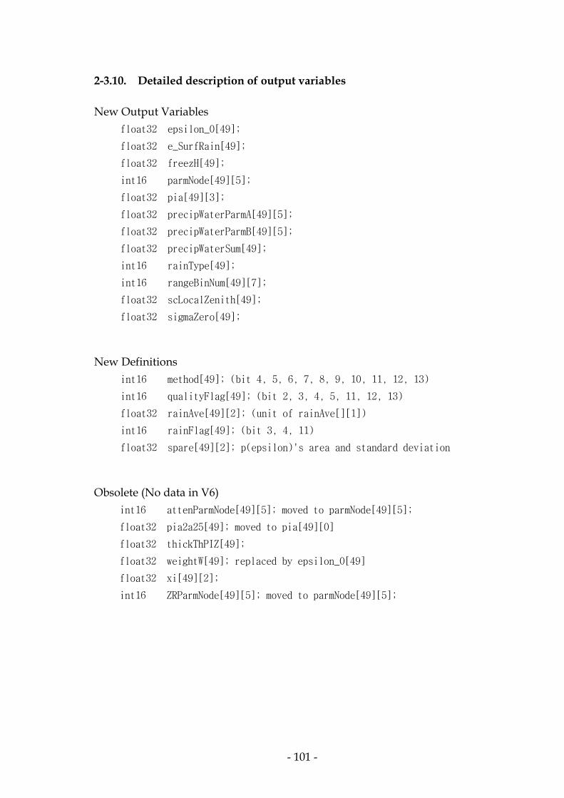
- 101 -
2-3.10. Detailed description of output variables New Output Variables
float32 epsilon_0[49];
float32 e_SurfRain[49];
float32 freezH[49];
int16 parmNode[49][5];
float32 pia[49][3];
float32 precipWaterParmA[49][5];
float32 precipWaterParmB[49][5];
float32 precipWaterSum[49];
int16 rainType[49];
int16 rangeBinNum[49][7];
float32 scLocalZenith[49];
float32 sigmaZero[49];
New Definitions
int16 method[49]; (bit 4, 5, 6, 7, 8, 9, 10, 11, 12, 13)
int16 qualityFlag[49]; (bit 2, 3, 4, 5, 11, 12, 13)
float32 rainAve[49][2]; (unit of rainAve[][1])
int16 rainFlag[49]; (bit 3, 4, 11)
float32 spare[49][2]; p(epsilon)'s area and standard deviation
Obsolete (No data in V6)
int16 attenParmNode[49][5]; moved to parmNode[49][5];
float32 pia2a25[49]; moved to pia[49][0]
float32 thickThPIZ[49];
float32 weightW[49]; replaced by epsilon_0[49]
float32 xi[49][2];
int16 ZRParmNode[49][5]; moved to parmNode[49][5];

- 102 -
List of 2A25 scan data float32 attenParmAlpha[49][5];
int16 attenParmAlpha_scale[49][5];
float32 attenParmBeta[49];
int16 attenParmBeta_scale[49];
int16 attenParmNode[49][5]; Obsolete
float32 correctZFactor[49][80];
int16 correctZFactor_scale[49][80];
float32 epsilon[49];
float32 epsilon_0[49]; New
float32 errorRain[49];
float32 errorZ[49];
float32 e_SurfRain[49]; New
float32 freezH[49]; New
float32 geolocation[49][2];
int16 method[49];
NAVIGATION navigate;
float32 nearSurfRain[49];
float32 nearSurfZ[49];
float32 nubfCorrectFactor[49][2];
int16 parmNode[49][5]; New
float32 pia[49][3]; New
float32 pia2a25[49]; Obsolete
float32 precipWaterParmA[49][5]; New
float32 precipWaterParmB[49][5]; New
float32 precipWaterSum[49]; New
int16 precipWaterSum_scale[49]; New
int16 qualityFlag[49];
float32 rain[49][80];
int16 rain_scale[49][80];
float32 rainAve[49][2];
int16 rainAve_scale[49][2];
int16 rainFlag[49];
int16 rainType[49]; New
int16 rangeBinNum[49][7]; Partly new
int8 reliab[49][80];
PR_SCAN_STATUS scanStatus;

- 103 -
float64 scanTime;
float32 scLocalZenith[49]; New
float32 sigmaZero[49]; New
float32 spare[49][2];
int16 thickThPIZ[49]; Obsolete
float32 weightW[49]; Obsolete
int16 weightW_scale[49]; Obsolete
float32 xi[49][2]; Obsolete
float32 zmmax[49];
float32 zeta[49][2];
float32 zeta_mn[49][2];
float32 zeta_sd[49][2];
int16 ZRParmA_scale[49][5];
float32 ZRParmA[49][5];
int16 ZRParmB_scale[49][5];
float32 ZRParmB[49][5];
int16 ZRParmNode[49][5]; Obsolete
Description of each output variable attenParmAlpha
float32 attenParmAlpha[49][5];
REAL*4 attenParmAlpha(5,49)
Internally this quantity is stored as
int16 attenParmAlpha_scale[49][5] after multiplied (scaled) by 10000000.
Attenuation parameter alpha at nodes.
k = alpha*Z^beta.
"alpha" is given at five nodal points. These numbers are initial values of alpha.
The mean values of alpha used in the attenuation correction are obtained by
multiplying attenParmAlpha[49][5] by epsilon[49].
The alpha values between the nodes are calculated by linear interpolation.
The range bin numbers of the nodes are stored in ParmNode[49][5]
(in version 5, they were stored in attenParmNode[49][5]).

- 104 -
attenParmBeta float32 attenParmBeta[49];
REAL*4 attenParmBeta(49)
Internally this quantity is stored as
int16 attenParmBeta_scale[49] after multiplied (scaled) by 10000.
Attenuation parameter beta
k = alpha*Z^beta.
beta is given for each angle bin.
A constant beta is used for all ranges in one angle bin. attenParmNode (Obsolete. No data in V6)
int16 attenParmNode[49][5];
INTEGER*2 attenParmNode(5,49);
This parameter gives the range bin numbers of the nodes where attanParmAlpha
and attenParmBeta are given. The numbers are stored in parmNode[49][5] in V6. correctZFactor
float32 correctZFactor[49][80];
REAL*4 correctZFactor(80,49)
Internally this quantity is stored as
int16 correctZFactor_scale[49][80] after multiplied (scaled) by 100.
Estimated effective Z-factor in dBZ at 13.8 GHz after attenuation correction.
If the input radar reflectivity factor Zm is below the noise level,
or if the estimate is below 0 dB, correctZFactor is set to 0.0.
Everythingelse is the same as rain[49][80] (rain(80,49)).
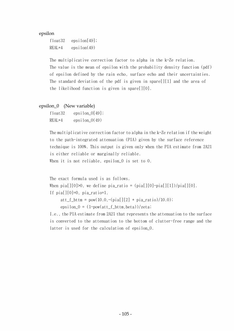
- 105 -
epsilon
float32 epsilon[49];
REAL*4 epsilon(49)
The multiplicative correction factor to alpha in the k-Ze relation.
The value is the mean of epsilon with the probability density function (pdf)
of epsilon defined by the rain echo, surface echo and their uncertainties.
The standard deviation of the pdf is given in spare[][1] and the area of
the likelihood function is given in spare[][0]. epsilon_0 (New variable)
float32 epsilon_0[49];
REAL*4 epsilon_0(49)
The multiplicative correction factor to alpha in the k-Ze relation if the weight
to the path-integrated attenuation (PIA) given by the surface reference
technique is 100%. This output is given only when the PIA estimate from 2A21
is either reliable or marginally reliable.
When it is not reliable, epsilon_0 is set to 0.
The exact formula used is as follows.
When pia[][0]>0, we define pia_ratio = (pia[][0]-pia[][1])/pia[][0].
If pia[][0]=0, pia_ratio=1.
att_f_bttm = pow(10.0,-(pia[][2] * pia_ratio)/10.0);
epsilon_0 = (1-pow(att_f_bttm,beta))/zeta;
I.e., the PIA estimate from 2A21 that represents the attenuation to the surface
is converted to the attenuation to the bottom of clutter-free range and the
latter is used for the calculation of epsilon_0.

- 106 -
errorRain
float32 errorRain[49];
REAL*4 errorRain(49)
Error estimate of rain rate near the surface expressed in dB.
The error is calculated as the standard deviation of the probability
distribution of rain rate derived from the pdf of epsilon. errorZ
float32 errorZ[49];
REAL*4 errorZ(49)
Error estimate of correctZFactor near the surface expressed in dB.
The error is calculated as the standard deviation of the probability
distribution of correctZFactor derived from the pdf of epsilon. e_SurfRain (New variable)
float32 e_SurfRain[49];
REAL*4 e_SurfRain(49)
Estimated rainfall rate at the actual surface. e_SurfRain is calculated by
assuming a constant slope of dBZe from the bottom of the valid (clutter-free)
rain echo. The assumed slope is 0 dB/km for all rain types except for the
stratiform rain over land where -0.5 dB/km toward the surface is assumed.
Note that 0 dB/km in Ze corresponds to -0.17 dB/km in rainfall rate (decreases
toward the surface). freezH (New variable)
float32 freezH[49];
REAL*4 freezH(49)
Freezing height expressed in m estimated from the climatological surface
temperature. This is a copy of freezH given in 2A23.(freezH in 2A23 is
given as an integer, but it is stored as a float number in 2A25.)

- 107 -
Note that the phase transition height used in 2A25 is different from
the freezing height given in freezH. In fact, when the bright band is detected,
its height is the phase transition height, and in other cases the phase
transition height is 1.2 times the height given in freezH. geolocation
float32 geolocation[49][2];
REAL*4 geolocation(2,49)
The earth location of the center of the IFOV at the altitude of the earth
ellipsoid. The first dimension is latitude and longitude, in that order.
Values are represented as floating point decimal degrees. Off-earth is
represented as -9999.9.
Latitude is positive north, negative south. Longitude is positive east,
negative west. A point on the 180° meridian is assigned to the western
hemisphere. method (New definition. bit 4, 5, 6, 7, 8, 9, 10, 11, 12, 13)
int16 method[49];
INTEGER*2 method(49)
Method (rain model) used in the retrieval of vertical profiles of Z and R
The default value is 0 (including no rain case).
The following meanings are assigned to each bit in the 16-bit integer.
(See flag_mthd) 0: (bit 1) no rain
if rain
0: (bit 1) over ocean
1: (bit 1) over land
2: (bit 2) over coast, river, etc.
3: (bit 2) others (impossible)
+4: (bit 3) PIA from constant-Z-near-surface assumption
+8: (bit 4) spatial reference
+16: (bit 5) temporal reference +32: (bit 6) global reference

- 108 -
+64: (bit 7) hybrid reference
+128: (bit 8) good to take statistics of epsilon.
+256: (bit 9) HB method used, SRT totally ignored
+512: (bit 10) very large pia_srt for given zeta
+1024: (bit 11) very small pia_srt for given zeta
+2048: (bit 12) no ZR adjustment by epsilon
+4096: (bit 13) no NUBF correction because NSD unreliable
+8192: (bit 14) surface attenuation > 60 dB
+16384: (bit 15) data partly missing between rain top and bottom
16th bit is currently not used.
The constant Z method is used only when the surface reference is unreliable.
This routine calculates the average slope of the Zm profile (expressed in dBZ)
near the bottom of radar echo and attributes the slope to the attenuation.
If there are not enough valid data points in the profile, it returns with
0 attenuation. The constant Z method is seldom used in V6. navigate
NAVIGATION navigate;
Look at the TSDIS INTERFACE CONTROL SPECIFICATION (ICS) Vol. 3,
Appendix B “Navigation” nearSurfRain
float32 nearSurfRain[49];
REAL*4 nearSurfRain(49)
Internally this quantity is stored as
int16 nearSurfRain_scale[49][80] after multiplied (scaled) by 100.

- 109 -
Near-surface rainfall rate estimate
"Near-surface" is defined as the lowest point in the clutter free ranges
in almost all cases. However, if Zm at this point is below the noise level
and if zeta which corresponds to the estimated attenuation down to this point
is larger than the zeta_th_L defined in the parameter file (it is currently
set to 0.7 which approximately corresponds to 4 dB of attenuation),
in other words,
if the first bit of reliab[][] = 0 and
if the forth bit of reliab[][] = 0,
then the lowest range bin at which Zm is above the noise threshold is chosen
as the near-surface range bin. The actual value of this near-surface range bin
is stored in rangeBinNum[][6] in V6.
Specifically,
nearSurfRain[n_anglebin] = rain[n_anglebin][rangeBinNum[n_anglebin][6]];
nearSurfRain(n_anglebin) = rain((rangeBinNum(7,n_anglebin)+1),n_anglebin) nearSurfZ
float32 nearSurfZ[49];
REAL*4 nearSurfZ(49)
Internally this quantity is stored as
int16 nearSurfZ_scale[49][80] after multiplied (scaled) by 100. Near-surface Z-factor
See nearSurfRain[] for the definition of "Near-surface".
nearSurfZ[n_anglebin]=
correctZFactor[n_anglebin][rangeBinNum[n_anglebin][6]];
nearSurfZ(n_anglebin)=
correctZFactor((rangeBinNum(7,n_anglebin)+1),n_anglebin)

- 110 -
nubfCorrectFactor
float32 nubfCorrectFactor[49][2];
REAL*4 nubfCorrectFactor(2,49)
'nubfCorrectFactor` is the non-uniform beam filling (NUBF) correction factor.
nubfCorrectFactor[][0] is the NUBF correction factor for the surface reference
and its range is between 1.0 and 3.0.
nubfCorrectFactor[][1] is the NUBF correction factor for the Z-R relation and
its range is between 0.8 and 1.0.
N.B. No NUBF correction is made in V6. As a result, both nubfCorrectFactor[][0]
and nubfCorrectFactor[][1] are always set to 0 in V6. parmNode (New variable)
int16 parmNode[49][5];
INTEGER*2 parmNode(5,49)
Range bin numbers of the nodal points at which
the attenuation parameter alpha and the Z-R parameters "a" and "b" are given
in attenParmAlpha[49][5] (attenParmAlpha(5,49)),
ZRParmA[49][5] (ZRParmA(5,49)), and
ZRParmB[49][5] (ZRParmB(5,49)), respectively.
For each angle bin, 5 nodal points are defined.
ParmNode[][] gives the range bin numbers of the 5 nodes at which
the values of attenuation parameter "alpha" and the Z-R parameters "a" and "b"
are given in ParmAlpha[][], ZRParmA[][] and ZRParmB[][], respectively.
The values of alpha, a and b between the nodes are linearly interpolated.
The range of ParmNode is between 0 and 79. (See the note for rangeBinNum.)
In no-rain angle bins, ParmNode[][] is set to 0.
Note that the definition of range bin number in 2A25 is not the same as
1B-21 or 1C-21. The bin number shows the position in the 80-element array
so that it takes a number between 0 and 79 (inclusive).
Bin number 79 corresponds to the surface of the ellipsoid which is approximately
equal to the sea surface.

- 111 -
pia (New variable)
float32 pia[49][3];
REAL*4 pia(3,49)
pia[][0]
Path-integrated attenuation from rain top to surface.
This attenuation is calculated from the attenuation-corrected Z-profile
in correctZFactor[][] and adjusted alpha.
The number represents the two-way attenuation to the actual surface.
pia[][1]
Path-integrated attenuation between the clutter-free bottom and the surface.
This is the attenuation estimate in the range that is cluttered by the surface
echo.
pia[][2]
Path-integrated attenuation to surface estimated by the surface reference
technique in 2A21. This is an exact copy of pathAtten(49) in 2A21. pia2a25 (Obsolete, No data in V6) moved to pia[49][0] in version 6.
float32 pia2a25[49];
REAL*4 pia2a25(49)
Path-integrated attenuation from the estimated Z profile

- 112 -
precipWaterParmA (New variable)
float32 precipWaterParmA[49][5];
READ*4 precipWaterParmA(5,49)
Coefficient a in the relation between the precipitation water content (PWC)
and Ze at 5 nodal points. The unit of PWC is g/m^3 and that of Ze is mm^6/m^3.
PWC = a*Z^b.
'a' is given at five nodal points.
These values are stored in the first 5 elements of the array.
'a' values between the nodes can be calculated by linear interpolation.
The range bin numbers of the nodes are stored in the ParmNode[49][5]
(ParmNode(5,49)).
Note that the sum of PWC’s calculated from Z=correctZFactor with formula
PWC = a*Z^b where a and b from the interpoloted values of precipWaterParmA
and precipWaterParmB does not necessarily agree with precipWaterSum.
The former is <a>*<Z>^<b> where as the latter is <a*Z^b>. precipWaterSum
also includes the precipitation water content in the surface clutter range. precipWaterParmB (New variable)
float32 precipWaterParmB[49][5];
READ*4 precipWaterParmB(5,49)
Coefficient a in the relation between the precipitation water content (PWC)
and Ze at 5 nodal points. The unit of PWC is g/m^3 and that of Ze is mm^6/m^3.
PWC = a*Z^b.
'b' is given at five nodal points.
'b' values between the nodes can be calculated by linear interpolation.
The range bin numbers of the nodes are stored in the ParmNode[49][5]
(ParmNode(5,49)).

- 113 -
precipWaterSum (New variable)
float32 precipWaterSum[49];
REAL*4 precipWaterSum(49)
Internally this quantity is stored as
int16 precipWaterSum_scale[49] after multiplied (scaled) by 1000.
Vertically integrated value of precipitation water content.
The unit is g km/m^3 or equivalently kg/m^2.
“precipWaterSum” give the sum of the precipitation water content calculated
from Ze at each range bin. The summation is from the rain top to the actual
surface. The water content in the surface clutter range is estimated with the
same assumption that is used in the attenuation correction.The sum includes
both liquid and solid phase regions. qualityFlag (New definition, bit 2, 3, 4, 5, 11, 12, 13)
int16 qualityFlag[49];
INTEGER*2 qualityFlag(49)
Quality flag for each angle bin data
The default value is 0.
In V6, the definitions of bits 2, 3, 4, 5 are changed, and bits 13 and 14 are
added. The flags indicated by bits 4, 5 and 13 in V6 are moved from method flag
in V5. 0: normal
+1: unusual situation in rain average
+2: NSD of zeta (xi) calculated from less than 6 points
+4: NSD of PIA calculated from less than 6 points
+8: NUBF for Z-R below lower bound
+16: NUBF for PIA above upper bound
+32: epsilon not reliable, epsi_sig <= 0.0
+64: 2A21 input data not reliable
+128: 2A23 input data not reliable
+256: range bin error
+512: sidelobe clutter removal
+1024: probability=0 for all tau
+2048: pia_surf_ex <= 0.0

- 114 -
+4096: const Z is invalid
+8192: reliabFactor in 2A21 is NaN
+16384: data missing 16th bit (sign bit) is not used.
The contents are exact copy of internal variable flag_qlty. rain
float32 rain[49][80];
REAL*4 rain(80,49)
Internally this quantity is stored as
int16 rain_scale[49][80] after multiplied (scaled) by 100.
rainfall rate in mm/h
49 elements in the 2-D array correspond to the angle bins and 80 elements
(first argument in FORTRAN convention) in the 2-D array correspond to the range
bins.
If the estimated Z-factor is below 0 dBZ, the rain rate is always set to 0.
If the input radar reflectivity factor Zm is below the noise level,
the corresponding rain estimate is set to 0. This procedure does not cause
any serious problem except when the measured Zm becomes smaller than the noise
level by rain attenuation. In such a case, even if some heavy rain exists near
the surface,the number in this variable is 0.
To know whether such low radar reflectivity factors are caused by large
attenuation or not, look at the forth bit of 'reliab' and the forth bit of
rainFlag.
80 range bins are filled with data from top to bottom in height.
The last element corresponds to the ellipsoid height, i.e., 0 m high above
the model ellipsoid (not the actual surface). The first element corresponds
to the radar resolution cell about 20 km above in slant range along the beam
from the footprint on the ellipsoid. The range resolution is 250 m.

- 115 -
If the radar data is missing, MISSING value of -99.99 is stored.
This situation may happen at range bins above 15 km high because JAXA only
guarantees the data collection below 15km.
(The highest edge of the radar's receiving window comes down to nearly 15km
above the sea level near the equator.)
The bin number of the lowest range bin that contains valid rain data is
(rangeBinNum[][6] - 1 in C) or (rangeBinNum(7,.) - 1 in FORTRAN).
Below this level, CLUTTER value of -88.88 is stored.
If the estimated rainfall rate exceeds 300 mm/h, it is reset to 300 mm/h.
In V6, this reset is made before the mean of the distribution is calculated
so that the mean never reaches 300 mm/h. If the substantial part of
the distribution exceeds this threshold, a flag in flagRain is set.
(The rainfall rate that corresponds to the epsilon at which the pdf p(epsilon)
becomes one tenth of the maximum of p(epsilon) is larger than 300 mm/h,
the flag is set.) rainAve (New definition)
float32 rainAve[49][2];
REAL*4 rainAve(2,49)
Internally this quantity is stored as
int16 rainAve_scale[49][2] after multiplied (scaled) by 100.
rainAve[][0] :
rainAve(1,*) : Average of rainfall rate between 2 and 4 km. The unit is mm/h.
If the lowest bin processed is higher than 2 km, the average is taken between the lowest altitude and 4 km.In this case, the 6th bit in rainFlag is set.
If the lowest bin processed is higher than 4 km, the average is not calculated.
In this case, 0 is stored, and the seventh bit of rainFalg is set.
rainAve[][1] :
rainAve(2,*) : Integrated rainfall rate from the rain top to the bottom.
The new unit in V6 is (cm/h)*km, and NOT (mm/h)*km. This odd unit is adopted
to avoid the overflow when the sum is stored as int16 after scaled by 100.
(It is not possible to use different scale factors for rainAve[][0]
and rainAve[][1]. Cases with overflow were found in V5.)
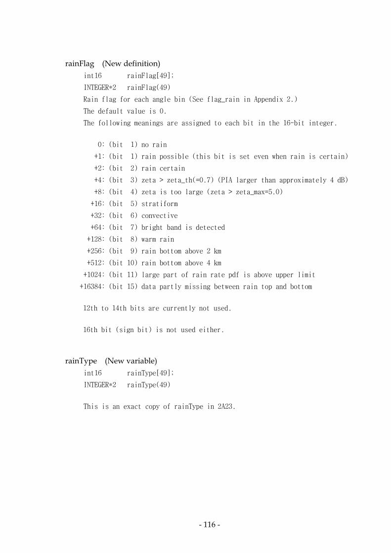
- 116 -
rainFlag (New definition)
int16 rainFlag[49];
INTEGER*2 rainFlag(49)
Rain flag for each angle bin (See flag_rain in Appendix 2.)
The default value is 0.
The following meanings are assigned to each bit in the 16-bit integer.
0: (bit 1) no rain
+1: (bit 1) rain possible (this bit is set even when rain is certain)
+2: (bit 2) rain certain
+4: (bit 3) zeta > zeta_th(=0.7) (PIA larger than approximately 4 dB)
+8: (bit 4) zeta is too large (zeta > zeta_max=5.0)
+16: (bit 5) stratiform
+32: (bit 6) convective
+64: (bit 7) bright band is detected
+128: (bit 8) warm rain
+256: (bit 9) rain bottom above 2 km
+512: (bit 10) rain bottom above 4 km
+1024: (bit 11) large part of rain rate pdf is above upper limit
+16384: (bit 15) data partly missing between rain top and bottom
12th to 14th bits are currently not used.
16th bit (sign bit) is not used either.
rainType (New variable)
int16 rainType[49];
INTEGER*2 rainType(49)
This is an exact copy of rainType in 2A23.

- 117 -
rangeBinNum (New definition)
int16 rangeBinNum[49][7];
INTEGER*2 rangeBinNum(7,49)
rangeBinNum[][0]: range bin number at the top of the interval
that is processed as meaningful data in 2A-25.
This is 4 range bins (1 km) above the first (highest)
rain-certain range bin.
rangeBinNum[][1]: range bin number at the top of the surface clutter
defined in 1B21.
rangeBinNum[][2]: range bin number at the actual surface.
rangeBinNum[][3]: range bin number of the bright band if it exits.
If not, the range bin number of the phase transition height
(estimated 0C height) is stored. (Read the note for freezH.)
rangeBinNum[][4]: the range bin number at which the path-integrated Z-factor
first exceeds the given threshold. If the path-integrated
Z-factor does not exceed the threshold, it is set to 79.
rangeBinNum[][5]: the range bin number at which the measured Z-factor is
maximum. If no rain, it is set to 79.
rangeBinNum[][6]: the range bin number at the bottom of the interval that is
processed as meaningful data in 2A-25.
The attenuation-corrected Ze and rainfall rate R at this
range bin are defined as nearSurfZ and nearSurfRain.
See note below.
All these range bin numbers are indexed vertically from top to bottom with 0
at the highest elevation and 79 at the earth ellipsoid.
(All negative bin numbers are set to 0, and numbers larger than 79 are set to
79.)
Exception: If the actual surface is lower than the ellipsoid, the number in
rangeBinNum[][2] may be larger than 79. This situation happens occasionally,
especially over Indian Ocean where the geoid surface is lower than the model
ellipsoid. The same situation may happen at a very low place over land, for
example, at Dead Sea where the surface is nearly 400 m below the sea level.
Range bin numbers are unitless.

- 118 -
Note 1: rangeBinNum[][1] contains the range bin number that is the top of the
possibly surface cluttered ranges. This number is larger than the bin number
for the bottom of the clutter-free ranges by one.
Note 2: rangeBinNum[][6] contains the range bin number that corresponds to the
bottom of the interval that is processed as meaningful data in 2A-25. This range
bin is one bin above the top of the region that is cluttered either by the surface
echo in the antenna mainlobe or by noise. In the former case, this number is
identical to (rangeBinNum[][1]-1), but in the latter case, rangeBinNum[][6]
is different from (rangeBinNum[][1]-1). The latter case may happen when the
rain echo near surface becomes lower than the noise level by very large
attenuation due to heavy rain. When rain is light and the echo near surface
is below the noise level, the data smaller than the noise level are treated
as valid data and the rainfall rate at that bin is set to zero.
reliab
int8 reliab[49][80];
BYTE reliab(80,49)
Reliability parameter at each range bin
The default value is 0.
Each bit in the byte indicates the status shown below:
lowest (first) bit : 0 : measured signal below noise
lowest (first) bit : rain
second bit : rain certain
third bit : bright band
forth bit : large attenuation
fifth bit : weak return (Zm < 20 dBZ)
sixth bit : estimated Z < 0 dBZ
seventh bit : main-lobe clutter or below surface
eighth bit : missing data
For example, if the first bit is 0, i.e., if the number is an even number,
then the measured signal in that range bin is below the noise level
(noise threshold).

- 119 -
The large attenuation flag is set below the height at which the integral of
0.2*ln(10)*beta*alpha*Zm^beta first exceeds the given threshold.
In the version 6, the threshold is chosen that approximately corresponds to
the attenuation of 4 dB.
scanStatus
PR_SCAN_STATUS scanStatus;
See the description of the 1B21 Scan Status in the TSDIS INTERFACE CONTROL
SPECIFICATION (ICS) Volume 3.
scanTime
float64 scanTime;
REAL*8 scanTime
See the description of the 1B21 Scan Status in the TSDIS INTERFACE CONTROL
SPECIFICATION (ICS) Volume 3.
scLocalZenith (New variable)
float32 scLocalZenith[49];
REAL*4 scLocalZenith(49)
Local zenith angle of the satellite at the center of the footprint.
The number corresponds to the incidence angle of the radar beam to the surface
(ellipsoid surface).
sigmaZero (New variable)
float32 sigmaZero[49];
REAL*4 sigmaZero(49)
Exact copy of sigmaZero from 2A21.

- 120 -
spare (New definition)
float32 spare[49][2];
REAL*4 spare(2,49)
spare[49][0] : area of the likelihood function of epsilon.
spare[49][1] : standard deviation of the probability distribution function
(pdf) of epsilon.
thickThPIZ (Obsolete. No data in V6)
int16 thickThPIZ[49];
INTEGER*2 thickThPIZ(49)
weightW (Obsolete. No data in V6. Can be calculated from epsilon and epsilon_0.)
float32 weightW[49];
REAL*4 weightW(49)
Internally this quantity was stored as
int16 weightW_scale[49] after multiplied (scaled) by 1000.
Weighting factor in the calculation of epsilon (SRT correction factor)
in the hybrid method. The number is always between 0 and 1 (inclusive).
Note that in V6, epsilon_0 is output instead of weightW.
The relationship among epsilon, epsilon_0 and weightW is as follows.
epsilon = 1 + weightW*(epsilon_0 - 1)

- 121 -
xi (Obsolete. No data in V6. Can be calculated from zeta_sd and zeta_mn.)
float32 xi[49][2];
REAL*4 xi(2,49)
Normalized standard deviation of zeta and PIA_est
xi[][0]: xi = zeta_sd/zeta_mn
xi[][1]: nsd_l = normalized standard deviation of pia_est
When zeta_mn is less than 0.01, xi[][0] is set to 0.
When pia_mn is less than 0.1, zi[][1] is set to 0.
xi is unitless.
zeta
float32 zeta[49][2];
REAL*4 zeta(2,49)
Integral of 0.2*ln(10)*beta*alpha*Z^beta from rain top to the clutter-free
bottom.
zeta[][0]: zeta = Integral of 0.2*ln(10)*beta*alpha*Z^beta from the rain top
to the bottom (lowest altitude processed).
zeta[][1]: PIA_est = -10*(log10(1-zeta_cr))/beta where zeta_cr is a corrected
zeta (This zeta_cr is calculated by using the value of
epsilon in the first cycle of processing which is different
from the final estimate of epsilon.).
zeta is always between 0 and 100, typically between 0 and 2. When it is larger
than 5, the 4th bit of rainFlag is set.
zeta is unitless.

- 122 -
zeta_mn
float32 zeta_mn[49][2];
REAL*4 zeta_mn(2,49)
Mean of zeta and PIA of 9 adjacent (3x3) beams.
At scan edges, the mean is calculated of 6 beams. At the scan edges of the first
and last scans of the granule, the mean is calculated from only 4 beams.
zeta_mn[][0]: zeta_mn = mean of zeta
zeta_mn[][1]: PIA_mn = mean of PIA_est
The range of output value is the same as zeta itself.
zeta_mn is unitless.
zeta_sd
float32 zeta_sd[49][2];
REAL*4 zeta_sd(2,49)
Standard deviation of zeta and PIA_est in 9 adjacent (3 x 3) beams.
At scan edges, it is calculated in 6 beams. At the scan edges of the first and
last scans of the granule, the mean is calculated from only 4 beams.
zeta_sd[][0]: zeta_sd = standard deviation of zeta
zeta_sd[][1]: PIA_sd = standard deviation of pia_est
zeta_sd is unitless.
zmmax
float32 zmmax[49];
REAL*4 zmmax(49)
zmmax is the maximum value of measured Z-factor expressed in dBZ at each IFOV.
The unit is dBZ or 10 log of mm^6/m^3. The range of the variable is between
0 and 100. (Typically between 10 and 60.)

- 123 -
ZRParmA
float32 ZRParmA[49][5];
REAL*4 ZRParmA(5,49)
Internally this quantity is stored as
int16 ZRParmA_scale[49][5] after multiplied (scaled) by 100000.
Z-R parameter 'a' at nodal points.
R = a*Z^b.
'a' is given at five nodal points.
These values are stored in the first 5 elements of the array.
'a' values between the nodes are calculated by linear interpolation.
The range bin numbers of the nodes are stored in ParmNode[49][5]
(ParmNode(5,49)).
ZRParmB
float32 ZRParmB[49][5];
REAL*4 ZRParmB(5,49)
Internally this quantity is stored as
int16 ZRParmB_scale[49][5] after multiplied (scaled) by 10000.
Z-R parameter 'b' at nodal points.
R = a*Z^b.
'b' is given at five nodal points.
The nodal points are the same as those for alpha.
'b' values between the nodes are calculated by linear interpolation.
The range bin numbers of the nodes are stored in ParmNode[49][5]
(ParmNode(5,49)).
ZRParmNode (Obsolete. No data in V6)
int16 ZRParmNode[49][5];
INTEGER*2 ZRParmNode(5,49);
This parameter is absorbed in parmNode[49][5].

- 124 -
Appendix 1. Output data structure defined in the toolkit /****************************************/
/* Define L2A-25 data structure. */
/****************************************/
typedef struct
{
int8 mainlobeEdge;
int8 sidelobeRange[3];
} CFLAGS;
typedef struct
{
CFLAGS clutFlag[CLUTFLAG_TBL_SIZE];
} CLUTTER_FLAGS;
typedef struct
{
float64 scanTime;
float32 geolocation[49][2];
PR_SCAN_STATUS scanStatus;
NAVIGATION navigate;
float32 scLocalZenith[49];
int16 rain_scale[49][80];
float32 rain[49][80];
int8 reliab[49][80];
int16 correctZFactor_scale[49][80];
float32 correctZFactor[49][80];
int16 attenParmNode[49][5];
int16 attenParmAlpha_scale[49][5];
float32 attenParmAlpha[49][5];
int16 attenParmBeta_scale[49];
float32 attenParmBeta[49];
int16 ZRParmNode[49][5];
int16 parmNode[49][5];
float32 precipWaterParmA[49][5];
float32 precipWaterParmB[49][5];
int16 ZRParmA_scale[49][5];
float32 ZRParmA[49][5];

- 125 -
int16 ZRParmB_scale[49][5];
float32 ZRParmB[49][5];
float32 zmmax[49];
int16 rainFlag[49];
int16 rangeBinNum[49][7];
int16 rainAve_scale[49][2];
float32 rainAve[49][2];
int16 precipWaterSum_scale[49];
float32 precipWaterSum[49];
int16 weightW_scale[49];
float32 weightW[49];
float32 epsilon_0[49];
int16 method[49];
float32 epsilon[49];
float32 zeta[49][2];
float32 zeta_mn[49][2];
float32 zeta_sd[49][2];
float32 xi[49][2];
float32 sigmaZero[49];
float32 freezH[49];
int16 thickThPIZ[49];
float32 nubfCorrectFactor[49][2];
int16 qualityFlag[49];
float32 nearSurfRain[49];
float32 nearSurfZ[49];
float32 pia2a25[49];
float32 e_SurfRain[49];
float32 pia[49][3];
float32 errorRain[49];
float32 errorZ[49];
float32 spare[49][2];
int16 rainType[49];
} L2A_25_SWATHDATA;
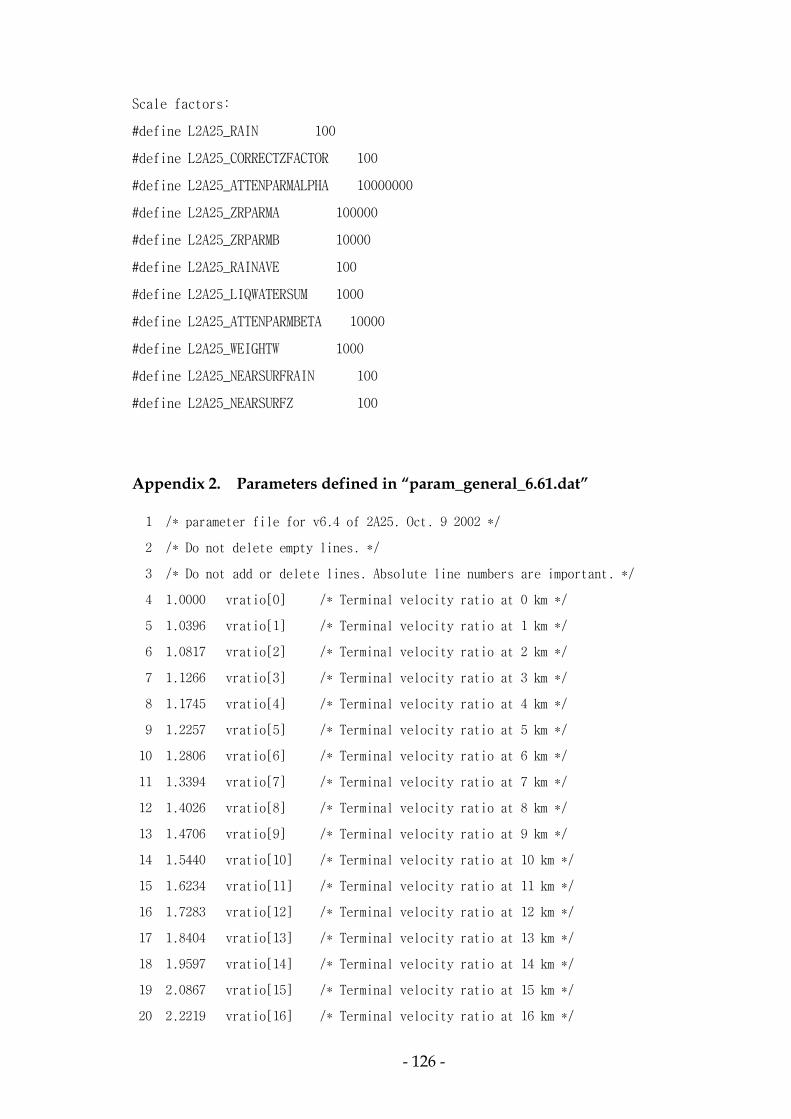
- 126 -
Scale factors:
#define L2A25_RAIN 100
#define L2A25_CORRECTZFACTOR 100
#define L2A25_ATTENPARMALPHA 10000000
#define L2A25_ZRPARMA 100000
#define L2A25_ZRPARMB 10000
#define L2A25_RAINAVE 100
#define L2A25_LIQWATERSUM 1000
#define L2A25_ATTENPARMBETA 10000
#define L2A25_WEIGHTW 1000
#define L2A25_NEARSURFRAIN 100
#define L2A25_NEARSURFZ 100
Appendix 2. Parameters defined in “param_general_6.61.dat” 1 /* parameter file for v6.4 of 2A25. Oct. 9 2002 */
2 /* Do not delete empty lines. */
3 /* Do not add or delete lines. Absolute line numbers are important. */
4 1.0000 vratio[0] /* Terminal velocity ratio at 0 km */
5 1.0396 vratio[1] /* Terminal velocity ratio at 1 km */
6 1.0817 vratio[2] /* Terminal velocity ratio at 2 km */
7 1.1266 vratio[3] /* Terminal velocity ratio at 3 km */
8 1.1745 vratio[4] /* Terminal velocity ratio at 4 km */
9 1.2257 vratio[5] /* Terminal velocity ratio at 5 km */
10 1.2806 vratio[6] /* Terminal velocity ratio at 6 km */
11 1.3394 vratio[7] /* Terminal velocity ratio at 7 km */
12 1.4026 vratio[8] /* Terminal velocity ratio at 8 km */
13 1.4706 vratio[9] /* Terminal velocity ratio at 9 km */
14 1.5440 vratio[10] /* Terminal velocity ratio at 10 km */
15 1.6234 vratio[11] /* Terminal velocity ratio at 11 km */
16 1.7283 vratio[12] /* Terminal velocity ratio at 12 km */
17 1.8404 vratio[13] /* Terminal velocity ratio at 13 km */
18 1.9597 vratio[14] /* Terminal velocity ratio at 14 km */
19 2.0867 vratio[15] /* Terminal velocity ratio at 15 km */
20 2.2219 vratio[16] /* Terminal velocity ratio at 16 km */

- 127 -
21 2.3658 vratio[17] /* Terminal velocity ratio at 17 km */
22 2.5189 vratio[18] /* Terminal velocity ratio at 18 km */
23 2.6819 vratio[19] /* Terminal velocity ratio at 19 km */
24 2.8554 vratio[20] /* Terminal velocity ratio at 20 km */
25 0.075 lprate /* 1/20 of the lapse rate per 250 m */
26 1.2 fhcf /* Freezing height correction factor */
27 0.3 nsd_cnv[0] /* Conv. factor of NSD for stratiform: was 0.3 */
28 0.5 nsd_cnv[1] /* Conv. factor of NSD for convective: was 0.5 */
29 0.4 nsd_cnv[2] /* Conv. factor of NSD for default: was 0.4 */
30 0.0000 nubf_cf[0] /* Conv. coefficients for nubfCFs: was 1.30 */
31 0.0000 nubf_cf[1] /* nubfCFs = 1 + nubf_cf[0]*NSD^2 */
32 0.00 nubf_cf[2] /* nubf_cf[1]*NSD^2*PIA_a */
33 0.00 nubf_cf[3] /* Conv. coefficients for nubfCFzr: was 0.17 in V5 */
34 0.10 zeta_min /* Threshold value of zeta for SRT */
35 5.00 zeta_max /* Threshold for zeta to judge something wrong. */
36 0.70 zeta_th_L /* Threshold for zeta to judge large attenuation. */
37 0.00 z_offset /* Offset to be added to 1C21 Z factor in dB */
38 0.00 z_slope[0][0] /* Slope for ocean strat in clutter. + for larger Z toward surf. */
39 0.00 z_slope[0][1] /* Slope of dBZ/km for ocean conv. in cluttered range */
40 0.00 z_slope[0][2] /* Slope of dBZ/km for ocean others in cluttered range */
41 -0.50 z_slope[1][0] /* Slope of dBZ/km for land strat in clutter. */
42 0.00 z_slope[1][1] /* Slope of dBZ/km for land conv. in cluttered range */
43 0.00 z_slope[1][2] /* Slope of dBZ/km for land others in cluttered range */
44 1.00 epsi_init[0][0] /* initial offset factor of epsilon for ocean stratiform rain */
45 1.00 epsi_init[0][1] /* initial offset factor of epsilon for ocean convective rain */
46 1.00 epsi_init[0][2] /* initial offset factor of epsilon for ocean other rain */
47 1.00 epsi_init[1][0] /* initial offset factor of epsilon for land stratiform rain */
48 1.00 epsi_init[1][1] /* initial offset factor of epsilon for land convective rain */
49 1.00 epsi_init[1][2] /* initial offset factor of epsilon for land other rain */
50 0.08 atten_O2_surf /* PIA due to O2 at 0 m from geoid */
51 7.70 scale_h_O2 /* scale height of O2 in km */
52 90.0 r_humid_in_rain /* relative humidity inside the raining area */
53 70.0 r_humid_out_rain /* relative humidity outside the raining area */
54 2.00 scale_h_H2O /* scale height of H2O in km */

- 128 -
Appendix 3. Parameters defined in “param_error_6.61.dat” Note that many of the parameters defined in this file are not used in V6.
The parameters marked with “n” are not used.
01 0.7 d_Zm_typ /* Typical error (offset) in Zm in dB */ o
02 0.5 d_alpha_typ /* Typical error in alpha in dB */ n
03 0.05 d_beta_typ /* Typical error in beta in dB */ n
04 0.6 d_zra_typ /* Typical error in a in dB */ o
05 0.05 d_zrb_typ /* Typical error in b in dB */ o
06 1.5 d_surf_typ /* Typical error in sigma^0 in dB */ n
07 1.0 d_nubfCf_s /* Typical error in NUBF correct. factor for surf.*/ n
08 0.2 d_nubfCf_zr /* Typical error in NUBF correct. factor for ZR */ o
09 -0.2 dv_dh /* Typical change of velocity per km in dB*/ n
10 1.0 height_err_0C /* 0C height error in km */ o
11 0.3 height_err_BB /* BB height error in km when it exists */ o
12 -0.07 dalpha_dT /* Change of alpha per 1 degree in dB */ n
13 0.01 dbeta_dT /* Change of beta per degree in dB */ n
14 0.02 da_dT /* Change of a in ZR per degree in dB */ o
15 -0.005 db_dT /* Change of b in ZR per degree in dB */ o
16 1.3 d_alpha_id /* Error in alpha in dB caused by wrong ident. */ n
17 -0.05 d_beta_id /* Error in beta in dB caused by wrong ident. */ n
18 2.00 d_zra_id /* Error in a in dB caused by wrong identification */ o
19 0.02 d_zrb_id /* Error in b in dB caused by wrong identification */ o
20 0.4 stddev_epsi_strat /* nominal error of epsilon for strat in linear unit */o
21 0.3 stddev_epsi_conv /* nominal error of epsilon for conv in linear unit */o
22 0.7 stddev_SRT_O /* nominal error of SRT over ocean in dB */ o
23 2.2 stddev_SRT_L /* nominal error of SRT over land in dB */ o
24 5.0 stddev_SRT_N /* nominal error of SRT in const-Z method in dB */ o

- 129 -
Appendix 4. Parameters defined in “param_strat_1.dat” 1 /* parameter file for v6 of 2A25. June 13, 2001 */
2 /* Do not delete empty lines. */
3 /* Do not add or delete lines. Absolute line numbers are important. */
4 /* stratiform parameters */
5 /* coefficients for R-Z relationship: R = a * Z^b
6 log10(a) = zr_a_c0 + zr_a_c1*x + zr_a_c2*x*x
7 log10(b) = zr_b_c0 + zr_b_c1*x + zr_b_c2*x*x
8 where x = log10(alpha_final/alpha_initial) */
9 /* initial coefficients of k-Z relationship: k = alpha * Z^beta */
10 0.0000861 alpha_init[0][0] /* alpha for low density snow, bb.011, strat */
11 0.0001084 alpha_init[0][1] /* alpha for high density snow, bb.017, strat */
12 0.0004142 alpha_init[0][2] /* alpha for bright band peak, bb.17, strat */
13 0.0002822 alpha_init[0][3] /* alpha for rain (stratiform) 0C */
14 0.0002851 alpha_init[0][4] /* alpha for rain (stratiform) 20C */
15 0.79230 beta_init[0] /* beta for stratiform column, strat */
16 /* R-Ze coefficients */
17 -1.8545 zr_a_c0[0][0] /* stratiform, bb.011, a'= 251.0 */
18 -1.8985 zr_a_c0[0][1] /* stratiform, bb.017, a'= 304.3 */
19 -2.3448 zr_a_c0[0][2] /* stratiform, bb.17, a'=1648.4 */
20 -1.6969 zr_a_c0[0][3] /* stratiform, 0C , a'= 284.3 */
21 -1.6416 zr_a_c0[0][4] /* stratiform, 20C, a'= 276.1 */
22
23 1.6263 zr_a_c1[0][0] /* stratiform, bb.011 */
24 1.6041 zr_a_c1[0][1] /* stratiform, bb.017 */
25 1.4259 zr_a_c1[0][2] /* stratiform, bb.17 */
26 0.9367 zr_a_c1[0][3] /* stratiform, 0C */
27 0.9567 zr_a_c1[0][4] /* stratiform, 20C */
28
29 -0.2734 zr_a_c2[0][0] /* stratiform, bb.011 */
30 -0.2797 zr_a_c2[0][1] /* stratiform, bb.017 */
31 -0.4191 zr_a_c2[0][2] /* stratiform, bb.17 */
32 -0.7720 zr_a_c2[0][3] /* stratiform, 0C */
33 -1.9319 zr_a_c2[0][4] /* stratiform, 20C */
34
35 -0.1119 zr_b_c0[0][0] /* stratiform, bb.011, b=0.7729, 1/b=1.294 */
36 -0.1167 zr_b_c0[0][1] /* stratiform, bb.017, b=0.7644, 1/b=1.308 */
37 -0.1374 zr_b_c0[0][2] /* stratiform, bb.17, b=0.7288, 1/b=1.372 */
38 -0.1601 zr_b_c0[0][3] /* stratiform, 0C , b=0.6917, 1/b=1.446 */
39 -0.1722 zr_b_c0[0][4] /* stratiform, 20C, b=0.6727, 1/b=1.487 */
40
41 -0.1040 zr_b_c1[0][0] /* stratiform, bb.011 */
42 -0.0907 zr_b_c1[0][1] /* stratiform, bb.017 */

- 130 -
43 -0.0235 zr_b_c1[0][2] /* stratiform, bb.17 */
44 +0.0996 zr_b_c1[0][3] /* stratiform, 0C */
45 +0.1116 zr_b_c1[0][4] /* stratiform, 20C */
46
47 0.1327 zr_b_c2[0][0] /* stratiform, bb.011 */
48 0.1275 zr_b_c2[0][1] /* stratiform, bb.017 */
49 0.1118 zr_b_c2[0][2] /* stratiform, bb.17 */
50 0.2811 zr_b_c2[0][3] /* stratiform, 0C */
51 0.4095 zr_b_c2[0][4] /* stratiform, 20C */
52 /* LWC-Ze coefficients (log10 of a and b in LWC = a Ze^b) */
53 -2.4161 zl_a_c0[0][0] /* stratiform, bb.011, a=0.00383613 */
54 -2.4881 zl_a_c0[0][1] /* stratiform, bb.02, a=0.00325046 */
55 -3.1290 zl_a_c0[0][2] /* stratiform, bb.17, a=0.00074301 */
56 -2.6994 zl_a_c0[0][3] /* stratiform, 0C , a=0.00199806 */
57 -2.6502 zl_a_c0[0][4] /* stratiform, 20C , a=0.00223787 */
58
59 1.5422 zl_a_c1[0][0] /* stratiform, bb.011 */
60 1.8509 zl_a_c1[0][1] /* stratiform, 0C */
61 1.8344 zl_a_c1[0][2] /* stratiform, 0C */
62 1.5283 zl_a_c1[0][3] /* stratiform, 0C */
63 1.5422 zl_a_c1[0][4] /* stratiform, 20C */
64
65 -0.2365 zl_a_c2[0][0] /* stratiform, bb.011 */
66 -0.2254 zl_a_c2[0][1] /* stratiform, 0C */
67 -0.3571 zl_a_c2[0][2] /* stratiform, 0C */
68 -0.5889 zl_a_c2[0][3] /* stratiform, 0C */
69 -1.6158 zl_a_c2[0][4] /* stratiform, 20C */
70
71 -0.1471 zl_b_c0[0][0] /* stratiform, bb.011, b=0.71266 */
72 -0.1520 zl_b_c0[0][1] /* stratiform, bb.02, b=0.70472 */
73 -0.1768 zl_b_c0[0][2] /* stratiform, bb.17, b=0.66564 */
74 -0.2122 zl_b_c0[0][3] /* stratiform, 0C, b=0.61342 */
75 -0.2243 zl_b_c0[0][4] /* stratiform, 20C, b=0.59658 */
76
77 -0.1056 zl_b_c1[0][0] /* stratiform, bb.011 */
78 -0.0915 zl_b_c1[0][1] /* stratiform, 0C */
79 -0.0442 zl_b_c1[0][2] /* stratiform, 0C */
80 0.0630 zl_b_c1[0][3] /* stratiform, 0C */
81 0.0751 zl_b_c1[0][4] /* stratiform, 20C */
82
83 0.1453 zl_b_c2[0][0] /* stratiform, bb.011 */
84 0.1357 zl_b_c2[0][1] /* stratiform, 0C */
85 0.1265 zl_b_c2[0][2] /* stratiform, 0C */
86 0.1913 zl_b_c2[0][3] /* stratiform, 0C */
87 0.4320 zl_b_c2[0][4] /* stratiform, 20C */

- 131 -
Appendix 5. Parameters defined in “param_conv_1.dat” 1 /* parameter file for v6 of 2A25. June 13, 2001 */
2 /* Do not delete empty lines. */
3 /* Do not add or delete lines. Absolute line numbers are important. */
4 /* convective rain parameters */
5 /* coefficients for R-Z relationship: R = a * Z^b
6 log10(a) = zr_a_c0 + zr_a_c1*x + zr_a_c2*x*x
7 log10(b) = zr_b_c0 + zr_b_c1*x + zr_b_c2*x*x
8 where x = log10(alpha_final/alpha_initial) */
9 /* initial coefficients of k-Z relationship: k = alpha * Z^beta */
10 0.0001273 alpha_init[1][0] /* alpha for low density snow */
11 0.0004109 alpha_init[1][1] /* alpha for rain (convective) 0C */
12 0.0004109 alpha_init[1][2] /* alpha for rain (convective) 0C */
13 0.0004109 alpha_init[1][3] /* alpha for rain (convective) 0C */
14 0.0004172 alpha_init[1][4] /* alpha for rain (convective) 20C */
15 0.7713 beta_init[1] /* beta for convective column, conv */
16 /* R-Ze coefficients */
17 -1.6932 zr_a_c0[1][0] /* convective, bb.011, a=0.02027, a'= 174.09 */
18 -1.4579 zr_a_c0[1][1] /* convective, 0C , a=0.03484, a'= 159.44 */
19 -1.4579 zr_a_c0[1][2] /* convective, 0C , a=0.03484, a'= 159.44 */
20 -1.4579 zr_a_c0[1][3] /* convective, 0C , a=0.03484, a'= 159.44 */
21 -1.3953 zr_a_c0[1][4] /* convective, 20C , a=0.04024, a'= 147.43 */
22
23 1.8122 zr_a_c1[1][0] /* convective, bb.011 */
24 0.8745 zr_a_c1[1][1] /* convective, 0C */
25 0.8745 zr_a_c1[1][2] /* convective, 0C */
26 0.8745 zr_a_c1[1][3] /* convective, 0C */
27 0.9377 zr_a_c1[1][4] /* convective, 20C */
28
29 -0.5919 zr_a_c2[1][0] /* convective, bb.011 */
30 -1.2688 zr_a_c2[1][1] /* convective, 0C */
31 -1.2688 zr_a_c2[1][2] /* convective, 0C */
32 -1.2688 zr_a_c2[1][3] /* convective, 0C */
33 -2.5559 zr_a_c2[1][4] /* convective, 20C */
34
35 -0.1217 zr_b_c0[1][0] /* convective, bb.011, b=0.7556, 1/b=1.3234 */
36 -0.1792 zr_b_c0[1][1] /* convective, 0C, b=0.6619, 1/b=1.5108 */
37 -0.1792 zr_b_c0[1][2] /* convective, 0C, b=0.6619, 1/b=1.5108 */
38 -0.1792 zr_b_c0[1][3] /* convective, 0C, b=141 10.6619, 1/b=1.5108 */
39 -0.1915 zr_b_c0[1][4] /* convective, 20C, b=0.6434, 1/b=1.5542 */
40
41 -0.1235 zr_b_c1[1][0] /* convective, bb.011 */
42 +0.0977 zr_b_c1[1][1] /* convective, 0C */
43 +0.0977 zr_b_c1[1][2] /* convective, 0C */
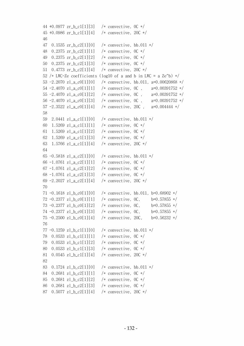
- 132 -
44 +0.0977 zr_b_c1[1][3] /* convective, 0C */
45 +0.0986 zr_b_c1[1][4] /* convective, 20C */
46
47 0.1535 zr_b_c2[1][0] /* convective, bb.011 */
48 0.2375 zr_b_c2[1][1] /* convective, 0C */
49 0.2375 zr_b_c2[1][2] /* convective, 0C */
50 0.2375 zr_b_c2[1][3] /* convective, 0C */
51 0.4773 zr_b_c2[1][4] /* convective, 20C */
52 /* LWC-Ze coefficients (log10 of a and b in LWC = a Ze^b) */
53 -2.2070 zl_a_c0[1][0] /* convective, bb.011, a=0.00620868 */
54 -2.4070 zl_a_c0[1][1] /* convective, 0C , a=0.00391752 */
55 -2.4070 zl_a_c0[1][2] /* convective, 0C , a=0.00391752 */
56 -2.4070 zl_a_c0[1][3] /* convective, 0C , a=0.00391752 */
57 -2.3522 zl_a_c0[1][4] /* convective, 20C , a=0.004444 */
58
59 2.0441 zl_a_c1[1][0] /* convective, bb.011 */
60 1.5269 zl_a_c1[1][1] /* convective, 0C */
61 1.5269 zl_a_c1[1][2] /* convective, 0C */
62 1.5269 zl_a_c1[1][3] /* convective, 0C */
63 1.5766 zl_a_c1[1][4] /* convective, 20C */
64
65 -0.5818 zl_a_c2[1][0] /* convective, bb.011 */
66 -1.0761 zl_a_c2[1][1] /* convective, 0C */
67 -1.0761 zl_a_c2[1][2] /* convective, 0C */
68 -1.0761 zl_a_c2[1][3] /* convective, 0C */
69 -2.2027 zl_a_c2[1][4] /* convective, 20C */
70
71 -0.1618 zl_b_c0[1][0] /* convective, bb.011, b=0.68902 */
72 -0.2377 zl_b_c0[1][1] /* convective, 0C, b=0.57855 */
73 -0.2377 zl_b_c0[1][2] /* convective, 0C, b=0.57855 */
74 -0.2377 zl_b_c0[1][3] /* convective, 0C, b=0.57855 */
75 -0.2500 zl_b_c0[1][4] /* convective, 20C, b=0.56232 */
76
77 -0.1259 zl_b_c1[1][0] /* convective, bb.011 */
78 0.0533 zl_b_c1[1][1] /* convective, 0C */
79 0.0533 zl_b_c1[1][2] /* convective, 0C */
80 0.0533 zl_b_c1[1][3] /* convective, 0C */
81 0.0545 zl_b_c1[1][4] /* convective, 20C */
82
83 0.1724 zl_b_c2[1][0] /* convective, bb.011 */
84 0.2681 zl_b_c2[1][1] /* convective, 0C */
85 0.2681 zl_b_c2[1][2] /* convective, 0C */
86 0.2681 zl_b_c2[1][3] /* convective, 0C */
87 0.5077 zl_b_c2[1][4] /* convective, 20C */
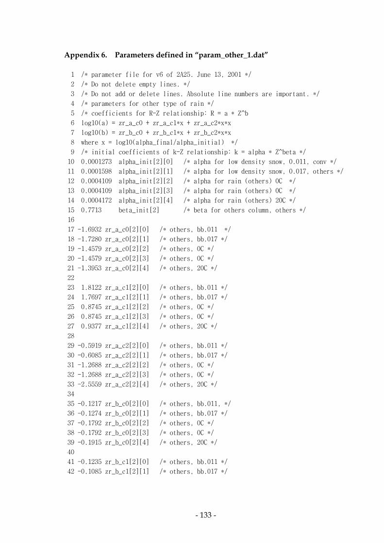
- 133 -
Appendix 6. Parameters defined in “param_other_1.dat” 1 /* parameter file for v6 of 2A25. June 13, 2001 */
2 /* Do not delete empty lines. */
3 /* Do not add or delete lines. Absolute line numbers are important. */
4 /* parameters for other type of rain */
5 /* coefficients for R-Z relationship: R = a * Z^b
6 log10(a) = zr_a_c0 + zr_a_c1*x + zr_a_c2*x*x
7 log10(b) = zr_b_c0 + zr_b_c1*x + zr_b_c2*x*x
8 where x = log10(alpha_final/alpha_initial) */
9 /* initial coefficients of k-Z relationship: k = alpha * Z^beta */
10 0.0001273 alpha_init[2][0] /* alpha for low density snow, 0.011, conv */
11 0.0001598 alpha_init[2][1] /* alpha for low density snow, 0.017, others */
12 0.0004109 alpha_init[2][2] /* alpha for rain (others) 0C */
13 0.0004109 alpha_init[2][3] /* alpha for rain (others) 0C */
14 0.0004172 alpha_init[2][4] /* alpha for rain (others) 20C */
15 0.7713 beta_init[2] /* beta for others column, others */
16
17 -1.6932 zr_a_c0[2][0] /* others, bb.011 */
18 -1.7280 zr_a_c0[2][1] /* others, bb.017 */
19 -1.4579 zr_a_c0[2][2] /* others, 0C */
20 -1.4579 zr_a_c0[2][3] /* others, 0C */
21 -1.3953 zr_a_c0[2][4] /* others, 20C */
22
23 1.8122 zr_a_c1[2][0] /* others, bb.011 */
24 1.7697 zr_a_c1[2][1] /* others, bb.017 */
25 0.8745 zr_a_c1[2][2] /* others, 0C */
26 0.8745 zr_a_c1[2][3] /* others, 0C */
27 0.9377 zr_a_c1[2][4] /* others, 20C */
28
29 -0.5919 zr_a_c2[2][0] /* others, bb.011 */
30 -0.6085 zr_a_c2[2][1] /* others, bb.017 */
31 -1.2688 zr_a_c2[2][2] /* others, 0C */
32 -1.2688 zr_a_c2[2][3] /* others, 0C */
33 -2.5559 zr_a_c2[2][4] /* others, 20C */
34
35 -0.1217 zr_b_c0[2][0] /* others, bb.011, */
36 -0.1274 zr_b_c0[2][1] /* others, bb.017 */
37 -0.1792 zr_b_c0[2][2] /* others, 0C */
38 -0.1792 zr_b_c0[2][3] /* others, 0C */
39 -0.1915 zr_b_c0[2][4] /* others, 20C */
40
41 -0.1235 zr_b_c1[2][0] /* others, bb.011 */
42 -0.1085 zr_b_c1[2][1] /* others, bb.017 */

- 134 -
43 +0.0977 zr_b_c1[2][2] /* others, 0C */
44 +0.0977 zr_b_c1[2][3] /* others, 0C */
45 +0.0986 zr_b_c1[2][4] /* others, 20C */
46
47 0.1535 zr_b_c2[2][0] /* others, bb.011 */
48 0.1520 zr_b_c2[2][1] /* others, bb.017 */
49 0.2375 zr_b_c2[2][2] /* others, 0C */
50 0.2375 zr_b_c2[2][3] /* others, 0C */
51 0.4773 zr_b_c2[2][4] /* others, 20C */
52 /* LWC-Ze coefficients (log10 of a and b in LWC = a Ze^b) */
53 -2.2070 zl_a_c0[2][0] /* others, bb.011, a=0.00620868 */
54 -2.2699 zl_a_c0[2][1] /* others, bb.02, a=0.00537114 */
55 -2.4070 zl_a_c0[2][2] /* others, 0C , a=0.00391752 */
56 -2.4070 zl_a_c0[2][3] /* others, 0C , a=0.00391752 */
57 -2.3522 zl_a_c0[2][4] /* others, 20C , a=0.004444 */
58
59 2.0441 zl_a_c1[2][0] /* others, bb.011 */
60 1.9998 zl_a_c1[2][1] /* others, bb.02 */
61 1.5269 zl_a_c1[2][2] /* others, 0C */
62 1.5269 zl_a_c1[2][3] /* others, 0C */
63 1.5766 zl_a_c1[2][4] /* others, 20C */
64
65 -0.5818 zl_a_c2[2][0] /* others, bb.011 */
66 -0.5713 zl_a_c2[2][1] /* others, bb.02 */
67 -1.0761 zl_a_c2[2][2] /* others, 0C */
68 -1.0761 zl_a_c2[2][3] /* others, 0C */
69 -2.2027 zl_a_c2[2][4] /* others, 20C */
70
71 -0.1618 zl_b_c0[2][0] /* others, bb.011, b=0.68902 */
72 -0.1675 zl_b_c0[2][1] /* others, bb.02, b=0.68004 */
73 -0.2377 zl_b_c0[2][2] /* others, 0C, b=0.57855 */
74 -0.2377 zl_b_c0[2][3] /* others, 0C, b=0.57855 */
75 -0.2500 zl_b_c0[2][4] /* others, 20C, b=0.56232 */
76
77 -0.1259 zl_b_c1[2][0] /* others, bb.011 */
78 -0.1099 zl_b_c1[2][1] /* others, bb.02 */
79 +0.0533 zl_b_c1[2][2] /* others, 0C */
80 +0.0533 zl_b_c1[2][3] /* others, 0C */
81 +0.0545 zl_b_c1[2][4] /* others, 20C */
82
83 0.1724 zl_b_c2[2][0] /* others, bb .011 */
84 0.1662 zl_b_c2[2][1] /* others, bb .017 */
85 0.2681 zl_b_c2[2][2] /* others, 0C */
86 0.2681 zl_b_c2[2][3] /* others, 0C */
87 0.5077 zl_b_c2[2][4] /* others, 20C */

- 135 -
3. Level 3
3-1. 3A-25: Space Time Statistics of Level 2 PR Products
1. Objective of the algorithm
The objective of the algorithm is to calculate various statistics over a month from the level 2 PR output products. Four types of statistics are calculated:
1. Probabilities of occurrence (count values) 2. Means and standard deviations 3. Histograms 4. Correlation coefficients
In all cases, the statistics are conditioned on the presence of rain or some other quantity such as the presence of stratiform rain or the presence of a bright-band. For example, to compute the unconditioned mean rain rate, the conditional mean must be multiplied by the probability of rain which, in turn is calculated from the ratio of rain counts to the total number of observations in the box of interest. Details of the procedure are given in section 8. The standard space scale is a 5×5-degree latitude×longitude cell. A subset of the products, however, is also produced over 0.5×0.5-degree cells. The types of statistics computed include: At 5×5-degree×1-month cells:
• Means, standard deviations, and count values (“pixel counts”) • Histograms • Correlation coefficients • RZ coefficients, a and b, R = aZb
At 0.5×0.5-degree×1-month cells:
• Means, standard deviations, and count values • RZ coefficients, a and b, R = aZb
The 5×5-degree statistics are stored in arrays dimensioned (16,72,*), with a product name ending with “1” (generally). There are 16 latitude cells, 72 longitude cells, and possibly other dimensions, as noted, for height, rain type, etc. Histograms are dimensioned (16,72,30,*) with 30 categories. The 0.5×0.5-degree statistics are dimensioned (148,720,*), and have a product name ending with “2”. There are 148 latitude cells and 720 longitude cells.

- 136 -
2. Output Variables
2.1 Variable naming convention Variable names consist of a word or several words strung together describing the geophysical quantity, and ending with an abbreviation designating the statistic type. For example, the 5×5-degree mean of stratiform rain rate is stratRainMean1. The statistic type designations are Mean1 5×5-degree means Dev1 5×5-degree standard deviations Pix1 5×5-degree pixel counts H histograms CCoef correlation coefficients rz..A1 RZ-relation a-coefficient, 5×5 degrees; “rz” is a prefix rz..B1 RZ-relation b-coefficient, 5×5 degrees Mean2 0.5×0.5-degree means Dev2 0.5×0.5-degree standard deviations Pix2 0.5×0.5-degree pixel counts rz..A2 RZ-relation a-coefficient, 0.5×0.5 degrees rz..B2 RZ-relation b-coefficient, 0.5×0.5 degrees For example, a typical set of statistics, for rain rate is: rainMean1(16,72,6) 1-month mean, 5×5-degree cells rainDev1(16,72,6) Standard deviation, 5×5-degree cells rainPix1(16,72,6) Count, 5×5-degree cells rainH(16,72,30,6) Histogram, 5×5-degree cells rainMean2(148,720,4) 1-month mean, 0.5×0.5-degree cells rainDev2(148,720,4) Standard deviation, 0.5×0.5-degree cells rainPix2(148,720,4) Count, 0.5×0.5-degree cells

- 137 -
2.2 Variable Definitions
Number of observations (rain and no-rain) ttlPix1(16,72) integer ttlPix2(148,720) integer Rain Rate Statistics Rain rates in mm/h CAPPIs Conditioned on the detection of rain (‘rain-certain’ flag), computed at 5 heights + path-averaged. The heights are 2, 4, 6, 10, 15-km and full-path. High-resolution statistics are computed at 3 heights + path-averaged, 2, 4, 6-km and full path. All rain types rainMean1(16,72,6) real rainDev1(16,72,6) real rainPix1(16,72,6) integer rainH(16,72,30,6) integer*2 rainMean2(148,720,4) real rainDev2(148,720,4) real rainPix2(148,720,4) integer Convective rain convRainMean1(16,72,6) real convRainDev1(16,72,6) real convRainPix1(16,72,6) integer convRainH(16,72,30,6) integer*2 convRainMean2(148,720,4) real convRainDev2(148,720,4) real convRainPix2(148,720,4) integer Stratiform rain stratRainMean1(16,72,6) real stratRainDev1(16,72,6) real stratRainPix1(16,72,6) integer stratRainH(16,72,30,6) integer*2 stratRainMean2(148,720,4 real stratRainDev2(148,720,4) real stratRainPix2(148,720,4) integer

- 138 -
Near-surface rain Conditioned on the detection of rain (‘rain certain’), computed at the nearest range bin judged free of ground clutter. The height in the input data varies with angle bin. All rain types surfRainMean1(16,72) real surfRainDev1(16,72) real surfRainPix1(16,72) integer surfRainH(16,72,30) integer*2 surfRainMean2(148,720) real surfRainDev2(148,720) real surfRainPix2(148,720) integer Convective rain surfRainConvMean1(16,72) real surfRainConvDev1(16,72) real surfRainConvPix1(16,72) integer surfRainConvH(16,72,30) integer*2 surfRainConvMean2(148,720) real surfRainConvDev2(148,720) real surfRainConvPix2(148,720) integer Stratiform rain surfRainStratMean1(16,72) real surfRainStratDev1(16,72) real surfRainStratPix1(16,72) integer surfRainStratH(16,72,30) integer*2 surfRainStratMean2(148,720) real surfRainStratDev2(148,720) real surfRainStratPix2(148,720) integer Estimated surface rain Conditioned on the detection of rain (“rain certain”), surface rain rate, estimated in 2A-25. All rain types e_surfRainMean1(16,72) real e_surfRainDev1(16,72) real e_surfRainPix1(16,72) integer e_surfRainH(16,72,30) integer*2 e_surfRainMean2(148,720) real e_surfRainDev2(148,720) real e_surfRainPix2(148,720) integer

- 139 -
Convective rain e_surfRainConvMean1(16,72) real e_surfRainConvDev1(16,72) real e_surfRainConvPix1(16,72) integer e_surfRainConvH(16,72,30) integer*2 e_surfRainConvMean2(148,720) real e_surfRainConvDev2(148,720) real e_surfRainConvPix2(148,720) integer Stratiform rain e_surfRainStratMean1(16,72) real e_surfRainStratDev1(16,72) real e_surfRainStratPix1(16,72) integer e_surfRainStratH(16,72,30) integer*2 e_surfRainStratMean2(148,720) real e_surfRainStratDev2(148,720) real e_surfRainStratPix2(148,720) integer Shallow/Shallow-isolated rain Near-surface rain, computed when rain is flagged “Shallow” or “Shallow-isolated”. The categories Shallow and Shallow-isolated are mutually exclusive. shallowRainMean1(16,72) real shallowRainDev1(16,72) real shallowRainPix1(16,72) integer shallowRainH(16,72,30) integer*2 shallowRainMean2(148,720) real shallowRainDev2(148,720) real shallowRainPix2(148,720) integer shallowIsoRainMean1(16,72) real shallowIsoRainDev1(16,72) real shallowIsoRainPix1(16,72) integer shallowIsoRainH(16,72,30) integer*2 shallowIsoRainMean2(148,720) real shallowIsoRainDev2(148,720) real shallowIsoRainPix2(148,720) integer

- 140 -
Measured reflectivity factors, Zm dBZ, Z in mm6/m3 CAPPIs Computed at the same heights and conditions as rain CAPPIs. The count values are the corresponding rain-rate pixel counts. 0.5×0.5-degree standard deviations are not computed. All rain types zmMean1(16,72,6) real zmDev1(16,72,6) real zmH(16,72,30,6) integer*2 zmMean2(148,720,4) real Convective rain convZmMean1(16,72,6) real convZmDev1(16,72,6) real convZmH(16,72,30,6) integer*2 convZmMean2(148,720,4) real Stratiform rain stratZmMean1(16,72,6) real stratZmDev1(16,72,6) real stratZmH(16,72,30,6) integer*2 stratZmMean2(148,720,4) real Attenuation-corrected estimate of reflectivity factor, Zt (“Z-true”) dBZ, Z in mm6/m3 CAPPIs Computed at the same heights and conditions as rain CAPPIs. The count values are the corresponding rain-rate pixel counts. 0.5×0.5-degree standard deviations are not computed. All rain types ztMean1(16,72,6) real ztDev1(16,72,6) real ztH(16,72,30,6) integer*2 ztMean2(148,720,4) real Convective rain convZtMean1(16,72,6) real convZtDev1(16,72,6) real convZtH(16,72,30,6) integer*2 convZtMean2(148,720,4) real

- 141 -
Stratiform rain stratZtMean1(16,72,6) real stratZtDev1(16,72,6) real stratZtH(16,72,30,6) integer*2 stratZtMean2(148,720,4) real Epsilon-0 and epsilon Epsilon_0 is defined as the multiplicative factor of α (in the k=αZβ relation) such that the path attenuation from Hitschfeld-Bordan estimate is equal to that from the surface reference technique (SRT). For small values of attenuation it is approximately equal to the ratio of the path attenuation from the SRT to that of the Hitschfeld-Bordan path attenuation. It is computed only when the path attenuation from 2A-21 is judged to be reliable or marginally reliable (see 2A-21) and when bit 8 of the method flag from 2A-25 is set to one. Epsilon is the multiplicative factor of α for the hybrid method of 2A-25. For small values of attenuation it is approximately equal to the ratio of the path attenuation from 2A-25 to that of the Hitschfeld-Bordan path attenuation. The epsilon values are stored only under the conditions for which the epsilon_0 data are stored. The number of counts for epsilon and epsilon_0 should be the same. Specifically, epsilon0StratPix1 = epsilonStratPix1 epsilon0ConvPix1 = epsilonConvPix1 epsilon0StratPix2 = epsilonStratPix2 epsilon0ConvPix2 = epsilonConvPix2 Epsilon is the ratio of the path attenuation from 2A-25 to that of the Hitschfeld-Bordan path attenuation (see 2a25). epsilon0ConvMean1(16,72) real epsilon0ConvDev1(16,72) real epsilon0ConvPix1(16,72) integer epsilon0ConvH(16,72,30) integer*2 epsilon0ConvMean2(148,720) real epsilon0ConvDev2(148,720) real epsilon0ConvPix2(148,720) integer epsilon0StratMean1(16,72) real epsilon0StratDev1(16,72) real epsilon0StratPix1(16,72) integer epsilon0StratH(16,72,30) integer*2 epsilon0StratMean2(148,720) real epsilon0StratDev2(148,720) real epsilon0StratPix2(148,720) integer
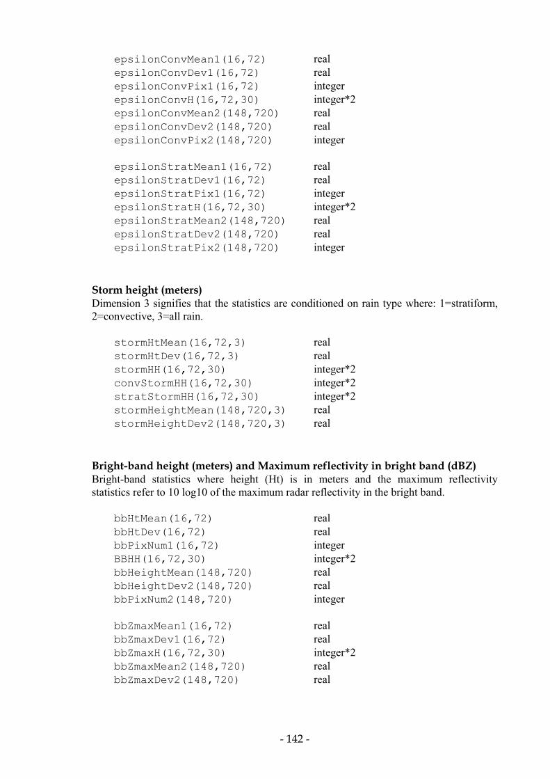
- 142 -
epsilonConvMean1(16,72) real epsilonConvDev1(16,72) real epsilonConvPix1(16,72) integer epsilonConvH(16,72,30) integer*2 epsilonConvMean2(148,720) real epsilonConvDev2(148,720) real epsilonConvPix2(148,720) integer epsilonStratMean1(16,72) real epsilonStratDev1(16,72) real epsilonStratPix1(16,72) integer epsilonStratH(16,72,30) integer*2 epsilonStratMean2(148,720) real epsilonStratDev2(148,720) real epsilonStratPix2(148,720) integer Storm height (meters) Dimension 3 signifies that the statistics are conditioned on rain type where: 1=stratiform, 2=convective, 3=all rain. stormHtMean(16,72,3) real stormHtDev(16,72,3) real stormHH(16,72,30) integer*2 convStormHH(16,72,30) integer*2 stratStormHH(16,72,30) integer*2 stormHeightMean(148,720,3) real stormHeightDev2(148,720,3) real Bright-band height (meters) and Maximum reflectivity in bright band (dBZ) Bright-band statistics where height (Ht) is in meters and the maximum reflectivity statistics refer to 10 log10 of the maximum radar reflectivity in the bright band. bbHtMean(16,72) real bbHtDev(16,72) real bbPixNum1(16,72) integer BBHH(16,72,30) integer*2 bbHeightMean(148,720) real bbHeightDev2(148,720) real bbPixNum2(148,720) integer bbZmaxMean1(16,72) real bbZmaxDev1(16,72) real bbZmaxH(16,72,30) integer*2 bbZmaxMean2(148,720) real bbZmaxDev2(148,720) real
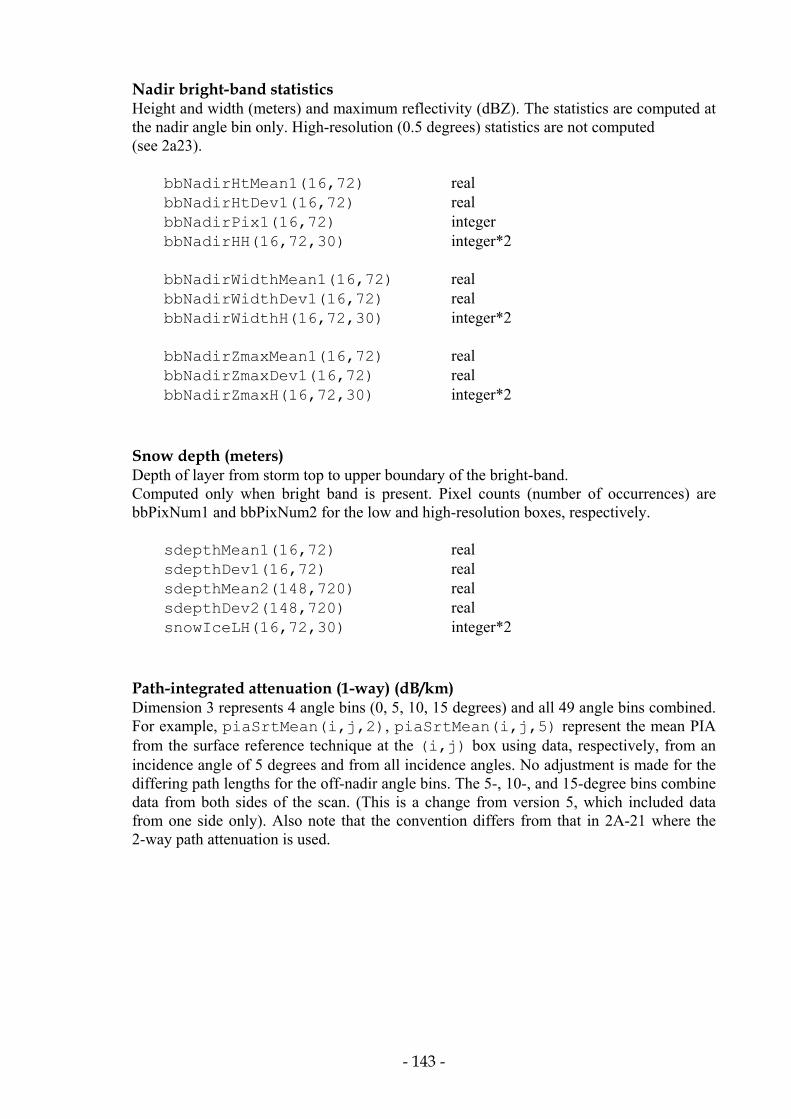
- 143 -
Nadir bright-band statistics Height and width (meters) and maximum reflectivity (dBZ). The statistics are computed at the nadir angle bin only. High-resolution (0.5 degrees) statistics are not computed (see 2a23). bbNadirHtMean1(16,72) real bbNadirHtDev1(16,72) real bbNadirPix1(16,72) integer bbNadirHH(16,72,30) integer*2 bbNadirWidthMean1(16,72) real bbNadirWidthDev1(16,72) real bbNadirWidthH(16,72,30) integer*2 bbNadirZmaxMean1(16,72) real bbNadirZmaxDev1(16,72) real bbNadirZmaxH(16,72,30) integer*2 Snow depth (meters) Depth of layer from storm top to upper boundary of the bright-band. Computed only when bright band is present. Pixel counts (number of occurrences) are bbPixNum1 and bbPixNum2 for the low and high-resolution boxes, respectively. sdepthMean1(16,72) real sdepthDev1(16,72) real sdepthMean2(148,720) real sdepthDev2(148,720) real snowIceLH(16,72,30) integer*2 Path-integrated attenuation (1-way) (dB/km) Dimension 3 represents 4 angle bins (0, 5, 10, 15 degrees) and all 49 angle bins combined. For example, piaSrtMean(i,j,2), piaSrtMean(i,j,5) represent the mean PIA from the surface reference technique at the (i,j) box using data, respectively, from an incidence angle of 5 degrees and from all incidence angles. No adjustment is made for the differing path lengths for the off-nadir angle bins. The 5-, 10-, and 15-degree bins combine data from both sides of the scan. (This is a change from version 5, which included data from one side only). Also note that the convention differs from that in 2A-21 where the 2-way path attenuation is used.

- 144 -
Notation: ‘Srt’ denotes the path attenuation determined from the surface reference technique in 2A-21. Data are added to the computation only when the path attenuation is judged to be reliable or marginally reliable. ‘Hb’ denotes the Hitschfeld-Bordan path attenuation from 2A-25. In some cases, the estimate diverges so the estimates are not included in the statistics ‘2a25’ denotes the final path attenuation estimate from 2a25 ‘0’ denotes the zeroth-order estimate of path attenuation as determined from the integral of αZm
β integrated from the storm top to the lowest range gate. α and β are estimated in 2A-25 piaSrtMean(16,72,5) real piaSrtDev(16,72,5) real piaSrtPix(16,72,5) real piaSrtH(16,72,30,5) integer*2 piaHbMean(16,72,5) real piaHbDev(16,72,5) real piaHbPix(16,72,5) real piaHbH(16,72,30,5) integer*2 pia0Mean(16,72,5) real pia0Dev(16,72,5) real pia0Pix(16,72,5) real pia0H(16,72,30,5) integer*2 pia2a25Mean(16,72,5) real pia2a25Dev(16,72,5) real pia2a25Pix(16,72,5) real pia2a25H(16,72,30,5) integer*2 Subset PIA statistics are the same as the above statistics, except that the input data are filtered the same way as the epsilon statistics. piaSrtssMean(16,72,5) real piaSrsstDev(16,72,5) real piaSrtssPix(16,72,5) real piaSrtssH(16,72,30,5) integer*2 piaHbssMean(16,72,5) real piaHbssDev(16,72,5) real piaHbssPix(16,72,5) real piaHbssH(16,72,30,5) integer*2

- 145 -
pia0ssMean(16,72,5) real pia0ssDev(16,72,5) real pia0ssPix(16,72,5) real pia0ssH(16,72,30,5) integer*2 pia2a25ssMean(16,72,5) real pia2a25ssDev(16,72,5) real pia2a25ssPix(16,72,5) real pia2a25ssH(16,72,30,5) integer*2 Xi (unitless) Xi is the normalized standard deviation of zeta (see 2A-25), zeta_sd/zeta_mn. Xi is no longer a product in 2A-25, but zeta_sd and zeta_mn are available. In version 6, xi is now computed in 3A-25. Xi is set to zero when zeta_mn is less than 0.01. xiMean(16,72) real xiDev(16,72) real xiH(16,72,30) integer*2 Non-uniform beam filling correction factor (unitless, see 2a25) nubfCorFacMean(16,72) real nubfCorFacDev(16,72) real nubfH(16,72,30) integer*2 RZ-relation coefficients, a and b, R = aZb Computed near-surface (last array dimension = 1) and at 2-km (last dimension = 2). At each lat-lon cell, a logR-logZ fit is computed for all pairs of points (logR, logZ) that are estimated within the box (at either near-surface or 2 km) for the month. Note that R is rain rate (mm/h) and Z is the attenuation-corrected reflectivity. If the a coefficient exceeds 10, the fit is assumed to have failed, and both a and b are set to -999.0. All rain types rzA1(16,72,2) real rzB1(16,72,2) real rzPix1(16,72,2) integer rzA2(148,720,2) real rzB2(148,720,2) real rzPix2(148,720,2) integer
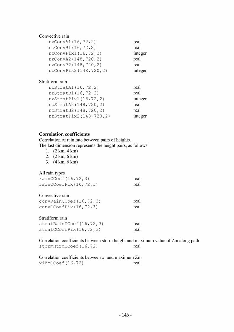
- 146 -
Convective rain rzConvA1(16,72,2) real rzConvB1(16,72,2) real rzConvPix1(16,72,2) integer rzConvA2(148,720,2) real rzConvB2(148,720,2) real rzConvPix2(148,720,2) integer Stratiform rain rzStratA1(16,72,2) real rzStratB1(16,72,2) real rzStratPix1(16,72,2) integer rzStratA2(148,720,2) real rzStratB2(148,720,2) real rzStratPix2(148,720,2) integer Correlation coefficients Correlation of rain rate between pairs of heights. The last dimension represents the height pairs, as follows:
1. (2 km, 4 km) 2. (2 km, 6 km) 3. (4 km, 6 km)
All rain types rainCCoef(16,72,3) real rainCCoefPix(16,72,3) real Convective rain convRainCCoef(16,72,3) real convCCoefPix(16,72,3) real Stratiform rain stratRainCCoef(16,72,3) real stratCCoefPix(16,72,3) real Correlation coefficients between storm height and maximum value of Zm along path stormHtZmCCoef(16,72) real Correlation coefficients between xi and maximum Zm xiZmCCoef(16,72) real

- 147 -
PIA correlation coefficients These are the correlations between various PIA estimates. Dimension 3 represents 4 angle bins (0, 5, 10, 15 degrees) and all 49 angle bins combined. The last dimension represents the various pairs amongst four PIA estimates, as follows:
1. [SRT,HB] 2. [SRT,0th-order] 3. [HB,0th-order] 4. [2a25,SRT] 5. [2a25,HB] 6. [2a25,0th-order]
piaCCoef(16,72,5,6) real piaCCoefPix(16,72,5) real ttlAnglePix1(16,72,4) integer*2 rainAnglePix1(16,72,4) integer*2

- 148 -
2.3 Definition of Bins for Histograms For radar reflectivity factor histograms: ztH, convZtH, stratZtH zmH, convZmH, stratZmH bbZmaxH, bbNadirZmaxH, the 31 bin boundaries are: 0.01 12.0 14.0 16.0 18.0 20.0 22.0 24.0 26.0 28.0 30.0 32.0 34.0 36.0 38.0 40.0 42.0 44.0 46.0 48.0 50.0 52.0 54.0 56.0 58.0 60.0 62.0 64.0 66.0 68.0 70.0 For all rain rate histograms: rainH, stratRainH, convRainH, surfRainH, the 31 bin boundaries are (mm/h): 0.01 0.2050482 0.2734362 0.3646330 0.4862459 0.6484194 0.8646811 1.153071 1.537645 2.050482 2.734362 3.646330 4.862459 6.484194 8.646811 11.53071 15.37645 20.50482 27.34362 36.46331 48.62460 64.84194 86.46812 115.3071 153.7645 205.0482 273.4362 364.6331 486.2460 648.4194 864.6812 For bright band height histogram, HHBB, the 31 bin boundaries [km] are: 0.01 0.25 0.50 0.75 1.00 1.25 1.50 1.75 2.00 2.25 2.50 2.75 3.00 3.25 3.50 3.75 4.00 4.25 4.50 4.75 5.00 5.25 5.50 5.75 6.00 6.25 6.50 6.75 7.00 7.50 20.00 For storm height histograms, stormHH, stratStormHH, convStormHH, (in km), the 31 bin boundaries [km] are: 0.01 0.5 1.0 1.5 2.0 2.5 3.0 3.5 4.0 4.5 5.0 5.5 6.0 6.5 7.0 7.5 8.0 8.5 9.0 9.5 10.0 10.5 11.0 11.5 12.0 12.5 13.0 14.0 15.0 16.0 20.0 For distance from storm top to bright-band height histogram, snowIceLH, bbNadirWidthH, the 31 bin boundaries [m] are: 0.0 125.0 250.0 375.0 500.0 625.0 750.0 875.0 1000.0 1125.0 1250.0 1375.0 1500.0 1625.0 1750.0 1875.0 2000.0 2125.0 2250.0 2375.0 2500.0 2625.0 2750.0 2875.0 3000.0 3125.0 3250.0 3375.0 3500.0 3625.0 3750.0

- 149 -
For the path-averaged attenuation estimate histograms, piaSrtH, piaHbH, pia0H, and pia2a25H, the 31 bin boundaries [dB] are: 0.01 0.1 0.2 0.3 0.4 0.5 0.6 0.8 1.0 1.2 1.4 1.6 1.8 2.0 2.5 3.0 3.5 4.0 4.5 5.0 5.5 6.0 7.0 8.0 9.0 10.0 15.0 20.0 25.0 30.0 100. For non-uniform beamfilling factor histogram, nubfH, the 31 bin boundaries [dimensionless] are: 1.00 1.05 1.10 1.15 1.20 1.25 1.30 1.35 1.40 1.45 1.50 1.55 1.60 1.65 1.70 1.75 1.80 1.85 1.90 1.95 2.00 2.10 2.20 2.30 2.40 2.50 2.60 2.70 2.80 2.90 3.00 For xi (=standard deviation of zeta/mean of zeta) histogram, xiH, the 31 bin boundaries [dimensionless] are: 0.0 0.2 0.4 0.6 0.8 1.0 1.2 1.4 1.6 1.8 2.0 2.2 2.4 2.6 2.8 3.0 3.2 3.4 3.6 3.8 4.0 4.2 4.4 4.6 4.8 5.0 10.0 20.0 30.0 50.0 10000. For the parameters epsilon and epsilon0 (see 2a25) the 31 bin boundaries are: 0.0 0.1 0.2 0.3 0.4 0.5 0.6 0.7 0.8 0.9 1.0 1.1 1.2 1.3 1.4 1.5 1.6 1.7 1.8 1.9 2.0 2.1 2.2 2.3 2.4 2.5 2.6 2.7 2.8 2.9 3.0 2.4 Other Input Parameters: CAPPI heights relative to the ellipsoid: 2, 4, 6, 10, 15 km. Angle bins at which the statistics of the various PIA estimates are to be evaluated: 5, 12, 18, 25, 32, 38, 45, which correspond approximately to angles of 0, 5, 10, and 15 degrees incidence (port and starboard).
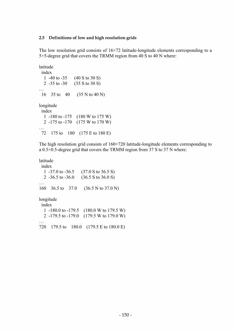
- 150 -
2.5 Definitions of low and high resolution grids The low resolution grid consists of 16×72 latitude-longitude elements corresponding to a 5×5-degree grid that covers the TRMM region from 40 S to 40 N where: latitude index 1 -40 to -35 (40 S to 30 S) 2 -35 to -30 (35 S to 30 S) … 16 35 to 40 (35 N to 40 N) longitude index 1 -180 to -175 (180 W to 175 W) 2 -175 to -170 (175 W to 170 W) … 72 175 to 180 (175 E to 180 E) The high resolution grid consists of 160×720 latitude-longitude elements corresponding to a 0.5×0.5-degree grid that covers the TRMM region from 37 S to 37 N where: latitude index 1 -37.0 to -36.5 (37.0 S to 36.5 S) 2 -36.5 to -36.0 (36.5 S to 36.0 S) … 160 36.5 to 37.0 (36.5 N to 37.0 N) longitude index 1 -180.0 to -179.5 (180.0 W to 179.5 W) 2 -179.5 to -179.0 (179.5 W to 179.0 W) … 720 179.5 to 180.0 (179.5 E to 180.0 E)

- 151 -
3. Processing Procedure:
The basic steps in the procedure are: i. Read in data (scan by scan) from 2A-21, 2A-23, 2A-25 and 1C-21. ii. Adjust the numbering conventions so that Zm, Zt and R are aligned properly; this is
done by using the anchor point of binEllipsoid in 1C-21 and the corresponding bin ellipsoid of 2A-25 which, by convention, is the 80th element of Zt.
iii. Find the coarse and fine resolution boxes to which each of the 49 observations belongs.
Note that a single scan is composed of 49 observations each at a different incidence angle. (coarse resolution boxes are 5×5-degree cells) (fine resolution boxes are 0.5×0.5-degree cells)
iv. Resample Zm, Zt and R from the range direction onto the vertical. v. Update the various statistics. vi. If a month transition occurs within the granule, write the HDF output file and
reinitialize the intermediate files. 4. Comments and Issues: i. In version 6, the rain statistics are computed only when the ‘rain-certain’ flag is set in
1C-21. The ‘rain-possible’ flag is treated the same as a ‘no-rain’ flag. Products defined in version 4 (which contained the term ‘All’ in the product name) and which included ‘rain-certain’ and ‘rain-possible’ data, have been deleted from the list of version 6 products.
ii. It is assumed in the program that the verification file does not exist; if it is already
exists an error will occur. iii. There are 2 definitions of zeta and nubf (from 2A-25). In both cases the original
definitions of these quantities are used; i.e., the first element of the array. iv. The height levels are being defined relative to the ellipsoid and not the local surface.
This may cause difficulties in the interpretation of the statistics over some land areas at the lower height levels because the level can be below the local surface. In these cases, the rain rate is always set to some flag value and is not counted in the statistics. On the other hand, ttlPix1 (or ttlPix2), the total number of valid observations at the low (high) resolution averaging box, will be incremented so that the observations ‘below the surface’ will be counted as ‘no-rain’ events. This will introduce a negative bias into the mean rain rate at the (lat,long) box in question.

- 152 -
v. Missing data scans are being checked by monitoring the scanStatus flags in 1C-21.
If this indicates a missing scan, no processing is done for that scan. Checks for individual missing variables are not being done explicitly, however.
vi. There are several subtle, interrelated issues regarding the definitions of rain and
no-rain and how these definitions affect the statistics. For most of the output products from level 2, numbers that represent a physical quantity (non-flagged values) are being output only if the minEchoFlag variable in 1C-21 is set to ‘rain-certain’. However, an important category of products (Zt and rain rate from 2A-25 and Zm from 1C-21) is being output under rain-possible conditions. With the exception noted above only those products for which rain detection is classified as ‘certain’ are included in the statistics (that is, the statistics conditioned on rain being present). Although some rain events will be missed, the advantage of this selection is that the set of products should be self-consistent. The above was valid for version 4. In versions 5 and 6 the rain-possible flag is always treated as a no-rain occurrence (see comment i.).
vii. The quantity ‘minEchoFlag’ (from 1B-21 and 1C-21) provides information on the
presence/absence of rain along each of the 49 angle bins that comprise the cross-track scan. To test whether rain is present at a particular range bin or height above the ellipsoid, a threshold value must be used. Presently, this threshold is dBZt > 0.01 dB so that if minEchoFlag indicates the certainty of rain along the beam and if dBZt > 0.01 dB at a particular range bin or height level, then the data (e.g., rain rate, dBZm, dBZt, etc) are used in the calculation of the statistics (mean and standard deviation). A difficulty arises in defining the histograms for the rain rates. The lowest histogram bin for dBZt and dBZm is taken from 0.01 dB to 12 dB; the subsequent bins are taken equal to 2 dB so that the bin boundaries are 14 dB, 16 dB,…, 70 dB. Since the Z-R relationship that is used in 2A-25 can change depending on the storm type and vertical structure, and because the histogram bins must be fixed, the bins for the quantity 10 log R (where R is the rain rate in mm/h) are determined from the nominal relationship Z = 200R1.6 or in dB: dBR = 0.625 dBZ - 14.38 . For example, the dBZ histogram bin from 12 dB to 14 dB corresponds to the rain rate histogram bin from -6.88 dB to -5.63 dB. The lowest dBR value (the lower boundary of the first bin) is 0.625×0.01-14.38 = -14.32 dB. It is possible, however, for dBR to be less than this because the actual Z-R relationship used in 2A-25 differs from the nominal relationship. In order to count all non-zero rain rates (under ‘rain-certain’ conditions), the lower boundary of the first dBR histogram bin is set to -20 dB rather than -14.32 dB. The reason for doing this is to ensure that the number of data points that are categorized in the rain rate histogram are equal to the number of data points used in the calculation of the mean and standard deviation of this quantity.

- 153 -
viii. There are 4 types of rain rates that are defined in 3a-25.
The first is a ‘near-surface’ rain rate that is obtained from the range bin closest to the surface that is not corrupted by the surface clutter. In version 4, two sets of products were being computed from these data: the first set of statistics used only those rain rate for which rain is classified as ‘certain’; the second set used those rain rates for which rain is classified either as ‘possible’ or ‘certain’. For version 5, the determination was made to eliminate products using the ‘rain-possible’ flag (see comment i). The second type of rain rate is the path-averaged rain rate calculated by summing the values from the storm top (first gate where rain is detected) to the last gate (gate nearest to the surface uncontaminated by the surface clutter) and dividing by the number of gates in the interval. The third type of rain rate is that at a fixed height above the ellipsoid (2, 4, 6, 10 and 15 km). For an arbitrary incidence angle there will be several range gates that intersect the height: to estimate dBZm, dBZt and rain rate at that height, a gaussian weighting is done in dB space for the reflectivity factors and in linear space for the rain rates. This resampling lowers the minimum detectable threshold that, in turn, affects the histogram counts in the 2 lowest bins. In other words, the histogram counts at the lowest 2 bins will generally be larger for the height-profiled quantities than for the ‘near-surface’ or ‘path-averaged’ quantities. The fourth type, added in version 6, is an estimated surface rain rate. See 2a25 for a discussion.
ix. As noted in comment v., the rain rate statistics over mountainous regions at the height
levels of 2 and 4 km will tend to underestimate the actual values; for these cases, the near-surface rain rate statistics (under ‘rain-certain’ conditions) should be a more reliable indicator of the near-surface rain rate.
x. All of the statistics in 3a25 are conditioned on the existence of one or more variables.
To compute the unconditioned statistic, it is necessary to compute the probabilities of the events upon which the statistic is conditioned. For example, rainMean1(i,j,k) is the conditional mean rain rate in the box (i,j) at the kth height level. To convert this into an unconditional mean rain rate, Rm say, it is necessary first to compute the probability of rain at the appropriate latitude-longitude box and height:
Pr(i, j,k) =rainPix1(i, j,k)
ttlPix1(i, j)
Rm (i, j,k) = Pr (i, j,k) × rainMean1(i, j,k) To convert this to an accumulation (in mm) over a time period consisting of N hours, a multiplication of Rm by N would be used. For example, the accumulation in mm in a 30 day month N = 720.

- 154 -
Similarly, to compute the unconditional mean rain rate for stratiform rain, Rm
Strat, at (i,j,k):
PrStrat (i, j,k) =
stratRainPix1(i, j,k)ttlPix1(i, j)
RmStrat (i, j,k) = Pr
Strat (i, j,k) × stratRainMean1(i, j,k) Note also the following probabilities:
Pr bright - band( )=bbPixNum(i, j)
ttlPix1(i, j)
Pr stratiform rainrain( )=stratRainPix1(i, j,k)
rainPix1(i, j,k)
Pr convective rainrain( )=convRainPix1(i, j,k)
rainPix1(i, j,k)
Pr bright - bandrain( )=bbPixNum(i, j,k)rainPix1(i, j,k)
Note the difference among quantities of the following kind:
Pr stratiform rainrain( )=stratRainPix1(i, j,k)
rainPix1(i, j,k)
′ P r stratiform rainrain( )=stratRainPix1(i, j,k)
rainPix1(i, j,6)
′ ′ P r stratiform rainrain( )= stratRainPix1(i, j,6)rainPix1(i, j,6)
Pr'' corresponds to what is the most common definition of the probability of stratiform rain: given that rain is present, what is the probability that it is stratiform. Pr is the probability that, given rain is present at a particular height level (denoted by the index k), that the rain is stratiform. Pr' is the probability that, given rain is present somewhere along the beam, that rain is present at height level k and that the rain is stratiform.

- 155 -
5. Changed Variables in Version 6 5.1 New variables
bbNadirPix1
bbNadirHtMean1
bbNadirHtDev1
bbNadirHH
bbNadirWidthMean1
bbNadirWidthDev1
bbNadirWidthH
bbNadirZmaxMean1
bbNadirZmaxDev1
bbNadirZmaxH
e_surfRainPix1
e_surfRainMean1
e_surfRainDev1
e_surfRainH
e_surfRainPix2
e_surfRainMean2
e_surfRainDev2
e_surfRainConvPix1
e_surfRainConvMean1
e_surfRainConvDev1
e_surfRainConvH
e_surfRainConvPix2
e_surfRainConvMean2
e_surfRainConvDev2
e_surfRainStratPix1
e_surfRainStratMean1
e_surfRainStratDev1
e_surfRainStratPix2
e_surfRainStratMean2
e_surfRainStratDev2
e_surfRainStratH
epsilon0ConvPix1
epsilon0ConvMean1
epsilon0ConvDev1
epsilon0ConvH
epsilon0ConvPix2
epsilon0ConvMean2
epsilon0ConvDev2
epsilon0StratPix1
epsilon0StratMean1
epsilon0StratDev1
epsilon0StratH
epsilon0StratPix2
epsilon0StratMean2
epsilon0StratDev2
epsilonConvPix1
epsilonConvMean1
epsilonConvDev1
epsilonConvH
epsilonConvPix2
epsilonConvMean2
epsilonConvDev2
epsilonStratPix1
epsilonStratMean1
epsilonStratDev1
epsilonStratH
epsilonStratPix2
epsilonStratMean2
epsilonStratDev2
pia0Pix
pia2a25Pix
piaHbPix
piaSrtPix
piaCCoefPix
piaSrtssPix
piaSrtssMean
piaSrsstDev
piaSrtssH
piaHbssPix
piaHbssMean
piaHbssDev
piaHbssH
pia0ssPix
pia0ssMean
pia0ssDev
pia0ssH
pia2a25ssPix
pia2a25ssMean
pia2a25ssDev
pia2a25ssH
convCCoefPix
stratCCoefPix
rainCCoefPix
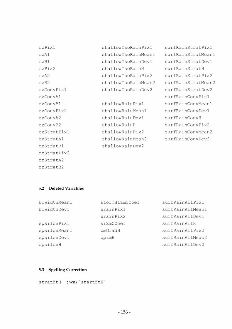
- 156 -
rzPix1
rzA1
rzB1
rzPix2
rzA2
rzB2
rzConvPix1
rzConvA1
rzConvB1
rzConvPix2
rzConvA2
rzConvB2
rzStratPix1
rzStratA1
rzStratB1
rzStratPix2
rzStratA2
rzStratB2
shallowIsoRainPix1
shallowIsoRainMean1
shallowIsoRainDev1
shallowIsoRainH
shallowIsoRainPix2
shallowIsoRainMean2
shallowIsoRainDev2
shallowRainPix1
shallowRainMean1
shallowRainDev1
shallowRainH
shallowRainPix2
shallowRainMean2
shallowRainDev2
surfRainStratPix1
surfRainStratMean1
surfRainStratDev1
surfRainStratH
surfRainStratPix2
surfRainStratMean2
surfRainStratDev2
surfRainConvPix1
surfRainConvMean1
surfRainConvDev1
surfRainConvH
surfRainConvPix2
surfRainConvMean2
surfRainConvDev2
5.2 Deleted Variables
bbwidthMean1
bbwidthDev1
epsilonPix1
epsilonMean1
epsilonDev1
epsilonH
stormHtZmCCoef
wrainPix1
wrainPix2
xiZmCCoef
zmGradH
zpzmH
surfRainAllPix1
surfRainAllMean1
surfRainAllDev1
surfRainAllH
surfRainAllPix2
surfRainAllMean2
surfRainAllDev2
5.3 Spelling Correction stratZtH ; was “startZtH”
- 157 -
3-2. 3A-26: Estimation of Space-Time Rain Rate Statistics Using a Multiple Thresholding Technique 1. Objective of the algorithm The primary objective of 3A-26 is to compute the rain rate statistics over 5-degree (latitude)×5-degree (longitude)×1-month space-time regions. The output products include the estimated values of the probability distribution function of the space-time rain rates at 4 “levels” (2 km, 4 km, 6 km and path-averaged) and the mean, standard deviation, and probability of rain derived from these distributions. Three different rain rate estimates are used for the high-resolution rain rate inputs to the algorithm: the standard Z-R (or 0th-order estimate having no attenuation correction), the Hitschfeld-Bordan (H-B), and the rain rates taken from 2a-25. (Fits based on the high-resolution inputs from the surface reference technique are output to the diagnostic file for evaluation). This algorithm is based on a statistical procedure. Although the radar team believes that a statistical method of this type should be implemented for TRMM, the method is relatively new and the testing has been carried out only on simulated data and on preliminary TRMM data. Caution on the use of the results is well warranted. 2. Description of the Method A general understanding of the method can be gained by noting that the amount of attenuation in the TRMM radar signal depends on the 2-way path attenuation down to the range gate of interest. This attenuation increases as the range gate is taken deeper into the storm (closer to the surface) and as the rain rate increases. Although some general features of the rain are used in 2a-25, the rain rate estimates are obtained at each instantaneous field of view (IFOV) of the instrument. The space-time statistics of these high-resolution estimates are done in 3a-25. Most users of the TRMM radar data will be interested in the output data from 3a-25 and not the data from 3a-26.

- 158 -
Algorithm 3a-26 serves as an alternative way of estimating the space-time rain statistics. The idea behind the method is that because of attenuation at high rain rates and low signal to noise ratios at light rain rates, there will usually exist an intermediate region over which the rain rate estimates are most accurate. Using only these estimates and an assumption as to the form of the probability distribution function (log-normal), the parameters of the distribution can be found by minimizing the rms difference between the hypothetical distribution and the values of the distribution obtained directly from the measurements. Once the distribution is estimated, the mean and standard deviation of the distribution can be calculated [Refs. 1-2, Ref. 6]. Useful by-products from the calculation of the probability distribution of rain rates are the fractional areas above (or below) particular rain rate thresholds. These data can be used as inputs to some of the area-time integral (ATI) methods that have been proposed [Refs. 3-5]. Although the data can be used to implement the ATI method, the method used in 3a-26 is itself not an ATI method. The behavior of the estimates depends strongly on the magnitude and type of threshold as well as the method that is used to determine the high-resolution rain rates. There are 3 methods that are used to determine the high-resolution rain rates: the Z-R (0th order without attenuation correction), the Hitschfeld-Bordan (H-B), and the hybrid method of 2a-25. A fourth method, based solely upon the surface reference method, is implemented in the code but the results are output only to a diagnostic file for evaluation. For the 3 estimates of rain rate (Z-R, HB and 2a-25), Q (or zeta as defined in 2a-25) is used as the threshold parameter. What this means is that if the threshold is set to a particular value, Q*, then if the measured value of Q is less than Q*, the corresponding rain rate is accepted - that is, it is used to update the distribution function of rain rates. On the other hand, if Q exceeds Q* the corresponding rain rate estimate is rejected - that is, it is not used to update the distribution function. As the threshold value, Q, is increased a larger percentage of the rain rates will be accepted. The converse holds so that as Q is decreased a smaller percentage of the rain rates will be used in estimating the distribution function. It should be noted that Q is a proxy for the attenuation and usually assumes a value between 0 and 1.

- 159 -
If the Z-R method (without attenuation correction) of estimating the high resolution rain rates is considered, the corresponding output files include the rain rate distribution function, zeroOrderpDf, and the mean, standard deviation, and probability of rain derived from the distribution, zeroOrderFit, for 6 different values of the Q threshold. The six values of Q are: 0.1, 0.2, 0.3, 0.5, 0.75 and 0.9999. Which set of values corresponding to which threshold should be used ? Simulations suggest that if the total number of rain points is on the order of 500 to 1000, the best accuracy is usually obtained by using a threshold value of 0.3. This corresponds to the 3rd array element so that the monthly mean rain rate (using the Z-R method) over the 5×5-degree box (lat, long) at height level, ih, is given by: mean = zeroOrderFit(lat, long, 1, ih, iq = 3)
The standard deviation and probability of rain are given by: std dev = zeroOrderFit(lat, long, 2, ih, iq = 3)
Pr (Rain) = zeroOrderFit(lat, long, 3, ih, iq = 3)
Simulations indicate that for a large number of rain points (N > 5000), the use of smaller threshold values (Q = 0.2) may lead to better estimates of the mean space-time rain rate. In the case of Q = 0.2 we have: Mean = zeroOrderFit(lat, long, 1, ih, iq = 2)
std dev = zeroOrderFit(lat, long, 2, ih, iq = 2)
Pr (Rain) = zeroOrderFit(lat, long, 3, ih, iq = 2)
A useful set for comparison is the choice: Q = 0.999 (array element 6). In this case nearly all of the Z-R rain rate estimates are accepted so that the method reduces to fitting almost all the Z-R derived rain rates to a lognormal distribution: Mean = zeroOrderFit(lat, long, 1, ih, iq = 6)
std dev = zeroOrderFit(lat, long, 2, ih, iq = 6)
Pr (Rain) = zeroOrderFit(lat, long, 3, ih, iq = 6)

- 160 -
The estimate of the mean as determined from the zeroOrderFit HDF output variable should be considered the primary output of the algorithm. Since Q = 0.3 is considered, nominally, as the optimum choice of threshold, the variable, rainMeanTH, has been defined to store these values. In particular: rainMeanTH(lat,long,ih) = zeroOrderFit(lat,long,ih,1,3)
The accuracy of the results at other Q thresholds and the statistics derived from the Hitschfeld-Bordan (hbFit) and rain rates from 2a-25 (fit2A25) will be evaluated as additional data from the TRMM radar become available. 3. Relationship of 3a-26 outputs to those of 3a-25 In comparing the statistics from 3a-25 and 3a-26 there are 2 differences between these data sets that should be kept in mind. The first is that the statistics produced from 3a-25 are conditioned either on the presence of rain or on the presence of a particular type of rain (stratiform or convective). For the 3a-26 products the means and standard deviations derived from the zeroOrderFit, hbFit and fit2A25 arrays are unconditioned - that is, the statistics include both rain and no-rain events. The second difference is that the set of heights for the 3a-26 products is a subset of the heights used for the (low resolution) products of 3a-25. For the 3a-26 products, the height levels relative to the ellipsoid are:
hlevel Height above ellipsoid
1 2 km 2 4 km 3 6 km 4 Path-average
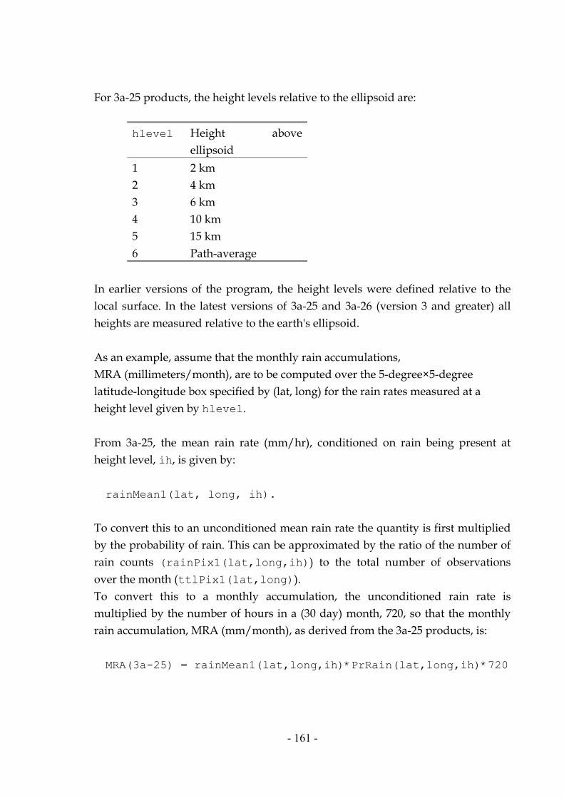
- 161 -
For 3a-25 products, the height levels relative to the ellipsoid are:
hlevel Height above ellipsoid
1 2 km 2 4 km 3 6 km 4 10 km 5 15 km 6 Path-average
In earlier versions of the program, the height levels were defined relative to the local surface. In the latest versions of 3a-25 and 3a-26 (version 3 and greater) all heights are measured relative to the earth's ellipsoid. As an example, assume that the monthly rain accumulations, MRA (millimeters/month), are to be computed over the 5-degree×5-degree latitude-longitude box specified by (lat, long) for the rain rates measured at a height level given by hlevel. From 3a-25, the mean rain rate (mm/hr), conditioned on rain being present at height level, ih, is given by: rainMean1(lat, long, ih).
To convert this to an unconditioned mean rain rate the quantity is first multiplied by the probability of rain. This can be approximated by the ratio of the number of rain counts (rainPix1(lat,long,ih)) to the total number of observations over the month (ttlPix1(lat,long)). To convert this to a monthly accumulation, the unconditioned rain rate is multiplied by the number of hours in a (30 day) month, 720, so that the monthly rain accumulation, MRA (mm/month), as derived from the 3a-25 products, is: MRA(3a-25) = rainMean1(lat,long,ih)*PrRain(lat,long,ih)*720
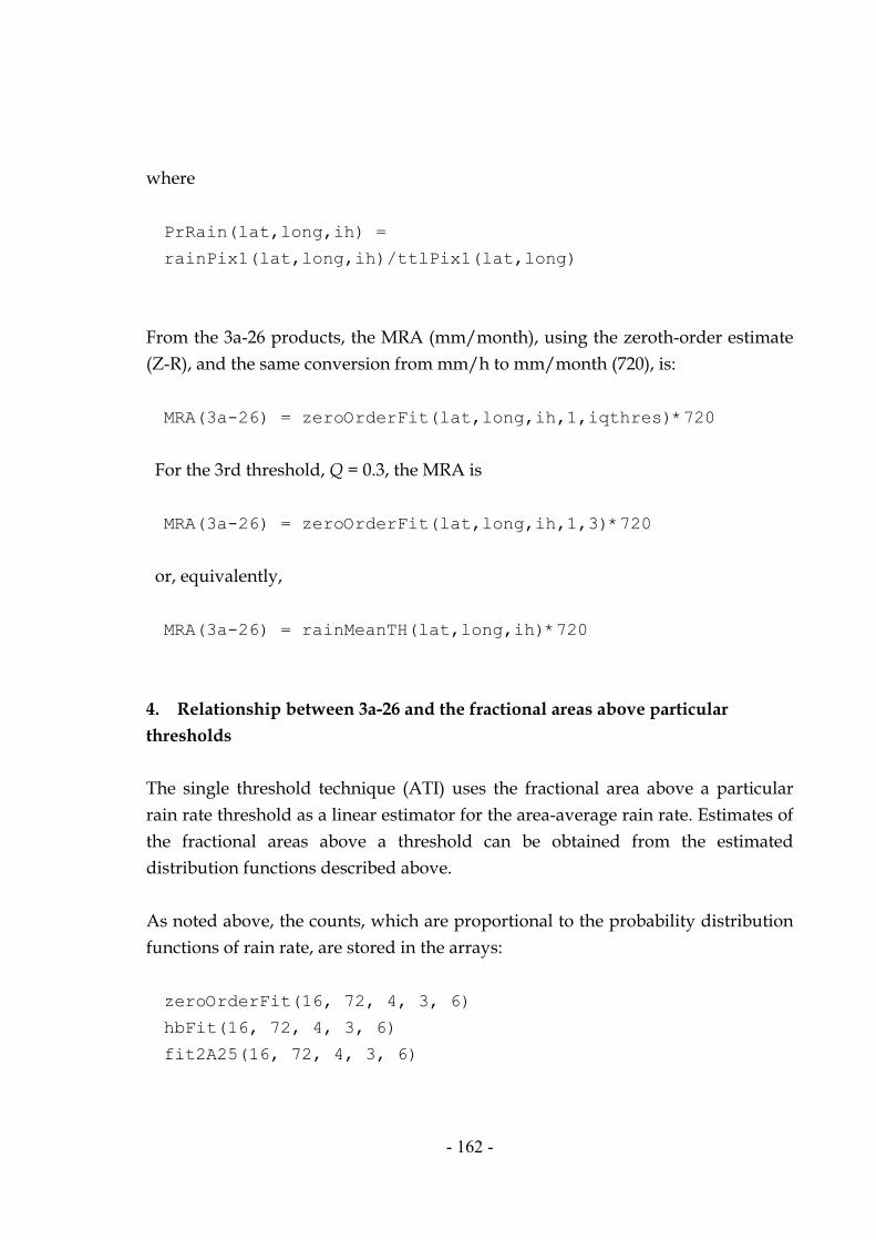
- 162 -
where PrRain(lat,long,ih) =
rainPix1(lat,long,ih)/ttlPix1(lat,long)
From the 3a-26 products, the MRA (mm/month), using the zeroth-order estimate (Z-R), and the same conversion from mm/h to mm/month (720), is: MRA(3a-26) = zeroOrderFit(lat,long,ih,1,iqthres)*720
For the 3rd threshold, Q = 0.3, the MRA is MRA(3a-26) = zeroOrderFit(lat,long,ih,1,3)*720
or, equivalently, MRA(3a-26) = rainMeanTH(lat,long,ih)*720
4. Relationship between 3a-26 and the fractional areas above particular thresholds The single threshold technique (ATI) uses the fractional area above a particular rain rate threshold as a linear estimator for the area-average rain rate. Estimates of the fractional areas above a threshold can be obtained from the estimated distribution functions described above. As noted above, the counts, which are proportional to the probability distribution functions of rain rate, are stored in the arrays: zeroOrderFit(16, 72, 4, 3, 6)
hbFit(16, 72, 4, 3, 6)
fit2A25(16, 72, 4, 3, 6)
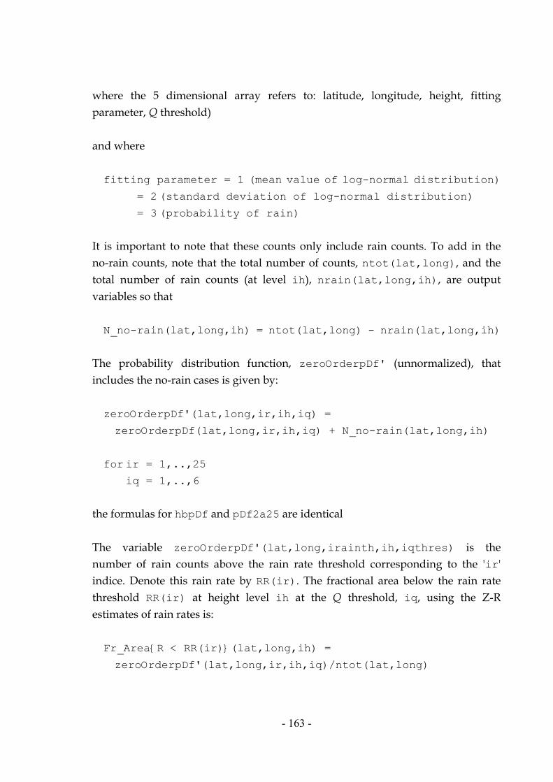
- 163 -
where the 5 dimensional array refers to: latitude, longitude, height, fitting parameter, Q threshold) and where fitting parameter = 1 (mean value of log-normal distribution)
= 2 (standard deviation of log-normal distribution)
= 3 (probability of rain)
It is important to note that these counts only include rain counts. To add in the no-rain counts, note that the total number of counts, ntot(lat,long), and the total number of rain counts (at level ih), nrain(lat,long,ih), are output variables so that N_no-rain(lat,long,ih) = ntot(lat,long) - nrain(lat,long,ih)
The probability distribution function, zeroOrderpDf' (unnormalized), that includes the no-rain cases is given by: zeroOrderpDf'(lat,long,ir,ih,iq) =
zeroOrderpDf(lat,long,ir,ih,iq) + N_no-rain(lat,long,ih)
for ir = 1,..,25
iq = 1,..,6
the formulas for hbpDf and pDf2a25 are identical The variable zeroOrderpDf'(lat,long,irainth,ih,iqthres) is the number of rain counts above the rain rate threshold corresponding to the 'ir' indice. Denote this rain rate by RR(ir). The fractional area below the rain rate threshold RR(ir) at height level ih at the Q threshold, iq, using the Z-R estimates of rain rates is: Fr_Area{R < RR(ir)}(lat,long,ih) =
zeroOrderpDf'(lat,long,ir,ih,iq)/ntot(lat,long)

- 164 -
The fractional area above this threshold is: Fr_Area_RR > RR(ir)(lat,long,ih) =
1 - Fr_Area{R < RR(ir)}(lat,long,ih)
For example, to compute the fractional area above the threshold of 2.05 mm/h (ir = 9 - see definition of the rain rate threshold categories in 3b below) at the Q threshold of 0.9999 (iq = 6) at a height of 2 km above the ellipsoid (ih =1) the following equations are used: zeroOrderpDf'(lat,long,ir=9,ih=1,iq=6) =
zeroOrderpDf(lat,long,ir=9,ih=1,iq=6) +
N_no-rain(lat,long,ih=1)
N_no-rain(lat,long,ih=1) = ntot(lat,long) -
nrain(lat,long,ih=1)
Fr_Area{RR<2.05}(lat,long,ih=1) =
zeroOrderpDf'(lat,long,ir=9,ih=1,iq=6)/ntot(lat,long)
Fr_Area{RR>2.05}(lat,long,ih=1) =
1 - Fr_Area{RR<2.05}(lat,long,ih=1)
So that the fractional area above 2.05 mm/h over the 5×5-degree box (lat, long) over the month (which uses the Z-R derived rain rates and nearly all the data, iq = 6) can be expressed in terms of the HDF outputs: zeroOrderpDf(lat,long,ir=9,ih=1,iq=6)
nrain(lat,long,ih=1)
ntot(lat,long)

- 165 -
5. Reliability estimates
The reliability is defined as the rms difference between experimentally determined values of the pDf and the fitted values of the pDf at those values for which the experimentally-determined pDf increases monontonically. reliabZeroOrder(16,72,4,6)
reliabHB(16,72,4,6)
reliabSRT(16,72,4,6)
if the number of data points is too few or an error occurs in the fitting procedure, the following default values for reliab* and *Fit will be used:
if too few rain occurrences lat-long box, (nrain <200 .and. nrain ≠ 0) then *Fit and reliab* will be set to -999. if number of data points < 2× number of unknowns or if the number of threshold levels is too few or if warning or fatal error occurs in the fitting then *Fit and reliab* will be set to -777. if unconditioned mean rain rate > 3 mm/h and distribution at R = 0.1 mm/h is concave (positive 2nd derivative) then reliab* set to -888 but *Fit parameters are output in normal fashion if unconditioned mean rain rate > 3 mm/h and distribution at R = 0.1 mm/h is convex (negative 2nd derivative) then reliab* set to -555 and *Fit parameters are output in normal fashion if distribution at R = 0.1 mm/h is convex (negative 2nd derivative) and unconditioned mean ≤ 3 see section 11.vi.

- 166 -
6. Definition of the latitude-longitude boxes
The products are defined on a 5-degree×5-degree×1 month grid that covers the TRMM orbit. The latitude boxes are labeled from 1 to 36 where box 1 covers from 40 S to 35 S and box 36 covers from 35 N to 40 N. The longitude boxes are labeled from 1 to 72 where box 1 runs from 180 W to 175 W and box 72 runs from 175 E to 179.999 E. 7. Notes on the processing procedure
1. Assume that 1 granule of data corresponds to 1 orbit.
2. The program is set up to read a scan line of data at a time from 1C-21, 2A-21,
2A-23 and 2A-25 until the full granule of data has been processed.
3. As all the output products are over a 5-degree×5-degree×1 month space-time region, after each granule is processed, the program will write the partially accumulated products to temporary storage. When the next processing cycle begins, these products will be read from temporary storage, and then overwritten once the updated statistics are completed.
4. At the end of the processing cycle (1 month), a subroutine within the
program will be used to output the statistics to the HDF file.
5. For the 0th and HB estimates of rain rate, the EDR (effective dynamic range) is based on the quantity zeta (as defined in 2a-25) or Q (as defined in 3a-26), where:
Q = ζ = 0.2lnβ αZmβ
0
r
∫
where Zm is the measured or apparent reflectivity factor, k = αZ β , and k is the attenuation coefficient or specific attenuation (dB/km), and Z is the actual reflectivity factor (mm6/m3). The coefficients α, and β are read from the 2a-25 output. Note that as Q = ζ goes to one, the path-integrated-attenuation (pia) increases without bound if k-Z relationship is exact. As noted above, the 3a-26 products are defined for height levels of 2 km, 4 km, and 6 km referenced to the ellipsoid. For a height of 2 km, for example, r is that range gate the center of which is closest to the surface drawn 2 km above the ellipsoid.

- 167 -
6. For the multiple threshold method, a necessary condition is that the random variable (that characterizes the radar-measured quantity) be a monotonic function of the quantity that we wish to measure. For example, in the presence of attenuation, the apparent reflectivity factor at the surface Zm(surface) [or the rain rate estimate based on Zm] is a non-monotonic function of the true rain rate; as such it is not an appropriate choice for this method. On the other hand, Q (or ζ) is a monotonic function of the path-integrated rain rate and is appropriate for the 0th order and HB estimates of RR.
7. For the path-integrated attenuation (PIA) as derived from the surface
reference technique (and the corresponding rain rate), an appropriate proxy variable is the SRT estimate of PIA itself. Results based on the SRT are output only to diagnostic file.
8. The motivating principle of the multiple threshold method is that for
area-wide estimates of the rain rate it is more accurate to extrapolate to the low and high regions of rain rate than to attempt to measure the distribution of these values directly. Reasons for the possible poor performance of the radar at high and low rain rates are: i. low SNR at low rain rates ii. signal attenuation at high rain rates iii. higher variability in Z-R laws at low rain rates
9. In the multiple threshold method, an effective dynamic range (EDR) is selected. the EDR is defined as the region over which the rain rates or Zm estimates are expected to have the highest accuracy (where the signal-to-noise ratio is high and attenuation is low).
10. Currently, the maximum number of thresholds within the EDR is taken to
be 25 (the optimum number is still an issue and will depend upon the number of samples and the range of the variable).
11. If the number of samples of the histogram is small, then the estimated pDf
is generally unreliable. To circumvent this, we assume that the total number of IFOVs over the averaging domain, with rain present be larger than some number, iqqmin. Presently, iqqmin = 200.

- 168 -
8. Input Parameters (initialized in 3a-26)
Thresholds: data QUthres0th /0.1,0.2,0.3,0.5,0.75,0.9999/ ! Q-thresholds for Z-R and 2a-25
data QUthresHB /0.1,0.2,0.3,0.5,0.75,0.9999/ ! Q-thresholds for HB
data QLsrt /1.5,1.,0.8,0.6,0.4,0.1/ ! PIA-thresholds for SRT The rain rate distribution functions consist of the count values in the following 25 rain rate categories
data RRcategories ! In mm/hr /0.205, 0.27, 0.3646, 0.4863, 0.648, 0.865, 1.153, 1.537, 2.050, 2.734, 3.646, 4.862, 6.484, 8.6468, 11.531, 15.376, 20.505, 27.344, 36.463, 48.625, 64.84, 86.47, 115.31, 153.76, 205.048/
At present, a lognormal fitting through the points of the rain rates distribution is made only when the following condition is satisfied: iqqmin = 200 ! Minimum number of valid rain occurrences needed for fitting to be done. In identifying the number of valid thresholds, we require that the count value increase by a certain amount from between successive rain rates thresholds; in fact, the upper rain rate threshold can be identified as that threshold beyond which the count value does not increase by at least nfu counts, where:
nfu = 30

- 169 -
9. Output Variables
Arrays for the calculation of probabilities [int*4].
ttlCount(16,72) Number of observations at each 5×5-degree box over the month.
rainCount(16,72,4)
Number of rain observations at each 5×5-degree box over the month. Note that all height levels are measured relative to the ellipsoid.
nrain(i,j,1) h = 2 km nrain(i,j,2) h = 4 km nrain(i,j,3) h = 6 km nrain(i,j,4) path-averaged
Arrays for output of “truncated” histograms at each 5×5×1 month box for 3 RR
estimates/4 “levels”.
zeroOrderpDf(16,72,25,4,6) Number of counts in the probability distribution function (25 categories) using 0th order (Z-R) rain rate estimate at heights with respect to the ellipsoid of 2, 4, 6 km and path-av for 6 Q thresholds.
hbpDf(16,72,25,4,6) Same as above except using the HB estimate of rain rate.
pDf2A25(16,72,25,4,6) Same as above except using the rain rate estimates from 2a-25.

- 170 -
Convention for zeroOrderpDf(16,72,25,4,6), hbpDf(16,72,25,4,6), and pDf2A25(16,72,25,4,6) first argument: latitude second: longitude third: rain rate category for pDf fourth: height “level”: 1 = RR @ 2 km 2 = RR @ 4 km 3 = RR @ 6 km 4 = path-averaged RR fifth: Q threshold
Mean, std dev, Pr(Rain) derived from log-normal assumption to rain rate distribution
zeroOrderFit(16,72,4,3,6) 3 statistics [mean, std dev, Pr(R)] of distribution fit of the rain rates as derived from the 0th (Z-R) method for 6 thresholds at 4 “levels”.
hbFit(16,72,4,3,6) Same as above except Hitschfeld-Bordan method used for rain rate estimates.
fit2A25(16,72,4,3,6) Same as above except data from 2a-25 are used for rain rates estimates.
Reliability factors:
reliabOrderFit(16,72,4,6) reliabHBfit(16,72,4,6) reliab2A25fit(16,72,4,6)
See section 3.2.1.4 for details on computation of the reliability factors.

- 171 -
10. Processing Procedure The basic steps in the procedure are (first 4 are similar to 3a-25 algorithm):
i. Read in data (scan by scan) from 2a-21, 2a-23, 2a-25 and 1c-21
ii. Adjust the range gate numbering conventions so that Zm, Zt and R are aligned properly
iii. Find the coarse boxes to which the 49 IFOVs belong (coarse resolution
boxes are 5-degree×5-degree latitude-longitude boxes)
iv. Resample Zm, Zt and R from the range direction onto the vertical
v. Update the estimated probability distribution function for the various rain rate methods at each 5×5-degree box at the various heights, and for threshold values.
vi. If the granule crosses the month boundary, do a nonlinear least squares
fit to the distributions determined in step 5, assuming a log-normal distribution; from the fitting parameters, calculate the mean, standard deviation and probability of rain for each distribution.
vii. Re- initialize the intermediate file
11. Comments and Issues
i. It is assumed in the program that the verification file does not exist; if it already exists an error will occur.
ii. Differences exists between the height levels at which the 3a-25 and 3a-26
statistics are calculated; for 3a-25 the levels are [2, 4, 6, 10, 15] km and the path-average while for 3a-26 the levels are [2, 4, 6] km and the path-average.
iii. Presently, the height levels are being defined relative to the ellipsoid
and not the local surface.
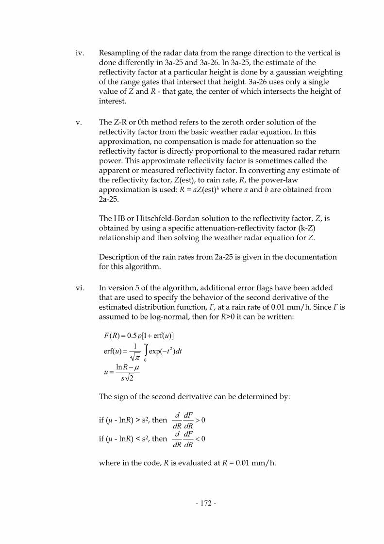
- 172 -
iv. Resampling of the radar data from the range direction to the vertical is done differently in 3a-25 and 3a-26. In 3a-25, the estimate of the reflectivity factor at a particular height is done by a gaussian weighting of the range gates that intersect that height. 3a-26 uses only a single value of Z and R - that gate, the center of which intersects the height of interest.
v. The Z-R or 0th method refers to the zeroth order solution of the
reflectivity factor from the basic weather radar equation. In this approximation, no compensation is made for attenuation so the reflectivity factor is directly proportional to the measured radar return power. This approximate reflectivity factor is sometimes called the apparent or measured reflectivity factor. In converting any estimate of the reflectivity factor, Z(est), to rain rate, R, the power-law approximation is used: R = aZ(est)b where a and b are obtained from 2a-25. The HB or Hitschfeld-Bordan solution to the reflectivity factor, Z, is obtained by using a specific attenuation-reflectivity factor (k-Z) relationship and then solving the weather radar equation for Z. Description of the rain rates from 2a-25 is given in the documentation for this algorithm.
vi. In version 5 of the algorithm, additional error flags have been added
that are used to specify the behavior of the second derivative of the estimated distribution function, F, at a rain rate of 0.01 mm/h. Since F is assumed to be log-normal, then for R>0 it can be written: F(R) = 0.5 p[1+ erf(u)]
erf(u) =1π
exp(−t 2)dt0
u
∫
u =lnR − µ
s 2
The sign of the second derivative can be determined by:
if (µ - lnR) > s2, then ddR
dFdR
> 0
if (µ - lnR) < s2, then ddR
dFdR
< 0
where in the code, R is evaluated at R = 0.01 mm/h.
- 173 -
If ddR
dFdR
< 0 , then an error flag is set (see above).
The following rule can be shown to give a more stable estimate of rain rate:
Begin with Q = 0.3 and evaluate ddR
dFdR
. If this is greater than 0 then
accept the parameters of this distribution. However, if ddR
dFdR
< 0 ,
increase Q and evaluate ddR
dFdR
again; continue this until a Q is found
for which ddR
dFdR
> 0 at which point accept the corresponding
distribution. 12. References [1] Meneghini, R., 1998, J. Appl. Meteor., 37, 924-938. [2] Meneghini, R., and J. Jones, 1993, J. Appl. Meteor., 32, 386-398. [3] Short, D.A., K. Shimizu, B. Kedem, 1993, J. Appl. Meteor., 32, 182-192. [4] Kedem, B., L.S. Chiu, G.R. North, 1990, J. Geophys. Res., 96, 1965-1972. [5] Atlas, D., D. Rosenfeld, D.A. Short, 1990, J. Geophys. Res., 95, 2153-2160. [6] Meneghini, R., J.A. Jones, T. Iguchi, K. Okamoto, and J. Kwiatkowski, 2001, J. Appl. Meteor., 40, 568-585.

- 174 -
PR Team Members
PR Team Leader:
Ken'ichi Okamoto Department of Aerospace Engineering Graduate School Osaka Prefecture University 1-1 Gakuen-cho, Sakai, Osaka 599-8531 Japan Phone: +81-72-254-9241 Fax: +81-72-254-9241 e-mail: [email protected]
1B21, 1C21 Algorithm Developers:
Nobuhiro Takahashi National Institute of Information and Communications Technology 4-2-1 Nukui-Kitamachi, Koganei, Tokyo 184-8795 Japan Phone: +81-42-327-6179 Fax: +81-42-327-6666 e-mail: [email protected]
Shuji Shimizu
JAXA Earth Observation Research and application Center Harumi-Island Triton Square Office tower-X 22F, 1-8-10 Harumi, Chuo-ku, Tokyo 104-6023 Japan Phone: +81-3-6221-9049 Fax: +81-3-6221-9192 e-mail: [email protected]
Jun Awaka
Hokkaido Tokai University 5-1-1-1, Minami-sawa, Minami-ku, Sapporo 005-0825 Japan Phone: +81-11-571-5111 Fax: +81-11-571-7879 e-mail: [email protected]
Toshio Iguchi
National Institute of Information and Communications Technology 4-2-1 Nukui-Kitamachi, Koganei, Tokyo 184-8795 Japan Phone: +81-42-327-7543 Fax: +81-42-327-6666 e-mail: [email protected]

- 175 -
2A21, 3A25, 3A26 Algorithm Developer:
Robert Meneghini NASA Goddard Space Flight Center Code 975, Greenbelt, Maryland 20771 USA Phone: +1-301-286-9128 Fax: +1-301-286-0294 e-mail: [email protected]
2A23 Algorithm Developer:
Jun Awaka Hokkaido Tokai University 5-1-1-1, Minami-sawa, Minami-ku, Sapporo 005-0825 Japan Phone: +81-11-571-5111 Fax: +81-11-571-7879 e-mail: [email protected]
2A25 Algorithm Developer:
Toshio Iguchi National Institute of Information and Communications Technology 4-2-1 Nukui-Kitamachi, Koganei, Tokyo 184-8795 Japan Phone: +81-42-327-7543 Fax: +81-42-327-6666 e-mail: [email protected]