true cosmic microwave background power spectrum estimation

HAL Id: hal-00812427https://hal.archives-ouvertes.fr/hal-00812427

Submitted on 12 Apr 2013

HAL is a multi-disciplinary open accessarchive for the deposit and dissemination of sci-entific research documents, whether they are pub-lished or not. The documents may come fromteaching and research institutions in France orabroad, or from public or private research centers.

L’archive ouverte pluridisciplinaire HAL, estdestinée au dépôt et à la diffusion de documentsscientifiques de niveau recherche, publiés ou non,émanant des établissements d’enseignement et derecherche français ou étrangers, des laboratoirespublics ou privés.

True cosmic microwave background power spectrumestimation

Paniez Paykari, Jean-Luc Starck, Jalal M. Fadili

To cite this version:Paniez Paykari, Jean-Luc Starck, Jalal M. Fadili. True cosmic microwave background power spectrumestimation. Astronomy and Astrophysics - A&A, EDP Sciences, 2012, 541, pp.A74. �10.1051/0004-6361/201118207�. �hal-00812427�

https://hal.archives-ouvertes.fr/hal-00812427

https://hal.archives-ouvertes.fr

True CMB Power Spectrum Estimation

P. Paykari1 ⋆, J.-L. Starck1, and M. J. Fadili2

1 Laboratoire AIM, UMR CEA-CNRS-Paris 7, Irfu, SAp/SEDI, Service d’Astrophysique, CEA Saclay, F-91191 GIF-SUR-YVETTE CEDEX, France.2 GREYC CNRS UMR 6072, ENSICAEN, 6 Bd du Marechal Juin, 14050 Caen Cedex, France

June 29, 2012

ABSTRACT

Context.

Aims. The cosmic microwave background (CMB) power spectrum is a powerful cosmological probe as it entails almostall the statistical information of the CMB perturbations. Having access to only one sky, the CMB power spectrummeasured by our experiments is only a realization of the true underlying angular power spectrum. In this paper we aimto recover the true underlying CMB power spectrum from the one realization that we have without a need to know thecosmological parameters.Methods. The sparsity of the CMB power spectrum is first investigated in two dictionaries; Discrete Cosine Transform(DCT) and Wavelet Transform (WT). The CMB power spectrum can be recovered with only a few percentage of thecoefficients in both of these dictionaries and hence is very compressible in these dictionaries.Results. We study the performance of these dictionaries in smoothing a set of simulated power spectra. Based on this,we develop a technique that estimates the true underlying CMB power spectrum from data, i.e. without a need to knowthe cosmological parameters.Conclusions. This smooth estimated spectrum can be used to simulate CMB maps with similar properties to the trueCMB simulations with the correct cosmological parameters. This allows us to make Monte Carlo simulations in a givenproject, without having to know the cosmological parameters. The developed IDL code, TOUSI, for Theoretical pOwerspectrUm using Sparse estImation, will be released with the next version of ISAP.

Key words. Keywords should be given

Cosmology : Cosmic Microwave Background, Methods : Data Analysis, Methods : Statistical

1. Introduction

Measurements of the CMB anisotropies are powerful cosmological probes. In the currently favored cosmological model,with the nearly Gaussian-distributed curvature perturbations, almost all the statistical information are contained in theCMB angular power spectrum. The observed quantity on the sky is generally the CMB temperature anisotropy Θ(~p) indirection ~p, which is described as T (~p) = TCMB [1 + Θ(~p)]. This field is expanded on the spherical harmonic functions as

Θ(~p) =

+∞∑

ℓ=0

ℓ∑

m=−ℓ

a[ℓ,m]Yℓm(~p) , (1)

where a[ℓ,m] =

∫

S2

Θ(~p)Y ∗

ℓm(~p)d~p , (2)

S2 ⊂ R

3 is the unit sphere, ℓ is the multipole moment which is related to the angular size on the sky as ℓ ∼ 180◦/θ andm is the phase ranging from −ℓ to ℓ. The a[ℓ,m] are the spherical harmonic coefficients of the (noise-free) observed sky.For a Gaussian random field, the mean and covariance are sufficient statistics, meaning that they carry all the statisticalinformation of the field. In case where the random field has zero mean, E(a00) = 0 and the expansion can be startedat ℓ = 2, neglecting the dipole terms, i.e. ℓ = 11. For ℓ > 2, the triangular array (a[ℓ,m])ℓ,m represents zero-mean,complex-valued random coefficients, with variance

E(|a[ℓ,m]|2) = C[ℓ] > 0 , (3)

⋆ [email protected] The dipole anisotropy is dominated by the Earth’s motion in space and it is hence ignored.

2 P. Paykari et al.: True CMB Power Spectrum Estimation

where C[ℓ] is the CMB angular power spectrum, which only depends on ℓ due the isotropy assumption. Therefore, from(3), an unbiased estimator of C[ℓ] is given by the empirical power spectrum

C[ℓ] =1

2ℓ+ 1

∑

m

|a[ℓ,m]|2 . (4)

Furthermore, as the random field is stationary, the spherical harmonic coefficients are uncorrelated,

E(a[ℓ,m]a∗[ℓ′,m′]) = δℓℓ′δmm′C[ℓ] . (5)

Since they are Gaussian they are also independent. The angular power spectrum depends on the cosmological parametersthrough an angular transfer function Tℓ(k) as

C[ℓ] = 4π

∫dk

kT 2

ℓ (k)P (k) , (6)

where k defines the scale and P (k) is the primordial matter power spectrum.Making accurate measurements of this power spectrum has been one of the main goals of cosmology in the past two

decades. We have seen a range of ground- and balloon-based experiments, such as Acbar (Reichardt et al. 2009) and CBI(Readhead et al. 2004), as well as satellite experiments, such as WMAP (Bennett et al. 2003) and the recently launchedsatellite Planck (Planck Collaboration et al. 2011). All these experiments estimate the CMB angular power spectrum froma sky map, which is a realization of the underlying true power spectrum; no matter how much the experiments improve,we are still limited to an accuracy within the cosmic variance. This means that even if we had a perfect experiment (i.e.with zero instrumental noise) we would not be able to recover a perfect power spectrum due to the cosmic variance limit.

In this paper we investigate the possibility of estimating the true underlying power spectrum from a realized spectrum;an estimation of the true power spectrum without a need to know the cosmological parameters. For this we exploit thesparsity properties of the CMB power spectrum, and capitalize on it to propose an estimator of the theoretical powerspectrum. This estimate will not belong to a set of possible theoretical power spectra (i.e. all C[ℓ] that can be obtainedby CAMB2 by varying the cosmological parameters). Instead, such an estimation should be useful for other applications,such as:

• Monte Carlo: we may want to make Monte Carlo simulations in some applications without assuming the cosmologicalparameters.

• Wiener filtering: Wiener filtering is often used to filter the CMB map and it requires the theoretical power spectrumas an input. We may not want to assume any cosmology at this stage of the processing.

• Some estimators (weak lensing, ISW, etc.) require the theoretical power spectrum to be known. Using a data-basedestimation of the theoretical C[ℓ] could be an interesting alternative, or at least a good first guess in an iterativescheme where the theoretical C[ℓ] is required to determine the cosmological parameters.

2. Sparsity of the CMB Power Spectrum

2.1. A brief tour of sparsity

A signal X = (X[1], . . . , X[N ]) considered as a vector in RN , is said to be sparse if most of its entries are equal to zero. If

k number of the N samples are not equal to zero, where k ≪ N , then the signal is said to be k-sparse. In the case whereonly a few of the entries have large values and the rest are zero or close to zero the signal is said to be weakly sparse(or compressible). With a slight abuse of terminology, in the sequel, we will call compressible signals sparse. Generallysignals are not sparse in direct space, but can be sparsified by transforming them to another domain. For example, sin(x)is 1-sparse in the Fourier domain, while it is clearly not sparse in the original one. In the so-called sparsity synthesismodel, a signal can be represented as the linear expansion

X = Φα =

T∑

i=1

φiα[i] , (7)

where α[i] are the synthesis coefficients of X, Φ = (φ1, . . . , φT ) is the dictionary, and φi are called the atoms (elementarywaveforms) of the dictionary Φ. In the language of linear algebra, the dictionary Φ is a N ×T matrix whose columns are

the atoms normalized, supposed here to be normalized to a unit ℓ2-norm, i.e. ∀i ∈ [1, T ], ‖φi‖22 =

∑Nn=1 |φi[n]|2 = 13. A

function can be decomposed in many dictionaries, but the best dictionary is the one with the sparsest (most economical)representation of the signal. In practice, it is convenient to use dictionaries with fast implicit transform (such as Fouriertransform, wavelet transform, etc.) which allow us to directly obtain the coefficients and reconstruct the signal fromthese coefficients using fast algorithms running in linear or almost linear time (unlike matrix-vector multiplications).The Fourier, wavelet and discrete cosine transforms provide certainly the most well known dictionaries. A comprehensiveaccount on sparsity and its applications can be found in the monograph (Starck et al. 2010).

2 CAMB solves the Boltzmann equations for a cosmological model set out by the given cosmological parameters.3 The lp-norm of a vector X, p ≥ 1, is defined as ‖X‖p =

`

P

i |X[i]|p´1/p

, with the usual adaptation ‖X‖∞ = maxi X[i].

P. Paykari et al.: True CMB Power Spectrum Estimation 3

2.2. Which Dictionary for the Theoretical CMB Power Spectrum?

We investigate the sparsity of the CMB power spectrum in two different dictionaries, both having a fast implicit transform:the Wavelet Transform (WT) and the Discrete Cosine Transform (DCT).

Fig. 1. A theoretical CMB power spectrum along with the reconstructed power spectra, using the DCT and WT dic-tionaries. The panels show the reconstructions for different fractions of the coefficients used. The inner plots show thedifferences between the actual and the reconstructed power spectra. Both dictionaries suffer from boundary effects, butthis is more severe for DCT as the corresponding atoms are not compactly supported. It is worth mentioning that thepower spectrum that is decomposed onto the two dictionaries is in the form ℓ(ℓ+ 1)C[ℓ]/2π.

Figure 1 shows an angular power spectrum (calculated by CAMB (Lewis et al. 2000) with WMAP7 (Larson et al.2010) parameters) along with the DCT- and WT-reconstructed power spectra with a varying fraction of the largesttransform coefficients retained in the reconstruction. The inner plots show the difference between the actual powerspectrum and the reconstructed ones. It can be seen that with only a few percentage of the coefficients the shape of thepower spectrum is correctly reconstructed in both dictionaries. The height and the position of the peaks and troughsare of great importance here as the estimation of the cosmological parameters heavily relies on these characteristics ofthe power spectrum. The best domain would be the one with the sparsest representation and yet the most accurate

representation of the power spectrum. Let C[ℓ](M)

be its best M -term approximation, i.e. obtained by reconstructingfrom the M -largest (in magnitude) coefficients of C[ℓ] in a given domain. To compare the WT and DCT dictionaries, weplot the resulting non-linear approximation (NLA) error curve in Figure 2, which shows the reconstruction error EM asa function of M , the number of retained coefficients;

EM =

∥∥∥C[ℓ] − C[ℓ](M)

∥∥∥2

‖C[ℓ]‖2

× 100 . (8)

As M increases we get closer to the complete reconstruction and the error reaches 0 when all the coefficients have beenused. Usually the domain with the steepest EM curve is the sparsest domain. In this case though both dictionaries


Fig. 2. Non-Linear Approximation (NLA) error curves for the two dictionaries. Below 1% the DCT curve is droppingfaster, which means it is doing a better job. However, past ∼ 2% the DCT curve flattens off while WT decreases to ∼ 0very quickly.

have very similar behaviors. There is only a small window in the coefficients for which DCT does a better job thanWT. However, DCT flattens after using ∼ 1% of the coefficients and does not improve the reconstruction until a bigproportion of the coefficients have been used.

Both dictionaries seem to suffer from boundary issues at low and high ℓs. This can be solved for high ℓs as onecan always perform the reconstruction beyond the desired ℓ. For low ℓs it can be solved by different means, such asextrapolation of the spectrum. Note that the boundary issues are more severe in the DCT domain than WT; this is dueto the fact that DCT atoms are not compactly supported.

Next we investigate the sparsity of a set of realized spectra in the two dictionaries. We simulate 100 maps from thetheoretical power spectrum used previously and estimate their power spectra using equation 4 . As before, we decomposeeach realization in the DCT and WT dictionaries and reconstruct keeping increasing fractions of the largest coefficients.At this stage, it is important to note that, as we are dealing with the empirical power spectrum, we are no longer inan approximation setting but rather in an estimation one. Indeed, the empirical power spectrum can be seen as a noisyversion of the true one. Intuitively, reconstructing from a very small fraction of high coefficients will reject most of thenoise (low estimator variance) but at the price of retaining only a small fraction of the true spectrum coefficients (largebias). The converse is true when a large proportion of coefficients is kept in the reconstruction. Therefore, there will exista threshold value that will entail a bias-variance tradeoff, hence minimizing the estimation risk. This is exactly the ideaunderlying thresholding estimators in sparsifying domains.

This discussion is clearly illustrated by the inner plots of Figure 3, which shows the normalized mean-square error(NMSE) defined as

NMSEM =

∥∥∥∥C[ℓ] − C[ℓ](M)

∥∥∥∥2

‖C[ℓ]‖2

× 100 , (9)

as a function of the fraction of coefficients used in the reconstruction. The error is large when only a few coefficients areused. As more coefficients are included, one starts to recover the main (i.e. the general shape of the spectrum) features of


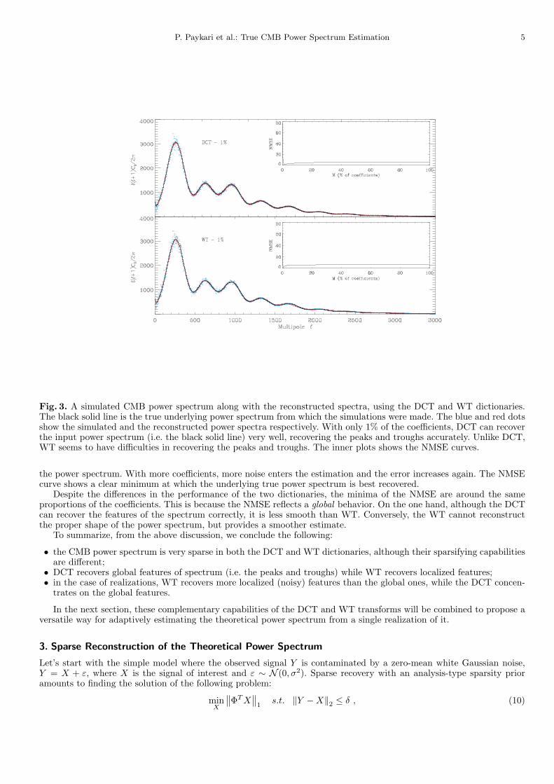
Fig. 3. A simulated CMB power spectrum along with the reconstructed spectra, using the DCT and WT dictionaries.The black solid line is the true underlying power spectrum from which the simulations were made. The blue and red dotsshow the simulated and the reconstructed power spectra respectively. With only 1% of the coefficients, DCT can recoverthe input power spectrum (i.e. the black solid line) very well, recovering the peaks and troughs accurately. Unlike DCT,WT seems to have difficulties in recovering the peaks and troughs. The inner plots shows the NMSE curves.

the power spectrum. With more coefficients, more noise enters the estimation and the error increases again. The NMSEcurve shows a clear minimum at which the underlying true power spectrum is best recovered.

Despite the differences in the performance of the two dictionaries, the minima of the NMSE are around the sameproportions of the coefficients. This is because the NMSE reflects a global behavior. On the one hand, although the DCTcan recover the features of the spectrum correctly, it is less smooth than WT. Conversely, the WT cannot reconstructthe proper shape of the power spectrum, but provides a smoother estimate.

To summarize, from the above discussion, we conclude the following:

• the CMB power spectrum is very sparse in both the DCT and WT dictionaries, although their sparsifying capabilitiesare different;

• DCT recovers global features of spectrum (i.e. the peaks and troughs) while WT recovers localized features;• in the case of realizations, WT recovers more localized (noisy) features than the global ones, while the DCT concen-

trates on the global features.

In the next section, these complementary capabilities of the DCT and WT transforms will be combined to propose aversatile way for adaptively estimating the theoretical power spectrum from a single realization of it.

3. Sparse Reconstruction of the Theoretical Power Spectrum

Let’s start with the simple model where the observed signal Y is contaminated by a zero-mean white Gaussian noise,Y = X + ε, where X is the signal of interest and ε ∼ N (0, σ2). Sparse recovery with an analysis-type sparsity prioramounts to finding the solution of the following problem:

minX

∥∥ΦTX∥∥

1s.t. ‖Y −X‖2 ≤ δ , (10)


where ΦTX represent the transform coefficients of X in the dictionary Φ, and δ controls the fidelity to the data andobviously depends on the noise standard deviation σ.

Let’s now turn to denoising the power spectrum from one empirical realization of it. In this case, however, the noiseis highly non-Gaussian and needs to be treated differently. Indeed, as we will see in the next section, the empirical powerspectrum will entail a multiplicative χ2-distributed noise with a number of degrees of freedom that depends on ℓ. Thatis, the noise has a variance profile that dependents both on the true spectrum and ℓ. We therefore need to stabilize thenoise on the empirical power spectrum prior to estimation, using a Variance Stabilization Transform (VST). Hopefully,the latter will yield stabilized samples that have (asymptotically) constant variance, say 1, irrespective of the value ofthe input noise level.

3.1. Variance Stabilizing Transform

In the statistical literature the problem of removing the noise from an empirical power spectrum goes by the name ofperiodogram denoising (Donoho 1993). In (Komm et al. 1999), approximating the noise with a correlated Gaussian noisemodel, a threshold was derived at each wavelet scale using the MAD (Median of Absolute Deviation) estimator. A moreelegant approach was proposed in (Donoho 1993; Moulin 1994), where the so-called Wahba VST was used. This VST isdefined as:

T (X) = (logX + γ)

√6

π, (11)

where γ = 0.57721... is the Euler-Mascheroni constant. After the VST, the stabilized samples can be treated as if thenoise contaminating them were white Gaussian noise with unit variance.

We will take a similar path here, generalizing the above approach to the case of the angular power spectrum. Indeed,from (4), one can show that under mild regularity assumptions on the true power spectrum,

C[ℓ]d→ C[ℓ]Z[ℓ], where ∀ℓ ≥ 2, 2LZ[ℓ] ∼ χ2

2L, L = 2ℓ+ 1 . (12)

d→ means convergence in distribution. From (12), it is appealing then to take the logarithm so as to transform themultiplicative noise Z into an additive one. The resulting log-stabilized empirical power spectrum reads

Cs[ℓ] := Tℓ(C[ℓ]) = log C[ℓ] − µL = logC[ℓ] + η[ℓ] . (13)

where η[ℓ] := logZ[ℓ] − µL, L = 2ℓ + 1. Using the asymptotic results from (Bartlett & Kendall 1946) on the momentsof log−χ2 variables, it can be shown that µL = ψ0 (L) − logL, E(η[ℓ]) = 0 and σ2

L = Var [η[ℓ]] = ψ1 (L), where ψm(t) is

the standard polygamma function, ψm(t) = dm+1

dtm+1 log Γ(t).We can now consider the stabilized Cs[ℓ] as noisy versions of the logC[ℓ], where the noise is zero-mean additive and

independent. Owing to the Central Limit Theorem, the noise tends to Gaussian with variance σ2L as ℓ increases. At low

ℓ, normality is only an approximation. In fact, it can be show that the noise η[ℓ] has a probability density function ofthe form

pη(ℓ) =(2L)L

2LΓ(L)exp

[L

(ℓ+ µL − eℓ+µL

)], (14)

which might be used to estimate the thresholds in the wavelet domain.In order to standardize the noise, the VST (13) will be slightly modified to the normalized form

Cs[ℓ] := Tℓ(C[ℓ]) =log C[ℓ] − µL

σL

= Xs[ℓ] + ε[ℓ] . (15)

where now the noise ε[ℓ] is zero-mean (asymptotically) Gaussian with unit variance, and Xs[ℓ] := logC[ℓ]/σL. It can bechecked that the Wahba VST (11) is a specialization of (15) to L = 0.

In the following, we will use the operator notation T (X) for the VST that applies (15) entry-wise to each X[ℓ], andR(X) its inverse operator, i.e. R(X) :=

(Rℓ(X[ℓ])

)ℓ

with Rℓ(X[ℓ]) = exp(σLX[ℓ]).

3.2. Signal detection in the wavelet domain

Without of loss of generality, we restrict our description here to the wavelet transform. The same approach applies toother sparsifying transforms, e.g. DCT, just as well.

In order to estimate the true CMB power spectrum from the wavelet transform, it is important to detect the waveletcoefficients which are “significant”, i.e. the wavelet coefficients which have an absolute value too large to be due to noise(cosmic variance + instrumental noise). Let wj [ℓ] the wavelet coefficient of a signal Y at scale j and location ℓ. We definethe multiresolution support M of Y as:

Mj [ℓ] =

{1 if wj [ℓ] is significant,

0 if wj [ℓ] otherwise.(16)


For Gaussian noise, it is easy to derive an estimation of the noise standard deviation σj at scale j from the noise standarddeviation, which can be evaluated with good accuracy in an automated way (Starck & Murtagh 1998). To detect thesignificant wavelet coefficients, it suffices to compare the wavelet coefficients in magnitude |wj [ℓ]| to a threshold level tj .This threshold is generally taken to be equal to κσj , where κ ranges from 3 to 5. This means that a small magnitudecompared to the threshold implies that the coefficients is very likely to be due to noise and hence insignificant. Such adecision rule corresponds to the hard-thresholding operator

if |wj [ℓ]| ≥ tj then wj [ℓ] is significant ,if |wj [ℓ]| < tj then wj [ℓ] is not significant.

(17)

To summarize, The multiresolution support is obtained from the signal Y by computing the forward transformcoefficients, applying hard thresholding, and recording the coordinates of the retained coefficients.

3.3. Power Spectrum Recovery Algorithm

Let’s now turn to the adaptive estimator of the true CMB power spectrum C[ℓ] from its empirical estimate C[ℓ]. As webenefit from the (asymptotic) normality of the noise in the stabilized samples Cs[ℓ] in (15), we are in position to easilyconstruct the multiresolution support M of Cs as described in the previous section. Once the support M of significant

coefficients has been determined, our goal is reconstruct an estimate X of the true power spectrum, known to be sparselyrepresented in some dictionary Φ(regularization), such that the significant transform coefficients of its stabilized versionreproduce those of Cs (fidelity to data). Furthermore, as a power spectrum is a positive, a positivity constraint mustbe imposed. These requirements can be cast as seeking an estimate that solves the following constrained optimizationproblem:

minX

‖ΦTX‖1 s.t.

{X > 0

M ⊙(ΦTT (X)

)= M ⊙

(ΦTCs

) , (18)

where ⊙ stands for the Hadamard product (i.e. entry-wise multiplication) of two vectors. This problem has a globalminimizer which is bounded. However, beside non-smoothness of the l1-norm and the constraints, the problem is alsonon-convex because of the VST operator T . It is therefore far from obvious to solve.

In this paper we propose the following scheme which starts with an initial guess of the power spectrum X(0) = 0, andthen iterates for n = 0 to Nmax − 1,

X = R(T

(X(n)

)+ ΦM ⊙

(ΦT

(Cs − T

(X(n)

))))

X(n+1) = P+

(Φ STλn

(ΦT X)),

(19)

where P+ denotes the projection on the positive orthant and guarantees non-negativity of the spectrum estimator,STλn

(w) = (STλn(w[i]))i is the soft-thresholding with threshold λn that applies term-by-term the shrinkage rule

STλn(w[i]) =

{sign(w[i])(|w[i]| − λn) if |w[i]| > λn ,

0 otherwise .(20)

Here, we have chosen a decreasing threshold with the iteration number n, λn = (Nmax − n)/(Nmax − 1). More detailspertaining to this algorithm can be found in Starck et al. (2010)

3.4. Instrumental Noise

In practice, the data are generally contaminated by an instrumental noise, and estimating the true CMB power spectrum

C[ℓ] from the empirical power spectrum C[ℓ] requires to remove this instrumental noise. The instrumental noise isassumed stationary and independent from the CMB. We will also suppose that we have access to the power spectrum

of the noise, or we can compute the empirical power spectrum SN [ℓ] of at least one realization, either from a JackKnifedata map or from realistic instrumental noise simulations. The above algorithm can be adapted to handle this case afterrewriting the optimizing problem as follows:

minX

‖ΦTX‖1 s.t.

{X > 0

M ⊙(ΦTT (X + SN )

)= M ⊙

(ΦTCs

) . (21)

Thus, (19) becomes

X = R(T

(X(n) + SN

)+ ΦM ⊙

(ΦT

(Cs − T

(X(n) + SN

))))− SN

X(n+1) = P+

(Φ STλn

(ΦT X)).

(22)


3.5. Combining Several Dictionnaries

We have seen in Section 2.2 that the WT and DCT dictionaries had complementary benefits. Indeed each dictionaryis able to capture well features with shapes similar to its atoms. More generally, assume that we have D dictionariesΦ1, · · · ,ΦD. Given a candidate signal Y , we can derive a support Md associated to each dictionary Φd, for d ∈ {1, · · · , D}.The optimization problem to solve now reads

minX

‖ΦTX‖1 s.t.

{X > 0

Md ⊙(ΦT

d T (X + SN ))

= Md ⊙(ΦT

dCs), d ∈ {1, · · · , D} . (23)

Again, this is a challenging optimization problem. We propose to attack it by applying successively and alternatively(22) on each dictionary Φd. Algorithm 1 describes in detail the different steps.

Algorithm 1: TOUSI Power Spectrum Smoothing with D dictionaries

Require:

Empirical power spectrum bC, D dictionaries Φ1, ..., ΦD, noise power spectrum bSN ,Number of iterations Nmax,Threshold κ (default value is 5).Detection

1: Compute Cs using (15).2: For all d, compute the decomposition coefficients Wd of Cs in Φd, Wd = ΦT

d Cs.3: For all d, compute the support Md from Wd with the threshold κ, assuming standard additive white Gaussian noise.

Estimation

4: Initialize X(0) = 0,5: for n = 0 to Nmax − 1 do6: Zd = X(n).7: for d = 1 to D do

8: eZ = R“

T“

Zd + bSN

”

+ ΦdM ⊙“

ΦdT

“

Cs − T“

Zd + bSN

””””

− bSN .

9: Zd+1 = P+

“

Φd STλn(Φd

TeZ)

”

.

10: end for11: X(n+1) = ZD+1.12: λn+1 = Nmax−(n+1)

Nmax−1.

13: end for14: Get the estimate eX = X(Nmax).

4. Data with Instrumental Noise

Here we present the performance of the TOUSI algorithm in the presence of instrumental noise. The noise maps weresimulated using a theoretical (PLANCK level) noise power spectrum. They were added to the CMB maps simulatedpreviously and the power spectra of the combined maps were estimated using equation 4.

Figure 4 shows the reconstruction of the theoretical CMB spectrum in the presence of noise. The blue dots show theempirical power spectrum of one realization having instrumental noise. Yellow dots show the estimated power spectrumof one of the simulated noise maps. Green dots show the the spectrum with the noise power spectrum removed. Theblack and red solid lines are the input and reconstructed power spectra respectively. The theoretical power spectrum canbe reconstructed up to the point where the structure of the power spectrum has not been destroyed by the instrumentalnoise. In our case, having PLANCK level noise, this goes to ℓ up to 2500. It can be seen that TOUSI can do a great jobin reconstructing the input power spectrum even in the presence of instrumental noise.

5. Sparsity versus Averaging

A very common approach to reduce the noise on the power spectrum is the moving average filter, i.e. average values ina given window,

CA[b] =1

b(b+ 1)ωb

b+ωb

2∑

ℓ=b−ωb

2

ℓ(ℓ+ 1)C[ℓ] , (24)

and the window size ωb is increasing with ℓ. Here, we use window sizes of {1, 2, 5, 10, 20, 50, 100} respectively for ℓ rangingfrom {2, 11, 31, 151, 421, 1201, 2501} to {10, 30, 150, 420, 1200, 2500, 3200}, which have also been used in the framework ofthe PLANCK project in (Leach et al. 2008).


Fig. 4. Power spectrum estimation in the presence of instrumental noise. The blue dots show the empirical powerspectrum of one realization having instrumental noise. Yellow dots show the estimated power spectrum of one of thesimulated noise maps. Green dots show the the spectrum with the noise power spectrum removed. The black and redsolid lines are the input and reconstructed power spectra respectively. The inner plots show a zoomed-in version.

Figure 5 shows the average error the 100 realizations as a function of ℓ

E[ℓ] =1

100

100∑

i=1

‖ C[ℓ] − Ci[ℓ] ‖2 , (25)

where Ci is the estimated power spectrum from the i-th realization. We display the errors for the spectra estimated bythe empirical estimator (the realization, black dotted line), the averaging estimator (red dashed line) and TOUSI (solidblue line). The cosmic variance is over-plotted as a solid black line. We can see that the expected error is highly reducedwhen using the sparsity-based estimator.

6. Conclusion

Measurements of the CMB anisotropies are powerful cosmological probes. In the currently favored cosmological model,with the nearly Gaussian-distributed curvature perturbations, almost all the statistical information are contained inthe CMB angular power spectrum. In this paper we have investigated the sparsity of the CMB power spectrum in twodictionaries; DCT and WT. In both dictionaries the CMB power spectrum can be recovered with only a few percentagesof the coefficients, meaning the spectrum is very sparse. The two dictionaries have different characteristics and canaccommodate reconstructing different features of the spectra; The DCT can help recover the global features of thespectrum, while WT helps recover small localized features. The sparsity of the CMB spectrum in these two domainshas helped us develop an algorithm, TOUSI, that estimates the true underlying power spectrum from a given realizedspectrum. This algorithm uses the sparsity of the CMB power spectrum in both WT and DCT domains and takes thebest from both worlds to get a highly accurate estimate from a single realization of the CMB power spectrum. This couldbe a replacement for CAMB in cases where knowing the cosmological parameters is not necessary. The developed IDLcode will be released with the next version of ISAP (Interactive Sparse astronomical data Analysis Packages) via theweb site:

http://jstarck.free.fr/isap.html


Fig. 5. Mean error for the 100 realizations, for the realizations (black dotted line), the averaging denoising (red dashedline) and the sparse wavelet filtering (blue solid line). The inner plot shows a zoom between l = 2000 and l = 3000.

Acknowledgments

The authors would like to thank Marian Douspis, Olivier Dore and Amir Hajian for useful discussions. This work issupported by the European Research Council grant SparseAstro (ERC-228261)

References

Bartlett, M. S. & Kendall, D. G. 1946, Journal of the Royal Statistical Society, Series B, 8, 128Bennett, C. L., Hill, R. S., Hinshaw, G., et al. 2003, APJS, 148, 97Donoho, D. 1993, in Proceedings of Symposia in Applied Mathematics, ed. A. M. Society, Vol. 47, 173–205Komm, R. W., Gu, Y., Hill, F., Stark, P. B., & Fodor, I. K. 1999, ApJ, 519, 407Larson, D., Dunkley, J., Hinshaw, G., et al. 2010, ArXiv e-printsLeach, S. M., Cardoso, J.-F., Baccigalupi, C., et al. 2008, A&A, 491, 597-615Lewis, A., Challinor, A., & Lasenby, A. 2000, Astrophys. J., 538, 473Moulin, P. 1994, IEEE Transactions on Signal Processing, 42, 3126–3136Planck Collaboration, Ade, P. A. R., Aghanim, N., et al. 2011, ArXiv e-printsReadhead, A. C. S., Mason, B. S., Contaldi, C. R., et al. 2004, APJ, 609, 498Reichardt, C. L., Ade, P. A. R., Bock, J. J., et al. 2009, APJ, 694, 1200Starck, J.-L. & Murtagh, F. 1998, Publications of the Astronomical Society of the Pacific, 110, 193-199Starck, J.-L., Murtagh, F., & Fadili, M. 2010, Sparse Image and Signal Processing (Cambridge University Press)

true cosmic microwave background power spectrum estimation

Documents