tu darmstadt einführung in die künstliche intelligenz outline · chess, checkers, othello,...
TRANSCRIPT

Game Playing: Adversarial Search
TU Darmstadt Einführung in die Künstliche Intelligenz
V2.1 | J. Fürnkranz1
Outline Introduction
What are games and why are they interesting? History and State-of-the-art in Game Playing
Game-Tree Search Minimax Negamax α-β pruning
Real-time Game-Tree Search NegaScout evaluation functions practical enhancements selective search
Multiplayer Game Trees Many slides based on Russell & Norvig's slidesArtificial Intelligence:A Modern Approach

Game Playing: Adversarial Search
TU Darmstadt Einführung in die Künstliche Intelligenz
V2.0 | J. Fürnkranz2
What are and why study games? Games are a form of multi-agent environment
What do other agents do and how do they affect our success? Cooperative vs. competitive multi-agent environments. Competitive multi-agent environments give rise to adversarial
search a.k.a. games
Why study games? Fun; historically entertaining Interesting subject of study because they are hard Easy to represent and agents restricted to small number of
actions Problem (and success) is easy to communicate

Game Playing: Adversarial Search
TU Darmstadt Einführung in die Künstliche Intelligenz
V2.0 | J. Fürnkranz3
Relation of Games to Search Search – no adversary
Solution is method for finding goal
Heuristics and CSP techniques can find optimal solution
Evaluation function: estimate of cost from start
to goal through given node
Examples: path planning, scheduling
activities
Games – adversary Solution is strategy
strategy specifies move for every possible opponent reply
Time limits force an approximate solution
Evaluation function: evaluate “goodness” of
game position
Examples: chess, checkers, Othello,
backgammon, ...

Game Playing: Adversarial Search
TU Darmstadt Einführung in die Künstliche Intelligenz
V2.0 | J. Fürnkranz4
Types of Games
deterministic chanceperfect
informationchess, checkers, Go,
Othellobackgammon,
monopoly
imperfect information
battleship, kriegspiel, matching pennies,
Roshambo
bridge, poker, scrabble
Zero-Sum Games one player's gain is the other player's (or players') loss
turn-taking players alternate moves
deterministic games vs. games of chance do random components influence the progress of the game?
perfect vs. imperfect information does every player see the entire game situation?

Game Playing: Adversarial Search
TU Darmstadt Einführung in die Künstliche Intelligenz
V2.0 | J. Fürnkranz5
A Brief History of Search in Game Playing
Computer considers possible lines of play (Babbage, 1846)
Algorithm for perfect play (Zermelo, 1912; Von Neumann, 1944)
Finite horizon, approximate evaluation (Zuse, 1945; Wiener, 1948; Shannon, 1950)
First computer chess game(Turing, 1951)
Machine learning to improve evaluation accuracy (Samuel, 1952-57)
Selective Search Programs(Newell, Shaw, Simon 1958; Greenblatt, Eastake, Crocker 1967)
Pruning to allow deeper search (McCarthy, 1956)
Breakthrough of Brute-Force Programs(Atkin & Slate, 1970-77)

Game Playing: Adversarial Search
TU Darmstadt Einführung in die Künstliche Intelligenz
V2.0 | J. Fürnkranz6
Checkers:Chinook vs. Tinsley
© Jonathan Schaeffer
Name: Marion TinsleyProfession: Teach mathematicsHobby: CheckersRecord: Over 42 years loses only 3 (!) games of checkers

Game Playing: Adversarial Search
TU Darmstadt Einführung in die Künstliche Intelligenz
V2.0 | J. Fürnkranz7
Chinook
First computer to win human world championship!Visit http://www.cs.ualberta.ca/~chinook/ to play a version of Chinook over the Internet.
© Jonathan Schaeffer

Game Playing: Adversarial Search
TU Darmstadt Einführung in die Künstliche Intelligenz
V2.0 | J. Fürnkranz8
Chinook
July 19 2007, after 18 years of computation:http://citeseerx.ist.psu.edu/viewdoc/summary?doi=10.1.1.95.5393

Game Playing: Adversarial Search
TU Darmstadt Einführung in die Künstliche Intelligenz
V2.0 | J. Fürnkranz9
Backgammon
© Jonathan Schaeffer
branching factor several hundred
TD-Gammon v1 –1-step lookahead, learns to play games against itself
TD-Gammon v2.1 –2-ply search, doeswell against world champions
TD-Gammon has changed the way experts play backgammon.

Game Playing: Adversarial Search
TU Darmstadt Einführung in die Künstliche Intelligenz
V2.0 | J. Fürnkranz10
Chess
Kasparov
5’10” 176 lbs 34 years50 billion neurons2 pos/secExtensiveElectrical/chemicalEnormous
Name
HeightWeight
AgeComputers
SpeedKnowledge
Power SourceEgo
Deep Blue
6’ 5”2,400 lbs
4 years512 processors
200,000,000 pos/secPrimitiveElectrical
None
© Jonathan Schaeffer
http://www.wired.com/wired/archive/9.10/chess.htm

Game Playing: Adversarial Search
TU Darmstadt Einführung in die Künstliche Intelligenz
V2.0 | J. Fürnkranz11
Reversi/Othello
© Jonathan Schaeffer
Name: Takeshi MurakamiTitle: World Othello Champion1997: Lost 6-0 against OthelloProgram Logistello

Game Playing: Adversarial Search
TU Darmstadt Einführung in die Künstliche Intelligenz
V2.0 | J. Fürnkranz12
Computer Go
© Jonathan Schaeffer
Name: Chen ZhixingAuthor: Handtalk (Goemate)Profession: RetiredComputer skills: Selftaught assembly language programmerAccomplishments: dominated computer go for 4 years.

Game Playing: Adversarial Search
TU Darmstadt Einführung in die Künstliche Intelligenz
V2.1 | J. Fürnkranz13
Computer Go, early 2000s
© Jonathan Schaeffer
Active Area of research
Methods relying on Monte
Carlo tree search gave a
strong boost in performance,
Best Humans are still out of
reach on the 19x19 board.
Name: Chen ZhixingAuthor: Handtalk (Goemate)Profession: RetiredComputer skills: Selftaught assembly language programmerAccomplishments: dominated computer go for 4 years.
Gave Handtalk a 9 stone handicap and still easily beat the program,thereby winning $15,000

Game Playing: Adversarial Search
TU Darmstadt Einführung in die Künstliche Intelligenz
V1.0 | J. Fürnkranz14
Computer Go, 2016 Oktober 2015:
AlphaGo beats European champion Fan Hui
First win of a computer against a professional Go player
https://gogameguru.com/alpha-go-fan-hui/
March 2016: AlphaGo beats Lee Sedol,
one of the best professional players
Techniques: Combination of Deep Learning,
Reinforcement Learning and Monte-Carlo Tree Search

Game Playing: Adversarial Search
TU Darmstadt Einführung in die Künstliche Intelligenz
V1.0 | J. Fürnkranz15
AlphaZero Improved version of AlphaGo
Also successfully learned to play chess and Shogi (Japanese Chess)
December 2017: AlphaZero beats the strongest programs in all three games
after hours (chess) or days (Go) of training
https://arxiv.org/pdf/1712.01815.pdf

Game Playing: Adversarial Search
TU Darmstadt Einführung in die Künstliche Intelligenz
V2.0 | J. Fürnkranz16
Outline Introduction
What are games? History and State-of-the-art in Game Playing
Game-Tree Search Minimax α-β pruning NegaScout
Real-time Game-Tree Search evaluation functions practical enhancements selective search
Games of imperfect information and games of chance Simulation Search
Monte-Carlo search UCT search

Game Playing: Adversarial Search
TU Darmstadt Einführung in die Künstliche Intelligenz
V2.0 | J. Fürnkranz17
Solving a Game Ultra-weak
prove whether the first player will win, lose, or draw from the initial position, given perfect play on both sides
could be a non-constructive proof, which does not help in play could be done via a complete minimax or alpha-beta search Example:
chess when first move may be a pass Weak
provide an algorithm which secures a win for one player, or a draw for either, against any possible moves by the opponent, from the initial position only
Strong provide an algorithm which can produce perfect play from any
position often in the form of a database for all positions

Game Playing: Adversarial Search
TU Darmstadt Einführung in die Künstliche Intelligenz
V2.0 | J. Fürnkranz18
Retrograde Analysis Retrograde Analysis Algorithm (goes back to Zermelo 1912)
builds up a database if we want to strongly solve a game
0.Generate all possible positions 1.Find all positions that are won for player A
i. mark all terminal positions that are won for Aii.mark all positions where A is to move and can make a
move that leads to a marked positioniii.mark all positions where B is to move and all moves lead
to a marked positioniv.if there are positions that have not yet been considered goto ii.
2.Find all positions that are won for B analogous to 1.
3.All remaining positions are draw

Game Playing: Adversarial Search
TU Darmstadt Einführung in die Künstliche Intelligenz
V1.0 | J. Fürnkranz19
Retrograde Analysis Several Games habe been solved completely using RA
Tic-Tac-Toe, Go-Moku, Connect-4, ... For other games, solutions for partial
Chess All endgames with 7 pieces (=2 kings + 5 additional pieces)
are solved since 2012 ca. 500 000 000 000 000 positions had to be stored, even when
considering symmetries etc. Accessible on-line http://tb7.chessok.com/ https://chessprogramming.wikispaces.com/Endgame+Tablebases
Checkers In checkers, databases with up to 10 pieces were crucial for
(weakly) solving the game Overall, RA is too complex for most games
Impossible to store all possible game states

Game Playing: Adversarial Search
TU Darmstadt Einführung in die Künstliche Intelligenz
V2.1 | J. Fürnkranz20
Status Quo in Game Playing Solved
Tic-Tac-Toe, Connect-4, Go-Moku, 9-men Morris Most recent addition: Checkers is a draw
Solved with 18 years of computation time(first endgame databases were computed in 1989)
http://www.sciencemag.org/cgi/content/abstract/1144079 Partly solved
Chess all 6-men endgames, some 7-men endgames longest win: position in KQN vs. KRBN after 517 moves
http://timkr.home.xs4all.nl/chess2/diary_16.htm World-Championship strength
Chess, Backgammon, Scrabble, Othello, Go, Shogi Human Supremacy
Bridge, Poker

Game Playing: Adversarial Search
TU Darmstadt Einführung in die Künstliche Intelligenz
V2.0 | J. Fürnkranz21
Game setup Two players: MAX and MIN
MAX moves first and they take turns until the game is over. ply: a half-move by one of the players move: two plies, one by MAX and one by MIN
Winner gets award, looser gets penalty. Games as search:
Initial state: e.g., board configuration of chess
Successor function: list of (move,state) pairs specifying legal moves.
Terminal test: Is the game finished?
Utility function (objective function, payoff function) Gives numerical value of terminal states E.g. win (+1), loose (-1) and draw (0) in tic-tac-toe (next) typically from the point of view of MAX

Game Playing: Adversarial Search
TU Darmstadt Einführung in die Künstliche Intelligenz
V2.0 | J. Fürnkranz22
Partial Game Tree for Tic-Tac-Toe
MAX is to move at odd depths
MIN is to move at even depths
Terminal nodes are evaluated from MAX's point of view

Game Playing: Adversarial Search
TU Darmstadt Einführung in die Künstliche Intelligenz
V2.0 | J. Fürnkranz23
Optimal strategies Perfect play for deterministic, perfect-information games
Find the best strategy for MAX assuming an infallible MIN opponent.
Assumption: Both players play optimally Basic idea:
the terminal positions are evaluated form MAX's point of view MAX player tries to maximize the evaluation of the position
3 5 1
MAX to move 5
AB
C
MAX chooses move B with value 5

Game Playing: Adversarial Search
TU Darmstadt Einführung in die Künstliche Intelligenz
V2.0 | J. Fürnkranz24
Optimal strategies Perfect play for deterministic, perfect-information games
Find the best strategy for MAX assuming an infallible MIN opponent.
Assumption: Both players play optimally Basic idea:
the terminal positions are evaluated form MAX's point of view MAX player tries to maximize the evaluation of the position MIN player tries to minimize MAX's evaluation of the position
3 5 1
MIN to move 1
AB
C
MIN chooses move C with value 1

Game Playing: Adversarial Search
TU Darmstadt Einführung in die Künstliche Intelligenz
V2.0 | J. Fürnkranz25
Optimal strategies Perfect play for deterministic, perfect-information games
Find the best strategy for MAX assuming an infallible MIN opponent.
Assumption: Both players play optimally Basic idea:
the terminal positions are evaluated form MAX's point of view MAX player tries to maximize the evaluation of the position MIN player tries to minimize MAX's evaluation of the position
Minimax value Given a game tree, the optimal strategy can be determined by
using the minimax value of each node:
MINIMAX n={UTILITY n if n is a terminal statemaxs∈SUCCESSORS n MINIMAX s if n is a MAX nodemins∈SUCCESSORS nMINIMAX s if n is a MIN node

Game Playing: Adversarial Search
TU Darmstadt Einführung in die Künstliche Intelligenz
V2.0 | J. Fürnkranz26
Depth-Two Minimax Search Tree
MAX chooses move a1 with value 3
Minimax maximizes the worst-case outcome for MAX.

Game Playing: Adversarial Search
TU Darmstadt Einführung in die Künstliche Intelligenz
V2.0 | J. Fürnkranz27
Minimax Algorithm
v ← MAX-VALUE(state) return action a which has value v and a, s is in SUCCESSORS(state)

Game Playing: Adversarial Search
TU Darmstadt Einführung in die Künstliche Intelligenz
V2.0 | J. Fürnkranz28
NegaMax Formulation The minimax algorithm can be reformulated in a simpler way
for evaluation functions that are symmetric around 0 (zero-sum)
Basic idea: Assume that evaluations in all nodes (and leaves) are always
from the point of view of the player that is to move the MIN-player now also maximizes its value
As the values are zero-sum, the value of a position for MAX is equal to minus the value of position for MIN
→ NegaMax = Negated Maximum
NEGAMAX n={UTILITYn if n is a terminal statemaxs∈SUCCESSORS n−NEGAMAX s if n is an internal node

Game Playing: Adversarial Search
TU Darmstadt Einführung in die Künstliche Intelligenz
V2.0 | J. Fürnkranz29
Properties of Minimax Search Completeness
Yes, if tree is finite e.g., chess guarantees this through separate rules
(3-fold repetition or 50 moves w/o irreversible moves are draw) Note that there might also be finite solutions in infinite trees
Optimality Yes, if the opponent also plays optimally
If not, there might be better strategies (→ opponent modeling) Time Complexity
O(bm) has to search all nodes up to maximum depth (i.e., until
terminal positions are reached) for many games unfeasible (e.g., chess: )
Space Complexity search proceeds depth-first → O(m∙b)
b≈35, m≈60

Game Playing: Adversarial Search
TU Darmstadt Einführung in die Künstliche Intelligenz
V2.0 | J. Fürnkranz30
Alpha-Beta Pruning
2 7 1
= 2
≥ 2
≤ 1
?
• We don’t need to compute the value at this node.
• No matter what it is, it can’t affect the value of the root node.
MAX
MAX
MIN
Minimax needs to search an exponential number of states Possible solution:
Do not examine every node remove nodes that can not influence the final decision
“If you have an idea that is surely bad, don't take the time to see how truly awful it is.” -- Pat Winston
Based on a slide by Lise Getoor

Game Playing: Adversarial Search
TU Darmstadt Einführung in die Künstliche Intelligenz
V2.0 | J. Fürnkranz31
Alpha-Beta Pruning
Maintains two values [α,β]] for all nodes in the current path
Alpha: the value of the best choice (i.e., highest value) for the MAX
player at any choice node for MAX in the current path→ MAX can obtain a value of at least α
Beta: the value of the best choice (i.e., lowest value) for the MIN
player at any choice node for MIN in the current path→ MIN can make sure that MAX obtains a value of at most β]
The values are initialized with [−∞, +∞]

Game Playing: Adversarial Search
TU Darmstadt Einführung in die Künstliche Intelligenz
V2.0 | J. Fürnkranz32
Alpha-Beta Pruning
Alpha and Beta are used for pruning the search tree:
Alpha-Cutoff: if we find a move with value ≤ α at a MIN node, we do not
examine alternatives to this move we already know that MAX can achieve a better result in a
different variation
Beta-Cutoff: if we find a move with value ≥ β] at a MAX node, we do not
examine alternatives to this move we already know that MIN can achieve a better result in a
different variation

Game Playing: Adversarial Search
TU Darmstadt Einführung in die Künstliche Intelligenz
V2.0 | J. Fürnkranz33
Alpha-Beta Algorithm
if TERMINAL-TEST(state) return UTILITY(state) v ← + ∞ for a, s in SUCCESSORS(state) do v ← MIN(v,MAX-VALUE(s, α , β)) if v ≤ α then return v β ← MIN(β ,v) return v
if TERMINAL-TEST(state) return UTILITY(state) v ← + ∞ for a, s in SUCCESSORS(state) do v ← MIN(v,MAX-VALUE(s, α , β)) if v ≤ α then return v β ← MIN(β ,v) return v
v ← MAX-VALUE(state, ̶ ∞ , +∞) return action a which has value v and a, s is in SUCCESSORS(state)

Game Playing: Adversarial Search
TU Darmstadt Einführung in die Künstliche Intelligenz
V2.0 | J. Fürnkranz34
Example: Alpha-Beta The window is initialized with [−∞, +∞] search runs depth-first until first leaf is found (value 3)
[−∞ ,+∞]
[−∞ ,∞]
Aufruf vonMAX-VALUE(A,−,+)
[−∞ ,∞]
Aufruf vonMAX-VALUE(E,−,+)
Aufruf vonMIN-VALUE(B,−,+)
E

Game Playing: Adversarial Search
TU Darmstadt Einführung in die Künstliche Intelligenz
V2.0 | J. Fürnkranz35
Example: Alpha-Beta It is followed that at node B, MIN can obtain at least 3 Subsequent search below B is now initialized with [−∞, +3] The leaf node (value 12) is worse for MIN (higher value for MAX)
[−∞ ,3]
[−∞ ,∞]
[−∞ ,∞]
Aufruf vonMAX-VALUE(F,−,+3)in der 2. Iteration der
Schleife von MIN-VALUE

Game Playing: Adversarial Search
TU Darmstadt Einführung in die Künstliche Intelligenz
V2.0 | J. Fürnkranz36
Example: Alpha-Beta The next leaf is also worse for MIN (value 8) Node B is now completed, and evaluated with 3 The value is propagated up to A as a new minimum for MAX
[−∞ ,3]
[−∞ ,3]
[−∞ ,∞]
[−∞ ,∞]
3
Aufruf vonMAX-VALUE(F,−,+3)in der 2. Iteration der
Schleife von MIN-VALUE

Game Playing: Adversarial Search
TU Darmstadt Einführung in die Künstliche Intelligenz
V2.0 | J. Fürnkranz37
Example: Alpha-Beta Subsequent searches now know that MAX can achieve at
least 3, i.e., the alpha-beta window is [+3, +∞] The value 2 is found below the min node As the value is outside the window (2 < 3), we can prune all
other nodes at this level
[−∞ ,3]
[−∞ ,3]
[−∞ ,∞]
[−∞ ,∞]
3
[3,∞]
[3,∞]
≤ 2

Game Playing: Adversarial Search
TU Darmstadt Einführung in die Künstliche Intelligenz
V2.0 | J. Fürnkranz38
Example: Alpha-Beta
[−∞ ,3]
[−∞ ,3]
[−∞ ,∞]
[−∞ ,∞]
3
[3,∞]
[3,∞]
≤ 2
Subsequent searches now know that MAX can achieve at least 3, i.e., the alpha-beta window is [+3, +∞]
The value 14 is found below the min node
[3,∞]
[3,∞]

Game Playing: Adversarial Search
TU Darmstadt Einführung in die Künstliche Intelligenz
V2.0 | J. Fürnkranz39
Example: Alpha-Beta The next search now knows that MAX can achieve at least 3
but MIN can hold him down to 14 i.e., the alpha-beta window is [+3, +14] For the final node the window is [+3, +5]
[−∞ ,3]
[−∞ ,3]
[−∞ ,∞]
[−∞ ,∞]
3
[3,∞]
[3,∞]
≤ 2
[3,∞]
[3,∞]
[3,14 ]
[3,5]
2
3

Game Playing: Adversarial Search
TU Darmstadt Einführung in die Künstliche Intelligenz
V2.0 | J. Fürnkranz40
Evaluation Order Note that the order of the evaluation of the nodes is crucial e.g., if in node D, the node with evaluation 2 is seached first,
another cutoff would have been possible→ good move order is crucial for good performance
[−∞ ,3]
[−∞ ,3]
[−∞ ,∞]
[−∞ ,∞]
3
[3,∞]
[3,∞]
≤ 2
[3,∞]
[3,∞]
14 2
≤ 2
Game Playing: Adversarial Search
TU Darmstadt Einführung in die Künstliche Intelligenz
V2.0 | J. Fürnkranz41
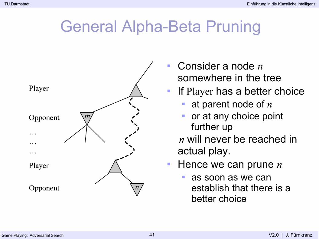
General Alpha-Beta Pruning
Consider a node n somewhere in the tree
If Player has a better choice at parent node of n or at any choice point
further up n will never be reached in
actual play. Hence we can prune n
as soon as we can establish that there is a better choice

Game Playing: Adversarial Search
TU Darmstadt Einführung in die Künstliche Intelligenz
V2.0 | J. Fürnkranz42
Alpha-Cutoff vs. Beta-Cutoff
Graph by Alexander Reinefeld
Of course, cutoffs can also occur at MAX-nodes

Game Playing: Adversarial Search
TU Darmstadt Einführung in die Künstliche Intelligenz
V2.0 | J. Fürnkranz43
Shallow vs. Deep Cutoffs
Graph by Alexander Reinefeld
Cutoffs may occur arbitrarily deep in (sub-)trees

Game Playing: Adversarial Search
TU Darmstadt Einführung in die Künstliche Intelligenz
V2.0 | J. Fürnkranz44
Alpha-Beta Example
0 5 -3 25-2 32-3 033 -501 -350 1-55 3 2-35
Example due to L. Getoor

Game Playing: Adversarial Search
TU Darmstadt Einführung in die Künstliche Intelligenz
V2.0 | J. Fürnkranz45
Alpha-Beta Example
0 5 -3 25-2 32-3 033 -501 -350 1-55 3 2-35
Example due to L. Getoor
[−∞ ,∞]
[−∞ ,∞]
[−∞ ,∞]
[−∞ ,∞]
[−∞ ,∞]
[−∞ ,∞][−∞ , 0]

Game Playing: Adversarial Search
TU Darmstadt Einführung in die Künstliche Intelligenz
V2.0 | J. Fürnkranz46
Alpha-Beta Example
0 5 -3 25-2 32-3 033 -501 -350 1-55 3 2-35
0
0
Example due to L. Getoor
0
[−∞ ,∞]
[−∞ ,∞]
[−∞ ,∞]
[−∞ ,∞]
[−∞ ,∞]
[−∞ ,∞][−∞ ,0 ]

Game Playing: Adversarial Search
TU Darmstadt Einführung in die Künstliche Intelligenz
V2.0 | J. Fürnkranz47
Alpha-Beta Example
0 5 -3 25-2 32-3 033 -501 -350 1-55 3 2-35
0
0 -3
Example due to L. Getoor
0
[−∞ ,∞]
[−∞ ,∞]
[−∞ ,∞]
[−∞ ,∞]
[−∞ ,∞]
[−∞ ,∞]
[−∞ ,∞]
[−∞ ,∞]
[0,∞]
[0,∞]

Game Playing: Adversarial Search
TU Darmstadt Einführung in die Künstliche Intelligenz
V2.0 | J. Fürnkranz48
Alpha-Beta Example
0 5 -3 25-2 32-3 033 -501 -350 1-55 3 2-35
0
0 -3
Example due to L. Getoor
0
[−∞ ,∞]
[−∞ ,∞]
[−∞ ,∞]
[−∞ ,∞]
[0,∞]
[0,∞]

Game Playing: Adversarial Search
TU Darmstadt Einführung in die Künstliche Intelligenz
V2.0 | J. Fürnkranz49
Alpha-Beta Example
0 5 -3 25-2 32-3 033 -501 -350 1-55 3 2-35
0
0
0 -3
Example due to L. Getoor
[−∞ ,∞]
[−∞ ,∞]
[−∞ ,∞]
[−∞ ,∞]
[0,∞]
[0,∞]

Game Playing: Adversarial Search
TU Darmstadt Einführung in die Künstliche Intelligenz
V2.0 | J. Fürnkranz50
Alpha-Beta Example
0 5 -3 25-2 32-3 033 -501 -350 1-55 3 2-35
0
0
0 -3 3
3
Example due to L. Getoor
[−∞ ,∞]
[−∞ ,∞]
[−∞ ,∞]
[−∞ , 0]
[−∞ , 0]
[−∞ , 0]

Game Playing: Adversarial Search
TU Darmstadt Einführung in die Künstliche Intelligenz
V2.0 | J. Fürnkranz51
Alpha-Beta Example
0 5 -3 25-2 32-3 033 -501 -350 1-55 3 2-35
0
0
0 -3 3
3
Example due to L. Getoor
[−∞ ,∞]
[−∞ ,∞]
[−∞ ,∞]
[−∞ ,0]
[−∞ ,0]

Game Playing: Adversarial Search
TU Darmstadt Einführung in die Künstliche Intelligenz
V2.0 | J. Fürnkranz52
Alpha-Beta Example
0 5 -3 25-2 32-3 033 -501 -350 1-55 3 2-35
0
0
0
0 -3 3
3
0
Example due to L. Getoor
[−∞ ,∞]
[−∞ ,∞]
[−∞ ,∞]

Game Playing: Adversarial Search
TU Darmstadt Einführung in die Künstliche Intelligenz
V2.0 | J. Fürnkranz53
Alpha-Beta Example
0 5 -3 25-2 32-3 033 -501 -350 1-55 3 2-35
0
0
0
0 -3 3
3
0
5
Example due to L. Getoor
[−∞ ,∞]
[−∞ ,0 ]
[−∞ ,0 ]
[−∞ ,0 ]
[−∞ , 0]
[−∞ , 0]

Game Playing: Adversarial Search
TU Darmstadt Einführung in die Künstliche Intelligenz
V2.0 | J. Fürnkranz54
Alpha-Beta Example
0 5 -3 25-2 32-3 033 -501 -350 1-55 3 2-35
0
0
0
0 -3 3
3
0
2
2
Example due to L. Getoor
[−∞ ,∞]
[−∞ ,0 ]
[−∞ ,0 ]
[−∞ ,0 ]
[−∞ , 0]
[−∞ , 0]

Game Playing: Adversarial Search
TU Darmstadt Einführung in die Künstliche Intelligenz
V2.0 | J. Fürnkranz55
Alpha-Beta Example
0 5 -3 25-2 32-3 033 -501 -350 1-55 3 2-35
0
0
0
0 -3 3
3
0
2
2
Example due to L. Getoor
[−∞ ,∞]
[−∞ ,0 ]
[−∞ ,0 ]
[−∞ ,0 ]
[−∞ , 0]

Game Playing: Adversarial Search
TU Darmstadt Einführung in die Künstliche Intelligenz
V2.0 | J. Fürnkranz56
Alpha-Beta Example
0 5 -3 25-2 32-3 033 -501 -350 1-55 3 2-35
0
0
0
0 -3 3
3
0
2
2
2
2
Example due to L. Getoor
[−∞ ,∞]
[−∞ ,0 ]
[−∞ ,0 ]
[−∞ ,0 ]

Game Playing: Adversarial Search
TU Darmstadt Einführung in die Künstliche Intelligenz
V2.0 | J. Fürnkranz57
Alpha-Beta Example
0 5 -3 25-2 32-3 033 -501 -350 1-55 3 2-35
0
0
0
0 -3 3
3
0
2
2
2
2
Example due to L. Getoor
[−∞ ,∞]
[−∞ ,0 ]
[−∞ ,0 ]

Game Playing: Adversarial Search
TU Darmstadt Einführung in die Künstliche Intelligenz
V2.0 | J. Fürnkranz58
Alpha-Beta Example
0 5 -3 25-2 32-3 033 -501 -350 1-55 3 2-35
0
0
0
0 -3 3
3
0
2
2
2
2
0
Example due to L. Getoor
[−∞ ,∞]

Game Playing: Adversarial Search
TU Darmstadt Einführung in die Künstliche Intelligenz
V2.0 | J. Fürnkranz59
Alpha-Beta Example
0 5 -3 25-2 32-3 033 -501 -350 1-55 3 2-35
0
0
0
0 -3 3
3
0
2
2
2
2
5
0
Example due to L. Getoor
[0,∞]
[0,∞]
[0,∞]
[0,∞]
[0,∞]
[0,∞]

Game Playing: Adversarial Search
TU Darmstadt Einführung in die Künstliche Intelligenz
V2.0 | J. Fürnkranz60
Alpha-Beta Example
0 5 -3 25-2 32-3 033 -501 -350 1-55 3 2-35
0
0
0
0 -3 3
3
0
2
2
2
2
1
1
0
Example due to L. Getoor
[0,∞]
[0,∞]
[0,∞]
[0,∞]
[0,∞]
[0, 5]

Game Playing: Adversarial Search
TU Darmstadt Einführung in die Künstliche Intelligenz
V2.0 | J. Fürnkranz61
Alpha-Beta Example
0 5 -3 25-2 32-3 033 -501 -350 1-55 3 2-35
0
0
0
0 -3 3
3
0
2
2
2
2
1
1
-3
0
Example due to L. Getoor
[0,∞]
[0,∞]
[0,∞]
[0,∞]
[1,∞]
[1,∞]

Game Playing: Adversarial Search
TU Darmstadt Einführung in die Künstliche Intelligenz
V2.0 | J. Fürnkranz62
Alpha-Beta Example
0 5 -3 25-2 32-3 033 -501 -350 1-55 3 2-35
0
0
0
0 -3 3
3
0
2
2
2
2
1
1
-3
0
Example due to L. Getoor
[0,∞]
[0,∞]
[0,∞]
[0,∞]
[1,∞]
[1,∞]

Game Playing: Adversarial Search
TU Darmstadt Einführung in die Künstliche Intelligenz
V2.0 | J. Fürnkranz63
Alpha-Beta Example
0 5 -3 25-2 32-3 033 -501 -350 1-55 3 2-35
0
0
0
0 -3 3
3
0
2
2
2
2
1
1
-3
1
1
0
Example due to L. Getoor
[0,∞]
[0,∞]
[0,∞]
[0,∞]

Game Playing: Adversarial Search
TU Darmstadt Einführung in die Künstliche Intelligenz
V2.0 | J. Fürnkranz64
Alpha-Beta Example
0 5 -3 25-2 32-3 033 -501 -350 1-55 3 2-35
0
0
0
0 -3 3
3
0
2
2
2
2
1
1
-3
1
1
-5
0
Example due to L. Getoor
[0,∞]
[0,∞]
[1,∞]
[1,∞]
[1,∞]
[1,∞]

Game Playing: Adversarial Search
TU Darmstadt Einführung in die Künstliche Intelligenz
V2.0 | J. Fürnkranz65
Alpha-Beta Example
0 5 -3 25-2 32-3 033 -501 -350 1-55 3 2-35
0
0
0
0 -3 3
3
0
2
2
2
2
1
1
-3
1
1
-5
0
Example due to L. Getoor
[0,∞]
[0,∞]
[1,∞]
[1,∞]
[1,∞]
[1,∞]

Game Playing: Adversarial Search
TU Darmstadt Einführung in die Künstliche Intelligenz
V2.0 | J. Fürnkranz66
Alpha-Beta Example
0 5 -3 25-2 32-3 033 -501 -350 1-55 3 2-35
0
0
0
0 -3 3
3
0
2
2
2
2
1
1
-3
1
1
-5
-5
-5
0
Example due to L. Getoor
[0,∞]
[0,∞]
[1,∞]
[1,∞]
[1,∞]

Game Playing: Adversarial Search
TU Darmstadt Einführung in die Künstliche Intelligenz
V2.0 | J. Fürnkranz67
Alpha-Beta Example
0 5 -3 25-2 32-3 033 -501 -350 1-55 3 2-35
0
0
0
0 -3 3
3
0
2
2
2
2
1
1
-3
1
1
-5
-5
-5
0
1
Example due to L. Getoor
[0,∞]

Game Playing: Adversarial Search
TU Darmstadt Einführung in die Künstliche Intelligenz
V2.0 | J. Fürnkranz68
Alpha-Beta Example
0 5 -3 25-2 32-3 033 -501 -350 1-55 3 2-35
0
0
0
0 -3 3
3
0
2
2
2
2
1
1
-3
1
1
-5
-5
-5
1
1
Example due to L. Getoor
[0,1]
[0,∞]
[0, 1]
[0,1]
[0, 1]
[0,1]
Game Playing: Adversarial Search
TU Darmstadt Einführung in die Künstliche Intelligenz
V2.0 | J. Fürnkranz69
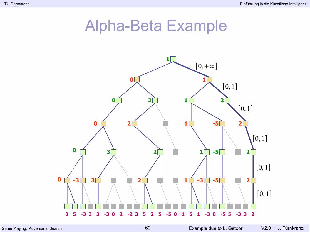
Alpha-Beta Example
0 5 -3 25-2 32-3 033 -501 -350 1-55 3 2-35
0
0
0
0 -3 3
3
0
2
2
2
2
1
1
-3
1
1
-5
-5
-5
1
2
2
2
2
1
Example due to L. Getoor
[0,1]
[0,∞]
[0, 1]
[0,1]
[0, 1]
[0,1]

Game Playing: Adversarial Search
TU Darmstadt Einführung in die Künstliche Intelligenz
V2.0 | J. Fürnkranz70
Alpha-Beta Example
0 5 -3 25-2 32-3 033 -501 -350 1-55 3 2-35
0
0
0
0 -3 3
3
0
2
2
2
2
1
1
-3
1
1
-5
-5
-5
1
2
2
2
2
1
Example due to L. Getoor
Principal VariationThe line that will be played if both players play optimally. The PV determines the value of the position at the root.

Game Playing: Adversarial Search
TU Darmstadt Einführung in die Künstliche Intelligenz
V2.0 | J. Fürnkranz71
Properties of Alpha-Beta Pruning Pruning does not affect final results Entire subtrees can be pruned. Effectiveness depends on ordering of branches
Good move ordering improves effectiveness of pruning With “perfect ordering,” time complexity is O(bm/2)
this corresponds to a branching factor of → Alpha-beta pruning can look twice as deep as minimax in the
same amount of time However, perfect ordering not possible
perfect ordering implies perfect play w/o search random orders have a complexity of O(b3m/4) crude move orders are often possible and get you within a
constant factor of O(bm/2) e.g., in chess: captures and pawn promotions first, forward
moves before backward moves
b

Game Playing: Adversarial Search
TU Darmstadt Einführung in die Künstliche Intelligenz
V2.0 | J. Fürnkranz72
More Information Animated explanations and examples of Alpha-Beta at work
(in German) http://www-i1.informatik.rwth-aachen.de/~algorithmus/algo19.php