turbulent firms, turbulent wages? - harvard … files/09-057.pdf · turbulent firms, turbulent...

Copyright © 2008 by Diego A. Comin, Erica L. Groshen, and Bess Rabin

Working papers are in draft form. This working paper is distributed for purposes of comment and discussion only. It may not be reproduced without permission of the copyright holder. Copies of working papers are available from the author.

Turbulent Firms, Turbulent Wages? Diego A. Comin Erica L. Groshen Bess Rabin

Working Paper

09-057

1

August 15, 2008

Turbulent Firms, Turbulent Wages?

Diego Comin

Harvard Business School and NBER

Erica L. Groshen

Federal Reserve Bank of New York and IZA

and

Bess Rabin

Formerly of the Federal Reserve Bank of New York

We thank Michael Strain for his excellent research assistance and Peter Gottschalk for very useful comments and advice. We also thank participants in the Carnegie-Rochester Conference, HBS and the MaRS/MMS brownbag lunch at the Federal Reserve Bank of New York for their comments and suggestions. The views expressed in this paper are those of the individual authors and do not necessarily reflect the positions of the Federal Reserve Bank of New York or the Federal Reserve System.

2

Turbulent Firms, Turbulent Wages?

Diego Comin

Harvard Business School and NBER

Erica L. Groshen

Federal Reserve Bank of New York

Bess Rabin

Formerly of the Federal Reserve Bank of New York

Abstract

Has greater turbulence among firms fueled rising wage instability in the U.S.? Gottschalk

and Moffitt [1994] find that rising earnings instability was responsible for one third to one half of the rise in wage inequality during the 1980s. These growing transitory fluctuations remain largely unexplained. To help fill this gap, this paper further documents the recent rise in transitory fluctuations in compensation and investigates its linkage to the concurrent rise in volatility of firm performance documented by Comin and Mulani [2006].

We find strong support for the hypothesis that rising high-frequency turbulence in the sales of large publicly-traded U.S. firms over the past three decades has raised their workers’ high-frequency wage volatility. The evidence comes from two data sets: the Panel Study of Income Dynamics (detailed longitudinal information on workers), and COMPUSTAT (detailed firm information, plus average wage and employment levels). Through controls and instrumental variable probes, we rule out straightforward compositional churning as an explanation for the link between firm sales and wage volatility. We also observe that the relationship between sales and wage volatility at the frm level is stronger since 1980, is present only in large companies and is stronger in services than in manufacturing companies.

Keywords: Transitory wage volatility, firm volatility, PSID, turbulence, COMPUSTAT.

JEL: J3, J5.

3

1. Introduction

Has more creative destruction among firms raised wage volatility in the U.S.?

Gottschalk and Moffitt [1994, 2002] called attention to the recent rise in the variation of

transitory earnings for U.S. workers when they estimated that this enhanced volatility

accounts for one third to one half of the rise in wage inequality during the 1980s.1 What is

the source of this new instability in pay? Despite its importance, little is known about its

correlates or origins.2

Most of the related research on the remarkable and well-documented widening of

wage inequality in the U.S. over the past three decades focuses on permanent components

of workers’ earnings, particularly the rising returns to education and ability associated with

technological change, trade, and de-unionization.3 However, this emphasis ignores the less-

studied contribution of larger transitory fluctuations. This study helps to fill that gap.

We conjecture that the recently documented increase in firms’ turbulence has led to

more volatile earnings for their employees. Recent work by Comin and Mulani [2005],

Comin and Philippon [2005] and Davis et al. [2006] finds that the volatility of the

performance of publicly traded firms, whether measured by the profit-to-sales ratio or the

growth rate of sales, employment, or sales per worker, has experienced a prominent upward

trend since at least 1970. They find that the loss of stability at the firm level is due to

heightened creative destruction, stemming from factors including the decline of regulation,

improved capital markets, and more research and development. Hence, the increase in

creative destruction may drive the rise in wage volatility.

Beyond the coincidence of timing, a link between higher firm volatility and the

rising variance of wages is likely on both empirical and theoretical grounds. Empirically,

wage differences among employers for observationally equivalent workers form a

substantial part of wage variation (Groshen [1991a, b], Currie [1992] and Abowd et al.

[2001]), providing a margin on which this effect could operate.

1 Later studies such as Cameron and Tracy [1998] support this finding. Recent work by Autor, Katz and Kearney [2005] also underlines the importance of non-compositional, within-group wage differences in the 1980s and 1990s rise in wage inequality. 2 Violante [2001] posits that returns to skill within firms have become more volatile as the pace of technological change has increased.

4

With regard to theory, there are a wide range of models with relatively rich wage-

setting mechanisms that predict a link between compensation of incumbent workers and

firm performance—in sharp contrast to the perfectly competitive result that workers’ wages

are determined by aggregate, not-firm-specific, conditions. Examples of such richer theories

include the wages that result from bargaining processes between unions and management,

or models with endogenous turnover (e.g. Salop and Salop, 1976).

In these environments, wage premia linked to firm performance will become more

variable as firm performance becomes more volatile. In the canonical example of Nash

bargaining, workers will appropriate part of the firm’s profits in good times delivering an

average wage which is positively correlated to the firm’s performance. In models with

endogenous turnover, firms provide rents to reduce turnover. As a result, a firm will pay

higher wages in periods with a greater marginal hiring cost. In the presence of convex firm

hiring costs, the wage rate will be positively correlated to the firm’s desire to hire workers

which is presumably higher when the firm is performing better. A similar prediction holds

in models where the firm is a monopsonist in the labor market. In these environments, the

wage rate offered to the workers is increasing in the marginal hiring cost which is higher in

good times.

Using the COMPUSTAT data set, which covers the universe of publicly-traded

companies, we explore whether workers’ average pay is more volatile in firms that have

experienced higher turbulence in sales. We find that this is the case, even when we control

for firm characteristics, including average wage, average profits, size, age, or firm-specific

fixed effects.

However, this evidence of a correlation between firm and wage volatility could

reflect reorganization rather than pay changes. That is, if a firm that experienced severe

revenue swings replaced (or laid off) a large part of its workforce, average pay could be

strongly affected even if its continuing workers’ wages were unchanged. To test for this

possibility, we perform a number of tests including controlling for employment growth,

growth in the average wage (to control both for reorganization that affects the number

3 The variance of the permanent component of earnings across workers has increased due to a higher return to education, to a higher return to ability, to globalization, and to institutional changes such as de-unionization. See summaries in Levy and Murnane [1992] and, more recently, Autor, Katz and Kearney [2005]. 5 We have also checked the robustness of our results to using the profit to sales ratio as a measure of the firm performance.

5

and/or the skill/type of workers), and instrumenting firm volatility by lagged firm volatility

and by lagged R&D intensity. All these tests suggest that the linkage between firm and wage

volatility is unlikely to reflect the direct effects of reorganization. Hence, we conclude that

increased firm turbulence has raised the volatility of wages for U.S. workers.

Note that this paper assumes that the direction of causation flows from firm

volatility to earnings volatility, rather than the reverse. We maintain this assumption

because the demand for labor is derived from firms’ product-market demand, rather than

the opposite. Labor supply is typically determined by slow-moving factors such as

population growth, immigration, and education, so we do not think it plausible that a

coincidentally more volatile labor supply is the cause of this phenomenon. To be certain to

control for changes in aggregate supply, we add year dummies and show that the

relationship between wage and firm volatility remains unaffected.

Furthermore, the effect of its own workers’ incomes on a firm’s demand is unlikely

to be a major source of fluctuations in sales for two reasons. First, the share of sales to its

own workers is surely negligible. Second, while more volatile wages could raise the

volatility of workers’ effort (and therefore output and sales), this effect is also unlikely to be

large. Workers’ effort in efficiency wage models depends on the wage relative to the market

wage. Since firm-specific fixed effects explain a substantial fraction of the variation in

wages (Groshen [1991b]), the size of the transitory fluctuations we detect are unlikely to

substantially alter wages relative to the market. Finally, efficiency wage premia are more

likely to be amplification mechanisms than complete theories of fluctuations since they do

not explain why wages fluctuate in the first place.

In the final empirical section, we examine whether the strength of the phenomenon

varies over time or by industrial sector or firm size.. This exercise has several purposes.

First, we explore the consequences for wage volatility of the downward trend in firm

volatility uncovered by Davis et al. (2007) when focusing on non-publicly traded companies.

Since privately-held companies are on average much smaller than publicly-traded companies,

we intend to obtain some understanding of this issue by splitting the COMPUSTAT sample

according to whether firms have more or less than 250 employees. Our findings are striking.

the effect of firm volatility on wage volatility is completely driven by large companies.

These two variables are virtually unrelated for small companies. Based on this finding, we

6

conjecture that the upward trend in individual earnings volatility is much larger for workers

of big publicly-traded companies than for workers of small privately-held companies.

Second, we explore whether the relationship between firm and wage volatility has

changed over time. We find that it has become significantly steeper since 1980. We interpret

this as reflecting the adoption of bonuses in the compensation of workers and the virtual

elimination of piece-wise compensation schemes. This change in compensation practices

may be a consequence of the shift in the composition of jobs towards occupations where

the worker's individual output is harder to monitor. To align the workers and the firm's

incentives the only feasible schemes are those that condition the workers compensation on

the firm's aggregate performance.

Finally, we explore whether there is some cross-sectoral variation in the relationship

between firm and wage volatility. We find that this relationship is steeper in services than in

manufacturing. This finding provides some support to the hypothesis that the increase in

the firm’s risk transferred to workers since 1980 is in part due to the fact that new jobs are

more like ‘service jobs’.

The structure of this paper is as follows. Section 2 describes the data sets and

measures of volatility. Section 3 documents recent trends in volatility in wages and firm

performance in the PSID and COMPUSTAT. Section 4 presents the empirical analysis of

the link between firm performance and wage volatility. Section 5 discusses the results

further, and Section 6 concludes.

2. Measures and Data

Before conducting the empirical analysis we discuss the measures of volatility and

the data we use.

2.1 Measures of volatility

Our analysis focuses on the volatility of three variables:

• log annual earnings of a worker,

• log average wage paid in a firm, and

• log real sales in a firm.5

The first two measure wage turbulence, while the third measures firm turbulence.

We measure the volatility of each variable as the variance over a rolling window of a

7

specified number of years. This measure removes individual or firm-specific averages.

Therefore, its evolution over time controls for major compositional biases. Applied to

wages, this time-series variance captures what Gottschalk and Moffitt (GM) call the

transitory component of wage inequality—the variance in the deviations of a worker’s log

earnings over a given time interval.

The specification of the length of rolling windows is important for volatility analysis.

We choose a length of ten years in order to maintain comparability with the 9-year windows

used by Gottschalk and Moffitt while also preserving the ability to examine the higher

frequency volatility. Formally, our basic measure of the transitory variance for the log of

variable x for cell i in (the interval centered around) year t is defined as follows:

])}[{ln( 4510

+−= t

tilxit xVV τ ,

where V[{.}] denotes the variance of the elements in {.}.

The ten-year transitory variance can be decomposed into two “very transitory”

variances and a “persistent” component. The very transitory variance measures the

fluctuations in the relevant variable over 5-year intervals. This high-frequency volatility is

the main focus of this paper. Formally it is defined as:

])}[{ln( 22

+−= t

tilxit xVV τ

What we call the “persistent” component of transitory variance captures lower

frequency variation and is computed as the variance of two consecutive non-overlapping

five-year averages of the relevant variable. Formally, it is defined as:

]])}[{ln(],)}[{ln([ 415

+−−= t

titti

Plxit xAvgxAvgVV ττ ,

where Avg[{.}] denotes the average of the elements in {.}.

Then, the transitory variance over a 10-year period (close to GM) can be

decomposed into the very transitory variances of the two non-overlapping intervals and the

persistent variance as follows:

V10lxit≡P

lxitlxitlxittti VVVxV ++= +−+− )(2/1])}[{ln( 23

45τ .

To aggregate individual variances across individuals in a given year, we compute the

average of the individual measures of volatility. For firms, we aggregate them by running

weighted regressions on a set of year dummies. As weights we use the share of employment

in the firm in total employment.

8

Starting in 1997, the PSID switched from annual to biennial data collection. As a

consequence, in order to extend the study beyond the early-nineties, we adopt a

methodology which calculates each of the three volatility measures in the interval centered

around year t as the variance of every other year of data. The very transitory volatility in

year t using this “skipping years” methodology, for example, is the variance of the log real

wage in years t-2, t, and t+2. Formally, the very transitory volatility using the skipping years

method for the log of variable x for cell i in year t can be defined as:

])}[{ln( jiS

lxit xVV τ= , j = {t-2, t, t+2).

The calculations using both methodologies are listed in the appendix, and our results are

robust to the type of methodology employed.

2.2 Data

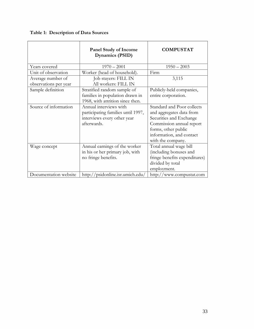
The two data sources we use are compared in Table 1. The Panel Study of Income

Dynamics (PSID) and COMPUSTAT are well-studied, long-lived panels of individual and

firm-level data, respectively. Note that for each wage series we convert to real wages using

the PCE deflator.

The PSID collects annual data for members in a panel of families. As is typical for

wage studies using the PSID, we restrict our sample to heads of households because

information on earnings is most consistent and complete for this group.6 To focus on the

effects of firm volatility on wages for incumbent workers, we also present results for a

sample restricted to job-stayers, workers who have not changed employers over the period.

In the PSID, wages are self-reported earnings from the primary job, divided by hours

worked. Fringe benefits are not included. PSID wage data are very noisy; a high incidence

of error in self-reported earnings and hours generates considerable spurious transitory

variation. However, there is no reason to think that there is any trend in this noise.

COMPUSTAT is compiled by Standard & Poor from annual corporate reports of

publicly traded companies, augmented by other sources as needed. The variables used in

this analysis are annual employment, sales, and wage bill. Employment is the sum of all

workers in the firm including all part-time and seasonal employees, and all employees of

both domestic and foreign consolidated subsidiaries. Our key variable, the wage bill,

9

includes all wage and benefits costs to the company for all employees. We have over 50,000

firm-year observations in COMPUSTAT for the wage bill and between 5 and 6 times more

for employment and sales. These should suffice to explore the trends in firm volatility for

publicly traded companies and the relationship between firm performance volatility and the

volatility of average firm-level wages.

3. Trends in wage and firm volatility

Our first tests of the hypothesis set the stage for the remainder of the study by

documenting the recent rise in wage volatility.

3.1 Individual wage volatility trends in the PSID

This section broadens the evidence on the rise in transitory volatility among

individuals’ earnings by extending the time period and the workers covered and by focusing

on workers who do not change jobs. These extensions form the first tests of our

hypothesis, which predicts that wage volatility continued to rise after 1989, and that this

trend applies to workers who did not change employers and is not restricted to white males.

For comparability with previous studies on firm volatility, we compute volatility measures

using both the log-levels and the growth rates of real earnings. We find that the upward

trend in transitory earnings volatility is quite robust to variants in methodology. The

complete results of these calculations are presented in appendix tables A1, A3, A5, and A7.

Also, Figures 1, 2, and 3 show the plots of the three volatility measures for various groups.

First we repeat the GM exercise in a way as comparable as possible to our analysis

of COMPUSTAT. One adjustment concerns the GM control for age of workers. The

subsequent effects of age on earnings are highly non-linear, so changes in the age structure

of a workforce could alter the volatility of wages even if wage-setting regimes remain

unchanged. To control for changes in the age composition of the sample, GM filter the log

of earnings with a quartic in age prior to computing their volatility measures. Specifically,

GM estimates two quartic regressions, one prior to 1980 and one after 1970. We employ a

6 The head of a household is defined as the husband in a married couple family, a single parent, or an individual who lives alone.

10

similar but more flexible methodology in which we estimate a different age profile for each

year.

An additional adjustment we make is to incorporate demographic weights. Given

the oversampling of poor households and non-random attrition from the program, the

PSID sample is not representative of the U.S. workforce. We correct for these biases by

using the demographic weights provided by the PSID.

Table 3 reports the average transitory volatility of earnings of white male heads of

households in several non-overlapping five-year periods. Table 3a reports results using the

skipping years methodology, while Table 3b reports results using annual data. For brevity,

we will discuss Table 3a; however, the results are robust to the methodology.

The first five rows of Table 3a report the variance of log real annual transitory

earnings over the five non-overlapping periods. The sixth row contains the increment in the

variance of transitory earnings from the first period (1972-1976) to the last period (1995-

1999), and the last row reports the percentage change from the first to the last period.

There are two important observations. First, the volatility of transitory earnings of

white males rose substantially over 10-year periods when extended beyond the GM time

frame. This rise of 5.4 percentage points represents an increase of 67 percent in the

variance of log wages. Second, the rise in transitory earnings volatility for white male heads

of household who did not change employers during the period is similar in magnitude to

the increase for the sample that includes job switchers and represents a larger percent

increase.

Next, we split the 10-year measures shown in Table 3 into their very transitory and

persistent components (as described in the previous section) to determine their separate

influences. For brevity we restrict our attention to measures calculated using the skipping

years methodology.

The first five rows of Table 2a report the average variance of very transitory

earnings in the five non-overlapping 5 year periods. The periods are the same as Table 3a;

the first is 1972-1976 and the fifth is 1995-1999. The average variance of very transitory

real earnings increased by 6 percentage points for white male heads of households and by

4.8 percentage points for white male heads of household who did not change jobs,

representing an increase of 81 and 96 percent, respectively. Table 4a reports the evolution

of the variance of persistent earnings between the same periods. The increment for all

11

white male heads of household is 1.4 percentage points (a 30 percent increase), while for

job-stayers the variance of the persistent component of earnings increased by 0.7

percentage points (a 17 percent increase).

We lose the convenient additive property among the three volatility measures when

we employ the skipping years volatility. However, Tables 2b, 3b, and 4b report the results

using annual data, where the additive property holds. Using these results, we find that both

the very transitory and the more persistent component of earnings changes are important

for explaining the increase in the variance of transitory real earnings. Forty-five to 60

percent of the increase in the variance of transitory real earnings of white males over 10

year periods is due to the increase in the average variance of very transitory earnings, with

the remainder due to increased in variation of the persistent component of real earnings.

For the subgroup who did not change jobs, the share of transitory earnings variance

attributable to the very transitory earnings variance ranges from 35 to 70 percent.

The GM exercise focuses on white males, in contrast to the COMPUSTAT data,

which cover firms and occupations with no demographic limitations. Thus, we extend the

analysis of volatility trends to all heads of households in Tables 2a, 3a, and 4a using the

skipping years methodology. Results are similar using annual data, and are reported in

Tables 2b, 3b, and 4b. We discuss the results using the skipping years method.

Table 2a show that, for all groups, the increase in the variance of very transitory

real earnings is largely monotonic until the last five year period, where it falls slightly. For

workers who did not change jobs, there was a pause in the upward trend of transitory

earnings volatility during the 80s and the trend resumed during the late 80s and early 90s.

Quantitatively, the variance of very transitory earnings rose by 36 percent for all heads of

household and by 46 percent for the subset that did not change jobs.

Table 3a reports the evolution of the variance of the transitory (10-year)

component of earnings for our five year increments. For all heads of households, transitory

volatility rose by 3.2 percentage points, or about 29 percent. For heads who did not change

jobs, transitory volatility rose by 2.7 percentage points, or about 35 percent.

Tables 4a and 4b report the five year increments for the persistent component of

earnings volatility. Using the skipping years methodology, we were able to calculate the

persistent component from 1974 through 1991, and for 1993 and 1995. The change

between the first five year period (1972-1976) and 1995 was 5.9 percent for all heads of

12

households and -5.4 percent for those heads of households who did not change jobs.

However, the percent change from the first period to the mean of the last period for which

we have more than one value (1990-1994) shows an increase of about 25 percent for all

heads and of 8.3 percent for all heads who stayed in their jobs. The result of a positive

increase in the persistent component is also shown using annual data in Table 4b.

We conclude that the rise in the volatility of earnings of individuals persisted into

the 1990s, applies to job-stayers and workers other than white males, and is robust to

various methods of calculation. Furthermore, the very transitory and more persistent

components both play a role in the rise of wage volatility.

3.2 Firm volatility trends in COMPUSTAT

Have transitory variations in firms’ average wages trended up along with other

measures of firm volatility? The affirmative answer to this question provides support for

the hypothesis presented in this paper.

Comin and Mulani [2004] find that the average firm’s sales have become

increasingly volatile in the 50 years since the end of WWII, even as the aggregate economy

has become more stable. More specifically, for each firm in COMPUSTAT, Comin and

Mulani [2004] compute the standard deviation of the firm’s annual growth rate of real sales

over a rolling window. Then the average firm volatility in a year is computed as the average

of the individual firms’ volatilities in a given year.

The upward trend in firm volatility is robust to controlling for mergers and

acquisitions, to weighting the firms’ volatility measures by their share in total sales, to

computing the median firm volatility instead of the average (Comin and Philippon [2005]),

to removing the effect of age and size on the firm volatility measure before aggregating it,

to including firm-specific fixed or cohort effects, and to allowing for size and age-specific

cohort effects (Comin and Mulani [2004]).7 The magnitude of the increment in volatility is

quite robust to almost all of these variations.

Since we cannot present the evolution of the volatility of performance for the firms

in COMPUSTAT for all these variations, we report here two representative aggregation

7 Comin and Mulani [2004] argue that the robustness of the upward trend in volatility to these variations implies that the upward trend in firm volatility is not driven by compositional change in the sample of COMPUSTAT firms.

13

schemes. Aggregation method 1 results from regressing the volatility measure on the log

age -- measured by the years since the firm first appears in COMPUSTAT -- the log of real

sales and a full set of year dummies weighting each observation by the employment in the

firm in the year. The evolution of the volatility measure is given by the coefficients on the

year fixed effects. Aggregation method 2 further controls for compositional change by

including (in addition to the age and size controls) a firm fixed effect. When computing the

effect of firm volatility on wage volatility in section 5, we will use the evolution of firm

from aggregation method 2 since the regressions that estimate the relationship between

firm and wage volatility will include firm-level fixed effects.

Table 5 reports levels of these measures of volatility at the beginning, middle, and

end of the covered period. Panel A reports the measures aggregated according to the first

method (i.e. without firm fixed effects) and Panel B reports the results when aggregated

according to the second (i.e. with firm fixed effects).

Between 1972 and 1999 the very transitory, persistent and transitory variances of

real sales show a steep upward trend. The very transitory volatility of sales computed with

method 1 has increased, respectively, by 7.4 and 6.3 percentage points. Persistent volatility

measures have also increased. In particular, the persistent volatility of real sales increased by

8.3 percentage points between 1974 and 1997. Similarly, the transitory (i.e. over a ten-year

window) volatility of real sales between 1974 and 1997 has increased by 13.5 percentage

points. This steep trend in volatility is completely robust to removing firm heterogeneity

with firm-level fixed effects. If anything, it has become steeper using our second

aggregation scheme. As shown in Panel B of Table 5, the very transitory volatility of sales

increases 21 percentage points while persistent volatility increases by 28 percentage points,

while transitory volatility increases by 43 percentage points, respectively.

COMPUSTAT’s information on the total wage bill of firms allows us to construct a

series of the average wages paid by firms. Table 5 tracks the evolution of the very

transitory, persistent and transitory variances of the firm-level average wage in the

COMPUSTAT sample. The volatility of firms’ average wages has increased. The magnitude

of this increase is smaller than for real sales. This contrast is at least partly due to

respondent bias. Many firms (over 80%) do not report their wage bill in COMPUSTAT,

and those who do report tend to have experienced smaller increases in the volatility of their

sales than non-reporters. Despite this bias, very transitory wage volatility between 1972 and

14

1999 has increased by 1.3 or 2.1 percentage points depending on whether we use

aggregation methods 1 or 2. Persistent wage volatility has increased by less than one

percentage point between 1974 and 1997, and transitory wage volatility has increased by 1.7

or 1.1 percentage points depending on the aggregation method.

Thus, since 1970 both the variance of individual worker real earnings documented

in the PSID and the variance of the average real wages at the firm level in COMPUSTAT

have increased. Applied to the decomposition of the variance of individual earnings in (1),

that means that both the left-hand side term and the first term on the right-hand side have

increased.

3.3 Comparison of trends in firm average wage volatility in COMPUSTAT

with individual wage volatility in the PSID

What fraction of the increase in the variance of individual earnings can be

attributed to the increase in the variance of the average wage paid by firms?

To answer this question, we decompose a worker’s (log) real wage (lwit) as follows:

)( )()( ittiftifit lwlwlwlw −+= ,

where tiflw )( denotes the average wage paid in worker i ’s firm. The second term is the

individual’s idiosyncratic wage change within the firm. Individual wage volatility (Vlwit) is

equal to:

),,(2 )()())(()( tifittiflwittilwftilwflwit lwlwlwCovVVV −++= −

(1)

where the first term in the right-hand side, tilwfV )( , is the variance of the average wage

volatility at the firm level and Cov(x,y) denotes the covariance between x and y. Averaging

across all the individuals, the average individual wage volatility is equal to:

,/// ))(()( ∑∑∑ −+=i

lwittilwfi

tilwfi

lwit NVNVNV

(2)

where the covariance term drops because the two arguments are orthogonal within any

given firm.

15

It follows from (2) that, in order to answer the question posed above, we need to

compute the increment in the volatility of the average wage at the firm level, weighted by

firm employment share.

One important issue in this calculation is whether the increment in the average

weighted firm volatility in COMPUSTAT is an accurate estimate of the increment in the

average weighted firm volatility in the U.S. economy. There are two reasons to be cautious.

First, as argued above, the firms that report the wage bill in COMPUSTAT do not

experience increases in sales volatility as steep as the representative traded firm. We deal

with that by estimating first the relationship between firm volatility and average wage

volatility and then using this elasticity and the evolution of firm volatility in COMPUSTAT

to predict the increment in average wage volatility for the publicly traded companies. A

second reason for caution is the different evolution in the volatility of privately-held

companies (Davis et al. [2007]). We will address this in more detail below by splitting the

COMPUSTAT sample between small (i.e. fewer than 250 employees) and large firms.

Despite those concerns, it is still informative to compare the trend in the volatility

of the average wage paid in the COMPUSTAT firms with the average individual wage

volatility in the PSID. The two samples overlap between 1970 and 2001. Between 1972 and

1999, the very transitory variance of real earnings for workers that did not change jobs in

the PSID has increased by 5.7 percentage points, while between 1974 and 1995, their

persistent variance has not increased and the transitory variance has increased by 3.9

percentage points.

Between 1972 and 1999, the very transitory variance of the firm-level average real

wage in COMPUSTAT aggregated using method 1 increased by 1.4 percentage points,

while using method 2 it increased by 2.1 percentage points. The annual increment in the

very transitory volatility of the average wage paid in the firm is between half and one tenth

of a percentage point.

We can conduct a similar computation to assess the relevance of the evolution of

the between-firm effects in the increment by 2 percentage points in the persistent variance

of individuals’ earnings in the PSID. In particular, the persistent variance of the firm-level

average wage using the first aggregation method has increased by 0.06 percentage points

between 1974 and 1997, while using the second aggregation method it increased by six

tenths of one percentage point.

16

These aggregate time series trends provide some suggestive evidence that, specially,

the increase in very transitory average wage volatility can be an important driver of the

increase in transitory wage inequality documented by Gottschalk and Moffitt [1994]. Next,

we use panel evidence to evaluate more seriously the hypothesis that earnings volatility this

is driven by higher firm instability.

4. Determinants of wage volatility in firms

In this section we explore whether firms that experienced a rise in sales volatility

raised the volatility of the wages they paid to their workers. We first investigate whether

wages are related to firm’s sales using specifications in levels. Second, we turn to

specifications in variances, which allows us to add further controls for omitted variables and

explore the frequency at which relationship holds, After that, we test our hypothesis

separately for measures of very transitory volatility and more,persistent volatility.

4.1 Determinants of firm-level average wage volatility—level regressions

If firm and wage volatility are related because wages respond to firm performance,

we can assess the importance of firm volatility in the increase in earnings volatility by

deriving an elasticity from the estimate of the relationship in levels between sales and

average wages at the firm-level. Though this approach is subject to several caveats that we

describe later, we still find instructive to initiate our exploration showing these results. To

this end we estimate regression (3)

ftftftft Xlslw εγβα +++= , (3)

where lwft denotes the log of the average wage paid in firm f lsft denotes the log of real sales

and Xft is a set of controls that includes the log of the number of employees, year dummies

and may include the log of the age of the firm. The observations are weighted by the

number of employees.

The first two columns of Table 6 report the estimates from this regression. They

show that an increase in real sales of one percentage point is associated with an increase in

the average wage of about 0.73 percent. The second two columns report the results after

including firm fixed effects. These capture persistent differences in average wage across

firms (Groshen, 1991b). Controlling for them does not reduce the association between

17

wages and sales noticeably. The elasticity remains approximately 0.6 and is still highly

significant.

These estimates of β imply that a one percent increase in the variance of real sales is

associated with an increase in the variance of the log average wage of approximately 0.36

percentage points.

This approach to estimating the elasticity between firm and wage volatility has some

limitations compared to regression in variances. First, the economic mechanisms by which

controls should enter in the regression in levels and in variances may be different. For

example, a larger number of employees may allow firms to reduce use of overtime to meet

demand fluctuations and hence may reduce the variability of the average wage per worker.

This effect, however, may not show up on the level regression. Second, in a similar vein, it

may be difficult to control for compositional change in level regressions since we cannot

use changes in levels to control for compositional change. Third, level regressions do not

provide any information about the frequency at which firm and wage volatility are related.

For these reasons the rest of the paper uses regressions in variances.

4.1 Determinants of transitory volatility of firm-level average wages—

variance regressions

We next turn to exploring whether COMPUSTAT firms pay more volatile average

wages when they experience more turbulence. To this end, we estimate the following

regression:

ftftlsftlwft XVV εγβα +++= ,

(4)

where Vlsft is the very transitory variance of sales in firm f between t-2 and t+2, Vlwft is the

variance of log (real wages) in firm f during the same 5 year interval, Xft is a vector of other

controls, and εft is a potentially serially-correlated error term. To obtain an unbiased

estimator of the standard errors of the estimates in the presence of auto-correlated errors,

we use the Newey-West estimator with autocorrelation for up to 5 lags. Regression 3 is run

weighting each observation by their share in total employment. Table 7 reports the

estimates for various specifications.

18

The first column of Table 7 reports the coefficient on sales volatility for the

weighted and unweighted regressions. Very transitory volatility of the average wage paid in

the firm rises strongly and significantly with the very transitory firm volatility of sales.

This positive association persists with the addition of several relevant controls, as

shown in column 2. First, we follow Comin and Mulani [2004] in recognizing that size may

have an effect on firm volatility. Consistent with their findings, we observe that log sales is

negatively related to the variance of the average wage; large firms show less wage volatility.

Second, we also allow for log wage to have an effect on the volatility of wages. This effect is

negative and statistically significant; high-wage firms have less volatile wages. Third, we

control for the log of the firm’s age measured by the years since it first appeared in the

COMPUSTAT sample. We find that younger firms pay more volatile average wages.

However, neither of these latter effects diminishes the coefficient on firm volatility.

The upward trend observed in both sales and wage volatility invites us to add time

trends and year fixed effects to show that the positive association between wage and sales

volatility is not driven by a spurious correlation. Columns 3 and 4 in Table 7 show that the

strength and statistical significance of this association is unaffected by adding a time trend

or time dummies.

One interesting question is whether the observed association between wage and

firm volatility is driven by industry-specific shocks. Columns 5 of Table 7 test this

hypothesis by including 3-digit sector-specific year fixed effects as a control. This does not

reduce the observed relationship between wage and firm volatility.

4.2 Compositional change controls–variance regressions

One important concern, at this point, is whether the observed relationship between

wage and firm volatility is driven by compositional changes that are correlated to firm

performance. There are two forms of potential compositional change that we need to deal

with: across firms and within firms.

Suppose that more volatile firms pay more volatile wages, but when a firm's

performance becomes more volatile the firm does not pay more volatile wages. This

difference between firms would yield positive estimates of β. Further, changes in the

composition of COMPUSTAT towards more volatile firms could produce the observed

upward trends in firm and wage volatility. By contrast, in our hypothesis,,the positive

19

estimate of β results from the within-firm co-movement between wage and employment

volatility, changes in the distribution of aggregate employment across firms should not play

a major role in the increase in wage volatility. That is, the increase in turbulence experienced

by the median firm would drive the increase in transitory wage volatility.

To test whether the positive relation between wage and employment volatility

results from the differences among or within firms, we introduce firm-specific fixed effects

in our regression:

ftftlxftflwft XVtV εγβδα ++++= (5)

Remarkably, introducing firm-specific fixed effects does not affect the significance or size

of the association between firm volatility and the volatility of the average wage at the firm

level (see columns 6 and 7 of Table 7). Thus, we conclude that this association is driven

predominantly by within-firm co-movements between wage and employment volatility and

that the association between wage and firm volatility is driven by within firm dynamics.

A second compositional explanation for the positive association between firm and

wage volatility is that firms which experience more sales turbulence also hire and fire

workers, or open and close establishments, or buy and sell subsidiaries more frequently—

and that, as a result of high job churning, their wage volatility is higher. This explanation is

closely related to Violante [2002] and to Manovski and Kambourov [2004]. However, this

argument faces the problem that the increase in transitory wage volatility (and its

components) in the PSID is the same for those workers that stayed in the same job as for

those who changed jobs during the 5-year period.8 Therefore, it seems likely that the main

force driving the increase in transitory wage volatility operates within the job.

In any case, we would like to assess whether the estimates of β reflect the

association between firm turbulence and the volatility of earnings of individual workers or

firm turbulence and changes in the composition of the workforce in the firm. To explore

the importance of this source of compositional change, we include two additional controls

in regression (5). The first addition is the growth rate of employment over the 5-year

window used to compute the very transitory volatility. This controls for changes in the

composition of employment at the firm level that affect firm size. The second addition is

the growth rate of the average wage in the firm over the 5-year window. This controls for

8 That fact was first noted by Gottschalk and Moffit [1994].

20

changes in the composition of the workforce in the firm that affect the average wage. Such

changes include, for example, changes in the average skill and/or experience of workers.

Columns 8 and 9 in Table 7 report the results from this exercise. As one might

expect, wage volatility is higher in firms that downsize their workforce. This effect, however,

is not significant at standard confidence levels. Similarly, the change in the average wage

over the 5-year interval does not have a significant effect on wage volatility. Interestingly,

controlling for changes in firm size or in the average wage does not affect the magnitude or

significance of the association between wage and firm volatility. The relationship between

wage turbulence and firm turbulence is, thus, unaffected by the controls for compositional

change in the workforce.

4.3 Instrumental variables—variance regressions

Two more alternatives to the hypothesis advanced here for the correlation between

firm and earnings volatility are reverse causality (i.e., higher earnings volatility caused greater

firm instability) and omitted variable bias (i.e., another factor raised both sorts of

turbulence).

As the introduction notes, it is very unlikely that causation runs from wage to firm

volatility for four reasons. First, labor demand is derived from product demand. Second,

the workers in a firm constitute a negligible share of the total demand they face. Third, pure

labor supply fluctuations operate at lower frequencies and, since they are aggregate, are

taken care of by the time dummies. Interestingly, time dummies do not affect the estimated

relationship between firm and wage volatility. A final more interesting channel by which

wage fluctuations may affect firm volatility comes from efficiency wage theory. According

to this theory, fluctuations in the worker’s wage relative to the market wage may affect the

effort exerted by the worker and therefore the firm performance. However, this channel is

unlikely to be important because, given the importance of the firm-level fixed effects in

wages (Groshen [1991b]), the relative position of the firm wages is unlikely to vary much at

the high frequencies studied in this paper.

A second source of concern is omitted variable bias. That is, the positive

association found between firm and earnings volatility could be due to a third omitted

variable that is correlated with both wage and firm volatility and that drives the increase in

the volatility of firm performance and worker’s compensation.

21

We are unaware of any such omitted influence and many of our probes rule out

variants of this alternative hypothesis, so we consider it unlikely. First, the positive

association between firm and wage volatility is robust to the inclusion of firm fixed effects.

Thus, the relationship is not driven by omitted variables that are roughly constant for firms.

This rules out large classes of possible omitted variables, including persistent differences in

compensation schemes across firms that are correlated with their volatility and persistent

cross-sectional variation in the occupational composition of firms.

Similarly, the robustness of our estimates to the inclusion of year fixed effects

implies that the positive association between firm and wage volatility is not driven by

aggregate or regional shocks that affect simultaneously the volatility of wages and firm

performance.

To further discard the possibility that our estimates of β are the result of omitted

variable bias or compositional change we proceed to instrumenting firm volatility. To find

these instruments we borrow from the firm volatility literature, which has identified some

determinants of volatility (Comin and Philippon, 2006, Comin and Mulani, 2007, Comin

and Mulani, 2005). In particular we consider two IVs: lagged volatility and lagged

expenditures in research and development (R&D) at the firm divided by sales. Lagged firm

volatility is correlated with current volatility because there is mean reversion in volatility.

Lagged R&D expenditures predict current volatility because R&D may open new growth

possibilities for the firm. These possibilities may materialize and over a period there may

cause turbulence in the firm performance.

In the first stage, we regress current firm volatility on firm volatility three years ago,

R&D intensity at the firm 4 years ago and the controls we have used in (5). The first two

columns in Table 8 report these results. The difference between these two columns is that

in column 2 we include as an additional control the average profit rate over the 5-year

period over which current volatility is computed. The main observation from the first stage

regression is that the instruments are jointly and individually significant.

A priori, there is no reason why our two instruments should be correlated with the

error term. We do not believe that they should be correlated with average firm performance

over the 5-year volatility window. Nevertheless, we check below for robustness of the

instrumented effect to controlling for the firm’s average profit rate over this period.

22

Similarly, there is no obvious reason why lagged firm volatility or lagged R&D intensity

should affect current wage volatility apart from the effect they have on current volatility.

Instrumented firm volatility has a significant effect on wage volatility in both

specifications, as shown in columns 3 and 4 of Table 8. Interestingly, the magnitude of the

effect of firm volatility on wage volatility (approximately 0.25) is virtually the same as in the

non- instrumented regressions. Given the less than perfect fit in the first stage regression,

one interpretation of this finding is that firm volatility is not endogenous, as the non

instrumented regressions assumed.

4.4 Determinants of persistent volatility of firm-level average wages—

variance regressions

Of course, the relationship between firm and wage volatility may also operate at

lower frequencies. To explore whether this is true we use the measures of persistent

volatility defined above. Specifically, we run the following regression:

.ftftP

lsftP

lwft XVV εγβα +++= (6)

Table 9 reports the estimates of the parameters in equation (5). For brevity we

include from the beginning the baseline set of controls and find in column 1 that there is a

positive association between persistent sales volatility and persistent average wage volatility.

In column 2, we observe that this association is robust to including year fixed effects and to

controlling for the growth rate of sales and employment over the 10-year window over

which persistent volatility is computed. As for the above relationship for transitory volatility,

this shows that the association between wage and firm volatility does not reflect the

omission of changes in the composition of the workforce in the firm. The last column of

Table 9 shows that the association between firm and wage persistent volatility takes place

firms rather than across them.

The first two columns of Table 10 show the robustness of these findings to

instrumenting persistent sales volatility with lagged (5-year) persistent volatility. The strong

mean reversion in persistent volatility (shown in the first column) allows us to use lagged

volatility to obtain variation in current persistent volatility. As with transitory volatility, we

do not believe that the variation induced by lagged persistent volatility is driven by other

variables that affect directly current persistent wage volatility. This is specially the case given

the large set of controls for current state of the firm. (We also experimented with

23

controlling for lagged measures of firm performance and find that the results are robust to

such controls. This provides further proof, in our view, of the exogeneity of the variation

induced by 5-year lagged persistent sales volatility.)

Beyond the statistical significance of the association between wage and sales

persistent volatility, one interesting finding from Tables 9 and 10 is that the magnitude of

this association is approximately one fifth of the size of the association we see between

transitory volatilities. This is not surprising. Even though short-run firm conditions

strongly affect wages paid in firms, in the medium term, firms can adjust along other

margins, so wages tend to be more determined by market (rather than firm) conditions.

5. Accounting for the role of firm turbulence in increased wage turbulence

Next we continue to explore the importance of firm-specific turbulence as an

explanation for higher earnings volatility experienced by workers. In particular, we

investigate whether the slope of the relationship between firm and wage volatility has

changed over time, and whether it varies by firm size and by sector. We conclude by taking

stock of our findings and computing the increment in earnings volatility due to firm specific

factors.

5.1 Changes in the slope?

Have firms increased the loading of their workers in the firm performance recently?

To explore this possibility, we re-estimate our regressions splitting the dataset in two

samples, before and after 1980. The first two columns of Table 11 report the results from

estimating these two regressions for the instrumented very transitory volatility measures.

The results are striking. The coefficient before 1980 was an insignificant 4 percent, while

after 1980 it was a significant 26 percent. So, the effect of very transitory firm volatility on

very transitory wage volatility seems to be a phenomenon that virtually started in the 80s.

Columns 3 and 4 of Table 10 show, however, that there has been no significant increase in

the effect of persistent firm volatility on persistent wage volatility.

Why have firms adopted compensation schemes that are more loaded on firm

performance? Answering this question goes beyond the scope of this paper but we feel

compelled to speculate. One possibility is that the new jobs created as a result of the

24

adoption of computers and the expansion of the service economy are harder to monitor.

Hence, it was not possible to condition the worker on his individual performance to align

the workers’ incentives with firm goals,. The second best option is to condition the

compensation of the only observable, that is, firm performance.

The latter part of the 20th century saw a decline in the prevalence of piece-rate

compensation, while bonuses have become much more common (Milcovich and Stevens

1999; Levine et al. 2002). We shall show below some more quantitative evidence in support

of this story when exploring the sectoral variation in the relationship between firm and

wage volatility.

In another story, factors such as declining unionism and real value of the minimum

wage in the US (Freeman 2008), have led some observers (Gali and This, 2008) to argue

that US labor markets have moved closer to a spot market since around 1980, and away

from arrangements where firms sheltered workers from aggregate fluctuations. Note that

this hypothesis, would not deliver a priori the findings of this paper because movement

toward a spot labor market would weaken the connection between firm volatility and wage

volatility rather than strengthen it, as has occurred in the US publicly traded companies

since 1980.

5.2 Differences between large and small firms

Do we observe any variation in the relationship between firm and wage volatility

across firm size? To answer this question we re-estimate our baseline regressions splitting

the COMPUSTAT sample into large and small firms, using 250 employees as the threshold.

Since COMPUSTAT over-represents large companies the subsample of over 250

employees will be much larger than the subsample of less than 250 employees, but we will

still be able to compare the point estimates.

Columns 3 and 4 of Table 11 report the estimates for the instrumented transitory

volatility measures. We find a sharp contrast in the effects of transitory firm volatility on

wage volatility for big and for small firms. While for big firms there is a significant effect

(comparable to the effect reported in the previous analysis), for small firms there is virtually

no effect of firm volatility on wage volatility. Given the small subsample of small firms we

also report in columns 5 and 6 the results for regressions where firm volatility is not

instrumented. These are basically the same as those for the instrumented regressions.

25

Columns 5 and 6 of Table 10 show that there is no significant difference in the effect of

persistent firm volatility on the persistent volatility of wages between big and small firms.

These findings are significant in the light of the conclusion reached by Davis et al.

(2007) that privately-held firms have become less volatile since the mid 1970s. Since

privately-held companies are much smaller than publicly-traded ones, it seems reasonable to

think of the relationship between firm and wage volatility for privately-held firms as similar

to the relationship found in COMPUSTAT for small firms. Hence, the picture that emerges

is that large companies became more volatile and found it optimal to pass along some of

this greater turbulence to their employees in the form of more volatile earnings. Small firms

may have experienced a decline in volatility, but, since they have not found it optimal to

link their wages so tightly to firm performance, their employees’ wages have not become

more stable.

Why have only large companies passed on their turbulence to their workers in the

form of more volatile wages? This finding may seem surprising at first. According to agency

theories of compensation (e.g., Holmstrom, 1982), the optimal compensation of a worker

has a loading of b>0 in the worker’s signal and a loading of d on the firm’s signal, with

0>d>-b,. For larger firms, the firm-level signal is less noisy and therefore the loading d

becomes closer to –b, reducing the dependence of the average wage in the company on the

firm’s performance.

A more promising avenue of future research may reside in thinking of big firms as

monpsonists in the labor markets where they operate. In such environments it may be

possible to write models where the wages these firms pay vary with the product demand

conditions they experience. Small firms, in contrast, are price takers in the labor markets.

Therefore, the wages they pay do not vary with firm conditions but are determined by

aggregate factors.

5.3 Differences across sectors

Finally, we explore whether the link between sales volatility and wage volatility at

the firm level is stronger or weaker in manufacturing than in non-manufacturing sectors.

Columns 7 and 8 of Table 11 report the estimates for both sub-samples after instrumenting

very transitory volatility and columns 9 and 10 report the estimates without instrumentation.

The main finding is that the slope of the relationship between firm and wage volatility is

26

steeper in non-manufacturing firms than in manufacturing firms. The slope is not

significant in the non-manufacturing sub-sample due to the reduction in the sample size

due to the use of R&D intensity as instrument. The point estimate, however is very large

(0.58). When we do not instrument we find a significantly larger estimate in the non-

manufacturing sub-sample.

As advanced above, the larger effect of firm volatility on wage volatility found in

non-manufacturing provides some support to the notion that part of the increase in the

coefficient observed since 1980 may be driven by the difficulty to condition the workers’

compensation on their own performance inherent in many jobs in the service sector. New

jobs created due to the digital revolution are more service-like in their difficulty to observe

easily the individual performance of a worker and hence the need to condition of firm-level

performance measures to align the incentives of the workers and the company.

5.4 Adding up

How much of the increment in earnings volatility can be traced back to firm

volatility? To answer this question we offer first a simple calculation based on regressions 5

and 6. Given an estimate for β of 0.25 for the very transitory volatility regressions, and an

increment in the very transitory volatility of real sales of 0.21, the increment in the very

transitory volatility of average earnings induced by the higher very transitory volatility

experienced by firms is of 5.2 percentage points. As shown in the second row of Table 12,

an equivalent calculation shows that 1.1 percentage points of the persistent volatility of the

average wage at the firm level are driven by the increment in the persistent volatility of firm-

level sales. Hence, the increment in transitory firm volatility (i.e., the sum of very transitory

and persistent) has lead to an increase in 6.3 percentage points for the transitory volatility of

the earnings of publicly-traded companies.

But this is just part of the story. As firms have increased the leverage of the workers

compensation on the firm’s performance, firm turbulence has also been increased earnings

volatility. Using the estimates of the increment of β from Tables 10 and 11, rows 3 and 4 of

Table 12 compute the additional effect that this has on the increment in the volatility of the

average wage at very transitory and persistent frequencies.

Very transitory volatility of the average wage rate at the firm level increases by 1.2

additional percentage points. While, given the lack of a significant increment in the slope of

27

the relationship between persistent volatility measures, the computation of the increment in

persistent wage volatility does not change.

Adding up, we find that the transitory volatility of the average firm level wages of

workers in publicly-traded companies has increased by 7.5 percentage points between 1970

and 1999 due to the turbulence experienced by their firms. This figure is approximately 2.5

times higher than the observed increment in transitory volatility during the same period in

the PSID (2.7 percentage points). It is, of course, perfectly plausible that our predicted

increase is higher than the observed increase in the PSID. This is the case because

COMPUSTAT only covers publicly-traded companies and our best guess for the evolution

of the average wage in the non-publicly traded companies based on the smaller companies

in COMPUSTAT is that it has not increased. Hence, firm turbulence seems an important

factor towards understanding the evolution of individual workers’ earnings volatility.

6. Conclusion

Our findings suggest that rising turbulence in sales among U.S. firms over the past

three decades has raised their workers’ wage volatility, increasing wage risks for many

workers. The effect is strong and has grown markedly since the 1980s.

Using household panel data in the PSID, GM find that wage volatility has risen

substantially for white male workers. We confirm the robustness of this result, focusing on

workers who have not changed jobs and extending it to all demographic groups. Using

firm data from COMPUSTAT, we find rising volatility of firms’ mean wages that mirrors

the rise in volatility of firm performance and robust evidence that when firms experience

more turbulence they pay more volatile wages.

To ensure that the connection between these two volatilities does not reflect the

impact of the impact of compositional changes between or within firms, we turn to

additional controls and instrumental variables. The positive impact of firm turbulence on

wage volatility is robust to the introduction of these controls both for volatility measures

that capture very transitory and more persistent changes.

Our analysis focuses on the impact of this turbulence on wage changes for

incumbent workers, not for workers who have changed jobs. However, there are reasons

to think that the increase in firm turbulence may also increase risk for workers who switch

28

employers. First, firm turbulence may increase the dispersion of average wages in

occupations within a firm or in a given occupation across firms. Second, because of these

two forces, firm turbulence may lead to more job turnover. We leave exploration of these

hypotheses for future work.

Our findings have important implications for theories of labor markets and optimal

wage compensation schemes. Existing models cannot explain all the findings uncovered in

this paper. Perfectly competitive labor market models cannot explain the effect of firm

volatility on wage volatility. Models of compensation based on agency theory cannot

explain the observed larger effect of firm volatility on wage volatility in large than small

companies. Finally, models of de-unionization cannot account for the increase in the link

between firm and wage volatility observed since 1980.

Finally, from a policy standpoint, these findings highlight a source of increased risk

faced by U.S. workers since the 1980s. As they adjust to the decline of defined-benefit

pensions, health insurance, social safety net programs, and job security, Americans now find

their paychecks tied to increasingly rocky corporate ships. The implications of this

heightened risk for financial markets and for social and economic policy, not to mention

families and communities, are still unknown.

29

References

Abowd, John, Francis Kramarz, David N. Margolis, and Kenneth R. Troske, 2001. “The Relative Importance of Employer and Employee Effects on Compensation: A Comparison of France and the United States.” Journal of the Japanese and International Economies.

Abowd, John A. and Thomas Lemieux, 1993. “The Effects of Product Market Competition on Collective Bargaining Agreements: The Case of Foreign Competition in Canada.” Quarterly Journal of Economics 108: 983-1014.

Autor, David H., Lawrence F. Katz, and Melissa S. Kearney. 2005. “Rising Wage Inequality: the Role of Composition and Prices.” MIT unpublished paper.

Cameron, Stephen and Joseph Tracy. 1998. “Earnings Variability in the United States; An Examination Using Matched-CPS Data.” Unpublished paper, Federal Reserve Bank of New York: October.

Comin, Diego and Sunil Mulani,. 2004. “Diverging Trends in Macro and Micro Volatility: Facts,” Forthcoming Review of Economics and Statistics.

Comin, Diego and Sunil Mulani. 2005. “A Theory of Growth and Volatility at the Aggregate and Firm Level.” NBER Working Paper 11503, June.

Comin, Diego and Thomas Philippon. 2005. “The Rise in Firm-Level Volatility: Causes and Consequences.” NBER Macroeconomics Annual Vol. 20. Eds. Mark Gertler and Kenneth Rogoff. Cambridge, MA.

Currie, Janet and Sheena McConnell, 1992. “Firm-Specific Determinants of the Real Wage.” Review of Economics and Statistics, 74 (2): 297-304.

Davis, Steve, John Haltiwanger, Ron Jarmin, and Javier Miranda. 2007. “Volatility and dispersion in Business Growth Rates: Publicly Traded Versus Privately Held Firms” NBER Macroeconomics Annual, Vol. 21. Eds. Daron Acemoglu, Kenneth Rogoff, and Michael Woodford. Cambridge, MA.

Freeman, Richard. 2008. “Labor Market Institutions Around the World,” London School of Economics, Centre for Economic Performance Discussion Paper #0844.

Gertler, Mark and Simon Gilchrist. 1994. “Monetary Policy, Business Cycles and the

Behavior of Small Manufacturing Firms.” Quarterly Journal of Economics, 109, May, 309-340.

Gottschalk, Peter and Robert Moffit. 2002. "Trends in the Transitory Variance of Earnings in the U.S." The Economic Journal, 112 (478), C68-C73.

Gottschalk, Peter, and Robert Moffitt. 1994. “The Growth of Earnings Instability in the U.S. Labor Market.” Brookings Papers on Economic Activity 2: 217-272.

30

Groshen, Erica L. 1996. “American Employer Salary Surveys and Labor Economics Research: Issues and Contributions,” Annales d’Economie et de Statistique 41/42: 413-442.

Groshen, Erica L. 1991a. “Five Reasons Why Wages Vary Among Employers.” Industrial Relations 30: 350-381.

Groshen, Erica L. 1991b. “Sources of Intra-Industry Wage Dispersion: How Much Do Employers Matter?” Quarterly Journal of Economics, 106: 869-884.

Groshen, Erica L. “Do Wage Differences Among Employers Last?” Federal Reserve Bank of Cleveland Working Paper No. 8906, 1989 [revised 1991].

Juhn, Chinhui, Kevin M. Murphy and Brooks Pierce. 1993. “Wage Inequality and the Rise in the Returns to Skill.” Journal of Political Economy 101 (3): 410-442.

Kremer, Michael and Eric Maskin. 1995. “Wage Inequality and Segregation by Skill.” NBER Working Paper 5718.

Levine, David I., Dale Belman, Gary Charness, Erica L. Groshen, and K.C. O’Shaughnessy. 2002. How New is the New Employment Contract? Evidence from North American Pay Practices. WE Upjohn for Employment Research Press: Kalamazoo, MI.

Levy, Frank and Richard J. Murnane. 1992. “U.S. Earnings Levels and Earnings Inequality: A Review of Recent Trends and Proposed Explanations,” Journal Economic Literature. 30 (3): 1333-1381.

Manovskii, Iourii, and Gueorgui Kambourov. 2004. “Occupational Mobility and Wage Inequality.” mimeo University of Pennsylvania.

Milkovich, George and Jennifer Stevens. 1999. “Back to the Future: A Century of Compensation,” Industrial and Labor Relations School, Cornell University, Center for Advanced Human Resource Studies Working Paper 99-08.

Violante, Gianluca. 2002. “Technological Acceleration, Skill Transferability and the Rise in Residual Wage Inequality.” Quarterly Journal of Economics, 117: 297-338.

31

PSID Appendix – Construction of Samples

This document details the steps used to construct the dataset we use to analyze the transitory and persistent volatility of wages.

1. The first thing we do is download the data from the PSID family file. All wage data come from the family file except for the years 1994 through 2001, which come from the Income Plus file. Demographic data are downloaded in order to generate our sample. Weights are also downloaded.

2. The data are all “wide.” In other words, each row in the matrix corresponds to the head of the household, and the columns are that head’s 1970 PSID code, his 1970 wage, his 1971 code, his 1971 wage,…, his 2001 code, his 2001 wage. We now go through each dataset (wage file, sex file, age file, etc.) and drop the blank code observations. This ensures that all individuals have a PSID code for each year.

3. At this point we merge the various datasets into one master dataset. In other words, we merge wage data, age data, sex data, the weights, a price index, etc. into a master file. The price index we use is the monthly personal consumption expenditures chain-type price index, aggregated to annual values, with 1982 equal to zero.

4. We now use the wage data to compute the natural log of the real wage.

5. We apply an age filter to the log real wage. To do this, we regress log real wage on a quartic in age and collect the residuals, which we call the age filtered log real wage.

For analysis of all heads:

6. At this point we begin to generate our sample. We drop heads who are greater than sixty or less than nineteen years of age.

7. We drop all heads who are full time students.

8. We replace all observations with a wage equal to zero as a missing value.

9. After this, we drop all heads who report income of less than or equal to the first percentile and greater than or equal to the ninety-ninth percentile. After this step is taken, there are no observations which remain with a topcoded value as their wage.

10. At this point we reshape the data as “long” and are able to compute our volatility measures. The five and ten year volatility measures are only computed for individuals with five and ten years of consecutive non-zero wage data, respectively.

32

For analysis of white male heads:

6. At this point we begin to generate our sample. We drop all heads who are not male.

7. We drop all heads who are not white.

8. We drop heads who are greater than sixty or less than nineteen years of age.

9. We drop all heads who are full time students.

10. We replace all observations with a wage equal to zero as a missing value.

11. After this, we drop all heads who report income of less than or equal to the first percentile and greater than or equal to the ninety-ninth percentile. After this step is taken, there are no observations which remain with a topcoded value as their wage.

12. At this point we reshape the data as “long” and are able to compute our volatility measures. The five and ten year volatility measures are only computed for individuals with five and ten years of consecutive non-zero wage data, respectively.

33

Table 1: Description of Data Sources

Panel Study of Income

Dynamics (PSID)

COMPUSTAT

Years covered 1970 – 2001 1950 – 2003 Unit of observation Worker (head of household). Firm Average number of observations per year

Job stayers: FILL IN All workers: FILL IN

3,115

Sample definition Stratified random sample of families in population drawn in 1968, with attrition since then.

Publicly-held companies, entire corporation.

Source of information Annual interviews with participating families until 1997, interviews every other year afterwards.

Standard and Poor collects and aggregates data from Securities and Exchange Commission annual report forms, other public information, and contact with the company.

Wage concept Annual earnings of the worker in his or her primary job, with no fringe benefits.

Total annual wage bill (including bonuses and fringe benefits expenditures) divided by total employment.

Documentation website http://psidonline.isr.umich.edu/ http://www.compustat.com

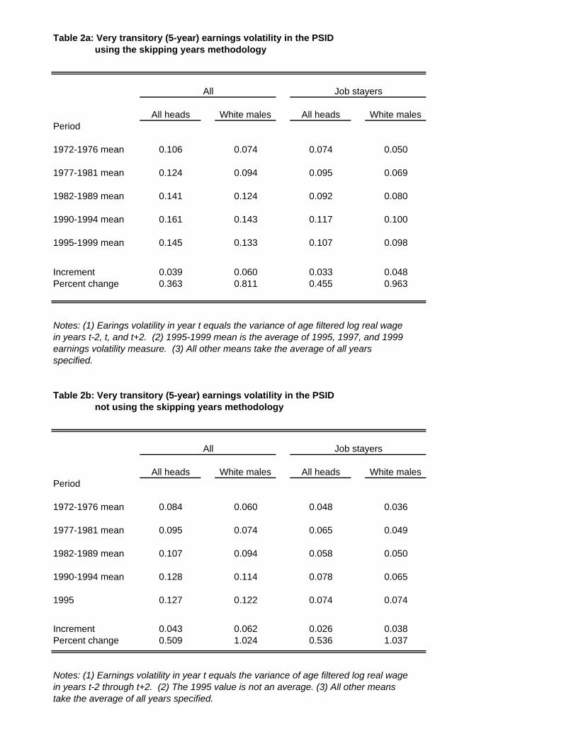
Table 2a: Very transitory (5-year) earnings volatility in the PSID using the skipping years methodology

All heads White males All heads White malesPeriod

1972-1976 mean 0.106 0.074 0.074 0.050

1977-1981 mean 0.124 0.094 0.095 0.069

1982-1989 mean 0.141 0.124 0.092 0.080

1990-1994 mean 0.161 0.143 0.117 0.100

1995-1999 mean 0.145 0.133 0.107 0.098

Increment 0.039 0.060 0.033 0.048Percent change 0.363 0.811 0.455 0.963

Notes: (1) Earings volatility in year t equals the variance of age filtered log real wagein years t-2, t, and t+2. (2) 1995-1999 mean is the average of 1995, 1997, and 1999earnings volatility measure. (3) All other means take the average of all years specified.

Table 2b: Very transitory (5-year) earnings volatility in the PSID not using the skipping years methodology


1972-1976 mean 0.084 0.060 0.048 0.036

1977-1981 mean 0.095 0.074 0.065 0.049

1982-1989 mean 0.107 0.094 0.058 0.050

1990-1994 mean 0.128 0.114 0.078 0.065

1995 0.127 0.122 0.074 0.074


Notes: (1) Earnings volatility in year t equals the variance of age filtered log real wagein years t-2 through t+2. (2) The 1995 value is not an average. (3) All other means take the average of all years specified.

All Job stayers

All Job stayers

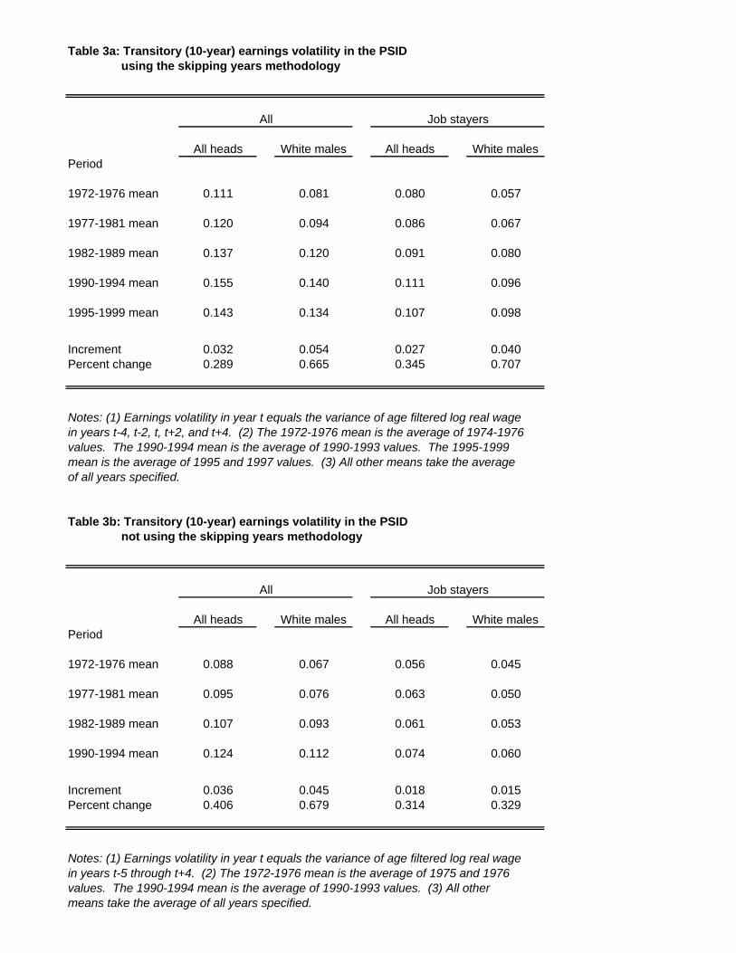
Table 3a: Transitory (10-year) earnings volatility in the PSID using the skipping years methodology


1972-1976 mean 0.111 0.081 0.080 0.057

1977-1981 mean 0.120 0.094 0.086 0.067

1982-1989 mean 0.137 0.120 0.091 0.080

1990-1994 mean 0.155 0.140 0.111 0.096

1995-1999 mean 0.143 0.134 0.107 0.098


Notes: (1) Earnings volatility in year t equals the variance of age filtered log real wage in years t-4, t-2, t, t+2, and t+4. (2) The 1972-1976 mean is the average of 1974-1976 values. The 1990-1994 mean is the average of 1990-1993 values. The 1995-1999 mean is the average of 1995 and 1997 values. (3) All other means take the average of all years specified.

Table 3b: Transitory (10-year) earnings volatility in the PSID not using the skipping years methodology


1972-1976 mean 0.088 0.067 0.056 0.045

1977-1981 mean 0.095 0.076 0.063 0.050

1982-1989 mean 0.107 0.093 0.061 0.053

1990-1994 mean 0.124 0.112 0.074 0.060


Notes: (1) Earnings volatility in year t equals the variance of age filtered log real wage in years t-5 through t+4. (2) The 1972-1976 mean is the average of 1975 and 1976 values. The 1990-1994 mean is the average of 1990-1993 values. (3) All other means take the average of all years specified.

All Job stayers

All Job stayers

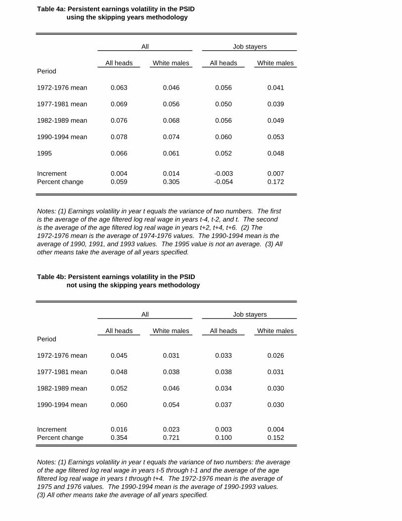
Table 4a: Persistent earnings volatility in the PSID using the skipping years methodology


1972-1976 mean 0.063 0.046 0.056 0.041

1977-1981 mean 0.069 0.056 0.050 0.039

1982-1989 mean 0.076 0.068 0.056 0.049

1990-1994 mean 0.078 0.074 0.060 0.053

1995 0.066 0.061 0.052 0.048

Increment 0.004 0.014 -0.003 0.007Percent change 0.059 0.305 -0.054 0.172

Notes: (1) Earnings volatility in year t equals the variance of two numbers. The first is the average of the age filtered log real wage in years t-4, t-2, and t. The second is the average of the age filtered log real wage in years t+2, t+4, t+6. (2) The1972-1976 mean is the average of 1974-1976 values. The 1990-1994 mean is theaverage of 1990, 1991, and 1993 values. The 1995 value is not an average. (3) All other means take the average of all years specified.

Table 4b: Persistent earnings volatility in the PSID not using the skipping years methodology


1972-1976 mean 0.045 0.031 0.033 0.026

1977-1981 mean 0.048 0.038 0.038 0.031

1982-1989 mean 0.052 0.046 0.034 0.030

1990-1994 mean 0.060 0.054 0.037 0.030


Notes: (1) Earnings volatility in year t equals the variance of two numbers: the average of the age filtered log real wage in years t-5 through t-1 and the average of the age filtered log real wage in years t through t+4. The 1972-1976 mean is the average of 1975 and 1976 values. The 1990-1994 mean is the average of 1990-1993 values. (3) All other means take the average of all years specified.

All Job stayers

All Job stayers

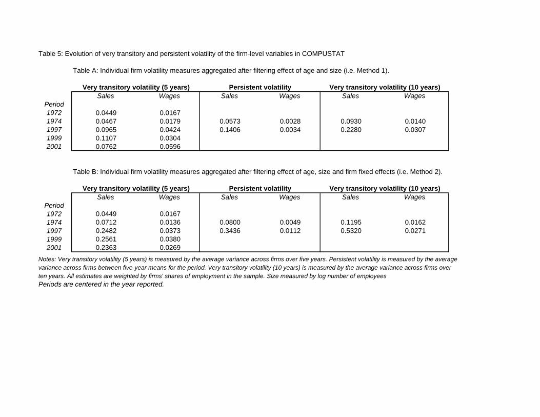
Table 5: Evolution of very transitory and persistent volatility of the firm-level variables in COMPUSTAT

Table A: Individual firm volatility measures aggregated after filtering effect of age and size (i.e. Method 1).

Sales Wages Sales Wages Sales WagesPeriod1972 0.0449 0.0167 1974 0.0467 0.0179 0.0573 0.0028 0.0930 0.01401997 0.0965 0.0424 0.1406 0.0034 0.2280 0.03071999 0.1107 0.0304 2001 0.0762 0.0596

Table B: Individual firm volatility measures aggregated after filtering effect of age, size and firm fixed effects (i.e. Method 2).

Sales Wages Sales Wages Sales WagesPeriod1972 0.0449 0.0167 1974 0.0712 0.0136 0.0800 0.0049 0.1195 0.01621997 0.2482 0.0373 0.3436 0.0112 0.5320 0.02711999 0.2561 0.0380 2001 0.2363 0.0269

Notes: Very transitory volatility (5 years) is measured by the average variance across firms over five years. Persistent volatility is measured by the average variance across firms between five-year means for the period. Very transitory volatility (10 years) is measured by the average variance across firms over ten years. All estimates are weighted by firms' shares of employment in the sample. Size measured by log number of employeesPeriods are centered in the year reported.

Persistent volatility Very transitory volatility (10 years)

Very transitory volatility (5 years) Persistent volatility Very transitory volatility (10 years)

Very transitory volatility (5 years)

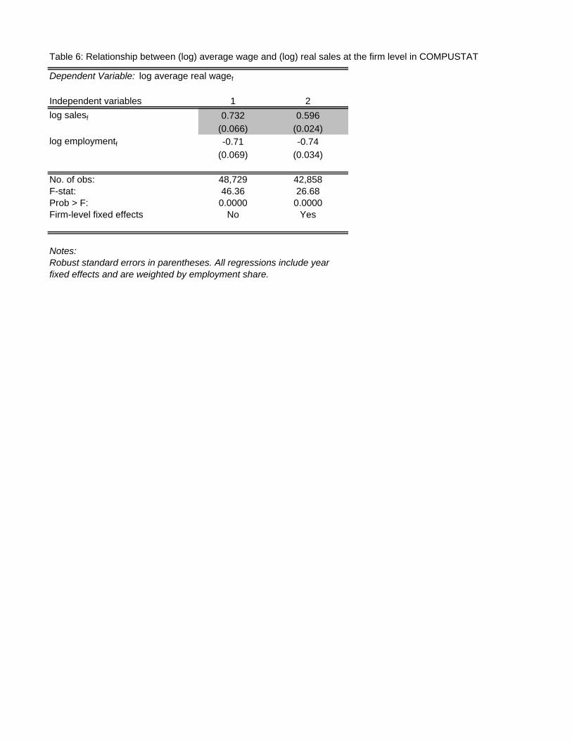
Table 6: Relationship between (log) average wage and (log) real sales at the firm level in COMPUSTAT

Dependent Variable: log average real wagef

Independent variables 1 2log salesf 0.732 0.596

(0.066) (0.024)log employmentf -0.71 -0.74

(0.069) (0.034)

No. of obs: 48,729 42,858F-stat: 46.36 26.68Prob > F: 0.0000 0.0000Firm-level fixed effects No Yes

Notes:

fixed effects and are weighted by employment share. Robust standard errors in parentheses. All regressions include year

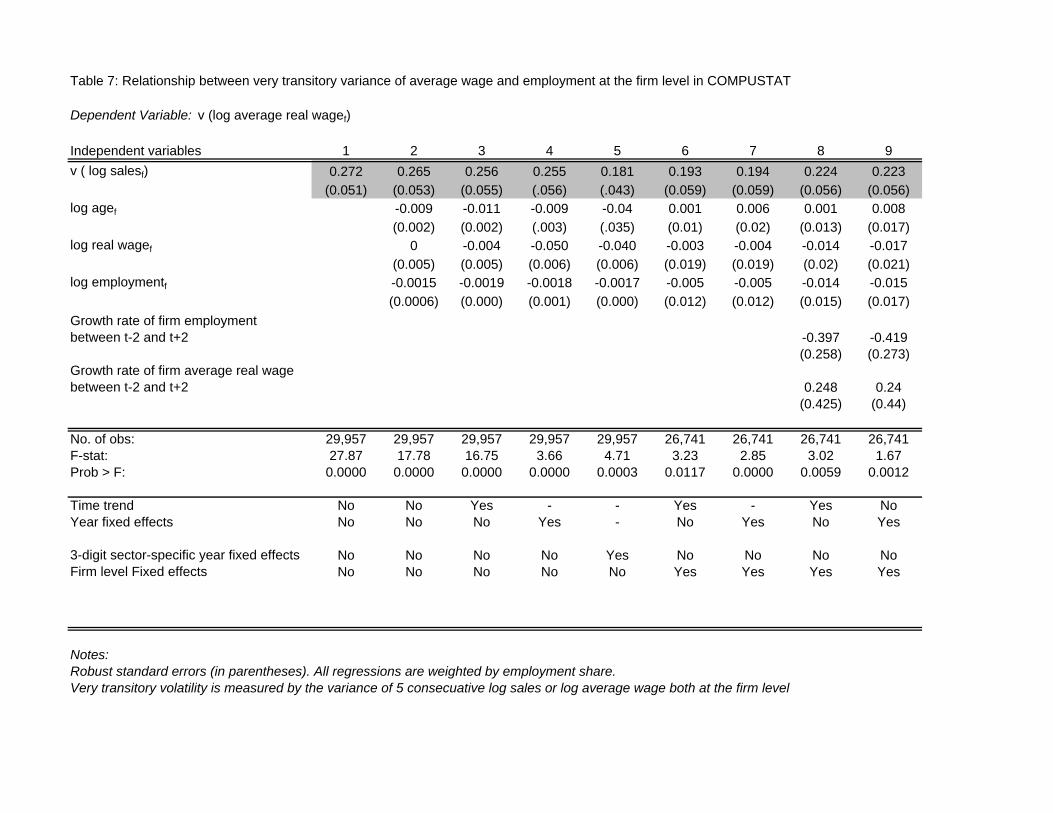
Table 7: Relationship between very transitory variance of average wage and employment at the firm level in COMPUSTAT

Dependent Variable: v (log average real wagef)

Independent variables 1 2 3 4 5 6 7 8 9v ( log salesf) 0.272 0.265 0.256 0.255 0.181 0.193 0.194 0.224 0.223

(0.051) (0.053) (0.055) (.056) (.043) (0.059) (0.059) (0.056) (0.056)log agef -0.009 -0.011 -0.009 -0.04 0.001 0.006 0.001 0.008

(0.002) (0.002) (.003) (.035) (0.01) (0.02) (0.013) (0.017)log real wagef 0 -0.004 -0.050 -0.040 -0.003 -0.004 -0.014 -0.017

(0.005) (0.005) (0.006) (0.006) (0.019) (0.019) (0.02) (0.021)log employmentf -0.0015 -0.0019 -0.0018 -0.0017 -0.005 -0.005 -0.014 -0.015

(0.0006) (0.000) (0.001) (0.000) (0.012) (0.012) (0.015) (0.017)Growth rate of firm employment between t-2 and t+2 -0.397 -0.419

(0.258) (0.273)Growth rate of firm average real wage between t-2 and t+2 0.248 0.24

(0.425) (0.44)

No. of obs: 29,957 29,957 29,957 29,957 29,957 26,741 26,741 26,741 26,741F-stat: 27.87 17.78 16.75 3.66 4.71 3.23 2.85 3.02 1.67Prob > F: 0.0000 0.0000 0.0000 0.0000 0.0003 0.0117 0.0000 0.0059 0.0012

Time trend No No Yes - - Yes - Yes NoYear fixed effects No No No Yes - No Yes No Yes

3-digit sector-specific year fixed effects No No No No Yes No No No NoFirm level Fixed effects No No No No No Yes Yes Yes Yes

Notes:

Very transitory volatility is measured by the variance of 5 consecuative log sales or log average wage both at the firm levelRobust standard errors (in parentheses). All regressions are weighted by employment share.

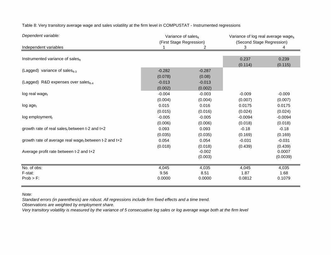
Table 8: Very transitory average wage and sales volatility at the firm level in COMPUSTAT - Instrumented regressions

Dependent variable:

Independent variables 1 2 3 4 Instrumented variance of salesft 0.237 0.239

(0.114) (0.115)(Lagged) variance of salesft-3 -0.282 -0.287

(0.078) (0.08)(Lagged) R&D expenses over salesft-4 -0.013 -0.013

(0.002) (0.002)log real wagef -0.004 -0.003 -0.009 -0.009

(0.004) (0.004) (0.007) (0.007)log agef 0.015 0.016 0.0175 0.0175

(0.015) (0.016) (0.024) (0.024)log employmentf -0.005 -0.005 -0.0094 -0.0094

(0.006) (0.006) (0.018) (0.018)growth rate of real salesf between t-2 and t+2 0.093 0.093 -0.18 -0.18

(0.035) (0.035) (0.169) (0.169)growth rate of average real wagef between t-2 and t+2 0.054 0.054 -0.031 -0.031

(0.018) (0.018) (0.439) (0.439)Average profit rate between t-2 and t+2 -0.002 0.0007

(0.003) (0.0039)

No. of obs: 4,045 4,035 4,045 4,035F-stat: 9.56 8.51 1.87 1.68Prob > F: 0.0000 0.0000 0.0812 0.1079

Observations are weighted by employment share. Very transitory volatility is measured by the variance of 5 consecuative log sales or log average wage both at the firm level

Note: Standard errors (in parenthesis) are robust. All regressions include firm fixed effects and a time trend.

Variance of log real average wageftVariance of salesft

(First Stage Regression) (Second Stage Regression)

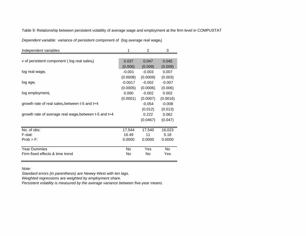
Table 9: Relationship between persistent volatility of average wage and employment at the firm level in COMPUSTAT

Dependent variable: variance of persistent component of (log average real wagef)

Independent variables 1 2 3 v of persistent component ( log real salesf) 0.037 0.047 0.045

(0.006) (0.009) (0.009)log real wagef -0.001 -0.003 0.007

(0.0008) (0.0009) (0.003)log agef -0.0017 -0.002 -0.007

(0.0005) (0.0006) (0.006)log employmentf 0.000 -0.002 0.002

(0.0001) (0.0007) (0.0016)growth rate of real salesf between t-5 and t+4 -0.054 -0.008

(0.012) (0.013)growth rate of average real wagef between t-5 and t+4 0.222 0.062

(0.0467) (0.047)

No. of obs: 17,544 17,540 16,023F-stat: 16.49 11 5.18Prob > F: 0.0000 0.0000 0.0000

Year Dummies No Yes NoFirm fixed effects & time trend No No Yes

Weighted regressions are weighted by employment share. Persistent volatility is measured by the average variance between five-year means.

Note: Standard errors (in parenthesis) are Newey-West with ten lags.

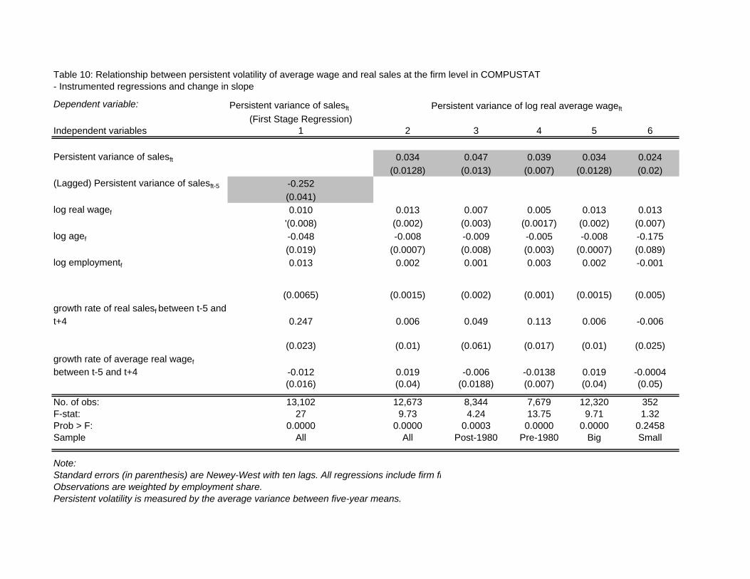
Table 10: Relationship between persistent volatility of average wage and real sales at the firm level in COMPUSTAT - Instrumented regressions and change in slope

Dependent variable: Persistent variance of salesft

(First Stage Regression)Independent variables 1 2 3 4 5 6 Persistent variance of salesft 0.034 0.047 0.039 0.034 0.024

(0.0128) (0.013) (0.007) (0.0128) (0.02)(Lagged) Persistent variance of salesft-5 -0.252

(0.041)log real wagef 0.010 0.013 0.007 0.005 0.013 0.013

'(0.008) (0.002) (0.003) (0.0017) (0.002) (0.007)log agef -0.048 -0.008 -0.009 -0.005 -0.008 -0.175

(0.019) (0.0007) (0.008) (0.003) (0.0007) (0.089)log employmentf 0.013 0.002 0.001 0.003 0.002 -0.001

(0.0065) (0.0015) (0.002) (0.001) (0.0015) (0.005)growth rate of real salesf between t-5 and t+4 0.247 0.006 0.049 0.113 0.006 -0.006

(0.023) (0.01) (0.061) (0.017) (0.01) (0.025)growth rate of average real wagef

between t-5 and t+4 -0.012 0.019 -0.006 -0.0138 0.019 -0.0004(0.016) (0.04) (0.0188) (0.007) (0.04) (0.05)

No. of obs: 13,102 12,673 8,344 7,679 12,320 352F-stat: 27 9.73 4.24 13.75 9.71 1.32Prob > F: 0.0000 0.0000 0.0003 0.0000 0.0000 0.2458Sample All All Post-1980 Pre-1980 Big Small

Observations are weighted by employment share. Persistent volatility is measured by the average variance between five-year means.

Note: Standard errors (in parenthesis) are Newey-West with ten lags. All regressions include firm fi

Persistent variance of log real average wageft

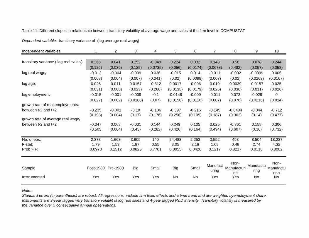
Table 11: Different slopes in relationship between transitory volatility of average wage and sales at the firm level in COMPUSTAT

Dependent variable: transitory variance of (log average real wagef)

Independent variables 1 2 3 4 5 6 7 8 9 10 transitory variance ( log real salesf) 0.265 0.041 0.252 -0.049 0.224 0.032 0.143 0.58 0.078 0.244

(0.126) (0.039) (0.125) (0.0735) (0.056) (0.0174) (0.0678) (0.482) (0.057) (0.058)log real wagef -0.012 -0.004 -0.009 0.036 -0.015 0.014 -0.011 -0.002 -0.0399 0.005

(0.008) (0.004) (0.007) (0.041) (0.02) (0.0098) (0.007) (0.02) (0.0269) (0.0167)log agef 0.025 0.011 0.0167 -0.312 0.0017 -0.006 0.019 0.0039 -0.0157 0.025

(0.031) (0.008) (0.023) (0.266) (0.0135) (0.0179) (0.026) (0.036) (0.011) (0.026)log employmentf -0.015 -0.001 -0.009 -0.1 -0.0148 -0.009 -0.011 0.073 -0.029 0

(0.027) (0.002) (0.0188) (0.07) (0.0158) (0.0116) (0.007) (0.076) (0.0216) (0.014)growth rate of real employmentsf

between t-2 and t+2 -0.235 -0.001 -0.18 -0.106 -0.397 -0.216 -0.145 -0.0404 -0.044 -0.712(0.198) (0.004) (0.17) (0.176) (0.258) (0.105) (0.187) (0.302) (0.14) (0.477)

growth rate of average real wagef

between t-2 and t+2 -0.047 0.063 -0.031 0.144 0.249 0.105 0.025 -0.361 0.158 0.306(0.505 (0.064) (0.43) (0.282) (0.426) (0.164) (0.494) (0.607) (0.36) (0.732)

No. of obs: 2,373 1,668 3,905 140 24,488 2,253 3,552 493 8,504 18,237F-stat: 1.79 1.53 1.87 0.55 3.05 2.18 1.68 0.48 2.74 4.32Prob > F: 0.0978 0.1512 0.0825 0.7701 0.0055 0.0426 0.1217 0.8217 0.0116 0.0002

Sample Post-1980 Pre-1980 Big Small Big Small Manufacturing

Non-Manufacturi

ng

Manufacturing

Non-Manufactu

ringInstrumented Yes Yes Yes Yes No No Yes Yes No No

Standard errors (in parenthesis) are robust. All regressions include firm fixed effects and a time trend and are weighted byemployment share. Instruments are 3-year lagged very transitory volatilit of log real sales and 4-year lagged R&D intensity. Transitory volatility is measured by the variance over 5 consecuative annual observations.

Note:

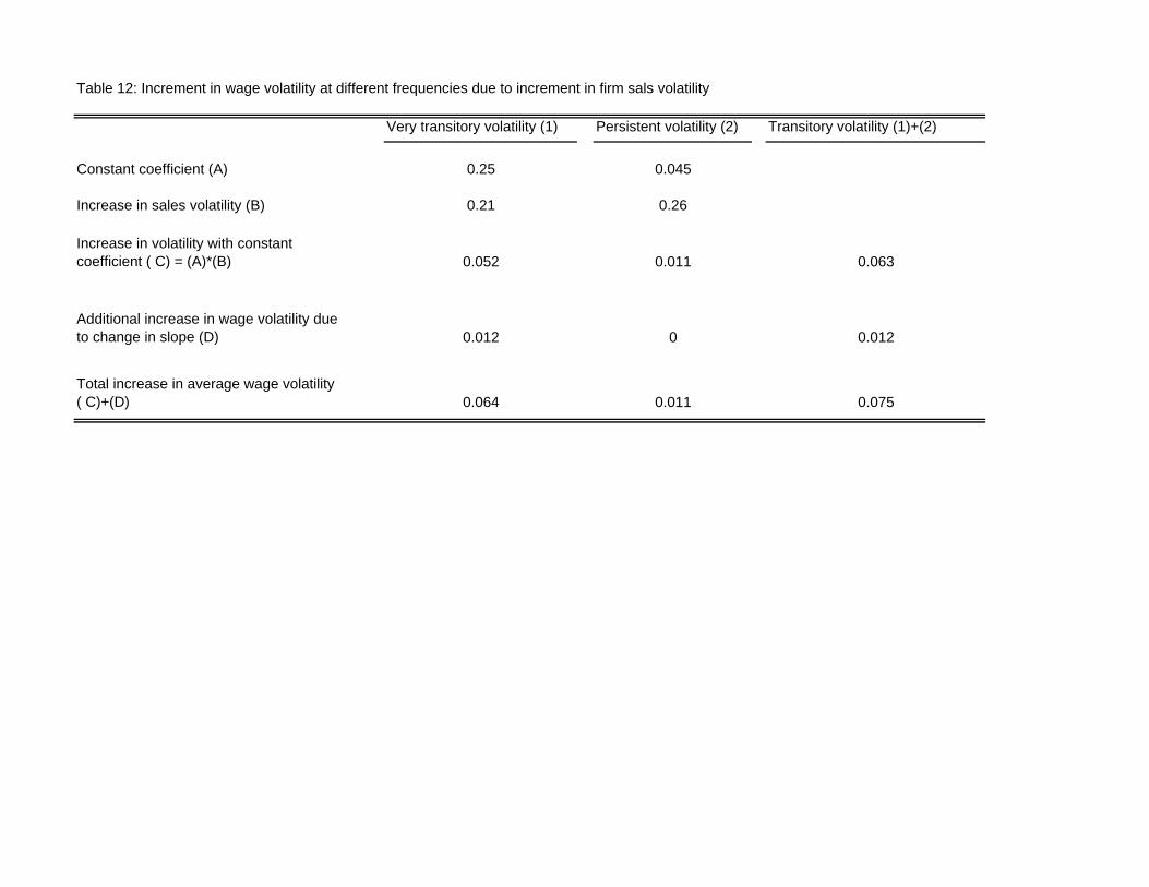
Table 12: Increment in wage volatility at different frequencies due to increment in firm sals volatility

Very transitory volatility (1) Persistent volatility (2) Transitory volatility (1)+(2)

Constant coefficient (A) 0.25 0.045

Increase in sales volatility (B) 0.21 0.26

Increase in volatility with constant coefficient ( C) = (A)*(B) 0.052 0.011 0.063

Additional increase in wage volatility due to change in slope (D) 0.012 0 0.012

Total increase in average wage volatility ( C)+(D) 0.064 0.011 0.075

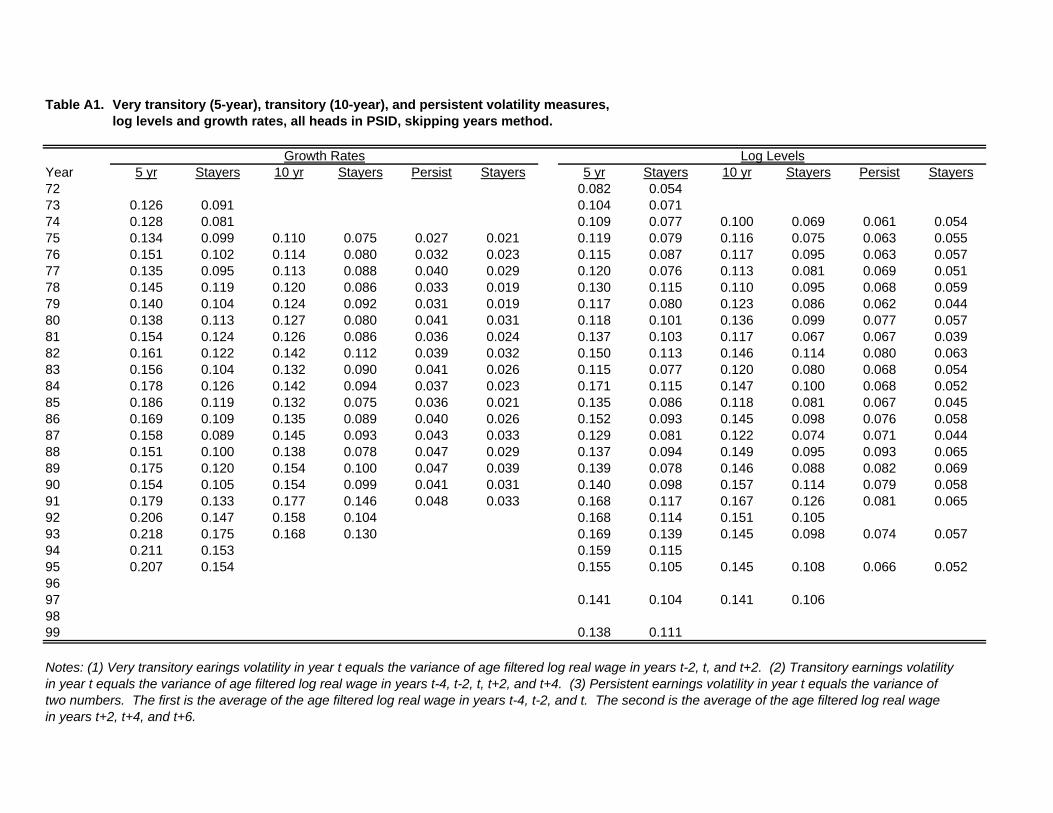
Table A1. Very transitory (5-year), transitory (10-year), and persistent volatility measures, log levels and growth rates, all heads in PSID, skipping years method.

Year 5 yr Stayers 10 yr Stayers Persist Stayers 5 yr Stayers 10 yr Stayers Persist Stayers72 0.082 0.05473 0.126 0.091 0.104 0.07174 0.128 0.081 0.109 0.077 0.100 0.069 0.061 0.05475 0.134 0.099 0.110 0.075 0.027 0.021 0.119 0.079 0.116 0.075 0.063 0.05576 0.151 0.102 0.114 0.080 0.032 0.023 0.115 0.087 0.117 0.095 0.063 0.05777 0.135 0.095 0.113 0.088 0.040 0.029 0.120 0.076 0.113 0.081 0.069 0.05178 0.145 0.119 0.120 0.086 0.033 0.019 0.130 0.115 0.110 0.095 0.068 0.05979 0.140 0.104 0.124 0.092 0.031 0.019 0.117 0.080 0.123 0.086 0.062 0.04480 0.138 0.113 0.127 0.080 0.041 0.031 0.118 0.101 0.136 0.099 0.077 0.05781 0.154 0.124 0.126 0.086 0.036 0.024 0.137 0.103 0.117 0.067 0.067 0.03982 0.161 0.122 0.142 0.112 0.039 0.032 0.150 0.113 0.146 0.114 0.080 0.06383 0.156 0.104 0.132 0.090 0.041 0.026 0.115 0.077 0.120 0.080 0.068 0.05484 0.178 0.126 0.142 0.094 0.037 0.023 0.171 0.115 0.147 0.100 0.068 0.05285 0.186 0.119 0.132 0.075 0.036 0.021 0.135 0.086 0.118 0.081 0.067 0.04586 0.169 0.109 0.135 0.089 0.040 0.026 0.152 0.093 0.145 0.098 0.076 0.05887 0.158 0.089 0.145 0.093 0.043 0.033 0.129 0.081 0.122 0.074 0.071 0.04488 0.151 0.100 0.138 0.078 0.047 0.029 0.137 0.094 0.149 0.095 0.093 0.06589 0.175 0.120 0.154 0.100 0.047 0.039 0.139 0.078 0.146 0.088 0.082 0.06990 0.154 0.105 0.154 0.099 0.041 0.031 0.140 0.098 0.157 0.114 0.079 0.05891 0.179 0.133 0.177 0.146 0.048 0.033 0.168 0.117 0.167 0.126 0.081 0.06592 0.206 0.147 0.158 0.104 0.168 0.114 0.151 0.10593 0.218 0.175 0.168 0.130 0.169 0.139 0.145 0.098 0.074 0.05794 0.211 0.153 0.159 0.11595 0.207 0.154 0.155 0.105 0.145 0.108 0.066 0.0529697 0.141 0.104 0.141 0.1069899 0.138 0.111

Notes: (1) Very transitory earings volatility in year t equals the variance of age filtered log real wage in years t-2, t, and t+2. (2) Transitory earnings volatilityin year t equals the variance of age filtered log real wage in years t-4, t-2, t, t+2, and t+4. (3) Persistent earnings volatility in year t equals the variance oftwo numbers. The first is the average of the age filtered log real wage in years t-4, t-2, and t. The second is the average of the age filtered log real wagein years t+2, t+4, and t+6.

Growth Rates Log Levels

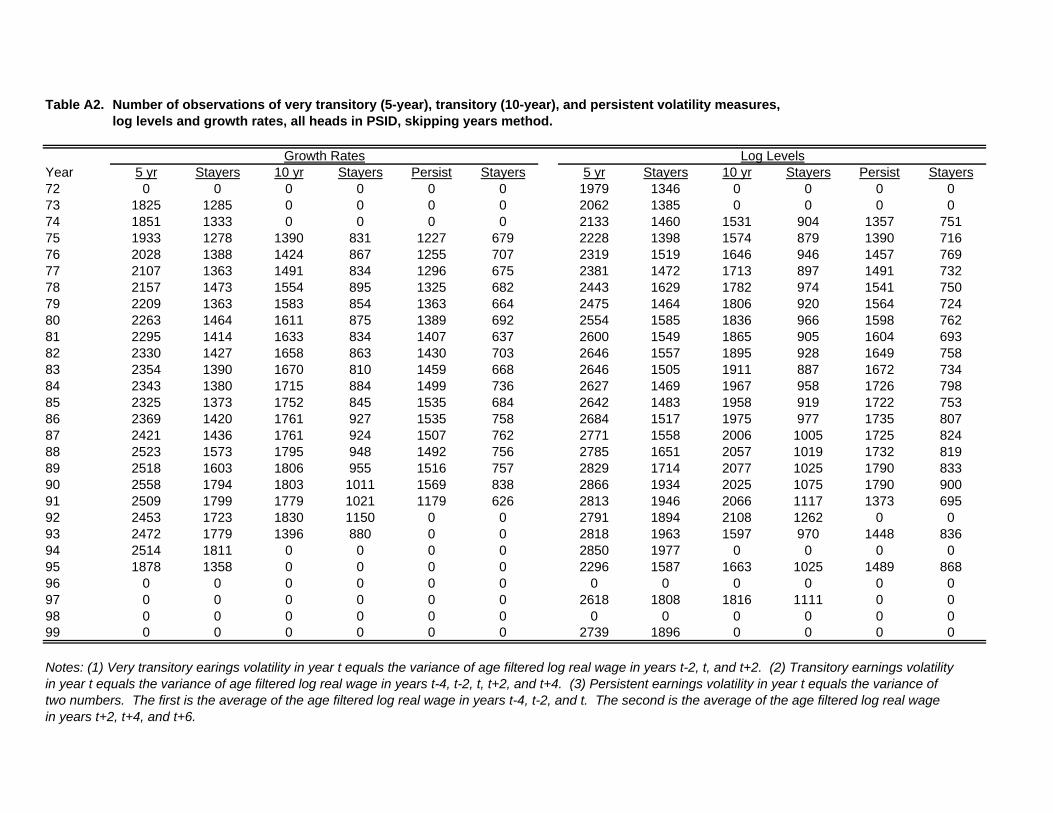
Table A2. Number of observations of very transitory (5-year), transitory (10-year), and persistent volatility measures, log levels and growth rates, all heads in PSID, skipping years method.

Year 5 yr Stayers 10 yr Stayers Persist Stayers 5 yr Stayers 10 yr Stayers Persist Stayers72 0 0 0 0 0 0 1979 1346 0 0 0 073 1825 1285 0 0 0 0 2062 1385 0 0 0 074 1851 1333 0 0 0 0 2133 1460 1531 904 1357 75175 1933 1278 1390 831 1227 679 2228 1398 1574 879 1390 71676 2028 1388 1424 867 1255 707 2319 1519 1646 946 1457 76977 2107 1363 1491 834 1296 675 2381 1472 1713 897 1491 73278 2157 1473 1554 895 1325 682 2443 1629 1782 974 1541 75079 2209 1363 1583 854 1363 664 2475 1464 1806 920 1564 72480 2263 1464 1611 875 1389 692 2554 1585 1836 966 1598 76281 2295 1414 1633 834 1407 637 2600 1549 1865 905 1604 69382 2330 1427 1658 863 1430 703 2646 1557 1895 928 1649 75883 2354 1390 1670 810 1459 668 2646 1505 1911 887 1672 73484 2343 1380 1715 884 1499 736 2627 1469 1967 958 1726 79885 2325 1373 1752 845 1535 684 2642 1483 1958 919 1722 75386 2369 1420 1761 927 1535 758 2684 1517 1975 977 1735 80787 2421 1436 1761 924 1507 762 2771 1558 2006 1005 1725 82488 2523 1573 1795 948 1492 756 2785 1651 2057 1019 1732 81989 2518 1603 1806 955 1516 757 2829 1714 2077 1025 1790 83390 2558 1794 1803 1011 1569 838 2866 1934 2025 1075 1790 90091 2509 1799 1779 1021 1179 626 2813 1946 2066 1117 1373 69592 2453 1723 1830 1150 0 0 2791 1894 2108 1262 0 093 2472 1779 1396 880 0 0 2818 1963 1597 970 1448 83694 2514 1811 0 0 0 0 2850 1977 0 0 0 095 1878 1358 0 0 0 0 2296 1587 1663 1025 1489 86896 0 0 0 0 0 0 0 0 0 0 0 097 0 0 0 0 0 0 2618 1808 1816 1111 0 098 0 0 0 0 0 0 0 0 0 0 0 099 0 0 0 0 0 0 2739 1896 0 0 0 0



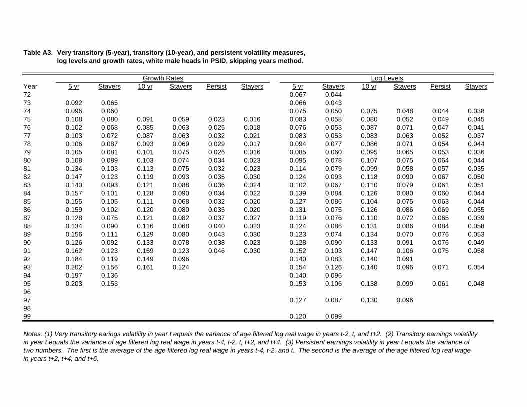
Table A3. Very transitory (5-year), transitory (10-year), and persistent volatility measures, log levels and growth rates, white male heads in PSID, skipping years method.

Year 5 yr Stayers 10 yr Stayers Persist Stayers 5 yr Stayers 10 yr Stayers Persist Stayers72 0.067 0.04473 0.092 0.065 0.066 0.04374 0.096 0.060 0.075 0.050 0.075 0.048 0.044 0.03875 0.108 0.080 0.091 0.059 0.023 0.016 0.083 0.058 0.080 0.052 0.049 0.04576 0.102 0.068 0.085 0.063 0.025 0.018 0.076 0.053 0.087 0.071 0.047 0.04177 0.103 0.072 0.087 0.063 0.032 0.021 0.083 0.053 0.083 0.063 0.052 0.03778 0.106 0.087 0.093 0.069 0.029 0.017 0.094 0.077 0.086 0.071 0.054 0.04479 0.105 0.081 0.101 0.075 0.026 0.016 0.085 0.060 0.095 0.065 0.053 0.03680 0.108 0.089 0.103 0.074 0.034 0.023 0.095 0.078 0.107 0.075 0.064 0.04481 0.134 0.103 0.113 0.075 0.032 0.023 0.114 0.079 0.099 0.058 0.057 0.03582 0.147 0.123 0.119 0.093 0.035 0.030 0.124 0.093 0.118 0.090 0.067 0.05083 0.140 0.093 0.121 0.088 0.036 0.024 0.102 0.067 0.110 0.079 0.061 0.05184 0.157 0.101 0.128 0.090 0.034 0.022 0.139 0.084 0.126 0.080 0.060 0.04485 0.155 0.105 0.111 0.068 0.032 0.020 0.127 0.086 0.104 0.075 0.063 0.04486 0.159 0.102 0.120 0.080 0.035 0.020 0.131 0.075 0.126 0.086 0.069 0.05587 0.128 0.075 0.121 0.082 0.037 0.027 0.119 0.076 0.110 0.072 0.065 0.03988 0.134 0.090 0.116 0.068 0.040 0.023 0.124 0.086 0.131 0.086 0.084 0.05889 0.156 0.111 0.129 0.080 0.043 0.030 0.123 0.074 0.134 0.070 0.076 0.05390 0.126 0.092 0.133 0.078 0.038 0.023 0.128 0.090 0.133 0.091 0.076 0.04991 0.162 0.123 0.159 0.123 0.046 0.030 0.152 0.103 0.147 0.106 0.075 0.05892 0.184 0.119 0.149 0.096 0.140 0.083 0.140 0.09193 0.202 0.156 0.161 0.124 0.154 0.126 0.140 0.096 0.071 0.05494 0.197 0.136 0.140 0.09695 0.203 0.153 0.153 0.106 0.138 0.099 0.061 0.0489697 0.127 0.087 0.130 0.0969899 0.120 0.099



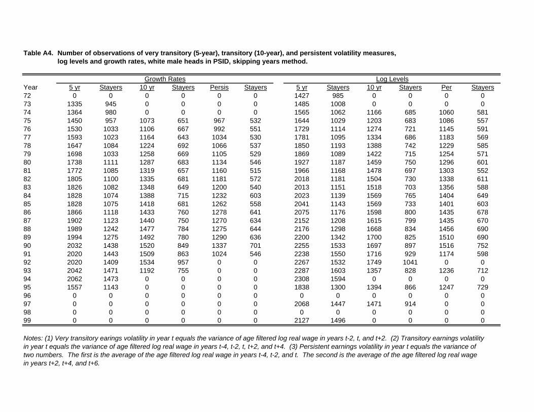
Table A4. Number of observations of very transitory (5-year), transitory (10-year), and persistent volatility measures, log levels and growth rates, white male heads in PSID, skipping years method.

Year 5 yr Stayers 10 yr Stayers Persis Stayers 5 yr Stayers 10 yr Stayers Per Stayers72 0 0 0 0 0 0 1427 985 0 0 0 073 1335 945 0 0 0 0 1485 1008 0 0 0 074 1364 980 0 0 0 0 1565 1062 1166 685 1060 58175 1450 957 1073 651 967 532 1644 1029 1203 683 1086 55776 1530 1033 1106 667 992 551 1729 1114 1274 721 1145 59177 1593 1023 1164 643 1034 530 1781 1095 1334 686 1183 56978 1647 1084 1224 692 1066 537 1850 1193 1388 742 1229 58579 1698 1033 1258 669 1105 529 1869 1089 1422 715 1254 57180 1738 1111 1287 683 1134 546 1927 1187 1459 750 1296 60181 1772 1085 1319 657 1160 515 1966 1168 1478 697 1303 55282 1805 1100 1335 681 1181 572 2018 1181 1504 730 1338 61183 1826 1082 1348 649 1200 540 2013 1151 1518 703 1356 58884 1828 1074 1388 715 1232 603 2023 1139 1569 765 1404 64985 1828 1075 1418 681 1262 558 2041 1143 1569 733 1401 60386 1866 1118 1433 760 1278 641 2075 1176 1598 800 1435 67887 1902 1123 1440 750 1270 634 2152 1208 1615 799 1435 67088 1989 1242 1477 784 1275 644 2176 1298 1668 834 1456 69089 1994 1275 1492 780 1290 636 2200 1342 1700 825 1510 69090 2032 1438 1520 849 1337 701 2255 1533 1697 897 1516 75291 2020 1443 1509 863 1024 546 2238 1550 1716 929 1174 59892 2020 1409 1534 957 0 0 2267 1532 1749 1041 0 093 2042 1471 1192 755 0 0 2287 1603 1357 828 1236 71294 2062 1473 0 0 0 0 2308 1594 0 0 0 095 1557 1143 0 0 0 0 1838 1300 1394 866 1247 72996 0 0 0 0 0 0 0 0 0 0 0 097 0 0 0 0 0 0 2068 1447 1471 914 0 098 0 0 0 0 0 0 0 0 0 0 0 099 0 0 0 0 0 0 2127 1496 0 0 0 0



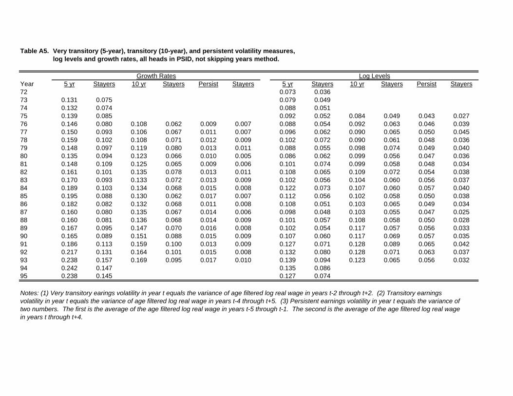
Table A5. Very transitory (5-year), transitory (10-year), and persistent volatility measures, log levels and growth rates, all heads in PSID, not skipping years method.

Year 5 yr Stayers 10 yr Stayers Persist Stayers 5 yr Stayers 10 yr Stayers Persist Stayers72 0.073 0.03673 0.131 0.075 0.079 0.04974 0.132 0.074 0.088 0.05175 0.139 0.085 0.092 0.052 0.084 0.049 0.043 0.02776 0.146 0.080 0.108 0.062 0.009 0.007 0.088 0.054 0.092 0.063 0.046 0.03977 0.150 0.093 0.106 0.067 0.011 0.007 0.096 0.062 0.090 0.065 0.050 0.04578 0.159 0.102 0.108 0.071 0.012 0.009 0.102 0.072 0.090 0.061 0.048 0.03679 0.148 0.097 0.119 0.080 0.013 0.011 0.088 0.055 0.098 0.074 0.049 0.04080 0.135 0.094 0.123 0.066 0.010 0.005 0.086 0.062 0.099 0.056 0.047 0.03681 0.148 0.109 0.125 0.065 0.009 0.006 0.101 0.074 0.099 0.058 0.048 0.03482 0.161 0.101 0.135 0.078 0.013 0.011 0.108 0.065 0.109 0.072 0.054 0.03883 0.170 0.093 0.133 0.072 0.013 0.009 0.102 0.056 0.104 0.060 0.056 0.03784 0.189 0.103 0.134 0.068 0.015 0.008 0.122 0.073 0.107 0.060 0.057 0.04085 0.195 0.088 0.130 0.062 0.017 0.007 0.112 0.056 0.102 0.058 0.050 0.03886 0.182 0.082 0.132 0.068 0.011 0.008 0.108 0.051 0.103 0.065 0.049 0.03487 0.160 0.080 0.135 0.067 0.014 0.006 0.098 0.048 0.103 0.055 0.047 0.02588 0.160 0.081 0.136 0.068 0.014 0.009 0.101 0.057 0.108 0.058 0.050 0.02889 0.167 0.095 0.147 0.070 0.016 0.008 0.102 0.054 0.117 0.057 0.056 0.03390 0.165 0.089 0.151 0.088 0.015 0.009 0.107 0.060 0.117 0.069 0.057 0.03591 0.186 0.113 0.159 0.100 0.013 0.009 0.127 0.071 0.128 0.089 0.065 0.04292 0.217 0.131 0.164 0.101 0.015 0.008 0.132 0.080 0.128 0.071 0.063 0.03793 0.238 0.157 0.169 0.095 0.017 0.010 0.139 0.094 0.123 0.065 0.056 0.03294 0.242 0.147 0.135 0.08695 0.238 0.145 0.127 0.074

Notes: (1) Very transitory earings volatility in year t equals the variance of age filtered log real wage in years t-2 through t+2. (2) Transitory earnings volatility in year t equals the variance of age filtered log real wage in years t-4 through t+5. (3) Persistent earnings volatility in year t equals the variance oftwo numbers. The first is the average of the age filtered log real wage in years t-5 through t-1. The second is the average of the age filtered log real wagein years t through t+4.


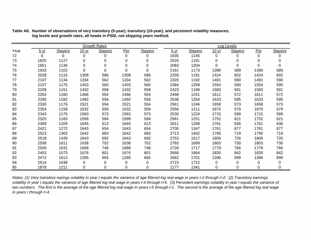
Table A6. Number of observations of very transitory (5-year), transitory (10-year), and persistent volatility measures, log levels and growth rates, all heads in PSID, not skipping years method.

Year 5 yr Stayers 10 yr Stayers Per Stayers 5 yr Stayers 10 yr Stayers Per Stayers72 0 0 0 0 0 0 1935 1145 0 0 0 073 1825 1127 0 0 0 0 2020 1191 0 0 0 074 1851 1136 0 0 0 0 2083 1204 0 0 0 075 1933 1102 0 0 0 0 2161 1173 1390 589 1390 58976 2028 1115 1308 586 1308 586 2259 1191 1424 602 1424 60277 2107 1134 1334 562 1334 562 2320 1192 1491 590 1491 59078 2157 1175 1403 560 1403 560 2384 1258 1554 590 1554 59079 2209 1151 1432 558 1432 558 2423 1199 1583 591 1583 59180 2263 1180 1466 554 1466 554 2498 1241 1611 572 1611 57281 2295 1182 1492 556 1492 556 2538 1254 1633 595 1633 59582 2330 1176 1521 554 1521 554 2561 1246 1658 573 1658 57383 2354 1158 1532 559 1532 559 2556 1211 1670 579 1670 57984 2343 1175 1563 573 1563 573 2530 1224 1715 599 1715 59985 2325 1183 1599 594 1599 594 2561 1251 1752 621 1752 62186 2369 1209 1645 613 1645 613 2611 1268 1761 636 1761 63687 2421 1272 1643 654 1643 654 2700 1347 1761 677 1761 67788 2523 1363 1642 683 1642 683 2713 1402 1795 719 1795 71989 2518 1439 1643 692 1643 692 2753 1517 1806 726 1806 72690 2558 1611 1638 702 1638 702 2783 1699 1803 730 1803 73091 2509 1631 1668 748 1668 748 2728 1717 1779 766 1779 76692 2453 1573 1676 801 1676 801 2668 1664 1830 842 1830 84293 2472 1613 1285 665 1285 665 2682 1701 1396 699 1396 69994 2514 1638 0 0 0 0 2723 1722 0 0 0 095 1878 1211 0 0 0 0 2177 1341 0 0 0 0



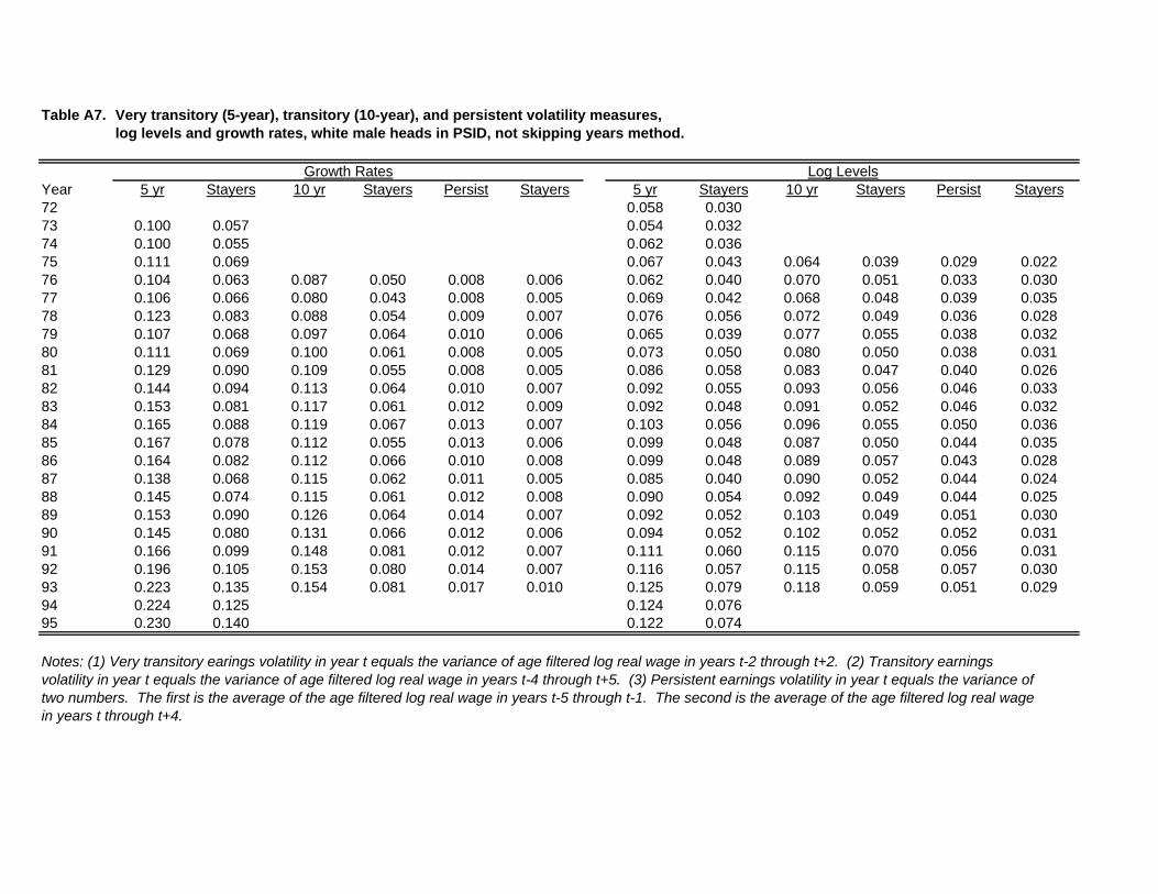
Table A7. Very transitory (5-year), transitory (10-year), and persistent volatility measures, log levels and growth rates, white male heads in PSID, not skipping years method.

Year 5 yr Stayers 10 yr Stayers Persist Stayers 5 yr Stayers 10 yr Stayers Persist Stayers72 0.058 0.03073 0.100 0.057 0.054 0.03274 0.100 0.055 0.062 0.03675 0.111 0.069 0.067 0.043 0.064 0.039 0.029 0.02276 0.104 0.063 0.087 0.050 0.008 0.006 0.062 0.040 0.070 0.051 0.033 0.03077 0.106 0.066 0.080 0.043 0.008 0.005 0.069 0.042 0.068 0.048 0.039 0.03578 0.123 0.083 0.088 0.054 0.009 0.007 0.076 0.056 0.072 0.049 0.036 0.02879 0.107 0.068 0.097 0.064 0.010 0.006 0.065 0.039 0.077 0.055 0.038 0.03280 0.111 0.069 0.100 0.061 0.008 0.005 0.073 0.050 0.080 0.050 0.038 0.03181 0.129 0.090 0.109 0.055 0.008 0.005 0.086 0.058 0.083 0.047 0.040 0.02682 0.144 0.094 0.113 0.064 0.010 0.007 0.092 0.055 0.093 0.056 0.046 0.03383 0.153 0.081 0.117 0.061 0.012 0.009 0.092 0.048 0.091 0.052 0.046 0.03284 0.165 0.088 0.119 0.067 0.013 0.007 0.103 0.056 0.096 0.055 0.050 0.03685 0.167 0.078 0.112 0.055 0.013 0.006 0.099 0.048 0.087 0.050 0.044 0.03586 0.164 0.082 0.112 0.066 0.010 0.008 0.099 0.048 0.089 0.057 0.043 0.02887 0.138 0.068 0.115 0.062 0.011 0.005 0.085 0.040 0.090 0.052 0.044 0.02488 0.145 0.074 0.115 0.061 0.012 0.008 0.090 0.054 0.092 0.049 0.044 0.02589 0.153 0.090 0.126 0.064 0.014 0.007 0.092 0.052 0.103 0.049 0.051 0.03090 0.145 0.080 0.131 0.066 0.012 0.006 0.094 0.052 0.102 0.052 0.052 0.03191 0.166 0.099 0.148 0.081 0.012 0.007 0.111 0.060 0.115 0.070 0.056 0.03192 0.196 0.105 0.153 0.080 0.014 0.007 0.116 0.057 0.115 0.058 0.057 0.03093 0.223 0.135 0.154 0.081 0.017 0.010 0.125 0.079 0.118 0.059 0.051 0.02994 0.224 0.125 0.124 0.07695 0.230 0.140 0.122 0.074



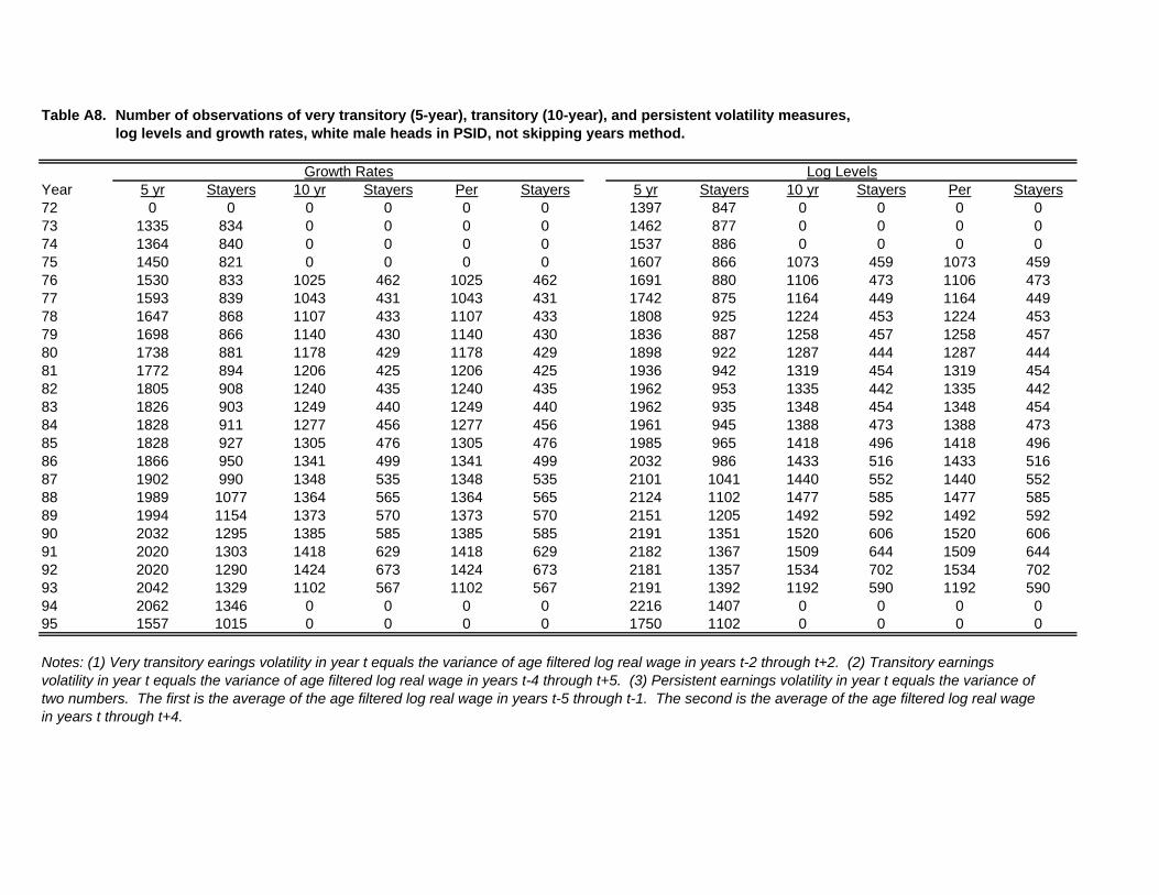
Table A8. Number of observations of very transitory (5-year), transitory (10-year), and persistent volatility measures, log levels and growth rates, white male heads in PSID, not skipping years method.

Year 5 yr Stayers 10 yr Stayers Per Stayers 5 yr Stayers 10 yr Stayers Per Stayers72 0 0 0 0 0 0 1397 847 0 0 0 073 1335 834 0 0 0 0 1462 877 0 0 0 074 1364 840 0 0 0 0 1537 886 0 0 0 075 1450 821 0 0 0 0 1607 866 1073 459 1073 45976 1530 833 1025 462 1025 462 1691 880 1106 473 1106 47377 1593 839 1043 431 1043 431 1742 875 1164 449 1164 44978 1647 868 1107 433 1107 433 1808 925 1224 453 1224 45379 1698 866 1140 430 1140 430 1836 887 1258 457 1258 45780 1738 881 1178 429 1178 429 1898 922 1287 444 1287 44481 1772 894 1206 425 1206 425 1936 942 1319 454 1319 45482 1805 908 1240 435 1240 435 1962 953 1335 442 1335 44283 1826 903 1249 440 1249 440 1962 935 1348 454 1348 45484 1828 911 1277 456 1277 456 1961 945 1388 473 1388 47385 1828 927 1305 476 1305 476 1985 965 1418 496 1418 49686 1866 950 1341 499 1341 499 2032 986 1433 516 1433 51687 1902 990 1348 535 1348 535 2101 1041 1440 552 1440 55288 1989 1077 1364 565 1364 565 2124 1102 1477 585 1477 58589 1994 1154 1373 570 1373 570 2151 1205 1492 592 1492 59290 2032 1295 1385 585 1385 585 2191 1351 1520 606 1520 60691 2020 1303 1418 629 1418 629 2182 1367 1509 644 1509 64492 2020 1290 1424 673 1424 673 2181 1357 1534 702 1534 70293 2042 1329 1102 567 1102 567 2191 1392 1192 590 1192 59094 2062 1346 0 0 0 0 2216 1407 0 0 0 095 1557 1015 0 0 0 0 1750 1102 0 0 0 0



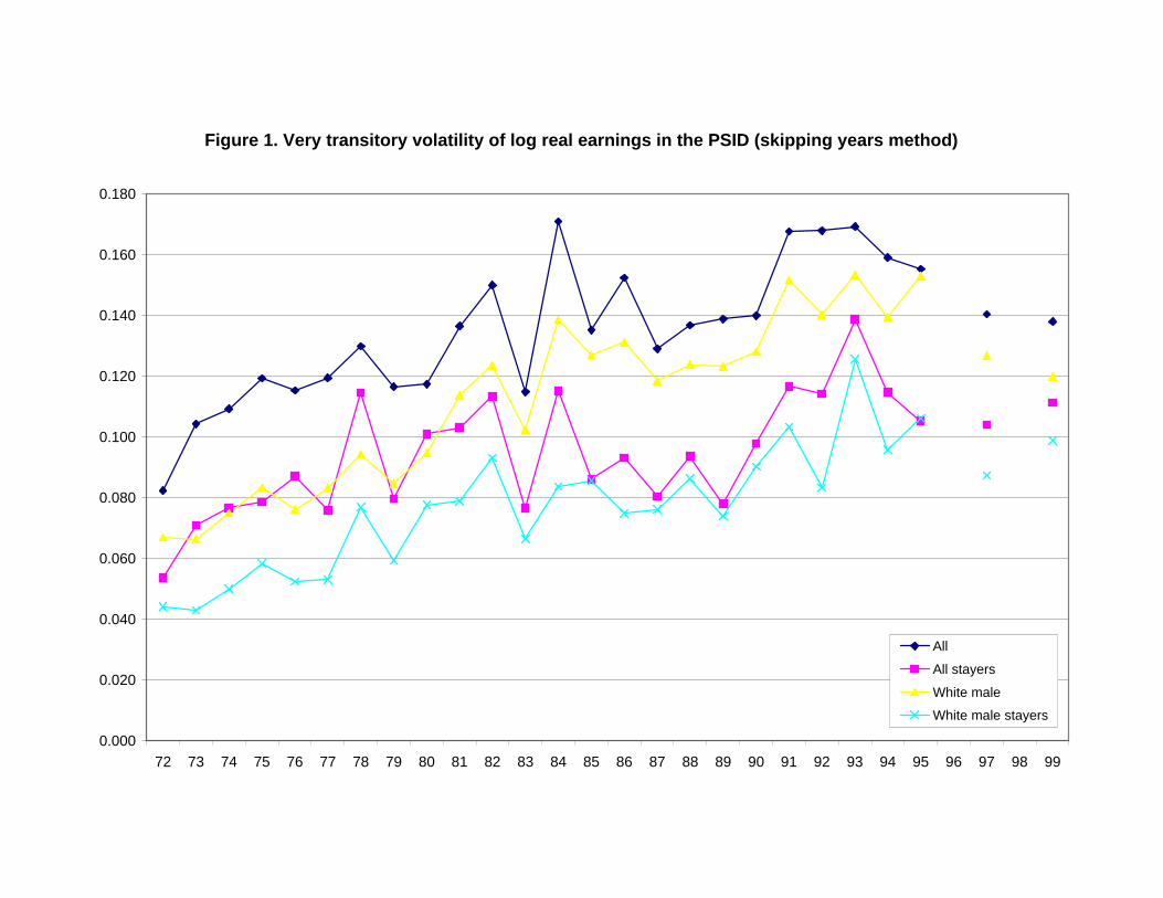
Figure 1. Very transitory volatility of log real earnings in the PSID (skipping years method)

0.000

0.020

0.040

0.060

0.080

0.100

0.120

0.140

0.160

0.180

72 73 74 75 76 77 78 79 80 81 82 83 84 85 86 87 88 89 90 91 92 93 94 95 96 97 98 99

All

All stayers

White male

White male stayers

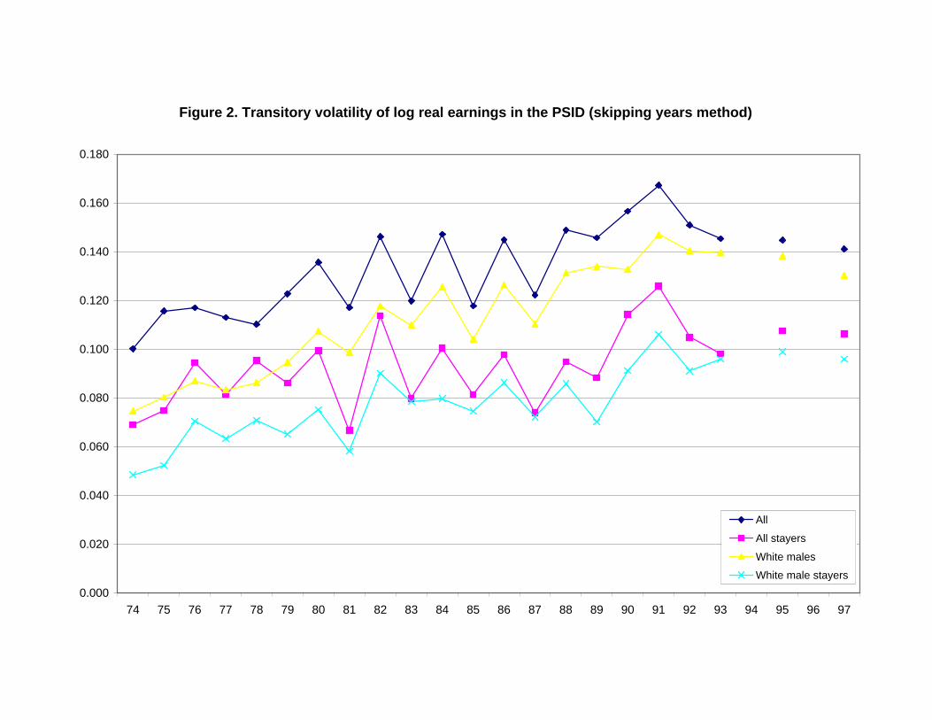
Figure 2. Transitory volatility of log real earnings in the PSID (skipping years method)

0.000

0.020

0.040

0.060

0.080

0.100

0.120

0.140

0.160

0.180

74 75 76 77 78 79 80 81 82 83 84 85 86 87 88 89 90 91 92 93 94 95 96 97

All

All stayers

White males

White male stayers

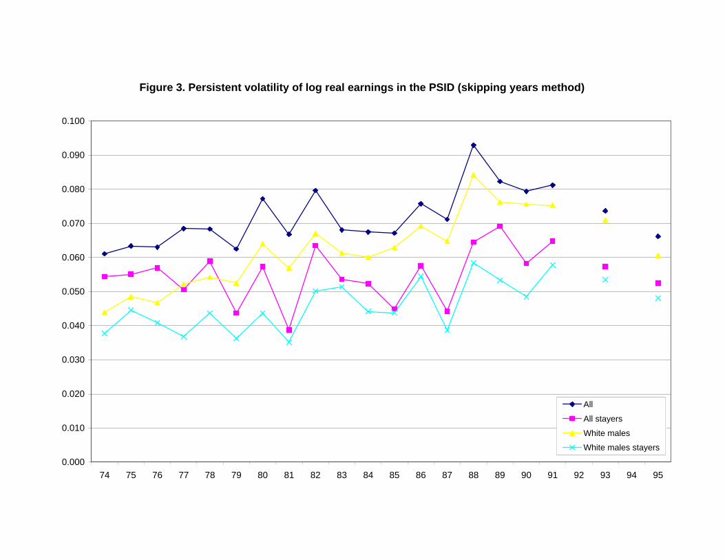
Figure 3. Persistent volatility of log real earnings in the PSID (skipping years method)

0.000

0.010

0.020

0.030

0.040

0.050

0.060

0.070

0.080

0.090

0.100

74 75 76 77 78 79 80 81 82 83 84 85 86 87 88 89 90 91 92 93 94 95

All

All stayers

White males

White males stayers

turbulent firms, turbulent wages? - harvard … files/09-057.pdf · turbulent firms, turbulent...

Documents