turbulent mixing by breaking gravity wavesfischer/gc/dornbrack.pdf · turbulent mixing by breaking...

J. Fluid Mech. (1998), vol. 375, pp. 113–141. Printed in the United Kingdom

c© 1998 Cambridge University Press

113

Turbulent mixing by breaking gravity waves

By A N D R E A S D O R N B R A C KDLR Oberpfaffenhofen, Institut fur Physik der Atmosphare, D-82230 Wessling, Germany

(Received 4 July 1996 and in revised form 10 July 1998)

The characteristics of turbulence caused by three-dimensional breaking of internalgravity waves beneath a critical level are investigated by means of high-resolutionnumerical simulations. The flow evolves in three stages. In the first one the flow istwo-dimensional: internal gravity waves propagate vertically upwards and create aconvectively unstable region beneath the critical level. Convective instability leads toturbulent breakdown in the second stage. The developing three-dimensional mixed re-gion is organized into shear-driven overturning rolls in the plane of wave propagationand into counter-rotating streamwise vortices in the spanwise plane. The productionof turbulent kinetic energy by shear is maximum. In the last stage, shear productionand mechanical dissipation of turbulent kinetic energy balance.

The evolution of the flow depends on topographic parameters (wavelength and am-plitude), on shear and stratification as well as on viscosity. Here, only the implicationsof the viscosity for the instability structure and evolution in terms of the Reynoldsnumber are considered. Smaller viscosity leads to earlier onset of convective insta-bility and overturning waves. However, viscosity retards the onset of smaller-scalethree-dimensional instabilities and leads to a reduced momentum transfer to the meanflow below the critical level. Hence, the formation of secondary overturning rolls issustained by lower viscosity.

The budgets of total kinetic and potential energies are calculated. Although thedomain-averaged turbulent kinetic energy is less than 1% of the total kinetic energy,it is strong enough to form a patchy and intermittent turbulent mixed layer belowthe critical level.

1. IntroductionBreaking gravity waves exert a significant drag on the atmospheric flow. Knowledge

of their locations and magnitude is essential for parameterizing drag in numericalmodels predicting weather or climate. Current theoretical and computational studiesof momentum and mass transfer in stably stratified flows focus mainly on provid-ing useful parameterizations of this effect (see for example Bacmeister et al. 1994;Kim & Arakawa 1995; Broad 1995; Shutts 1995). In addition, small-scale mixing bybreaking gravity waves in the free atmosphere influences the horizontal and verticaldistributions of constituents, e.g. exhaust gases from high flying aircraft (Schumannet al. 1995; Schilling & Etling 1996; Dornbrack & Durbeck 1998). Furthermore, mi-crophysical and chemical calculations require a knowledge of the small-scale thermaland dynamical structure of internal gravity waves that lead to moisture and temper-ature conditions which promote the nucleation and growth of aerosol particles (Peteret al. 1995; Carslaw et al. 1998a, b).

114 A. Dornbrack

In the present paper, the life-cycle of vertically propagating internal gravity wavestrapped by a critical level is simulated. The high-resolution numerical simulationsare restricted to idealized flow conditions where a linear shear flow over a sinusoidalsurface excites internal gravity waves in a stably stratified flow. The critical level(the height where the phase speed of a wave equals the mean flow speed) stronglymodifies vertical wave propagation: only very small-amplitude waves are transmittedbeyond the critical level. Booker & Bretherton (1967) used linear inviscid theory todemonstrate that as a gravity wave propagates through the critical level, its amplitudeis reduced by a factor exp[−2π(Ric − 0.25)1/2], where Ric > 0.25 is the Richardsonnumber at the critical level. Beneath the critical level wave energy is absorbed bymean flow. Depending on the wave energy, shear and stratification of the basicflow, turbulence can be generated which cascades kinetic energy to smaller scales. Asummary of recent theoretical approaches to the critical level problem can be foundin Baines (1995, chapter 4.11).

Worthington & Thomas (1996), who observed the absorption of mountain waves atcritical layers by radar on the west coast of Wales, could identify enhanced turbulencebeneath the critical layer from the broadening of the spectral width of the radar echo.The wave behaviour below a critical level was studied in the laboratory under well-defined conditions of shear, stability and wave excitation by Thorpe (1981), Koop &McGee (1986), and Delisi & Dunkerton (1989). These mostly qualitative observationsare restricted either to flows where the wave energy is small and the flow does notreach overturning or to conditions where three-dimensional structures begin to evolve.So far, measurements of three-dimensional mixed layers after overturning have notbeen undertaken.

Most numerical investigations of gravity wave–critical layer interaction considertwo-dimensional problems (e.g. Fritts 1982; Winters & d’Asaro 1989; Dunkerton &Robins 1992; Schilling & Etling 1996). More recently, Winters & d’Asaro (1994),Dornbrack, Gerz & Schumann (1995), Fritts, Garten & Andreassen (1996), andGrubisic & Smolarkiewicz (1997) tackled the problem by three-dimensional numericalsimulations. Although the wave–mean flow interaction is essentially two-dimensionalin its early stage of flow evolution, these latest investigations found fundamently dif-ferent dynamics of wave instability in three dimensions compared to two-dimensionalones. Winters & d’Asaro (1994) found three-dimensional instability developing by atransverse convective instability of the two-dimensional wave. Fritts et al. (1996) drewspecial attention to flows where the mean shear is at an angle to the direction of wavepropagation. For this case, the instability structures are aligned with the backgroundshear flow rather than in the direction of wave propagation. They found less rapidgrowth compared to the parallel shear flow case. Grubisic & Smolarkiewicz (1997)studied the effect of the critical level on the airflow past an isolated mountain andextended previous studies that were restricted to two-dimensional wave excitation.

Our previous studies have concentrated on two aspects of gravity wave–criticallayer interaction. In Dornbrack & Nappo (1997), results from a two-dimensionalversion of the numerical code used in the present study were successfully comparedwith the tank experiment of Thorpe (1981). Because of the limited time of observationdue to the finite length of the tilted tube, only results at the early and quasi-linearstage of flow evolution could be considered. Therefore, the present study can beunderstood as an extension of Thorpe’s tank experiment by means of high-resolutionnumerical modelling for times far beyond the point of first instability. In Dornbracket al. (1995), the three-dimensional flow evolution using two different formulationsof viscosity was investigated: constant viscosity in a direct numerical simulation

Turbulent mixing by breaking gravity waves 115

(DNS) and flow-dependent viscosity as a function of the local shear perturbation andstability in a large-eddy simulation (LES). Both simulations behave similarly in theearly, almost two-dimensional stage of gravity wave–critical level interaction. Whenthe flow becomes nonlinear its structure consists of persistent small-scale overturningwaves in the DNS whereas the primary, convectively unstable region collapses rapidlyinto three-dimensional turbulence in the LES. These results show that convectivelyoverturning regions always form in the same way but the details of subsequentbreaking and the resulting structure of the mixed layer depend on the effectiveReynolds number of the flow. With sufficient viscous damping, three-dimensionalturbulent convective instabilities are more easily suppressed than two-dimensionallaminar overturning. From this study it was concluded that the use of a combinationof constant and flow-dependent subgrid-scale viscosity is necessary for a correctsimulation of the transition from two-dimensional wavy motion to three-dimensionalturbulence.

This paper considers flow regimes where the excitation is strong enough to overturngravity waves and where the net result to be expected is a horizontally homogeneousmixed layer. The main objective of this study is a detailed description of the dynamicsand energetics of this three-dimensional breaking. The following questions are to beanswered: What are the details of breaking? What is the role of viscosity? What arethe characteristics of turbulence generated by breaking gravity waves? How muchmean flow energy is transferred to waves, how much to turbulence? Finally, the studyshould provide fundamental knowledge for the physical understanding of the gravitywave–critical layer interaction and for its parameterization in large-scale models.

The paper is organized as follows. Section 2 briefly reviews the numerical method,describes its initial and boundary conditions, and introduces essential parameters. Adetailed description of the gravity wave breaking is given in § 3. Section 4 studies theimplications of viscosity on the instability structure and discusses the spectra for flowsof different Reynolds numbers. Section 5 investigates the energetics and estimates themixing efficiency of the breaking process. Similarities and differences between ourresults and previous, three-dimensional studies are discussed in § 6.

2. Simulation methodThe computational method is described in Dornbrack et al. (1995) and here only its

essential properties are repeated. The numerical scheme integrates the non-hydrostaticBoussinesq equations in three dimensions and as a function of time:

∂

∂xd(ρ0VG

dquq)

= 0 , (2.1)

∂

∂t(Vui) +

∂

∂xd(VGdququi

)= − 1

ρ0

∂

∂xg(VGgip

)− ∂

∂xd(Gds (VFis)

)+ V g

θ

ϑ0

δ3i, i = 1, 2, 3. (2.2)

Additionally, an equation for the temperature fluctuations

∂

∂t(Vθ) +

∂

∂xd(VGdquqθ

)+ Vu3

dΘ

dx3

= − ∂

∂xd(Gdr (VQr)

)(2.3)

is solved. The governing equations (2.1) to (2.3) are formulated for the Cartesiancoordinates (x, y, z) as a function of curvilinear coordinates (x, y, z) according to the

116 A. Dornbrack

H

zcrit H

0 DU2 U(z)– DU

20

Critical layer

λ

δLy

H

zcrit

1 1+ DH2 H(z)1– DH

2

Figure 1. Schematic sketch of the computational domain and the model set-up. The critical layerzcrit is defined by U = 0. The wave amplitude is δ = 0.03125H and the wavelength is λ = 1.5625H .The velocity and temperature differences across the vertical depth H are chosen in such a mannerthat the bulk Richardson number RiB is approximately 1.1 at the beginning.

transformation x = x, y = y, z = η(x, z). The Jacobian of the transformation isV = Det[Gij]−1 with Gij = ∂xi/∂xj . Here, η(x, z) = H (z − h)/(H − h) maps thedomain above the wavy surface with height h(x) = δ cos kxx, where kx = 2π/λ, andbelow a plane top surface at z = H into a rectangular transformed domain. Thewave amplitude is δ = 0.03125H and the wavelength is λ = 1.5625H . These valuesare taken from a comparison of our numerical results with the tank experiment ofThorpe (1981), see Dornbrack et al. (1995). Figure 1 shows the computational domainof height H , length λ and width λ/5.

The governing equations are approximated by finite differences on a staggered gridwith (nx, ny, nz) = (150, 30, 96) mesh cells. In the horizontal directions the grid spacingis equidistant (∆x = ∆y = H/nz). A higher resolution close to the critical level isachieved by transforming the vertical coordinate η on a non-equidistant grid using

η∗k =H

2

{α sinh

[arcsinh(α−1)

(2k − 1

nz− 1

)]+ 1

}, k = 1, 2, . . . , nz + 1. (2.4)

The parameter α = 0.1 is chosen so that the grid spacing is reduced by one order ofmagnitude from its surface value to the value at the critical level.

The diffusive fluxes in (2.2) and (2.3) are calculated by means of a first-order closure

VFij = −KM V2Dij , VQi = −KH

∂

∂xr(VGriθ

), (2.5)

where the deformation tensor Dij in terrain-following coordinates reads

Dij =1

2

1

V

∂

∂xr(VGrjui + VGriuj

). (2.6)

The subgrid-scale diffusivities KM and KH are modelled as the sum of a uniform anda flow-dependent eddy viscosity according to

KM =1

Re+ νturb and KH =

1

RePr+

νturb

P rturb, (2.7)

with Re = ∆UH/νM and Pr = νM/γ. The velocity difference across the vertical depthH is ∆U, νM denotes the kinematic viscosity, γ is the thermal conductivity, and Prturb =1. For this subgrid-scale model different Reynolds numbers Re = 2 × 104, 3 × 104,and 5 × 104 are tested. For the simulation presented in § 3 we take Re = 5 × 104 asthe flow evolution becomes nearly insensitive to further small changes of Re. Based


on suggestions by Lilly (1962) and Schumann (1975), the turbulent viscosity

νturb =

{Λ2|S − S |(1− Ri/Ric)1/2, Ri < Ric = 10, otherwise,

(2.8)

is determined by the local values of shear perturbation S ′ = |S − S | and as a functionof the local Richardson number

Ri =g

ϑ0

∂ϑ/∂z(∂u/∂z

)2+(∂v/∂z

)2. (2.9)

The quantity S = (2DijDij)1/2 denotes the second invariant of the deformation tensor

and S = ∆U/H is the mean vertical shear. The mixing scale Λ is related to thegrid spacings as Λ = 0.1(∆x + ∆y + ∆z)/3. In (2.8), νturb 6= 0 is restricted to regionsof wave–critical layer interaction, i.e. closely beneath the critical layer where thedeformation of U(z) is strongest and where Ri drops significantly below its criticalvalue Ric. The total temperature

ϑ(x, t) = ϑ0 +Θ(z) + θ(x, t) (2.10)

consists of three components: a constant reference temperature ϑ0, the linear back-ground stratification according to

Θ(z)

ϑ0

=∆Θ

ϑ0

(z − 0.5H)

H, where

∆Θ

ϑ0

=N2H

g, (2.11)

and finally the fluctuations θ(x, t). The Brunt–Vaisala frequency N and the mean

shear S are chosen is such a way that the bulk Richardson number RiB = N2/S2

isapproximately 1.1 at the beginning.

The initial velocity distribution equals U(z) = S (z − 0.5H), i.e. the fluid speed iszero at z = 0.5H (see figure 1). The flow over the sinusoidal surface excites gravitywaves with zero phase speed and, hence, their critical layer is situated at midheight.Initially, the flow is disturbed by small random temperature perturbations, otherwiseit would remain two-dimensional for all times. Cyclic boundary conditions are usedin the streamwise (x) direction and in the spanwise (y) direction. The boundariesat the lower and upper wall are free-slip and adiabatic as described in Dornbracket al. (1995). In the following, all quantities are normalized by the velocity, length,temperature, density, and time scales ∆U, H , ϑ0, ρ0, and tref = H/∆U, respectively.The simulations stop at t = 75, where the flow has reached a steady state in thebudget of the turbulent kinetic energy. Details of the numerical implementation canbe found in Krettenauer & Schumann (1992).

3. Flow structureIn this section, we give an overview of the temporal evolution of the breaking

internal gravity waves below a critical level for Re = 5× 104. Tests have shown thatthe flow evolution is nearly insensitive to a further increase of Re: this run representstypical characteristics of the turbulent breakdown. Figure 2 juxtaposes the temporalevolution of the thermal, figure 2 (a), and dynamical, figure 2 (b), flow structure. Basedon the analyses of the simulation results, the flow development can be divided intothree stages.

In the first stage (0 < t < 17) vertically propagating gravity waves are formed. Att = 0, the ϑ-segments are horizontal and equidistant and are only slightly disturbed

118 A. Dornbrack

(a)t = 0 t = 44

1.0

0

0.5

–0.03

Hei

ght,

z

t = 8 t = 561.0

0

0.5

–0.03

Hei

ght,

z

t = 20 t = 681.0

0

0.5

–0.03

Hei

ght,

z

t = 32 t = 741.0

0

0.5

–0.03

Hei

ght,

z

0 0.78 1.56

Length, x0 0.78 1.56

Length, x

Figure 2. For caption see facing page.


(b)t = 0 t = 44

1.0

0

0.5

–0.03

Hei

ght,

z

t = 8 t = 561.0

0

0.5

–0.03

Hei

ght,

z

t = 20 t = 681.0

0

0.5

–0.03

Hei

ght,

z

t = 32 t = 741.0

0

0.5

–0.03

Hei

ght,

z

0 0.78 1.56

Length, x0 0.78 1.56

Length, x

Figure 2. (a) Instantaneous temperature field ϑ in a vertical plane y = 0 as function of time.The thickness of the black segments is 0.002∆Θ. Broader segments indicate reduced, thinner onesenhanced, thermal stability. (b) Streamwise velocity component u at the same times as in (a).Negative values are denoted by dashed lines, positive ones by solid lines, the increment is 0.05 ∆U.Superimposed are (u, w)-vectors with a maximum vector length of 0.25 ∆U.

120 A. Dornbrack

by random perturbations (see figure 2 a). Cold fluid is in the trough and the fluidtemperature becomes warmer with increasing height. For t > 0, the mean flow overthe sinusoidal corrugations creates gravity waves. At t = 8, figure 2 (a) reveals twotypes of waves: evanescent waves with contour lines in phase with the underlyingorography for z < 0.25 and internal gravity waves with tilted phase lines above thataltitude and below the critical level.

Linear wave theory (e.g. Smith 1979; Gill 1982) can explain this behaviour interms of the wavenumber ratio γ = kx/`(η), where ` = N/|u(η)| is the local Scorerparameter (see Scorer 1949 or Eliassen & Palm 1960). If γ > 1, i.e. if the intrinsicfrequency ukx (the phase speed of the excited waves relative to the topography is zero)is large compared to the Brunt–Vaisala frequency N, buoyancy has little effect on theflow and the streamlines remain in phase with the topography. These waves are calledevanescent since their amplitude vanishes exponentially with height. For increasingstability, or similarly for decreasing flow speed, the ratio γ becomes less than one,i.e. the intrinsic frequency ukx is less than N, and the waves are able to propagatevertically. These waves are called internal gravity waves. For the parameters of thepresent simulation, internal gravity waves can exist for heights z > 0.2 in agreementwith results at t = 8 shown in figure 2 (a).

The amplitude of the upward travelling waves increases with height (up to nearly3 δ) but falls to zero just below the critical level. No wavy motion is found above thislevel which suppresses the transmission of gravity waves. Regions of reduced thermalstratification (characterized by a widening of marked segments) are located abovethe trough of the surface wave. Over the crest, the vertical temperature gradientbecomes large, the black and white segments are thinner and adjacent segmentsnarrow. Due to the interaction of the internal gravity wave with its critical level, theplane u = 0 descends to the right of the trough (x > λ/2) and rises to the left of it (seex < λ/2 in figure 2 b). This creates stagnant regions of diminished thermal stabilityabove the trough and a zone of enhanced shear where the thermal stratification islarge. The deviation of the instantaneous (u, w)-field from its initial state obviouslyindicates the change of the flow structure by the wave–mean flow interaction (seefigure 3 a). The largest increase of u and w occurs above the trough and below thecritical level. A similar structure (maximal shear at locations of stable stratificationand zero shear at locations of unstable stratification) was found by Winters & Riley(1992). They used WKB-analysis to determine the approximate form of an internalgravity wave approaching its critical level in a shear flow. Generally, the flow remainstwo-dimensional in this early stage.

In the second stage (17 < t < 44), gravity waves gradually raise cold fluid intoformerly warm regions just above the trough while warm fluid sinks down intocold regions above the crest of the corrugated surface (figure 2 a). The lifted colderfluid moves over warmer fluid in the positive x-direction by wave-induced advec-tion below the critical level. At lower levels, the mean flow slides warm fluid undercolder fluid. This process can be understood by inspecting the wavy motion com-ponents shown in figure 3 (b) (for a definition of the averages see the Appendix).Gravity waves transfer either positive horizontal momentum upwards (u > 0 andw > 0) or negative momentum downwards (u < 0 and w < 0). Altogether, thedeposit of horizontal momentum accelerates the mean flow above the trough andits removal decelerates the flow above the crest of the surface wave. The long last-ing momentum transfer to and from the mean flow generates regions of stagnantfluid in the convectively unstable zone and regions of enhanced shear (‘braid’-likezones) above the surface crest. Convective instability occurs suddenly by spontaneous


(a)

1.0

0

0.5

–0.03

Hei

ght,

z

1.0

0

0.5

–0.03

Hei

ght,

z

1.0

0

0.5

–0.03

Hei

ght,

z

0 0.78 1.56

Length, x0 0.78 1.56

Length, x

(b)

(c)

Figure 3. Vertical cross-sections of (u, w)-vectors at t = 8 (left-hand column) and t = 44 (right-handcolumn): (a) deviation of instantaneous velocity field from its initial state (U(z), 0), (b) wavy velocitycomponents (u, w) (see Appendix for the definition of the average), and (c) turbulent velocitycomponents (u′′, w′′). Contour lines of the instantaneous streamwise velocity field are superimposedon each plane. The maximum vector lengths are 0.2 (a), 0.1 (b), 0.015 ∆U (c).

and explosive breakdown of heavier, i.e. cold, fluid in the region upstream of thesurface trough. Approximately three Brunt–Vaisala periods were required for thegrowth of instability and the transition into three-dimensional motions at t ≈ 17.Vortical motions with axis in the spanwise direction (rolls) were produced by theconvective breakdown (see t = 20 in figure 2 a). The flow above the breaking regionis slightly disturbed by spluttering cold fluid parcels. At later times, the restoringforce of buoyancy suppresses these disturbances. They do not influence the furtherflow evolution. Below the critical level, the mean flow advects the mixed region intothe negative x-direction, creating a horizontally expanding mixed layer. Moreover,downstream and at its lower edge, a shear layer forms small-scale overturning rolls(see t = 32 in figure 2). These shear-induced, secondary rolls continuously entrain

122 A. Dornbrack

(a) (b) (c)0.6

0.5

0.4

0.3

0.2

0.1

0–0.0002 0 0.0002 0.0004 0.0006

τ

η

0 0.0002 0.0004 0.0006

τ

0 0.0002 0.0004 0.0006

τ

0.6

0.5

0.4

0.3

0.2

0.1

00 0.001 0.002 0.003

u′2

η

0.001 0.002 0.003

u′20.001 0.002 0.003

u′2

0.6

0.5

0.4

0.3

0.2

0.1

00 0.0002 0.0004 0.0006

v′2

η

0.0002 0.0004 0.0006

v′20.0002 0.0004 0.0006

v′2

TimeLinecode (a) (b) (c)

048

1216

2026323844

5056626874

Figure 4. Horizontally averaged profiles of the vertical flux of horizontal momentum τ = u′w′

(top) and of the horizontal velocity variances u′2 (middle) and v′2 (bottom) as function of thevertical coordinate η. The three columns comprise curves at different times as shown in the table atlower-left. The colums (a), (b) and (c) are arranged according to the three stages of flow evolution.

colder and higher momentum fluid from below and mix it with warmer upper-levelfluid. Thus, the mixed layer spreads over a deep vertical range beneath the criticallevel.

A quasi-steady state of mixing is reached in the last stage (t > 44). The mixedlayer consists of shear-induced, small-scale overturning rolls that are advected bythe mean flow (see figure 3). In the core of each of these isolated overturning rolls,the local Ri is negative which leads to the final patchiness and intermittency ofturbulence (see figure 3 c). Furthermore, the flow consists of organized structures,namely counter-rotating streamwise vortices which will be discussed below.


For each stage of flow evolution, figure 4 shows the momentum flux τ = u′w′

and the horizontal velocity variances arranged in three columns. The momentumflux τ is positive and vertically uniform up to η ≈ 0.4 in the first stage. Above thisaltitude, τ decreases sharply and is zero at the critical level. The positive divergence−∂τ/∂η in this layer results in the acceleration ∂u/∂t > 0 of the mean flow and theadvection of lifted cold fluid over warmer fluid. The u′-variance grows with height, ismaximum at η ≈ 0.4 and falls to zero towards the critical level. In this period of flowevolution, the u′-variance grows temporally. The absence of the v′-variance indicatesthe two-dimensionality of the flow in the first stage. In the second stage, both theu′- and the v′-variances increase rapidly in time and the mixed layer evolves towardsfull three-dimensionality. The height of maximum variance descends. The flow in thegradually sinking mixed layer is highly anisotropic as the r.m.s. values of v are oneorder of magnitude smaller than those of u. During the breaking, the momentum fluxτ decreases significantly at all levels. In regions of high turbulence τ even becomesnegative, i.e. momentum is transported downward (compare figure 12). For t > 44,the momentum flux as well as the horizontal velocity variances change only slightlyin time exhibiting the quasi-steady state of flow evolution.

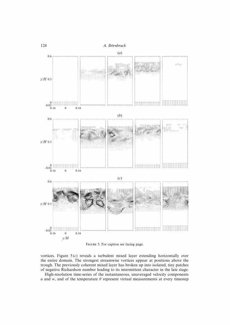
The development of streamwise vortices is displayed in figure 5 by a series of lateralcross-sections of the (v, w)-velocities and the local Richardson number Ri at fivehorizontal locations xα (α = 1, . . . , 5). Early on, the overturning creates an elongatedconvectively unstable layer that is seen as a laterally coherent layer of negative Ri(t = 21.5 in figure 5 a). Its vertical depth depends on x and does not exceed 0.2H .Above the crest (x5 = λ), this layer appears as an elevated, vertically compressedbut laterally essentially homogeneous region. Only weak wave-like disturbances andisolated patches of Ri < 0 (due to the eruptive breaking at earlier times) disturbthe lateral homogeneity. Downstream, the region of instability thickens and descends(see x3 = 0.6 λ and x4 = 0.8 λ). In this layer, the shear vanishes and the amplitudesof the three-dimensional velocity components grow rapidly in time. In this way,the lateral homogeneity is no longer sustained and the downward motion of liftedcold fluid leads to adjacent regions of negative and positive vertical velocity andfinally to the generation of a pair of counter-rotating vortices. The production ofstreamwise vorticity is spatially restricted to the locations inside the convective layer(see positions x2, x3, and x4 at t = 21.5 and 28.5). Hence, the mechanism of generatingstreamwise vortices is dominated by buoyancy at this stage of flow evolution. Theresulting vortices are aligned in the direction of mean shear and wave propagation.Their magnitude is small compared to that of the spanwise overturning rolls.

At t = 28.5, the streamwise vortices have been advected downstream (figure 5 b).The most interesting process occurs near x2 = 0.4 λ where the streamwise vorticesenter a region of strong vertical transport of horizontal momentum. At this location,overturning rolls entrain high-momentum fluid from below (as discussed in figure 2 fort = 32). The penetration through this momentum-flux barrier retards the horizontalexpansion of the mixed region. Vertical components of the flow field are producedresulting in a lifting of the mixed layer (figure 5 b). As a result, streamwise vorticityis created and the three-dimensional mixing extends vertically. In contrast to thedownstream advection of counter-rotating streamwise vortices, the wave-inducedadvection below the critical level to the right of the trough transports vortices in theopposite direction. Above the crest (see positions x4 and x5), these vortices narrowand the vertical extent of the unstable layer is significantly reduced.

At later times (see t = 41.5, figure 5 c), the vertical shear over the crest and atthe lower edge of the mixed layer is the main mechanism for generating streamwise

124 A. Dornbrack

(a)0.6

0.3

0–0.03

0.16 0 0.16

z /H

(b)0.6

0.3

0–0.03

0.16 0 0.16

z /H

(c)0.6

0.3

0–0.03

0.16 0 0.16

z /H

y /H


vortices. Figure 5 (c) reveals a turbulent mixed layer extending horizontally overthe entire domain. The strongest streamwise vortices appear at positions above thetrough. The previously coherent mixed layer has broken up into isolated, tiny patchesof negative Richardson number leading to its intermittent character in the late stage.

High-resolution time-series of the instantaneous, unaveraged velocity componentsu and w, and of the temperature θ represent virtual measurements at every timestep


(a)0.6

0.3

0–0.03

0.16 0 0.16

z /H

(b)0.6

0.3

0–0.03

0.16 0 0.16

z /H

(c)0.6

0.3

0–0.03

0.16 0 0.16

z /H

y /H

Figure 5. Instantaneous velocity field (v, w) (left) and local Richardson number Ri (right) inspanwise sections at xα = 0.2λ, 0.4λ, 0.6λ, 0.8λ and λ (from left to right) at (a) t = 21.5, (b) t = 28.5,(c) t = 41.5. The green contour line indicates Ri = 0, the dashed one Ri = 0.25, and the red linesdenote negative Ri.

126 A. Dornbrack

(a)0.05

0

–0.05

–0.10

u

DU

0 10 20 30 40 50 60 70

0.050

0.025

–0.025

–0.050

w

DU

0 10 20 30 40 50 60 70

0

0.10

0.05

–0.05

–0.150 10 20 30 40 50 60 70

0

–0.10

0.15

t /tref

0.15

0.100.05

0

–0.05–0.10

–0.1516.0 16.5 17.0 17.5 18.0


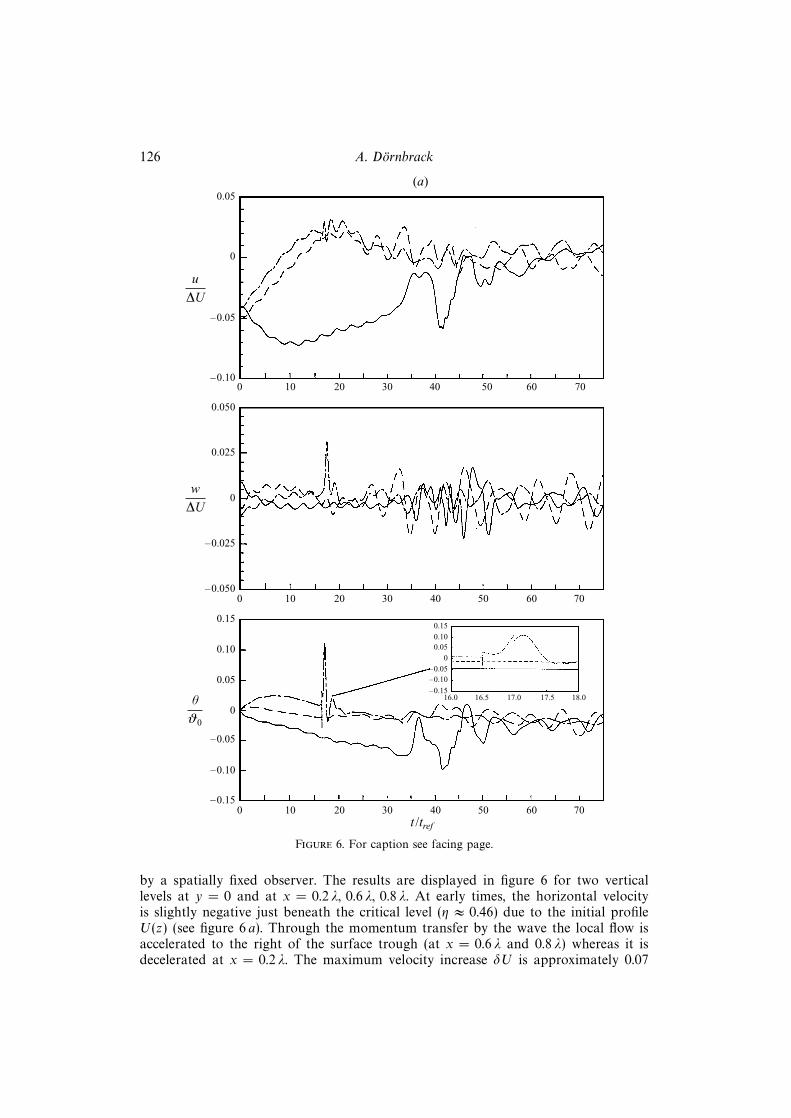
by a spatially fixed observer. The results are displayed in figure 6 for two verticallevels at y = 0 and at x = 0.2 λ, 0.6 λ, 0.8 λ. At early times, the horizontal velocityis slightly negative just beneath the critical level (η ≈ 0.46) due to the initial profileU(z) (see figure 6 a). Through the momentum transfer by the wave the local flow isaccelerated to the right of the surface trough (at x = 0.6 λ and 0.8 λ) whereas it isdecelerated at x = 0.2 λ. The maximum velocity increase δU is approximately 0.07


(b)–0.15

–0.20

–0.25

–0.30

u

DU

0 10 20 30 40 50 60 70

0.050

0.025

–0.025

–0.050

w

DU

0 10 20 30 40 50 60 70

0

0.05

–0.050 10 20 30 40 50 60 70

0

0.10

t /tref

Figure 6. (a) Time-series of local and instantaneous values of the streamwise and vertical velocityu and w, and of the temperature θ. Data are taken every timestep of the numerical model at threex-positions in the plane y = 0 and at η ≈ 0.46. The respective z-positions of the three curves arex/λ = 0.2: ———– at z = 0.462; x/λ = 0.6: – – – – at z = 0.4894; x/λ = 0.8: – · – · – at z = 0.462.(b) As (a) but for η ≈ 0.21: x/λ = 0.2: ———– at z = 0.232; x/λ = 0.6: – – – – at z = 0.205;x/λ = 0.8: – · – · – at z = 0.232.

128 A. Dornbrack

at this vertical level. It reaches larger values at lower altitudes, up to δU = 0.12 atη ≈ 0.38. At t ≈ 10, the horizontal velocity at x = 0.2 λ also increases because theregion of strong vertical transport of horizontal momentum has been shifted in thenegative x-direction. At the same horizontal position, u undergoes large-amplitudeoscillations during the period (t ≈ 35–50) when the momentum-flux barrier has beenpenetrated by streamwise vortices and turbulence production has become maximumunderneath. Similar temporal oscillations occur in the thermal field: strong negativetemperature fluctuations arise simultaneously with large u-values indicating the small-scale shear-induced secondary overturning rolls. In the late stage, the u-time-series atthis vertical level show wave-like oscillations around the level u = 0 caused by theadvection of overturning rolls at lower altitudes. The most distinct signal in the w-and θ-fields is the strong oscillation in the primary unstable layer (x = 0.8 λ) due tothe convective instability. Figure 6 (a) also displays an abrupt temperature change att = 16.5 due to the spontaneous and explosive breaking. Afterwards, the temperaturefluctuation increases rapidly but smoothly. However, it is disrupted again at t = 17by another eruption from the convectively unstable flow. The vertical velocity fieldchanges smoothly and follows the temperature field temporally. At later times, thelarge-amplitude oscillations caused by the breaking are damped but are excited againwhen turbulence is produced at lower levels.

In contrast to η ≈ 0.46, the time series at lower altitude η ≈ 0.21 show turbulenceafter a wavy period lasting up to t ≈ 35 (see figure 6 b). In the following, the discussionwill be confined to the curve x = 0.2 λ because the other horizontal positions behavesimilarly. Initially, the local velocity u is negative (u ≈ −0.27). The smaller deposit ofwave momentum causes a smaller rate of velocity change at this level compared toη ≈ 0.46. During the early stage, periodic oscillations with a nearly constant periodT ≈ 3.1 or a frequency of ω = 2 appear as the dominant signal in all curves. For a fluidat rest, the maximum frequency allowed for internal gravity waves is the Brunt–Vaisala

frequency N = Ri1/2B ≈ 1. However, at the bottom surface, perturbations of frequency

kxU ≈ 2 are excited as seen in the time-series. Therefore, the observed frequencyis just twice N. The intrinsic frequency of the gravity waves is ω = ω − kxu(η). Atη ≈ 0.21 and for all heights where γ < 1, ω is less than N, as expected. The amplitudeof the velocity and temperature oscillations is large compared to the level η ≈ 0.46.Interestingly, the magnitude of the temperature amplitude alternates periodically intime up to t = 20 (see figure 6 b). The period between the respective maxima isapproximately 6. If we take a mean velocity U0 = −0.26 at this level and if we assumethat the whole flow structures remain unchanged in time, then they return at a fixedposition every λ/U0 = 1.5625 /0.26 ≈ 6. Hence, the origin of these returning patternsis simply their advection by the mean flow. During the breaking, the time-seriesare characterized by intermittent high-frequency oscillations and smooth (laminar)periods. The occurrence of the turbulent periods is caused by the isolated regions ofnegative Richardson number in the cores of the overturning rolls.

4. Reynolds number influenceIn Dornbrack et al. (1995) it was shown that for sufficient viscous damping three-

dimensional turbulent convective instabilities are more easily suppressed than two-di-mensional overturning. Using only constant diffusivities instead of the subgrid-scalemodel of (2.7), no turbulent motions were found. Mixing takes place as a quasi-periodic rolling-up of isentropes and the flow permanently contains overturning rolls.On the other hand, in runs where νM = 0 and νturb 6= 0, overturning waves immediately


t = 480.56

0

0.28

–0.030 0.78 1.56

x/H0 0.78 1.56

x/H

t = 440.56

0

0.28

–0.03

t = 320.56

0

0.28

–0.03

t = 200.56

0

0.28

–0.03

t = 80.56

0

0.28

–0.03

z

H

(a) (b)

z

H

z

H

z

H

z

H

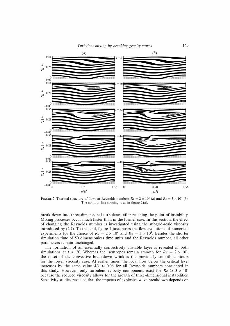
Figure 7. Thermal structure of flows at Reynolds numbers Re = 2× 104 (a) and Re = 3× 104 (b).The contour line spacing is as in figure 2 (a).

break down into three-dimensional turbulence after reaching the point of instability.Mixing processes occur much faster than in the former case. In this section, the effectof changing the Reynolds number is investigated using the subgrid-scale viscosityintroduced by (2.7). To this end, figure 7 juxtaposes the flow evolutions of numericalexperiments for the choice of Re = 2 × 104 and Re = 3 × 104. Besides the shortersimulation time of 50 dimensionless time units and the Reynolds number, all otherparameters remain unchanged.

The formation of an essentially convectively unstable layer is revealed in bothsimulations at t ≈ 20. Whereas the isentropes remain smooth for Re = 2 × 104,the onset of the convective breakdown wrinkles the previously smooth contoursfor the lower viscosity case. At earlier times, the local flow below the critical levelincreases by the same value δU ≈ 0.06 for all Reynolds numbers considered inthis study. However, only turbulent velocity components exist for Re > 3 × 104

because the reduced viscosity allows for the growth of three-dimensional instabilities.Sensitivity studies revealed that the impetus of explosive wave breakdown depends on

130 A. Dornbrack

20 40 60 800

20 40 60 800

2

4

6

(b)

2

4

6

(a)

t /tref

νturb

νM (%)

νturb

νM (%)

Figure 8. Temporal evolution of the ratio νturb/νM for (a) Re = 5 · 104 and (b) Re = 3 × 104.The curves are averages over horizontal planes of constant η = 0.35 (———–), 0.39 (- - - - - -), 0.42(– · – · –), 0.45 (– · · · – · · · –), 0.47 (— — —).

the Prandtl number: temperature fluctuations initiated by the convective breakdownbecome larger as a result of a reduced thermal conductivity 1/RePr.

At later times (t > 20), the flow remains essentially two-dimensional for higherviscosity and approaches an equilibrium state where the convectively unstable re-gion is maintained without turbulence production. This structure resembles the two-dimensional findings of Winters & d’Asaro (1989) who observed that wave overturn-ing persists for more than ten buoyancy periods without breaking. The low-viscositycase produces a horizontally extended turbulent mixed layer as described for caseRe = 5× 104 in § 3. Note, that the acceleration for positions to the left of the trough(x < λ/2) depends strongly on Re. For Re = 5× 104 the local flow accelerates up toδU ≈ 0.22 whereas for Re = 2× 104 it reaches only δU ≈ 0.12 at t = 45. Hence, thelower the viscosity, the higher the momentum transfer to the local mean flow and,finally, the earlier the breakdown and the transition to a turbulent mixed layer.

The flow-independent part νM dominates the total viscosity as shown in figure 8.There, the ratio of horizontally averaged turbulent to kinematic viscosity νturb/νMis shown for Re = 3 × 104 and 5 × 104 at selected altitudes up to the critical level.Although the ratio is much smaller for Re = 3 × 104 compared to Re = 5 × 104,their temporal behaviours are similar. The turbulent viscosity νturb is different fromzero only when the local Richardson number drops below the critical value andif the shear perturbation S ′ has grown in the region below the critical level. Theretarded increase of the ratio at different vertical levels shows the downward spreadof the mixed region. The ratio νturb/νM never exceeds 6%, i.e. the additional turbulentcontribution enhances the total viscosity only slightly. However, during a breakingevent, instantaneous values of νturb attain 20% to 30% of νM . These are restricted to


(a) η = 0.05

–4

–6

–8

–1030010030103

(b) η = 0.35

–4

–6

–8

–1030010030103

(b) η = 0.47

–4

–6

–8

–1030010030103

Re =

2 ×104

–4

–6

–8

–1030010030103

–4

–6

–8

–1030010030103

–4

–6

–8

–1030010030103

3 ×104

–4

–6

–8

–1030010030103

–4

–6

–8

–1030010030103

–4

–6

–8

–1030010030103

5 ×104

k k k

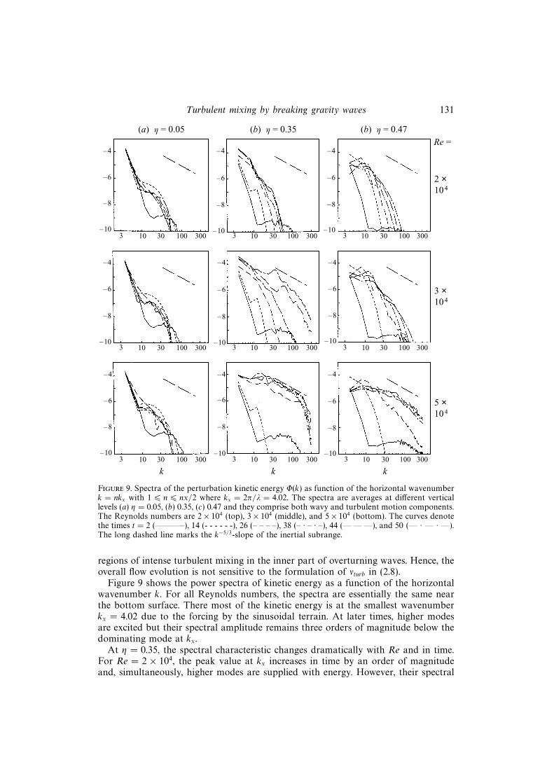
Figure 9. Spectra of the perturbation kinetic energy Φ(k) as function of the horizontal wavenumberk = nkx with 1 6 n 6 nx/2 where kx = 2π/λ = 4.02. The spectra are averages at different verticallevels (a) η = 0.05, (b) 0.35, (c) 0.47 and they comprise both wavy and turbulent motion components.The Reynolds numbers are 2× 104 (top), 3× 104 (middle), and 5× 104 (bottom). The curves denotethe times t = 2 (———–), 14 (- - - - - -), 26 (– – – –), 38 (– · – · –), 44 (— — —), and 50 (— · — · —).The long dashed line marks the k−5/3-slope of the inertial subrange.

regions of intense turbulent mixing in the inner part of overturning waves. Hence, theoverall flow evolution is not sensitive to the formulation of νturb in (2.8).

Figure 9 shows the power spectra of kinetic energy as a function of the horizontalwavenumber k. For all Reynolds numbers, the spectra are essentially the same nearthe bottom surface. There most of the kinetic energy is at the smallest wavenumberkx = 4.02 due to the forcing by the sinusoidal terrain. At later times, higher modesare excited but their spectral amplitude remains three orders of magnitude below thedominating mode at kx.

At η = 0.35, the spectral characteristic changes dramatically with Re and in time.For Re = 2 × 104, the peak value at kx increases in time by an order of magnitudeand, simultaneously, higher modes are supplied with energy. However, their spectral

132 A. Dornbrack

amplitude remains negligibly small compared to that of kx. The temporal change ofΦ(k) for Re = 3 × 104 reveals a gradual energy injection at smaller scales so thatthe dominant scale of disturbances is larger than 0.2 λ. In the period t = 44–50,the spectral energy grows rapidly at small scales due to small-scale overturning andturbulence.

A dramatic increase in the energy for wavenumbers larger than k ≈ 10 (or wave-lengths less than 0.4 λ) characterizes the spectra for Re = 5 × 104 during the periodt = 14–26. For t > 38, a classical turbulence profile is obtained at this verticallevel: most of the kinetic energy is contained in scales between 0.15 λ and 0.35 λ(k ≈ 10–30). This scale roughly corresponds to the diameter of the energetic secondaryrolls. The spectral amplitude of Φ(k) slopes according to k−5/3 for the wavenumber30 < k < 200 (scales down to 0.02 λ). For smaller scales (k > 200), dissipationdominates the k−x-slope, where x > 7. The turbulent Reynolds number is defined asReturb = (Lturb/ηturb)

4/3. In the mixed layer the integral scale Lturb and the microscaleηturb of turbulence can be estimated from the spectra in figure 9. Lturb is the scaleof energy injection into the inertial subrange (≈ 0.2 λ) and ηturb ≈ 0.016 λ is thescale where Φ(k) becomes proportional to k−7, i.e. the turbulent Reynolds number ofthe flow is estimated to be Returb ≈ 30. Subsequently, the dissipation range expandstowards smaller wavenumbers (up to k = 100) while the large-scale peak of the in-ertial subrange remains at k ≈ 10–30. Consequently, the turbulent Reynolds numberdecreases to Returb ≈ 10 during the latter stage of flow evolution.

In order to complete the picture, Φ(k)-spectra on the plane η = 0.47 are displayedin figure 9(c). Initially, this plane is located directly beneath the critical level. For timeswhen the critical level has descended below η = 0.47, spectral amplitude decreases.The spectra are similarly shaped but their amplitude is about an order of magnitudesmaller compared to those at the lower level η = 0.35.

5. Energetics and mixing efficiencyThe budgets of domain-averaged total energy per unit mass ET and of turbulent

kinetic energy E ′′K for case Re = 5× 104 were computed. At t = 0, the total potentialenergy is set to zero and only deviations in E ′P from this equilibrium state areconsidered. Then, the total initial energy can be estimated by the kinetic energy fromthe prescribed velocity field U(z) alone:

ET (0) = EK(0) ≈ 1

2

∫ 1

0

U2(z) dz =1

2

∫ 1

0

(z − 0.5)2, dz =1

24. (5.1)

For t > 0, the total kinetic energy per unit mass EK = 0.5V

u2i (

V

f(t) denotes thedomain average of a quantity f) can be divided into three parts according to (A 3)in the Appendix: EK = EM

K + EK + E ′′K , where the mean kinetic energy EMK and the

wavy and turbulent parts are calculated by means of

EMK = 1

2

V

ui2, EK = 1

2

V

ui2, E ′′K = 1

2

V

u′′2, (5.2)

where E ′K = EK + E ′′K . By analogy, the potential energy perturbation E ′P can be

divided into available potential energy EP = 12RiB

V

ϑ2 and into the potential energy

E ′′P = 12RiB

V

ϑ′′2 associated with turbulent mixing. Table 1 lists instantaneous values

of EMK , E ′K , E ′P and of the accumulated energy loss by mechanical dissipation L. The


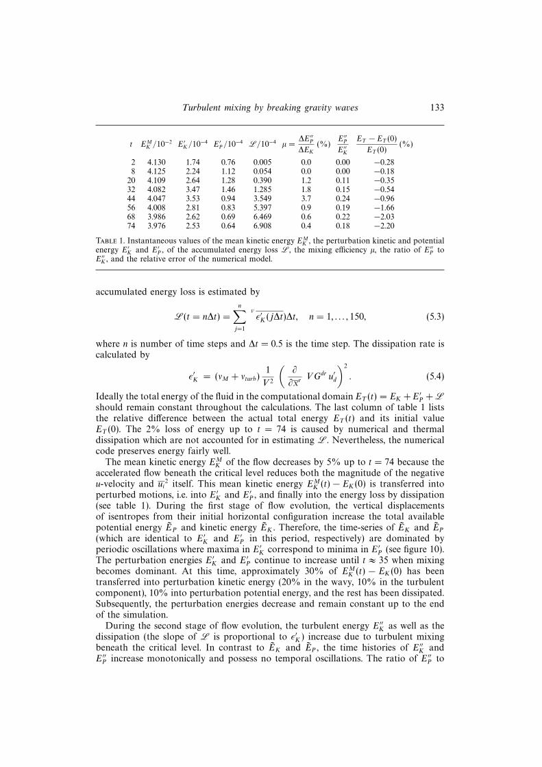
t EMK /10−2 E ′K/10−4 E ′P /10−4 L/10−4 µ =

∆E ′′P∆EK

(%)E ′′PE ′′K

ET − ET (0)

ET (0)(%)

2 4.130 1.74 0.76 0.005 0.0 0.00 −0.288 4.125 2.24 1.12 0.054 0.0 0.00 −0.18

20 4.109 2.64 1.28 0.390 1.2 0.11 −0.3532 4.082 3.47 1.46 1.285 1.8 0.15 −0.5444 4.047 3.53 0.94 3.549 3.7 0.24 −0.9656 4.008 2.81 0.83 5.397 0.9 0.19 −1.6668 3.986 2.62 0.69 6.469 0.6 0.22 −2.0374 3.976 2.53 0.64 6.908 0.4 0.18 −2.20

Table 1. Instantaneous values of the mean kinetic energy EMK , the perturbation kinetic and potential

energy E ′K and E ′P , of the accumulated energy loss L, the mixing efficiency µ, the ratio of E ′′P toE ′′K , and the relative error of the numerical model.

accumulated energy loss is estimated by

L(t = n∆t) =

n∑j=1

V

ε′K(j∆t)∆t, n = 1, . . . , 150, (5.3)

where n is number of time steps and ∆t = 0.5 is the time step. The dissipation rate iscalculated by

ε′K = (νM + νturb)1

V 2

(∂

∂xrVGdr u′d

)2

. (5.4)

Ideally the total energy of the fluid in the computational domain ET (t) = EK +E ′P +Lshould remain constant throughout the calculations. The last column of table 1 liststhe relative difference between the actual total energy ET (t) and its initial valueET (0). The 2% loss of energy up to t = 74 is caused by numerical and thermaldissipation which are not accounted for in estimating L. Nevertheless, the numericalcode preserves energy fairly well.

The mean kinetic energy EMK of the flow decreases by 5% up to t = 74 because the

accelerated flow beneath the critical level reduces both the magnitude of the negativeu-velocity and ui

2 itself. This mean kinetic energy EMK (t) − EK(0) is transferred into

perturbed motions, i.e. into E ′K and E ′P , and finally into the energy loss by dissipation(see table 1). During the first stage of flow evolution, the vertical displacementsof isentropes from their initial horizontal configuration increase the total availablepotential energy EP and kinetic energy EK . Therefore, the time-series of EK and EP(which are identical to E ′K and E ′P in this period, respectively) are dominated byperiodic oscillations where maxima in E ′K correspond to minima in E ′P (see figure 10).The perturbation energies E ′K and E ′P continue to increase until t ≈ 35 when mixingbecomes dominant. At this time, approximately 30% of EM

K (t) − EK(0) has beentransferred into perturbation kinetic energy (20% in the wavy, 10% in the turbulentcomponent), 10% into perturbation potential energy, and the rest has been dissipated.Subsequently, the perturbation energies decrease and remain constant up to the endof the simulation.

During the second stage of flow evolution, the turbulent energy E ′′K as well as thedissipation (the slope of L is proportional to ε′K) increase due to turbulent mixingbeneath the critical level. In contrast to EK and EP , the time histories of E ′′K andE ′′P increase monotonically and possess no temporal oscillations. The ratio of E ′′P to

134 A. Dornbrack

8

6

4

2

0 20 40 60 80

t /tref

Ene

rgy

(× 1

0–4

) ,

E ′K

EK

E ′′K

E ′′P

E ′P

EP

Figure 10. Time-series of volume-averaged perturbation kinetic and potential energies E ′K = EK+E ′′Kand E ′P = EP +E ′′P for Re = 5× 104. The wavy motion components are marked by dotted lines, theturbulent components by dashed lines. The accumulated loss of kinetic energy through mechanicaldissipation is denoted by L.

the turbulent kinetic energy E ′′K becomes maximum 24% during the intense mixingperiod (see table 1).

The potential energy E ′′P increases because turbulent mixing takes place beneaththe critical level. The ratio of the potential energy increase ∆E ′′P to the kinetic energyloss ∆EK during the mixing event determines the mixing efficiency µ, i.e. the amountof mean kinetic energy that has been spent to modify the basic-state stratificationirreversibly. The kinetic energy loss during the breaking period is estimated by∆EK = EK(t)−EK(0). As expected, the mixing efficiency is zero during the first stage(up to t ≈ 17) when only wave-like motions exist in the fluid. When wave breakingoccurs, µ increases up to 4%. This implies that just this amount of mean kineticenergy is released to increase the potential energy.

The budget of the domain-averaged turbulent kinetic energy (TKE) reads

∂

∂tE ′′K + ADV = SP + BP + DIFF− ε, (5.5)

where ADV, SP, BP, DIFF and ε denote the advection, the shear production, thebuoyancy production, the diffusion, and the dissipation, respectively:

ADV =1

V

V

∂

∂xd(VGdjujE

′′K

),

DIFF =1

V

V

∂

∂xd(GdjVJj

)where Jj =

V

u′′j(E ′′K + p′′/ρ0

),

SP = −u′′i u′′j1

V

V

∂

∂xd(VGdjuj

),

BP = RiBV

w′′θ′′,

ε = (νturb + νM)1

V 2

V

∂

∂xr(VGdru′′d

)2.

(5.6)

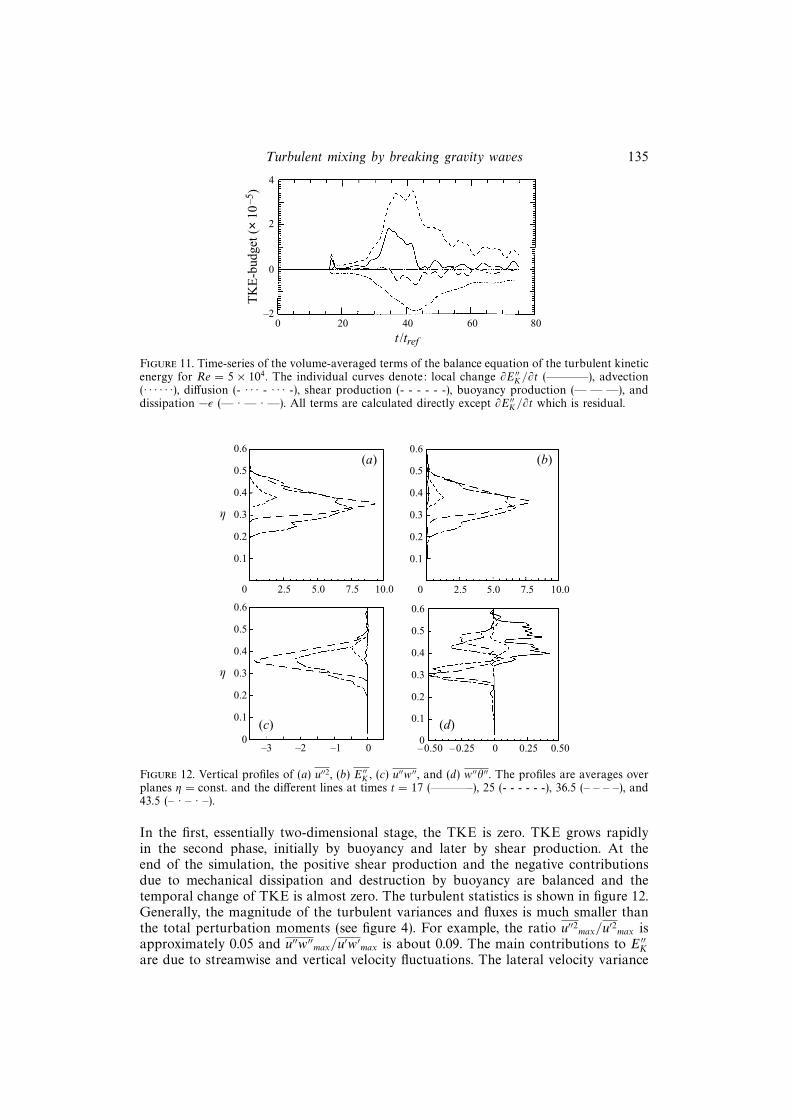
Time-series of the individual terms of (5.5) are plotted in figure 11. Except for theresidual determination of (∂/∂t)E ′′K , all other terms are calculated directly accordingto (5.6). As expected, advection and diffusion equal zero. In terms of TKE and inaccordance with results of § 3, the flow regime can be characterized in three stages.


4

2

0

–20 20 40 60 80

t /tref

TK

E-b

udge

t (×

10–5

)

Figure 11. Time-series of the volume-averaged terms of the balance equation of the turbulent kineticenergy for Re = 5 × 104. The individual curves denote: local change ∂E ′′K/∂t (———–), advection(· · · · · ·), diffusion (- · · · - · · · -), shear production (- - - - - -), buoyancy production (— — —), anddissipation −ε (— · — · —). All terms are calculated directly except ∂E ′′K/∂t which is residual.

(a)0.6

0.5

0.4

0.3

0.2

0.1

0 2.5 5.0 7.5 10.0

η

(b)0.6

0.5

0.4

0.3

0.2

0.1

0 2.5 5.0 7.5 10.0

(c)

0.6

0.5

0.4

0.3

0.2

0.1

0–3 –2 –1 0

η

(d)

0.6

0.5

0.4

0.3

0.2

0.1

0–0.50 0 0.25 0.50–0.25

Figure 12. Vertical profiles of (a) u′′2, (b) E ′′K , (c) u′′w′′, and (d) w′′θ′′. The profiles are averages overplanes η = const. and the different lines at times t = 17 (———–), 25 (- - - - - -), 36.5 (– – – –), and43.5 (– · – · –).

In the first, essentially two-dimensional stage, the TKE is zero. TKE grows rapidlyin the second phase, initially by buoyancy and later by shear production. At theend of the simulation, the positive shear production and the negative contributionsdue to mechanical dissipation and destruction by buoyancy are balanced and thetemporal change of TKE is almost zero. The turbulent statistics is shown in figure 12.Generally, the magnitude of the turbulent variances and fluxes is much smaller thanthe total perturbation moments (see figure 4). For example, the ratio u′′2max/u′2max isapproximately 0.05 and u′′w′′max/u′w′max is about 0.09. The main contributions to E ′′Kare due to streamwise and vertical velocity fluctuations. The lateral velocity variance

136 A. Dornbrack

(a) η = 0.470.00002

–0.00001

0

0.00001

30010030103

(b) η = 0.39

0.00001

–0.00003

0

30010030103

–0.00002

–0.00001

(c) η = 0.430.00002

–0.00001

0

0.00001

30010030103

(d ) η = 0.35

0.00001

–0.00003

0

30010030103

–0.00002

–0.00001

k k

Figure 13. Co-spectra of the vertical heat flux Φw′θ′ (k) in an early (a, c) and a late period (b, d) ofwave breaking. As in figure 9, the individual curves are averages over planes η = const. The linesare for different times: ———: 16.5 (a, c), 44 (b, d); - - - - - -: 17 (a, c), 50 (b, d); – – – –: 17.5 (a, c),56 (b, d); – · – · –: 18 (a, c), 62 (b, d).

v′′2 ≈ v′2 is approximately a factor 2 smaller than u′′2. The turbulent momentum fluxis always negative and counteracts the positive flux of the wave motion. This leads toa reduction of the total momentum flux down to about z = 0.2 as shown in figure 4.

The vertical turbulent heat flux is always negative except during the early stage ofwave breaking. A negative heat flux implies that (on average) upward motions causecooling and downward motions heating. In a thermally stably stratified environment,a positive heat flux is counter-gradient to the mean temperature gradient dϑ/dz.

However, this flux occurs initially in a vertically limited layer of negative dϑ/dz,

hence −w′′θ′′ is aligned with the mean temperature gradient and downgradient. Asthe Φw′θ′-spectra show pronounced maxima at high wavenumbers, small-scale motionsmust be responsible for the occurrence of positive w′′θ′′ (see figure 13 a,b). Note thatthe spectra Φw′θ′ comprehend both wavy and turbulent velocity components. However,their dominating modes are spectrally separated at this stage. The contributions of thewavy components are at small wavenumbers and appear either positive or negativedepending on the respective vertical level and time. Figure 13 (c,d) shows Φw′θ′-spectrain the turbulent stage of flow evolution. There, the spectra are taken from loweraltitudes than those in figure 13 (a,b). Averaged over all wavenumbers, the heatflux w′θ′ is negative. The main contribution to this flux stems from overturningrolls at wavenumbers between k = 10 and 30. The pronounced minima of Φw′θ′


appear at the same horizontal wavenumber as the maximum of Φ(k). Although thespectra show a positive maxima at k ≈ 30, the turbulent contributions occurringat higher wavenumbers are nearly zero in the inertial subrange. Thus, the largeeddies (overturning rolls), which are resolved in the simulation, are very efficient indowngradient transport of heat.

6. Discussion and conclusionsThe three-dimensional breaking of internal gravity waves beneath a critical level

has been investigated by means of high-resolution numerical simulations. For thispurpose, the flow evolution of a stably stratified Boussinesq fluid confined between awavy bottom and a plane top surface, both frictionless and adiabatic, was studied. Theparameters used in the model are similar to those of Thorpe’s (1981) tank experiment.

The simulation of the transition from two-dimensional wave motions to three-dimensional turbulence requires a fine spatial resolution in regions of wave insta-bility. Therefore, the incompressible finite difference scheme using terrain-followingcoordinates (Krettenauer & Schumann 1992) was improved by increasing the verticalresolution near the critical level (see (2.4)). Moreover, the subgrid-scale viscosities KM

and KH were modelled by the sum of a uniform and a flow-dependent part accordingto (2.7). Various Reynolds numbers have been tested to find the highest Re for whichthe simulation results become insensitive to further Re-changes and which minimallydamp the energy at small scales. For the detailed study of the turbulent breakdownof overturning internal gravity waves Re ≈ 5× 104 was chosen.

What are the details of breaking?

The simulated flow evolution occurs in three stages. During the first stage, the flowremains two-dimensional. The flow over the fixed wavy surface induces stationarygravity waves with respect to topography. Above the critical level, no or very small-amplitude damped wavy disturbances are observed. Below the critical level, the maineffect is the persistent acceleration of the mean flow in the positive x-direction. Thisacceleration is opposite to the direction of U(z) for z < 0.5. The perturbed meanflow lifts heavier fluid over lighter fluid directly beneath the critical level, whereasthe mean advection in the negative x-direction at lower altitudes moves lighter fluidunder heavier. Between these levels, the fluid stagnates and a convectively unstableregion is formed that extends over almost one wavelength λ and has a thickness ofabout 0.1 the layer depth.

During the second stage, explosive convective instability leads to the first turbulentbreakdown. Approximately three Brunt–Vaisala periods are required for the devel-opment of three-dimensional motions. The developing mixed layer is organized inspanwise, shear-driven overturning rolls and in counter-rotating streamwise vortices.At first, streamwise vortices derive their energy mainly from buoyancy; later sheardominates. The temporal order of instabilities found in this study agrees with pre-dictions from linear perturbation theories by Winters & Riley (1992) and by Linet al. (1993) and with numerical results of Winters & d’Asaro (1994). In contrast,Scinocca (1995) found that shear instability occurs before convective instability formixed layers produced in overturning Kelvin–Helmholtz billows. The present resultsconfirm Schowalter, Van Atta & Lasheras’s (1994) finding that buoyancy forces con-tribute to an additional mechanism for the generation of streamwise vortices in thepresence of stratification.

138 A. Dornbrack

The flow in the mixed layer is random, containing vortices on a wide range ofscales. The typical horizontal scale of a spanwise secondary roll is 0.2λ–0.3 λ; the scaleof the streamwise vortices is less than 0.15 λ. Caulfield & Peltier (1994) investigatingstratified shear layers also found the scale of streamwise streaks of vorticity to be muchsmaller than the wavelength of the primary overturning structures. The lateral scale ofcounter-rotating streamwise vortices is smaller than the width of the computationaldomain and their size appears to be unaffected by it.

The final stage of flow evolution is characterized by a quasi-steady equilibriumbetween shear production and mechanical dissipation of turbulent kinetic energy. Thefinal mixed layer consists of shear-induced, small-scale overturning rolls and counter-rotating streamwise vortices leading to isolated patches of turbulence embedded in asmooth flow.

What is the role of viscosity?

The results of § 4 have shown that (i) the smaller νM is, the earlier breaking occurs inthe convectively unstably stratified regions. The flow becomes fully three-dimensional.Secondly, the smaller the viscosity, the larger the momentum deposited beneath thecritical level by gravity waves and the more likely is the formation of secondary rollsand turbulent breaking by shear instability. These findings agree with results of Frittset al. (1996) who found viscosity retarding instability.

What are the characteristics of turbulence generated by breaking gravity waves?

Turbulence is primarily produced by shear in the mixed layer. There, the powerspectra of perturbation kinetic energy resemble classical spectra from turbulencetheory. The spectral amplitude slopes according to k−5/3 for scales smaller 0.2 λ anddown to 0.02 λ. For scales less than 0.02 λ, the spectral amplitude decreases accordingto k−x, where x > 7 (dissipation range). Based on estimates of the integral scaleand microscale of turbulence, the turbulent Reynolds number is computed to beapproximately 30. Another remarkable result is the apparent sinking of the mixedlayer due to entrainment of cold and high-momentum fluid at its lower edge. Sinkingof thin turbulent layers has also been observed by radar in the free atmosphere (Sato& Woodman 1982).

How much energy of the mean flow is transferred to waves, how much to turbulence?

Although the separation into wavy and turbulent parts is controversial (see Hol-loway 1988; Winters et al. 1995), it does aid in determining the essential sources ofinstability energy. The mean kinetic energy of the flow decreases temporally by 5%up to t = 74. This mean kinetic energy is converted into perturbation kinetic andpotential energy. Finally it is lost by dissipation. By the time that the flow reachesits quasi steady-state, approximately 30% of this energy has become perturbationkinetic energy (20% in the wavy, 10% in the turbulent component), 10% has becomeperturbation potential energy, and the remainder has been dissipated. As a checkof numerical accuracy, the budget of the total kinetic energy has been computed;approximately 2% of the total energy was lost by thermal dissipation and by nu-merical diffusion. For internal gravity waves, the relevant dissipation process is theirunstable breakdown via convective and dynamical instabilities. The mixing efficiencywas calculated to be approximately 4%. Thus this small amount of mean kineticenergy is converted to potential energy and into an irreversible change of the initialthermal stratification.


Although Winters & d’Asaro (1994) and Fritts et al. (1996) investigated similarproblems to ours, their numerical approaches (integration method, background con-ditions, wave forcing, and subgrid-scale modelling) are different. Winters & d’Asaro(1994), using a pseudospectral method, investigated the overturning of an initially pre-scribed, two-dimensional internal wave packet in an incompressible Boussinesq fluid.The ambient flow possessed constant stability and a depth-dependent shear flow witha critical level in the essentially linear segment of U(z). The bulk Richardson numberof 25 is higher and the spatial resolution lower compared to the present simulations.Furthermore, the classic diffusion operator was replaced by a sixth-order derivative.Fritts et al. (1996) investigated and compared the two- and three-dimensional break-ing by integrating the compressible Eulerian equations using a spectral collocationmethod. Specifically, the instability structure subject to shear components transverseto the direction of wave propagation was investigated. The gravity waves were forcedby a time-dependent body force that yields a wave packet containing many differentfrequencies and vertical wavenumbers. The viscous and diffusive effects are repre-sented spectrally by a method described by Andreassen et al. (1994). In order toachieve a finer resolution at the locations of instability, Fritts et al. (1996) decom-posed the model vertically into two domains and Winters & d’Asaro (1994) used upto 200 vertical levels. The instability growth and the structures of the breaking wavesin this study agree fairly well with these other different numerical approaches.

This work was funded by the Deutsche Forschungsgemeinschaft (DFG) in theframework of the Schwerpunktprogramm “Grundlagen der Auswirkungen der Luft-und Raumfahrt auf die Atmosphare”.

AppendixThe classical Reynolds decomposition splits an arbritrary field f into a mean part

f and a fluctuating part f′ according to f = f + f′. Usually, in numerical studies,the mean part of the discrete field fi,j,k(t) is defined as average over horizontal planesaccording to

fk(z, t) =1

nx ny

nx,ny∑i,j=1

fi,j,k(t). (A 1)

Additionally, temporal averages can be used when the flow has reached a steady state.In the present study, the fluctuating part f′ is split diagnostically into a wavy (f) anda turbulent (f′′) component. A phase average (here, just over one wavelength)

〈f〉p(x, z, t) =1

ny

ny∑j=1

fi,j,k(t) (A 2)

can be used to extract the wavy component f from f according to f(x, η, t) = 〈f〉p−f.This sort of averaging is appropriate as long as the gravity wave excitation ishomogeneous in y and the resulting flow structures are shorter than λ. Finally, thetotal field f consists in a mean part f, a wavy (f), and a turbulent (f′′) part accordingto

f = f + f + f′′ where f′′(x, y, z, t) = f − f − f. (A 3)

This sort of decomposition was introduced by Hussain & Reynolds (1970) andhas been formerly used inter alia by Fritts, Isler & Andreassen (1994) and Frittset al. (1996).

140 A. Dornbrack

REFERENCES

Andreassen, Ø., Wasberg, C. E., Fritts, D. C. & Isler, J. R. 1994 Gravity breaking in twoand three dimensions. 1. Model description and comparison of two-dimensional evolutions.J. Geophys. Res. 99, 8095–8108.

Bacmeister, J. T., Newman, P. A., Gary, B. L. & Chan, K. R. 1994 An algorithm for forcastingmountain wave-related turbulence in the stratosphere. Weather and Forcasting 9, 241–253.

Baines, P. G. 1995 Topographic Effects in Stratified Flows. Cambridge University Press, 482 pp.

Booker, J. R. & Bretherton, F. P. 1967 The critical layer for internal gravity waves in a shearflow. J. Fluid Mech. 27, 513–539.

Broad, A. S. 1995 Linear theory of momentum fluxes in 3-D flows with turning of the mean windwith height. Q. J. R. Met. Soc. 121, 1891–1902.

Carslaw, K. S., Wirth, M., Tsias, A., Luo, B. P., Dornbrack, A., Leutbecher, M., Volkert,

H., Renger, W., Bacmeister, J. T. & Peter, T. 1998a Particle microphysics and chemistry inremotely observed mountain polar stratospheric clouds. J. Geophys. Res. 103, 5785–5796.

Carslaw, K. S., Wirth, M., Tsias, A., Luo, B. P., Dornbrack, A., Leutbecher, M., Volkert, H.,

Renger, W., Bacmeister, J. T., Reimer, E. & Peter, T. 1998b Increased stratospheric ozonedepletion due to mountain-induced atmospheric waves. Nature 391, 675–678.

Caulfield, C. P. & Peltier, W. R. 1994 Three dimensionalization of the stratified mixing layer.Phys. Fluids 6, 3803–3805.

Delisi, D. P. & Dunkerton, T. J. 1989 Laboratory observations of gravity wave critical-layer flows.Pure Appl. Geophys. 130, 445–461.

Dornbrack, A. & Durbeck, T. 1998 Turbulent dispersion of aircraft exhausts in regions of breakinggravity waves. Atmos. Env. 32, 3105–3112.

Dornbrack, A., Gerz, T. & Schumann, U. 1995 Turbulent breaking of overturning gravity wavesbelow a critical level. Appl. Sci. Res. 54, 163–176.

Dornbrack, A. & Nappo, C. J. 1997 A note on the application of linear wave theory at a criticallevel. Boundary Layer Met. 82, 399–416.

Dunkerton, T. J & Robins, R. E. 1992 Radiating and nonradiating modes of secondary instabilityin a gravity-wave critical-level. J. Atmos. Sci. 49, 2546–2559.

Eliassen, A. & Palm, E. 1960 On the transfer of energy in stationary mountain waves. GeofysiskePublikasjoner XXII, 1–23.

Fritts, D. C. 1982 The transient critical-level interaction in a Boussinesq fluid. J. Geophys. Res. 87,7997–8016.

Fritts, D. C., Garten, J. F. & Andreassen, Ø. 1996 Wave breaking and transition to turbulencein stratified shear flows. J. Atmos. Sci. 53, 1057–1085.

Fritts, D. C., Isler, J. R. & Andreassen, Ø. 1994 Gravity breaking in two and three dimensions.2. Three-dimensional evolution and instability structure. J. Geophys. Res. 99, 8109–8123.

Gill, A. E. 1982 Atmosphere-Ocean Dynamics. Academic.

Grubisic, V. & Smolarkiewicz, P. K. 1997 The effect of critical levels on 3D orographic flows:linear regime. J. Atmos. Sci. 54, 1943–1960.

Holloway, G. 1988 The buoyancy flux from internal gravity wave breaking. Dyn. Atmos. Oceans12, 107–125.

Hussain, A. K. M. F. & Reynolds, W. C. 1970 The mechanics of an organized wave in turbulentshear flow. J. Fluid Mech. 41, 241–258.

Kim, Y.-J. & Arakawa, A. 1995 Improvement of orographic gravity wave parametrization using amesoscale gravity wave model. J. Atmos. Sci. 52, 1875–1902.

Koop, C. G. & McGee, B. 1986 Measurements of internal gravity waves in a continiously stratifiedshear flow. J. Fluid Mech. 172, 453–480.

Krettenauer, K. & Schumann, U. 1992 Numerical simulation of turbulent convection over wavyterrain. J. Fluid Mech. 237, 261–299.

Lilly, D. K. 1962 On the numerical simulation of buoyant convection. Tellus 14, 148–172.

Lin, C.-L., Ferzinger, J. H., Koseff, J. R. & Monismith, S. G. 1993 Simulation and stabilityof two-dimensional internal gravity waves in a stratified shear flow. Dyn. Atmos. Oceans 19,325–366.

Peter, T., Muller, R., Pawson, S. & Volkert, H. 1995 POLECAT: Preparatory and modellingstudies. Phys. Chem. Earth 20, 109–121.


Sato, K. & Woodman, R. F. 1982 Fine altitude resolution radar observations of stratospheric layersby the Arecibo 430 MHz radar. J. Atmos. Sci. 39, 2546–2552.

Schilling, V. & Etling, D. 1996 Vertical mixing of passive scalars owing to breaking gravitywaves. Dyn. Atmos. Oceans 23, 371–378.

Schowalter, D. G., Van Atta C. W. & Lasheras, J. C. 1994 A study of streamwise vortex structurein a stratified shear layer. J. Fluid Mech. 281, 247–291.

Schumann, U. 1975 Subgrid scale model of finite difference simulations of turbulent flows in planechannels and annuli. J. Comput. Phys. 18, 376–404.

Schumann, U., Konopka, P., Baumann, R., Busen, R., Gerz, T, Schlager, H., Schulte, P.

& Volkert, H. 1995 Estimate of diffusion parameters of aircraft exhaust plumes near thetropopause from nitric oxide and turbulence measurements. J. Geophys. Res. 100, 14147–14162.

Scinocca, J. F. 1995 The mixing of mass and momentum by Kelvin–Helmholtz billows. J. Atmos.Sci. 52, 2509–2530.

Scorer, R. S. 1949 Theory of lee waves over mountains. Q. J. R. Met. Soc. 75, 41–56.

Shutts, G. 1995 Gravity-wave drag parametrization over complex terrain: The effect of critical-levelabsorption in directional wind-shear. Q. J. R. Met. Soc. 121, 1005–1021.

Smith, R. B. 1979 The influence of mountains on the atmosphere. Adv. Geophys. 21, 87–230.

Thorpe, S. A. 1981 An experimental study of critical layers. J. Fluid Mech. 103, 321–344.

Winters, K. B. & D’Asaro, E. A. 1989 Two-dimensional instability of finite amplitude internalgravity wave packets near a critical level. J. Geophys. Res. 94, 12709–12719.

Winters, K. B. & D’Asaro, E. A. 1994 Three-dimensional wave instability near a critical level.J. Fluid Mech. 272, 255–284.

Winters, K. B., Lombard, P. N., Riley, J. J. & D’Asaro, E. A. 1995 Available potential energy andmixing in density-stratified fluids. J. Fluid Mech. 289, 115–128.

Winters, K. B. & Riley, J. J. 1992 Instability of internal waves near a critical level. Dyn. Atmos.Oceans 16, 249–278.

Worthington, R. M. & Thomas, L. 1996 Radar measurements of critical layer absorption inmountain waves. Q. J. R. Met. Soc. 122, 1263–1282.

turbulent mixing by breaking gravity wavesfischer/gc/dornbrack.pdf · turbulent mixing by breaking...

Documents