turbulent mixing

10 Nov 2004 13:11 AR AR235-FL37-13.tex AR235-FL37-13.sgm LaTeX2e(2002/01/18) P1: IBD10.1146/annurev.fluid.36.050802.122015

Annu. Rev. Fluid Mech. 2005. 37:329–56doi: 10.1146/annurev.fluid.36.050802.122015

Copyright c© 2005 by Annual Reviews. All rights reserved

TURBULENT MIXING

Paul E. DimotakisGraduate Aeronautical Laboratories, California Institute of Technology,Pasadena, California 91125; email: [email protected]

Key Words turbulence, entrainment, scalar dispersion, diffusion, reacting flow

■ Abstract The ability of turbulent flows to effectively mix entrained fluids toa molecular scale is a vital part of the dynamics of such flows, with wide-rangingconsequences in nature and engineering. It is a considerable experimental, theoreti-cal, modeling, and computational challenge to capture and represent turbulent mixingwhich, for high Reynolds number (Re) flows, occurs across a spectrum of scales ofconsiderable span. This consideration alone places high-Re mixing phenomena beyondthe reach of direct simulation, especially in high Schmidt number fluids, such as water,in which species diffusion scales are one and a half orders of magnitude smaller thanthe smallest flow scales. The discussion below attempts to provide an overview of tur-bulent mixing; the attendant experimental, theoretical, and computational challenges;and suggests possible future directions for progress in this important field.

1. INTRODUCTION

Fluid entrained, or otherwise introduced in a turbulent region, is transported anddispersed across it by motions induced from the largest to the smallest eddies,where molecular diffusion has the opportunity to act, and where the ability of highReynolds number turbulent flow to generate large interfacial surface area permitsthe otherwise slow molecular mixing to proceed effectively. Turbulent mixingcan be viewed as a three-stage process (Eckart 1948) of entrainment, dispersion(or stirring), and diffusion, spanning the full spectrum of space-time scales of theflow. In liquids, where species (mass) diffusivities are much smaller than kinematicviscosities, it is useful to further split diffusive action into two steps, one in whichviscosity acts (acquisition of small-scale vorticity) and the second where massdiffusion takes place (Batchelor 1959, Dimotakis 1986).

In the simplest case, mixing is passive, as occurs between passive scalars. This islabeled as Level-1 mixing. Examples are mixing of density-matched gases, the dis-persion and mixing of nonreacting trace markers, such as pollutants, small temper-ature differences, small-particle smoke/clouds, or ink and other low-concentrationdyes in a liquid, etc. Such mixing does not couple back on the flow dynamics; al-though dispersion and mixing are driven by the turbulent flow, a correct accountingof mixing is not required to describe the flow dynamics.

0066-4189/05/0115-0329$14.00 329

Ann

u. R

ev. F

luid

. Mec

h. 2

005.

37:3

29-3

56. D

ownl

oade

d fr

om a

rjou

rnal

s.an

nual

revi

ews.

org

by C

AL

IFO

RN

IA I

NST

ITU

TE

OF

TE

CH

NO

LO

GY

on

05/1

7/05

. For

per

sona

l use

onl

y.

10 Nov 2004 13:11 AR AR235-FL37-13.tex AR235-FL37-13.sgm LaTeX2e(2002/01/18) P1: IBD

330 DIMOTAKIS

Level-2 mixing is coupled to the dynamics, such as in mixing of different-density fluids in an acceleration/gravitational field, as in Rayleigh-Taylor (Rayleigh1883, Taylor 1950) and Richtmyer-Meshkov (Richtmyer 1960, Meshkov 1969)instability flows, and mixing of the temperature and salinity fields in large-scaleocean currents and the thermohaline circulation (e.g., Adkins et al. 2002, Wunsch2002, Wunsch & Ferrari 2004), whose dynamics influence, if not dominate, cli-mate and life on this planet. Mixing must be captured correctly to model suchphenomena.

Level-3 mixing produces changes to the fluid(s), e.g., in composition, density,enthalpy conversion/release, pressure increase, etc., and is in turn coupled to thedynamics. Examples are the buoyancy-driven flow that both sustains and is drivenby a candle, most combustion phenomena, detonations, and thermonuclear su-pernova explosions that are responsible for the production of all but the lightestelements in our universe (Colgate & White 1966, Bethe & Wilson 1985). An esti-mated 100 million supernova explosions in our galaxy have provided us with theoxygen we breathe and drink in our water, the calcium in our bones and statues,the carbon in all living cells, the silicon in sand and rocks, and the iron for ourtools and cars (Burrows 2000). Turbulent mixing across the full spectrum of scalesis a vital dynamic component in such explosions. Observations of light emissionfrom nickel (56Ni) in outer-region gases indicate transport by large-scale structuresfrom inner regions, where 56Ni is formed in the exploding star, to the outer shells(Janka 2002).

Progress in the study of turbulent mixing has mostly been confined to Level 1 inthe hierarchy, with results for high Reynolds number flows mostly limited to a fewcanonical cases (e.g., grid/isotropic turbulence, channel and pipe flows, and freeshear layers and jets) and largely based on empirical data. Theory, modeling, andeven empirical knowledge of Level-2 and Level-3 mixing is less well developedand can fairly be characterized as an open research topic at this time, despite thecrucial role such mixing plays.

The present discussion follows two recent reviews: Warhaft (2000), on passivescalar mixing, and Sawford (2001) on classical foundations of turbulent scalar dis-persion, the kinematics of particle pairs, and two-point modeling closures. Theyshould be consulted as companion references. The present review attempts to com-plement these, extending the discussion to more-complicated flows and mixing en-vironments, including those at Levels 2 and 3 outlined above. A complete discus-sion would also cover mixing in compressible turbulent flows, an area important inits own right, with applications in many astrophysical and other contexts. However,a discussion of this topic is best handled separately and is not part of this review.

2. DISPERSION AND MIXING SCALES

For fluid entrained at the largest scales of the flow, scalar dispersion and mixingis hosted on the full spectrum of scales encountered in the turbulence cascade.The outer scale of the flow, δ, e.g., the local transverse extent of a turbulent region

Ann

u. R

ev. F

luid

. Mec

h. 2

005.

37:3

29-3

56. D

ownl

oade

d fr

om a

rjou

rnal

s.an

nual

revi

ews.

org

by C

AL

IFO

RN

IA I

NST

ITU

TE

OF

TE

CH

NO

LO

GY

on

05/1

7/05

. For

per

sona

l use

onl

y.


TURBULENT MIXING 331

sustained by an imposed shearing velocity difference, U , defines the local (outer)Reynolds number of the flow,

Re = ρ U δ

µ= U δ

ν, (1)

where ρ is a reference density, µ a reference viscosity, and ν ≡ µ/ρ the kinematicviscosity. Appropriate ρ and µ estimates for this expression may require suitablemixture rules and may depend on an average, or prevalent, mixture ratio, forexample, if the fluids undergoing mixing are characterized by disparate properties.

For incompressible flows, i.e., for Mt ≡ u′/a � 0.3–0.5, with u′ the rms ve-locity and a the sound speed, classical turbulence theory provides useful scalingestimates. Below the outer scale, δ, the next scale in the cascade is the Taylor(1935) microscale, defined in terms of the transverse velocity correlation function,g(r ), for statistically isotropic flow,

λT ≡[− 1

2g′′(0)

]−1/2

=[

15 ν

ε

]1/2

u′. (2a)

In the second equality, ε = α U 3/δ is the average kinetic energy dissipation rateper unit fluid mass (Taylor 1935) and α is a small, flow-dependent, dimensionlessvariable, accepted as an approximately Re-independent constant in high-Re flow.Thus, λT can be viewed (first equality in Equation 2a) as the spatial (persistence)scale across which local velocity values may be treated as approximately invariant(e.g., Pope 2000). Using on-axis values in the far field of a turbulent jet, for example,one finds,

λT

δ= CT Re−1/2, where CT ≈ 2.3, (2b)

with δ = δjet(x) � 0.4 (x − x0) equal to the local far-field jet diameter and x0 avirtual origin (Dimotakis 2000).

The Taylor microscale can be used to define the Taylor Reynolds number,

ReT = u′ λT

ν∝ Re1/2, (2c)

with a (weakly) flow-dependent, order-unity proportionality constant. ReT is use-ful where an outer-flow Reynolds number (Equation 1) is not appropriate, suchas in grid-generated turbulence. Finally, as noted by H. Liepmann (private com-munication), the Taylor microscale can also be understood as the internal viscousshear-layer thickness associated with a large-scale motion spanning the full trans-verse extent, δ, of the flow (e.g., Equation 2b). As such, it is the smallest scalegenerated by a δ-size eddy/sweep and defines the range of scales directly connectedto outer-scale dynamics by viscous action.

Following the K41 proposals (Kolmogorov 1941), the smallest velocity scaleis given by (cf. also, Tennekes & Lumley 1972, Pope 2000),

Ann

u. R

ev. F

luid

. Mec

h. 2

005.

37:3

29-3

56. D

ownl

oade

d fr

om a

rjou

rnal

s.an

nual

revi

ews.

org

by C

AL

IFO

RN

IA I

NST

ITU

TE

OF

TE

CH

NO

LO

GY

on

05/1

7/05

. For

per

sona

l use

onl

y.


332 DIMOTAKIS

λK ≡ (ν3/ε)1/4 � CK δ Re−3/4. (3)

The constant of proportionality, CK, is (weakly) flow dependent and of orderunity. The end of the −5/3 power-law regime in velocity spectra indicates thatinner viscous scales, λν , are somewhat larger, with λν ≈ 50 λK (Dimotakis 2000).This scale hierarchy provides important criteria for mixing, as discussed below.

In the context of turbulent diffusion and the smallest scalar-field scales, ofinterest is the Batchelor (1959) scale,

λB � CB λK Sc−1/2 � CB CK δ Re−3/4 Sc−1/2, (4)

defined here for Schmidt numbers, Sc ≡ ν/D > 1, where D is the speciesdiffusivity. CB is also of order unity (Batchelor 1959). These arguments(Equation 4) suggest a scalar diffusion scale, λD, based on the viscous scale,i.e.,

λD ≈ λν Sc−1/2, (5)

analogous to the (physical) viscous scale versus the (defined) K41 scale (Dimotakis2000).

Diffusion and viscous scales are comparable in gas-phase mixing (Scgas ≈ 1).Schmidt numbers for liquids are significantly higher (Scliq ≈ 600–3000), however,producing smaller scalar diffusion scales, 1/50 � (λD/λν) liq � 1/25. Effective dif-fusivities can also be assigned for smoke, small-particle suspensions, clouds, etc.,based on the Brownian motion of the particles. Resulting Schmidt numbers arehigh (Scparticles ∼ 105–106), result in very small λD/λν ratios, and are responsible,in part, for the sharp fronts common in particulate clouds.

These scaling relations illustrate the well-known difficulties in capturing passiveturbulent mixing through Direct Numerical Simulation (DNS), i.e., no modeling.Resolving the diffusion scales requires a spatial dynamic range between 2δ/λDand 2δ/λB, and a number of grid points (or spectral degrees of freedom) givenby (2δ/λD)3 and, quite possibly, as high as (2δ/λB)3. The number of time stepsrequired to resolve inner scales during a single outer-flow time scale, δ/U , adds afactor in the range of (2δ/λD) to (2δ/λB), for a computational burden that scalesas NLS (2δ/λD)4 ∝ NLS Re3 Sc2, where NLS is the number of outer (large-scale)times required for flow statistics to converge. Doubling Re increases the burdenby a factor of eight—nearly an order of magnitude. Capturing liquid-phase versusgas-phase mixing through DNS, at the same Re, requires a computational burden,roughly six orders of magnitude higher.

The burden on experiment is similar, both in terms of space-time resolutionand volume of data that must be recorded, but with two important differences.Experimentally, one can focus the dynamic range recorded to the range of scalesof interest, with some assurance that scales (and boundary conditions) not resolvedare “solved” correctly by the flow. Secondly, if the interest is on a particular (scalar,or other) field alone, other fields (e.g., velocity, pressure, density, etc.) need not alsobe measured/recorded. They too are “solved” correctly by the flow. Such benefitsare not bestowed on numerical simulations.

Ann

u. R

ev. F

luid

. Mec

h. 2

005.

37:3

29-3

56. D

ownl

oade

d fr

om a

rjou

rnal

s.an

nual

revi

ews.

org

by C

AL

IFO

RN

IA I

NST

ITU

TE

OF

TE

CH

NO

LO

GY

on

05/1

7/05

. For

per

sona

l use

onl

y.



Theoretically, experimentally, and computationally, matters are more complexin compressible turbulent flows (Mt > 0.5), where regions of high dilatation andcompression can occur, as well as shocks. These are responsible for additionaldissipation mechanisms and dynamics that weaken the foundations of the Taylor(1935) and K41 theoretical framework. There is scant theoretical guidance in thisflow regime, which is unfortunate, considering the rich physics it encompasses.

Chemical/biological/nuclear activity that may occur on mixing can introduceadditional space/time scales, whose magnitude relative to the scales outlined abovewill depend on the ratio of the (Lagrangian) time, τmix, required for mixing, to thetime to complete chemical/other reactions, τreact, following mixing. Their relativemagnitude is quantified by the Damkohler number,

Da ≡ τmix

τreact. (6)

In a high-Da environment, chemical-product formation is mixing-limited andprovides a valuable diagnostic on molecular mixing, as discussed below.

3. SPECIES TRANSPORT, DIFFUSION, AND MIXING

Species transport and diffusion processes are described by a set of equations, onefor each species α = 1, . . . , N . Quite generally, one may write,

∂t (ρ Yα) + ∂x · [ ρ Yα (u + vα) ] = α, (7)

where u is the local (mass-averaged) flow velocity, vα is the α-species diffusionvelocity in the u frame, and α is the α-species (chemical, nuclear, biological, etc.)production/consumption rate. Summing over species (

∑α Yα = 1 and

∑α α =

0) yields∑

α Yα vα = 0 and ∂tρ + ∂x · (ρu) = 0, as expected.If species-concentration gradients contribute the dominant diffusive-flux com-

ponent, we may write to lowest order, vα = −Dα ∂x ln(Yα), where Dα is theα-species diffusivity. If, in addition, species are individually conserved (α = 0)and if fluid density is uniform, the transport equations simplify to the familiar(Fickian) species-conservation equations,

Dt Yα = ∂x · (Dα∂xYα), (8)

where Dt is the Lagrangian derivative in the mass-averaged u-frame.For an ideal gas, |vα|max ∼ cα α/λD, where cα is the mean relative (thermal)

speed between the α-species and its colliding partners, and α the mean free path ofα molecules. In turn, we have cα ∼ (kB T/mα)1/2 ∼ a (M/Mα)1/2, with mα theα-species molar (atomic/molecular) mass, a and M the speed of sound and molarmass (molecular weight) of the gas mixture, and Mα the α-species molar mass.Within the Fickian-diffusion framework (Equation 8), differential-diffusion effectsare then anticipated in mixtures of species with disparate collision cross-sectionsor molar masses. This is revisited below.

Ann

u. R

ev. F

luid

. Mec

h. 2

005.

37:3

29-3

56. D

ownl

oade

d fr

om a

rjou

rnal

s.an

nual

revi

ews.

org

by C

AL

IFO

RN

IA I

NST

ITU

TE

OF

TE

CH

NO

LO

GY

on

05/1

7/05

. For

per

sona

l use

onl

y.


334 DIMOTAKIS

If the mixing species are minor components in a common background diluent,the diffusivities, Dα , can be approximated by the binary-diffusion coefficients ofthe α-species and the common background, and are thermodynamic functionsof state. If, in addition, the local thermodynamic state is independent of the Yα ,the transport-diffusion equations are linear in the Yα fields. In that case and for agiven (turbulent) velocity field, the solution may, at least formally, be regarded as aconvolution of a Green’s function over the space-time distribution of sources in theflow; a potentially useful construct in formulating statistical models of dispersionfrom point sources.

In this environment, turbulent mixing will yield Yα(x, t) values bounded by themin-max values in the initial/boundary conditions (the right-hand side of Equation8 is a local spatial averaging operator). Equation 8 is also consistent with thenotion of species transport and diffusion as a process that tends to homogenizefluid composition. However, Equation 8 is incomplete, as is seen by applying it toa gedanken experiment, in which helium and argon are jetted and mixed into a tallpressure vessel. After sufficient time, the flow will come to rest, i.e., Dt Yα = 0,under the action of viscosity. However, Equation 8 would then predict a final stateof uniform helium-argon mixture profiles, missing the weak, in this case, densityand compositional gravitational stratification.

Species diffusion is fundamentally driven by fluxes prescribed by the tendencytoward (local) thermodynamic equilibrium and could be expressed as proceedingalong components of the gradient of the local chemical potential (e.g., Landau &Lifshitz 1997, Ch. 6). Diffusive transport need not lead to homogenization andcan result in partial segregation (unmixing) of species, even if they are initiallyhomogeneously mixed, as in the example above, or in a centrifuge. Chemical po-tential gradient components are proportional to species-concentration gradients, asin the Fickian diffusion approximation, but also possess components proportionalto gradients of pressure, temperature, and any other variables whose differentialsenter as chemical potential differentials, as in (differences in) body forces, as inan electrostatic precipitator, for example.

Species-diffusion velocities can be derived from the Boltzmann equation(Hirschfelder et al. 1954),

vα = −∑

β

Dαβ dβ − D(T )α

T∂xT, (9a)

where Dαβ is the diffusion-coefficient matrix, D(T )α the α-species thermal-diffusion

coefficient, and

dα ≡ ∂x Xα + 1

p

[(Xα − Yα) ∂x p + ρ Yα

∑β

Yβ (fβ − fα)

], (9b)

with Xα and fα the α-species mole fraction and body-force (acceleration) fields.However, species-diffusion velocities for nonideal-gas and condensed-phase mix-tures are not as readily derivable from first principles.

Ann

u. R

ev. F

luid

. Mec

h. 2

005.

37:3

29-3

56. D

ownl

oade

d fr

om a

rjou

rnal

s.an

nual

revi

ews.

org

by C

AL

IFO

RN

IA I

NST

ITU

TE

OF

TE

CH

NO

LO

GY

on

05/1

7/05

. For

per

sona

l use

onl

y.



Non-Fickian terms in Equation 9 can be important in some turbulent-mixingenvironments, as in turbulent flames, for example, where a significant variance inspecies diffusivities can be encountered, and where large temperature gradients,e.g., |∂xT | ∼ 106 K/m, are not uncommon.

The pressure-gradient (barotropic) term can also be important in turbulent flows.Turbulent vortex cores are scaled by the inner viscous scale, λν (cf. text followingEquation 3), with circumferential velocities of the order of the turbulence rmsvelocities, u′ (e.g., Jimenez et al. 1993, Jimenez & Wray 1998). These are well-approximated as Re-independent fractions of outer velocity scales, e.g., u′ ≈0.2 U . The expected peak Lagrangian (centifugal) fluid acceleration can then beapproximated by, gf ≈ u′2/λν ≈ 5 × 10−4 (U 2/δ) Re3/4. For U � 100 m/s, δ �4 cm, and Re � 105, for example, we have, gf ≈ 1×106 m/s2 ≈ 1×105 g0, whereg0 is the acceleration of gravity. Such values are comparable to those encounteredin high-performance centrifuges.

Equation 9 (or statistical mechanics) provides a scaling for local concentrationexcursions in inner-scale vortices, i.e.,

ln

⟨Xα(r = λν)

Xα(r = 0)

⟩∼ − mα

kBT

λν∫0

gf dz ∼ −mαu′2

kBT∼ −γ Mα

M Mt2, (10)

where γ is the specific-heat ratio. Disparate molar masses (large differences be-tweenMα andM, and between Xα and Yα) can lead to instantaneous local segrega-tion between premixed species in compressible turbulence (moderate to high Mt).In this regime, local values for Yα outside the min-max bounds in initial/boundaryconditions are possible. The argument above, however, is only indicative and de-rives from incompressible-turbulence scaling, and may not be strictly applicableto compressible turbulence where it predicts these effects are expected.

Interactions with turbulence are more likely to lead to segregation in the caseof particle/droplet clouds, an issue of importance to the dynamics of early cloudformation in the atmosphere (e.g., Shaw et al. 1998, Falkovich et al. 2002, Shaw2003). Approximating the acceleration of an isolated particle in terms of vp =(u − vp)/τp + g, where u is the flow velocity, vp is the particle-cloud velocity, τp isthe particle response time, and g is the gravitational acceleration, we have vp � u +(g − u)τp + O(τ 2

p ). Treating the particle number density, np(x, t), as a continuumpossessing its own velocity field, vp, we have (Robinson 1956, Shaw 2003),

∂x · vp � −τp ∂x · (u · ∂xu) = −τp (4S : S − ω2), (11)

with S the strain-rate tensor and ω2 the entrophy. The consequences are alsofamiliar to experimentalists who rely on particles as Lagrangian markers for vari-ous velocity-measuring techniques (Laser-Doppler Velocimetry, Particle-ImagingVelocimetry, etc.). For example, regions of intense vorticity (vortex cores) can bedevoid of particles that centrifuge out (∂x · vp > 0), leading to potentially seriousconditional-sampling biases and systematic errors.

Ann

u. R

ev. F

luid

. Mec

h. 2

005.

37:3

29-3

56. D

ownl

oade

d fr

om a

rjou

rnal

s.an

nual

revi

ews.

org

by C

AL

IFO

RN

IA I

NST

ITU

TE

OF

TE

CH

NO

LO

GY

on

05/1

7/05

. For

per

sona

l use

onl

y.


336 DIMOTAKIS

4. THE MIXING TRANSITION

Many flows exhibit qualitatively different behavior beyond a transition Reynoldsnumber,

Retr ≈ 1–2 × 104, or, equivalently, ReTtr ≈ 102 (12)

(Dimotakis 2000). This transition is encountered in gas- and liquid-phase shearlayers, jets, pipe flow, boundary layers (with Re based on boundary-layer displace-ment thickness), bluff-body wakes, grid turbulence and DNS of turbulence in aperiodic box, Couette-Taylor flow, high Rayleigh number (Ra) thermal convection(Re ∼ Ra1/2), and Richtmyer-Meshkov instability flow, as well as in vortex rings(Glezer 1988, with Re ≡ �/ν), transverse jets in a cross flow (Shan & Dimotakis2001), and, quite possibly, in all flows.

This transition reflects a change in the flow dynamics and manifests itselfthrough a broader spectrum of eddying scales and a weaker Reynolds numberdependence of various flow phenomena for higher Reynolds numbers yet, i.e., forRe > Retr, and often marks the beginning of a near −5/3 power-law regime in theenergy spectrum with increasing Re. It is characterized by an increase in strainrates and attendant area of interfacial level sets across which mixing occurs and,as a consequence, an increase in mixing, hence the term.

Examples from liquid-phase shear layers and jets are shown in Figures 1 and2, respectively. From the flows listed above, we note that this transition occursin both gas- and liquid-phase flows (not a Schmidt-number effect) as well as inwall-bounded and free-shear flows (independent of large-scale flow structure). Its

Figure 1 Liquid-phase shear-layer slices of passive scalar field. Color codes high-speedfluid mole fraction. Left: Reδ � 1.75 × 103, right: Reδ � 2.3 × 104 (Koochesfahani &Dimotakis 1986).

Ann

u. R

ev. F

luid

. Mec

h. 2

005.

37:3

29-3

56. D

ownl

oade

d fr

om a

rjou

rnal

s.an

nual

revi

ews.

org

by C

AL

IFO

RN

IA I

NST

ITU

TE

OF

TE

CH

NO

LO

GY

on

05/1

7/05

. For

per

sona

l use

onl

y.



Figure 2 Liquid-phase turbulent-jet symmetry-plane slices of passive scalar field. Greyscale (contrast-enhanced) codes jet-fluid mole fraction. Left: Re � 2.5 × 103, right: Re �1.0 × 104 (Dimotakis et al. 1983).

origins must then be sought in the dynamics over the internal range of scales, i.e.,for scales λ, such that λK � λ � δ.

The transition coincides with when energy spectra start to osculate an approxi-mately −5/3 logarithmic slope with increasing Re, that may, in turn, be identifiedwith the emergence of an inertial inviscid range of eddies. This suggests thatthe post-transition regime requires a sufficient scale separation to support quasi-inviscid dynamics. Expanding on the H. Liepmann idea on the similarity betweenthe Taylor scale and the viscous-layer scale dependence on Re, we define theLiepmann-Taylor scale, λLT, as a laminar scale,

λLT = 5.0 δ Re−1/2 , (13)

where the numerical prefactor corresponds to the thickness of an internal laminarshear layer developing across the δ extent of the flow, as well as for a Blasiusboundary layer (Dimotakis 2000). Because viscous effects span from the outerscale, δ, to λLT and influence inner scales below λν ≈ 50 λK, inviscid dynamicsrequire, at a minimum, room for λ-size eddies such that,

δ > λLT > λ > λν > λK ⇒ λLT

λν

� 0.1 Re1/4 � 1 ⇒ Re � 104, (14)

in accord with observation.

Ann

u. R

ev. F

luid

. Mec

h. 2

005.

37:3

29-3

56. D

ownl

oade

d fr

om a

rjou

rnal

s.an

nual

revi

ews.

org

by C

AL

IFO

RN

IA I

NST

ITU

TE

OF

TE

CH

NO

LO

GY

on

05/1

7/05

. For

per

sona

l use

onl

y.


338 DIMOTAKIS

Experimental evidence indicates that Re effects on the dynamics and mixingbecome substantially weaker with increasing Re, for Re > Retr ≈ 104. Conversely,experiment/DNS results for Re � Retr ≈ 104 should be viewed with caution, withextrapolations from such results to the higher Re’s typically of interest (fullydeveloped turbulence) of dubious validity.

The discussion below focuses on mixing in high-Re (fully developed, post-mixing-transition, Re > Retr) flows.

5. LEVEL 1: PASSIVE-SCALAR MIXING

Here, mixing and mixed fluid refer to molecularly mixed fluid, i.e., fluid whoselocal composition has been altered by interdiffusion of two, or more, fluids orspecies. Simplifying the discussion to mixing of two fluids for which a conservedscalar formulation is an adequate approximation (negligible differential-diffusioneffects), the local composition can be described by the mixture-fraction field,Z (x, t), with values ε ≤ Z ≤ 1 − ε representing mixed fluid, for some smallε. This permits the species mass-fraction fields, Yα(x, t), to be approximated asfunctions of the mixture-fraction field alone, i.e., Yα(x, t) = Yα(Z ) = Yα[Z (x, t)].

Statistics of the mixed-fluid mixture-fraction field can, at least in principle,be expressed in terms of the Probability Density Function (PDF) of composition,p(Z ; x; Re, Sc, . . .). For flow developing along x that is two-dimensional (2D) inthe mean, the mixed-fluid (thickness) fraction can be expressed in terms of thePDF by excluding the probability of unmixed fluid, i.e. (with a weak dependenceon ε),

δm(x)

δ(x)= 1

δ(x)

∫y

1−ε∫Z=ε

p(Z ; x, y) dZ dy. (15)

In practice, direct measurements of mixing in high-Re flows are difficult. DNSon ever more powerful computational resources recently permitted some valuablestudies of mixing, even though the inexorable scaling considerations (section 2)limit those studies to moderate, or near-transitional, Re’s and near-unity Sc’s. Prob-ing the statistics of Z (x, t) by direct measurement in experiments, as necessary tocompile p(Z ; x) for Equation 15, for example, requires full resolution of turbulentdiffusion space-time scales (section 2).

Under-resolved measurements do not distinguish between a homogeneous 50:50mixture and 50:50 occupancy by unmixed fluids in the measurement time intervalor probe volume, for example, and produce totally erroneous PDF estimates; agas-phase (Sc ≈ 1) shear layer with δ � 3 cm and �U ≈ 50 m/s (Re � 105), andUc ≈ (U1 + U2)/2 ≈ �U , yields λK ≈ λB ≈ 5 µm and tB = λB/Uc ≈ 0.1 µs.Although viscous/diffusion scales are larger (cf. Equation 3 and discussion fol-lowing), Nyquist and other sampling requirements (e.g., stemming from finitesignal-to-noise considerations) render direct Z (x, t) measurements (e.g., with fine

Ann

u. R

ev. F

luid

. Mec

h. 2

005.

37:3

29-3

56. D

ownl

oade

d fr

om a

rjou

rnal

s.an

nual

revi

ews.

org

by C

AL

IFO

RN

IA I

NST

ITU

TE

OF

TE

CH

NO

LO

GY

on

05/1

7/05

. For

per

sona

l use

onl

y.



cold wires for temperature, or lasers for species concentration) beyond reach inhigh-Re flows for the foreseeable future. Direct measurements in high-Re liquid-phase shear layers, (λD)gas ≈ 30 (λD)liq, are even further from the offing, if at allpossible.

In view of this difficulty and the need to compare theory with experiment,the means by which mixing is actually measured in high-Re flows are important.Mixed-fluid fraction (Equation 15) and other mixing statistics can be estimated us-ing irreversible chemical reactions in the fast-kinetic regime (Da 1 in Equation6). In this regime, the number of moles of chemical product formed—equivalently,the temperature rise from chemical-product formation in a fluid of uniform heatcapacity—derives from the number of moles reacted and, in turn, from the num-ber of reactant moles mixed on a molecular scale. The mean temperature rise�T (x; Zφ) = 〈�T (x, t ; Zφ)〉t , corresponding to an equivalence ratio, φ (moles ofhigh-speed fluid required to completely consume a mole of low-speed fluid in ashear layer), or a stoichiometric-mixture fraction, Zφ = φ/(1 + φ), normalizedby the adiabatic flame temperature rise of the reaction, �Tf(Zφ), can be inte-grated across a turbulent 2D shear layer to yield the chemical product thickness(Dimotakis 1991),

δP(x ; Zφ) =∫y

Zφ∫0

Z

Zφ

+1∫

Zφ

1 − Z

1 − Zφ

p(Z ; x, y) dZ

dy

=∫y

�T (x, y; Zφ)

�T f(Zφ)dy. (16)

The ratio δP(Zφ)/δ measures the volume (mole) fraction occupied by chemicalproduct formed with entrained freestreams at a stoichiometric mixture ratio, φ.Combining a low-Zφ experiment with an experiment at 1 − Zφ (runs at φ and1/φ), we have,

δm

δ� (

1 − Zφ

) [δP(Zφ)

δ+ δP(1 − Zφ)

δ

], (17)

with ε ≈ Zφ/2 (Equation 15). This is quantitative, exploits a molecular probe tomeasure a molecular process, and obviates the need for high space-time resolution(only average quantities need to be measured).

To relate δm/δ to flow parameters, we note that entrainment is driven by large-scale dynamics, dispersion by large and intermediate scale dynamics, and mixingby the small (viscous/diffusive) scales, that dominate, in turn, the surface-to-volume ratio, S, of the interface between mixing species, e.g., the level set,Z (x, t) = Z0 = 〈Z〉x. For a free shear layer, for example, 〈Z〉x is set by the(volumetric) entrainment ratio, the ratio of high-speed to low-speed fluid entrained

Ann

u. R

ev. F

luid

. Mec

h. 2

005.

37:3

29-3

56. D

ownl

oade

d fr

om a

rjou

rnal

s.an

nual

revi

ews.

org

by C

AL

IFO

RN

IA I

NST

ITU

TE

OF

TE

CH

NO

LO

GY

on

05/1

7/05

. For

per

sona

l use

onl

y.


340 DIMOTAKIS

(Dimotakis 1986), EV , i.e.,

〈Z〉x = Z E ≡ EV

1 + EV. (18)

In high-Re turbulence, where K41 scaling (Equation 3) is expected to apply,interfacial surface-to-volume ratio scales as, S ∼ 1/λmin ∼ 1/λK ∼ Re3/4/δ. Asa consequence, one might expect a strong dependence of mixing on Re. However,experiments at high-Re indicate that the dependence of mixing on Re ranges fromweak to difficult to discern, and is easily masked by effects that may accompanychanges in Re in a particular flow, such as boundary or initial/inflow conditions(George 1989, Slessor et al. 1998). This observation can be reconciled with thescaling for S, above, by noting that the inner K41 strain rate (reciprocal of K41time) scales as σK = 1/tK = √

ε/ν ∝ (�U/δ)Re1/2 and that inner-scale diffusion-layer thicknesses scale as λD ∼ (D/σK)1/2 (cf. Batchelor 1959, and Equation 5and related discussion).

If the volume fraction (thickness) occupied by mixed fluid is modeled as thatoccupied by diffusion layers of thickness λD astride the interfacial surface area S(per unit volume), as modeled above, we find to leading order (Sc ≈ 1, i.e.,D ≈ ν)for a given flow (Dimotakis 1991),

δm

δ∝ S λD = Re3/4

δ

√DσK

≈ Re3/4

√ν

δ �URe−1/4 �= fn(Re). (19)

Weaker (e.g., logarithmic) dependencies on Re are admissible in the argument.Although δm/δ may not be independent of Re in high-Re flows, the argumentindicates a dependence on Re that is weaker than power-law, in accord with ob-servation. We also recognize the result of a singular-perturbation problem: δm/δ

is the product of S → ∞ and λD → 0, as Re → ∞, in a manner that leaves theproduct (approximately) independent of Re.

If the dependence on Sc is to be captured for Sc > 1, the argument(s) must alsobe extended to the sub-λK regime. Preliminarily, at fixed Re, the limit of Sc → ∞is not a singular perturbation problem (cf. Equation 8 in fixed flow and considervarying the fluid property D → 0) and we expect

p(Z ; x; Re, Sc → ∞) → [1 − 〈Z (x)〉] δD(Z ) + 〈Z (x)〉 δD(1 − Z ) (20a)

with 〈Z (x)〉x = ∫Z Z p(Z ; x) dZ and δD(Z ) the Dirac delta function, and

δm(Re, Sc → ∞)

δ→ 0. (20b)

The argument implicit in Equation 19 treats diffusion layers as disjoint. However,diffusion layers will merge at small scales, leading to the formation of nearlyhomogeneously mixed local regions. A proper tally must include the contributionto the mixed-fluid fraction of both separated and merged diffusion layers.

Ann

u. R

ev. F

luid

. Mec

h. 2

005.

37:3

29-3

56. D

ownl

oade

d fr

om a

rjou

rnal

s.an

nual

revi

ews.

org

by C

AL

IFO

RN

IA I

NST

ITU

TE

OF

TE

CH

NO

LO

GY

on

05/1

7/05

. For

per

sona

l use

onl

y.



Such a model was proposed by Broadwell & Breidenthal (1982), who par-titioned mixed fluid as residing in strained diffusion layers between unmixedentrained fluids and homogeneously mixed fluid. In a subsequent discussion,Broadwell & Mungal (1991) specified that the diffusion layers should be mod-eled as subjected to the large-scale strain rate, σδ ∼ U/δ, with a viscous thicknessgiven by the Taylor scale (Equation 2b), and a homogeneously mixed fluid at thecomposition Z = Z E (Equation 18). The PDF from the Broadwell-Breidenthal-Mungal (BBM) model (integrated across the transverse coordinate, y) is then (forZ �= 0, 1),

p(Z ) dZ =[

CH δD(Z − Z E ) + CFpF(Z )√Re Sc

]dZ . (21a)

In this expression, pF(Z ) is the PDF of composition in strained laminar diffusionlayers between Z = 0, 1 fluids (error-function Z -profile), and CH and CF areconstants to be determined by fitting experimental data. Applying the BBM modelPDF to a shear layer yields a product volume fraction,

δP(Zφ ; Re, Sc)

δ� CH + CF√

Re ScF(Zφ), F(Zφ) ≡ e−z2

φ

√π Zφ (1 − Zφ)

,

(21b)

with erf(zφ) ≡ (φ − 1)/(φ + 1) = 2Zφ − 1. The mixed-fluid fraction, δm/δ, canthen be computed using Equation 19. BBM assume a Re-independent contributionto δm/δ from homogeneously mixed fluid and predict a negligible contributionfrom diffusion layers in water. The model accommodates the decrease in δm/δ

with increasing Sc, observed in the comparison of gas-phase (Sc ∼ 1, Mungal& Dimotakis 1984) versus liquid-phase (Sc ∼ 103, Koochesfahani & Dimotakis1986) shear layers (factor of ∼2 lower for liquid-phase mixing), at comparable flowconditions and Re (cf., Dimotakis 1991). BBM model predictions are independentof viscosity (Re) and depend on the Peclet number, Pe ≡ δ U/D = Re Sc, only,i.e., not on Re and Sc separately. The BBM model has the limiting behavior,δm(Re → ∞, Sc)/δ = δm(Re, Sc → ∞)/δ = CH = const., i.e., an algebraic Redependence at fixed Sc, and a (Sc → ∞)-limit, at fixed Re, not in accord withEquation 20b.

In an alternative proposal for mixing in high-Re shear layers (Dimotakis 1989),mixed fluid is modeled as in diffusion layers across the full turbulence λ spec-trum in a K41 strain-rate field: σ (λ > λc) ≈ σc (λc/λ)2/3, σ (λ < λc) = σc, withλc = β3/2 λK, σc = ν/(β λ2

K), and β � 3. Diffusion layers are treated as spacedby λ along space curves locally perpendicular to Z E -isosurfaces, and merging atsmall λ as part of a continuous process. The model assumes a statistical-weightcontribution for each λ, given by w(λ > λc) dλ ≈ dλ/λ, consistent with K41 (nocharacteristic length in the inertial range), and w(λ < λc) dλ ≈ dλ/λc; incorpo-rates the K62 proposal for fluctuations in ε (Kolmogorov 1962); and treats theshear-layer entrainment ratio, E , as log-normally distributed (Bernal 1988). TheDimotakis (1989) model computes the product thickness for a chemical reaction

Ann

u. R

ev. F

luid

. Mec

h. 2

005.

37:3

29-3

56. D

ownl

oade

d fr

om a

rjou

rnal

s.an

nual

revi

ews.

org

by C

AL

IFO

RN

IA I

NST

ITU

TE

OF

TE

CH

NO

LO

GY

on

05/1

7/05

. For

per

sona

l use

onl

y.


342 DIMOTAKIS

in the fast-kinetic regime, yielding,

δP(Zφ ; Re, Sc)

δ� B(Zφ ; Sc)

1 + ln (β Sc q/CB) + 34

(1 − µ

8

)ln (Re/Recr)

, (22)

where CB = 1.6 (cf., Equation 4, and equation 2.38 and discussion in Dimotakis1989); for Sc � 1, q = 1/2; B(Zφ ; Sc) depends on whether diffusion-layer mergingis expected at scales larger/smaller than λc, as estimated by the model, and weaklyon Zφ , for small Zφ (ε in Equation 15); µ � 0.20–0.45 is the dissipation-ratefluctuation coefficient (Kolmogorov 1962; Monin & Yaglom 1975, section 25;Oboukhov 1962), with values µ ≈ 0.25 (Van Atta & Antonia 1980) and µ ≈0.30 (Ashurst et al. 1987), the latter value assumed in Dimotakis (1989); andRecr � 26 (critical Re for viscous free-shear layer transition). The mixed-fluidfraction, δm/δ, is then estimated with Equation 17. Other than the choices outlinedabove, no adjustable parameters are employed. The model captures the differencein δm/δ between gas- and liquid-phase mixing (Dimotakis 1989, figure 26) andthe predicted weak dependence on Re is in accord with experiment, at least inthe Re-range where data are available, as illustrated below. It also predicts thatδm(Re → ∞)/δ → 0, albeit slowly (see Dimotakis 1989 and 1991 for furtherdiscussion).

Figure 3 depicts gas-phase δP/δ data for 4 × 104 � Re � 7 × 105, measuredusing the hydrogen-fluorine chemical reaction at φ = 1/8 (Zφ � 0.11), in the

Figure 3 Chemical-product thickness versus Re at φ = 1/8. Square: Mungal &Dimotakis (1984), diamonds: Mungal et al. (1985), pentagons: Frieler (1992), up-pointing triangles: Bond (1999), down-pointing triangle: Slessor (1998). Model pre-dictions: Dotted (blue-shaded) line BBM, dashed (pink-shaded) line Dimotakis (1989).

Ann

u. R

ev. F

luid

. Mec

h. 2

005.

37:3

29-3

56. D

ownl

oade

d fr

om a

rjou

rnal

s.an

nual

revi

ews.

org

by C

AL

IFO

RN

IA I

NST

ITU

TE

OF

TE

CH

NO

LO

GY

on

05/1

7/05

. For

per

sona

l use

onl

y.



fast-kinetic regime, at low heat release (Bond 1999). The data indicate a decreas-ing chemical-product (mixed-fluid) mole fraction with increasing Re, at least inthis Re regime. Also plotted in Figure 3 are the predictions of the BBM model(dotted blue-shaded line), fitting the point at Re � 6.3 × 104 (Mungal & Dimo-takis 1984) and the point from the liquid-phase experiment by Koochesfahani &Dimotakis (1986) at a comparable Re to determine the CH and CF constants, as rec-ommended by the authors (Equation 21), as well as the prediction of the Dimotakis(1989) model (dashed pink-shaded line). This flow exhibits a strong dependenceon inflow conditions (boundary-layer state), in the range 5.2 ≤ log10(Re) ≤ 5.5(Slessor et al. 1998), rendering extrapolation to higher-Re on the basis of thesedata of questionable value and appreciate that higher-Re experimental data maynot be in the offing. Considering the very large Re range encountered in engi-neering and nature, this issue is important but may require resolution by othermeans.

Experimental evidence indicates that the (slight) decrease in mixing with in-creasing Re may be peculiar to shear layers and not observed in post-mixing-transition turbulent jets, for example (Dimotakis 2000). Experiments (e.g., com-pilation in Dahm & Dimotakis 1987) also suggest that mixing measures are lesssensitive to Sc as well, indicating a rather different role for molecular transportcoefficients in turbulent jet mixing. An example is “flame length”, i.e., the num-ber of nozzle diameters required to entrain and mix ambient fluid such that (allparts of) the jet-nozzle fluid are mixed to below a certain composition. Althoughthe expected dependence of scalar dispersion and fluctuations on Sc are well-documented (e.g., Taylor 1953, 1954; Batchelor 1959; Saffman 1960; Dowling& Dimotakis 1990; Miller & Dimotakis 1996; Papavasiliou & Hanratty 1997;Warhaft 2000; Papavasiliou 2002; Villermaux 2002), differences in the sensitivityof mixing to molecular-transport coefficients at high-Re, between turbulent shearlayers and jets, for example, suggest that universal theories of turbulent mixingwill not likely prove successful. This is despite the fact that mixing is a small-scalephenomenon and hopes of universality for small-scale behavior and statistics oftendot theoretical discussions.

6. LEVEL 2: MIXING COUPLED TO DYNAMICS

In Level-2 mixing, flow dynamics are altered by mixing processes. Examples arisein stably stratified and unstable inhomogeneous (variable-density) flows subjectedto imposed pressure gradients, or external force/acceleration fields. An importantcharacteristic that distinguishes such flows from Level-1 mixing is the gener-ation of baroclinic vorticity that derives from misalignments between pressureand density gradients, or, equivalently, temperature and entropy gradients in theflow. Vorticity generated by this mechanism will drive internal Kelvin-Helmholtzlayers and instability that can/will increase scalar- or density-isosurface genera-tion and, by extension, mixing. Mixing is coupled to dynamics by homogenizing

Ann

u. R

ev. F

luid

. Mec

h. 2

005.

37:3

29-3

56. D

ownl

oade

d fr

om a

rjou

rnal

s.an

nual

revi

ews.

org

by C

AL

IFO

RN

IA I

NST

ITU

TE

OF

TE

CH

NO

LO

GY

on

05/1

7/05

. For

per

sona

l use

onl

y.


344 DIMOTAKIS

density variations (decreasing gradients), thereby altering local baroclinic vorticitygeneration.

Rayleigh-Taylor Instability (RTI) flows provide a good example of the cou-pling of mixing with the flow dynamics. These flows occur whenever a flow witha density gradient is subjected to acceleration (with a component) opposite thisgradient (Rayleigh 1883; Taylor 1950; Chandrasekhar 1955, 1961; Sharp 1984).Emptying of an inverted glass of water is a consequence of RTI, as readily demon-strated by inverting a water-filled glass covered by a thin sheet of paper (sufficesto impede interfacial instability growth; one atmosphere pressure supports ≈10 mof water). However, experiments are difficult and much of our knowledge onRTI mixing derives from computer simulations (DNS) at necessarily moderateRe’s, at least at this writing (e.g., Cook & Dimotakis 2001, 2002; Cook & Zhou2002).

A dynamic role that mixing plays in RTI illustrates a mechanism not uncom-mon in unstably stratified flows and can be appreciated by a useful model ofRTI mixing-zone growth. RTI growth is driven by the conversion to kinetic en-ergy of the potential energy in the originally inverted stratification (Fermi & vonNeumann 1955, Sharp 1984). Semi-quantitatively, it can be understood in termsof rising/falling buoyant bubbles/“spikes” driven by the density difference, �ρ,across their fronts, in the presence of an acceleration field of magnitude g. TheRTI mixing-zone extent is then the separation between advancing bubble and spikefronts, i.e., h = hb + hs = ub + us. Batchelor (1967) relaxed some of the restric-tions in the original discussion by Davies & Taylor (1950) deriving their terminalspeed of advance,

ub,s = Cbs

(�ρ

ρb,sg Rb,s

)1/2

, (23a)

where Cbs is a geometry-dependent constant (=2/3 for locally spherical bub-ble/spike fronts), ρb,s is the unmixed-fluid density ahead of the advancing bub-ble/spike, and Rb,s is the radius of curvature at the bubble/spike stagnation point.At least at low to moderate Re’s, where leading bubbles and spikes retain theirstructure as they advance, this model recovers classical RTI growth descriptions,i.e.,

hb,s(t) � αb,s A g (t − t0)2, (23b)

withA ≡ (ρ1 −ρ2)/(ρ1 +ρ2) the Atwood number and the αb,s accepted as density-ratio-dependent constants. (Dimonte & Schneider 2000), if 〈Rb,s〉 ∝ hb,s, as fol-lows from turbulence similarity in the absence of imposed outer length scales.Unmixed fluid is entrained via the bubble/spike rear and convected to the in-terior side of the interface in the vicinity of the stagnation point. Mixing de-creases �ρ across the front, decreasing, in turn, ub,s and, in this model, RTImixing-zone growth. Mixing also alters the anisotropic (vertical) buoyancy forcesthat act throughout the spectrum of scales through its influence on the internal

Ann

u. R

ev. F

luid

. Mec

h. 2

005.

37:3

29-3

56. D

ownl

oade

d fr

om a

rjou

rnal

s.an

nual

revi

ews.

org

by C

AL

IFO

RN

IA I

NST

ITU

TE

OF

TE

CH

NO

LO

GY

on

05/1

7/05

. For

per

sona

l use

onl

y.



inhomogeneous fluid parcel composition. Such forces can break the tendency to-ward small-scale isotropy in a manner likely to depend on the quality of mixing,complicating turbulence modeling that would otherwise benefit from isotropy.

Dynamics and mixing in stably stratified flows present special modeling chal-lenges and introduce a host of additional space/time scales (Riley & Lelong 2000).In such flows, isopycnal (uniform-density) surface elevation perturbations (can)generate (internal) waves that can have nonlocal consequences. Isopycnal disper-sion and mixing, i.e., within iso-density surfaces, can be approximated with 2Dturbulence constructs (e.g., Pasquero et al. 2001). Diapycnal dispersion and mix-ing, i.e., across isopycnal surfaces, however, presents a difficult modeling chal-lenge and “. . . has remained enigmatic” (Peltier & Caulfied 2003). It requires aminimum value for the gradient Richardson number that is based on the buoyancy(Brunt-Vaisala) frequency, N (z), and vertical shear, i.e.,

Rig ≡ N 2(z)

∂z| u⊥|2 = − g ∂z ρ(z)/ρ

(∂zu)2 + (∂zv)2, (24)

where u⊥is the horizontal velocity (components perpendicular to the density gradi-ent), g the gravitational/imposed acceleration, and ρ(z) the mean stratified densityprofile. For Reg > 1/4, stratified parallel flows are stable to small disturbances(Howard 1961, Miles 1961). They undergo a (stably stratified) mixing transitionfor Reg < 1/4 − 1 (Peltier & Caulfied 2003), when an adequate (horizontal) ki-netic energy gradient (vertical shear) renders vertical mixing energetically feasible.Important examples where mixing and dispersion play a key role arise in stablystratified flows, in both ocean (e.g., Tziperman 1986) and atmosphere flows (e.g.,Smith et al. 2002, Lapeyre & Held 2003, Schneider 2004, and references therein).

An important special example is Langmuir circulation (LC) that forms nearsurface layers of oceans, lakes, and ponds (Langmuir 1938) with winds of mod-erate strength. Especially following extensive observations in the Pacific (Smith1992, 1998), LC is credited for significant transport of mass, momentum, andheat through the upper-ocean mixed layer that is key in air-sea exchange and theweather. LC forms cellular arrays of near-parallel counter-rotating vortical cells,aligned with the wind direction, that concentrate flotsam, seaweed, and air bubblesinto clearly visible streaks. LC-cell spacings range from millimeters to hundredsof meters, or, possibly, kilometers (Thorpe 2004). LC cells are thought to arisethrough an inviscid instabilty driven by a nonlinear interaction of gravity waves,wind-induced shear, and Stokes drift (Phillips 2001a,b, and 2002), with LC spacingset inviscidly (Phillips 2004), at least in the absence of wave breaking and strongturbulence. As with mixing in other stably stratified flows, LC formation requiresa minimum driving force, e.g., surface wind speed (Veron & Melville 2001). LConset, transport, and mixing represent significant components of the air-sea interfa-cial exchange, and near-surface ocean transport and mixing, and must be capturedby global change models.

Ann

u. R

ev. F

luid

. Mec

h. 2

005.

37:3

29-3

56. D

ownl

oade

d fr

om a

rjou

rnal

s.an

nual

revi

ews.

org

by C

AL

IFO

RN

IA I

NST

ITU

TE

OF

TE

CH

NO

LO

GY

on

05/1

7/05

. For

per

sona

l use

onl

y.


346 DIMOTAKIS

7. LEVEL 3: MIXING THAT ALTERS THE FLUID

In Level-3 mixing, the flow is altered by attendant changes in the fluid. Combus-tion is probably the most familiar example, imposing additional time/space scalesand phenomenology that contribute considerable complexity to the dynamics andsubstantial space-time stiffness to numerical-simulation approaches. In the contextof turbulent mixing, the focus here is on gas-phase combustion and sets aside im-portant issues such as particles (soot, droplets) and radiation, to help circumscribethe discussion.

The main element introduced by combustion and related phenomena is (com-plex) kinetics. These enter through highly nonlinear reaction rates in the scalartransport equations (represented by α in Equation 7). The typical Arrhenius tem-perature and species-concentration dependence leads to a tightly coupled set oftransport equations (e.g., Williams 1985, Peters 2000), one for each species, α.Hydrocarbon combustion—an important special case—involves tens to hundredsof species and hundreds (e.g., for methane-air combustion) to thousands of el-ementary reactions (e.g., for octane and higher-C hydrocarbons), with chemicalspecies that are reactants, products, or radicals. Of these, radicals (e.g., H, OH,CH, . . . ) are special, if not key, to combustion and by being created and consumedmore or less in place, do not participate in mixing, in the main sense of this paper.However, they can be highly reactive and must be tracked with some fidelity. Theycan also be responsible for significant differential-diffusion effects, e.g., hydrogenatoms (H). Radicals exist around active reaction zones that, for the typical largeactivation temperatures in hydrocarbon fuels, are quite thin (adding considerablespatial stiffness to any simulation) but play a vital role by linking reactants toproducts in complex hydrocarbon reaction networks.

Turbulent mixing plays a crucial role in nonpremixed combustion, with ini-tially segregated reactants (Vervisch & Poinsot 1998). Turbulent mixing is alsoimportant in premixed combustion where imperfect mixing of species and of otherinhomogeneities alters the propagation speed of combustion waves, such as flames,deflagrations, or even detonations. These phenomena, referred to as the turbulence-chemistry interaction, form a tightly coupled relationship. Mixing brings reactantstogether, a precursor to chemical conversion, leading to product formation and en-ergy release (enthalpy conversion). Such changes alter the temperature and density,mean molar mass, specific heat capacity and ratio, and mixture transport proper-ties. Changes in density are immediately felt, influencing momentum transportand pressure relaxation, entrainment, and mixture-fraction PDFs (e.g., Batt 1977,Kennedy & Kent 1978, Wallace 1981, Hermanson & Dimotakis 1989, Miller etal. 1998). Realistic variable-density values were only recently investigated usingDNS (Pantano et al. 2003). The typical increase of molecular transport values withtemperature also decreases local Re’s, modifying mixing. These changes, primar-ily the result of variable density and temperature, impact the large scales of theturbulence. These control entrainment, are strongly coupled to buoyancy effects,

Ann

u. R

ev. F

luid

. Mec

h. 2

005.

37:3

29-3

56. D

ownl

oade

d fr

om a

rjou

rnal

s.an

nual

revi

ews.

org

by C

AL

IFO

RN

IA I

NST

ITU

TE

OF

TE

CH

NO

LO

GY

on

05/1

7/05

. For

per

sona

l use

onl

y.



and determine, in turn, the small-scale environment where mixing and combustionultimately occur.

Nonlinear reaction rates have a gradient-steepening effect on reactants, alter-ing diffusive fluxes and mixing. At certain flow locations, where temperatures aresufficiently high to support rapid chemical conversion, reactants and radicals areconsumed, steepening gradients and altering mass transport of the major speciesbeyond values that would occur in cold flows. Scant quantitative information isavailable on such phenomena. Some theoretical and experimental work indicateschanges in scalar spectra of one-step chemical reactions, mostly for constant-density flows. For first-order reactions, results from this work (e.g., Corrsin 1961,1964; Toor 1962; Pao 1964; O’Brien 1968; Hill 1976; Lundgren 1985) indicatechanges at high wavenumbers in scalar spectra that are not observed in pas-sive scalars. Coherence spectra measurements for second-order reactive scalars,with negligible heat release, indicate high coherence between reactants for lowwavenumbers, ranging to incoherence and random phase at higher wavenumbers(e.g., Bilger et al. 1991, Kosaly 1993, de Bruyn Kops et al. 2001). However, littleis known about spectra of reactive scalars for realistic chemistry and levels of heatrelease.

The BBM and Dimotakis (1989) models (section 5) highlight the importanceof strain rate imposed on diffusion layers and mixing. The outer-scale strain ratefor the gas-phase shear layer in the example above is given by σδ = �U/δ =1.7×103 s−1, while the inner-scale K41 strain rate, σK ≈ σδ Re1/2 ≈ 5.3×105 s−1.These numbers present a challenge for modeling and experiments on mixing ac-companied by chemical reactions and combustion. The gas-phase mixing measure-ments summarized in Figure 3 relied on the fast hydrogen (premixed with nitricoxide) and fluorine chemical hypergolic system. Gas-phase combustion, however,typically involves slower-kinetic reactants with activation energies substantiallyhigher than kBT , require ignition and flameholding, and are subject to extinction(local quenching).

For most combustion, the competition between finite chemical rates and mixingrates (local strain rates) has important consequences and merits special mention.The relative importance of these two time scales is parameterized by Da (Equa-tion 6). When this is small, at high strain rates or slow chemistry, combustionof typical (nonhypergolic) reactants is usually locally quenched. This results inlocal flame extinction, forming flame edges, triple-edge flames (Dold 1988), andholes (cf., review by Buckmaster 2002), possibly followed by local spontaneousreignition. Figure 4 (Pantano 2004) depicts a three-dimensional (3D) nonpremixedmethane-air flame, as marked by the local H-atom concentration, derived from anumerical simulation using the Peters (1985) four-step mechanism. High H-atomconcentration (red) marks intense burning associated with closing flame holes, forexample. Such flame events are tightly coupled to the flow and poorly understoodmainly because of the complex interplay between chemistry, local flame topologyand dilatation, and mixing.

Ann

u. R

ev. F

luid

. Mec

h. 2

005.

37:3

29-3

56. D

ownl

oade

d fr

om a

rjou

rnal

s.an

nual

revi

ews.

org

by C

AL

IFO

RN

IA I

NST

ITU

TE

OF

TE

CH

NO

LO

GY

on

05/1

7/05

. For

per

sona

l use

onl

y.


348 DIMOTAKIS

Figure 4 Flame edges and holes in three-dimensional combustionof methane with entrained air, issuing from a piloted slot burner(Pantano 2004). Color denotes H-atom concentration.

8. THEORY, MODELING, AND SIMULATION

From a theoretical, modeling, and simulation perspective, if a universal/quasi-universal theoretical approach does not appear promising (section 5) and we mustalso accept DNS as an infeasible option for high-Re flows (section 2), as widelyacknowledged, other approaches must be sought. A more promising approachmay be to address the multiscale and numerical-simulation stiffness problems ofturbulent mixing. This requires models of the response and coupling of small-scaledynamics and mixing to those at larger scales. Such models can then be used insimulations that, in the interest of tractability, are purposely too coarse to resolvethe full spectrum of space-time scales. Many such efforts are in progress at thistime whose assessment is beyond the scope of the present review. The approachthat has, perhaps, shown the most promise to date relies on Large Eddy Simulation(LES), augmented by Sub-Grid Scale (SGS) modeling (Lesieur & Metais 1996).

Ann

u. R

ev. F

luid

. Mec

h. 2

005.

37:3

29-3

56. D

ownl

oade

d fr

om a

rjou

rnal

s.an

nual

revi

ews.

org

by C

AL

IFO

RN

IA I

NST

ITU

TE

OF

TE

CH

NO

LO

GY

on

05/1

7/05

. For

per

sona

l use

onl

y.



Briefly, we consider the Favre-filter of any field f (x, t), i.e., f ≡ ρ f /ρ, wheref ≡ ∫

G(x − x′) f (x′) dx′ denotes the underresolved component of f (x, t). Ap-plying the Favre filter to incompressible homogeneous flow, we have,

∂i ui = 0, ∂t ui + ∂ j (ui u j ) = fi − 1

ρ∂i p + ν ∇2ui − ∂ jτi j , (25a)

where fi is the sum of the (resolved) body forces and τi j ≡ ui u j − ui u j is theSGS stress tensor (Leonard 1974, 1997). A similar decomposition can be appliedto the transport equation for a passive scalar. Considering mixing in a two-fluidsystem with a uniform Fickian diffusivity, D = const., for example, we may writefor the mole-fraction conservation equation,

∂t X + ∂i (ui X ) = D∇2 X − ∂iζi , (25b)

with ζi the SGS flux vector of X (Pullin 2000). Closure of these equations requiresa model for τi j and ζi that must capture the effects of the unresolved dynamics,stresses, and fluxes on the resolved flow, and vice versa, in terms of resolved fields.This is a multiscale modeling challenge, whose details will depend on the resolvedfraction of the scale spectrum in the simulation, which spans all the way fromthe outer scale, δ, to some scale larger than the inner viscous scales, λν or λK, ordiffusion scales, λD or λB, and, in particular, on where the spatial-averaging cut-offscale, �, of the effective averaging kernel, G(x − x′), lies within this spectrum.A requirement for such a model is that it must revert to the equations for fullyresolved dynamics, whereever and whenever � is sufficiently small.

Such modeling can rely on extrapolations of velocity/scalar behavior to thesmaller, sub-grid scales. Extrapolations derived from fluid dynamics could bebased on small-scale behavior derived from larger- and resolved-scale structure-function information (e.g., Danaila et al. 2002; Lundgren 2002, 2003), as arguedby Meneveau & O’Neil (1994); or on ideas from fractal analysis (e.g., Sreenivasan1991), or on more general irregular level-set geometric properties and similarity(e.g., Dimotakis & Catrakis 1999), as in Scotti & Meneveau (1999); general opti-mization models that attempt to minimize the error between modeled and actualSGS dynamics (Moser & Zandonade 2003); scale-dependent dynamic models thatobserve the Germano et al. (1991) identity (also Germano 1992), with some suc-cess in several flows (e.g., Meneveau et al. 1996, Moin et al. 1991, and Porte-Agelet al. 2000); and many other schemes and proposals (cf., review by Lesieur &Metais 1996) beyond the scope of this brief discussion.

One SGS model that specifically addresses mixing with promising results isdescribed in Voelkl et al. (2000) and Pullin (2000) and is based on extensionsto the stretched-vortex model (Misra & Pullin 1997, Pullin & Saffman 1994). Itrepresents SGS dynamics assuming that unresolved flow and dynamics withineach simulation cell can be represented by a suitably aligned Lundgren (1982)spiral vortex. SGS mixing is modeled assuming that these vortices wrap the SGSscalar field to produce the SGS scalar fluxes and fluctuations. Figure 5 plots thenormalized variance computed by Pullin (2000) for a scalar with an imposed mean

Ann

u. R

ev. F

luid

. Mec

h. 2

005.

37:3

29-3

56. D

ownl

oade

d fr

om a

rjou

rnal

s.an

nual

revi

ews.

org

by C

AL

IFO

RN

IA I

NST

ITU

TE

OF

TE

CH

NO

LO

GY

on

05/1

7/05

. For

per

sona

l use

onl

y.


350 DIMOTAKIS

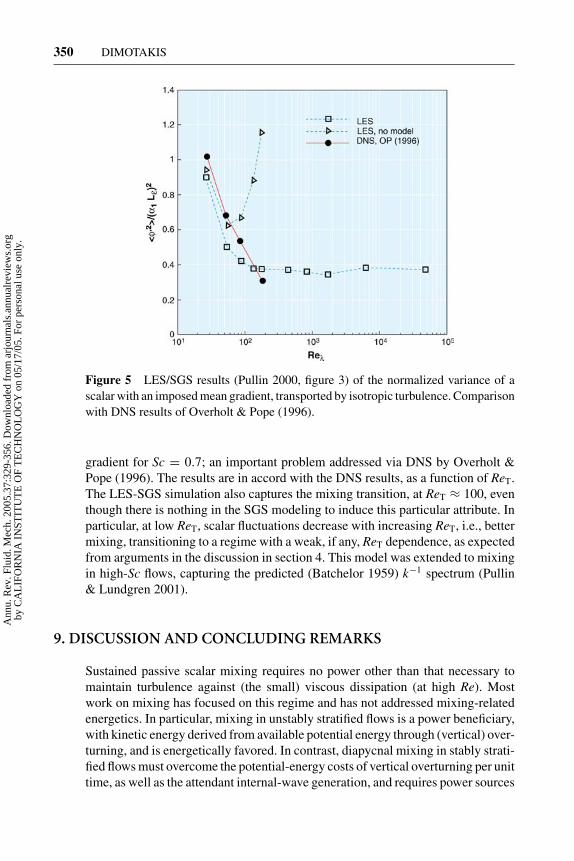
Figure 5 LES/SGS results (Pullin 2000, figure 3) of the normalized variance of ascalar with an imposed mean gradient, transported by isotropic turbulence. Comparisonwith DNS results of Overholt & Pope (1996).

gradient for Sc = 0.7; an important problem addressed via DNS by Overholt &Pope (1996). The results are in accord with the DNS results, as a function of ReT.The LES-SGS simulation also captures the mixing transition, at ReT ≈ 100, eventhough there is nothing in the SGS modeling to induce this particular attribute. Inparticular, at low ReT, scalar fluctuations decrease with increasing ReT, i.e., bettermixing, transitioning to a regime with a weak, if any, ReT dependence, as expectedfrom arguments in the discussion in section 4. This model was extended to mixingin high-Sc flows, capturing the predicted (Batchelor 1959) k−1 spectrum (Pullin& Lundgren 2001).

9. DISCUSSION AND CONCLUDING REMARKS

Sustained passive scalar mixing requires no power other than that necessary tomaintain turbulence against (the small) viscous dissipation (at high Re). Mostwork on mixing has focused on this regime and has not addressed mixing-relatedenergetics. In particular, mixing in unstably stratified flows is a power beneficiary,with kinetic energy derived from available potential energy through (vertical) over-turning, and is energetically favored. In contrast, diapycnal mixing in stably strati-fied flows must overcome the potential-energy costs of vertical overturning per unittime, as well as the attendant internal-wave generation, and requires power sources

Ann

u. R

ev. F

luid

. Mec

h. 2

005.

37:3

29-3

56. D

ownl

oade

d fr

om a

rjou

rnal

s.an

nual

revi

ews.

org

by C

AL

IFO

RN

IA I

NST

ITU

TE

OF

TE

CH

NO

LO

GY

on

05/1

7/05

. For

per

sona

l use

onl

y.



(substantially) larger than those required to overcome the (small) viscous-dissipa-tion losses. In the atmosphere, mixing would primarily occur in the planetaryboundary layer, jet stream (clear-air turbulence), and as a consequence of moist-air/cloud dynamics, were it not for important energetic events such as storms andhurricanes. A similar picture emerges in ocean mixing, which could well be dom-inated by ocean-current wakes and stirring at rough bottom and shelf topography,and internal-wave breaking. In deep ocean flows, the power budget that sustainsthis process is an important issue in ocean and global dynamics and a research topic(Wunsch & Ferrari 2004). Level-3 mixing, as in the case of combustion briefly dis-cussed here, can tap energy sources far exceeding the kinetic energy of the flow thatbrings reactants together and can alter the dynamics in qualitative and quantitativeways. Under these circumstances, coupling between mixing and flow dynamicscan be very strong, especially in confined flows, where dilatation can induce largepressure rise/gradients that are exploited for propulsion, explosions, etc.

Regarding future progress, the discussion here places the greatest hopes forunderstanding turbulence and mixing on experiments and LES-SGS modelingand computation, with much that is fruitful and important remaining to be done.Experimentally, the combination of continuously improving optical/laser diagnos-tics, digital-imaging, and data-acquisition techniques holds the promise of suffi-ciently resolved, high-quality, 3D data as a function of time, in moderate- to post-transitional-Re flows. Such experimental data can provide the means to probe thefull dimensionality of turbulence and mixing, perhaps for the first time, permittingvalidations of turbulence and SGS models that are not constrained to comparisonswith simple average profiles or low-order statistics, focusing on observations moreclosely related to mixing. Regarding theory, modeling, and simulations, one caneasily argue that ever-faster computing, although welcome, will not by itself pro-duce sufficient near-term progress. Considering LES-SGS, the discussion here alsoplaces hopes on models that respect physical SGS dynamics and correctly modelthe response to anisotropy, density inhomogeneneity, etc. Such models are neededto represent SGS dynamics in stratified and accelerated flows, and to incorpo-rate such SGS contributions as baroclinic vorticity generation, extensions to theidiosyncrasies of near-wall turbulence, dilatation, as well as realistic scalar PDFmodeling coupled with improved reduced-kinetics schemes for combustion. Suchextensions will be necessary to address Level-2 and Level-3 mixing, as well asmixing in compressible turbulent flows.

ACKNOWLEDGMENTS

Support for this review by AFOSR Grants F49620–01–1–0006 and FA9550–04–1–0020, the DOE/Caltech ASCI/ASAP subcontract B341492, and the Caltech JohnK. Northrop Chair is gratefully acknowledged. I would also like to acknowledgeboth recent and previous discussions with and assistance by J. Adkins and W.R.C.Phillips on ocean mixing; D. Arnett, H. Bethe, and R. Lovelace on astrophysicsand supernova explosions; J.E. Broadwell and M.G. Mungal on passive-scalar

Ann

u. R

ev. F

luid

. Mec

h. 2

005.

37:3

29-3

56. D

ownl

oade

d fr

om a

rjou

rnal

s.an

nual

revi

ews.

org

by C

AL

IFO

RN

IA I

NST

ITU

TE

OF

TE

CH

NO

LO

GY

on

05/1

7/05

. For

per

sona

l use

onl

y.


352 DIMOTAKIS

mixing; A.W. Cook, T.W. Mattner, D.I. Meiron, and P.L. Miller on RTI flow; H.J.S.Fernando, A. Mahalov, and J. Riley on mixing in stably stratified flows; H. Lamon scalar transport and diffusion; H.W. Liepmann on turbulence; C. Pantano onmixing and combustion dynamics; T.W. Mattner and D.I. Pullin on sub-grid scalemodeling; and R.A. Shaw on particle and cloud dynamics; as well as assistancewith the text by J.M. Bergthorson and D.I. Pullin.

The Annual Review of Fluid Mechanics is online at http://fluid.annualreviews.org

LITERATURE CITED

Adkins JF, McIntyre K, Schrag DP. 2002. Thesalinity, temperature, and δ18O of the glacialdeep ocean. Science 298:1769–73

Ashurst WT, Kerstein AR, Kerr RM, GibsonCH. 1987. Alignment of vorticity and scalargradient with strain rate in simulated Navier-Stokes turbulence. Phys. Fluids 30:2343–53

Batchelor GK. 1959. Small-scale variation ofconvected quantities like temperature in tur-bulent fluid. Part 1. General discussion andthe case of small conductivity. J. Fluid Mech.5:113–33

Batchelor GK. 1967. An Introduction to FluidDynamics. Cambridge, UK: CambridgeUniv. Press

Batt RG. 1977. Turbulent mixing of passive andchemically reacting species in a low-speedshear layer. J. Fluid Mech. 82:53–95

Bethe HA, Wilson JR. 1985. Revival of a stalledsupernova shock by neutrino heating. Astro-phys. J. 295:14–23

Bernal LP. 1988. The statistics of the organizedvortical structure in turbulent mixing layers.Phys. Fluids 31:2533–43

Bilger RW, Saetran LR, Krishnamoorthy LV.1991. Reaction in a scalar mixing layer. J.Fluid Mech. 233:211–42

Bond CL. 1999. Reynolds Number Effects onMixing in the Turbulent Shear Layer. PhDthesis. Calif. Inst. Technol.

Broadwell JE, Breidenthal RE. 1982. A sim-ple model of mixing and chemical reactionin a turbulent shear layer. J. Fluid Mech.125:397–410

Broadwell JE, Mungal MG. 1991. Large-scale

structures and molecular mixing. Phys. Flu-ids 3:1193–206

Buckmaster J. 2002. Edge-flames. Prog. Energ.Combust. Sci. 28:435–75

Burrows A. 2000. Supernova explosions in theuniverse. Nature 403:727–33

Chandrasekhar S. 1955. The character of theequilibrium of an incompressible heavy vis-cous fluid of variable density. Proc. Cam-bridge Philos. Soc. 51:162–78

Chandrasekhar S. 1961. Hydrodynamic and Hy-dromagnetic Stability. Oxford: Oxford Univ.Press. 1981. New York: Dover

Colgate SA, White RH. 1966. The hydro-dynamic behavior of supernova explosions.Astrophys. J. 143:626–81

Cook AW, Dimotakis PE. 2001. Transitionstages of Rayleigh-Taylor instability be-tween miscible fluids. J. Fluid Mech. 443:69–99

Cook AW, Dimotakis PE. 2002. Corrigen-dum—Transition stages of Rayleigh-Taylorinstability between miscible fluids. J. FluidMech. 457:410–11

Cook AW, Zhou Y. 2002. Energy transferin Rayleigh-Taylor instability. Phys. Rev. E66:026312

Corrsin S. 1961. The reactant concentrationspectrum in turbulent mixing with first-orderreaction. J. Fluid Mech. 11:407–16

Corrsin S. 1964. Further consideration of On-sager’s cascade model for turbulent spectra.Phys. Fluids 7:1156–59

Dahm WJA, Dimotakis PE. 1987. Measure-ments of entrainment and mixing in turbulentjets. AIAA J. 25:1216–23

Ann

u. R

ev. F

luid

. Mec

h. 2

005.

37:3

29-3

56. D

ownl

oade

d fr

om a

rjou

rnal

s.an

nual

revi

ews.

org

by C

AL

IFO

RN

IA I

NST

ITU

TE

OF

TE

CH

NO

LO

GY

on

05/1

7/05

. For

per

sona

l use

onl

y.



Danaila L, Anselmet F, Antonia RA. 2002. Anoverview of the effect of large-scale inho-mogeneities on small-scale turbulence. Phys.Fluids 14:2475–84

Danaila L, Mydlarski L. 2001. Effect ofgradient production on scalar fluctuationsin decaying grid turbulence. Phys. Rev. E64:016316

Davies RM, Taylor GI. 1950. The mechanicsof large bubbles rising through extended liq-uids and through liquids in tubes. Proc. R.Soc. London Ser. A 200:375–90

de Bruyn Kops SM, Riley JJ, Kosaly G.2001. Direct numerical simulation of re-acting scalar mixing layers. Phys. Fluids13:1450–65

Dimonte G, Schneider M. 2000. Density ratiodependence of Rayleigh-Taylor mixing forsustained and impulsive acceleration histo-ries. Phys. Fluids 12:304–21

Dimotakis PE. 1986. Two-dimensional shear-layer entrainment. AIAA J. 24:1791–96

Dimotakis PE. 1989. Turbulent shear layer mix-ing with fast chemical reactions. In TurbulentReactive Flows. Lect. Notes Eng. 40:417–85.New York: Springer-Verlag

Dimotakis PE. 1991. Turbulent free shear layermixing and combustion. In High SpeedFlight Propulsion Systems. Prog. Astronaut.Aeronaut. 137:265–340

Dimotakis PE. 2000. The mixing transition inturbulent flow. J. Fluid Mech. 409:69–98

Dimotakis PE. 2001. Recent advances in turbu-lent mixing. In Mechanics for a New Millen-nium, ed. H Aref, JW Phillips, pp. 327–44.Dordrecht: Kluwer

Dimotakis PE, Catrakis HJ. 1999. Turbulence,fractals, and mixing. In Mixing: Chaos andTurbulence, ed. H Chate, E Willermaux, JMChomaz, pp. 59–143. New York: Kluwer

Dimotakis PE, Miake-Lye RC, PapantoniouDA. 1983. Structure and dynamics ofround turbulent jets. Phys. Fluids 26:3185–92

Dold JW. 1988. Flame propagation in a nonuni-form mixture: the structure of anchored tripleflames. Prog. Astro. Aero. 113:240–48

Dowling DR, Dimotakis PE. 1990. Similarity

of the concentration field of gas-phase turbu-lent jets. J. Fluid Mech. 218:109–41

Eckart C. 1948. An analysis of the stirring andmixing processes in incompressible fluids. J.Mar. Res. 7:265–75

Falkovich G, Fouxon A, Stepanov MG. 2002.Acceleration of rain initiation by cloud tur-bulence. Nature 419:151–54

Fermi E, von Neumann J. 1955. Taylor insta-bility of incompressible liquids. Los AlamosSci. Lab. Rep. AECU–2979

Frieler CE. 1992. Mixing and reaction in thesubsonic 2-D turbulent shear layer. PhD the-sis. Calif. Inst. Technol.

George WK. 1989. The self-preservation of tur-bulent flows and its relation to initial condi-tions and coherent structures. In Advancesin Turbulence, ed. WK George, R Arndt, pp.39–74. New York: Hemisphere

Germano M. 1992. Turbulence, the filtering ap-proach. J. Fluid Mech. 238:325–36

Germano M, Piomelli U, Moin P, Cabot W.1991. A dynamic subgrid-scale eddy viscos-ity model. Phys. Fluids 3:1760–65

Glezer A. 1988. The formation of vortex rings.Phys. Fluids 31:3532–42

Hermanson JC, Dimotakis PE. 1989. Effectsof heat release in a turbulent, reacting shearlayer. J. Fluid Mech. 199:333–75

Hill JC. 1976. Homogeneous turbulent mix-ing with chemical reaction. Annu. Rev. FluidMech. 8:135–61

Hirschfelder JO, Curtiss CF, Bird RB. 1954.Molecular Theory of Gases and Liquids.New York: Wiley

Howard LN. 1962. Note on a paper of John W.Miles. J. Fluid Mech. 10:509–12

Janka H-Th. 2002. The secrets behind super-novae. Science 297:1183–84

Jimenez J, Wray AA. 1998. On the character-istics of vortex filaments in isotropic turbu-lence. J. Fluid Mech. 373:255–85

Jimenez J, Wray AA, Saffman PG, Rogallo RS.1993. The structure of intense vorticity inhomogeneous isotropic turbulence. J. FluidMech. 255:65–90

Kennedy IM, Kent JH. 1978. Measurementsof a conserved scalar in turbulent jet

Ann

u. R

ev. F

luid

. Mec

h. 2

005.

37:3

29-3

56. D

ownl

oade

d fr

om a

rjou

rnal

s.an

nual

revi

ews.

org

by C

AL

IFO

RN

IA I

NST

ITU

TE

OF

TE

CH

NO

LO

GY

on

05/1

7/05

. For

per

sona

l use

onl

y.


354 DIMOTAKIS

diffusion flames. Proc. Combust. Inst. 17:279–87

Kolmogorov AN. 1941. Local structure of tur-bulence in an incompressible viscous fluidat very high reynolds numbers. Dokl. Akad.Nauk SSSR 30:301–5

Kolmogorov AN. 1962. A refinement of pre-vious hypotheses concerning the local struc-ture of turbulence in a viscous incompress-ible fluid at high Reynolds number. J. FluidMech. 13:82–85

Koochesfahani MM, Dimotakis PE. 1986. Mix-ing and chemical reactions in a turbulentliquid mixing layer. J. Fluid Mech. 170:83–112

Kosaly G. 1993. Frequency spectra of reactantfluctuations in turbulent flows. J. Fluid Mech.246:489–502

Landau LD, Lifshitz EM. 1997. Course ofTheoretical Physics, Vol. 6. Fluid Mechan-ics London: Pergammon. 2nd ed.

Langmuir I. 1938. Surface motion of water in-duced by wind. Science 87:119–23

Lapeyre G, Held IM. 2003. Diffusivity, kineticenergy dissipation, and closure theories forthe poleward eddy heat flux. J. Atmos. Sci.60:2907–16

Leonard A. 1974. Energy cascade in large-eddy simulations of turbulent fluid flows.Adv. Geophys. 18:237–49

Leonard A. 1997. Large-eddy simulation ofchaotic convection and beyond. AIAA Paper97–0204

Lesieur M, Metais O. 1996. New trends in large-eddy simulations of turbulence. Annu. Rev.Fluid Mech. 28:45–82

Lundgren TS. 1982. Strained spiral vortexmodel for turbulent fine structure. Phys. Flu-ids 25:2193–203

Lundgren TS. 1985. The concentration spec-trum of the product of a fast bimolecularreaction. Chem. Eng. Sci. 40:1641–52

Lundgren TS. 2002. Kolmogorov two-thirdslaw by matched asymptotic expansion. Phys.Fluids 14:638–42

Lundgren TS. 2003. Kolmogorov turbulence bymatched asymptotic expansions. Phys. Flu-ids 15:1074–81

Meneveau C, Lund T, Cabot W. 1996. A La-grangian dynamic subgrid-scale model ofturbulence. J. Fluid Mech. 319:353–85

Meneveau C, O’Neil J. 1994. Scaling laws ofthe dissipation rate of turbulent subgrid-scalekinetic energy. Phys. Rev. E 49:2866–74

Meshkov EE. 1969. Instability of the interfaceof two gases accelerated by a shock wave.Sov. Fluid Dyn. 4:101–4

Miles JW. 1961. On the stability of heteroge-neous shear flows. J. Fluid Mech. 10:496–508

Miller MF, Bowman CT, Mungal MG. 1998. Anexperimental investigation of the effects ofcompressibility on a turbulent reacting mix-ing layer. J. Fluid Mech. 356:25–64

Miller PL, Dimotakis PE. 1996. Measurementsof scalar power spectra in high Schmidt num-ber turbulent jets. J. Fluid Mech. 308:129–46

Misra A, Pullin DI. 1997. A vortex-based sub-grid stress model for large-eddy simulation.Phys. Fluids 9:2443–54

Moin P, Squires K, Cabot W, Lee S. 1991. A dy-namic subgrid-scale model for compressibleturbulence and scalar transport. Phys. Fluids3:2746–57

Monin AS, Yaglom AM. 1975. Statistical FluidMechanics: Mechanics of Turbulence, ed. JLumley, Vol. II. Cambridge, MA: MIT Press

Moser RD, Zandonade P. 2003. Developmentof high Reynolds number optimal LES mod-els. In Reynolds Number Scaling in TurbulentFlow, ed. AJ Smits, pp. 169–74. Dordrecht:Kluwer

Mungal MG, Dimotakis PE. 1984. Mixing andcombustion with low heat release in a turbu-lent mixing layer. J. Fluid Mech. 148:349–82

Mungal MG, Hermanson JC, Dimotakis PE.1985. Reynolds number effects on mixingand combustion in a reacting shear layer.AIAA J. 23:1418–23

Oboukhov AM. 1962. Some specific featuresof atmospheric turbulence. J. Fluid Mech.13:77–81

O’Brien EE. 1968. Lagrangian history directinteraction equations for isotropic turbulentmixing under a second-order chemical reac-tion. Phys. Fluids 11:2328–35

Ann

u. R

ev. F

luid

. Mec

h. 2

005.

37:3

29-3

56. D

ownl

oade

d fr

om a

rjou

rnal

s.an

nual

revi

ews.

org

by C

AL

IFO

RN

IA I

NST

ITU

TE

OF

TE

CH

NO

LO

GY

on

05/1

7/05

. For

per

sona

l use

onl

y.



Overholt MR, Pope SB. 1996. Direct numericalsimulation of a passive scalar with imposedmean gradient in isotropic turbulence. Phys.Fluids 8:3128–48

Pantano C. 2004. Direct simulation of non-premixed flame extinction in a methane-airjet with reduced chemistry. J. Fluid Mech.514:231–70

Pantano C, Sarkar S, Williams FA. 2003. Mix-ing of a conserved scalar in a turbulentreacting shear layer. J. Fluid Mech. 481:291–328

Pao YH. 1964. Statistical behavior of a turbu-lent multicomponent mixture with first-orderreactions. AIAA J. 2:1550–59

Papavassiliou DV. 2002. Turbulent transportfrom continuous sources at the wall of a chan-nel. Int. J. Heat Mass Transf. 45:3571–83

Papavassiliou DV, Hanratty TJ. 1997. Transportof a passive scalar in a turbulent channel flow.Int. J. Heat Mass Transf. 40:1301–11

Pasquero C, Provenzale A, Babiano A. 2001.Parameterization of dispersion in two-dimensional turbulence. J. Fluid Mech. 439:279–303

Peltier WR, Caulfield CP. 2003. Mixing effi-ciency in stratified shear flows. Annu. Rev.Fluid Mech. 35:135–67

Peters N. 1985. Numerical and asymptoticanalysis of systematically reduced reactionschemes for hydrocarbon flames. Lect. NotesPhys. 241:90–109

Peters N. 2000. Turbulent Combustion. Cam-bridge, UK: Cambridge Univ. Press

Phillips WRC. 2001a. On the pseudomomen-tum and generalized Stokes drift in a spec-trum of rotational waves. J. Fluid Mech.430:209–29

Phillips WRC. 2001b. On an instability to Lang-muir circulations and the role of Prandtland Richardson numbers. J. Fluid Mech.442:335–58

Phillips WRC. 2002. Langmuir circulations be-neath growing or decaying surface waves. J.Fluid Mech. 469:317–42

Phillips WRC. 2004. On the spacing of Lang-muir circulation in strong shear. J. FluidMech. Accepted

Pope S. 2000. Turbulent Flows. Cambridge,UK: Cambridge Univ. Press

Porte-Agel F, Meneveau C, Parlange MB. 2000.A scale-dependent dynamic model for large-eddy simulation: application to a neutral at-mospheric boundary layer. J. Fluid Mech.415:261–84

Pullin DI. 2000. A vortex-based model for thesubgrid flux of a passive scalar. Phys. Fluids12:2311–19

Pullin DI, Lundgren TS. 2001. Axial motionand scalar transport in stretched spiral vor-tices. Phys. Fluids 13:2553–63

Pullin DI, Saffman PG. 1994. Reynolds stressesand one-dimensional spectra for a vortexmodel of homogeneous anisotropic turbu-lence. Phys. Fluids 6:1787–96

Rayleigh. 1883. Investigation of the character ofthe equilibrium of an incompressible heavyfluid of variable density. Proc. London Math.Soc. 14:170–77

Richtmyer RD. 1960. Taylor instability in shockacceleration of compressible fluids. Com-mun. Pure Appl. Math. 13:297–319

Riley JJ, Lelong M-P. 2000. Fluid motions inthe presence of strong stable stratification.Annu. Rev. Fluid Mech. 32:613–57

Robinson A. 1956. On the motion of small par-ticles in a potential field of flow. Commun.Pure Appl. Math. 9:69–84

Saffman PG. 1960. On the effect of the molecu-lar diffusivity in turbulent diffusion. J. FluidMech. 8:273–83

Sawford B. 2001. Turbulent relative dispersion.Annu. Rev. Fluid Mech. 33:289–317

Schneider T. 2004. The tropopause and thethermal stratification in the extratropics ofa dry atmosphere. J. Atmos. Sci. 61:1317–40

Scotti A, Meneveau C. 1999. A fractal modelfor large-eddy simulation of turbulent flow.Phys. D 127:198–232

Shan JW, Dimotakis PE. 2001. Turbulentmixing in liquid-phase transverse jets. http://resolver.library.caltech.edu/CaltechGalcitFM:2001.006

Sharp DH. 1984. An overview of Rayleigh-Taylor instability. Phys. D 12:3–18

Ann

u. R

ev. F

luid

. Mec

h. 2

005.

37:3

29-3

56. D

ownl

oade

d fr

om a

rjou

rnal

s.an

nual

revi

ews.

org

by C

AL

IFO

RN

IA I

NST

ITU

TE

OF

TE

CH

NO

LO

GY

on

05/1

7/05

. For

per

sona

l use

onl

y.


356 DIMOTAKIS

Shaw RA. 2003. Particle-turbulence interac-tions in atmospheric clouds. Annu. Rev. FluidMech. 35:183–227

Shaw RA, Reade WC, Collins LR, VerlindeJ. 1998. Preferential concentration of clouddroplets by turbulence: effects on the earlyevolution of cumulus cloud droplet spectra.J. Atmos. Sci. 55:1965–76

Slessor MD. 1998. Aspects of turbulent-shear-layer dynamics and mixing. PhD thesis.Calif. Inst. Technol.

Slessor MD, Bond CL, Dimotakis PE.1998. Turbulent shear-layer mixing at highReynolds numbers: effects of inflow condi-tions. J. Fluid Mech. 376:115–38

Smith JA. 1992. Observed growth of Lang-muir circulation. J. Geophys. Res. 97:5651–64

Smith JA. 1998. Evolution of Langmuir circula-tion in a storm. J. Geophys. Res. 103:12649–68

Smith KS, Boccaletti G, Henning CC, MarinovI, Tam CY, et al. 2002. Turbulent diffusionin the geostrophic inverse cascade. J. FluidMech. 469:13–48

Sreenivasan KR. 1991. Fractals and multifrac-tals in fluid turbulence. Annu. Rev. FluidMech. 23:539–600

Taylor GI. 1935. Statistical theory of turbu-lence: Parts I–II. Proc. Roy. Soc. London A151:421–64

Taylor GI. 1950. The instability of liquid sur-faces when accelerated in a direction perpen-dicular to their planes. Proc. R. Soc. LondonSer. A 201:192–96

Taylor GI. 1953. Dispersion of soluble matter insolvent flowing slowly through a tube. Proc.R. Soc. London Ser. A 219:186–203

Taylor GI. 1954. The dispersion of matter inturbulent flow through a pipe. Proc. R. Soc.London Ser. A 223:446–68

Tennekes H, Lumley JL. 1972. A First Coursein Turbulence. Cambridge, MA: MIT Press

Thorpe SA. 2004. Langmuir circulation. Annu.Rev. Fluid Mech. 36:55–79

Toor HL. 1962. Mass transfer in dilute turbu-lent and nonturbulent systems with rapid ir-reversible reactions and equal diffusivities.AIChE J. 8:70–78

Turner JS. 1973. Buoyancy Effects in Fluids.Cambridge, UK: Cambridge Univ. Press

Tziperman E. 1986. On the role of interiormixing and air-sea fluxes in determining thestratification and circulation of the oceans.J. Phys. Oceanogr. 16:680–93

Van Atta C, Antonia R. 1980. Reynolds numberdependence of skewness and flatness factorsof velocity gradients. Phys. Fluids 23:252–57

Veron F, Melville WK. 2001. Experiments onthe stability and transition of wind-drivenwater surfaces. J. Fluid Mech. 446:25–65

Vervisch L, Poinsot T. 1998. Direct numericalsimulation of non-premixed turbulent flames.Annu. Rev. Fluid Mech. 30:655–91

Villermaux E. 2002. Mixing as an aggrega-tion process. IUTAM Symp. Turbulent Mix-ing Combustion. 3–6 June 2001, pp. 1–21,Kingston, Ontario, Can.

Voelkl T, Pullin DI, Chan DC. 2000. Aphysical-space version of the stretched-vortex subgrid-stress model for large-eddysimulation. Phys. Fluids 12:1810–25

Wallace AK. 1981. Experimental investigationof the effects of chemical heat release in thereacting turbulent plane shear layer. PhDthesis. Univ. Adelaide

Warhaft Z. 2000. Passive scalars in turbulentflows. Annu. Rev. Fluid Mech. 32:203–40

Williams FA. 1985. Combustion Theory. MenloPark, CA: Benjamin/Cummings

Wunsch C. 2002. What is the thermohaline cir-culation? Science 298:1179–81

Wunsch C, Ferrari R. 2004. Vertical mixing,energy, and the general circulation of theoceans. Annu. Rev. Fluid Mech. 36:281–314

Ann

u. R

ev. F

luid

. Mec

h. 2

005.

37:3

29-3

56. D

ownl

oade

d fr

om a

rjou

rnal

s.an

nual

revi

ews.

org

by C

AL

IFO

RN

IA I

NST

ITU

TE

OF

TE

CH

NO

LO

GY

on

05/1

7/05

. For

per

sona

l use

onl

y.

P1: JRX

November 24, 2004 12:5 Annual Reviews AR235-FM

Annual Review of Fluid MechanicsVolume 37, 2005

CONTENTS

ROBERT T. JONES, ONE OF A KIND, Walter G. Vincenti 1

GEORGE GABRIEL STOKES ON WATER WAVE THEORY,Alex D.D. Craik 23

MICROCIRCULATION AND HEMORHEOLOGY, Aleksander S. Popeland Paul C. Johnson 43

BLADEROW INTERACTIONS, TRANSITION, AND HIGH-LIFT AEROFOILSIN LOW-PRESSURE TURBINES, Howard P. Hodsonand Robert J. Howell 71

THE PHYSICS OF TROPICAL CYCLONE MOTION, Johnny C.L. Chan 99

FLUID MECHANICS AND RHEOLOGY OF DENSE SUSPENSIONS, JonathanJ. Stickel and Robert L. Powell 129

FEEDBACK CONTROL OF COMBUSTION OSCILLATIONS, Ann P. Dowlingand Aimee S. Morgans 151

DISSECTING INSECT FLIGHT, Z. Jane Wang 183

MODELING FLUID FLOW IN OIL RESERVOIRS, Margot G. Gerritsenand Louis J. Durlofsky 211

IMMERSED BOUNDARY METHODS, Rajat Mittaland Gianluca Iaccarino 239

STRATOSPHERIC DYNAMICS, Peter Haynes 263

THE DYNAMICAL SYSTEMS APPROACH TO LAGRANGIAN TRANSPORTIN OCEANIC FLOWS, Stephen Wiggins 295

TURBULENT MIXING, Paul E. Dimotakis 329

GLOBAL INSTABILITIES IN SPATIALLY DEVELOPING FLOWS:NON-NORMALITY AND NONLINEARITY, Jean-Marc Chomaz 357

GRAVITY-DRIVEN BUBBLY FLOWS, Robert F. Mudde 393

PRINCIPLES OF MICROFLUIDIC ACTUATION BY MODULATION OFSURFACE STRESSES, Anton A. Darhuber and Sandra M. Troian 425

MULTISCALE FLOW SIMULATIONS USING PARTICLES,Petros Koumoutsakos 457

vii

Ann

u. R

ev. F

luid

. Mec

h. 2

005.

37:3

29-3

56. D

ownl

oade

d fr

om a

rjou

rnal

s.an

nual

revi

ews.

org

by C

AL

IFO

RN

IA I

NST

ITU

TE

OF

TE

CH

NO

LO

GY

on

05/1

7/05

. For

per

sona

l use

onl

y.

turbulent mixing

Documents