Turing Oracle Machines, Online Computing, and

Three Displacements in Computability Theory

Robert I. Soare∗

January 3, 2009

Contents

1 Introduction 41.1 Terminology: Incompleteness and Incomputability . . . . . . 41.2 The Goal of Incomputability not Computability . . . . . . . 51.3 Computing Relative to an Oracle or Database . . . . . . . . . 51.4 Continuous Functions and Calculus . . . . . . . . . . . . . . . 6

2 Origins of Computability and Incomputability 72.1 Godel’s Incompleteness Theorem . . . . . . . . . . . . . . . . 72.2 Alonzo Church . . . . . . . . . . . . . . . . . . . . . . . . . . 82.3 Herbrand-Godel Recursive Functions . . . . . . . . . . . . . . 92.4 Stalemate at Princeton Over Church’s Thesis . . . . . . . . . 102.5 Godel’s Thoughts on Church’s Thesis . . . . . . . . . . . . . . 11

3 Turing Breaks the Stalemate 113.1 Turing Machines and Turing’s Thesis . . . . . . . . . . . . . . 113.2 Godel’s Opinion of Turing’s Work . . . . . . . . . . . . . . . . 13

3.2.1 Godel [193?] Notes in Nachlass [1935] . . . . . . . . . 143.2.2 Princeton Bicentennial [1946] . . . . . . . . . . . . . . 15

∗Parts of this paper were delivered in an address to the conference, Computation andLogic in the Real World, at Siena, Italy, June 18–23, 2007. Keywords: Turing ma-chine, automatic machine, a-machine, Turing oracle machine, o-machine, Alonzo Church,Stephen C. Kleene, Alan Turing, Kurt Godel, Emil Post, computability, incomputability,undecidability, Church-Turing Thesis, Post-Turing Thesis on relative computability, com-putable approximations, Limit Lemma, effectively continuous functions, computability inanalysis, strong reducibilities. Thanks are due to C.G. Jockusch, Jr., P. Cholak, andT. Slaman for corrections and suggestions.

1

3.2.3 The Flaw in Church’s Thesis . . . . . . . . . . . . . . 163.2.4 Godel on Church’s Thesis . . . . . . . . . . . . . . . . 173.2.5 Godel’s Letter to Kreisel [1968] . . . . . . . . . . . . . 173.2.6 Gibbs Lecture [1951] . . . . . . . . . . . . . . . . . . . 173.2.7 Godel’s Postscriptum 3 June, 1964 to Godel [1934] . . 18

3.3 Hao Wang Reports on Godel . . . . . . . . . . . . . . . . . . 193.4 Kleene’s Remarks About Turing . . . . . . . . . . . . . . . . 193.5 Church’s Remarks About Turing . . . . . . . . . . . . . . . . 20

4 Oracle Machines and Relative Computability 204.1 Turing’s Oracle Machines . . . . . . . . . . . . . . . . . . . . 214.2 Modern Definitions of Oracle Machines . . . . . . . . . . . . . 21

4.2.1 The Graph of a Partial Computable Function . . . . . 234.2.2 The Graph of an Oracle Computable Functional . . . 23

4.3 The Oracle Graph Theorem . . . . . . . . . . . . . . . . . . . 234.4 Equivalent Definitions of Relative Computability . . . . . . . 24

4.4.1 Notation for Functions and Functionals . . . . . . . . 25

5 Emil Post Expands Turing’s Ideas 255.1 Post’s Work in the 1930’s . . . . . . . . . . . . . . . . . . . . 265.2 Post Steps Into Turing’s Place During 1940–1954 . . . . . . . 265.3 Post’s Problem on Incomplete C.E. Sets . . . . . . . . . . . . 285.4 Post Began With Strong Reducibilities . . . . . . . . . . . . . 28

6 Post Highlights Turing Computability 296.1 Post Articulates Turing Reducibility . . . . . . . . . . . . . . 296.2 The Post-Turing Thesis . . . . . . . . . . . . . . . . . . . . . 30

7 Continuous and Total Functionals 317.1 Representations of Open and Closed Sets . . . . . . . . . . . 317.2 Notation for Trees . . . . . . . . . . . . . . . . . . . . . . . . 317.3 Dense Open Subsets of Cantor Space . . . . . . . . . . . . . . 337.4 Effectively Open and Closed Sets . . . . . . . . . . . . . . . . 337.5 Continuous Functions on Cantor Space . . . . . . . . . . . . . 347.6 Effectively Continuous Functionals . . . . . . . . . . . . . . . 357.7 Continuous Functions are Relatively Computable . . . . . . . 36

8 Bounded Reducibilities 368.1 A Matrix Mx for Bounded Reducibilities . . . . . . . . . . . . 368.2 Bounded Turing Reducibility . . . . . . . . . . . . . . . . . . 37

2

8.3 Truth-Table Reductions . . . . . . . . . . . . . . . . . . . . . 378.4 Difference of c.e. sets, n-c.e., and ω-c.e. sets . . . . . . . . . . 39

9 Online Computing 409.1 Turing Machines and Online Processes . . . . . . . . . . . . . 429.2 Trial and Error Computing . . . . . . . . . . . . . . . . . . . 429.3 The Limit Lemma . . . . . . . . . . . . . . . . . . . . . . . . 439.4 Two Models for Computing With Error . . . . . . . . . . . . 44

9.4.1 The Limit Computable Model . . . . . . . . . . . . . . 449.4.2 The Online Model . . . . . . . . . . . . . . . . . . . . 44

10 Three Displacements in Computability Theory 45

11 “Computable” versus “Recursive” 4511.1 Church Defends Church’s Thesis with “Recursive” . . . . . . 4611.2 Church and Kleene Define “Recursive” as “Computable” . . . 4611.3 Godel Rejects “Recursive Function Theory” . . . . . . . . . . 4711.4 The Ambiguity in the Term “Recursive” . . . . . . . . . . . . 4811.5 Changing “Recursive” Back to “Inductive” . . . . . . . . . . 48

12 Renaming it the “Computability Thesis?” 5012.1 Kleene Called it “Thesis I” in [1943] . . . . . . . . . . . . . . 5012.2 Kleene Named it “Church’s thesis” in [1952] . . . . . . . . . . 5012.3 Kleene Dropped “Thesis I” for “Church’s thesis” . . . . . . . 5112.4 Evidence for the Computability Thesis . . . . . . . . . . . . . 5112.5 Who First Demonstrated the Computability Thesis? . . . . . 5212.6 The Computability Thesis and the Calculus . . . . . . . . . . 5412.7 Founders of Computability and the Calculus . . . . . . . . . . 55

13 Turing a-machines versus o-machines? 5713.1 Turing, Post, and Kleene on Relative Computability . . . . . 5713.2 Relative Computability Unifies Incomputability . . . . . . . . 5713.3 The Key Concept of the Subject . . . . . . . . . . . . . . . . 5713.4 When to Introduce Relative Computability . . . . . . . . . . 58

14 Conclusions 59

Abstract

We begin with the history of the discovery of computability in the1930’s, the roles of Godel, Church, and Turing, and the formalisms ofrecursive functions and Turing automatic machines (a-machines). To

3

whom did Godel credit the definition of a computable function? Wepresent Turing’s notion [1939, §4] of an oracle machine (o-machine)and Post’s development of it in [1944, §11], [1948], and finally Kleene-Post [1954] into its present form.

A number of topics arose from Turing functionals including con-tinuous functionals on Cantor space and online computations. Almostall the results in theoretical computability use relative reducibility ando-machines rather than a-machines and most computing processes inthe real world are potentially online or interactive. Therefore, we arguethat Turing o-machines, relative computability, and online computingare the most important concepts in the subject, more so than Turinga-machines and standard computable functions since they are specialcases of the former and are presented first only for pedagogical clar-ity to beginning students. At the end in §10 – §13 we consider threedisplacements in computability theory, and the historical reasons theyoccurred. Several brief conclusions are drawn in §14.

1 Introduction

In this paper we consider the development of Turing oracle machines andrelative computability and its relation to continuity in analysis and to onlinecomputing in the real world. We also challenge a number of traditional viewsof these subjects as often presented in the literature since the 1930’s.

1.1 Terminology: Incompleteness and Incomputability

The two principal accomplishments in computability and logic in the 1930’swere the discovery of incompleteness by Godel [1931] and of incomputabil-ity independently by Church [1936] and Turing in [1936]. We use the term“noncomputable” or “incomputable” for individual instances, but we of-ten use the term “incomputability” for the general concept because it islinguistically and mathematically parallel to “incomplete.” The term “in-computable” appeared in English as early as 1606 with the meaning, thatwhich “cannot be computed or reckoned; incalculable,” according to theOxford English Dictionary. Websters dictionary defines it as “greater thancan be computed or enumerated; very great.” Neither dictionary lists anentry for “noncomputable” although it has often been used in the subject tomean “not computable” for a specific function or set analogously as “non-measurable” is used in analysis.

4

1.2 The Goal of Incomputability not Computability

For several thousand years the study of algorithms had led to new the-oretical algorithms and sometimes new devices for computability and cal-culation. In the 1930’s for the first time the goal was the refutation ofHilbert’ two programs, a finite consistency proof for Peano arithmetic, andthe Entscheidungsproblem (decision problem). For the latter, two main dis-coverers of computability, Alonzo Church and Alan Turing, wanted to giveformal definitions of a computable function so that they could diagonalizeover all computable functions and produce an incomputable (unsolvable)problem. The specific models of computable functions produced by 1936,Turing a-machines, λ-definable functions, and recursive functions, wouldall have deep applications to the design and programming of computingmachines, but not until after 1940. Meanwhile, the researchers spent the re-mainder of the 1930’s investigating more of the new world of incomputabilitythey had created by diagonal arguments, just as Georg Cantor had spent thelast quarter of the nineteenth century exploring the world of uncountablesets which he had created by the diagonal method. In §1 and §2 we considerthis historical development from 1931 to 1939 and we introduce quotes fromGodel to show convincingly that he believed “the correct definition of me-chanical computability was established beyond any doubt by Turing” andonly by Turing.

1.3 Computing Relative to an Oracle or Database

In 1936 Turing’s a-machines and Church’s use of Godel’s recursive functionssolved an immediate problem by producing a definition of a computablefunction, with which one could diagonalize and produce undecidable prob-lems in mathematics. The Turing a-machine is a good model for offlinecomputing such as a calculator or batch processor where the process is ini-tially given a procedure and an input and continues with no further outsideinformation.

However, many modern computer processes are online processes in thatthey consult an external data base of other resource during the computationprocess. For example, a laptop computer might consult the World Wide Webvia an ethernet or wireless connection while it is computing. These processesare sometimes called online or interactive or database processes dependingon the way they are set up.

Turing spent 1936–1938 at Princeton writing a Ph.D. thesis under Churchon ordinal logics. A tiny and obscure part of his paper [1939, §4] included

5

a description of an oracle machine (o-machine) roughly a Turing a-machinewhich could interrogate an “oracle” (external database) during the computa-tion. The one page description was very sketchy and Turing never developedit further.

Emil Post [1944, §11] considerably expanded and developed relative com-putability and Turing functionals. These concepts were not well understoodwhen Post began, but in Post [1943], [1944], [1948] and Kleene-Post [1954]they emerged into their modern state. These are summarized in the Post-Turing Thesis of §6.2. This remarkable role by Post has been underempha-sized in the literature but is discussed here in §5 and §6.

The theory of relative computability developed by Turing and Post andthe o-machines provide a precise mathematical framework for database oronline computing just Turing a-machines provide one for offline computingprocesses such as batch processing. Oracle computing processes are thosemost often used in theoretical research and also in real world computingwhere a laptop computer may communicate with a database like the WorldWide Web. Often the local computer is called the “client” and the remotedevice the “server.”

In §4–§6 we study Turing’s oracle machines (o-machines) and Post’s de-velopment of them into relative computability. It is surprising that so muchattention has been paid to the Church-Turing Thesis 3.2 over the last sev-enty years and so little to the Post-Turing Thesis 6.1 on relative reducibil-ity, particularly in view of the importance of relative computability (Turingo-machines) in comparison with plain computability (Turing a-machines) inboth theoretical and practical areas.

1.4 Continuous Functions and Calculus

In §7 we show that any Turing functional on Cantor space 2ω is an effec-tively continuous partial map. Conversely, for any continuous functionalthere is a Turing functional relative to some real parameter which defines it,thereby linking computability with analysis. This makes Turing functionalsthe analogue in computability of the continuous functions in analysis as weexplain. In contrast, Turing a-machines viewed as functionals on Cantorspace produce only a constant functional. Surprisingly, there appears tobe more emphasis in calculus books on continuous functionals than there isin introductory computability books on computably continuous functionalsand relative computability.

6

2 Origins of Computability and Incomputability

Mathematicians have studied algorithms and computation since ancienttimes, but the modern study of computability and incomputability be-gan around 1900. David Hilbert was deeply interested in the foundationsof mathematics. Hilbert [1899] gave an axiomatization of geometry andshowed [1900] that the question of the consistency of geometry reducedto that for the real-number system, and that in turn, to arithmetic byresults of Dedekind (at least in a second order system). Hilbert [1904]proposed proving the consistency of arithmetic by what emerged [1928]as his finitist program. He proposed using the finiteness of mathematicalproofs in order to establish that contradictions could not be derived. Thistended to reduce proofs to manipulation of finite strings of symbols de-void of intuitive meaning which stimulated the development of mechanicalprocesses to accomplish this. Hilbert’s second major program concernedthe Entscheidungsproblem (decision problem). Kleene [1987b, p. 46] wrote,“The Entscheidungsproblem for various formal systems had been posed bySchroder [1895], Lowenheim [1915], and Hilbert [1918].” The decision prob-lem for first order logic emerged in the early 1920’s in lectures by Hilbert andwas stated in Hilbert and Ackermann [1928]. It was to give a decision proce-dure (Entscheidungsverfahren) “that allows one to decide the validity of thesentence.” Hilbert characterized this as the fundamental problem of mathe-matical logic. Davis [1965, p. 108] wrote, “This was because it seemed clearto Hilbert that with the solution of this problem, the Entscheidungsproblem,it should be possible, at least in principle, to settle all mathematical ques-tions in a purely mechanical manner.” Von Neumann (1927) doubted thatsuch a procedure existed but had no idea how to prove it.

2.1 Godel’s Incompleteness Theorem

Hilbert retired in 1930 and was asked to give a special address in the fall of1930 in Konigsberg, the city of his birth. Hilbert spoke on natural scienceand logic, the importance of mathematics in science, and the importanceof logic in mathematics. He asserted that there are no unsolvable problemsand stressed,

Wir mussen wissen. (We must know.)Wir werden wissen. (We will know.)

At a mathematical conference preceding Hilbert’s address, a quiet, obscureyoung man, Kurt Godel, only a year a beyond his Ph.D., announced a result

7

which would forever change the foundations of mathematics. He formalizedthe liar paradox, “This statement is false,” to prove roughly that for anyeffectively axiomatized, consistent extension T of number theory (Peanoarithmetic) there is a sentence σ which asserts its own unprovability in T .John von Neumann in the audience immediately understood the importanceof Godel’s Incompleteness Theorem. He was at the conference representingHilbert’s proof theory program, and recognized that Hilbert’s program wasover. In the next few weeks von Neuman realized that by arithmetizingthe proof of Godel’s first theorem, one could prove an even better one, thatno such formal system T could prove its own consistency. A few weekslater he brought his proof to Godel who thanked him and informed himpolitely that he had already submitted the Second Incompleteness Theoremfor publication. Godel’s Incompleteness Theorem [1931] not only refutedHilbert’s program on proving consistency, but it also had a profound ef-fect on refuting Hilbert’s second theme of the Entscheidungsproblem. Godelhad successfully challenged the Hilbert’s first proposal. This made it eas-ier to challenge Hilbert on the second topic of the decision problem. Bothrefutations used diagonal arguments. Of course, diagonal arguments hadbeen known since Cantor’s work, but Godel showed how to arithmetize thesyntactic elements of a formal system and diagonalize within that system.Crucial elements in computability theory, such as the Turing universal ma-chine, the Kleene µ-recursive functions, or the self reference in the Kleene’sRecursion Theorem, all depend upon giving code numbers to computationsand elements within a computation, and in calling algorithms by their codenumbers (Godel numbers). These ideas spring from Godel’s [1931] incom-pleteness proof.

2.2 Alonzo Church

By 1931 computability was a young man’s game. Hilbert had retired and nolonger had much influence on the field. As the importance of Godel’s Incom-pleteness Theorem began to sink in, and researchers began concentrating onthe Entscheidungsproblem, the major figures were all young. Alonzo Church(born 1903), Kurt Godel (b. 1906), and Stephen C. Kleene (b. 1909) wereall under thirty. Turing (b. 1912), perhaps the most influential of all oncomputability theory, was not even twenty. Only Emil Post (b. 1897) wasover thirty, and he was not yet thirty-five. These young men were aboutto leave Hilbert’s ideas behind and open the path of computability for thenext two thirds of the twentieth century, which would solve the theoreticalproblems and would show the way toward practical computing devices.

8

After completing his Ph.D. at Princeton in 1927, Alonzo Church spentone year at Harvard and one year at Gottingen and Amsterdam. He returnedto Princeton as an Assistant Professor of Mathematics in 1929. In 1931Church’s first student, Stephen C. Kleene, arrived at Princeton. Churchhad begun to develop a formal system now called the λ-calculus. In 1931Church knew only that the successor function was λ-definable. Kleene beganproving that certain well-known functions were λ-definable. By the timeKleene received his Ph.D. in 1934 he had shown that all the usual numbertheoretic functions were λ-definable. On the basis of this evidence andhis own intuition, Church proposed to Godel around March, 1934 the firstversion of his thesis on functions which are effectively calculable, the termin the 1930’s for a function which is computable in the informal sense. (SeeDavis [1965, p. 8–9].)

Definition 2.1. Church’s Thesis (First Version) [1934]. A functionif effectively calculable if and only if it is λ-definable.

When Kleene first heard the thesis, he tried to refute it by a diagonalargument but since the λ-definable functions were only partial functions, thediagonal was one of the rows. Instead of a contradiction, Kleene had proveda beautiful new theorem, the Kleene Recursion Theorem whose proof is adiagonal argument which fails (see Soare [1987, p. 36]). Although Kleene wasconvinced by Church’s first thesis, Godel was not. Godel rejected Church’sfirst thesis as “thoroughly unsatisfactory.”

2.3 Herbrand-Godel Recursive Functions

From 1933 to 1939 Godel spent time both in Vienna pursuing his academiccareer and at Fine Hall in Princeton which housed both the Princeton Uni-versity faculty in mathematics and the Institute for Advanced Study, ofwhich he was a member. Godel spent the first part of 1934 at Princeton.The primitive recursive functions which he had used in his 1931 paper didnot constitute all computable functions. He expanded on a concept of Her-brand and brought closer to the modern form. At Princeton in the spring of1934 Godel lectured on the Herbrand-Godel recursive functions which cameto be known as the general recursive functions to distinguish them fromthe primitive recursive functions which at that time were called “recursivefunctions.” Soon the prefix “primitive” was added to the latter and theprefix “general” was generally dropped from the former. Godel’s definitiongave a remarkably succinct system whose simple rules reflected the way amathematician would informally calculate a function using recursion.

9

Church and Kleene attended Godel’s lectures on recursive functions.Rosser and Kleene took notes which appeared as Godel [1934]. After seeingGodel’s lectures, Church and Kleene changed their formalism (especially forChurch’s Thesis) from “λ-definable” to “Herbrand-Godel general recursive.”Kleene [1981] wrote,

“I myself, perhaps unduly influenced by rather chilly receptionsfrom audiences around 1933–35 to disquisitions on λ-definability,chose, after general recursiveness had appeared, to put my workin that format. . . . ”

Nevertheless, λ-definability is a precise calculating system and has closeconnections to modern computing, such as functional programming.

2.4 Stalemate at Princeton Over Church’s Thesis

Church reformulated his thesis, with Herbrand-Godel recursive functionsin place of λ-definable ones. This time without consulting Godel, Churchpresented to the American Mathematical Society on April 19, 1935, hisfamous proposition described in his paper [1936].

“In this paper a definition of recursive function of positive in-tegers which is essentially Godel’s is adopted. It is maintainedthat the notion of an effectively calculable function of positiveintegers should be identified with that of a recursive function,. . . ”

It has been known since Kleene [1952] as Church’s Thesis in the followingform.

Definition 2.2. Church’s Thesis [1936]. A function on the positiveintegers is effectively calculable if and only if it is recursive.

As further evidence, Church and Kleene had shown the formal equiva-lence of the Herbrand-Godel recursive functions and the λ-definable func-tions. Kleene introduced a new equivalent definition, the µ-recursive func-tions, functions defined by the five schemata for primitive recursive func-tions, plus the least number operator µ. The µ-recursive functions had theadvantage of a short standard mathematical definition, but the disadvan-tage that any function not primitive recursive could be calculated only by atedious arithmetization as in Godel’s Incompleteness Theorem.

10

2.5 Godel’s Thoughts on Church’s Thesis

In spite of this evidence, Godel still did not accept Church’s Thesis by thebeginning of 1936. Godel had become the most prominent figure in math-ematical logic. It was his approval that Church wanted most. Church hadsolved the Entscheidungsproblem only if his characterization of effectivelycalculable functions was accurate. Godel had considered the question ofcharacterizing the calculable functions in [1934] when he wrote,

“[Primitive] recursive functions have the important property that,for each given set of values for the arguments, the value of thefunction can be computed by a finite procedure3.”

Footnote 3.“The converse seems to be true, if, besides recursion according toscheme (V) [primitive recursion], recursions of other forms (e.g.,with respect to two variables simultaneously) are admitted. Thiscannot be proved, since the notion of finite computation is notdefined, but it serves as a heuristic principle.”

The second paragraph, Godel’s footnote 3, gives crucial insight into histhinking about the computability thesis and his later pronouncements aboutthe achievements of Turing versus others. Godel says later that he was notsure that his system of Herbrand-Godel recursive functions comprised allpossible recursions. Second, his final sentence suggests that he may havebelieved such a characterization “cannot be proved,” but is a “heuristicprinciple.”

This suggests that Godel was waiting not only for a formal definition(such as recursive functions or Turing machines which came later) but evi-dence that these captured the informal notion of effectively calculable (whichTuring later gave, but which Godel did not find in Church’s work). Herehe even suggests that such a precise mathematical characterization of theinformal notion cannot be proved which makes his acceptance of Turing’slater work even more impressive.

3 Turing Breaks the Stalemate

3.1 Turing Machines and Turing’s Thesis

At the start of 1936 those gathered at Princeton: Godel, Church, Kleene,Rosser, and Post nearby at City College in New York, constituted the most

11

distinguished and powerful group in the world investigating the notion ofa computable function and Hilbert’s Entscheidungsproblem, but they couldnot agree on whether recursive functions constituted all effectively calculablefunctions. At that moment stepped forward a twenty-two year old youth,far removed from Princeton. Well, this was not just any youth. Alan Turinghad already proved the Central Limit Theorem in probability theory, notknowing it had been previously proved, and as a result Turing had beenelected a Fellow of King’s College, Cambridge.

The work of Hilbert and Godel had become well-known around the world.At Cambridge University topologist M.H.A. (Max) Newman gave lectureson Hilbert’s Entscheidungsproblem in 1935. Alan Turing attended. Turing’smother had had a typewriter which fascinated him as a boy. He designedhis automatic machine (a-machine) as a kind of idealized typewriter withan infinite carriage over which the reading head passes with the ability toread, write, and erase one square at a time before moving to an immediatelyadjacent square, just like a typewriter.

Definition 3.1. Turing’s Thesis [1936]. A function is intuitively com-putable (effectively calculable) if and only if it is computable by a Tur-ing machine, i.e., an automatic machine (a-machine), as defined in Turing[1936].

Turing showed his solution to the astonished Max Newman in April,1936. The Proceedings of the London Mathematical Society was reluctantto publish Turing’s paper because Church’s had already been submitted toanother journal on similar material. Newman persuaded them that Tur-ing’s work was sufficiently different, and they published Turing’s paper involume 42 on November 30, 1936 and December 23, 1936. There has beenconsiderable misunderstanding in the literature about exactly when Turing’sseminal paper was published. This is important because of the appearancein 1936 of related papers by Church, Kleene, and Post, and Turing’s priorityis important here.1

1Many papers, Kleene [1943, p. 73], [1987], [1987b], Davis [1965, p. 72], Post [1943,p. 20], Godel Collected Works, Vol. I, p. 456, and others, mistakenly refer to this paperas “Turing [1937],” perhaps because the volume 42 is 1936-37 covering 1936 and partof 1937, or perhaps because of the two page minor correction [1937a]. Others, such asKleene [1952], [1981], [1981b], Kleene and Post [1954, p. 407], Gandy [1980], Cutland[1980], and others, correctly refer to it as “[1936],” or sometimes “[1936-37].” The journalstates that Turing’s manuscript was “Received 28 May, 1936–Read 12 November, 1936.”It appeared in two sections, the first section of pages 230–240 in Volume 42, Part 3, issuedon November 30, 1936, and the second section of pages 241–265 in Volume 42, Part 4,

12

Turing’s a-machine has compelling simplicity and logic which makes iteven today the most convincing model of computability. Equally importantwith the Turing machine was Turing’s analysis of the intuitive conception ofa “function produced by a mechanical procedure.” In a masterful demon-stration, which Robin Gandy considered as precise as most mathematicalproofs, Turing analyzed the informal nature of functions computable by afinite procedure and demonstrated that they coincide with those computableby an a-machine. Also Turing [1936, p. 243] introduced the universal Turingmachine which has great theoretical and practical importance.

3.2 Godel’s Opinion of Turing’s Work

Godel never accepted Church’s Thesis in the form above, even though itwas formulated with his own general recursive functions, but Godel andmost others accepted Turing’s Thesis. Godel knew of the extensional ev-idence. Church and Kleene [1936b] had shown the formal equivalence ofλ-definable functions, general recursive functions, and Kleene had provedthe equivalence with µ-recursive functions based on Godel’s own arithme-tization of 1931. Godel was also well aware of Turing’s proof [1937b] ofthe equivalence of λ-definable functions with Turing computable ones, andhence the confluence of all the known definitions.

However, Godel was interested in the intensional analysis of finite pro-cedure as given by Turing [1936]. He had not accepted the argument ofconfluence as sufficient to justify Church’s Thesis. Godel clearly expresseshis opinion in his three volume collected works, Godel [1986], Godel [1990],and Godel [1995]. Let us examine there what Godel has to say. In thefollowing article Godel considers all these as equivalent formal definitions.The question was whether they captured the informal concept of a functionspecified by a finite procedure. The best source for articles of Godel is thethree volume Collected Works, which we have listed by year of publication:Volume I, Godel [1986]; Volume II, Godel [1990], and Volume III, Godel[1995].

issued December 23, 1936. No part of Turing’s paper appeared in 1937, but the two pageminor correction [1937a] did. Determining the correct date of publication of Turing’s workis important to place it chronologically in comparison with Church [1936], Post [1936], andKleene [1936].

13

3.2.1 Godel [193?] Notes in Nachlass [1935]

This article has an introductory note by Martin Davis in Godel [1995, p. 156].Davis wrote, “This article is taken from handwritten notes in English, ev-idently for a lecture, found in the Nachlass in a spiral notebook.” In theNachlass printed in Godel [1995, p. 166] Godel wrote,

“When I first published my paper about undecidable proposi-tions the result could not be pronounced in this generality, be-cause for the notions of mechanical procedure and of formal sys-tem no mathematically satisfactory definition had been given atthat time. . . .

The essential point is to define what a procedure is.”

To formally capture this crucial informal concept, Godel, who was givingan introductory lecture, began with a definition of the primitive recursivefunctions (which he quickly proved inadequate by a diagonal argument)and then his own Herbrand-Godel recursive functions on p. 167. (Godelgave the Herbrand-Godel recursive function definition rather than Turingmachines because he knew they were equivalent. He intended his talk to beas elementary as possible for a general audience, which he knew would bemore familiar with recursion.) Godel continued on p. 168,

“That this really is the correct definition of mechanical com-putability was established beyond any doubt by Turing.”

The word “this” evidently refers to the recursive functions. Godel knewthat Turing had never proved anything about recursive functions. Whatdid he mean? Godel knew that by work of Turing, Church, and Kleene,the formal classes of Turing computable functions, recursive functions, andλ-definable functions all coincided. Godel was asserting that it was Turingwho had demonstrated that these formal classes captured the informal no-tion of a procedure. It was Turing’s proof [1936] and the formal equivalenceswhich had elevated Herbrand-Godel recursive functions to a correct charac-teristic of effectively calculable functions, not that the Herbrand-Godel re-cursive functions had elevated Turing computable functions. Indeed Godelhad seen Church’s Thesis 2.2 expressed in terms of Herbrand-Godel recur-sive functions, and had rejected it in 1935 and 1936 because he was not surehis own definition had captured the informal concept of procedure.

Godel had begun with the recursive function as more easily explained toa general audience, but having introduced Turing, Godel now went forwardwith Turing’s work.

14

“But Turing has shown more. He has shown that the computablefunctions defined in this way are exactly those for which you canconstruct a machine with finite number of parts which will dothe following thing. If you write down any number n1, . . .nr,on a slip of paper and put the slip into the machine and turnthe crank then after finite number of turns the machine will stopand the value of the function for the argument n1, . . .nr will beprinted on the paper.”

3.2.2 Princeton Bicentennial [1946]

To fully understand this article one should be familiar with Godel’s Uber dieLange von Beweisen” (“On the length of proofs) [1936a] in Volume I [1986,p. 396–398]. Godel discussed what it means for a function to be computablein a formal system S and remarked that given a sequence of formal systemsSi, Si+1 . . . it is possible that passing from one formal system Si to one ofhigher order Si+1 not only allows us to prove certain propositions which werenot provable before, but also makes it possible to shorten by an extraordinaryamount proofs already available.

Now for Godel’s Princeton Bicentennial address [1946] refer to the Col-lected Works Volume II, Godel [1990, p. 150]. Godel muses on the remark-able fact of the absoluteness of computability, that it is not necessary todistinguish orders (different formal systems). Once we have a sufficientlystrong system (such as Peano arithmetic) we can prove anything about com-putable functions which could be proved in a more powerful system. Onceagain, Godel identifies those formal systems known to be equivalent, generalrecursiveness, Turing computability, and others, as a single formal system.

“Tarski has stressed in his lecture (and I think justly) the greatimportance of the concept of general recursiveness (or Turing’scomputability). It seems to me that this importance is largelydue to the fact that with this concept one has for the first timesucceeded in giving an absolute definition of an interesting episte-mogical notion, i.e., one not depending on the formalism chosen.2

In all other cases treated previously, such as demonstrability ordefinability, one has been able to define them only relative to agiven language, and for each individual language it is clear thatthe one thus obtained is not the one looked for. For the concept

2. . . “A function of integers is computable in any formal system containing arithmeticif and only if it is computable in arithmetic” . . . .

15

of computability, however, although it is merely a special kind ofdemonstrability or decidability, the situation is different. By akind of miracle it is not necessary to distinguish orders, and thediagonal procedure does not lead outside the defined notion.”

Godel stated,

“. . . one has for the first time succeeded in giving an absolutedefinition of an interesting epistemogical notion . . . ”

Who is the “one” who has linked the informal notion of procedure oreffectively calculable function to one of the formal definitions. This becomesirrefutably clear in §3.2.5.

3.2.3 The Flaw in Church’s Thesis

Godel himself was the first to provide one of the formalisms later recognizedas a definition of computability, the general recursive functions. However,Godel himself never claimed to have made this link. Church claimed it inhis announcement of Church’s Thesis in 1935 and 1936, but Godel did notaccept it then and gave no evidence later of believing that Church had donethis. Modern scholars found weaknesses in Church’s attempted proof [1936]that the recursive functions constituted all effectively calculable functions.

If the basic steps are stepwise recursive, then it follows easily by theKleene Normal Form Theorem which Kleene had proved and communicatedto Godel before November, 1935 (see Kleene [1987b], p. 57]), that the entireprocess is recursive. The fatal weakness in Church’s argument was the coreassumption that the atomic steps were stepwise recursive, something he didnot justify. Gandy [1988, p. 79] and especially Sieg [1994, pp. 80, 87] intheir excellent analyses brought out this weakness in Church’s argument.Sieg [p. 80] wrote, “. . . this core does not provide a convincing analysis:steps taken in a calculus must be of a restricted character and they areassumed, for example by Church, without argument to be recursive.” Sieg[p. 78] wrote, “It is precisely here that we encounter the major stumblingblock for Church’s analysis, and that stumbling block was quite clearly seenby Church,” who wrote that without this assumption it is difficult to seehow the notion of a system of logic can be given any exact meaning at all.It is exactly this stumbling block which Turing overcame by a totally newapproach.

16

3.2.4 Godel on Church’s Thesis

Godel may not have found errors in Church’s demonstration, but he nevergave any hint that he thought Church had been the first to show that therecursive functions coincided with the effectively calculable ones. On thecontrary, Godel said,

“As for previous equivalent definitions of computability, which,however, are much less suitable for our purpose, [i.e., verifyingthe Computability Thesis], see A. Church 1936, pp. 256–358.”– Godel, Princeton Bicentennial, [1946, p. 84], and GodelCollected Works, Vol. I, pp 150–153.

3.2.5 Godel’s Letter to Kreisel [1968]

-Godel: letter to Kreisel of May 1, 1968 [Sieg, 1994, p. 88].

“ But I was completely convinced only by Turing’s paper.”

3.2.6 Gibbs Lecture [1951]

Godel, Collected Works Volume III, [Godel, 1995, p.304–305].Martin Davis in his introduction wrote,

“On 26 December 1951, at a meeting of the American Mathe-matical Society at Brown University, Godel delivered the twenty-fifth Josiah Willard Gibbs Lecture, “Some basic theorems on thefoundations of mathematics and their implications.” . . .

It is probable as Wang suggests ([1987, pages 117–18]), that the lecturewas the main project Godel worked on in the fall of 1951. . . . “

Godel [1951] in his Gibbs lecture wrote,

“Research in the foundations of mathematics during the past fewdecades has produced some results of interest, not only in them-selves, but also with regard to their implications for the tradi-tional philosophical problems about the nature of mathematics.The results themselves, I believe, are fairly widely known, butnevertheless I think it will be useful to present them in outlineonce again, especially in view of the fact that due to the work

17

of various mathematicians, they have taken on a much moresatisfactory form than they had had originally. The greatest im-provement was made possible through the precise definition ofthe concept of finite procedure, [“ . . . equivalent to the concept ofa ’computable function of integers’ . . . ”] which plays a decisiverole in these results. There are several different ways of arrivingat such a definition, which, however, all lead to exactly the sameconcept. The most satisfactory way, in my opinion, is that ofreducing the concept of a finite procedure to that of a machinewith a finite number of parts, as has been done by the Britishmathematician Turing.”

In this one paragraph,

1. Godel stressed the importance of the results to mathematics and phi-losophy.

2. Godel gave full credit to Turing and his “machine with a finite numberof parts” for capturing the concept of finite procedure.

3. Godel never mentions Church or Godel’s own definition of recursivefunctions.

This is one of the most convincing and explicit demonstrations of Godel’sopinion of Turing’s work.

3.2.7 Godel’s Postscriptum 3 June, 1964 to Godel [1934]

-Godel’s Postscriptum 3 June, 1964 to Godel [1934], see “The Un-decidable,” M. Davis, [1965, p. 71] and Godel Collected Works, Volume I[1986, p. 369–370].

“ In consequence of later advances, in particular of the fact that,due to A. M. Turing’s work, a precise and unquestionably ade-quate definition of the general concept of formal system can nowbe given, the existence of undecidable arithmetical propositionsand the non-demonstrability of the consistency of a system in thesame system can now be proved rigorously for every consistentformal system containing a certain amount of finitary numbertheory.”

18

Turing’s work gives an analysis of the concept of “mechanicalprocedure” (alias “algorithm” or “computation procedure” or“finite combinatorial procedure”). This concept is shown to beequivalent with that of a “Turing machine.”

3.3 Hao Wang Reports on Godel

Hao Wang was a very close friend and professional colleague of Godel, whomhe called “G” in the following passage. Wang [1987, p. 96] wrote aboutGodel’s opinion of Turing’s work.

“Over the years G habitually credited A.M. Turing’s paper of1936 as the definitive work in capturing the intuitive concept [ofcomputability], and did not mention Church or E. Post in thisconnection. He must have felt that Turing was the only one whogave persuasive arguments to show the adequacy of the preciseconcept . . . In particular, he had probably been aware of thearguments offered by Church for his “thesis” and decided thatthey were inadequate. It is clear that G and Turing (1912–1954)had great admiration for each other, . . . “

3.4 Kleene’s Remarks About Turing

“Turing’s computability is intrinsically persuasive” but “λ-de-finability is not intrinsically persuasive” and “general recursive-ness scarcely so (its author Godel being at the time not at allpersuaded).”

-Stephen Cole Kleene [1981b, p. 49]

“Turing’s machine concept arises from a direct effort to ana-lyze computation procedures as we know them intuitively intoelementary operations. Turing argued that repetitions of his el-ementary operations would suffice for any possible computation.

“ For this reason, Turing computability suggests the thesis moreimmediately than the other equivalent notions and so we chooseit for our exposition.”

-Stephen Cole Kleene, second book [1967, p. 233]

19

3.5 Church’s Remarks About Turing

Computability by a Turing machine, “ has the advantage of mak-ing the identification with effectiveness in the ordinary (not ex-plicitly defined) sense evident immediately—i.e., without the ne-cessity of proving preliminary theorems.”

-Alonzo Church [1937], Review of Turing [1936]

In modern times it is sometimes stated as follows, recognizing thatChurch [1935], [1936] got it first, but that Turing [1936] got it right, inthe opinion of Godel and many modern scholars.

Definition 3.2. Church-Turing Thesis. A function is intuitively com-putable if and only if it is computable by a Turing machine, or equivalentlyif it is specified by a recursive function.

We strongly believe that it should not be called any of the three (Church’sThesis, Turing’s Thesis, or the Church-Turing Thesis) but rather should becalled the “Computability Thesis” as we argue in §13 and §14, just as thecalculus is named for neither of its discoverers, Newton and Leibniz.

4 Oracle Machines and Relative Computability

After introducing definitions of computable functions: Turing a-machines,recursive functions, and λ-definable functions; the originators continued dur-ing 1936–1939 to explore incomputable phenomena, rather than computableapplications of these devices, which came only a decade or more later.Church and Kleene [1936] as well as Church [1938] and Kleene [1938] studiedcomputable well-orderings and defined recursive ordinals which were laterused to extend the jump operation to the arithmetic hierarchy and beyondto the hyperarithmetic hierarchy up to the first nonrecursive ordinal ωCK1 .

Turing spent 1936–1938 at Princeton working on a Ph.D. with Church.His thesis was completed in 1938 and published in Turing [1939]. Churchand other mathematicians had found Godel’s Incompleteness Theorem un-settling. By Godel’s proof an effective extension T1 of Peano arithmeticcannot prove its own consistency conT1 . However, we can add the arithmeti-cal statement conT1 to T1 to get a strictly stronger theory T2. Continuing,we can get an increasing hierarchy of theories {Tα}α∈S over a set S of or-dinals. Turing’s Ph.D. thesis [1939] concerned such an increasing array ofundecidable theories.

20

4.1 Turing’s Oracle Machines

In one of the most important and most obscure parts of all of computabilitytheory, Turing wrote in his ordinal logics paper [1939, §4] a short statementabout oracle machines.

“Let us suppose we are supplied with some unspecified means ofsolving number-theoretic problems; a kind of oracle as it were.. . . this oracle . . . cannot be a machine.

With the help of the oracle we could form a new kind of ma-chine (call them o-machines), having as one of its fundamentalprocesses that of solving a given number-theoretic problem.”

This is virtually all Turing said of oracle machines. His description wasonly a page long and half of that was devoted to the unsolvability of relatedproblems such as whether an o-machine will output an infinite number of0’s or not.

In 1939 Turing left this topic never to return. It mostly lay dormantfor five years until it was developed in a beautiful form by Post [1944],[1948], and other papers as we shall explain in §5 and §6. Before doing so,we complete this section §4.1 with a modern treatment of oracle machinesand Turing functionals including some of the more important properties eventhough these were mostly discovered much later, even after Post. More mod-ern properties of Turing functionals, such as effective continuity on Cantorspace, will be developed in §7.6.

4.2 Modern Definitions of Oracle Machines

There are several equivalent ways that a Turing machine with oracle may bedefined. We prefer the definition in Soare’s book [1987, p. 46] of a machinewith a head which reads the work tape and oracle tape simultaneously, butmany other formulations produce the same class of functionals.

Definition 4.1. A Turing oracle machine (o-machine) is a Turing machinewith an extra “read only” tape, called the oracle tape, upon which is writ-ten the characteristic function of some set A (called the oracle), and whosesymbols cannot be printed over. The old tape is called the work tape andoperates just as before. The reading head moves along both tapes simulta-neously. As before, Q is a finite set of states, S1 = {B, 0, 1} is the oracletape alphabet, S2 = {B, 1} is the work tape alphabet, and {R,L} the set of

21

head moving operations right and left. A Turing oracle program Pe is nowsimply a partial map,

δ : Q× S1 × S2 −→ Q× S2 × {R,L},

where δ(q, a, b) = (p, c,X) indicates that the machine in state q readingsymbol a on the oracle tape and symbol b on the work tape passes to statep, prints “c” over “b” on the work tape, and moves one space right (left) onboth tapes if X = R (X = L). The other details are just as previously inSoare [1987]. The Turing oracle program Pe takes some oracle A and definesa partial A-computable functional ΦA

e (x) = y.

Notation 4.2. (i) We let lower case Greek letters ϕ, ψ represent partialfunctions from ω to ω and lower case Latin letters f , g, and h representtotal functions.

(ii) We let upper case Greek letters represent partial functionals from 2ω

to 2ω. If A ⊆ ω then ΨA(x) may be defined for some or all x. If B ⊆ ω wewrite ΨA = B if ΨA(x) = B(x) for all x ∈ ω.

(iii) As in Soare [1987] we use {Pe}e∈ω for an effective listing of Turingprograms for Turing a-machines and let ϕe be the partial computable func-tion defined by Pe. We let {Pe}e∈ω be an effective listing of oracle Turingprograms, and let Φe be the computable partial functional defined by Pe. IfΦAe is total and computes B we say B is computable in A and write B ≤T A.

We refer to ϕe as a partial computable function ω to ω because its input andoutput are integers. On the other hand, ΦA

e is called a partial computablefunctional because it takes a set A to a set B and is viewed as a map onCantor Space 2ω.

(iv) Since Rogers book [1967], researchers have used ϕe(x) or {e}(x) for thepartial computable function with program Pe. Since Lachlan about 1970,researchers have used ΦA

e (x) for the Turing functional with oracle programPe and have used ϕAe (x) for the use function, the maximum element of Aexamined during the computation. Lachlan also used matched pairs Ψ, ψ;Γ, γ and so forth for partial computable functionals and their use functionsin many papers, and this is the general usage today. There is no confusionbetween the notation ϕe(x) as a partial computable function and ϕAe (x) as ause function for ΦA

e (x) because the former ϕe(x) will never have an exponentA and the latter use function ϕAe (x) always will.

22

4.2.1 The Graph of a Partial Computable Function

Definition 4.3. Given a partial computable (p.c) function ϕe define thegraph of ϕe as follows.

(1) ge = graph(ϕe) =dfn { 〈x, y〉 : ϕe(x) = y }

Note that if ϕe is a partial computable (p.c.) function then graph(ϕe)is a computable enumerable (c.e.) set. Likewise, given any (c.e.) set We

we can find a single-valued c.e. subset Ve ⊆We which is the graph of a p.c.function. The the notions of a Turing program to compute a p.c. functionψ and a description of its graph are interchangeable and equally powerful indescribing ψ.

4.2.2 The Graph of an Oracle Computable Functional

Definition 4.4. For an oracle machine program Pe we likewise define theoracle graph of the corresponding computable functional Φe but now tak-ing into consideration the finite strings read by the oracle head during thecomputation.

(2) Ge =dfn graph(Φe) =dfn { 〈σ, x, y〉 : Φσe (x) = y }

where σ ranges over 2<ω,

Here Φσe (x) = y denotes that the oracle program Pe with oracle σ on its

oracle tape, and x on its input tape, eventually halts and outputs y, anddoes not read more of the oracle tape than σ during the computation. Thecrucial property of the oracle graph Ge and the one which makes a Turingfunctional Φe independent of any particular machine representation is thefollowing.

4.3 The Oracle Graph Theorem

Theorem 4.5. Oracle Graph Theorem. If Pe is an oracle Turing pro-gram defining a Turing functional Φe, then the graph Ge defined in (2) is acomputably enumerable (c.e.) set.

Proof. From the definitions Ge is Σ01 and therefore c.e.

The converse holds for a c.e. set V which satisfies a singlevaluednesscondition (3) and a continuity condition (4).

23

Theorem 4.6. Let V ⊂ 2<ω ×ω×ω be a computably enumerable set whichsatisfies the following two conditions. Then there is a Turing functional Φe

such that Ge = V .

(3) 〈σ, x, y〉 ∈ V =⇒ ¬(∃τ ⊇ σ)(∃z)[ z 6= y & 〈τ, x, z〉 ∈ V ].

(4) 〈σ, x, y〉 ∈ V =⇒ (∀τ ⊃ σ)[ 〈τ, x, y〉 ∈ V ].

Proof. Given V satisfying (3) and (4) define a partial computable functionalΨσ(x) as follows. If 〈σ, x, y〉 appears in V define Ψσ(x) = y. This defines aneffective reduction Ψ. There must be a Turing oracle machine Φe such thatΦe = Ψ.

Theorem 4.7. Furthermore, given any c.e. set U ⊆ 2<ω × ω× ω there is ac.e. subset V ⊆ U satisfying (3) and (4) and having the same domain, i.e.,

{x : (∃σ)(∃y)[ 〈σ, x, y〉 ∈ U ]} = {x : (∃σ)(∃y)[ 〈σ, x, y〉 ∈ V ]}.

Proof. Similar to single valuedness theorem in Soare [1987, Chapter II].

4.4 Equivalent Definitions of Relative Computability

There are several different formal definitions of relative computability. Thisincludes an oracle machine with a single reading head reading the worktape and oracle tape, or two independent reading heads, or other varia-tions. In addition, several authors define relative computability from oracleA by adding the characteristic function of A either to the Herbrand-Godelgeneral recursive function definition or to the Kleene µ-recursive functiondefinition. Each of these formal definitions produces a c.e. graph Ge andthese definitions are all equivalent.

Furthermore, any Turing a-machine can clearly be simulated by a Turingo-machine as we note in the following theorem. Therefore, in presenting thesubject we can bypass a-machines altogether, present o-machines, and thendraw a-machines as special cases. This reinforces the claim that it is theo-machine, not the a-machine, which is the central concept of the subject.

Theorem 4.8. If Pe is a Turing program for a Turing a-machine, then thereis a Turing oracle program Pi which on input x and any oracle A producesthe same output y.

Proof. Let Pe be a Turing program to compute ϕe. Now Pe consists of afinite partial map which can be identified with a set of 5-tuples,

δ : Q× S2 −→ Q× S2 × {R,L},

24

where Q is a finite set of states, S2 = {B, 1} is the work tape alphabet, and{R,L} the set of head moving operations right and left. Define an oracleprogram Pi as follows with transition function

δ : Q× S1 × S2 −→ Q× S2 × {R,L},

for S1 = {B, 0, 1} the oracle tape alphabet as follows. For each line in Peof the form δ(q, a) = (p, b,X) for p, q ∈ Q and a, b ∈ S2, we add to oracleprogram Pi a line δ(q, c, a) = (p, b,X) for both c = 0 and c = 1. Hence, Pihas exactly the same effect on input x as Pe regardless of the oracle A.

4.4.1 Notation for Functions and Functionals

The standard notation is that given above.

Remark 4.9. Note that the oracle Turing machine Φe is a finite objectrepresented by an oracle program Pe or an oracle graph Ge and has no oracleassociated with it, but it can use any oracle A which may be attached. Thisis analogous to a laptop computer with no active connection to a databasewhich may later be connected to the World Wide Web.

Recently, some researchers have unfortunately used Φe to denote ϕe.This is unwise because it blurs the distinction of types in which ϕe operateson integers and Φe on sets. Furthermore, sometimes we would like to writeΦe alone without its exponent A to identify it with Pe or its oracle graphGe as a finite object, like a laptop computer whose link with the web hastemporarily been removed. Doing so under the new convention leads to con-fusion with ϕe which is given by a different type of program. The functionalΦe is defined by a program Pe which is a finite set of 6-tuples operating onsets, while ϕe is defined by Pe a finite set of 5-tuples operating on integers.Furthermore, there is no justification for the necessity of Φe to denote ϕesince the current notation ϕe is quite satisfactory. We recommend againstusing Φe to denote ϕe the partial computable function.

5 Emil Post Expands Turing’s Ideas

The spirit of Turing’s work was taken up by the American mathematicianEmil Post, who had been appointed to a faculty position at City College ofNew York in 1932.

25

5.1 Post’s Work in the 1930’s

Post [1936] independently of Turing (but not independently of the work byChurch and Kleene in Princeton) had defined a “finite combinatory pro-cess” which closely resembles a Turing machine. From this it is often anderroneously written (Kleene [1987b, p. 56], and [1981, p. 61]) that Post’scontribution here was “essentially the same” as Turing’s, but in fact it wasmuch less. Post did not attempt to prove that his formalism coincided withany other formalism, such as general recursiveness, but merely expressedthe expectation that this would turn out to be true, while Turing [1937b]proved the Turing computable functions equivalent to the λ-definable ones.Post gave no hint of a universal Turing machine. Most important, Post gaveno analysis, as did Turing, of why the intuitively computable functions arecomputable in his formal system. Post offers only as a “working hypoth-esis” that his contemplated “wider and wider formulations” are “logicallyreducible to formulation 1.” Lastly, Post, of course, did not prove the un-solvability of the Entscheidungsproblem because at the time Post was notaware of Turing’s [1936], and Post believed that Church [1936] had settledthe Entscheidungsproblem. Furthermore, Post wrote [1936] that Church’sidentification of effective calculability and recursiveness was working hy-pothesis which is in “need of continual verification.” This irritated Churchwho criticized it in his review [1937b] of Post [1936].

Post’s contributions during the 1930’s were original and insightful, cor-responding in spirit to Turing’s more than to Church’s, but they were notas influential as those of Church and Turing. It was only during the nextphase from 1940 to 1954 that Post’s remarkable influence was fully felt.

5.2 Post Steps Into Turing’s Place During 1940–1954

As Turing left the subject of pure computability theory in 1939, his mantlefell on the shoulders of Post. This was the mantle of clarity and intuitive ex-position, the mantle of exploring the most basic objects such as computablyenumerable sets, and most of all, the mantle of relative computability andTuring reducibility. During the next decade and a half from 1940 until hisdeath in 1954, Post played an extraordinary role in shaping the subject.

Post [1941] and [1943] introduced a second and unrelated formalismcalled a production system and (in a restricted form) a normal system,which he explained again in [1944]. Post’s (normal) canonical system isa generational system, rather than a computational system as in generalrecursive functions or Turing computable functions, because it gives an al-

26

gorithm for generating (listing) a set of integers rather than computing afunction. This led Post to concentrate on effectively enumerable sets ratherthan computable functions. Post, like Church and Turing, gave a thesis[1943, p. 201], but stated it in terms of generated sets and production sys-tems, which asserted that “any generated set is a normal set.” That is,any effectively enumerable set in the intuitive sense could be produced as anormal set is his formal system. Although he had used other terminologyearlier, by the 1940’s Post had adopted the Kleene-Church terminology of“recursively enumerable set” for the formal equivalent of Post’s effectivelyenumerable set.

Definition 5.1. [Post’s Thesis, 1943, 1944]. A nonempty set is effec-tively enumerable (listable in the intuitive sense) iff it is recursively enumer-able (the range of a recursive function) or equivalently iff it is generated bya (normal) production system.

Post showed that every recursively enumerable set (one formally gen-erated by a recursive function) is a normal set (one derived in his normalcanonical system) and conversely. Therefore, normal sets are formally equiv-alent to recursively enumerable sets. Since recursively enumerable sets areequidefinable with partial computable functions, this definition of normal setgives a new formal definition of computability which is formally equivalentto the definitions of Church or Turing. (Equidefinable here means that fromthe definition of a partial computable function we can derive a c.e. set as itsrange and from the definition of a c.e. set one can find a single valued c.e.subset which is the graph of a partial computable function.) Post’s Thesisis equivalent to Turing’s Thesis.

Post used the terms “effectively enumerable set” and “generated set”almost interchangeably, particularly for sets of positive integers. Post [1944,p. 285], like Church [1936], defined a set of positive integers to be recur-sively enumerable if it is the range of a recursive function and then stated,“The corresponding intuitive concept is that of an effectively enumerableset of positive integers.” (This is Church’s [1936] terminology also). Post[1944, p. 286], explained his informal concept of a “generated set” of positiveintegers this way,

“Suffice it to say that each element of the set is at some timewritten down, and earmarked as belonging to the set, as a resultof predetermined effective processes. It is understood that oncean element is placed in the set, it stays there.”

Post then [1944, p. 286], restated Post’s Thesis 5.1 in the succinct form,

27

“every generated set of positive integers is recursively enumer-able.”

He remarked that “this may be resolved into the two statements: everygenerated set is effectively enumerable, every effectively enumerable set ofpositive integers is recursively enumerable.” Post continued, “their con-verses are immediately seen to be true.” Post’s concentration on c.e. setsrather than partial computable functions may be even more fundamentalthan the thesis of Church and Turing characterizing computable functionsbecause Sacks [1990] has remarked that often in higher computability the-ory it is more convenient to take the notion of a generalized c.e. set as basicand to derive generalized computable functions as those whose graphs aregeneralized computably enumerable.

5.3 Post’s Problem on Incomplete C.E. Sets

Post’s most influential achievement during this period was the extraordinar-ily clear and intuitive paper, Recursively enumerable sets of positive integersand their decision problems, [1944]. Here Post introduced the terms degreeof unsolvability and the concept that one set has lower degree of unsolvabilitythan another. Post later expanded on these definitions in [1948].

Post’s paper [1944] revealed with intuition and great appeal the signif-icance of the computably enumerable sets and the significance of Godel’sIncompleteness Theorem. Post called Godel’s diagonal set,

K = {e : e ∈We}

the complete set because every c.e. set We is computable in K (We ≤T K).Moreover, Post felt that the creative property of K revealed the inherentcreativeness of the mathematical process.

5.4 Post Began With Strong Reducibilities

Post posed his famous “Post’s problem” of whether there exists a com-putably enumerable (c.e.) set W which is not computable but which cannotcompute Godel’s diagonal set K, i.e., such that ∅ <T W <T K. In 1944 re-searchers did not understand Turing reducibility, even as little as presentedabove in §4. Post himself was struggling to understand it, and did not ex-plicitly discuss it until the very end of his paper, and even then only ingeneral terms.

28

Post’s contributions from 1943 to 1954 concerning relative computabil-ity are remarkable. First, Post resurrected in [1944] the concept of oraclemachines which had been buried in Turing’s [1939] paper and which otherresearchers had apparently ignored for five years. Second, Post defined asequence of strong reducibilities to better understand the concept of a setB being reducible to a set A.

Along with these strong reducibilities, Post defined families of c.e. setswith thin complements, simple, hyper-simple, hyper-hypersimple, in an at-tempt to find an incomplete set for these reducibilities. These concepts havepervaded the literature and proved useful and interesting, but they did notlead to a solution of Post’s problem. Post was able to exhibit incompleteincomputable c.e. sets for several of these stronger reducibilities but not forTuring reducibility. Post’s Problem stimulated a great deal of research inthe field and had considerable influence.

Slowly Post’s understanding deepened of the general case of one set Bbeing reducible (Turing reducible) to another set A. Post steadily contin-ued gaining a deeper and deeper understanding from 1943 to 1954 until hehad brought it to full development. Our modern understanding of relativecomputability and Turing functionals is due more to Post and his patient,persistent efforts over a decade and a half than it is due to the brief remarkby Turing in 1939.

6 Post Highlights Turing Computability

When Post wrote his famous paper [1944], Turing’s notion of relative com-putability from an oracle discussed in §4.1 had been mostly ignored for fiveyears. It was only at the end of Post’s paper [1944] in the last section, §11General (Turing) Reducibility, that Post defined and named for the first time“Turing Reducibility,” denoted B ≤T A, and began to discuss it in intuitiveterms. Post’s four and a half page discussion there is the most revealingintroduction to effective reducibility of one set from another. In the samecrisp, intuitive style as in the rest of the paper, Post described the mannerin which the decision problem for one set S1 could be reduced to that of asecond set S2. Post wrote it for a c.e. set S2 in studying Post’s problem, butthe analysis holds for any set S2.

6.1 Post Articulates Turing Reducibility

Post wrote in [1944, §11],

29

“Now suppose instead, says Turing [1939] in effect, this situationobtains with the following modification. That at certain timesthe otherwise machine determined process raises the question isa certain positive integer in a given recursively enumerable setS2 of positive integers, and that the machine is so constructedthat were the correct answer to this question supplied on everyoccasion that arises, the process would automatically continue toits eventual correct conclusion. We could then say that the ma-chine effectively reduces the decision problem of S1 to that of S2.Intuitively, this would correspond to the most general conceptof reducibility of S1 to S2. For the very concept of the decisionproblem of S2 merely involves the answering for an arbitrarilygiven single positive integer m of the question is m in S2; and in afinite time but a finite number of such questions can be asked. Acorresponding formulation of “Turing reducibility” should thenbe the same degree of generality for effective reducibility as saygeneral recursive function is for effective calculability.”

6.2 The Post-Turing Thesis

Post’s statement may be restated in succinct modern terms and incorporatesthe statement implicit in Turing [1939, §4] in the following extension ofTuring’s first Thesis 3.1 and Post’s first Thesis 5.1.

Definition 6.1. Post-Turing Thesis, Turing [1939 §4], Post [1944,§11]. A set B is effectively reducible to another set A iff B is Turingreducible to A by a Turing oracle machine (B ≤T A).

Turing’s brief introduction of oracles did not state this as a formal the-sis, but it is largely implied by his presentation. Post makes it explicit andclaims that this is the formal equivalent of the intuitive notion of effec-tively reducible, a step as significant as the Church-Turing characterizationof “calculable.” If we identify a Turing reduction Φe with its graph Ge bothinformally and formally then the Post-Turing Thesis is equivalent to Post’sThesis 5.1 (because Ge is c.e.), which is equivalent to Turing’s Thesis 3.1.

However, there has been little analysis (along the lines of the extensiveanalysis of the Church-Turing Thesis 3.2 for unrelativized computations) ofwhat constitutes a relative computation of B from A. This is surprisingbecause the Post-Turing Thesis was stated clearly in Post [1944]. It is evenmore surprising because relative computability is used much more often than

30

ordinary computability in the theory of computability, applications of com-putability to other areas such as algebra, analysis, model theory, algorithmiccomplexity and many more. Also interactive or online computing in the realworld is more common than batch processing or offline computing, usingprocesses contained entirely inside the machine.

7 Continuous and Total Functionals

7.1 Representations of Open and Closed Sets

Definition 7.1. (i) Using ordinal notation identify the ordinal 2 with theset of smaller ordinals {0, 1}. Identify the sets A ⊆ ω with their character-istic functions f : ω → {0, 1} and represent the set of such f as 2ω.

(ii) Let 2<ω denote the set of finite strings of 0′s and 1’s, i.e., finite initialsegments of functions f ∈ 2ω. Let σ and τ represent finite strings in 2<ω

and σ ≺ τ or σ ≺ f denote that σ is an initial segment of τ or f .

(iii) Recall the definition of a finite set Dy with canonical index y whereDy = {x1 < x2, . . . < xk} and y = 2x1 + 2x2 . . . = 2xk . Define the string σywith canonical index y by σy(z) = 1 if z ∈ Dy and σy(z) = 0 otherwise.

(iv) Cantor space is 2ω with the following topology (class of open sets). Forevery σ ∈ 2<ω the basic open (clopen) set

Nσ = { f : f ∈ 2ω & σ ≺ f }.

The sets Nσ are called clopen because they are both closed and open. Theopen sets of Cantor space are the countable unions of basic open sets.

(iv) Set A ⊆ 2<ω is an open representation of the open set NA =⋃σ∈A Nσ.

We may assume A is closed upwards, i.e., σ ∈ A and σ ≺ τ implies τ ∈ A.

(v) A set C is (topologically) closed if its complement NA is open, i.e.,C = NA = (2ω−NA). In this case T =dfn 2<ω−A is a closed representationfor C. Now T is closed downwards (because A is closed upwards). Hence,we shall see that T forms a tree as in Definition 7.2 (i).

7.2 Notation for Trees

Definition 7.2. (i) A tree T ⊆ 2<ω is a set closed under initial segments,i.e., σ ∈ T and τ ≺ σ imply τ ∈ T . Fix any tree T .

31

(ii) The set of infinite paths through T is

(5) [T ] = { f : (∀n) [ f�n ∈ T ] }.

Note that [T ] is always a closed set. If C ⊆ 2ω is any closed set then byTheorem 7.3 there is a (nonunique) tree T ⊆ 2<ω such that C = [T ], whichis called a closed representation for C.(iii) For σ ∈ T define the subtree Tσ of nodes τ ∈ T comparable with σ,

(6) Tσ = { τ : σ � τ or τ ≺ σ }.

(iv) Define the subtree of extendible nodes σ ∈ T .

(7) T ext = { σ ∈ T : (∃f � σ)[ f ∈ [T ] ] }

Note that if the tree T is computable then T ext is co-c.e. Usually for agiven tree T there are many other trees T ′ such that [T ] = [T ′ ], i.e., manydifferent representations for the same closed set [T ]. The closed sets areclosed under finite union and countable intersection since the open sets havethe dual properties in Definition 7.1 (iii), closure under finite intersectionand countable union. The clopen sets are both open and closed, so anycountable union of them is open and any countable intersection is closed.

Theorem 7.3. If T is a tree, then [T ] is a closed set, and for every closedset C there is a tree T such that C = [T ].

Proof. (=⇒). Given tree T let A = 2<ω − T . Then NA is open. Therefore,[T ] = 2ω −NA and [T ] is closed.

(⇐=). Given any closed C with complement NA define T by putting σ in Tif (∀τ � σ)[ τ 6∈ A ]. Then T is closed downward and [T ] = C.

Theorem 7.4. [Compactness]. The following very easy and well-knownproperties hold for Cantor Space 2ω. The term “compactness” refers to anyof them, but particularly to (iv). These properties can be proved from oneanother but here we give direct proofs of each.

(i) Konig’s Lemma. If T ⊆ 2<ω is an infinite tree, then [T ] 6= ∅.(ii) If T0 ⊇ T1 . . . is a decreasing sequence of trees with [Tn ] 6= ∅ for everyn, and intersection Tω = ∩n∈ω Tn, then [Tω ] 6= ∅.(iii) If {Ci}i∈ω is a countable family of closed sets such that ∩i∈F Ci 6= ∅ forevery finite set F ⊆ ω, then ∩i∈ω Ci 6= ∅ also.

(iv) Finite subcover. Any open cover {Nσ}σ∈A ⊇ 2ω has a finite opensubcover {Nσ}σ∈F ⊇ 2ω for some finite subset F ⊆ A.

32

7.3 Dense Open Subsets of Cantor Space

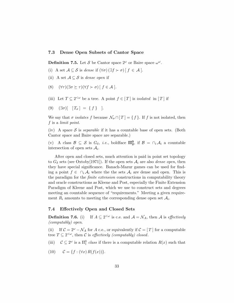
Definition 7.5. Let S be Cantor space 2ω or Baire space ωω.

(i) A set A ⊆ S is dense if (∀σ) (∃f � σ) [ f ∈ A ].

(ii) A set A ⊆ S is dense open if

(8) (∀τ)(∃σ � τ)(∀f � σ) [ f ∈ A ].

(iii) Let T ⊆ 2<ω be a tree. A point f ∈ [T ] is isolated in [T ] if

(9) (∃σ)[ [Tσ ] = { f } ].

We say that σ isolates f because Nσ ∩ [T ] = {f }. If f is not isolated, thenf is a limit point.

(iv) A space S is separable if it has a countable base of open sets. (BothCantor space and Baire space are separable.)

(v) A class B ⊆ S is Gδ, i.e., boldface Π02, if B = ∩iAi a countable

intersection of open sets Ai.

After open and closed sets, much attention is paid in point set topologyto Gδ sets (see Oxtoby[1971]). If the open sets Ai are also dense open, thenthey have special significance. Banach-Mazur games can be used for find-ing a point f ∈ ∩iAi where the the sets Ai are dense and open. This isthe paradigm for the finite extension constructions in computability theoryand oracle constructions as Kleene and Post, especially the Finite ExtensionParadigm of Kleene and Post, which we use to construct sets and degreesmeeting an countable sequence of “requirements.” Meeting a given require-ment Ri amounts to meeting the corresponding dense open set Ai.

7.4 Effectively Open and Closed Sets

Definition 7.6. (i) If A ⊆ 2<ω is c.e. and A = NA, then A is effectively(computably) open.

(ii) If C = 2ω −NA for A c.e., or equivalently if C = [T ] for a computabletree T ⊆ 2<ω, then C is effectively (computably) closed .

(iii) C ⊆ 2ω is a Π01 class if there is a computable relation R(x) such that

(10) C = {f : (∀x)R(f(x))}.

33

We call this lightface Π01 because it is defined in (10) by a universal quantifier

outside of a computable relation R(x).

(iv) A set C ⊆ 2ω is boldface Π1 if there is some set S ⊆ ω such that

C = {f : (∀x)RS(f(x))},

and we say C is in ΠS1 . Here RS denotes a relation computable in the set S

which we call the parameter determining RS . A set A ⊂ 2ω is boldface Σ1

or ΣS1 if its complement 2ω −A is boldface Π1 or ΠS

1 .

Theorem 7.7. The open (closed) sets of 2ω are exactly the boldface Σ1

(Π1) sets and any boldface set is lightface in some parameter A.

Proof. If A is open, then A = NA for some countable set A. Now A de-termines exactly which σ contribute in the countable union A = ∪σ∈A Nσ.Hence, if we fix A as a parameter, then the definition and properties becomelightface ΣA

1 , i.e., effectively open relative to the oracle A. (But this entiresection is about working relative to an oracle.)

We often convert an open set A = NA into the realm of computabilitytheory as follows. We: (1) usually fix the parameter A and do a constructionwhich is computable relative to the parameter A; (2) often replace the openset NA by its complement the closed set C = NA; and (3) replace the closedset by C = [TA ] for a A-computable tree T . By fixing the parameter A wecan apply all the methods of this chapter on A-computable constructions,such as the Recursion Theorem, construction of an A-c.e. set B, and soforth.

Theorem 7.8. A class C is a Π01 class iff C is effectively closed, i.e., C = [T ]

for some computable tree T .

Proof. (=⇒). Let C = { f : (∀x)R(f(x)) } for R computable. Define acomputable tree T = { σ : (∀τ ⊆ σ)[R(τ)] }. Then [T ] = C.

(⇐=). Let C = [T ] for T a computable tree. Define R(σ) iff σ ∈ T . Then{f : (∀x)R(f(x))} = [T ].

7.5 Continuous Functions on Cantor Space

In elementary calculus courses a continuous function is usually defined withδ and ε concepts or with limits. In advanced analysis or topology courses

34

the more general definition is presented that a function F is continuous iffthe image of every basic open set is open. We state continuity now forfunctionals on the Cantor space 2ω . For arbitrary topological spaces anopen set is an arbitrary union of basic open sets, but for Cantor space wemay take countable unions.

Definition 7.9. (i) A functional Ψ on Cantor space 2ω is continuous if forevery τ ∈ 2<ω there is a countable set Xτ such that

(11) Ψ−1 (Nτ ) = ∪ { Nσ : σ ∈ Xτ }.

By identifying string σy with code number y defined in Definition 7.1 (iii)we can think of Xτ as a subset of ω.

(ii) A functional Ψ on Cantor space 2ω is total if ΨA(x) is defined for everyA ⊆ ω and x ∈ ω, i.e., if (∀A)(∃B)(∀x)[ ΨA(x) = B(x) ].

Theorem 7.10. Let Ψ be a continuous functional on Cantor Space 2ω.Then Ψ is total iff for each set Xτ of (11) there is a finite subset Xτ ⊆ Xτ

such that,

(12) 2ω ⊆ ∪ { Nσ : σ ∈ Xτ }.

Proof. (⇐=). Given such Xτ for every τ we see that Ψ is total by (12).

(=⇒). Assume Ψ is total. Then for every τ there is a countable set Xτ

which covers 2ω in the sense of (12). Now the Compactness Theorem assertsthat any open cover of Cantor space 2ω has a finite subcover. Therefore, wecan replace every set Xτ by a finite subset Xτ .

Note that this involves only compactness and has no computable content,although it is usually presented in its effective analogue as the theorem thatΦe is total iff it is a truth-table reduction.

7.6 Effectively Continuous Functionals

A Turing functional Φe is not only continuous but effectively continuous inthe following sense.

Theorem 7.11. For Φe define for every τ ∈ 2<ω the set of strings

(13) Xeτ = { σ : (∃s)(∀x < |τ | ) [ Φσ

e,s(x)↓ = τ(x) ] }.

Then Xeτ is c.e. and uniformly so in the sense that there is a computable

function h(e, τ) such that Wh(e,τ) = Xeτ .

35

Proof. Use the Oracle Graph Ge. Identify string σ with Nσ. Now the set ofstrings {Xe

τ : τ ∈ 2ω } witnesses that the functional Φe is continuous.

Definition 7.12. Since Xeτ is not only countable but also computably enu-

merable uniformly in e the functional Φe is effectively continuous, i.e., thatXeτ is a computably enumerable set of strings.

7.7 Continuous Functions are Relatively Computable

We showed that any Turing functional is continuous, indeed effectively con-tinuous. Now we prove that any continuous functional on 2ω is a Turingfunctional relative to some real parameter X ⊆ ω and therefore is effectivelycontinuous relative to X.

Theorem 7.13. Suppose Ψ is a continuous functional on 2ω. Then Ψ is aTuring functional relative to some real parameter X ⊆ ω.

Proof. Since Ψ is continuous, the inverse image of every basic open set Nτ ,τ ∈ 2<ω, is open and therefore is a countable union of basic open sets.Hence, (identifying strings σ with their code numbers as integers) there is aset Xτ ⊆ ω such that,

Ψ−1 (Nτ ) = ∪ { Nσ : σ ∈ Xτ }.

Therefore, the set X = ⊕{Xτ : τ ∈ 2<ω} provides a complete oracle forcalculating Ψ : 2ω → 2ω.

8 Bounded Reducibilities

8.1 A Matrix Mx for Bounded Reducibilities

A bounded reducibility is a Turing reducibility ΦAe (x) with a computable

function h(x) which bounds the use function, i.e., ϕAe (x) ≤ h(x). Givenh(x) imagine a matrix Mx whose rows are all the strings σ of length h(x).The action on x is entirely determined by the action of Φσ

e (x) for these rowsσ ∈ Mx. For example, if B ≤m A via a computable function f(x) thenthis reduction is bounded by h(x) = f(x) and x ∈ B iff σ(f(x)) = 1 whereσ ≺ A, i.e., where σ is an initial segment of A. In Definition 7.1 (iii) wedefined σy to be the string with canonical index y derived from Dy. Thisgives a method for indexing the rows σy ∈Mx.

We begin in §8.2 with the most general bounded reducibility calledbounded Turing reducibility (B ≤bT A) where we are given only the com-putable bound h(x), i.e., only the matrix Mx. In §8.3 we study the more

36

restrictive case of truth-table reducibility (B ≤tt A) where Φσe (x) converges

for every x and every row σ ∈ Mx. If Φσe (x) diverges for even one x and

σ ∈Mx then the reduction is a partial bT-reduction, but if it converges forevery x and every σ ∈Mx then it gives a genuine truth-table as in beginninglogic courses as defined in Theorem 8.3 (iii). This convergence on all stringsσy ∈Mx is the key defining property for a tt-reduction as expressed in (14).

8.2 Bounded Turing Reducibility

Definition 8.1. (i) A set B is bounded Turing reducible (bT-reducible) toa set A (B ≤bT A) if there is a Turing reduction ΦA

e = B and a computablefunction h(x) such that the use ϕAe (x) ≤ h(x).

(ii) A set B is identity bounded Turing reducible to A (B ≤ibT A) if B ≤bT Awith h(x) = x.

The bT and ibT reductions occur naturally in several parts of the subject.For example, often we are given a noncomputable c.e. set A and we constructa simple set B ≤T A by simple permitting where an element x is allowed toenter B at stage some stage only if some y ≤ x has just entered A. WhenA�x has settled then B�x has settled also, and hence B ≤ibT A.

More recently, ibT has occurred in applications of computability to dif-ferential geometry in Soare [2004] and Csima-Soare [ta], as described later,and ibT reducibility has also been used in applications to algorithmic ran-domness and Kolmogorov complexity. Barmpalias and Lewis [ta] have shownthe nondensity of the ibT -degrees of c.e. sets.

8.3 Truth-Table Reductions

Definition 8.2. A set B is truth-table reducible to set a A (B ≤tt A) ifB ≤bT A via ΦA

e = B and h(x) as in Definition 8.1, and also

(14) (∀x)(∀σ)[ |σ| = h(x) =⇒ Φσe (x)↓ ].

Theorem 8.3. [Truth-Table Theorem, Nerode]. The following defi-nitions of tt-reducible are equivalent.

(i) B ≤tt A as defined in Definition 8.2 and (14).

(ii) ΦAe = B for some total ΦX

e that is (∀X)(∃Y )(∀x)[ ΦXe (x) = Y (x) ].

37

(iii) B ≤tt A via ΦAe and h(x) as in Definition 8.2. In addition, there is a

computable function g(x) such that

Dg(x) = { y : |σy| = h(x) & Φσye (x) = 1 }.

(iv) There exist computable functions g and h such that, for all x,

x ∈ B ⇐⇒ (∃z ∈ Dg(x) [ A�(h(x) + 1) = Dz ].

Proof. The implications (i) =⇒ (ii), (iii) =⇒ (i), and (iii) ⇐⇒ (iv) areobvious. It remains to prove (ii) =⇒ (iii).

(ii) =⇒ (iii). Uniformly in x we can effectively enumerate the set

Ux = { σ : Φσe (x)↓ }.

Since Φe is total apply the Compactness Theorem 7.4 (iv) to get a finitesubset Vx ⊆ Ux such that ∪{Nσ : σ ∈ Vx } ⊇ 2ω. Define h(x) and g(x) by

h(x) = max{ |σ| : σ ∈ Vx }.

Dg(x) = { y : |σy| = h(x) & Φσye (x) = 1 }.

Remark 8.4. Post [1944, §6] introduced the first definition of B ≤tt A.For every integer n he required a effective procedure to produce integersk, and m1,m2 . . .mk. He then drew a diagram of a matrix with columnsm1, . . . ,mk and 2k rows with individual entries of + for x ∈ A and − forx /∈ A. Letting h(x) be the maximum of the {mi}i≤k, filling in all columnsless than h(x), and replacing + by 1 and − by 0 we have exactly the matrixMx described in §8.1. Next Post drew a vertical line to the right of thismatrix and added an extra column such that an entry vz in this columnfollowing row Rz indicated that if A satisfies row Rz then x ∈ B iff vz = +.

Post’s extra column converted the matrix Mx into a total reductionbecause A had to extend exactly one of the rows Rz and then the valuefor B(x) was completely specified by vz given in advance. Therefore, Post’soriginal definition [1944] of B ≤tt A is virtually identical in intuition anddescription to our Definition 8.2 above where we could attach to matrixMx an extra column with the value Φσ

e (x) on row σ. In both cases thecrucial point is that Φσ

e (x) is defined for every string of length h(x) beforeexamining the oracle A. Property (iv) of B ≤tt A has been used in the

38

past e.g., Soare [1987, p. 83] and is short and slick but is does not give thenecessary elegance and intuition for beginning students.

Turing reducibility was not well understood in 1944 and an understand-ing of it in its modern state emerged only gradually during the 1940’s and1950’s. Post’s tt-reducibility in 1944 was understood at once. Therefore,in 1959 Friedberg and Rogers introduced wtt-reducibility (B ≤wtt A) asa weakening of tt-reducibility which was already a strengthening of ≤T.Therefore, the concept of wtt has distance two from the central concept ≤T.The concept of bounded Turing reducibility (bT), which has the same defini-tion as wtt, goes immediately to the main concept of bounding the queriedinformation by a computable function h(x). Thus, ≤bT has distance onefrom the main reducibility of ≤T. The concept of tt-reducibility is tied tothe totality of the reduction ΦA

e which is exactly what bT-reducibility lacks.Also bT is more recognizable than wtt whose meaning cannot be guessedfrom its name.

8.4 Difference of c.e. sets, n-c.e., and ω-c.e. sets

The Limit Lemma characterized sets A ≤T ∅′ as those such that A = limsAsfor a computable sequence {As}s∈ω. Now consider special cases based uponhow many times the approximation changes on x. These notions are moregeneral than c.e. sets A but not the most general case of A ≤T ∅′.

Definition 8.5. (i) A setD is the difference of c.e. sets (d.c.e.) ifD = A−Bwhere A and B are c.e. sets.

(ii) The set A is omega-c.e. (written ω-c.e.) if there is a computable sequence{As}s∈ω with A0 = ∅ and a computable function g(x) which bounds thenumber of changes in the approximation {As}s∈ω in the following sense,

(15) A = limsAs & | { s : As(x) 6= As+1(x) } | ≤ g(x).

(iii) For n ∈ ω the set A is n-c.e. if g(x) ≤ n.

For example, the only 0-c.e. set is ∅, the 1-c.e. sets are the usual c.e. sets,and the 2-c.e. sets are the d.c.e. sets. The next theorem gives an elegantcharacterization of ω-c.e. sets.

Theorem 8.6. The following are equivalent.

(i) A ≤bT ∅′.(ii) A is ω-c.e.

(iii) A ≤tt ∅′.

39

Proof. Clearly, (iii) implies (i).

(i) =⇒ (ii). Suppose Φ∅′e = A with computable bound g(x) ≥ ϕ∅′e (x). Let

As(x) = Φ∅′e (x)[ s ] where we may speed up the computation so the latter is

always defined. Now As+1(x) 6= As(x) only if some element z ≤ g(x) enters∅′ which can happen at most g(x) + 1 times, once for each z ∈ [0, g(x)].

(ii) =⇒ (iii). Assume A = limsAs satisfies (15) via g(x). Define the c.e.change set C by

C = { 〈k, x〉 : 1 < k ≤ | {s : As(x) 6= As+1(x)} | }.

(Intuitively, whenever As(x) 6= As+1(x) we put into C the least elementof the form 〈k, x〉, i.e., on row ω[x], not already in C.) Therefore, |C [x]| isthe number of changes on x during the approximation, and |C [x]| ≤ g(x)by hypothesis (ii). Furthermore, A(x) = 1 iff |C [x]| is odd, because theapproximation changes between 0 and 1 starting with 0.

First build a truth-table to demonstrate that A ≤tt C. For a given xthe truth-table has rows of width g(x) as in Definition 8.2 (ii). For eachk ≤ g(x) construct a row beginning with k many 1′s followed by all 0′s.Now to tt-compute from C whether x ∈ A compute k = |Cx|. Next find therow with k many 1’s. Now A(x) = 1 iff k is odd. Hence, A ≤tt C. However,C is c.e. Hence, C ≤m 0′ and therefore A ≤tt 0′.

This result shows the difference between T -reductions and tt-reductions.First, the assumption on h(x) ensures that A ≤bT D. Second, the approx-imation always begins with As(x) = 0 for s = 0 and changes between 0and 1 because all values are in {0, 1} rather than in ω. Therefore, we canmake up a row in the truth-table which gives value for A(x) based only onthe number of changes. This ensures that A ≤tt D. This case is unusualsince most reductions we consider only produce A ≤T B for some set B andsometimes produce A ≤bT B as in permitting arguments.

9 Online Computing

The original implementations of computing devices were generally offlinedevices such as calculators or batch processing devices. However, in recentyears the implementations have been increasingly online computing deviceswhich can access or interact with some external database or other device.The Turing o-machine is a better model to study them because the Turinga-machine lacks this online capacity.

40

Definition 9.1. (i) An online or interactive computing process is one whichinteracts with its environment, for example a computer communicating withan external data base such at the World Wide Web.

(ii) An offline computing process is one which begins with a program andinput data, and proceeds internally, not interacting with any external device.This includes a calculator, and batch processing devices where a user handeda deck of punched IBM cards to an operator, who fed them to the computerand produced paper output later.

There are many descriptions in the computing literature about onlineand interactive processes. In [Goldin-Smolka-Wegner] a chapter by YuriGurevich, Interactive Algorithms 2005 is described,

“In this chapter, Gurevich asserts that computer science is largelyabout algorithms, and broadens the notion of algorithms to in-clude interaction by allowing intra-step interaction of an algo-rithm with its environment.”

About the chapter, A Theory of Interactive Computation by Jan vanLeeuwen and Jiri Wiedermann, the book states,

“This chapter asks what a computational theory of interactive,evolving programs should look like. The authors point out that atheory of interactive computation must necessarily lead beyondthe classical, finitary models of computation. A simple model ofinteractive computing is presented consisting of one componentand an environment, interacting using single streams of inputand output signals.”

It appears that the Turing o-machine is a good theoretical model toanalyze an interactive process because there is usually a fixed algorithmor procedure at the core, which by Turing’s thesis we can identify with aTuring a-machine, and there is a mechanism for the process to communicatewith its environment, which when coded into integers may be regarded asa Turing type oracle. Under the Post-Turing Thesis 6.1 these real worldonline or interactive processes can be described by a Turing oracle machine.

In real world computing the oracle may be called a database or an en-vironment. A laptop obtaining data from the World Wide Web is a goodexample. In the real world the database would not be literally infinite butmay appear so (like the web) and is usually too large to be convenientlydownloaded into the local computer. Sometimes the local computer is calledthe “client” and the remote device the “server.”

41

9.1 Turing Machines and Online Processes

We could continue analyzing to what extent Turing oracle machines canmodel modern online processes, but let us now examine the reverse direction,that o-machines are online while a-machines are not. The following pointsappear self-evident.

• Turing oracle machines are online. An o-machine has fixed programbut has the capacity to interact with its environment and receive newdata during its computation.

• The original Turing a-machines are not online. A Turing a-machine,even a universal machine, begins with a fixed program and fixed inputand proceeds without further outside input until (if ever) it halts.

• A large number and rapidly increasing number of computing processesin the real world are online or interactive. See the authors in [Goldin-Smolka-Wegner] for only a few.

• A large number of books presenting an introduction to computabilitymention Turing oracle machines and relative computability very latein the book or not at all.

• A large number of books with articles on Turing and the Church-Turing Thesis do not mention Turing oracle machines or relative com-putability at all, e.g., Christof Teuscher [2004].

Discussing only Turing a-machines in modern texts, or only the Church-Turing Thesis, and not the Post-Turing Thesis on oracle computers, is likediscussing only batch processing machines of the 1950’s long after the emer-gence of online computing.

9.2 Trial and Error Computing

We expect Turing a-machines and o-machines to be absolutely correct. How-ever, there are many computing processes in the real world which give a se-quence of approximations to the final answer. Turing considered machineswhich make mistakes. In his talk to the London Mathematical Society,February 20, 1947, quoted in Hodges, p. 360–361, Turing said,

“I would say that fair play must be given to the machine. Insteadof it sometimes giving no answer we could arrange that it gives

42

occasional wrong answers. But the human mathematician wouldlikewise make blunders when trying out new techniques. It iseasy for us to regard these blunders as not counting and give himanother chance, but the machine would probably be allowed nomercy. In other words if a machine is expected to be infallible, itcannot also be intelligent. There are several theorems which sayexactly that. But these theorems say nothing about how muchintelligence may be displayed if a machine makes no pretence atinfallibility.

Hillary Putnam [1965] described trial and error predicates as ones forwhich there is a computable function which arrives at the correct answerafter a finite number of mistakes. In modern terminology this is calleda limit computable function as described in Soare [1987] or Soare [CTA]Chapter 3. This is a model for many processes in the real world which allowfinitely many mistakes but gradually move closer to the correct answer.

9.3 The Limit Lemma

There are several different approaches for computing with finite errors.

Definition 9.2. A computable sequence of computable sets {Bs}s∈ω is acomputable (∆0) approximating sequence for a set B if B = limsBs. If thereis such a sequence we say that B is limit computable,

Lemma 9.3. [Limit Lemma, Shoenfield, 1959]. The following areequivalent.

(i) B ≤T A for some c.e. “oracle set” A.

(ii) B is limit computable.

(iii) B ∈ ∆2, that is, B is is both two quantifier forms.

Proof. (See Soare [1987] or Soare [CTA] Lemma 3.3.6.)

Now in the real world imagine an example of a computing process witherror such as: a robot learning a maze; a financial trader receiving informa-tion from around the world updated every second; a meteorologist predictingthe weather a week from now given constantly updated weather conditionstoday. In our idealized model we assume that the individual makes finitelymany errors during the process {Bt}t∈T for time periods t ∈ T but even-tually gets the correct answer. (In practice, the final answer may not be

43

exactly correct in these examples, but is presumably more accurate thanthe first approximation B0. The sequences of improving approximations,even if not exact, are usually useful in financial trading, meteorology, andother approximations in real time.)

9.4 Two Models for Computing With Error

9.4.1 The Limit Computable Model

In the limit computable or approximation model we have a sequence ofTuring programs {Pt : t ∈ T} so that Pt computes function gt at time t ∈ T .There is not necessarily any connection between different programs and wemay have to compute all over again with a new program as we pass fromtime t to t+ 1.

Suppose the financial trader in Chicago receives data every second t ∈ Tabout currency prices in London, Milan, New York and Tokyo. The config-uration at his trading desk may be described using the Limit Lemma by acomputable function where gt is the computable characteristic function ofBt, the configuration of his computation at the end of time t. The com-putable function gt gives an algorithm to compute the condition Bt at timet but it gives no relationship between Bt and Bt+1. It will not be possiblefor the trader to write a new program every second. How will the traderwrite a program to uniformly compute the index gt for t ∈ T?

9.4.2 The Online Model

By the Limit Lemma there is a c.e. set A (or even a ∆02 set) and oracle

machine Φe such that B = ΦAe . Now the trader can program the algorithm

Φe into his laptop once and for all at the start of the trading day. Everysecond t ∈ T he receives from New York and abroad the latest quotes Atwhich enter directly into his computer by an internet connection. He doesnot (and cannot) change the program Φe every second. His algorithm simplyreceives the “oracle” information At from the internet as it is continuallyupdated, and computes the approximation Bt(x) = ΦAt

e (x). His programthen executes a trade when the algorithm determines that conditions arefavorable. It is difficult to see how this trader could have carried out hisbusiness using a batch processing, Turing a-machine model, instead of anonline model.

44

10 Three Displacements in Computability Theory

The dictionary defines “displacement” to be the moving of something fromits rightful place or position, often when replaced by something else. Thereare three important issues in computability which have at one time beendisplaced from their correct or proper positions as evaluated by historicaland scientific criteria. These issues are at the very heart of the subjectand they define how we think about computability. We now examine thesethree issues one by one in the next three sections. These items may havebeen displaced accidentally or without conscious thought or decision, simplyacting from the exigencies of the situation at the time, but are not consistentwith a careful scientific analysis later.

When computabiliy theory originated in the 1930’s it was a very smallfield attempting to consolidate its ideas. Furthermore, three of its leaders,Godel, Turing, and Church effectively left the field after 1940 and had littledirect influence thereafter on its development, although Church supervisedthe Ph.D. theses of many prominent researchers in the field. After 1940the field was developed and promulgated primarily by Stephen C. Kleenewith some additional influence by Emil Post as described earlier. In dedicat-ing his book Degrees of Unsolvability [1971] Shoenfield recognized Kleene’soverwhelming influence,

“Dedicated to S.C. Kleene who made recursive function theoryinto a theory.”

This is entirely accurate and without Kleene’s leadership we would not havethe field as we know it today. However, a number of changes took place after1940, perhaps by accident, that were not consistent with the original devel-opment of computability in the 1930’s and would not have been approvedof by Godel and Turing.

11 “Computable” versus “Recursive”

Starting in 1936, Church and Kleene used the term “recursive” to mean“computable” even though Turing and Godel later objected. Kleene laterintroduced the term “recursive function theory” for the subject althoughGodel disagreed (see below). This was the first time in history that theterm “recursive” which had meant roughly “inductive” acquired the addi-tional meaning “computable” of “calculable.” After 1996 the term the term‘recursive” was again used only to mean “inductive” not “computable” or

45

“calculable.” From 1931 to 1934 Church and Kleene had used the λ-definablefunctions as the formal equivalent of effectively calculable functions, andChurch had first proposed his thesis privately to Godel in that form.

11.1 Church Defends Church’s Thesis with “Recursive”

Recall Church’s Thesis 2.1 (First Version) [1934] “A function is effectivelycalculable if and only if it is λ-definable.” When Godel strongly rejected tothis thesis Church turned instead to Godel’s own Herbrand-Godel generalrecursive functions as a formalism and proposed in [1935] and [1936] thewell-known form of his thesis, Church’s Thesis 2.2 [1936] A function on thepositive integers is effectively calculable if and only if it is recursive.

Church and Kleene knew almost immediately and published by 1936the proof of the formal equivalence of recursive functions with λ-definablefunctions. After seeing Godel’s lectures in 1934 Church and Kleene droppedthe λ-definable functions and adopted the recursive functions. This wasnot because of the inadequacy of λ-definable functions in comparison to therecursive functions. Indeed Church seems to have preferred the λ-definablefunctions and caused Turing to write his thesis [1939] in that formalism.

Church was very eager for mathematicians to accept his thesis and heknow that the recursive functions were more familiar to a mathematical au-dience than λ-definable ones. Church and Kleene used the second versionof Church’s Thesis above, phrased in terms of recursive functions primarilyfor public relations as Kleene [1981] explained, “I myself, perhaps undulyinfluenced by rather chilly receptions from audiences around 1933–35 to dis-quisitions on λ-definability, chose, after general recursiveness had appeared,to put my work in that format. . . . ” Church and Kleene were simply doingwhat most scientists do, arrange the work in a framework which will beunderstandable and appealing to as large a scientific audience as possible.Ironically, this is exactly what caused the change in 1996 from “recursive”back to “computable” because in 1996 the term “computable” was muchbetter understood by a general audience than “recursive.” The irony is thatthe term “computable” was there all along and was preferred by Turing andGodel.

11.2 Church and Kleene Define “Recursive” as “Computable”

By 1936 Kleene and Church had begun thinking of the word “recursive”to mean “computable.” Church had seen his first thesis rejected by Godeland was heavily invested in the acceptance of his 1936 thesis in terms of

46

recursive functions. Without the acceptance of this thesis Church had nounsolvable problem. Church wrote in [1936, p. 96] printed in Davis [1965]that a “recursively enumerable set” is one which is the range of a recursivefunction. This is apparently the first appearance of the term “recursivelyenumerable” in the literature and the first appearance of “recursively” asan adverb meaning “effectively” or “computably.”

In the same year Kleene [1936, p. 238] cited in Davis [1965] [p. 238]mentioned a “recursive enumeration” and noted that there is no recursiveenumeration of Herbrand-Godel systems of equations which gives only thesystems which define the (total) recursive functions. By a “recursive enu-meration” Kleene states that he means “a recursive sequence (i.e., the suc-cessive values of a recursive function of one variable).” Post [1944], underthe influence of Church and Kleene, adopted this terminology of “recursive”and “recursively enumerable” over his own terminology [1943], [1944] of “ef-fectively generated set,” “normal set,” “generated set.” Thereafter, it wasfirmly established.

11.3 Godel Rejects “Recursive Function Theory”

Neither Turing nor Godel ever used the word “recursive” to mean “com-putable.” Godel never used the term “recursive function theory” to namethe subject; when others did Godel reacted sharply negatively, as related byMartin Davis.

In a discussion with Godel at the Institute for Advanced Study inPrinceton about 1952–54, Martin Davis casually used the term“recursive function theory” as it was used then. Davis related,“To my surprise, Godel reacted sharply, saying that the term inquestion should be used with reference to the kind of work RoszaPeter did.”

(See Peter’s work on recursions in [1934] and[1951].) By 1990 the situationhad become very difficult. Most people access to a personal computer ontheir desks and the terms of computing were familiar to the general popula-tion but “recursive” was limited to very small number who mainly associatedit with a first year programming course or a definition by induction on math-ematics and almost never with computability. So few people understood themeaning of “recursive” that by 1990 I had to begin my papers with,

“Let f be a recursive function (that is, a computable function),”

as if I were writing in Chinese and translating back into English.

47

11.4 The Ambiguity in the Term “Recursive”

The traditional meaning of “recursive” as “inductive” led to ambiguity.Kleene often wrote of calculation and algorithms dating back to the Baby-lonians, the Greeks and other early civilizations. However, Kleene [1981b,p. 44] wrote,

“I think we can say that recursive function theory was bornthere ninety-two years ago with Dedekind’s Theorem 126 (‘Satzder Definition durch Induktion’) that functions can be definedby primitive recursion.”

Did he mean that recursion and inductive definition began with Dedekind orthat computability and algorithms began there? The latter would contradicthis several other statements, such as Kleene [1988, p. 19] where he wrote,“The recognition of algorithms goes back at least to Euclid (c. 330 B.C.).”When one uses a term like “recursive” to also mean “computable” or “algo-rithmic” as Kleene did, then one is never sure whether a particular instancemeans “calculable” or “inductive” and our language has become indistinct.Returning “recursive” to its original meaning of “inductive” has made itsuse much clearer. We do not need another word to mean “computable.” Wealready have one.

11.5 Changing “Recursive” Back to “Inductive”

By 1996 the confusion had become intolerable. I wrote an article on Com-putability and Recursion for the Bulletin of Symbolic Logic [1996] on thehistory and scientific reasons for why we should use “computable” and not“recursive” to mean “calculable.” “Recursive” should mean “inductive” asis had for Dedekind and Hilbert. At first few were willing to make such adramatic change, overturning a sixty year old tradition of Kleene, and thewords “computability theory” and “computably enumerable (c.e.) set” didnot come tripping from the lips. However, in a few months more peoplewere convinced by the undeniable logic of the situation. Three years laterat the A.M.S. conference in Boulder, Colorado referenced in Soare [2000],most researchers, especially those under forty years old, had adopted thenew terminology and conventions. Changing back from from “recursive” to“computable” during 1996–1999 has had a number of advantages.

Historical Accuracy. The founders of the two key models of com-putabilty, Turing and Godel, had never used “recursive” to mean com-putable and indeed had objected when it was so used. The object of

48

everyone was to formally capture the informal concept of “effectivelycalculable” which Turing machines did to Godel’s satisfaction, whileat first Godel’s own model of Herbrand-Godel recursive functions didnot. The object was never to understand the notion of recursionsor inductive definitions. In 1935 Church adopted Godel’s recursivefunctions as a definition of effectively calculable before seeing Turingmachines As Kleene relates, Church and Kleene did this as a matterof public relations to relate to a concept mathematicians could under-stand, not in an attempt to better understand the nature of recursionand inductive definition.

Scientific Accuracy. The words “calculate” and “compute” are veryclose in the dictionary, the former being a bit more general. Theword “recursive” means a procedure characterized by recurrence orrepetition from the Latin verb “recurrere,” to run back. The wordhas nothing to do with “calculate” or “compute.” The general publicunderstands the first two words in this context. To the extent that theyhave any idea about “recursive” they understand it in this context.For example, a first year programming course speaks of definition byiteration versus definition by recursion.

Name Recognition. Suppose a student is scanning a catalogue for acourse to take and sees the course title “Recursive Function Theory”versus “Computability Theory.” Which will give him more informationabout the content of the course? Should a fresh Ph.D. apply for jobsunder the general area of his work as the first or second? Should aprofessor write an abstract for his lecture at another university underthe first title or second?

Names do matter. They mattered to Church and Kleene in 1936 whenthey changed from the term “λ-definable function” to “recursive function”to achieve greater name recognition among mathematicians and to makeChurch’s Thesis more convincing before the appearance of Turing. Namesmatter today as we try to relate our specialty of computability to the worldof computers and algorithmic procedures all around us, a world partiallycreated by Turing.

49

12 Renaming it the “Computability Thesis?”

12.1 Kleene Called it “Thesis I” in [1943]

In the 1930’s both Church and Turing thought they were giving definitionsof an effectively calculable function, not putting forth a “thesis.” These werenot even called “theses” at all until Kleene [1943, p. 60] referred to Church’s“definition” as “Thesis I.”

12.2 Kleene Named it “Church’s thesis” in [1952]

Later in his very influential book [1952] it is fascinating to see how Kleene’sthinking and terminology progressed from “Thesis I” to “Church’s Thesis”and not to “Turing’s Thesis” or the “Church-Turing Thesis.” Kleene [1952,p. 300] took up where Kleene [1943] had left off.

“This heuristic evidence and other considerations led Church1936 to propose the following thesis.

Thesis I. Every effectively calculable function (effectively decid-able predicate) is general recursive.”

This is identical with what we previously called Church’s Thesis 2.2. Ofcourse, Kleene was aware of other similar “theses” advanced nearly simul-taneously and he continued [1952, p.300],

“This thesis is also implicit in the conception of a computingmachine formulated by Turing 1936–7 and Post 1936.”

Next Kleene begins a subtle shift of terminology from “Thesis I” to“Church’s thesis.” Apparently he did not feel it necessary to include Turing’sname when he used the term “Church’s thesis.” Kleene wrote [1952, p.317]began a new section §62 and called it “Church’s thesis” instead of “Thesis I”as he had been doing. Kleene wrote,

“ §62. Church’s thesis. One of the main objectives of this andthe next chapter is to present the evidence for Church’s thesis(Thesis I) §60.”

50

12.3 Kleene Dropped “Thesis I” for “Church’s thesis”

As Kleene progressed through [1952, §62, pp. 318–319] he dropped any ref-erence to “Thesis I” and used only “Church’s thesis” with no mention ofTuring or Post in the thesis. He wrote [1952, p. 318–319],

“ Church’s thesis, by supplying a precise delimitation of all ef-fectively calculable functions, . . . ”

“While we cannot prove Church’s thesis, since its role is to de-limit precisely an hitherto vaguely conceived totality, we requireevidence that it cannot conflict with the intuitive notion whichit is supposed to complete; . . . ”

“The converse of Church’s thesis, i.e., that every general recur-sive function ϕ is effectively calculable, we take to be alreadyconfirmed by the intuitive notion (cf. §60).”

12.4 Evidence for the Computability Thesis

In one of the most familiar parts of the book, Kleene summarized the ev-idence for “Church’s thesis” in [1952, §62, p. 319]. These arguments havebeen cited in hundreds of computability books and papers for the last halfcentury. After some heuristic evidence in (A), Kleene presented perhapsthe most powerful evidence, the “(B) Equivalence of diverse formulations:”such as the (Herbrand-Godel) general recursive functions, λ-definable func-tions, Turing computable functions, and systems of Post [1943] and [1946] ofcanonical and normal systems. Ironically, to clinch the evidence for Church’sthesis Kleene began a new part (C) where he appealed to Turing’s work andwrote,

“(C) Turing’s Concept of a Computing Machine.”

Turing’s computable functions [1936–7] are those which can becomputed by a machine of a kind which is designed, accordingto his analysis, to reproduce all sorts of operations which a hu-man computer could perform, working according to preassignedinstructions. Turing’s notion is thus the result of a direct at-tempt to formulate mathematically the notion of effective calcu-lability, while other notions arose differently and were afterwardsidentified with effective calculability. Turing’s formulation henceconstitutes an independent statement of Church’s thesis.”

51

We see here the amalgamation of different meanings into a single term(just as for “recursive” above). Kleene here was using the term “Church’sthesis” to include Turing’s Thesis and Turing’s justification. Turing’s workwas to establish the connection between effectively calculable functions andTuring computable functions in Turing’s Thesis 3.1. As an intensionalclaim it had nothing to do with the recursive functions of Church’s The-sis 2.2. It was only the equivalence of Turing computable functions firstwith λ-definable functions and hence with recursive functions which linksthem extensionally but not intensionally.

Remark 12.1. [The Computability Thesis Emerges]. It is exactlyhere that Kleene introduces (without explicit mention) another conventionand term which has lasted until today. Kleene knows that the various for-mal definitions all coincide extensionally, and he regards them interchange-ably, regardless of their intensional or historical import. From now on whenKleene uses the term “Church’s thesis” he means the following “Computabil-ity Thesis.” Kleene omits Turing’s name from the thesis even though in part(C) above he gave Turing credit as the only one who made a “direct attemptto formulate mathematically the notion of effective calculability.”

Definition 12.2. [The Computability Thesis]. A function on the pos-itive integers is effectively calculable if and only if it is recursive or Turingcomputable, or defined by any of the other formalisms.

Note that the Computability Thesis is essentially the same as what wehave called the Church-Turing Thesis 3.2. It does not refer to one single manor to one single formalism. The Computability Thesis, used extensively inthe subject, is usually listed under the name “Church’s Thesis” as in thetitle of the new book [Olszewski, 2007] with no mention of Turing. Manypeople today use “Church’s Thesis” in this way.

12.5 Who First Demonstrated the Computability Thesis?

Demonstrating something like the Computability Thesis requires two steps.

The Formalism. A formal mathematical definition for effectively calcula-ble functions. Church [1936] proposed Godel’s general recursive func-tions [1934]. Turing invented the new formalism of Turing machinesbecause this was closest to his idea of a mechanical process and be-cause it lent itself to proving that any effectively calculable functionlay in this class.

52

The Demonstration. The second and perhaps more important step is toprove that the informal notion of a person calculating a function can besimulated by the formal model. This step is not a purely mathematicalone but it needs to be as convincing and logical as possible. We referto this step as a “demonstration” rather than a formal “proof.”

Although it is not a formal proof, this second step is so crucial that it hasbeen referred to as a “theorem” by Gandy and others. Gandy [1988, p. 82]observed, “Turing’s analysis does much more than provide an argument for‘Turing’s Thesis,’ it proves a theorem.”3 Furthermore, as Gandy [1988,pp. 83–84] pointed out, “Turing’s analysis makes no reference whatsoever tocalculating machines. Turing machines appear as a result, a codification, ofhis analysis of calculations by humans.” Turing’s Thesis [1936, §9] statedin Definition 3.1 is that every intuitively computable (effectively calculable)function is computable by a Turing machine.

In contrast, Church used the Herbrand-Godel general recursive functionsas his formal model but even their inventor, Godel, was not convinced aswe have seen in §2 and §3. No modern book uses the H-G general recursiveformalism to define the effectively calculable functions.

A considerably more serious objection is that there was a flaw in Church’sdemonstration that every effectively calculable function is general recursive.The flaw in Church’s argument [1936, §7] for his thesis was this. Churchbegan by defining an “effectively calculable” function to be one for which“there exists an algorithm for the calculation of its values.” Church analyzedthe informal notion of the calculation of a value f(n) = m according to astep-by-step approach (so called by Gandy [1988, p. 77]) from two points ofview, first by an application of an algorithm, and second as the derivation insome formal system, because as he pointed out, Godel had shown that thesteps in his formal system P were primitive recursive. Following Davis [1958,p. 64] or Shoenfield [1967, pp. 120–121] it is reasonable to suppose that thecalculation of f proceeds by writing expressions on a sheet of paper, andthat the expressions have been given code numbers, c0, c1, . . . cn. Define〈c0, c1, . . . cn〉 = pc00 · p

c11 . . . pcnn . We say that the calculation is stepwise

recursive if there is a partial recursive function ψ such that ψ(〈c0, . . . , ci〉) =ci+1 for all i, 0 ≤ i < n.

3Gandy actually wrote “Church’s thesis” not “Turing’s thesis” as written here, butsurely Gandy meant Turing’s Thesis, i.e., the computability thesis, at least intensionally,because Turing did not prove anything in [1936] or anywhere else about general recursivefunctions.

53

If the basic steps are stepwise recursive, then it follows easily by theKleene Normal Form Theorem which Kleene had proved and communicatedto Godel before November, 1935 (see Kleene [1987b, p. 57]), that the entireprocess is µ-recursive. The fatal weakness in Church’s argument was thecore assumption that the atomic steps were stepwise recursive, somethinghe did not justify. Gandy [1988, p. 79] and especially Sieg [1994, pp. 80, 87],in their excellent analyses, brought out this weakness in Church’s argument.Sieg [p. 80] wrote, “. . . this core does not provide a convincing analysis:steps taken in a calculus must be of a restricted character and they areassumed, for example by Church, without argument to be recursive.” Sieg[p. 78] wrote, “It is precisely here that we encounter the major stumblingblock for Church’s analysis, and that stumbling block was quite clearly seenby Church,” who wrote that without this assumption it is difficult to seehow the notion of a system of logic can be given any exact meaning at all.It is exactly this stumbling block which Turing overcame by a totally newapproach.

12.6 The Computability Thesis and the Calculus

Why all the fuss over names? Why not simply use the term “Church’sThesis” invented by Kleene [1952], and let it refer to the “ComputabilityThesis?” This is in fact what is widely (and incorrectly) done.

If we had to attach a single name to “the calculus” every time we men-tioned it, whose name should it be? Isaac Newton began working on a formof the calculus in 1666 but did not publish it until much later. GottfriedLeibniz began work on the calculus in 1674 and published his account of thedifferential calculus in 1684 and the integral calculus in 1686. Newton didnot publish it until 1687 although most believe he had been working on itbefore Leibniz began in 1674. There was a great controversy about priorityup until Leibniz’s death in 1716. The British Royal Society handed downa verdict in 1715 crediting Isaac Newton with the discovery of the calculus,and stating that Leibniz was guilty of plagarism (although these chargeswere later proved false). Newton was more established than Leibniz andhad vigorous supporters. Newton and his followers campaigned vigorouslyfor his position. The Wiki encylopedia wrote,

“Despite this ruling of the Royal Society, mathematics through-out the eighteenth century was typified by an elaboration of thedifferential and integral calculus in which mathematicians gen-erally discarded Newton’s fluxional calculus in favor of the newmethods presented by Leibniz.”

54

12.7 Founders of Computability and the Calculus

There is a parallel between the development of the Calculus and the demon-stration of the Computability Thesis.

1. Church and Turing both worked independently on it and came up withdifferent models.

2. Turing began slightly later than Church. Leibnitz began later thanNewton. Both Leibniz and Turing worked at a distance and indepen-dently of Newton and Church, respectively, unaware of the work byanother researcher.

3. Turing’s model of Turing machines is overwhelmingly more appealingand popular that Church’s model of the (Herbrand-Godel) generalrecursive functions, a model which is rarely presented in any booksand never used for actual calculations in any courses. The generalrecursive functions are used only in an historical discussion. (Thisrefers to the Herbrand-Godel general recursive functions. The Kleeneµ-recursive functions have other uses but are were not mentioned inthe original Church’s Thesis 2.2.)

4. For the calculus, despite the Royal Society ruling, “mathematiciansgenerally discarded Newton’s fluxional calculus in favor of the newmethods presented by Liebniz.”

5. In computer science, the Turing machines (and other calculating ma-chines like register machines) dominate. The general recursive func-tions are never seen. Kleene’s µ-recursive functions are sometimesused in courses and mistakenly called recursive functions but to provethat an effectively calculable function is µ-recursive requires a tediousarithmetization as in Godel’s incompleteness theorem [1931] and isvirtually never done.

6. Newton was in the position of power with the Royal Society whichnot only affirmed his claim but denied the claim by his rival Leibniz.Church was the senior figure in computability (after Godel). Church’sclaim to the Computability Thesis was affirmed by his former Ph.D.student Stephen Kleene [1952]. Kleene occasionally mentioned Tur-ing’s Thesis and repeatedly used the Turing machine model and Tur-ing’s demonstration of its success to demonstrate the ComputabilityThesis. However, Kleene deliberately and overwhelmingly established

55

the phrase “Church’s thesis” to stand for the “Computability Thesis, ”at a time when nobody called it a thesis and when the field was aboutto rapidly expand in the 1950’s and 1960’s and would turn to Kleenefor direction as the last representative of the original computabilityresearchers of the 1930’s and the most prominent and influential ofall computability theorists in the 1950’s. The Royal Society was notsuccessful in excluding Leibniz from the calculus, but Kleene was cer-tainly successful in excluding Turing’s name from the ComputabilityThesis.

Virtually all the papers and books including Rogers [1967] and Soare[1987] and many others followed Kleene’s lead. Unlike the calculus, theparticipants, Church, Turing, and their followers, have given credit to theothers. The problem is simply that Kleene has not given Turing credit inhis naming of the Computability Thesis. Kleene could have called it “theComputability Thesis” analogously with “the calculus.” We never refer to“the Newton calculus” or the “Leibniz calculus.” Why do we need to givea person’s name to the Computability Thesis? Kleene never denied creditto Turing and in many places such as his books [1952] and [1967] he givesTuring credit for the most intuitive presentation of computability. Kleenejust does not include Turing in the name he chose.

Remark 12.3. Kleene thought and wrote with tokens, words that are givenarbitrary and nonstandard meaning by the author: “recursive” means “com-putable,” “Church’s Thesis” means the “Computability Thesis.” The arbi-trary and sometimes misleading use of words has diminished our communi-cations among ourselves and with other scientific and scholarly colleagues.

It is ambiguous to use “recursive” with both meanings, inductive andcomputable, as we have seen. Second, it is simply wrong to use “Church’sThesis” to refer to a proposition first demonstrated by Turing and neversuccessfully demonstrated by Church. It would also be wrong to refer to“the Newton Calculus” without mentioning Leibniz. Today we refer to “thecalculus” without any founder’s name. Why not call it simply, “the Com-putability Thesis” and not “Church’s Thesis,” or the “Church-Turing The-sis?” Which of the three terms is more understandable to an outsider whohas never heard about the subject?

56

13 Turing a-machines versus o-machines?

13.1 Turing, Post, and Kleene on Relative Computability

In §4 we have seen how Turing [1939, §4] briefly introduced an oracle machine(o-machine) and how and in §5–§7 how Post developed relative computabil-ity through the influential Kleene-Post [1954] paper. Kleene [1952, p. 314]took up the theme of relative computabilty of a function from an oracleset. Analogous to his version of Thesis I considered above, Kleene definedThesis I* to be the corresponding relative computability thesis which wehave called Post-Turing Thesis 6.1. He recommended this thesis but did notgive a separate justification. Kleene [1952, p. 314] wrote, “The evidence forThesis I will also apply to Thesis I*,” and on [1952, p. 319] he wrote,

“We now summarize the evidence for Church’s Thesis (and The-sis I*, end §61) under three main headings (A)–(C), and oneother (D) which may be included under (A).”

13.2 Relative Computability Unifies Incomputability

The field of computability theory deals mostly with incomputable not com-putable objects. The objects considered in degrees of unsolvability, in com-putable model theory, in differential geometry as in Csima-Soare [2006] orSoare [2004] all deal with incomputable objects. However, we should notcall the subject “incomputability theory” because the underlying theme isthe notion of relative computability as absolute because of the Oracle GraphTheorem 4.5, and because it relates and unifies the myriad incomputableobjects.

13.3 The Key Concept of the Subject

The notion of an oracle machine and relative computability is the singlemost important in the subject.

1. A Turing a-machine can easily be simulated by a Turing o-machineand the latter is scarcely more complicated to explain.

2. Most of the objects considered in computability theory and applica-tions to algebra, model theory, geometry, analysis and other fields areincomputable not computable and relative computability unifies them.

57

3. Many if not most computing processes in the real world are onlineor interactive processes, better modelled by an o-machine than ana-machine.

4. A relative computability process ΦAe corresponds to a continuous func-

tional on Cantor space analogous to continuous functions in analysis.A function on Cantor space given by an a-machine is merely a constantfunction.

13.4 When to Introduce Relative Computability

In view of the importance of relative computability, and online computing inboth theoretical results and real world computing it is surprising how manycomputability books introduce oracle machines and Turing functionals solate in the book or not at all. For example, Kleene’s book [1952] was thefirst real book on computability theory and the principal reference for atleast fifteen years until Rogers [1967] appeared. Kleene introduced relativecomputability in Chapter 11 on page 266 by adding the characteristic func-tion of the oracle set A to the Herbrand-Godel general recursive functions.Rogers [1967] took the Turing machine approach and immediately definedcomputability using regular Turing machines (a-machines). Rogers quicklybecame the most readable textbook on computability and remains a pop-ular reference. Rogers introduced relative computability only in Chapter 9on page 128 using Turing’s original definition [1939] of an ordinary Turingmachine with the additional capacity to consult an oracle A occasionallyduring the computation. In another popular introduction, Computability,Cutland [1980] introduces relative computability relatively late on page 167.Boolos and Jeffrey in Computability and Logic [1974] do not discuss it at all.The more recent and very extensive books by Odifreddi, Classical RecursionTheory Vol. I [1989] and Vol. II [1999] introduce relative computability onlyon page 175 by adding the characteristic function of oracle set A to theKleene µ-recursive functions. Lerman [1983] defines relative computabilityfrom an oracle by adding the characteristic function of the oracle to theKleene µ-recursive functions. This occurs on page 11 but Lerman is as-suming that the reader has already mastered a first course in computabilityusing a text such as Rogers [1967]. Cooper’s new book [2004] introducesoracle Turing machines on page 139.

Kleene’s second and more introductory book, Mathematical Logic [1967,p. 267] has a brief discussion of reducing one predicate to another and ondegrees of unsolvability. The only genuine introduction to computability I

58

found which introduces relative computability immediately is Martin DavisComputability and Unsolvability [1958], which defines it on page 20 of Chap-ter 1 using oracle Turing machines. In the former book Soare [1987] and newbook [CTA] Turing a-machines come in Chapter I and Turing o-machinesat the beginning of Chapter III after which the book is based on Turingreducibility. I thought of moving o-machines to Chapter I and doing it allat once, but my students persuaded me that people need time to absorb theconcepts. Nevertheless, I believe that one should introduce o-machines andrelative computability as soon as possible.

14 Conclusions

Conclusion 14.1. We should use the term “recursive” to mean “definedinductively” not “calculable” or “computable.” The subject is called “Com-putability Theory” not “Recursive Function Theory” or “Recursion Theory.”

Church and Kleene [1936] introduced the term “recursive” to mean “com-putable” primarily for public relations reasons as Kleene [1981] explained(see §2.3). Over the next few decades Kleene reinforced and promulgatedthis convention, but by the 1990’s it had become much more useful forcommunication and more accurate scientifically and historically to removethe meaning of “computable” from the term “recursive,” particularly sinceTuring and Godel had both rejected this usage. This change has largelybeen accomplished since the papers on computability and recursion in Soare[1996] and Soare [1999]. See these papers and the discussion in §11. Thisemphasis on computability (rather than recursion) and its relation to in-computability has been developed in many recent books and papers such asCooper [2004].

Conclusion 14.2. It is most accurate and informative to refer to the centralthesis of the subject as the “Computability Thesis” not “Church’s Thesis,”“Turing’s Thesis,” or the “Church-Turing Thesis.”

It is misleading to refer to it as “Church’s Thesis” as many people dobecause Church never demonstrated the thesis (at least to the satisfaction ofGodel and modern scholars like Gandy [1988] and Sieg [1994]), but Turingdid demonstrate his thesis in a manner convincing to essentially everyone.Church gave a formal model (the Herbrand-Godel general recursive func-tions) which was not convincing even to its author, while Turing inventeda new model, the Turing a-machine which everyone, including Church andKleene, agreed was the most convincing of the thesis.

59

Neither of Turing nor Godel thought of this as a thesis. The term“Church’s thesis” was started arbitrarily by Kleene alone in [1952]. Weuse the term “the calculus” without the name of either founder, Newton orLeibniz, attached. Why not replace the name in computability by a descrip-tive and informative term like “Computability Thesis?” See the discussionin §12.

Conclusion 14.3. The subject is primarily about incomputable objects notcomputable ones, and has been since the 1930’s. The single most importantconcept is that of relative computability to relate incomputable objects.

See §13 and §4–§7.

Conclusion 14.4. For pedagogical reasons with beginning students it isreasonable to first present Turing a-machines and ordinary computability.However, any introductory computability book should then present as soonas possible Turing oracle machines (o-machines) and relative computabil-ity. Parallels should be drawn with offline and online computing in the realworld.

See §13.4.

References

[1] [Ambos-Spies and Fejer, ta] K. Ambos-Spies, and P. Fejer, Degrees ofunsolvability Handbook of Logic, volume 9, to appear.

[2] [Boolos and Jeffrey, 1974] G. Boolos and R. Jeffrey, Computability andLogic, Cambridge Univ. Press, Cambridge, Engl., 1974.

[3] [Church, 1935] A. Church, An unsolvable problem of elementary num-ber theory, Preliminary Report (abstract), Bull. Amer. Math. Soc. 41(1935), 332-333.

[4] [Church, 1936] A. Church, An unsolvable problem of elementary num-ber theory, American J. of Math., 58 (1936), 345-363.

[5] [Church, 1936b] A. Church, A note on the Entscheidungsproblem, J.Symbolic Logic, 1 (1936), 40–41. Correction 101–102.

[6] [Church, 1937] A. Church, Review of Turing 1936, J. Symbolic Logic2(1) (1937), 42–43.

60

[7] [Church, 1937b] A. Church, Review of Post 1936, J. Symbolic Logic2(1) (1937), 43.

[8] [Church, 1938] A. Church, The constructive second number class,Bull. A.M.S. 44 (1938), 224–232.

[9] [Church and Kleene, 1936] A. Church and S. C. Kleene, Formal defi-nitions in the theory of ordinal numbers, Fund. Math. 28 (1936) 11–21.

[10] [Cooper, 2004] S.B. Cooper, Computablility Theory, Chapman &Hall/CRC Mathematics, London, New York, 2004.

[11] [Cooper, 2004b] S.B. Cooper, The incomparable Alan Turing, Lec-ture at Manchester University, 5 June, 2004, published electronically,http://www.bcs.org/server.php?show=ConWebDoc.17130

[12] [Cooper-Lowe-Sorbi, 2007] S.B. Cooper, B. Lowe, A. Sorbi, (eds.),Computation and Logic in the Real World, Proceedings of the ThirdConference on Computability in Europe, CiE 2007, Siena, Italy, June18–23, 2007, Lecture Notes in Computer Science, No. 4497, S.B.Cooper, B. Lowe, Andrea Sorbi (Eds.), (Springer-Verlag, Berlin, Hei-delberg, 2007.

[13] [Cooper-Lowe-Sorbi, 2008] S.B. Cooper, B. Lowe, A. Sorbi, (eds.),New computational paradigms: changing conceptions of what is com-putable, Springer-Verlag, 2008.

[14] [Cooper-Odifreddi, 2003] S.B. Cooper and P. Odifreddi, Incom-putability in nature. In: S.B. Cooper and S.S. Goncharov (Eds.)Computability and Models, Perspectives East and West, Kluwer Aca-demic/Plenum, Dordrecht, (2003) 137–160.

B. Lowe, A. Sorbi, (eds.), New computational paradigms: changingconceptions of what is computable, Springer-Verlag, 2008.

[15] [Copeland-Posy-Shagrir, ta] Jack Copeland, Carl Posy, and OronShagrir, Computability: Godel, Church, Turing, and Beyond, MITPress, to appear.

[16] [Csima-Soare, 2006] B. F. Csima and R.I. Soare, Computability Re-sults Used in Differential Geometry, J. Symbolic Logic, vol. 71 (2006),pp. 1394–1410.

61

[17] [Cutland, 1980] Nigel Cutland, Computability: An introduction torecursive function theory, Cambridge Univ. Press, Cambridge, Engl.,1980, reprinted 1983.

[18] [Davis, 1958] M. Davis, Computability and Unsolvability, Mc-Graw-Hill, New York, 1958; reprinted in 1982 by Dover Publications.

[19] [Davis, 1965] M. Davis, (ed.), The Undecidable. Basic Papers on Un-decidable Propositions, Unsolvable Problems, and Computable Func-tions, Raven Press, Hewlett, New York, 1965.

[20] [Davis, 1982] M. Davis, Why Godel did not have Church’s Thesis,Information and Control 54 (1982), 3–24.

[21] [Davis, 1988] M. Davis, Mathematical logic and the origin of moderncomputers, In: Herken, 1988, 149–174.

[22] [Davis, 2000] M. Davis, The universal computer: The road from Leib-niz to Turing, W.W. Norton & Co., New York, London, 2000. (Thesame book was also published by Norton in 2000 under the title “En-gine of Logic.”)

[23] [Davis, 2004] M. Davis, The myth of hypercomputation. In:Teutscher, C. (Ed), Alan Turing: Life and Legacy of a Great Thinker,Springer-Verlag, Berlin, Heidelberg, New York, (2004) 195–211.

[24] [Dawson, 1997] J. W. Dawson, Logical dilemmas: The life and work ofKurt Godel, A.K. Peters Press, Cambridge, 1997.

[25] [Epstein and Carnielli, 1989] Epstein and Carnielli, Computability,Computable Functions, Logic, and the Foundations of Mathematics,1989, Second Printing Wadsworth Thomson Learning, 2000.

[26] [Friedberg, 1957] R. M. Friedberg, Two recursively enumerable setsof incomparable degrees of unsolvability, Proc. Natl. Acad. Sci. USA43 (1957), 236–238.

[27] [Friedberg-Rogers, 1959] R. M. Friedberg and H. Rogers, Jr. Re-ducibility and completeness for sets of integers, Z. Math. Logik Grund-lag. Math. 5 (1959), 117–125.

[28] [Gandy, 1980] R. Gandy, Church’s thesis and principles for mecha-nisms, In: The Kleene Symposium, North-Holland, (1980), 123–148.

62

[29] [Gandy, 1988] R. Gandy, The confluence of ideas in 1936, In: Herken,55–111.

[30] [Godel, 1931] K. Godel, Uber formal unentscheidbare satze der Prin-cipia Mathematica und verwandter systeme. I, Monatsch. Math. Phys.38 (1931) 173-178. (English trans. in Davis [1965, 4–38], and in vanHeijenoort, 1967, 592–616.)

[31] [Godel, 1934] K. Godel, On undecidable propositions of formal math-ematical systems, Notes by S. C. Kleene and J. B. Rosser on lecturesat the Institute for Advanced Study, Princeton, New Jersey, 1934, 30pp. (Reprinted in Davis [1965, p. 39–74].)

[32] [Godel, 193?] K. Godel, Undecidable diophantine propositions, In:Godel [1995, 156–175].

[33] [Godel, 1946] K. Godel, Remarks before the Princeton bicentennialconference of problems in mathematics, 1946. Reprinted in: Davis[1965, p. 84–88].

[34] [Godel, 1951] K. Godel, Some basic theorems on the foundations ofmathematics and their implications, In: Godel [1995, 304–323]. (Thiswas the Gibbs Lecture delivered by Godel on December 26, 1951 to theAmer. Math. Soc.)

[35] [Godel, 1964] K. Godel, Postscriptum to Godel [1931], written in 1946,printed in Davis [1965, 71–73].

[36] [Godel, 1972] K. Godel, Some remarks on the undecidability results,(written in 1972); In: Godel [1990, p. 305–306].

[37] [Godel, 1986] K. Godel, Collected works Volume I: Publications 1929–1936, S. Feferman et. al., editors, Oxford Univ. Press, Oxford, 1986.

[38] [Godel, 1990] K. Godel, Collected works Volume II: Publications 1938–1974, S. Feferman et. al., editors, Oxford Univ. Press, Oxford, 1990.

[39] [Godel, 1995] K. Godel, Collected works Volume III: Unpublished es-says and lectures, S. Feferman et. al., editors, Oxford Univ. Press, Ox-ford, 1995.

[40] [Goldin-Smolka-Wegner] D. Goldin, S. Smolka, P. Wegner, Interac-tive Computation: The new Paradigm, Springer-Verlag, 2006.

63

[41] [Herken, 1988] R. Herken (ed.), The Universal Turing Machine: AHalf-Century Survey, Oxford Univ. Press, 1988.

[42] [Hilbert, 1899] D. Hilbert, Grundlagen der Geometrie, 7th ed.,Tuebner-Verlag, Leipzig, Berlin, 1930.

[43] [Hilbert, 1904] D. Hilbert, Uber die Grundlagen der Logikund der Arithmetik, In:Verhandlungen des Dritten InternationalenMathematiker-Kongresses in Heidelberg vom 8. bis 13. August 1904,pp. 174–185, Teubner, Leipzig, 1905. Reprinted in van Heijenoort [1967,129–138].

[44] [Hilbert, 1926] D. Hilbert, Uber das Unendliche, Mathematische An-nalen 95 (1926), 161–190. (English trans. in van Heijenoort [1967, 367–392].)

[45] [Hilbert, 1927] D. Hilbert, Die Grundlagen der Mathematik, Abhand-lungen aus dem mathematischen Seminar der Hamburgischen Univer-sitat 6 (1928), 65–85. Reprinted in van Heijenoort [1967, 464–479].

[46] [Hilbert and Ackermann, 1928] D. Hilbert and W. Ackermann,Grundzuge der theoretischen Logik, Springer, Berlin, 1928 (Englishtranslation of 1938 edition, Chelsea, New York, 1950).

[47] [Hilbert and Bernays, 1934] D. Hilbert and P. Bernays, Grundlagender Mathematik I (1934), II (1939), Second ed., I (1968), II (1970),Springer, Berlin.

[48] [Hodges, 1983] A. Hodges, Alan Turing: The Enigma, Burnett Booksand Hutchinson, London, and Simon and Schuster, New York, 1983.

[49] [Hodges, 2004] A. Hodges, Alan Turing: the logical and physical basisof computing, Lecture at Manchester University, 5 June, 2004, pub-lished electronically, http://www.bcs.org/ewics.

[50] [Kleene, 1936] S. C. Kleene, General recursive functions of naturalnumbers, Math. Ann. 112 (1936), 727–742.

[51] [Kleene, 1936b] S. C. Kleene, λ-definability and recursiveness, DukeMath. J. 2 (1936), 340–353.

[52] [Kleene, 1936c] S. C. Kleene, A note on recursive functions, Bull.A.M.S. 42 (1936), 544–546.

64

[53] [Kleene, 1938] S. C. Kleene, On notation for ordinal numbers, J. Sym-bolic Logic, 3 (1938), 150–155.

[54] [Kleene, 1943] S. C. Kleene, Recursive predicates and quantifiers,Trans. A.M.S. 53 (1943), 41–73.

[55] [Kleene, 1944] S. C. Kleene, On the forms of the predicates in thetheory of constructive ordinals, Amer. J. Math. 66 (1944), 41–58.

[56] [Kleene, 1952] S. C. Kleene, Introduction to Metamathematics, VanNostrand, New York (1952). Ninth reprint 1988, Walters-NoordhoffPublishing Co., Groningen and North-Holland, Amsterdam.

[57] [Kleene, 1955] S. C. Kleene, Arithmetical predicates and functionquantifiers, Trans. A.M.S. 79 (1955), 312–340.

[58] [Kleene, 1955b] S. C. Kleene, On the forms of the predicates in the the-ory of constructive ordinals (second paper), Amer J. Math. 77 (1955),405–428.

[59] [Kleene, 1955c] S. C. Kleene, Hierarchies of number-theoretical pred-icates, Bull. A.M.S. 61 (1955), 193–213.

[60] [Kleene, 1959] S. C. Kleene, Recursive functionals and quantifiers offinite type I, Trans. A.M.S. 91 (1959), 1–52.

[61] [Kleene, 1962] S. C. Kleene, Turing-machine computable functionalsof finite types I, Logic, methodology, and philosophy of science: Pro-ceedings of the 1960 international congress, Stanford University Press,1962, 38–45.

[62] [Kleene, 1962b] S. C. Kleene, Turing-machine computable functionalsof finite types II, Proc. of the London Math. Soc. 12 (1962), no. 3,245–258.

[63] [Kleene, 1963] S. C. Kleene, Recursive functionals and quantifiers offinite type II, Trans. A.M.S. 108 (1963), 106–142.

[64] [Kleene, 1967] S. C. Kleene, Mathematical Logic, John Wiley andSons, Inc., New York, London, Sydney, 1967.

[65] [Kleene, 1981] S. C. Kleene, Origins of recursive function theory, An-nals of the History of Computing, 3 (1981), 52–67.

65

[66] [Kleene, 1981b] S. C. Kleene, The theory of recursive functions, ap-proaching its centennial, Bull. A.M.S. (n.s.) 5, (1981), 43–61.

[67] [Kleene, 1981c] S. C. Kleene, Algorithms in various contexts, Proc.Sympos. Algorithms in Modern Mathematics and Computer Science(dedicated to Al-Khowarizimi) (Urgench, Khorezm Region, Uzbek,SSSR, 1979), Springer-Verlag, Berlin, Heidelberg and New York, 1981.

[68] [Kleene, 1987] S. C. Kleene, Reflections on Church’s Thesis, NotreDame Journal of Formal Logic, 28 (1987), 490–498.

[69] [Kleene, 1987b] S. C. Kleene, Godel’s impression on students of logicin the 1930’s, In: P. Weingartner and L. Schmetterer (eds.), GodelRemembered, Bibliopolis, Naples, 1987, 49–64.

[70] [Kleene, 1988] S. C. Kleene, Turing’s analysis of computability, andmajor applications of it, In: Herken 1988, 17–54.

[71] [Kleene-Post, 1954] S. C. Kleene and E. L. Post, The upper semi-lattice of degrees of recursive unsolvability, Ann. of Math. 59 (1954),379–407.

[72] [Lerman, 1983] M. Lerman, Degrees of Unsolvability: Local and GlobalTheory, Springer-Verlag, Heidelberg New York Tokyo, 1983.

[73] [Muchnik, 1956] A. A. Muchnik, On the unsolvability of the problem ofreducibility in the theory of algorithms, Doklady Akademii Nauk SSR108 (1956), 194–197, (Russian).

[74] [Odifreddi, 1989] P. Odifreddi, Classical Recursion Theory, North-Holland, Amsterdam, Volume I 1989, Volume II 1999.

[75] [Olszewski, 2007] A. Olszewski and J. Wolenski (Eds.), Church’s The-sis After 70 years, Ontos Verlag, 2007. (551 pages, hardbound.) (ISBN-13: 978-3938793091.)

[76] [Peter, 1934] R. Peter, Uber den Zussammenhang der verschiedenenBegriffe der rekursiven Funktion, Mathematische Annalen 110 (1934),612–632.

[77] [Peter, 1951] R. Peter, Rekursive Funktionen, Akademaiai Kiado(Akademische Verlag), Budapest, 1951, 206 pp. Recursive Functions,Third revised edition, Academic Press, New York, 1967, 300 pp.

66

[78] [Post, 1936] E. L. Post, Finite combinatory processes–formulation, J.Symbolic Logic 1 (1936) 103–105. Reprinted in Davis [1965, 288–291].

[79] [Post, 1941] E. L. Post, Absolutely unsolvable problems and relativelyundecidable propositions: Account of an anticipation. (Submitted forpublication in 1941.) Printed in Davis [1965, 340–433].

[80] [Post, 1943] E. L. Post, Formal reductions of the general combinatorialdecision problem, Amer. J. Math. 65 (1943), 197–215.

[81] [Post, 1944] E. L. Post, Recursively enumerable sets of positive inte-gers and their decision problems, Bull. Amer. Math. Soc. 50 (1944),284–316. (Reprinted in Davis [1965, 304–337].)

[82] [Post, 1946] E. L. Post, Note on a conjecture of Skolem, J. SymbolicLogic 11 (1946), 73–74.

[83] [Post, 1947] E. L. Post, Recursive unsolvability of a problem of Thue,J. Symbolic Logic 12 (1947), 1–11. (Reprinted in Davis [1965, 292–303].)

[84] [Post, 1948] E. L. Post, Degrees of recursive unsolvability: preliminaryreport (abstract), Bull. Amer. Math. Soc. 54 (1948), 641–642.

[85] [Putnam, 1956] H. Putnam, Trial and error predicates and the solu-tion to a problem of Mostowski, J. Symbolic Logic 30, 49–57.

[86] [Rogers, 1967] H. Rogers, Jr., Theory of Recursive Functions andEffective Computability, McGraw-Hill, New York, 1967.

[87] [Sacks, 1990] G. E. Sacks, Higher Recursion Theory, Springer-Verlag,Heidelberg New York, 1990.

[88] [Shoenfield, 1967] J. R. Shoenfield, Mathematical Logic, Addison-Wesley, Reading, Mass. (1967), 344 pp.

[89] [Shoenfield, 1971] J. R. Shoenfield, Degrees of Unsolvability, North-Holland, Amsterdam, London, New York, 1971.

[90] [Shoenfield, 1991] J. R. Shoenfield, Recursion Theory, Lecture Notesin Logic, Springer-Verlag, Heidelberg New York, 1991.

[91] [Shoenfield, 1995] J. R. Shoenfield, The mathematical work ofS. C. Kleene, Bull. A.S.L 1 (1995), 8–43.

67

[92] [Sieg, 1994] W. Sieg, Mechanical procedures and mathematical ex-perience, In: A. George (ed.), Mathematics and Mind, Oxford Univ.Press, 1994.

[93] [Soare, 1987] R. I. Soare, Recursively Enumerable Sets and Degrees:A Study of Computable Functions and Computably Generated Sets,Springer-Verlag, Heidelberg, 1987.

[94] [Soare, 1996] R. I. Soare, Computability and recursion, Bulletin ofSymbolic Logic 2 (1996), 284–321.

[95] [Soare, 1999] R. I. Soare, The history and concept of computability,In: Handbook of Computability Theory, ed. E. Griffor, North-Holland,Amsterdam, 1999, 3–36.

[96] [Soare, 2000] R. I. Soare, Extensions, Automorphisms, and Defin-ability, in: P. Cholak, S. Lempp, M. Lerman, and R. Shore, (eds.)Computability Theory and its Applications: Current Trends andOpen Problems, American Mathematical Society, Contemporary Math.#257, American Mathematical Society, Providence, RI, 2000. pps. 279–307.

[97] [Soare, 2004] R. I. Soare, Computability theory and differential ge-ometry, Bull. Symb. Logic, Vol. 10 (2004), 457–486.

[98] [Soare, 2007] R. I. Soare, Computability and Incomputability, Com-putation and Logic in the Real World, in: Proceedings of the Third Con-ference on Computability in Europe, CiE 2007, Siena, Italy, June 18–23,2007, Lecture Notes in Computer Science, No. 4497, S.B. Cooper, B.Lowe, Andrea Sorbi (Eds.), (Springer-Verlag, Berlin, Heidelberg, 2007.

[99] [Soare, CTA] R. I. Soare, Computability Theory and Applications,Springer-Verlag, Heidelberg, to appear.

[100] [Soare, ta] R. I. Soare, Turing-Post Oracle Computability and Re-aligning Computability Theory, in: Jack Copeland, Carl Posy, andOron Shagrir (eds.), Computability: Godel, Church, Turing, and Be-yond, MIT Press, to appear.

[101] [Teuscher, 2004] C. Teuscher (ed.), Alan Turing: Life and legacy ofa great thinker, Springer-Verlag, 2004.

68

[102] [Turing, 1936] A. M. Turing, On computable numbers, with an ap-plication to the Entscheidungsproblem, Proc. London Math. Soc. ser. 242 (Parts 3 and 4) (1936) 230–265; [Turing, 1937a] A correction,ibid. 43 (1937), 544–546.

[103] [Turing, 1937b] A. M. Turing, Computability and λ-definability,J. Symbolic Logic, 2 (1937), 153–163.

[104] [Turing, 1939] A. M. Turing, Systems of logic based on ordinals,Proc. London Math. Soc. 45 Part 3 (1939), 161–228; reprinted in Davis[1965, 154–222].

[105] [Turing, 1948] A. M. Turing, Intelligent machinery, In: Machine In-telligence 5, 3–23. (Written in September, 1947 and submitted to theNational Physical Laboratory in 1948.)

[106] [Turing, 1949] A. M. Turing, Text of a lecture by Turing on June 24,1949, In: F. L. Morris and C. B. Jones, “An early program proof byAlan Turing,” Annals of the History of Computing 6 (1984), 139-143.

[107] [Turing, 1950] A. M. Turing, Computing machinery and intelligence,Mind 59 (1950) 433–460.

[108] [Turing, 1950b] A. M. Turing, The word problem in semi-groups withcancellation, Ann. of Math. 52 (1950), 491–505.

[109] [Turing, 1954] A. M. Turing, Solvable and unsolvable problems, Sci-ence News 31 (1954), 7–23.

[110] [Turing, 1986] A. M. Turing, Lecture to the London MathematicalSociety on 20 February 1947, In: B. E. Carpenter and R. W. Doran,eds., A. M. Turing’s ACE Report of 1946 and Other Papers, CambridgeUniv. Press, 1986, 106–124.

[111] [Wang, 1974] H. Wang, From Mathematics to Philosophy, Routledge& Kegan Paul, London, 1974.

[112] [Wang, 1981] H. Wang, Some facts about Kurt Godel, J. SymbolicLogic 46 (1981) 653–659.

[113] [Wang, 1987] H. Wang, Reflections on Kurt Godel, MIT Press, Cam-bridge, MA.

[114] [Wang, 1993] H. Wang, On physicalism and algorithmism: can ma-chines think?, Philosophia Mathematica, 3rd series 1 (1993), 97–138.

69

Department of MathematicsUniversity of ChicagoChicago, Illinois 60637-1546

soare@uchicago.eduURL: http://www.people.cs.uchicago.edu/∼soare/

70