tutorial 10 information extraction from high resolution optical ... · tutorial 10 information...
TRANSCRIPT
XXIst ISPRS Congress Beijing, China, Tutorial-10, July 3rd, 2008
Leibniz
Universität
Hannover
Tutorial 10
Information extraction from high resolution optical satellite sensors
Karsten Jacobsen1, Emmanuel Baltsavias2, David Holland3
1 University of Hannover, Nienburger Strasse 1, D-30167 Hannover, Germany, [email protected] Institute of Geodesy and Photogrammetry, ETH Zurich, Wolfgang Pauli Str. 15, CH-8093 Zurich, Switzerland,
[email protected] Ordnance Survey, C530, Romsey Road, Southampton,UK, SO16 4GU, [email protected]

XXIst ISPRS Congress Beijing, China, Tutorial-10, July 3rd, 2008
Leibniz
Universität
Hannover
Automated DSM generation
Karsten Jacobsen
University of Hannover, Nienburger Strasse 1, D-30167 Hannover, Germany,
Section 4

XXIst ISPRS Congress Beijing, China, Tutorial-10, July 3rd, 2008
Leibniz
Universität
Hannover
definitionheight information required for several applications traditionalavailable as contour line plot – today mainly replaced by DEM = grid of height points
DEM = digital elevation model = height of the solid ground
DSM = digital situation model = height of the visible surface
DTM = digital terrain model – no clear definition, partially same like DEM, partially including additional information
DSM DEM
XXIst ISPRS Congress Beijing, China, Tutorial-10, July 3rd, 2008
Leibniz
Universität
Hannover
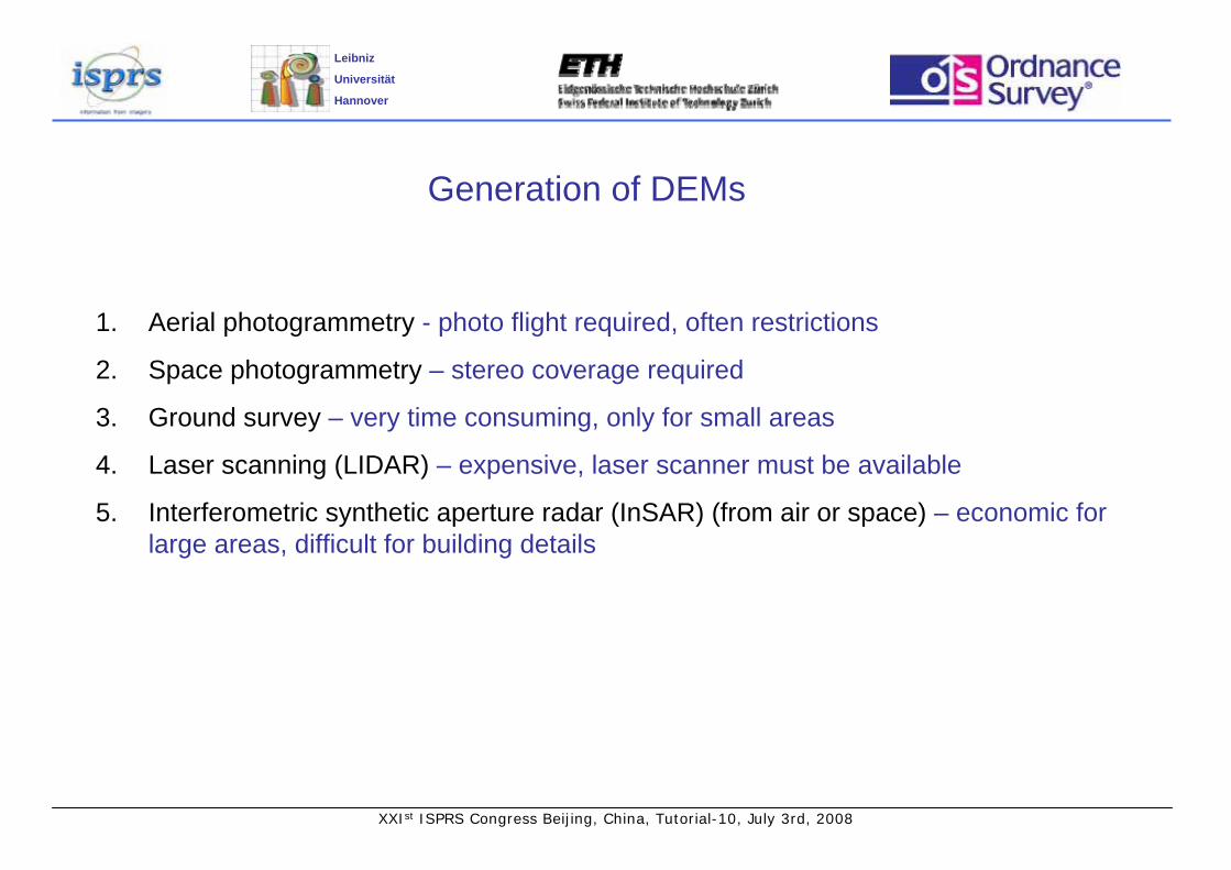
Generation of DEMs
1. Aerial photogrammetry - photo flight required, often restrictions
2. Space photogrammetry – stereo coverage required
3. Ground survey – very time consuming, only for small areas
4. Laser scanning (LIDAR) – expensive, laser scanner must be available
5. Interferometric synthetic aperture radar (InSAR) (from air or space) – economic for large areas, difficult for building details

XXIst ISPRS Congress Beijing, China, Tutorial-10, July 3rd, 2008
Leibniz
Universität
Hannover
Digital Elevation Models (DEM)
DEM representation of the bare ground by a grid of points – generalization by grid spacing one Z-value for every X-Y-point
XXIst ISPRS Congress Beijing, China, Tutorial-10, July 3rd, 2008
Leibniz
Universität
Hannover
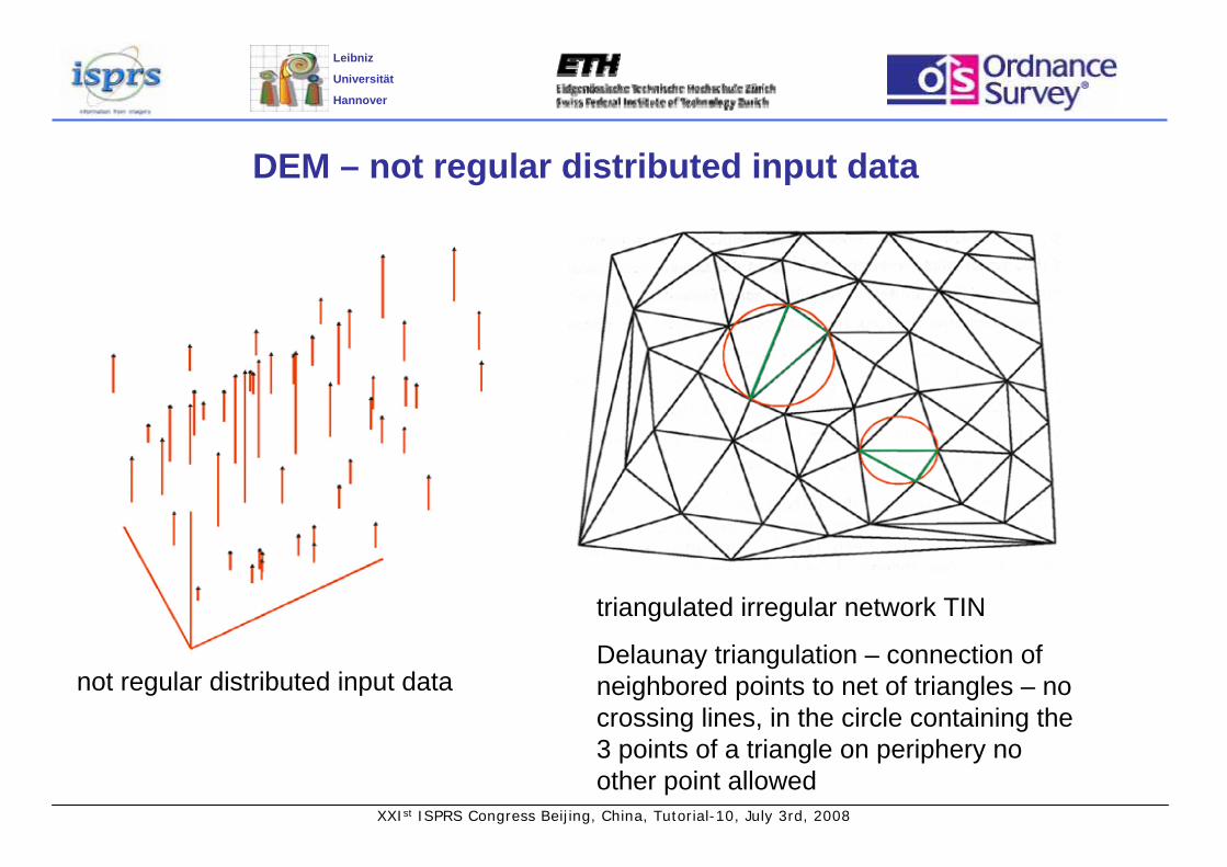
DEM – not regular distributed input data
not regular distributed input data
triangulated irregular network TIN
Delaunay triangulation – connection of neighbored points to net of triangles – no crossing lines, in the circle containing the 3 points of a triangle on periphery no other point allowed
XXIst ISPRS Congress Beijing, China, Tutorial-10, July 3rd, 2008
Leibniz
Universität
Hannover
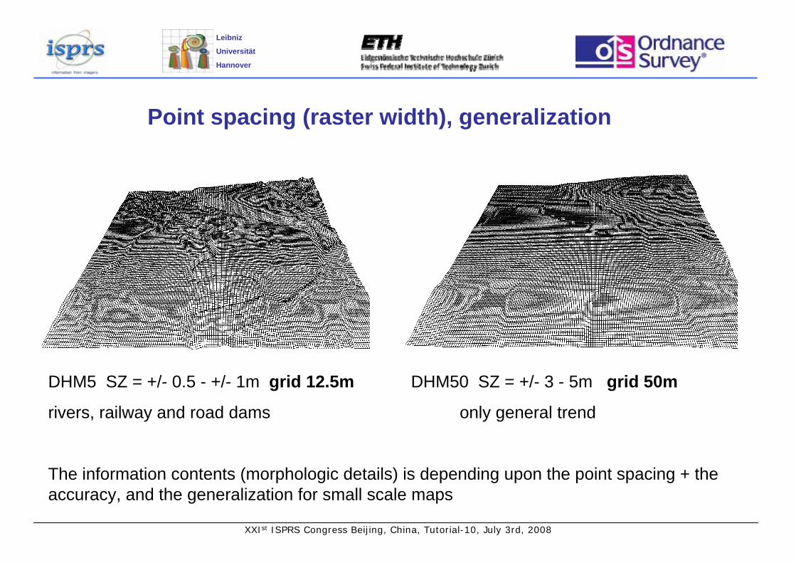
Point spacing (raster width), generalization
DHM5 SZ = +/- 0.5 - +/- 1m grid 12.5m DHM50 SZ = +/- 3 - 5m grid 50m
rivers, railway and road dams only general trend
The information contents (morphologic details) is depending upon the point spacing + the accuracy, and the generalization for small scale maps

XXIst ISPRS Congress Beijing, China, Tutorial-10, July 3rd, 2008
Leibniz
Universität
Hannover
height reference – mean sea level or geoid Geoid undulation
EGM96 geoid

XXIst ISPRS Congress Beijing, China, Tutorial-10, July 3rd, 2008
Leibniz
Universität
Hannover
Available SRTM C-band + X-band DEMfrom Shuttle Radar Topography Mission (SRTM) C-band InSAR DEMs covering 99.96% of land area from 56° south – 60.25° north available 0.15% gapsoutside USA spacing 3” (~90m), in USA 1” (~30m)
X-band data can be bought from German DLR with spacing 1“, but with large gaps between covered strips
SRTM C-band DEMs Arizona
10km x 10km
spacing 1“ spacing 3”
red: covered by X-band

XXIst ISPRS Congress Beijing, China, Tutorial-10, July 3rd, 2008
Leibniz
Universität
Hannover
SRTM height model Beijing
39°
40°
116° 117°
0m
987m

XXIst ISPRS Congress Beijing, China, Tutorial-10, July 3rd, 2008
Leibniz
Universität
Hannover
Tiles analysed are only the ones completely inland
problems in steep mountainous areas + dry sand dessert (low dielectric constant)
no reflection from water surface without waves
SRTM C-band - Global distribution of voids per 1º tileN20W010
Voids in sand dessert
Voids in mountainous area (Mt. Everest)

XXIst ISPRS Congress Beijing, China, Tutorial-10, July 3rd, 2008
Leibniz
Universität
Hannover
Z-accuracy as function of aspectsShuttle Radar Topography Mission (SRTM) - X-band DEM
RMSZ for:
terrain inclination 0.0
over all points
For average terrain inclination
Factor B ( RMSZ = A + B ∗ tan α )

XXIst ISPRS Congress Beijing, China, Tutorial-10, July 3rd, 2008
Leibniz
Universität
Hannover
Shuttle Radar Topography Mission (SRTM) C-band height model
If this accuracy and the 3 arcsec resolution cannot be accepted, DEMs have to be generated by other methods

XXIst ISPRS Congress Beijing, China, Tutorial-10, July 3rd, 2008
Leibniz
Universität
Hannover
Automatic image matching
Task: identification of corresponding points in 2 overlapping images for getting 3-D ground coordinates by intersection
Classic method: image correlation (area based)
Feature based matching (identification of clear objects like corners)
Least squares matching (area based, adjustment of corresponding sub-images)
Corresponding OrbView 3 sub-images h/b=1.4

XXIst ISPRS Congress Beijing, China, Tutorial-10, July 3rd, 2008
Leibniz
Universität
Hannover
Problems with matching in build up areas
orbit
first imagingsecond imaging
imaged area
base
left top top right
View shadow right view shadow left= points which can be determined
convergence angle
IKONOS Maras
h/b = 7.5
OrbView-3 Zonguldak h/b
= 1.4
heig
ht
SZ = GSD * h/b * factorfactor ~ 0.3 -1

XXIst ISPRS Congress Beijing, China, Tutorial-10, July 3rd, 2008
Leibniz
Universität
Hannover
automatic image matching – image correlation
Mustermatrix Suchmatrixpattern matrix search matrix
left image right imageproblem: approximate relation of both images – depending upon height variation
SrSlSlrr•
=
Area based matching

XXIst ISPRS Congress Beijing, China, Tutorial-10, July 3rd, 2008
Leibniz
Universität
Hannover
automatic image matching – epipolar information
Search matrix should have a limited size to reduce the computation time and to avoid problems of second maximum
Location of conjugate point in second image is depending upon terrain height
Approximate terrain height or conjugate position required
Usually the terrain height of one point is close to the neighboured – exception: vertical objects like buildings or cliffs
In any case problem of start point (first point for correlation requires some approximate location information)
epipolar line
Area based matching

XXIst ISPRS Congress Beijing, China, Tutorial-10, July 3rd, 2008
Leibniz
Universität
Hannover
Vertical line locus (VLL)Based on known orientation transformation of a square in object space with centre Xi, Yi and estimated height Zn into both images and computation of correlation coefficient, same with sequence of different Z-values
Z1
Z2
Z3
…
0
0,2
0,4
0,6
0,8
1 2 3 4 5 6 7 8 9 10 11 12 Zn
r
maximum of correlation coefficient = Z of terrainAdvantage: determined object points do have
exactly pre-defined the X-Y-location e.g. exact raster of points without interpolation
Image orientation requiredArea based matching

XXIst ISPRS Congress Beijing, China, Tutorial-10, July 3rd, 2008
Leibniz
Universität
Hannover
Image pyramids
One possibility to solve problem of approximate terrain height = use of image pyramids
Stepwise reduction of image, start matching in highest level of image pyramid rough DEM = start information for matching in pyramid level below, continuing up to lowest pyramid level

XXIst ISPRS Congress Beijing, China, Tutorial-10, July 3rd, 2008
Leibniz
Universität
Hannover
Region growing
Other method for solving problem with approximate image relation
Start with at least one conjugate point (seed point), matching all directly neighbored points, continuing with point having largest correlation coefficient, matching all neighbored points, which have not been matched before, continuing with point having largest correlation coefficient, . . .
No image orientation required, also for images with unknown geometry, disadvantage, seed points on islands required
Start at seed point

XXIst ISPRS Congress Beijing, China, Tutorial-10, July 3rd, 2008
Leibniz
Universität
Hannover
Feature based matchingidentification of features – e.g. corner points in both images, by image operators
image pyramidsreduction of original image step by step –identification of correspondence at highest level of pyramid – with smallest number of pixels –approximate relation of images improved step by step in next lower levels of pyramid

XXIst ISPRS Congress Beijing, China, Tutorial-10, July 3rd, 2008
Leibniz
Universität
Hannover
image correlation - problemseffect of relief to image correlation – image correlation is based on normal case + horizontal terrain
effect of steep terrain
same image scale
IRS-1C Himalayan

XXIst ISPRS Congress Beijing, China, Tutorial-10, July 3rd, 2008
Leibniz
Universität
Hannover
least squares matchingsimple image correlation based on horizontal ground elements
least squares matching
ybxbbyyaxaax′⋅+′⋅+=′′′⋅+′⋅+=′′
210
210
),(),( 10 yxgrryxg ′′′′′′⋅+=′′′highest possible accuracy of automatic image matching problem: limited range of convergence solution: at first image correlation
in open area more precise like human operator
result: Digital Surface Model (DSM)

XXIst ISPRS Congress Beijing, China, Tutorial-10, July 3rd, 2008
Leibniz
Universität
Hannover
Scale Invariant Feature Transform (SIFT)
smoothing Gaussian filter + image pyramid difference between images in adjacent levelsextreme values of the difference of the Gausian pyramid (DoG) computed on scale and space
are selected as key points
Example of key points corresponding to extreme values on a DoG pyramid
Very robust method, but not sub-pixel accuracy, can be used as seed points for least squares matching

XXIst ISPRS Congress Beijing, China, Tutorial-10, July 3rd, 2008
Leibniz
Universität
Hannover
Scale Invariant Feature Transform (SIFT)
Sub-image taken by IKONOS with high
buildings
Red: points determined by least squares adjustment with region growing – top of high buildings could not
be reached
Combined method: SIFT used for determination of seed points, followed by least squares adjustment
with region growing

XXIst ISPRS Congress Beijing, China, Tutorial-10, July 3rd, 2008
Leibniz
Universität
Hannover
effect of seasonal change to panchromatic SPOT images
June August
XXIst ISPRS Congress Beijing, China, Tutorial-10, July 3rd, 2008
Leibniz
Universität
Hannover
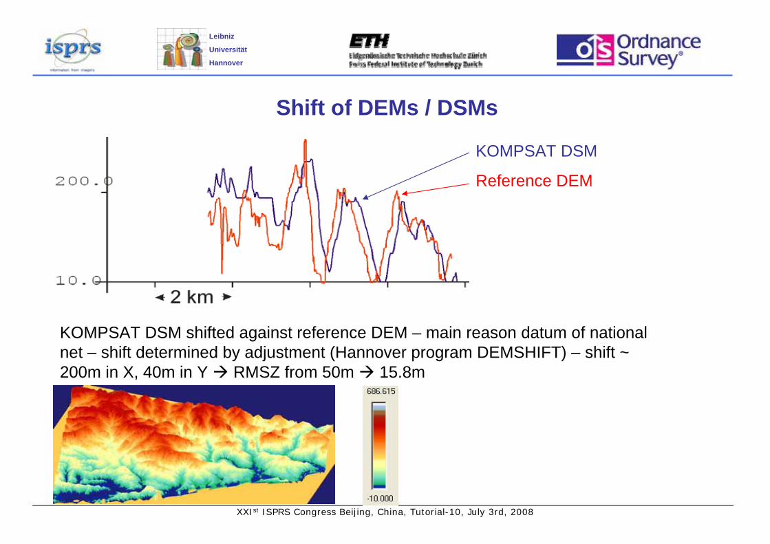
Shift of DEMs / DSMs
KOMPSAT DSM
Reference DEM
KOMPSAT DSM shifted against reference DEM – main reason datum of national net – shift determined by adjustment (Hannover program DEMSHIFT) – shift ~ 200m in X, 40m in Y RMSZ from 50m 15.8m

XXIst ISPRS Congress Beijing, China, Tutorial-10, July 3rd, 2008
Leibniz
Universität
Hannover
RMSZ as function of terrain inclination
0
5
10
15
20
25
30
.00
.10
.20
.30
.40
.50
.60
.70
.80
.90
1.00
For open areas:
RMSZ = 15.81m bias 0.72m
RMSZ = 13.0m + 10.9 * tan α
For all data dependency of vertical accuracy depending upon tan (slope)
In forest influence of vegetation – separate analysis in forest and open areas based on forest layer
Tangent terrain inclination
RMSZ [m]ASTER, 15m GSD, h/b = 1.7 (b/h=0.6)

XXIst ISPRS Congress Beijing, China, Tutorial-10, July 3rd, 2008
Leibniz
Universität
Hannover
DSM generation with KOMPSAT 1, Zonguldak
Quality map of image matching by least squares adjustment
Grey value 255 = correlation coeff. = 1.0Grey value 51 = correlation coeff. = 0.6
c < 0.6 = image as background
Black Sea
no overlap
> 0.95
< 0.90
< 0.80
< 0.70
< 0.60
< 0.50
< 0.40
< 0.30
< 0.20
< 0.10
< 0.00
Frequency distribution of correlation coefficients, acceptance limit = 0.6
No matching in water, poor results in dark forest
6.6m GSD height / base = 2.3 Spectral range: 0.51 – 0.73µm

XXIst ISPRS Congress Beijing, China, Tutorial-10, July 3rd, 2008
Leibniz
Universität
Hannover
Accuracy of KOMPSAT height model
0.912.2m + 12.7m ∗ tan α15.8mForest0.913.0m + 10.9m ∗ tan α15.8mOpen area
RMSpx [GSD]for flat terrain
RMSZ F(α)RMSZ
histogram of DZ for open area histogram of DZ for forest
KOMPSAT DEM above reference
Histogram with changed sign
2m bias
Histogram with changed sign
influence of forest
influence of buildings
XXIst ISPRS Congress Beijing, China, Tutorial-10, July 3rd, 2008
Leibniz
Universität
Hannover
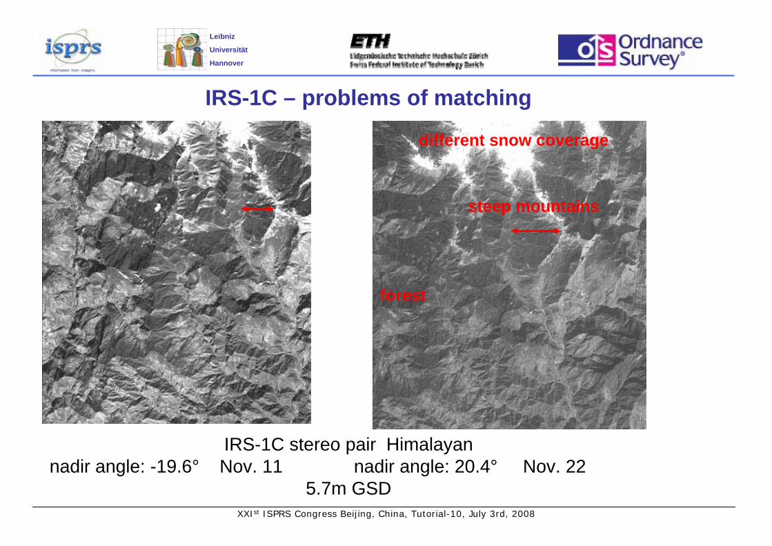
IRS-1C – problems of matching
IRS-1C stereo pair Himalayannadir angle: -19.6° Nov. 11 nadir angle: 20.4° Nov. 22
5.7m GSD
different snow coverage
steep mountains
forest

XXIst ISPRS Congress Beijing, China, Tutorial-10, July 3rd, 2008
Leibniz
Universität
Hannover
problems of automatic image matching (IRS-1C)
1. low contrast in forest
2. seasonal change of snow coverage
3. steep slopes

XXIst ISPRS Congress Beijing, China, Tutorial-10, July 3rd, 2008
Leibniz
Universität
Hannover
IRS-1C – DSM-generation
DEM based on IRS-1C height/base = 1.25
distribution of matched points774000 points = 1290 points/km²
40% matched
snow
forest steep slope
XXIst ISPRS Congress Beijing, China, Tutorial-10, July 3rd, 2008
Leibniz
Universität
Hannover
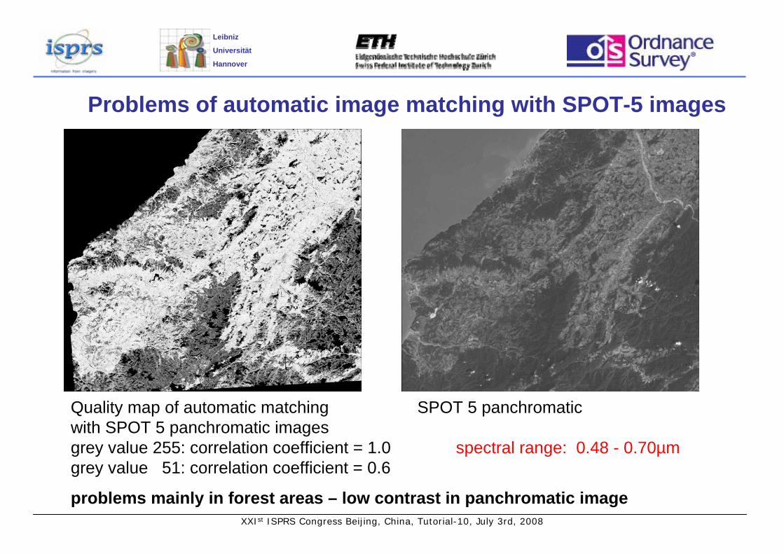
Problems of automatic image matching with SPOT-5 images
Quality map of automatic matching SPOT 5 panchromaticwith SPOT 5 panchromatic imagesgrey value 255: correlation coefficient = 1.0 spectral range: 0.48 - 0.70µmgrey value 51: correlation coefficient = 0.6
problems mainly in forest areas – low contrast in panchromatic image
XXIst ISPRS Congress Beijing, China, Tutorial-10, July 3rd, 2008
Leibniz
Universität
Hannover
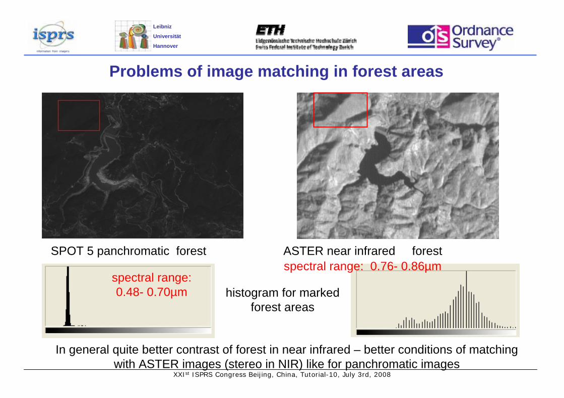
Problems of image matching in forest areas
SPOT 5 panchromatic forest ASTER near infrared forest
histogram for marked forest areas
In general quite better contrast of forest in near infrared – better conditions of matching with ASTER images (stereo in NIR) like for panchromatic images
spectral range: 0.48- 0.70µm
spectral range: 0.76- 0.86µm
XXIst ISPRS Congress Beijing, China, Tutorial-10, July 3rd, 2008
Leibniz
Universität
Hannover
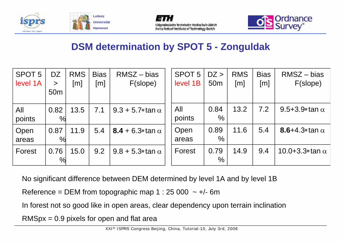
DSM determination by SPOT 5 - Zonguldak
9.8 + 5.3∗tan α9.215.00.76%
Forest
8.4 + 6.3∗tan α5.411.90.87%
Openareas
9.3 + 5.7∗tan α7.113.50.82%
All points
RMSZ – bias F(slope)
Bias[m]
RMS [m]
DZ >
50m
SPOT 5 level 1A
10.0+3.3∗tan α9.414.90.79%
Forest
8.6+4.3∗tan α5.411.60.89%
Open areas
9.5+3.9∗tan α7.213.20.84%
All points
RMSZ – bias F(slope)
Bias[m]
RMS [m]
DZ > 50m
SPOT 5 level 1B
No significant difference between DEM determined by level 1A and by level 1B
Reference = DEM from topographic map 1 : 25 000 ~ +/- 6m
In forest not so good like in open areas, clear dependency upon terrain inclination
RMSpx = 0.9 pixels for open and flat area
XXIst ISPRS Congress Beijing, China, Tutorial-10, July 3rd, 2008
Leibniz
Universität
Hannover
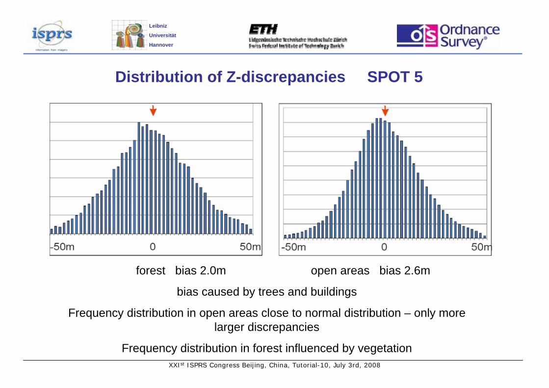
Distribution of Z-discrepancies SPOT 5
forest bias 2.0m open areas bias 2.6m
bias caused by trees and buildings
Frequency distribution in open areas close to normal distribution – only more larger discrepancies
Frequency distribution in forest influenced by vegetation

XXIst ISPRS Congress Beijing, China, Tutorial-10, July 3rd, 2008
Leibniz
Universität
Hannover
DSM generation with ASTER images
ASTER – Japanese sensor on Terra platformR, G, NIR with 15m GSD NIR nadir + backward 24° stereo in orbit
Intersection angle 27.2° - height to base relation = 2.0
Original sub-image after destriping (RADCOR)
Preparation of ASTER images -destriping

XXIst ISPRS Congress Beijing, China, Tutorial-10, July 3rd, 2008
Leibniz
Universität
Hannover
ASTER - DSM generation, Zonguldak, Turkey
Quality image 255 = c = 1.0 51 = c = 0.6
frequency distribution of correlation coefficients – most values > r=0.95
absolutely no problems with image matching – not matched points: mainly water, few small clouds - also good results in forest area (influence of near infrared band λ = 0.76µm – 0.86µm)
Bundle orientation with 42 control points from map 1 : 50 000 SX=SY=13m, SZ=11m
Quality map SPOT
XXIst ISPRS Congress Beijing, China, Tutorial-10, July 3rd, 2008
Leibniz
Universität
Hannover
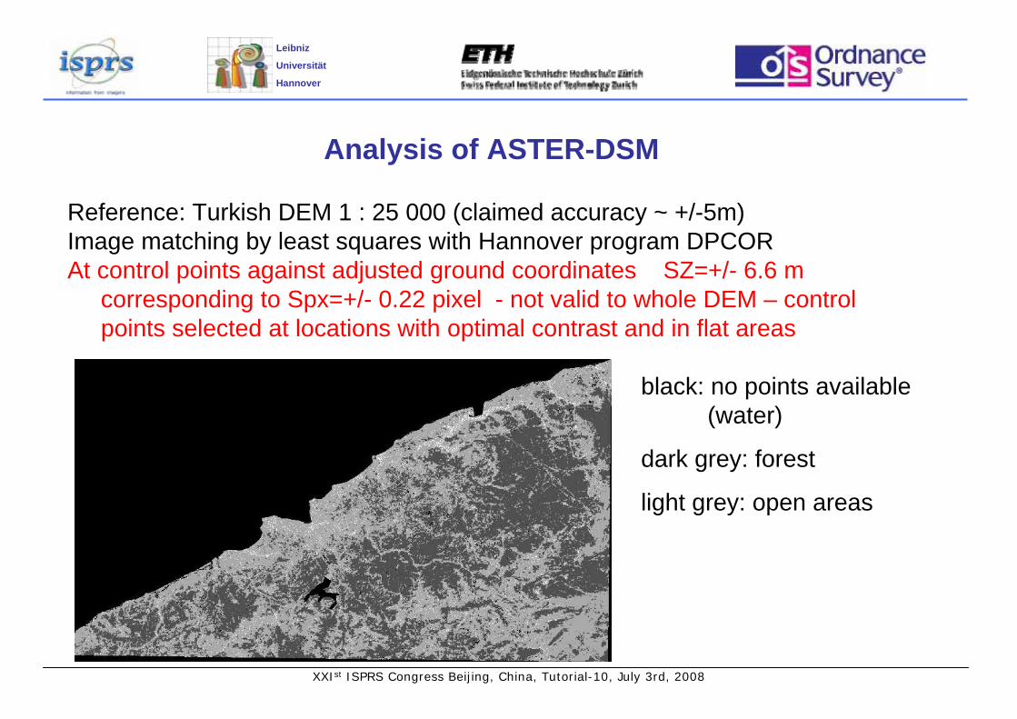
Analysis of ASTER-DSM
Reference: Turkish DEM 1 : 25 000 (claimed accuracy ~ +/-5m)Image matching by least squares with Hannover program DPCORAt control points against adjusted ground coordinates SZ=+/- 6.6 m
corresponding to Spx=+/- 0.22 pixel - not valid to whole DEM – control points selected at locations with optimal contrast and in flat areas
black: no points available (water)
dark grey: forest
light grey: open areas
XXIst ISPRS Congress Beijing, China, Tutorial-10, July 3rd, 2008
Leibniz
Universität
Hannover
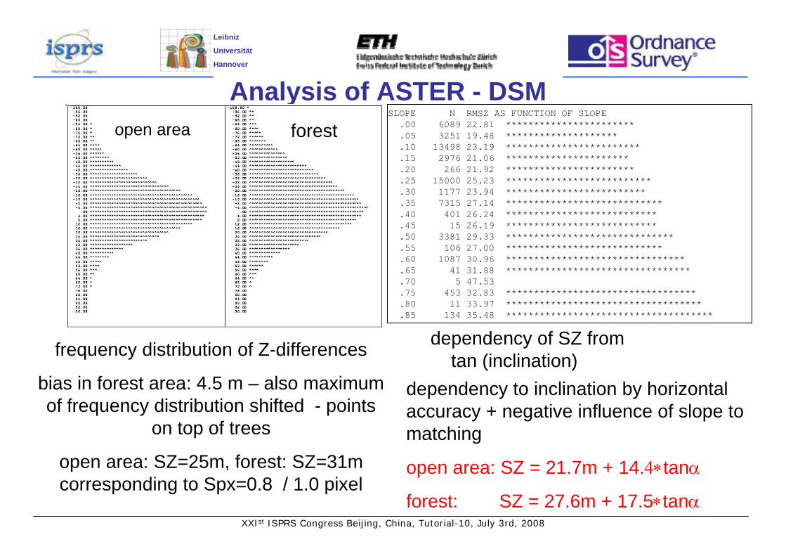
Analysis of ASTER - DSM
frequency distribution of Z-differences
bias in forest area: 4.5 m – also maximum of frequency distribution shifted - points
on top of trees
open area: SZ=25m, forest: SZ=31mcorresponding to Spx=0.8 / 1.0 pixel
forestopen areaSLOPE N RMSZ AS FUNCTION OF SLOPE .00 6089 22.81 *********************** .05 3251 19.48 ******************** .10 13498 23.19 ************************ .15 2976 21.06 ********************** .20 266 21.92 *********************** .25 15000 25.23 ************************** .30 1177 23.94 ************************* .35 7315 27.14 **************************** .40 401 26.24 *************************** .45 15 26.19 *************************** .50 3381 29.33 ****************************** .55 106 27.00 **************************** .60 1087 30.96 ******************************** .65 41 31.88 ********************************* .70 5 47.53 .75 453 32.83 ********************************** .80 11 33.97 *********************************** .85 134 35.48 *************************************
dependency of SZ from tan (inclination)
dependency to inclination by horizontal accuracy + negative influence of slope to matching
open area: SZ = 21.7m + 14.4∗tanα
forest: SZ = 27.6m + 17.5∗tanα

XXIst ISPRS Congress Beijing, China, Tutorial-10, July 3rd, 2008
Leibniz
Universität
Hannover
DSM generation with IKONOS Geo-images
dh
imag
e
reference plane
projection center
second image
position inleft scene
position inright scene
correct 3-D-position
orbit
first imagingsecond imaging
imaged area
height-baserelation7.5
automatic image matching with DPCOR
accuracy of building heights = 1.7m corresponding Spx=0.22m = 0.22 pixel
Dt = 12 sec
base=90km

XXIst ISPRS Congress Beijing, China, Tutorial-10, July 3rd, 2008
Leibniz
Universität
Hannover
Matching IKONOS, 1m pan h/b = 7.5
Least square matching 10 x 10 pixels, point spacing 3, no filter
noisy, some matching errors
10 x 10 pixels, point spacing 1, median filter 7 x 7
smooth results, vertical parts inclined in DSM

XXIst ISPRS Congress Beijing, China, Tutorial-10, July 3rd, 2008
Leibniz
Universität
Hannover
Problems of matching high resolution images in cities
forward viewbackward view
image in backward view
image in forward view
not visible in left / right image
Image of buildings different seen from left and right side, not visible parts, sudden change of x-parallax
sub-matrixes do not fit well –smaller problems with larger height/base-relation
top of buildingSide (vertical part) of building
base
heightheight
base
Large angle of convergence has disadvantage in build up areas

XXIst ISPRS Congress Beijing, China, Tutorial-10, July 3rd, 2008
Leibniz
Universität
Hannover
filtering of DSM DEM
matched pointssurface determined by simple mean value filter
simple filter will generate smooth surface, but not a DEM with points belonging to ground

XXIst ISPRS Congress Beijing, China, Tutorial-10, July 3rd, 2008
Leibniz
Universität
Hannover
Filtering DSM DEMforest
Identification and removal of points not belonging to bare ground
after filtering with Hannover program RASCOR

XXIst ISPRS Congress Beijing, China, Tutorial-10, July 3rd, 2008
Leibniz
Universität
Hannover
Filtering SRTM-DSM Bangkok
in Bangkok terrain height < 4m, SRTM-DSM includes Z-values up to 44mFiltering digital surface model (DSM) DEM –only successful if noise < influence of vegetation and buildings + available values on the bare groundIn Bangkok-DEM by filtering limitation of Zmax to 6.1m59% of points in city area removed by filtering
color coded DEMwithout after filteringZmax = 44m Zmax=6.1m
3D-view to original SRTM-DSM 1° elevation – similar to sky-line
3D-view to filtered SRTM-DEM 1° elevation

XXIst ISPRS Congress Beijing, China, Tutorial-10, July 3rd, 2008
Leibniz
Universität
Hannover
Filtering DSM DEMgrey value coded DSM determined by automatic matching
- buildings can be recognized
matched DSM
filtered DEM (RASCOR)

XXIst ISPRS Congress Beijing, China, Tutorial-10, July 3rd, 2008
Leibniz
Universität
Hannover
Effect of filtering to generated contour lines
contour interval: 4 ft
left: original data set from image matching
right: after filtering

XXIst ISPRS Congress Beijing, China, Tutorial-10, July 3rd, 2008
Leibniz
Universität
Hannover
Cartosat-1
Launched May 2005
2 optics 26° ahead, 5° behind stereo in orbit
Δt for nadir orientation 58 sec
distance to base relation 1.44
Flexible orientation – rotation to side possible
In case of nadir orientation: GSD ahead:~ 2.5m x 2.5mGSD behind:~ 2.2m x 2.5m
swath: 12 000 pixels - 30 km
Configuration Istiranca8.8° roll

XXIst ISPRS Congress Beijing, China, Tutorial-10, July 3rd, 2008
Leibniz
Universität
Hannover
Automatic image matching of Cartosat stereo model
matched points overlaid to image white = matched pointsgaps mainly caused by clouds
quality image: grey value corresponds to correlation coefficient r=1.0 = white
r=0.5 = grey value 123
Automatic image matching by least squares – excellent results for mountainous forest

XXIst ISPRS Congress Beijing, China, Tutorial-10, July 3rd, 2008
Leibniz
Universität
Hannover
Automatic image matching of Cartosat stereo model
0 20000 40000 60000 80000
0.95
0.85
0.70
0.55
0.40
0.25
0.10
Frequency distribution of correlation coefficientsTolerance limit = 0.5Cartosat-1 spectral range from 0.50 up to 0.85µm – including near infrared = good contrast also in forest
Histogram SPOT-5 HRSspectral range0.48- 0.70µmonly forest
Histogram Cartosat in forest area Forest area in
Cartosat-1
XXIst ISPRS Congress Beijing, China, Tutorial-10, July 3rd, 2008
Leibniz
Universität
Hannover
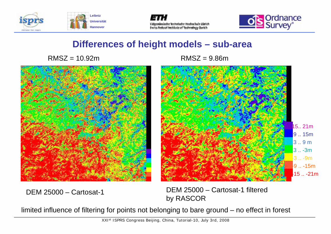
Differences of height models – sub-area
DEM 25000 – Cartosat-1 DEM 25000 – Cartosat-1 filtered by RASCOR
15.. 21m9 .. 15m3 .. 9 m3 .. -3m
-3 .. -9m-9 .. -15m-15 .. -21m
limited influence of filtering for points not belonging to bare ground – no effect in forest
RMSZ = 10.92m RMSZ = 9.86m
XXIst ISPRS Congress Beijing, China, Tutorial-10, July 3rd, 2008
Leibniz
Universität
Hannover
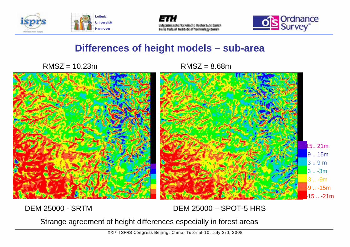
Differences of height models – sub-area
DEM 25000 - SRTM DEM 25000 – SPOT-5 HRS
15.. 21m9 .. 15m3 .. 9 m3 .. -3m
-3 .. -9m-9 .. -15m-15 .. -21m
RMSZ = 10.23m RMSZ = 8.68m
Strange agreement of height differences especially in forest areas
XXIst ISPRS Congress Beijing, China, Tutorial-10, July 3rd, 2008
Leibniz
Universität
Hannover
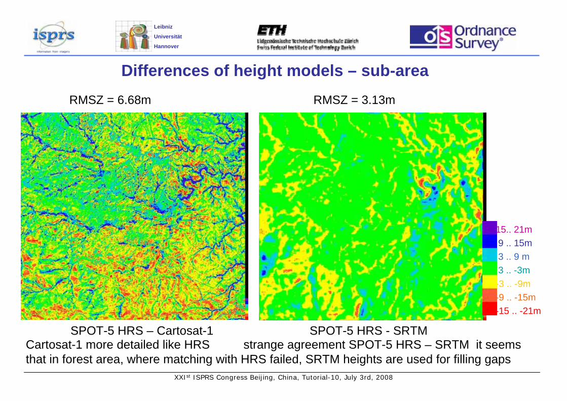
Differences of height models – sub-area
SPOT-5 HRS – Cartosat-1 SPOT-5 HRS - SRTM
RMSZ = 6.68m RMSZ = 3.13m
Cartosat-1 more detailed like HRS strange agreement SPOT-5 HRS – SRTM it seems that in forest area, where matching with HRS failed, SRTM heights are used for filling gaps
15.. 21m9 .. 15m3 .. 9 m3 .. -3m
-3 .. -9m-9 .. -15m-15 .. -21m

XXIst ISPRS Congress Beijing, China, Tutorial-10, July 3rd, 2008
Leibniz
Universität
Hannover
Influence of DEM interpolation
15.. 21m9 .. 15m3 .. 9 m3 .. -3m
-3 .. -9m-9 .. -15m-15 .. -21m
SPOT-5 HRS – Cartosat-1point spacing Cartosat-1 7.5m
HRS height model reduced from 20m spacing to 80m spacing and interpolated from 80m spacing to 20m again – resulting in such differences
Most effects HRS – Cartosat can be explained just by the different spacing – the reduction of HRS to 80m results in similar effects like difference HRS-Cartosat, it seems, the gaps of HRS have been filled with SRTM 1‘‘ spacing

XXIst ISPRS Congress Beijing, China, Tutorial-10, July 3rd, 2008
Leibniz
Universität
Hannover
Morphologic details
SRTM C-band 92m spacing SPOT-5 HRS 20m spacing
Cartosat-1 7.5m spacing DEM 25 000Also morphologic details of HRS are similar to SRTM – quite better for Cartosat-1

XXIst ISPRS Congress Beijing, China, Tutorial-10, July 3rd, 2008
Leibniz
Universität
Hannover
Colour coded Cartosat-1 height model in urban area
Amman

XXIst ISPRS Congress Beijing, China, Tutorial-10, July 3rd, 2008
Leibniz
Universität
Hannover
Accuracy of Cartosat-1 DSMs/DEMs checked against precise reference
2.93 + 1.81*tan a1.493.47Forest, filtered3.17 + 3.14*tan a0.483.30Open areas, filtered3.33 + 0.33*tan a0.923.55Forest3.91 + 1.64*tan a-0.514.02Open areasSZ as F(slope)biasSZ
3.11 + 6.50*tan a0.813.13Forest, filtered
2.39 + 8.80*tan a0.442.43Open areas, filtered
4.11 + 0.34*tan a0.644.37Forest
3.16 + 1.19*tan a-0.543.23Open areas
SZ as F(slope)biasSZ
2.69 + 1.97*tan a1.433.42Forest, filtered3.22 + 1.97*tan a-0.583.39Open areas, filtered2.82 + 1.70*tan a0.583.59Forest3.96 + 3.06*tan a-1.164.13Open areasSZ as F(slope)biasSZ
Mausanne, January
Mausanne, February
Warsaw

XXIst ISPRS Congress Beijing, China, Tutorial-10, July 3rd, 2008
Leibniz
Universität
Hannover
Morphologic quality of height models – contour lines
SRTM C-band 70/92m SRTM X-band 23/31m ASTER 45m
KOMPSAT-1 20m SPOT 5 15m map 1 : 25 000
contour interval 20m source with used point spacing
XXIst ISPRS Congress Beijing, China, Tutorial-10, July 3rd, 2008
Leibniz
Universität
Hannover
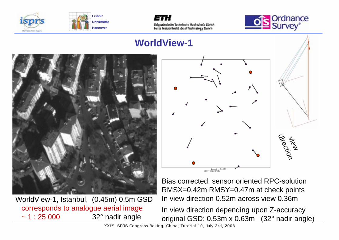
WorldView-1
WorldView-1, Istanbul, (0.45m) 0.5m GSDcorresponds to analogue aerial image ~ 1 : 25 000 32° nadir angle
Bias corrected, sensor oriented RPC-solutionRMSX=0.42m RMSY=0.47m at check pointsIn view direction 0.52m across view 0.36mIn view direction depending upon Z-accuracyoriginal GSD: 0.53m x 0.63m (32° nadir angle)
view
direction
XXIst ISPRS Congress Beijing, China, Tutorial-10, July 3rd, 2008
Leibniz
Universität
Hannover
Synthetic Aperture Radar (SAR)
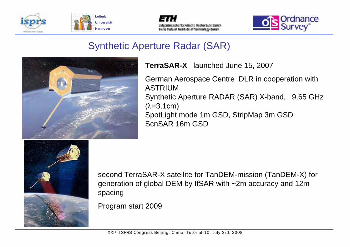
TerraSAR-X launched June 15, 2007
German Aerospace Centre DLR in cooperation with ASTRIUMSynthetic Aperture RADAR (SAR) X-band, 9.65 GHz (λ=3.1cm)SpotLight mode 1m GSD, StripMap 3m GSDScnSAR 16m GSD
second TerraSAR-X satellite for TanDEM-mission (TanDEM-X) for generation of global DEM by IfSAR with ~2m accuracy and 12m spacing
Program start 2009
XXIst ISPRS Congress Beijing, China, Tutorial-10, July 3rd, 2008
Leibniz
Universität
Hannover
ConclusionHeight models can be determined by automatic image matching of optical space images
DSMs are generated, for getting a DEM filtering required
Accuracy in forest not so good like in open areas – dependency upon spectral range
Especially in forest areas spectral range extended to NIR required
Accuracy as F(terrain inclination)
Accuracy at check points not identical to DEM accuracy
In general accuracy SZ = GSD * h/b * factor 0.2 < factor < 1.0
Morphologic details depending upon point spacing of DEM
Point spacing usually ~ 3 * GSD – only in special cases 1* GSD justified
With Cartosat-1 in open and flat terrain up to SZDEM= 2.4m
In future improved ground resolution + height models from TanDEM-X (expected: SZ=2m)
With very high resolution images (<0.5m GSD) similar condition like with aerial images