tutorial 3g.06 dewatering in a slope - cesar-lcpc

Tutorial 3g.06

Dewatering in a slope

Ref: CESAR-TUT(3g.06)-v2021.0.1-EN

CESAR - Tutorial 3g.06 1

1. INTRODUCTION

1.1. Tutorial objectives

Excess water infiltration came from rainfall may be a major cause of slope failure due to the rising of pore water pressure and the decrease in shear strength of the slope. It is then crucial to protect the slope in a way to discharge the ground water and to maintain the water pressure.

This tutorial aims to study the influence of subsurface drainage system in ground water flow. Two models will be compared: one without any drainage system and another with subsurface drainage system. After the hydraulic analysis, the study can be further conducted to hydro-mechanical analysis in order to observe the evolution of mechanical stress due to change in hydrostatic pressure.

This tutorial allows the user to learn:

✓ How to create a 3D volume from 2D geometry,

✓ How to obtain ground table water position and flow network in 3D model,

✓ How to conduct an uncoupled hydro-mechanical analysis with CESAR-LCPC.

1.2. Problems description

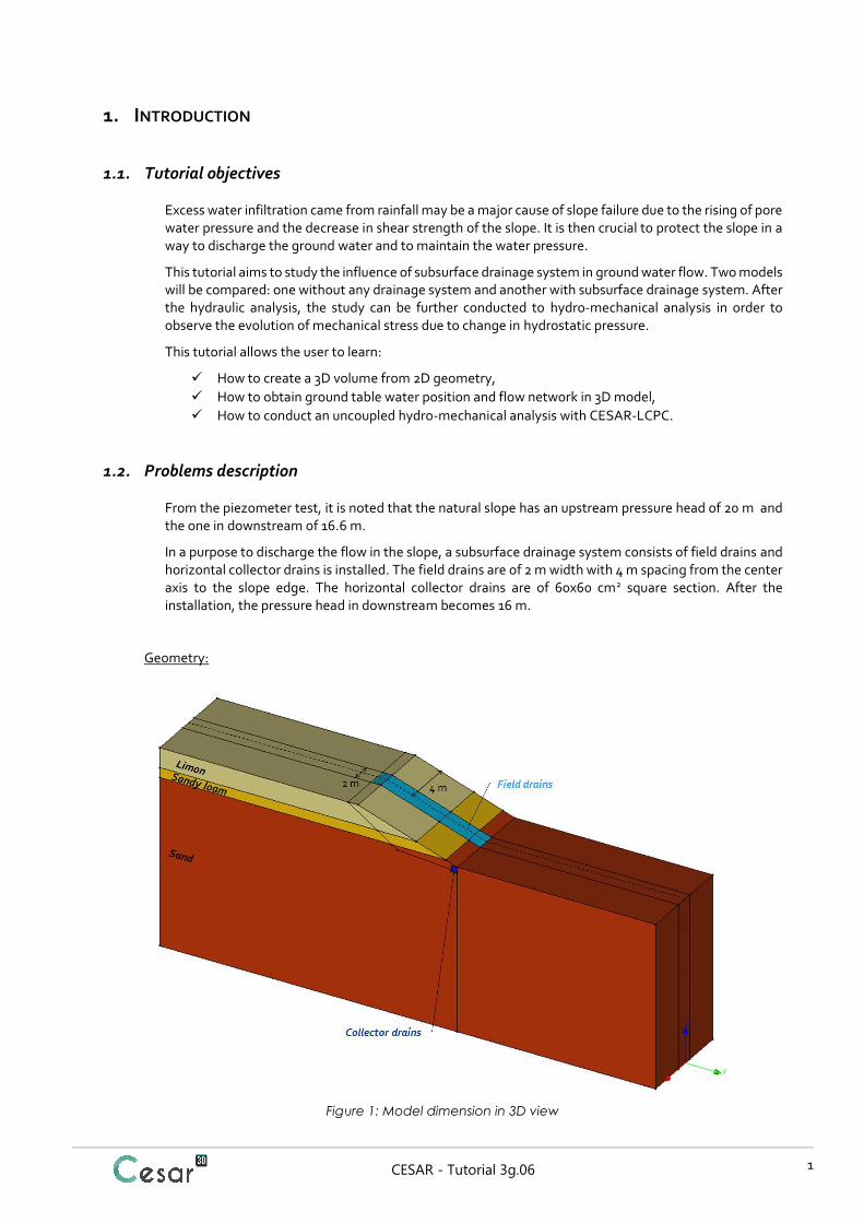
From the piezometer test, it is noted that the natural slope has an upstream pressure head of 20 m and the one in downstream of 16.6 m.

In a purpose to discharge the flow in the slope, a subsurface drainage system consists of field drains and horizontal collector drains is installed. The field drains are of 2 m width with 4 m spacing from the center axis to the slope edge. The horizontal collector drains are of 60x60 cm2 square section. After the installation, the pressure head in downstream becomes 16 m.

Geometry:

Figure 1: Model dimension in 3D view


Figure 2: Model dimension in OZY plan

Analysis stages:

Hydrogeological analysis

1. Initialisation of flow network – Natural slope

2. Initialisation of flow network – Slope with subsurface drainage

Mechanical analysis

3. Hydro-mechanical analysis – Natural slope

4. Hydro-mechanical analysis – Slope with subsurface drainage


2. GEOMETRY AND MESH

2.1. Geometry

Working plane settings:

1. Go to the tab GEOMETRY tab

2. Click on Tools:

- Set OZY as coordinates system plane.

- Set the visible grid to 0.2 m (dX = dY = dZ = 0.2m)

Drawing of the geometry:

1. Click on . The point definition dialog is displayed.

- Define the coordinates of the construction points (see Figure 1).

2. Use Lines to link the points previously defined.

3. Click on Edge partitions to divide the contour lines in the slope/field drains segments (between the segments 1-2-3-4-6).

Generation of the surfaces

After having the contour, we can now define the associated surface.

1. Activate Plane Surface.

2. Select all previously defined edges.

3. Apply.

Generation of the volumes

The volume of the slope is constructed using an extrusion of the plane surfaces.

1. On the Selections toolbar, activate only Select faces option.

2. Select all the surfaces to be extruded

3. Click on Extrusion and set:

- Translation as operation type,

- Generation of volume bodies as extrusion type,

- 1 as number of operations,

- (-3 ; 0 ; 0) as vector,

- Tick the box “Remove surface bodies”.

4. Apply

5. Repeat the procedure to complete the global volume

- 2nd extrusion operation with (-2 ; 0 ; 0) as vector

- 3rd extrusion operation with (-3 ; 0 ; 0) as vector


View of the model before last extrusion ("show" option)

Dissociation of bodies:

During extrusion operation, the initial faces selection is a group of 8 surfaces. However, the result of extrusion is one single body made of the association of 8 volume bodies. In order to distinguish the bodies with different material properties, it is necessary to split them.

1. Activate Explode bodies. Select a volume body. Apply.

2. Repeat the operation for the other extruded bodies.

Merge bodies and bodies edition:

This step is optional but it facilitates the assignment of material properties and loading case for a group of elements during multiple analysis stages.

1. On the Selection Toolbar, activate only Select bodies option.

2. Merge bodies operation:

- Activate Merge bodies,

- Select the volume bodies associated to “Field drains” (see Figure 1),

- Apply,

- Repeat the operation in order to group the other bodies associated to “Collector

drains”, “Limon”, “Sandy loam”, and “Sand” (see Figure 1).

3. Bodies edition:

- Activate Body properties.

- Right-click on the body corresponding to the “Field drains”. Specify a name and a

colour for this body. Click on Apply.

- Repeat previous operation for the other bodies.


2.2. Mesh

Mesh density definition :

1. Go to the MESH tab on the project flow bar.

2. Select Front view option to display the model in OZY plan.

3. Select all edges of the “Field drains” bodies. Click on Fixed length density to divide the segment with a fixed length. Enter 0.5 m in the dialog box. Click on Apply.

4. Select all edges of the “Collector drains” bodies. Click on Fixed length density to divide the segment with a fixed length. Enter 0.3 m in the dialog box. Click on Apply.

5. Click Variable density to propagate from the previous area to the model limits:

- Tick First / Last interval to define the method,

- Enter 0.5 m as First division and 5 m as Last division,

- Click on the lines which link the drainage system and the soil edges in order to

affect this density.

6. Select all the soil edges. Click on Fixed length density to divide the segment with a fixed length. Enter 5 m in the dialog box. Click on Apply.

7. Select Isoparametric view option to display the model in 3D plan.

8. Select the transversal line corresponding to the top of the slope:

- Click on Fixed length density,

- Enter 1 m in the dialog box,

- Tick “Propagate density to opposite sides,

- Click on Apply.

Volume meshing generation:

1. Select all the volume bodies.

2. Open the tool Volume meshing

- Select “Quadratic interpolation” as Interpolation type.

- Set “Regular mesh” as Mesh type.

- Apply.


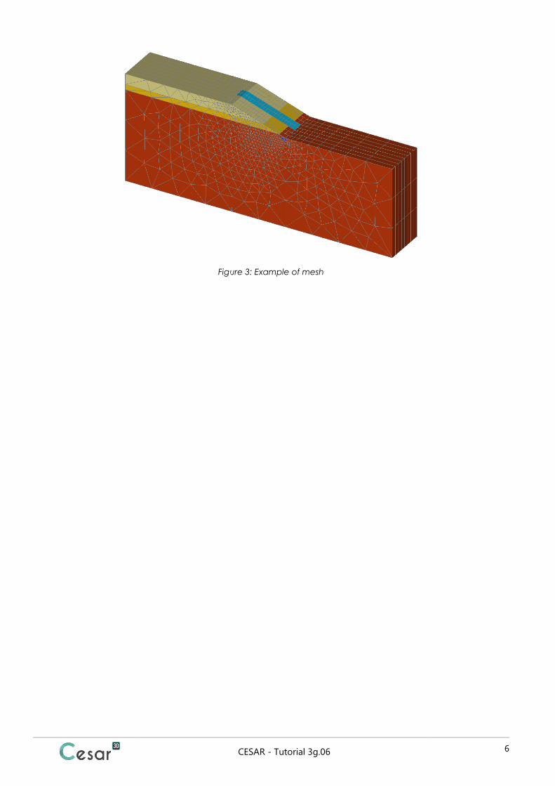
Figure 3: Example of mesh


3. HYDROGEOLOGICAL ANALYSIS

For analyzing the ground water flow in porous media with a potential unsaturated area, CESAR-LCPC provides NSAT module.

3.1. Natural slope

Model definition:

1. Right click on GROUNDWATER FLOW in the Study tree view on the right side of the working window.

2. Click on Add a model.

3. A new toolbox is open for definition of the Model:

- Enter Hydro-Natural as “Model name”,

- Select NSAT as “Solver”,

- Tick Initial parameters as calculation type,

- Click on Validate.

Material properties for the volume bodies:

It will be convenient to define all the material properties in the material library of the study before assigning to a body.

1. Go to the PROPERTIES tab.

2. Click on Properties for volume bodies.

3. Give a name for the properties set name (Limon for example).

- In Flow parameters, choose “Van Genuchten & Gardner” as unsaturated law,

- Set the parameter values as defined in the table below.

4. Click on to create another properties set.

5. Modify the name for the properties set (Sandy loam for example).

- In Flow parameters, choose “Van Genuchten & Gardner” as unsaturated law,

- Set the parameter values as defined in the table below.

6. Repeat the operation until all material properties are set.

7. Click on Validate and Close.

Limon

Sandy loam

Sand Field drains Collector drains

Saturated permeability coefficient

kxs, kys, kzs 1.10-4 5.10-5 3.10-4 1.10-2 1.10-1

kxy, kyz, kzx 0. 0. 0. 0. 0.

Unsaturated water content function1

s 0.40 0.36 0.35 0.5 0.5

r 0.10 0.28 0.12 0.01 0.01

0.20 0.34 0.22 0.05 0.05

n 1.8 1.60 1.50 2.0 2.0

m 0.44 0.38 0.33 0.5 0.5

Unsaturated permeability function2

a 0.02 0.03 0.04 0.01 0.01

nn 1.5 1.9 2.2 3.0 3.0


The constant parameters for the van Genuchten water content function and the Gardner permeability function are chosen based on literature study. User can also define these parameters manually by curve-fitting parameters from the results of laboratory experimental test. For more information, please refer to CESAR Manual Theory.

Reference pressure is the atmospheric pressure equals to 100 kPa.

Figure 4: Permeability function in NSAT module

Assignment of properties sets:

In this stage of analysis, the subsurface drainage system hasn’t yet installed. Hence, it is considered that the bodies corresponding to the subsurface drainage system have the natural soil properties.

1. Activate Assign properties tool.


3. Select all volume bodies corresponding to the surface bodies no 1-2 (refer to Figure 2)

- Select “Limon” properties set in the list.

- Apply.


- Select “Loam” properties set in the list.

- Apply.


- Select “Sand” properties set in the list.

- Apply.

Boundary conditions:

By default, the boundary condition will be named BCSet1. User can edit the name of boundary condition by pressing the [F2] key.

1. Go to the BOUNDARY CONDITIONS tab.



3. Click on Prescribed constant load.

- Select the surface bodies in upstream side. Enter 20 m as load value. Apply.

- Select the surface bodies in downstream side including the top surface of the

collector drain. Enter 16.6 m as load value. Apply.

4. Click on Seepage condition. Select the surface bodies of the top of the slope and along the slope. Apply.

Figure 5: Boundary condition in the natural slope

Analysis settings:

1. Go to the tab ANALYSIS then activate the Analysis settings .

2. In the Time steps section, choose “Steady state”.

3. In the Solution method section:

- Select “Fixed point method”

- Max number of iterations: 100

- Tolerance: 0,001

4. In the Storage for subsequent calculation section:

- Activate “Storage for subsequent calculation”

- Specify the folder path and the name of the file where the calculated hydraulic

pressure will be stored (extension *.rst).

5. Validate.


3.2. Slope with subsurface drainage system

Model definition:

1. In the data tree, right click on the previous model title and then select Copy of the model.

2. A toolbox is displayed for definition of this new model.

- Change the model name: Hydro-Drainage.

- Select “Initial parameters” as the type of calculation.

- Validate to close the toolbox for model definition.

3. A toolbox is displayed for setting the sharing options. By default, all the setting of the previous model is copied to the new model.

- Untick “Properties” and “Boundary conditions”,

- Let the default check mark in “Loadings”.

- Click on Validate.


Here the subsurface drainage system is installed. We have to modify the material properties to the properties of subsurface drainage system.

1. Select Isoparametric view option to display the model in 3D plan.

2. Activate Assign properties tool.


4. Select the volume bodies corresponding to the “Field drains” (refer to Figure 1)

- Select “Field drains” properties set in the list.

- Apply.

5. Repeat the operation to assign the properties of “Collector drains”.


By default, the boundary condition of the previous model is copied to the actual model. In this case, we only have to modify the pressure head in the downstream.

1. Go to the BOUNDARY CONDITIONS tab.


3. Click on Prescribed constant load.

- Select the surface bodies in downstream side including the top surface of the

collector drain. Enter 16 m as load value. Apply.

Analysis settings:

1. Go to the tab ANALYSIS then activate the Analysis settings .

2. No changes in Time steps and Solution method.

3. In the Storage for subsequent calculation section:

- Activate “Storage for subsequent calculation”

- Specify the folder path and the name of the file where the calculated hydraulic

pressure with subsurface drainage system will be stored (extension *.rst).

4. Validate.


4. RESULTS AND ANALYSIS

4.1. Flow network contour

We will compare the flow network in both models in order to see the influence of subsurface drainage system on the slope.

1. Go to tab RESULTS.

2. Click on Type of results to display.

- Select Undeformed as Mesh,

- Tick the box “Active” and select Water head in Contour plots section,

- Apply.

3. Click on Mesh settings.

- Select Group border as Mesh border,

- Apply.

4. Click on Contour plot settings.

- Tick the box “Activate” and select Areas as plot style,

- Tick the box “Contour lines” and select Grey as Color set,

- Select Manual as Scale and put 16. as manual inferior value and 20. as manual

superior value,

- Select Groundwater as Color scheme.

- Apply.

5. Click on Legend.

- Select Contour plot as Legend type,

- Tick the box “Legend border”,

- Apply.

Figure 6: Water head contour in natural slope condition


Figure 7: Water head contour in the slope with subsurface drainage system

4.2. Water table on the slope

For a better comparison analysis, we will compare the values of water head in the centre axis of the slope.

1. Go to tab CHARTS.

2. Activate Points on the Entities for charts toolbar.

- Create 3 points (A, B and C) to draw the line of centre axis.

3. Activate Lines on the Entities for charts toolbar.

- Click on two edges then double click until a red line appears.

4. Activate Line Set on the Entities for charts toolbar.

- Click on the two lines on the centre axis of the slope,

- Enter a name (for example “Axis”) in the Line set window,

- Click on Add.

5. Activate Charts for a line Set on the Charts toolbar.

- Select “Water head” as Parameter,

- Select the cut line of centre axis as Line set,

- Select the time step

- Click on Apply.


Figure 8: Cut line in the centre axis of the slope

(a) (b)

Figure 9: Comparison of water head values (a) Natural slope (b) Slope with subsurface drainage system

Figure 9 shows clearly the aquifer drawdown phenomenon due to the installation of subsurface drainage system. The water table on the top of the slope (at the upstream side) has progressively lowered about 0.3 to 1.6 m. The drainage system allows intercepting the aquifer. It can be seen also in Figures 7-8 that the aquifer drawdown occurs in the transversal plane of the slope.

A

B

C


5. FURTHER ANALYSIS: HYDRO-MECHANICAL ANALYSIS

After analysing the dewatering on the slope, a further analysis can be conducted in order to examine the mechanical stability of the slope. In this case study, an uncoupled analysis is chosen. The calculated hydraulic pressure resulting from the NSAT module will be used as a loading pressure condition for the MCNL module.

Model definition:

1. Right click on STATICS in the Study tree view on the right side of the working window.

2. Click on Add a model.

- Change the model name: Mech-Natural,

- Select “MCNL” as Solver,

- Select “Initial parameters” as the type of calculation,

- Validate to close the toolbox for model definition.

Material properties:

Follow the same procedure to register the material database.

1. Go to the tab PROPERTIES.

2. Activate Properties for volume bodies.

3. Click on to create another properties set.

4. Modify the name for the properties set, Limon for example.

- In Elasticity parameters, choose “Isotropic linear elasticity”. Set the values of , E

and as specified in the table below.

- In Plasticity parameters, choose “Drucker-Prager without hardening” as criterion.

Set the values of c, and as specified in the table below.

5. Click on Validate and Close.

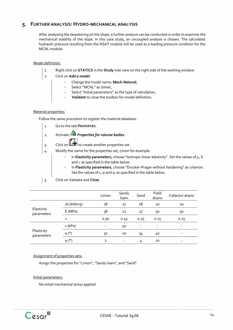
Limon Sandy loam

Sand Field

drains Collector drains

Elasticity parameters

h (kN/m3) 18 17 18 20 20

E (MPa) 38 22 27 50 50

0.30 0.45 0.25 0.25 0.25

Plasticity parameters

c (kPa) - 50 - - -

(°) 32 20 34 40 -

(°) 2 - 4 10 -


Assign the properties for “Limon”, “Sandy loam”, and “Sand”.

Initial parameters:

No initial mechanical stress applied.



1. Go the BOUNDARY CONDITIONS tab.

2. On the toolbar, activate to define side and bottom supports.

3. Apply. Supports are automatically affected to the limits of the mesh.

Loading set:

Default name of the boundary condition, LoadSet1, set can be edited using the [F2] key.

There will be two types of loading: one of gravitational force and another of calculated hydraulic pressure resulting from NSAT module.

1. Go to the LOADS tab.

2. On the toolbar, click on Gravity forces. Select all the bodies. Click on Apply.

3. On the toolbar, click on WTB-Isotropic pressure.

- On the Initial hydrostatic field, select “File” as Water head input.

- Specify the storage file of the calculated hydraulic pressure from the groundwater

analysis Hydro-Natural.

- Validate.

4. On the toolbar, activate WTB – unit weights.

- Unit weight: 0.019 MN/m3 (20 kN/m3)

- Saturated unit weight: 0.020 MN/m3 (20 kN/m3)

- Validate.

Analysis settings:

1. Go to the ANALYSIS tab, then activate Analysis settings .

2. In the General parameter section, enter the following values:

- Iteration process:

Max number of increments: 1

Max number of iterations per increment: 500

Tolerance: 0,001

- Method of resolution: 1- initial stresses

- Solver type: Multifrontal

3. Validate.

Edited by :

8 quai Bir Hakeim

F-94410 SAINT-MAURICE

Tél. : +33 1 49 76 12 59

[email protected]

www.cesar-lcpc.com

© itech - 2020

tutorial 3g.06 dewatering in a slope - cesar-lcpc

Documents