tutorial examine 2d

Quick Start Tutorial 1-1

Quick Start Tutorial

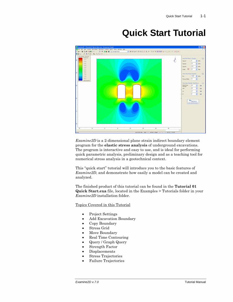
Examine2D is a 2-dimensional plane strain indirect boundary element program for the elastic stress analysis of underground excavations. The program is interactive and easy to use, and is ideal for performing quick parametric analysis, preliminary design and as a teaching tool for numerical stress analysis in a geotechnical context.

This “quick start” tutorial will introduce you to the basic features of Examine2D, and demonstrate how easily a model can be created and analyzed.

The finished product of this tutorial can be found in the Tutorial 01 Quick Start.exa file, located in the Examples > Tutorials folder in your Examine2D installation folder.

Topics Covered in this Tutorial

• Project Settings • Add Excavation Boundary • Copy Boundary • Stress Grid • Move Boundary • Real Time Contouring • Query / Graph Query • Strength Factor • Displacements • Stress Trajectories • Failure Trajectories

Examine2D v.7.0 Tutorial Manual


Introduction

Before launching into an analysis with Examine2D, it is important to stop and consider the developmental philosophy of the program, the assumptions inherent in the analysis and the resultant limitations.

Examine2D is designed to be a quick and simple-to-use parametric analysis tool for investigating the influence of geometry and in-situ stress variability on the stress changes in rock due to excavations. The induced stresses in the plane of the analysis can be viewed by means of stress contour patterns in the region surrounding the excavations. As a tool for interpreting the amount of deviatoric overstress (principal stress difference) around openings, strength factor contours give a quantitative measure of (strength)/(induced stress) according to a user defined failure criterion for the rock mass.

Some important limitations of the program which should be considered when interpreting Examine2D output are described below.

The assumption of plane strain means that the modeled excavation is of infinite length normal to the plane section of the analysis. In practice, as the out-of-plane excavation length becomes less than five times the largest cross-sectional dimension, the stress changes calculated by Examine2D begin to show some exaggeration since the real stress flow around the ‘ends’ of the excavation is not taken into account. All of the stress is ‘forced’ to flow around the excavation parallel to the analysis plane. This exaggeration becomes more pronounced as the out-of-plane length approaches the same magnitude as the in-plane dimensions. As long as this effect is kept in mind, the analysis may still yield useful insight into behavioral trends in these cases.

The elastic boundary element analysis used in Examine2D dictates that the material being modeled is assumed to be:

• homogenous

• isotropic or transversely isotropic

• linearly elastic

Obviously, most of the rock masses which will be modeled possess none of these properties. The degree to which the actual rock mass being modeled deviates from these assumed properties should be kept in mind when interpreting Examine2D output. Nevertheless, the induced stresses calculated and displayed by Examine2D can usually prove useful, for example, when optimizing excavation geometry and/or sequencing to avoid overstress and undesirable de-stressing.



The displacements shown by Examine2D are meant to qualitatively illustrate regional deformation trends only. The actual values of the displacements calculated by Examine2D include only the elastic displacements due to the excavation. This, in reality, may constitute a very small component of the actual measured displacements in the field. In weak broken rock, the actual magnitude of displacements may be several orders of magnitude greater than the calculated elastic values. In addition, the calculated displacements depend directly on the value of the Deformation (Young's) Modulus for the rock mass, a value difficult to estimate.

The practice of performing multiple analysis runs using a range of stress and material properties to study the effect of each parameter is a prudent one in all cases.

In short, Examine2D is a powerful but, nevertheless, limited tool. Like all numerical models, it should be used to enhance and supplement, but never to replace, common sense and good engineering judgement.

New File

Start the Examine2D program by double-clicking on the Examine2D icon in your installation folder. Or from the Start menu, select Programs → Rocscience → Examine2D 7.0 → Examine2D.

If the Examine2D application window is not already maximized, maximize it now, so that the full screen is available for viewing the model.

Note that when Examine2D is started, a new blank document is already opened, allowing you to begin creating a model immediately.



Project Settings

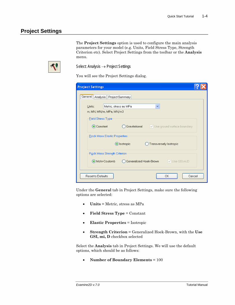
The Project Settings option is used to configure the main analysis parameters for your model (e.g. Units, Field Stress Type, Strength Criterion etc). Select Project Settings from the toolbar or the Analysis menu.

Select: Analysis → Project Settings

You will see the Project Settings dialog.

Under the General tab in Project Settings, make sure the following options are selected:

• Units = Metric, stress as MPa

• Field Stress Type = Constant

• Elastic Properties = Isotropic

• Strength Criterion = Generalized Hoek-Brown, with the Use GSI, mi, D checkbox selected

Select the Analysis tab in Project Settings. We will use the default options, which should be as follows:

• Number of Boundary Elements = 100



• Boundary Element Type = Constant

• Analysis Type = Plane Strain

• Matrix Solver Type = Jacobi Bi-Conjugate Gradient

Note: see the Examine2D Help topics for information about these options.

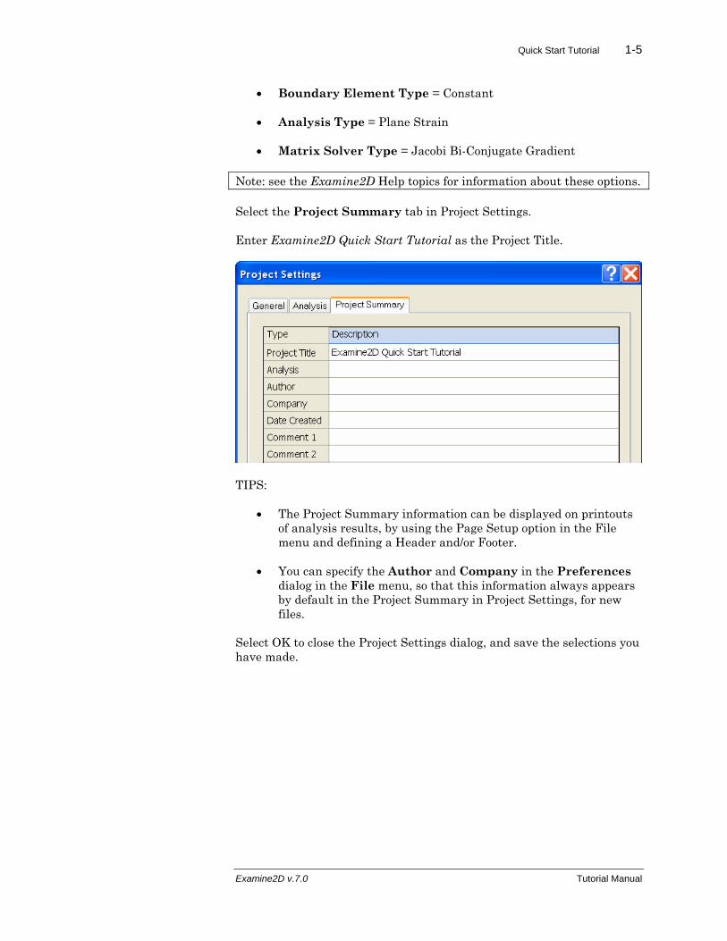
Select the Project Summary tab in Project Settings.

Enter Examine2D Quick Start Tutorial as the Project Title.

TIPS:

• The Project Summary information can be displayed on printouts of analysis results, by using the Page Setup option in the File menu and defining a Header and/or Footer.

• You can specify the Author and Company in the Preferences dialog in the File menu, so that this information always appears by default in the Project Summary in Project Settings, for new files.

Select OK to close the Project Settings dialog, and save the selections you have made.



Add Excavation Boundary

Now let’s add an Excavation Boundary. Select Add Excavation from the toolbar or the Boundaries menu.

Select: Boundaries → Add Excavation

Enter the following coordinates in the prompt line at the bottom right of the screen. Note: press Enter at the end of each line, to enter each coordinate pair, or single letter text command (e.g. “a” for arc or “c” for close).

Enter vertex [t=table,i=circle,esc=cancel]: 10 10 Enter vertex [...]: 16 10 Enter vertex [...]: 16 20 Enter vertex [...]: a

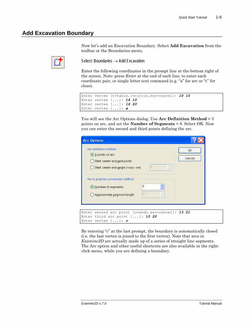
You will see the Arc Options dialog. Use Arc Definition Method = 3 points on arc, and set the Number of Segments = 8. Select OK. Now you can enter the second and third points defining the arc.

Enter second arc point [u=undo,esc=cancel]: 13 21 Enter third arc point [...]: 10 20 Enter vertex [...]: c

By entering “c” at the last prompt, the boundary is automatically closed (i.e. the last vertex is joined to the first vertex). Note that arcs in Examine2D are actually made up of a series of straight line segments. The Arc option and other useful shortcuts are also available in the right-click menu, while you are defining a boundary.



Stress Grid

By default, Examine2D automatically generates a Stress Grid, and computes the boundary element analysis, as soon as the first excavation is created.

The Stress Grid defines a grid of points at which stresses and other results are computed. The contours are generated within the Stress Grid from the results computed at the stress grid points. (The Stress Grid is the square bounding box which contains the contours).

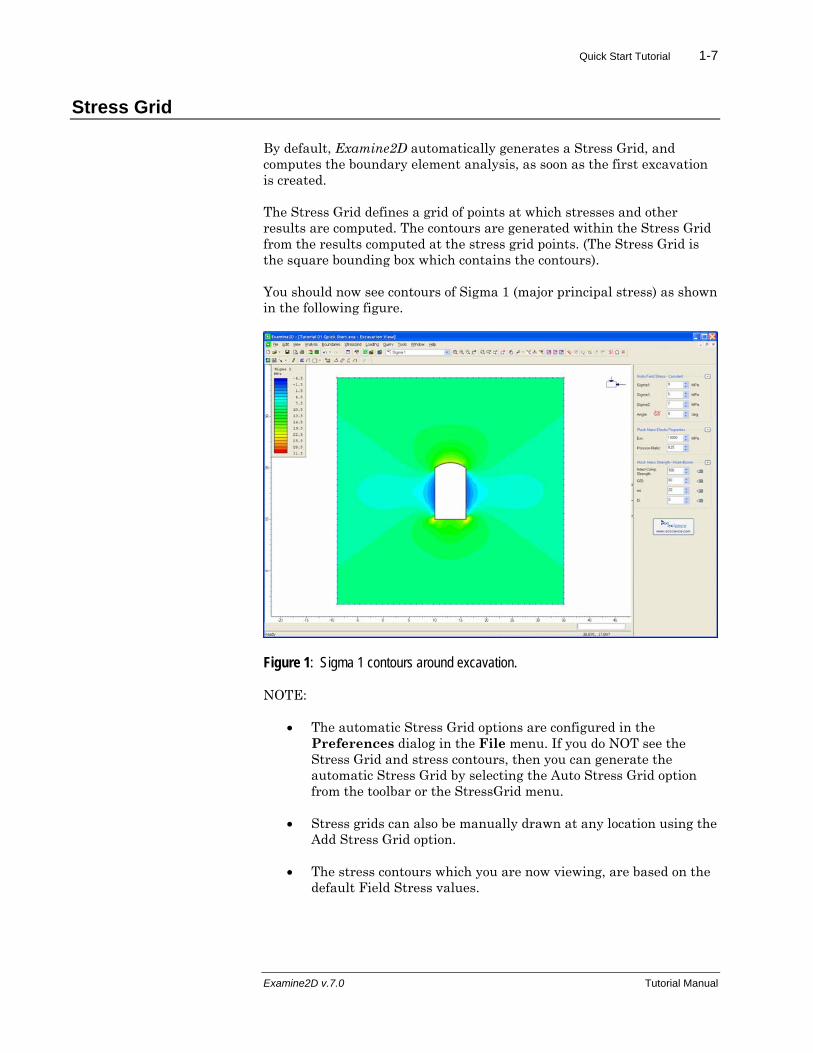
You should now see contours of Sigma 1 (major principal stress) as shown in the following figure.

Figure 1: Sigma 1 contours around excavation.

NOTE:

• The automatic Stress Grid options are configured in the Preferences dialog in the File menu. If you do NOT see the Stress Grid and stress contours, then you can generate the automatic Stress Grid by selecting the Auto Stress Grid option from the toolbar or the StressGrid menu.

• Stress grids can also be manually drawn at any location using the Add Stress Grid option.

• The stress contours which you are now viewing, are based on the default Field Stress values.



Copy Boundary

Now we will create a second Excavation boundary. The second boundary in this example will be identical to the first boundary, therefore, rather than entering coordinates again, we will simply use the Copy Boundary feature of Examine2D, to create a copy of the boundary.

We can use the following right-click shortcut for Copy Boundary:

1. Right click anywhere on the existing excavation boundary, and select Copy Boundary from the popup menu.

2. We will define the position of the new boundary, by defining a relative movement of 12 meters in the horizontal direction, and 0 meters in the vertical direction. A relative movement can be defined by typing the “@” character in the prompt line, followed by the relative x and y distance from the original object location.

3. Enter @12 0 in the prompt line:

Move from point [@=relative,esc=quit]: @12 0

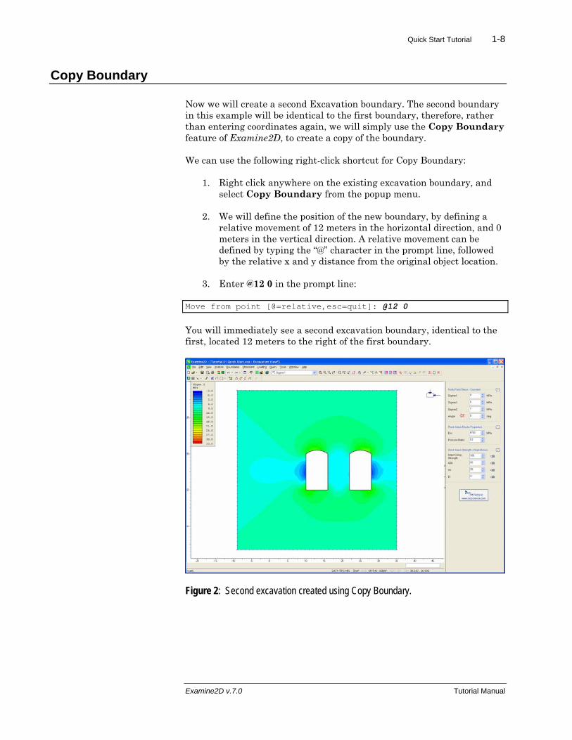
You will immediately see a second excavation boundary, identical to the first, located 12 meters to the right of the first boundary.

Figure 2: Second excavation created using Copy Boundary.



Auto Stress Grid

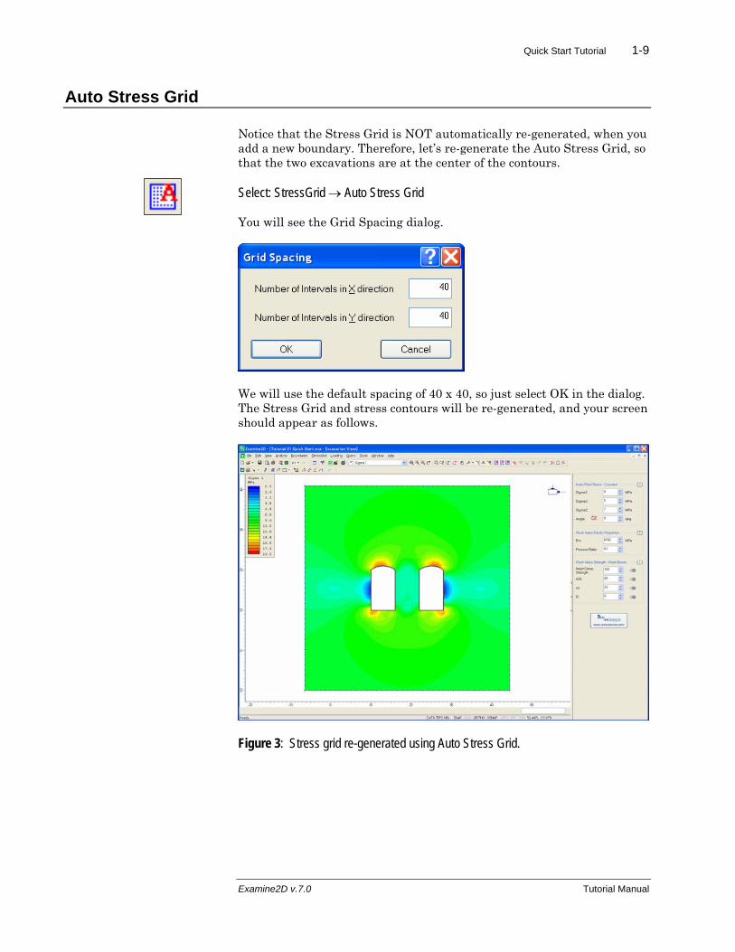
Notice that the Stress Grid is NOT automatically re-generated, when you add a new boundary. Therefore, let’s re-generate the Auto Stress Grid, so that the two excavations are at the center of the contours.

Select: StressGrid → Auto Stress Grid

You will see the Grid Spacing dialog.

We will use the default spacing of 40 x 40, so just select OK in the dialog. The Stress Grid and stress contours will be re-generated, and your screen should appear as follows.

Figure 3: Stress grid re-generated using Auto Stress Grid.



Field Stress

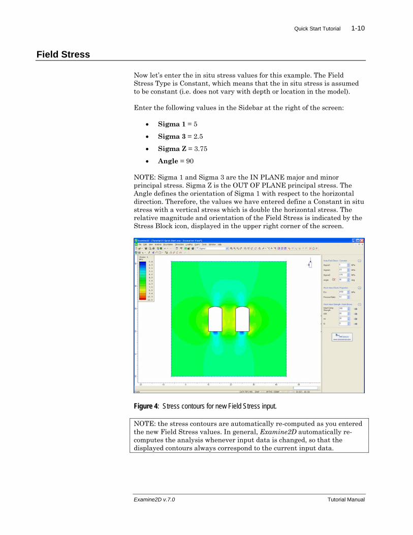
Now let’s enter the in situ stress values for this example. The Field Stress Type is Constant, which means that the in situ stress is assumed to be constant (i.e. does not vary with depth or location in the model).

Enter the following values in the Sidebar at the right of the screen:

• Sigma 1 = 5

• Sigma 3 = 2.5

• Sigma Z = 3.75

• Angle = 90

NOTE: Sigma 1 and Sigma 3 are the IN PLANE major and minor principal stress. Sigma Z is the OUT OF PLANE principal stress. The Angle defines the orientation of Sigma 1 with respect to the horizontal direction. Therefore, the values we have entered define a Constant in situ stress with a vertical stress which is double the horizontal stress. The relative magnitude and orientation of the Field Stress is indicated by the Stress Block icon, displayed in the upper right corner of the screen.

Figure 4: Stress contours for new Field Stress input.

NOTE: the stress contours are automatically re-computed as you entered the new Field Stress values. In general, Examine2D automatically re-computes the analysis whenever input data is changed, so that the displayed contours always correspond to the current input data.



Material Properties

Now let’s enter the elastic and strength properties for the rock mass. Enter the following Elastic parameters in the Sidebar.

• Em (rock mass Young’s modulus) = 10000

• Poisson’s Ratio = 0.2

Enter the following Strength parameters in the Sidebar.

• Intact Compressive Strength = 80

• GSI = 50

• mi = 17

• D = 0

Notice that the stress contours did NOT change (noticeably) when you entered the new elastic and strength parameters.

• The strength parameters have NO effect whatsoever on the calculated stresses or displacements in Examine2D. This is because the Examine2D analysis is elastic, and material failure cannot occur. The strength parameters are ONLY used to calculate the Strength Factor contours (i.e. degree of overstress, based on the elastic stress analysis).

• Young’s Modulus also has no effect on the elastic stress distribution (for an isotropic material).

• Poisson’s Ratio does affect the elastic stress distribution, however the effect is small for this example.

Estimating Input Parameters For the Generalized Hoek-Brown criterion (GSI, mi, D) option, if you select the “Pick” buttons beside the strength parameter edit boxes, this will take you to a chart or table, which allows you to estimate values for these parameters, according to rock type, rock structure etc.

This is left as an optional exercise to experiment with (if you make any changes in the dialogs, make sure the above strength parameters are entered in the Sidebar before proceeding with this tutorial).



Strength Factor

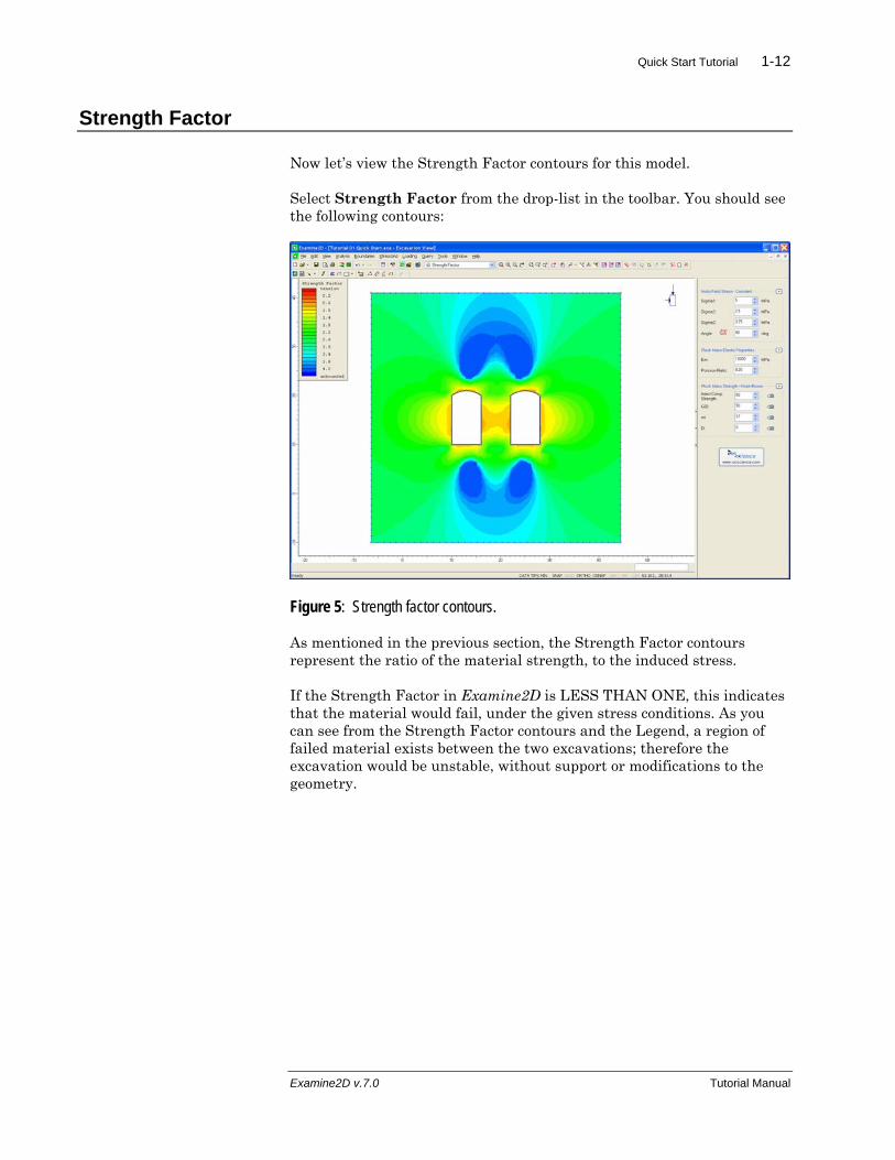
Now let’s view the Strength Factor contours for this model.

Select Strength Factor from the drop-list in the toolbar. You should see the following contours:

Figure 5: Strength factor contours.

As mentioned in the previous section, the Strength Factor contours represent the ratio of the material strength, to the induced stress.

If the Strength Factor in Examine2D is LESS THAN ONE, this indicates that the material would fail, under the given stress conditions. As you can see from the Strength Factor contours and the Legend, a region of failed material exists between the two excavations; therefore the excavation would be unstable, without support or modifications to the geometry.



Real Time Stress Analysis

Now we will demonstrate a unique feature of Examine2D – the ability to modify the excavation geometry, and view the updated stress analysis contours, in real time, as you edit the boundaries. Do the following:

1. Left click the mouse on either excavation (just a single click), so that the excavation boundary is highlighted by a dotted line.

2. Now if you hover the cursor over the excavation boundary, you will see the four-way arrow icon, which indicates that you can move the boundary with the mouse. Click and drag the excavation, and you will see that the analysis contours (in this case Strength Factor) are immediately updated, in real time, as you move the boundary. This capability is referred to as real time contouring or real time stress analysis in Examine2D.

Note: you cannot allow excavation boundaries to intersect or overlap. If you do this, you will see an error message when you release the mouse button.

Select Undo from the toolbar or the Edit menu, to undo the move and place the excavation back in its previous location.

Interactive Arrow Key Move A useful alternative method of moving the excavation boundaries, is by pressing the arrow keys, after selecting a boundary. This allows you to move the boundaries in controlled increments, in the horizontal or vertical directions. For example:

1. Left click the mouse on either excavation so that the excavation boundary is highlighted by a dotted line.

2. Now press the arrow keys (left, right, up or down), to move the excavation boundary. The contours are updated each time you press an arrow key.

3. Type the letter m followed by Enter in the prompt line. You will see the Move Increment dialog. This allows you to choose the move increment used each time you press an arrow key (the default is 1). Enter a value of 0.2 in the dialog and select OK.

4. Continue to press the arrow keys, and you will see that the excavation boundary now moves in smaller increments (0.2 meters) for each arrow key press. If you press and hold an arrow key, the excavation will move continuously, and the contours will be updated in real time.

Select Undo again, to undo the arrow key move, and place the excavation in its previous location.



Query

The Query capability of Examine2D allows you to obtain analysis results along any user-defined line or polyline (e.g. plot the stress along excavation boundaries).

There are two options for creating queries:

• Add Material Query – allows you to define a Query anywhere in the model.

• Query Boundary – allows you to automatically create a query exactly on a boundary.

Let’s first demonstrate Query Boundary. You can use the following right-click shortcut for Query Boundary:

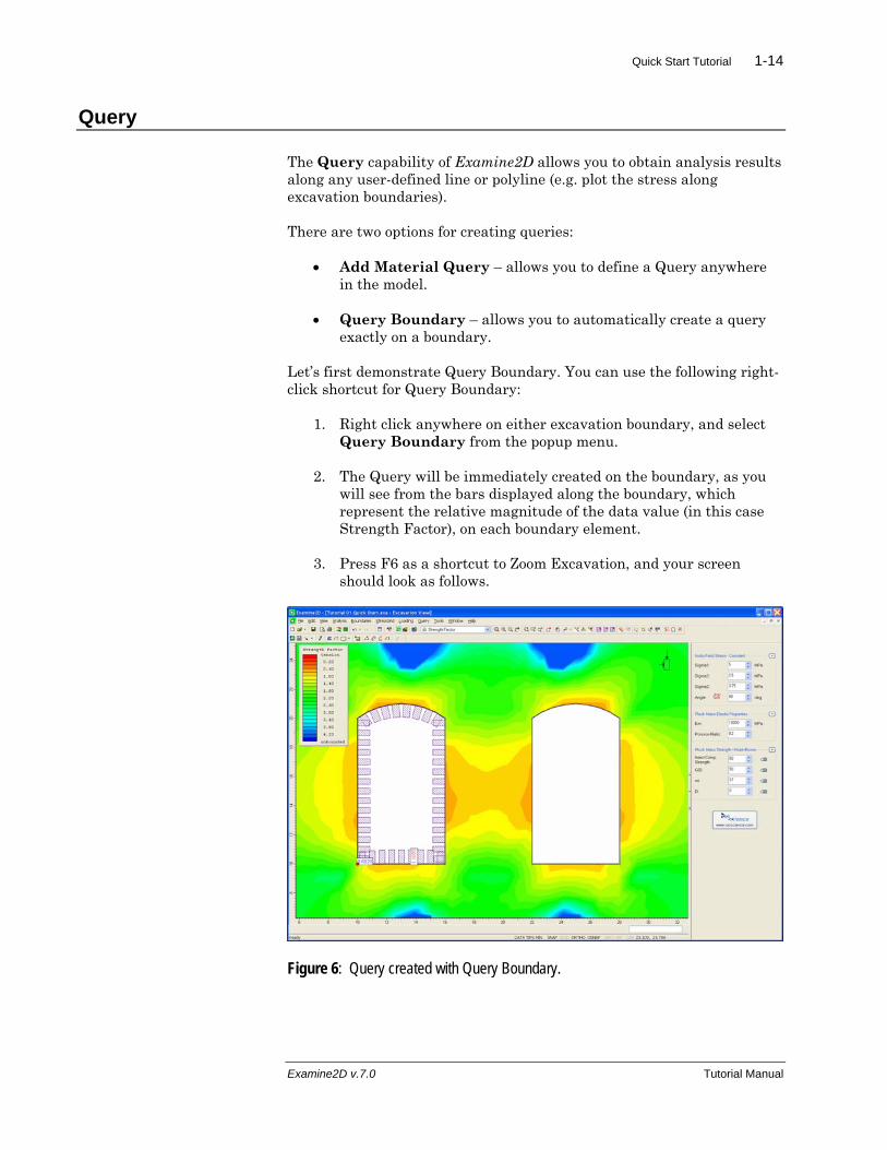
1. Right click anywhere on either excavation boundary, and select Query Boundary from the popup menu.

2. The Query will be immediately created on the boundary, as you will see from the bars displayed along the boundary, which represent the relative magnitude of the data value (in this case Strength Factor), on each boundary element.

3. Press F6 as a shortcut to Zoom Excavation, and your screen should look as follows.

Figure 6: Query created with Query Boundary.



The data which is generated by a Query can be:

• displayed directly on the model

• graphed

• exported to Excel or the clipboard

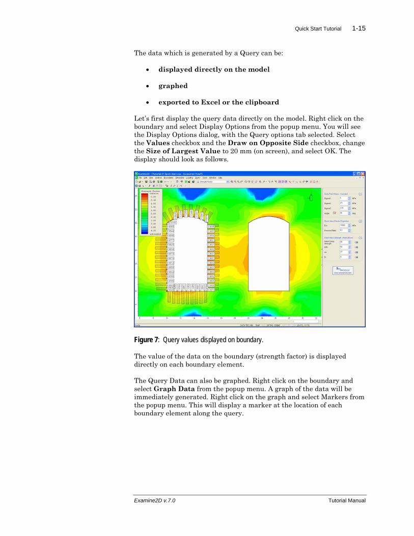
Let’s first display the query data directly on the model. Right click on the boundary and select Display Options from the popup menu. You will see the Display Options dialog, with the Query options tab selected. Select the Values checkbox and the Draw on Opposite Side checkbox, change the Size of Largest Value to 20 mm (on screen), and select OK. The display should look as follows.

Figure 7: Query values displayed on boundary.

The value of the data on the boundary (strength factor) is displayed directly on each boundary element.

The Query Data can also be graphed. Right click on the boundary and select Graph Data from the popup menu. A graph of the data will be immediately generated. Right click on the graph and select Markers from the popup menu. This will display a marker at the location of each boundary element along the query.



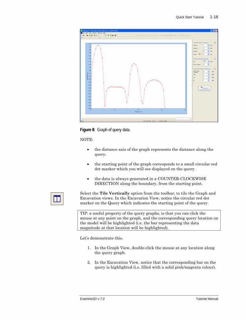
Figure 8: Graph of query data.

NOTE:

• the distance axis of the graph represents the distance along the query.

• the starting point of the graph corresponds to a small circular red dot marker which you will see displayed on the query.

• the data is always generated in a COUNTER-CLOCKWISE DIRECTION along the boundary, from the starting point.

Select the Tile Vertically option from the toolbar, to tile the Graph and Excavation views. In the Excavation View, notice the circular red dot marker on the Query which indicates the starting point of the query.

TIP: a useful property of the query graphs, is that you can click the mouse at any point on the graph, and the corresponding query location on the model will be highlighted (i.e. the bar representing the data magnitude at that location will be highlighted).

Let’s demonstrate this.

1. In the Graph View, double-click the mouse at any location along the query graph.

2. In the Excavation View, notice that the corresponding bar on the query is highlighted (i.e. filled with a solid pink/magenta colour).



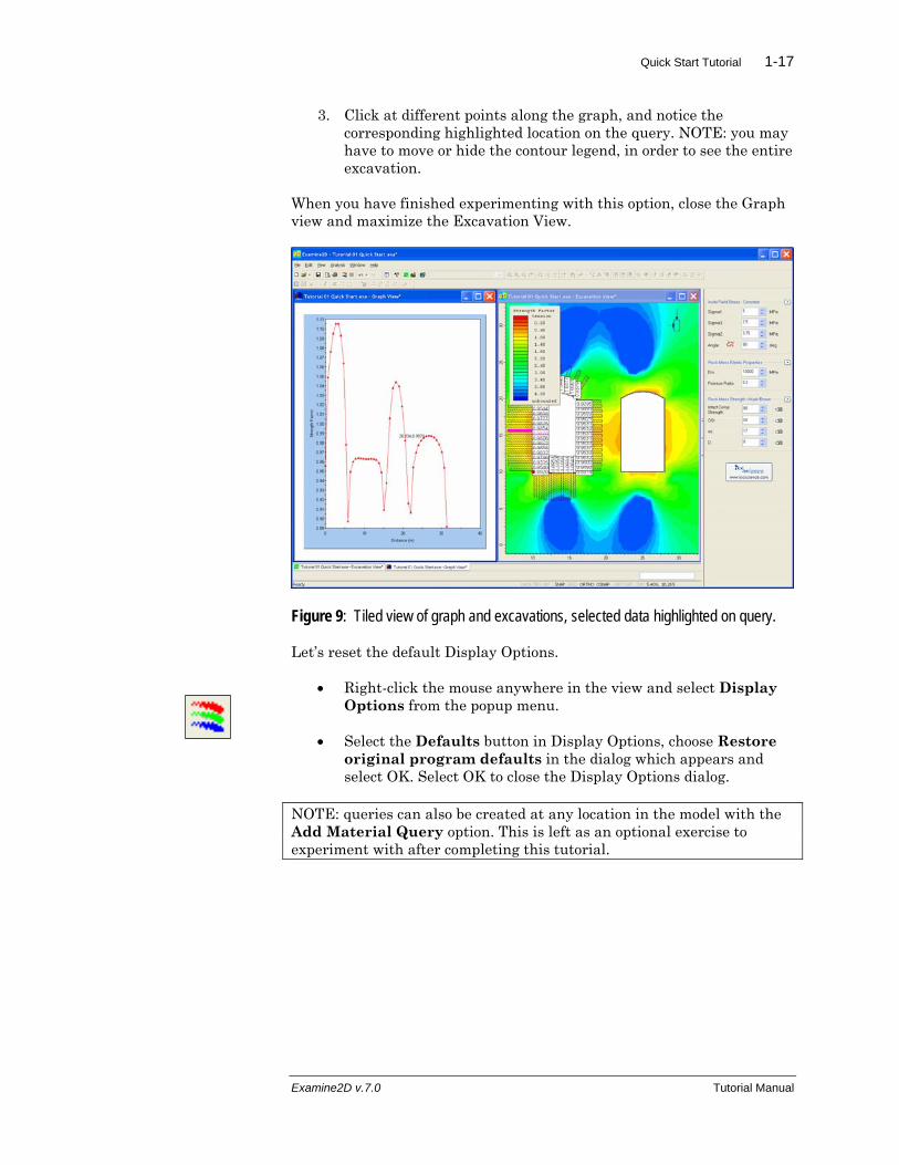
3. Click at different points along the graph, and notice the corresponding highlighted location on the query. NOTE: you may have to move or hide the contour legend, in order to see the entire excavation.

When you have finished experimenting with this option, close the Graph view and maximize the Excavation View.

Figure 9: Tiled view of graph and excavations, selected data highlighted on query.

Let’s reset the default Display Options.

• Right-click the mouse anywhere in the view and select Display Options from the popup menu.

• Select the Defaults button in Display Options, choose Restore original program defaults in the dialog which appears and select OK. Select OK to close the Display Options dialog.

NOTE: queries can also be created at any location in the model with the Add Material Query option. This is left as an optional exercise to experiment with after completing this tutorial.



Displacements

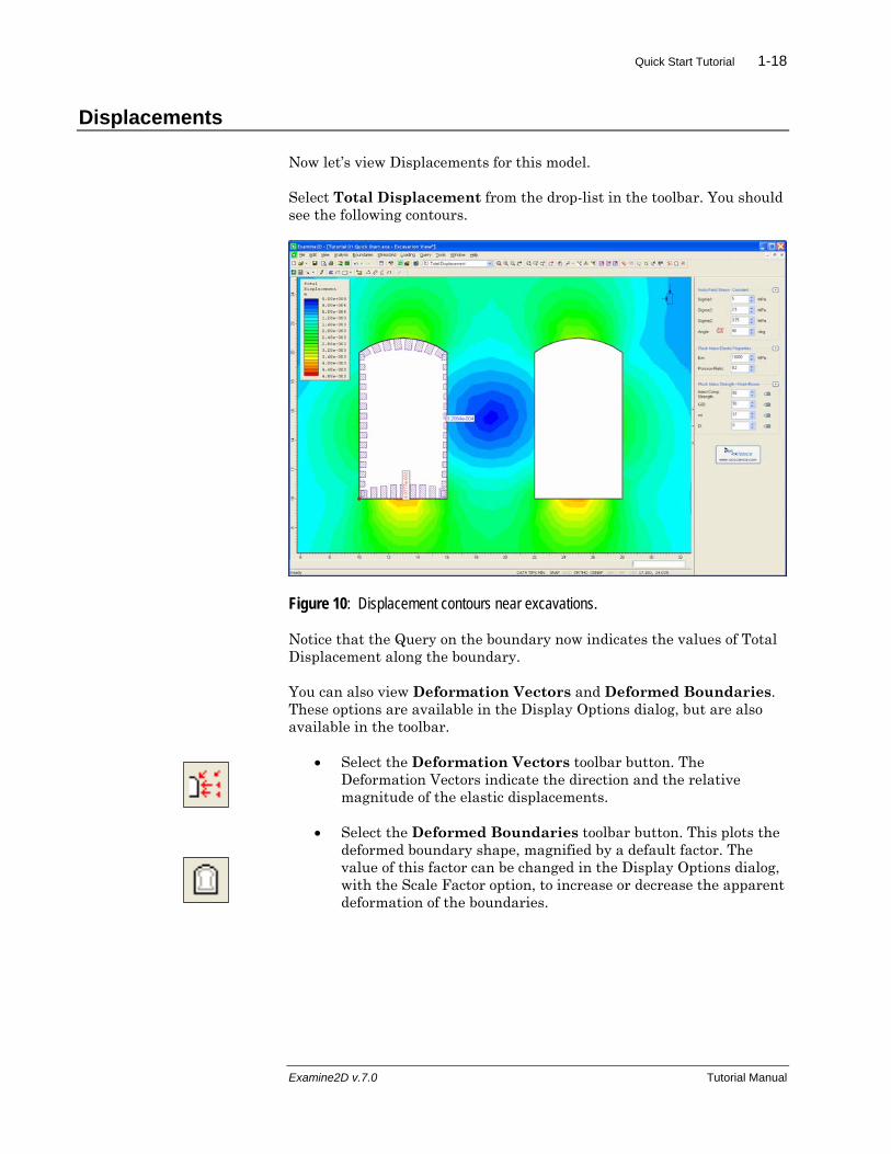
Now let’s view Displacements for this model.

Select Total Displacement from the drop-list in the toolbar. You should see the following contours.

Figure 10: Displacement contours near excavations.

Notice that the Query on the boundary now indicates the values of Total Displacement along the boundary.

You can also view Deformation Vectors and Deformed Boundaries. These options are available in the Display Options dialog, but are also available in the toolbar.

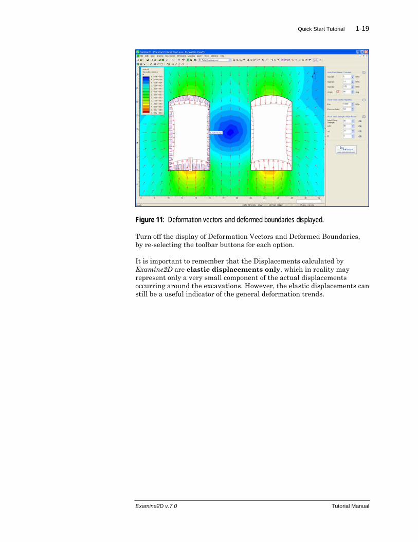
• Select the Deformation Vectors toolbar button. The Deformation Vectors indicate the direction and the relative magnitude of the elastic displacements.

• Select the Deformed Boundaries toolbar button. This plots the deformed boundary shape, magnified by a default factor. The value of this factor can be changed in the Display Options dialog, with the Scale Factor option, to increase or decrease the apparent deformation of the boundaries.



Figure 11: Deformation vectors and deformed boundaries displayed.

Turn off the display of Deformation Vectors and Deformed Boundaries, by re-selecting the toolbar buttons for each option.

It is important to remember that the Displacements calculated by Examine2D are elastic displacements only, which in reality may represent only a very small component of the actual displacements occurring around the excavations. However, the elastic displacements can still be a useful indicator of the general deformation trends.



Stress Trajectories

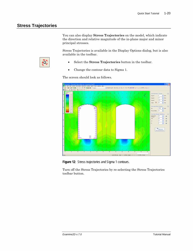
You can also display Stress Trajectories on the model, which indicate the direction and relative magnitude of the in-plane major and minor principal stresses.

Stress Trajectories is available in the Display Options dialog, but is also available in the toolbar.

• Select the Stress Trajectories button in the toolbar.

• Change the contour data to Sigma 1.

The screen should look as follows.

Figure 12: Stress trajectories and Sigma 1 contours.

Turn off the Stress Trajectories by re-selecting the Stress Trajectories toolbar button.



Failure Trajectories

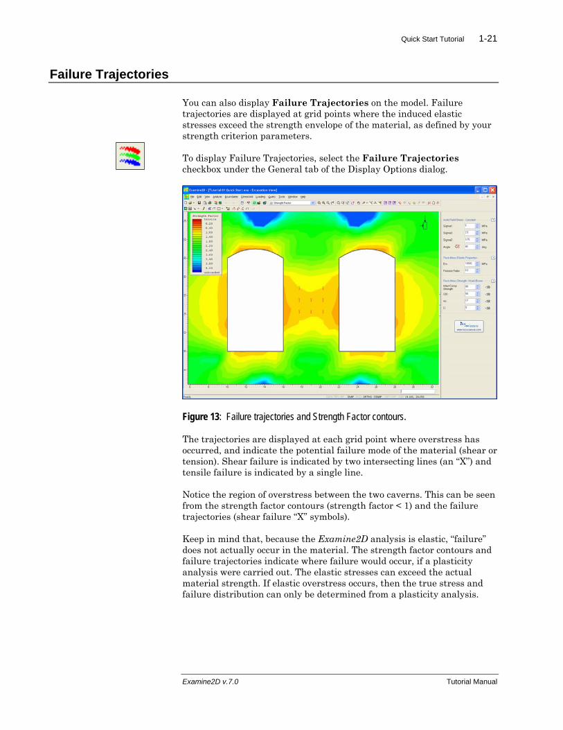
You can also display Failure Trajectories on the model. Failure trajectories are displayed at grid points where the induced elastic stresses exceed the strength envelope of the material, as defined by your strength criterion parameters.

To display Failure Trajectories, select the Failure Trajectories checkbox under the General tab of the Display Options dialog.

Figure 13: Failure trajectories and Strength Factor contours.

The trajectories are displayed at each grid point where overstress has occurred, and indicate the potential failure mode of the material (shear or tension). Shear failure is indicated by two intersecting lines (an “X”) and tensile failure is indicated by a single line.

Notice the region of overstress between the two caverns. This can be seen from the strength factor contours (strength factor < 1) and the failure trajectories (shear failure “X” symbols).

Keep in mind that, because the Examine2D analysis is elastic, “failure” does not actually occur in the material. The strength factor contours and failure trajectories indicate where failure would occur, if a plasticity analysis were carried out. The elastic stresses can exceed the actual material strength. If elastic overstress occurs, then the true stress and failure distribution can only be determined from a plasticity analysis.



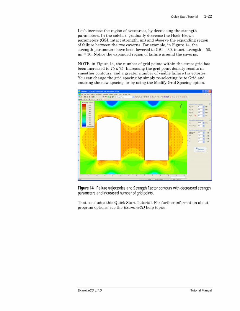
Let’s increase the region of overstress, by decreasing the strength parameters. In the sidebar, gradually decrease the Hoek-Brown parameters (GSI, intact strength, mi) and observe the expanding region of failure between the two caverns. For example, in Figure 14, the strength parameters have been lowered to GSI = 30, intact strength = 50, mi = 10. Notice the expanded region of failure around the caverns.

NOTE: in Figure 14, the number of grid points within the stress grid has been increased to 75 x 75. Increasing the grid point density results in smoother contours, and a greater number of visible failure trajectories. You can change the grid spacing by simply re-selecting Auto Grid and entering the new spacing, or by using the Modify Grid Spacing option.

Figure 14: Failure trajectories and Strength Factor contours with decreased strength parameters and increased number of grid points.

That concludes this Quick Start Tutorial. For further information about program options, see the Examine2D help topics.


tutorial examine 2d

Documents